Estimation of motion blur kernel parameters using regression convolutional neural networks

Abstract

Many deblurring and blur kernel estimation methods use MAP or classification deep learning techniques to sharpen an image and predict the blur kernel. We propose a regression approach using neural networks to predict the parameters of linear motion blur kernels. These kernels can be parameterized by its length of blur and the orientation of the blur.This paper will analyze the relationship between length and angle of linear motion blur. This analysis will help establish a foundation to using regression prediction in uniformed motion blur images.

1 Introduction

Linear motion blur has been studied as a model for camera shake, camera platform movement, and moving objects during imaging. This study was designed as a foundation to model atmospheric turbulence. The effects of atmospheric turbulence are generally modeled by a spatially-varying blurred image which can be modeled as a superposition of linear motion blurs [1, 2]. Linear motion blur kernels are parameterized by length and orientation. In this work, we study the ability to accurately estimate the length and angle parameters of a uniform linear motion blur. The results may then be used as a foundation upon which to build methods to estimate spatially-varying blur parameters and to serve as a baseline in subsequent studies.

A uniform blurred image can be described by

$$I_{b}=K*I_{s}+N,$$ (1)

where $I_{b}$ is the blurred image, $K$ is the blur kernel, $I_{s}$ is the sharp latent image, $N$ is additive noise, and $*$ is the convolution operator. Note that this formulation assumes a uniform blur since the same kernel $K$ is used across the entire image.

This paper presents an exploration in motion blur kernels including a scope outside of squared odd shaped kernels. The created dataset is used to train VGG16 [3] as a regression network to predict motion blur kernel parameters. The network is analyzed using the $R^{2}$ score which is a common regression analysis as well as a deconvolved error ratio (the error ratio between deconvolving using the predicted vs actual blur kernel).

The organization of this paper is as follows. In Section 2, we discuss previous work, including classical deblurring and deep learning deblurring methods. In Section 3, we describe in detail the exploration of the linear blur kernel parameter space as well as the creation of a blurred dataset for deep learning training. In Section 4, we discuss the process for regression blur parameter prediction and in Section 5, we present results of our regression prediction method and compare them to previous work. Finally, in Section 6, we conclude and briefly discuss our future work.

2 Related Work

Deblurring and kernel blur estimation has been extensively studied in computer vision, with applications of recovering the sharp image from blurry images caused by camera shake, fast moving objects in frame, or atmospheric turbulence. Prior to deep learning methods, many researchers used a maximum a posteriori (MAP) approach for both blur kernel estimation and deblurring. Two commonly used varieties of MAP are implicit regularization as seen in [4, 5] and explicit edge prediction based approaches like those in [6, 7, 8, 9, 10]. While many approaches have used MAP to estimate both the latent image and the blur kernel, Levin et al. [11, 12] prove that this approach tends to favor the no-blur explanation (i.e., that the kernel is an impulse and the “deblurred” image is the blurry image) instead of converging to the true blur kernel and latent sharp image. Moreover, it is advocated that estimating only the blur kernel is a better approach since there are fewer parameters to estimate than if one were to also estimate the latent sharp image. They use an Expectation-Maximization (EM) framework to optimize their kernel prediction while using either a Gaussian or sparse prior. More recently methods have considered using deep learning approaches to estimate the blur kernel [13], estimate the latent sharp image [14], or both [15].

Edge based approaches in a MAP framework use extracted edges as an image prior in the MAP optimization. Cho et al. [6] introduce a gradient computation using derivatives of the image to compute edges. Money & Kang [8] use shock filters for edge detection. Cho et al. [7] use the Radon transform for edge based analysis; image deblurring may be achieved through the use of a MAP algorithm or by computing the inverse Radon transform informed by the detected edges. Jia [9] uses object boundary transparency as an estimation of edge location. Fergus et al. [10] introduce natural image statistics defined by distributions of image gradients as a prior.

Implicit regularization MAP approaches use different regularization terms to enforce desired image priors. Xu et al. [4] incorporate a regularization term to approximate the $L_{0}$ cost which improves computational speeds over alternative implicit sparse regularizations. This framework alternates between estimating the latent sharp image and the blur kernel in each iteration. Krishnan et al. [5] use a ratio of $L_{1}/L_{2}$ norms as a regularization to estimate the kernel. This helps with the attenuation of high frequencies that blur introduces in an image.

Although many of the previous works discussed above can estimate generalized blur kernels, some work specializes in motion blur kernel prediction. Whyte et al. [16] propose a new method of estimating motion blur by parametrizing a geometric model in terms of rotational velocity of the camera during exposure time. They modify the Fergus et al. [10] algorithm to implement non-uniform deblurring. Hirsch et al. [17] combine projective motion path blur models with efficient filter flow [18] to estimate motion blur at a patch level and deblur by modifying the Krishnan & Fergus [19] algorithm.

Recent methods using deep learning have used various architectures including Convolutional Neural Networks (CNNs) [20, 21, 15, 13], Generative Adversarial Networks (GANs) [14], and Fully Convolutional Networks (FCNs) [22] to tackle the problem of blur kernel prediction and deblurring. Sun et al. [20] use a CNN to classify the best-fit motion blur kernel for each image patch. They use 73 different motion blur kernels and are able to expand up to 361 kernels by rotation of their input image. Gong et al. [22] use an FCN to predict a motion flow map where each pixel has its own motion blur parameters. Li et al. [15] uses a mixture of deep learning and MAP to deblur an image. They use a binary classification CNN which is trained to predict the probability of whether the input is blurry or sharp. The classifier is used as a regularization term of the latent image prior in their MAP framework. Yan & Shao [13] use a two step process to predict blur parameters. Their first step includes a deep neural network to classify the type of blur and their second step is a general regression neural network to predict the parameters of the blur predicted in step one. Gong et al. [22] use an FCN to predict a motion flow map of the blurred image and use non-blind deconvolution to recover the sharp image. While many of these approaches are able to handle spatially varying blur, we focus on a thorough exploration of motion kernel parameters in uniform blur; this will serve as a framework for spatially varying blur in future work.

In this work we focus on motion blur kernels and expand on the complexity of defining a motion blur kernel. We analyze which motion blur kernels exist within different kernel shape sizes rather than using $N\times N$ odd kernels as often implicitly assumed in the implementation, likely for ease of coding. By exploring all the motion blur kernel possibilities for a suite of length and angle combinations, we train a CNN which uses regression prediction instead of classification. We also expand the range of additive noise to analyze Gaussian noise up to a variance of 10%.

3 Blur Kernels and Blurred Dataset

A linear blur kernel can be parametrized by the length $r$ and orientation $\theta$ of a line. To formulate a discrete blur kernel for application to a digital image using Equation (1), we carefully define the difference between a continuous line and a discrete pixel line. We also explore angle and length combinations that exist within linear motion blur kernels. Finally, we discuss how we use the 2014 COCO dataset to create a new blurred dataset for deep learning training purposes.

3.1 Continuous and Pixel Lines

In this and following discussions, we use the terminology “line” to refer to a line segment. We use $r$ to denote a Euclidean distance (which could be defined for either a continuous or discrete line), $r_{\infty}$ to denote a Chebyshev distance for a discrete line, $\theta\in(-90,90]$ to denote the orientation (angle) of a continuous line in degrees, and $\phi\in(-90,90]$ to denote the orientation (angle) of a discrete pixel line in degrees. A blur kernel has dimensions $h\times w$ pixels. For a given length $r$, we denote the set of possible continuous line angles as $\Theta\in(-90,90]$ degrees and the set of possible discrete pixel line angles as $\Phi\subseteq\Theta$. A line in a 2-dimensional (2D) continuous domain $\mathbb{R}^{2}$ can be described as a 1-dimensional (1D) object with zero width and length $r$. The orientation of a line can be described by the angle with respect to the horizontal axis; $\theta=0$ thus corresponds to a horizontal line and $\theta=90$ to a vertical line. A pixel line in a 2D discrete domain $\mathbb{Z}^{2}$ is defined on a 2D discrete pixel grid which gives the line a non-zero width and length $r$. Figure 1 illustrates a continuous line with parameters $(r,\theta)=(3,90)$ and a pixel line with parameters $(r,\phi)=(3,90)$.

Figure 1: A continuous line (left) with parameters $(r,\theta)=(3,90^{\circ})$ and pixel line (right) with parameters $(r,\phi)=(3,90^{\circ})$. Note that the pixel line has a width of 1 due to its definition on a 2D discrete grid.

One limitation in defining pixel lines is the interrelation between length and angle of the line. In essence, a shorter pixel line will limit the number of unambiguous angles that a pixel line can have. Figure 2(a) illustrates how multiple continuous lines with angle $\theta\in[0,30]$ can be interpreted by the same horizontal pixel line of Chebyshev length $r_{\infty}=2$. Similarly if we move to a pixel line of Chebyshev length $r_{\infty}=2$ and angle $\phi=45$ (see Figure 2(c)) we can fit many intermediate lines with angles $\theta\in[30,60]$. The four pixel lines illustrated in Figure 2 show the only four pixel lines that can be described for a Chebyshev length $r_{\infty}=2$ pixel line. This means that for smaller length motion blurs, there will be gaps in the angles that can be represented. For example, a length $r_{\infty}=2$ pixel line can only have angles of $\phi\in\{-45,0,45,90\}$ as illustrated in Figure 2.

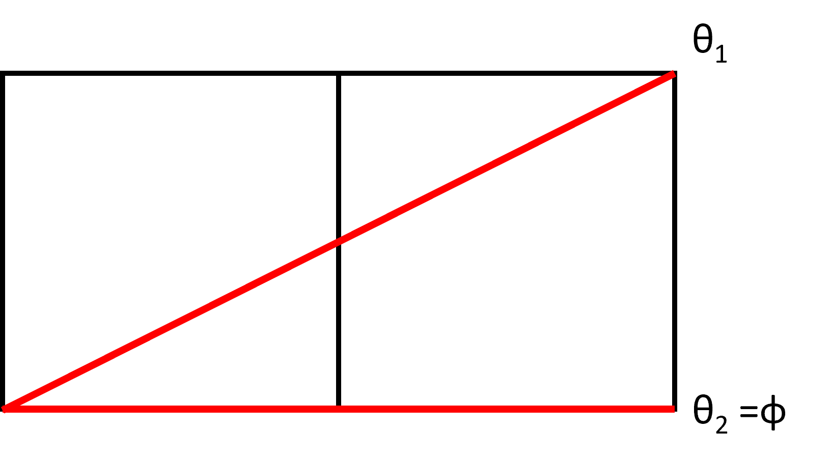
(a) Two distinct continuous lines in red (with $\theta_{1}=30^{\circ}$ and $\theta_{2}=\phi=0^{\circ}$) described by the same $\phi=0^{\circ}$ pixel line.

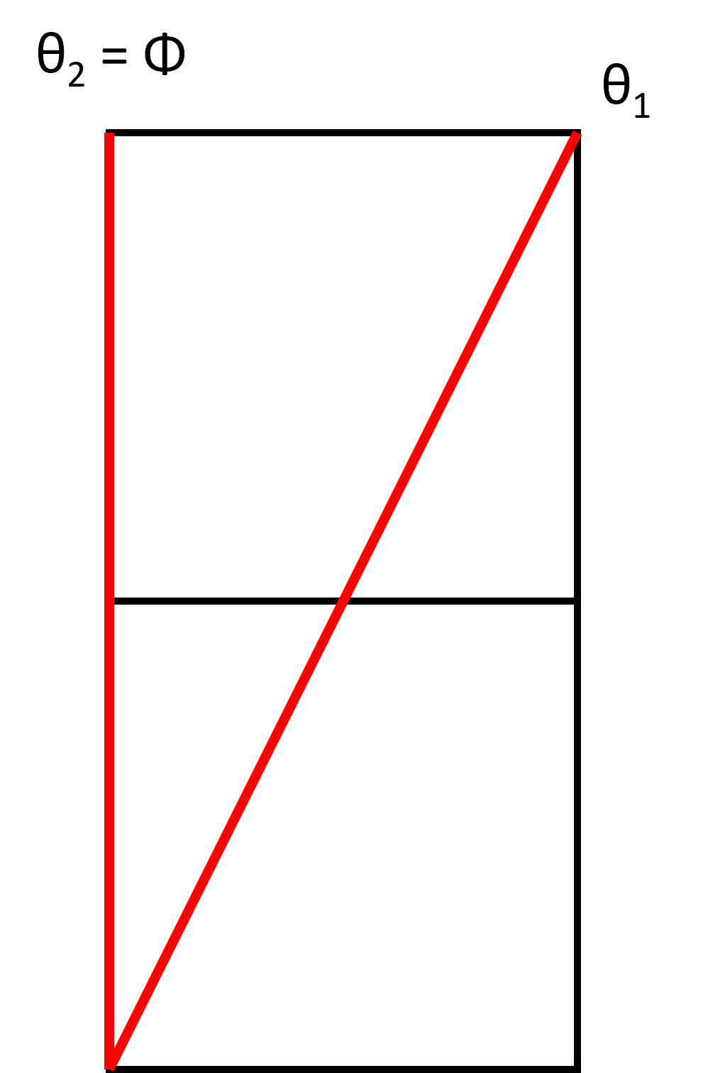
(b) Two distinct continuous lines in red (with $\theta_{1}=60^{\circ}$ and $\theta_{2}=\phi=90^{\circ}$) described by the same $\phi=90^{\circ}$ pixel line.

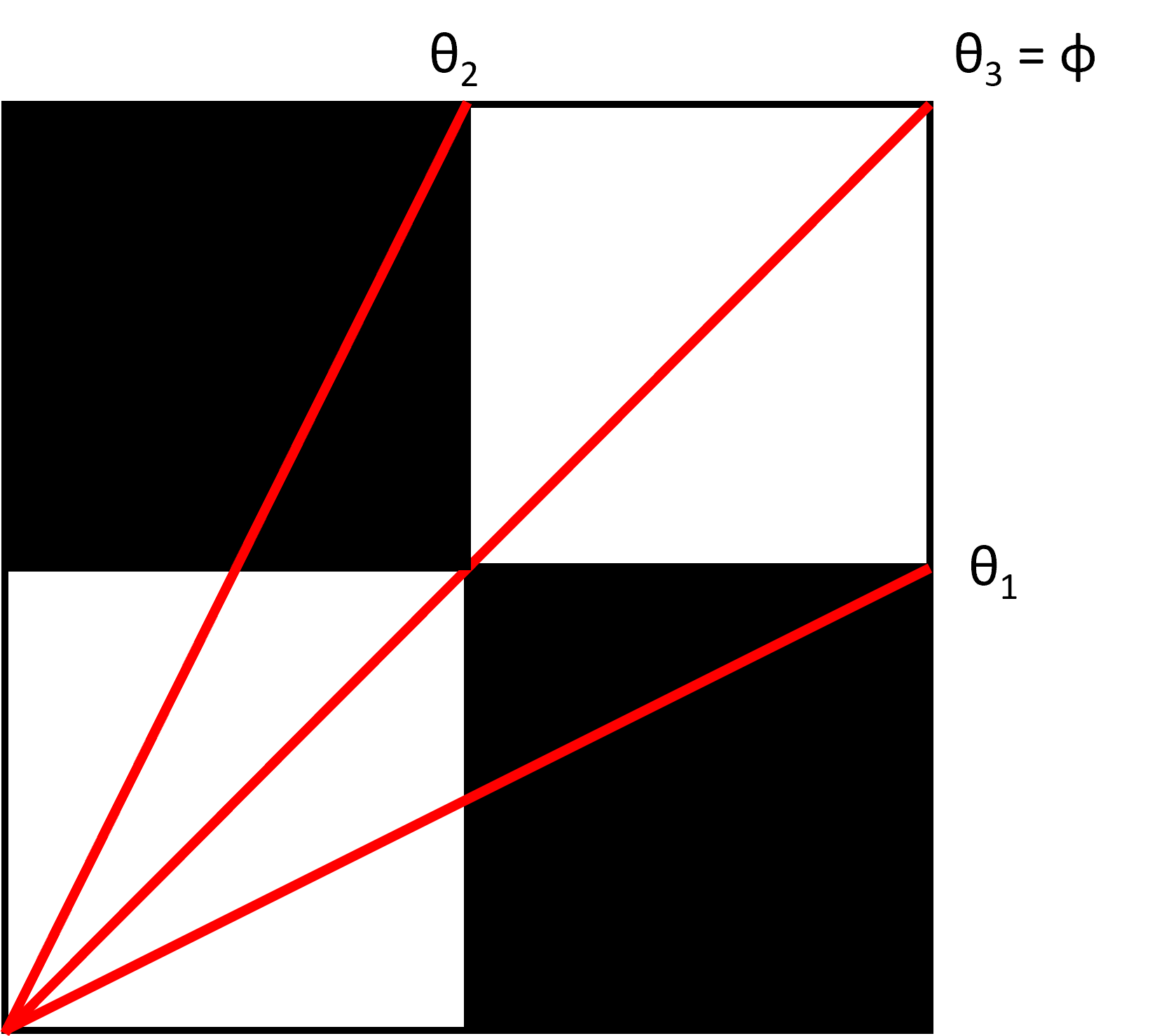
(c) Three distinct continuous lines in red (with $\theta_{1}=30^{\circ}$, $\theta_{3}=\phi=45^{\circ}$, and $\theta_{2}=60^{\circ}$ described by the same $\phi=45^{\circ}$ pixel line.

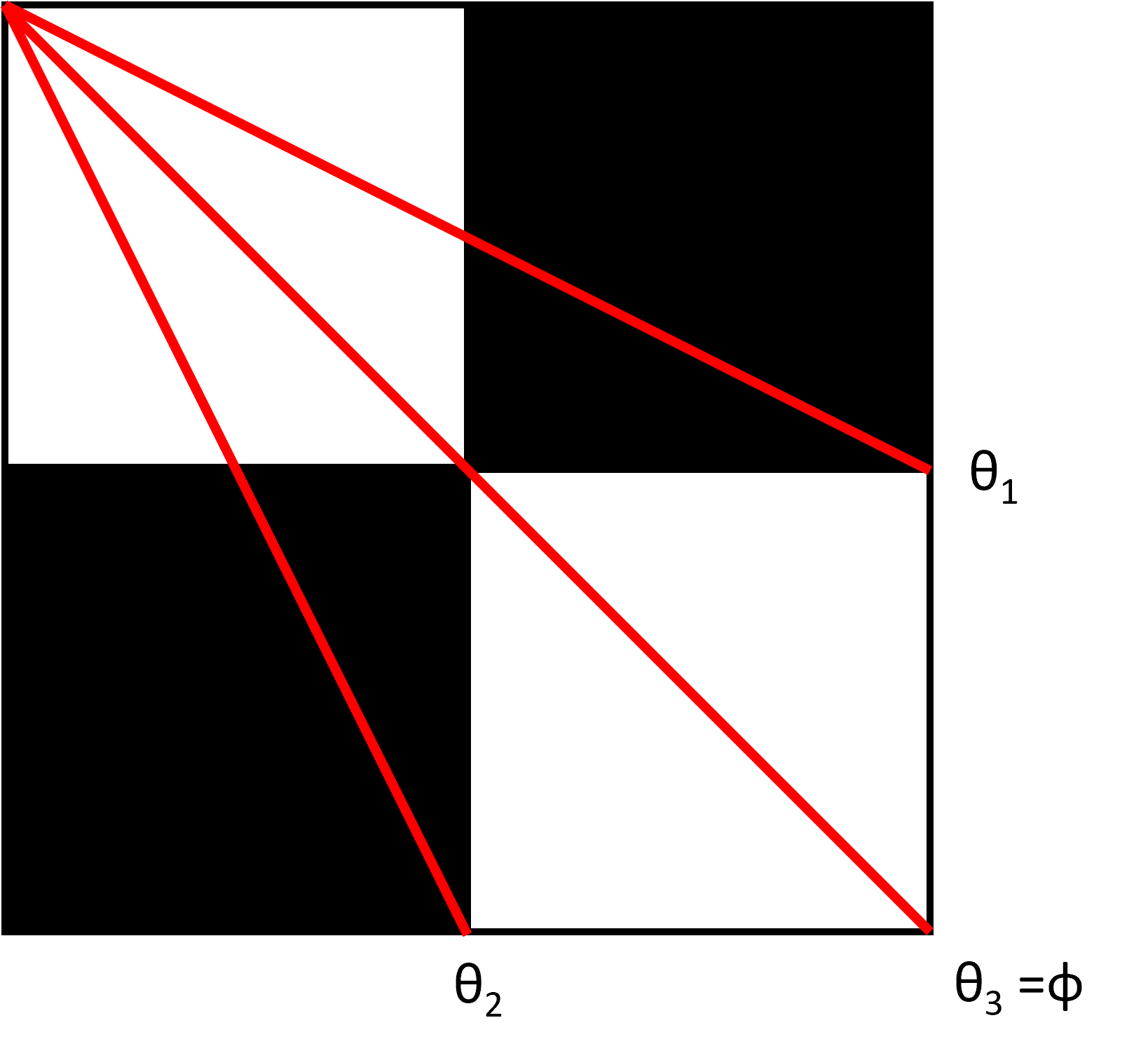
(d) Three distinct continuous lines in red (with $\theta_{1}=-30^{\circ}$, $\theta_{3}=\phi=-45^{\circ}$, and $\theta_{2}=-60^{\circ}$ described by the same $\phi=45^{\circ}$ pixel line.

Figure 2: Multiple continuous lines can be represented by the same pixel line of Chebyshev length $r_{\infty}=2$. Example continuous lines are shown in red, overlaid on the pixel line kernel that describes those continuous lines.

We also note that blur kernels may have two additional characteristics different from common conventions in image filter kernels: they may be non-square in dimension and they may be even in one or more dimensions. The $\phi=0$ and $\phi=90$ kernels in Figure 2 are $1\times 2$ and $2\times 1$ pixels, respectively; these two kernels are non-square and even in one dimension. The $\phi=\pm 45$ kernels in Figure 2 are both $2\times 2$ pixels; these two kernels are square but even in both dimensions. The assumption of square or odd-sized convolution kernels in the blur model described in Equation (1) is not mathematically necessary. The preference for square kernels is related to the symmetry of features both horizontally and vertically. The preference for odd-sized kernels is that there is an unambiguous center point to the kernel. This center point is commonly assumed to be associated with the pixel that is being processed.

3.2 Blur Kernel Creation

We explore the gaps in angles resulting from representation of continuous lines as pixel lines. We study a range of Euclidean lengths $r=2,3,\ldots,100$ and angles $\theta=-89,-88,\ldots,90$, and gather the resulting and unique $(r,\phi)$ discrete line parameter pairs.

We calculate the shape of an $h\times w$ kernel corresponding to an $(r,\theta)$ continuous line as follows:

$$h=\begin{cases}\lceil r\cos(\theta)\rceil,&\cos(\theta)\neq 0\\ 1,&\cos(\theta)=0\\ \end{cases}$$ (2)

$$w=\begin{cases}\lceil r\sin(\theta)\rceil,&\sin(\theta)\neq 0\\ 1,&\sin(\theta)=0,\\ \end{cases}$$ (3)

where $\lceil\cdot\rceil$ is the ceiling operator. The cases for $\cos(\theta)=0$ and $\sin(\theta)=0$ are to define a height or width of one for the horizontal and vertical cases, respectively. We use $r$ as the Euclidean distance labels which are drawn on top of the 2D discrete grid. The ceiling operator introduces a quantization error, since $r$ may result in a line ending mid-pixel. We include the pixel where $r$ ends as part of the motion blur kernel using the ceiling operator. The worst case for this quantization error is at angle of $\pm 45$ since the Euclidean length of a diagonal pixel is $\sqrt{2}$.

We use the line function from the skimage.draw library in python to draw a discrete line through the pixel grid. If $\phi$ is positive we draw a line from the lower-left corner $(h,0)$ to the upper-right corner $(0,w)$ and if $\phi$ is negative we draw a line from the upper-left corner $(0,0)$ to the lower-right corner $(h,w)$.

For each length $r=2,3,\ldots,100$, we generate a discrete blur kernel associated with a continuous line of length $r$ and angle $\theta=0,1,\ldots,90$. We then group all the angles $\theta\in\Theta$ that resulted in the same pixel line (e.g., see Figure 2). We must define a unique single discrete angle $\phi$ for each group of angles $\Theta$ for use as a training label:

$$\phi=\begin{cases}0,&0\in\Theta\\ 90,&90\in\Theta\\ \lceil\text{median}(\Theta)\rceil,&else\end{cases}.$$ (4)

Note that this definition of $\phi$ has two special cases. If the collection contains $\theta=0$, i.e., $0\in\Theta$, we know that the kernel is consistent with a horizontal line (see Figure 2(a)) and we assign $\phi=0$. Similarly, if the collection contains $\theta=90$, i.e., $90\in\Theta$, we know that the kernel is consistent with a vertical line (see Figure 2(b)) and we assign $\phi=90$. These special cases avoid the median operator assigning an erroneous label to a horizontal or vertical line.

We compute all possible $(r,\phi)$ combinations by generating the blur kernel for $r=2,3,\ldots,100$ and $\theta=0,1,\ldots 90$ and computing the resulting blur kernel angle $\phi$ using Equation (4). We span only positive angles $\theta\in[0,90]$ since we know that the negative kernels will be symmetric versions of the positive kernels (see also Figure 2(c) and (d)). The resulting combinations of $(r,\phi)$ parameters are the parameters of the unique discrete pixel lines. These parameter values are also what will be used as labels to train a network to predict the blur parameters from a blurry image (Section 4), using $(r,\phi)=(1,0)$ as labels for a non-blurred image.

(a) Unique combinations $(r,\phi)$ for discrete pixel lines.

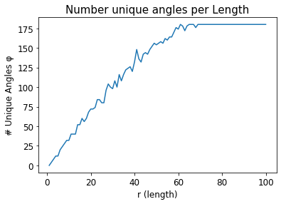
(b) Number of unique angles $\phi$ for each length $r$ in a discrete pixel line.

Figure 3: Length and angle pairs $(r,\phi)$ that are describable by a discrete pixel line. (a) Length $r$ and angle $\phi$ for all possible discrete blur kernels for $r\in[2,100]$ and $\phi\in(-90,90]$. (b) Number of angles that can be represented for a given length kernel. Note that shorter length kernels have many fewer possible angles that they can represent, including the four possible angles of $-45$, $0$, $45$, and $90$ for $r=2$.

Figure 3(a) illustrates the $(r,\phi)$ combinations as a scatter plot, where we note the existence of gaps where a continuous line cannot be described by a pixel line. As expected those gaps are larger for smaller lengths, indicating that there are limited unique pixel lines (blur kernels) for shorter blur lengths. Figure 3(b) plots the number of unique angles $\phi$ versus length $r$ where we note that we must have a line of approximately 70 pixels or larger in order to represent all orientations $\phi=-89,-88,\ldots,90$. We denote the unique combinations as $(r_{u},\phi_{u})$ and use these values to create a blurred dataset.

3.3 COCO Blurred Dataset

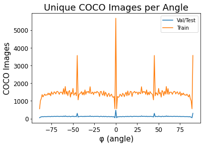
(a) Number of unique COCO images per angle in training and testing/validation datasets.

(b) Number of unique COCO images per length in training and testing/validation datasets.

Figure 4: Representation of COCO images versus length and angle.

We use the 2014 COCO dataset [23] to create a blurred dataset for training and validating a model for blind estimation of length and angle given only a blurry image. The 2014 COCO dataset consists of a training dataset with 82,783 images and a validation set of 40,504 images. We use the training dataset to create a blurred training dataset and we split (with no overlap) the validation dataset to create blurred validation and test datasets.

We create the blurred dataset by creating a blur generator that loops through the labeled pairs $(r_{u},\phi_{u})$, creating the corresponding blur kernel, and convolving the blur kernel with an image from the COCO dataset. We choose a random COCO image (without replacement) for each length $r_{u}$ to provide a variety of images in the blurred dataset. We encounter a dataset imbalance in lengths and/or angles represented in the blurred dataset due to the uneven representation of angles for shorter lengths (see Figure 3(b)). We improve the imbalance by creating a minimum of 175 blurred images per length. This implies that we end up using more unique COCO images for shorter blur lengths. Each run of the blur generator creates 21,789 blurred images. The creation of the training set used 12 parallel threads of the blur generator, each operating on a subset of the COCO dataset, creating a total of 261,468 blurred images. The validation and testing sets were each created with one run of the blur generator, creating a total of 21,789 blurred images for each. Figure 4 shows the number of unique COCO images versus length and angle for the training, validation, and testing datasets. We notice a spike in number of unique images for length $r=1$ and for angle $\phi=0$. This is due to the non-blurred images that are part of the dataset. We notice more unique images used for shorter lengths as the blur generator needs to loop through more images to complete the minimum threshold of images per length. We notice these small lengths create peaks in the angles of $\phi=[-45,0,45,90]$.

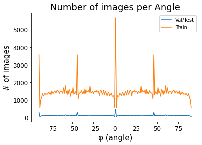
(a) Number of blurred images per angle.

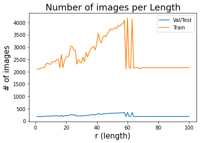
(b) Number of blurred images per length.

Figure 5: Distribution of blurred images for angle and length.

We note that there is an entanglement between angle and length, resulting in an inability to completely balance both length and angle in the blurred dataset. Figure 5 shows the distribution of labeled blurred images with respect to angle and length. Our choice to generate a minimum of 175 blurred images per length in the blur generator favors a more uniform length distribution [Figure 5(a)] This, however, results in peaks in the angle distribution [Figure 5(b)] due to the over-representation of certain angles for smaller lengths (see Figure 3). A choice to favor a more uniform angle distribution, however, would result in missing many shorter blur lengths, creating a more problematic data imbalance. While there are other choices that could be made regarding data imbalance here, we find that this blurred dataset can be used to train a network to accurately predict both length and angle.

4 Uniform Blur Prediction

We formulate blur length and angle estimation as a deep learning regression problem using the VGG16 [3] architecture as the backbone of our model. We trained VGG16 from scratch with TensorFlow’s default layer initializations to predict both the length and angle parameters for a linearly uniform motion blurred image. We modified the last layer of VGG16 to have two output nodes (corresponding to prediction of length and angle) with sigmoid activations. Since the sigmoid activation outputs values in the range $[0,1]$, we normalize length and angle to be in the range $[0,1]$ to train the model. The predicted length and angle parameters are re-scaled to their native ranges ($r\in[1,100]$, $\phi\in(-90,90]$) for validation.

Due to the fixed input size of VGG16 $(224\times 224)$, we created a TensorFlow data generator to randomly crop the blurred COCO images. We crop instead of resizing the image to maintain accuracy in the blur angle labels since a resize could change the aspect ratio of the image and thus the blur angle. If a blurred image was smaller than the input size for VGG16 then it was skipped and not used. In total there were 892 training, 5 validation, and 13 test images that were skipped. This results in less than $0.3\%$ of images skipped for each dataset.

We use the Adam optimizer to with a learning rate of 0.1 and epsilon of 0.1. We use the mean squared error (MSE) as the loss function. We empirically determined that a batch size of 50 minimized convergence issues. We train for 50 epochs, saving the weights for the best model throughout training and terminating training if the MSE performance has not improved within the previous 5 epochs. Training takes about 25 minutes per epoch and about 12 hours to fully train on an NVIDIA RTX-3090.

We performed multiple trainings of the network by adding different noise levels to each training. This resulted into four different models. The first model is trained with no noise and the other three models are trained with different levels of additive white Gaussian noise with variance $\sigma^{2}\in\{0.001,0.01,0.1\}$. We added the noise in our data generator after the image was cropped and normalized to the range $[0,1]$. In testing we test each model with the noiseless test set and by adding the three noise levels to the test set for an additional three test runs.

5 Experiments and Results

In this section, we present results using the $R^{2}$ metric for evaluating the regression model. We present results of the effects of additive noise on our model’s predictions. Finally we compare with other methods [5, 11] and evaluate using the error ratio score as introduced by [24].

5.1 Metrics

We validate the performance of blur estimation using metrics that measure the accuracy of the parameter estimation itself and also the quality of an image deblurred using the estimated kernel.

5.1.1 Accuracy of Parameter Estimation

In testing, we measure performance using the coefficient of determination, $R^{2}$. The coefficient of determination, $R^{2}$, measures the goodness of fit between actual known values of variable $y_{i}$ and estimated values $x_{i}$:

$$R^{2}=1-\frac{\sum_{i=1}^{n}(y_{i}-x_{i})^{2}}{\sum_{i=1}^{n}(y_{i}-\bar{y})^{2}},$$ (5)

where $\bar{y}$ is the mean of the known variables $y_{i}$ and $n$ is the number of samples [25]. The numerator $\sum_{i=1}^{n}(y_{i}-x_{i})^{2}$ is the sum of squares of the residual prediction errors and the denominator $\sum_{i=1}^{n}(y_{i}-\bar{y})^{2}$ is proportional to the variance of the known data. A perfect model will have zero residual errors and thus an $R^{2}=1$. A naïve model that always predicts the average of the data $\bar{y}$ will have equal numerator and denominator and thus an $R^{2}=0$. Models that have predictions worse than the naïve model will have $R^{2}<0$.

5.1.2 Quality of Deblurred Image

In addition to studying the accuracy of blur kernel estimation, we measure the quality of the image deblurred using the estimated blur kernel in a non-blind deblurring method (see Section 5.3). To measure the quality of the deblurred image, we use the error ratio as presented in [24]. The error ratio is motivated by the fact that, even with a perfectly estimated blur kernel, one may not be able to perfectly predict the latent sharp image. The error ratio $E_{\hat{k}}/E_{k}$ is computed by considering the error between the true sharp image and the latent sharp image recovered using the estimated blur kernel $E_{\hat{k}}$ and the error between the true sharp image and the latent sharp image recovered using the true blur kernel $E_{k}$. An error ratio of 1 indicates that the images deblurred using the estimated and true kernel are identical.

Any error metric can be used to define the error ratio, but we use the sum of squared differences (SSD) as in [24]. The error ratios are generally presented as a cumulative histogram for error ratios binned in the range $[1,4]$. As noted in [24], SSD error ratios above two tend to indicate significant perceptually noticeable distortion present in the image deconvolved with the estimated kernel.

5.2 Accuracy of Parameter Estimation

5.2.1 Noise-Free Predictions

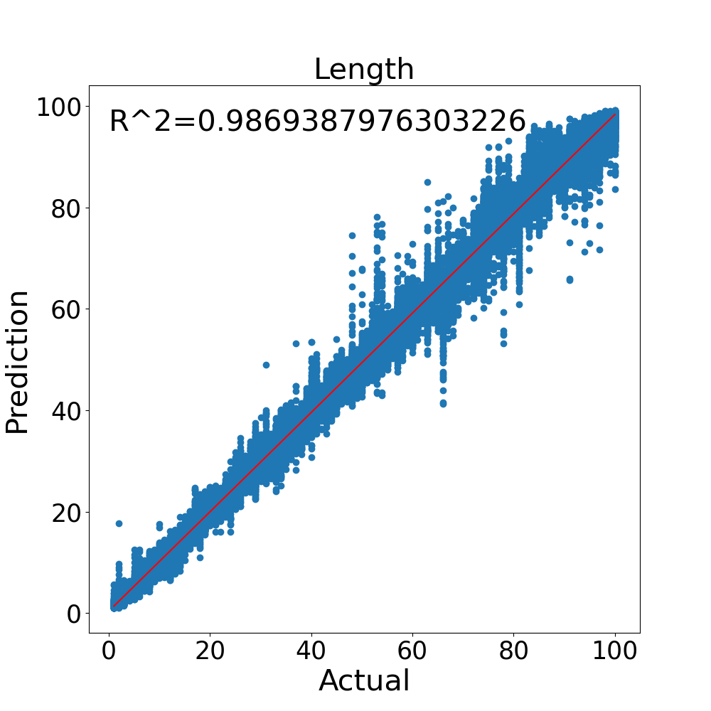
(a) Scatterplot of estimated versus actual length, $R^{2}=0.9869$.

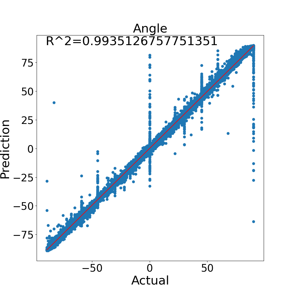
(b) Scatterplot of estimated versus actual angle, $R^{2}=0.9935$.

Figure 6: Scatterplots of estimated versus actual values for (a) length and (b) angle along with corresponding $R^{2}$ score. The individual estimates are represented as blue points and the best fit linear line is plotted in red.

A VGG-16 based model (see Section 4) was first trained on blurred images without any additive noise. Scatterplots of estimated versus actual length and angle are illustrated in Figure 6 along with the corresponding $R^{2}$ scores. We find the model to be highly accurate for prediction of both length and angle as demonstrated by the $R^{2}$ scores of 0.9869 and 0.9935, respectively. In Figure 6(a) we note a larger spread in estimated values as the length increases. This is not surprising, as larger blur lengths are expected to be more difficult to accurately estimate. In Figure 6(b) we note certain angles have a larger spread in estimated values. This is most notable for $\phi\in\{0,\pm 45,90\}$, but can be noted for other angles. This is due to errors in prediction for the smaller length kernels which have a limited set of angles. It is important to recall, however, that many of these incorrect angle predictions will result in a correct blur kernel. As an example, an image blurred with kernel parameters $(r,\phi)=(2,0)$ may have an angle prediction of $\hat{\phi}=27$. However, since blur kernels of length $r=2$ can only be represented by $\phi\in\{0,\pm 45,90\}$, the blur kernel created with parameters $(r,\phi)=(2,27)$ will generate the closest valid line of $(r_{u},\phi_{u})=(2,0)$.

5.2.2 Predictions with Additive Noise

Table 1: $R^{2}$ score for length prediction for training and testing under different levels of additive noise.

	Testing $\sigma^{2}$
Training $\sigma^{2}$	0	0.001	0.01	0.1
0	0.9869	-0.26	-3.17	-3.17
0.001	0.9607	0.9557	-1.14	-3.12
0.01	0.9527	0.9539	0.9523	-2.91
0.1	0.8923	0.8932	0.8960	0.8772

Table 2: $R^{2}$ score for angle prediction for training and testing under different levels of additive noise.

	Testing $\sigma^{2}$
Training $\sigma^{2}$	0	0.001	0.01	0.1
0	0.9935	0.8772	0.3935	0
0.001	0.9758	0.9754	0.6509	-0.16
0.01	0.9733	0.9735	0.9682	0.0128
0.1	0.8999	0.9009	0.9010	0.8834

We used the model from Section 5.2.1, trained on noise-free blurred images, and tested it on images with additive white Gaussian noise with variance $\sigma^{2}\in\{0.001,0.01,0.1\}$, corresponding to signal-to-noise (SNR) values of $\{30,20,10\}$ dB, respectively. Results for this experiment are shown in the first row of Table 1 and Table 2 for length and angle prediction, respectively. We note the estimation of the length parameter is more susceptible to noise than angle, resulting in a complete failure of prediction ($R^{2}$ scores less than 0) for even the smallest level of additive noise, $\sigma^{2}=0.001$. We hypothesize that additive noise can alter the intensity distribution along the blur path in a blurry image, creating the appearance of artificially shorter or longer blur paths. Those blur paths, however, will likely retain more characteristics of their angle for the same level of noise.

We trained three additional models using noisy blurred images with additive white Gaussian noise with variance $\sigma^{2}\in\{0.001,0.01,0.1\}$ and tested each of those models on noise-free and noisy images, i.e., for $\sigma^{2}\in\{0,0.001,0.01,0.1\}$. Results for those three models are in the second through fourth rows of Table 1 and Table 2 for length and angle prediction, respectively. We again note a higher sensitivity to noise in the prediction of length (Table 1) than angle (Table 2). We further note that the $R^{2}$ score decreases by $\sim 0.1$ for the model trained on the highest level of noise $\sigma^{2}=0.1$ compared to the noise-free model, but that the same model is robust to varying levels of noise. Finally we note that the models trained on noisy data appear to be robust to noise levels less than or equal to the noise level on which they are trained. This implies that a single model trained on a single noise level can yield accurate predictions even for smaller noise levels not seen in training.

In comparison to other methods that test under additive noise, most, e.g. [11, 7], test up to a Gaussian noise of $\sigma^{2}=0.01$ to simulate sensor noise. Krishnan et al. [5] tests noise of up to $\sigma^{2}=0.02$. Our model is tested up to $\sigma^{2}=0.1$ and demonstrates a higher tolerance for noise which can be an advantage when modeling atmospheric turbulence.

5.3 Quality of Deblurred Images

5.3.1 Deconvolution and Comparison Methods

We quantify the performance of our blur parameter estimation by using the expected path log likelihood (EPLL) method [26] to deconvolve the images using our predicted motion blur kernel and the ground truth blur kernel. We used the python implementation available at https://github.com/friedmanroy/torchEPLL. We replaced their Gaussian kernel with our linear motion blur kernel.

EPLL only accepts square, odd-sized blur kernels. This means we must zero pad our predicted parameter kernel to a square, odd-sized blur kernel. We zero padded the shortest side of the kernel on both sides to keep the kernel centered and padded to match the size of the longest side. If the longest side is even, however, this would result into an even-sized square kernel. We used a similar approach to [27] where we create four odd-sized kernels each zero padded with the line asymmetrically offset toward a different corner. We deconvolve the blurred image with each of the four kernels and average the four deconvolved images as the resulting deblurred image.

Additionally, we compare performance with other blur kernel estimation methods from Levin et al. [11] and Krishnan et al. [5]. Both Levin et al. [11] and Krishnan et al. [5] include methods for estimating the deblurred image. For fairness of comparisons, we use only the blur kernel estimate from both methods and use their blur kernel estimates in the same EPLL [26] deblurring framework as we use for our estimated blur kernels. For the method in [11], we used the Matlab implementation provided at https://webee.technion.ac.il/people/anat.levin/. We used the deconv_diage_filt_sps function and set a kernel prediction size of $(101,101)$. This is to allow prediction of the largest kernel size in our blurred dataset. It should be noted that the method in [11] estimates a blur kernel for each of the three channels in a color image; we applied EPLL to each channel using the kernel estimated for that channel. For the method in [5], we used the Matlab implementation provided at www.cs.nyu.edu/~dilip/wordpress/?page_id=159, again with kernel size of $(101,101)$.

5.3.2 Reduced Test Set

Due to the computational complexity of the EPLL deconvolution [26], as well as the deconvolution methods in Levin et al. [11] and Krishnan et al. [5], we generated reduced test datasets for these experiments. From our test dataset (see Section 3.3), we created two subsets to span length and angle. The first subset, subsequently referred to as Length 5 (L5), uses $5$ randomly selected blurred images for each length, totaling $500$ images. The second subset, subsequently referred to as Angle 3 (A3) uses $3$ randomly selected blurred images for each angle, totalling $540$ images. All images in these reduced test sets are noise free.

5.3.3 Error Ratio Comparisons

We calculated SSD error ratios for our proposed blur kernel estimation as well as those from Levin et al. [11] and Krishnan et al. [5] as seen in Figure 7. Recall that an error ratio of one indicates that deblurring with the estimated kernel results in an identical image to that deblurred with the ground truth kernel. An error ratio of two or higher is considered unacceptable as it was shown in [24] that such SSD error ratios indicate the presence of significant perceptually noticeable distortions in the latent image estimated using the estimated kernel. An error ratio less than 1 indicates that the image deblurred with the estimated kernel achieves a better match to the true sharp image than deblurring with the true kernel.

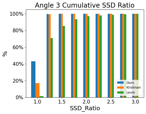
(a) SSD error ratio for the A3 dataset

(b) SSD error ratio for the L5 dataset

Figure 7: Error ratios for the A3 sub-dataset and L5 sub-dataset. Note that the bin at 1.0 includes error ratios $\leq 1.0$ and the bin at 3.0 includes error ratios $\geq 3.0$.

We note that we have the highest cumulative error ratio at one for both A3 and L5 datasets and that our method yields an error ratio of 1.25 or less for all images in the A3 and L5 test sets. This means that our model is able to predict more accurate kernels compared to the other methods. Since our method creates the kernel using linear parameters we are less prone to additive noise in the kernel. Levin et al.’s [11] kernel prediction has noise added in the kernel since many of the pixels that are supposed to be zero are instead small numbers close to zero. This noise can be seen to affect its results in kernel prediction. Krishnan et al. [19] thresholds the small elements of the kernel to zero which increases robustness to noise.

6 Conclusions

In this paper, we have studied in detail the limitation in representation of linear blur kernels, particularly for smaller length blurs. We noticed an entanglement between length and angle when it comes to representation of the two parameters, meaning that developing a dataset that is balanced in both length and angle is difficult. Much of the research done in linear blur has implicitly assumed square, odd-sized kernels. Exploring different sized kernels gives a complete implementation of possible linear motion blur kernels that can be discovered in natural blurred images.

The complete exploration of linear motion blur gives us an advantage of training a regressive deep learning model instead of a classification model as other deep learning methods implement. With regression we can estimate more accurate blur kernel parameters which are not limited by the model needing a prior predictive kernel size. Our robustness to noise has exceeded that of other methods, even testing to a higher level than most other methods. In particular, we see about a $10\%$ drop in the $R^{2}$ metric for a $10\%$ Gaussian noise. We note, however, that the model trained on 10% Gaussian noise was robust to noise levels less than 10%, indicating that single model can serve across a wide range of noise scenarios.

In future work, we will use this exploration of linear motion blur kernels as a baseline and foundation for spatially-varying blurs. We will expand this to a patch level to decompose a spatially-varying blur image into a superposition of locally uniform blur patches. This would give us a locally linear blur field to better model atmospheric turbulence in imagery.

Code, Data, and Materials Availability

The code necessary to implement the proposed method of kernel estimation as well as to generate the blurred dataset from the publicly available COCO dataset is available GitHub repository at https://github.com/DuckDuckPig/Regression_Blur.

References

- [1] B. R. Hunt, A. L. Iler, C. A. Bailey, and M. A. Rucci, “Synthesis of atmospheric turbulence point spread functions by sparse and redundant representations,” Optical Engineering, vol. 57, no. 2, p. 024101, 2018.
- [2] Y. Bahat, N. Efrat, and M. Irani, “Non-uniform blind deblurring by reblurring,” in 2017 IEEE International Conference on Computer Vision (ICCV), pp. 3306–3314, 2017.
- [3] K. Simonyan and A. Zisserman, “Very deep convolutional networks for large-scale image recognition,” arXiv preprint arXiv:1409.1556, 2014.
- [4] L. Xu, S. Zheng, and J. Jia, “Unnatural L0 sparse representation for natural image deblurring,” in Proceedings of the IEEE Conference on Computer Vision and Pattern Recognition (CVPR), June 2013.
- [5] D. Krishnan, T. Tay, and R. Fergus, “Blind deconvolution using a normalized sparsity measure,” in CVPR 2011, pp. 233–240, 2011.
- [6] S. Cho and S. Lee, “Fast motion deblurring,” in ACM SIGGRAPH Asia 2009 Papers, SIGGRAPH Asia ’09, (New York, NY, USA), Association for Computing Machinery, 2009.
- [7] T. S. Cho, S. Paris, B. K. P. Horn, and W. T. Freeman, “Blur kernel estimation using the radon transform,” in CVPR 2011, pp. 241–248, 2011.
- [8] J. H. Money and S. H. Kang, “Total variation minimizing blind deconvolution with shock filter reference,” Image and Vision Computing, vol. 26, no. 2, pp. 302–314, 2008.
- [9] J. Jia, “Single image motion deblurring using transparency,” in 2007 IEEE Conference on Computer Vision and Pattern Recognition, pp. 1–8, 2007.
- [10] R. Fergus, B. Singh, A. Hertzmann, S. T. Roweis, and W. T. Freeman, “Removing camera shake from a single photograph,” in ACM SIGGRAPH 2006 Papers, SIGGRAPH ’06, (New York, NY, USA), p. 787–794, Association for Computing Machinery, 2006.
- [11] A. Levin, Y. Weiss, F. Durand, and W. T. Freeman, “Efficient marginal likelihood optimization in blind deconvolution,” in CVPR 2011, pp. 2657–2664, 2011.
- [12] A. Levin, Y. Weiss, F. Durand, and W. T. Freeman, “Understanding and evaluating blind deconvolution algorithms,” in 2009 IEEE Conference on Computer Vision and Pattern Recognition, pp. 1964–1971, 2009.
- [13] R. Yan and L. Shao, “Blind image blur estimation via deep learning,” IEEE Transactions on Image Processing, vol. 25, no. 4, pp. 1910–1921, 2016.
- [14] Y. Zhang, Y. Xiang, and L. Bai, “Generative adversarial network for deblurring of remote sensing image,” in 2018 26th International Conference on Geoinformatics, pp. 1–4, 2018.
- [15] L. Li, J. Pan, W.-S. Lai, C. Gao, N. Sang, and M.-H. Yang, “Learning a discriminative prior for blind image deblurring,” in Proceedings of the IEEE Conference on Computer Vision and Pattern Recognition (CVPR), June 2018.
- [16] O. Whyte, J. Sivic, A. Zisserman, and J. Ponce, “Non-uniform deblurring for shaken images,” International journal of computer vision, vol. 98, pp. 168–186, 2012.
- [17] M. Hirsch, C. J. Schuler, S. Harmeling, and B. Schölkopf, “Fast removal of non-uniform camera shake,” in 2011 International Conference on Computer Vision, pp. 463–470, 2011.
- [18] M. Hirsch, S. Sra, B. Schölkopf, and S. Harmeling, “Efficient filter flow for space-variant multiframe blind deconvolution,” in 2010 IEEE Computer Society Conference on Computer Vision and Pattern Recognition, pp. 607–614, IEEE, 2010.
- [19] D. Krishnan and R. Fergus, “Fast image deconvolution using hyper-Laplacian priors,” Advances in neural information processing systems, vol. 22, 2009.
- [20] J. Sun, W. Cao, Z. Xu, and J. Ponce, “Learning a convolutional neural network for non-uniform motion blur removal,” in Proceedings of the IEEE Conference on Computer Vision and Pattern Recognition (CVPR), June 2015.
- [21] X. Xu, J. Pan, Y.-J. Zhang, and M.-H. Yang, “Motion blur kernel estimation via deep learning,” IEEE Transactions on Image Processing, vol. 27, no. 1, pp. 194–205, 2018.
- [22] D. Gong, J. Yang, L. Liu, Y. Zhang, I. Reid, C. Shen, A. van den Hengel, and Q. Shi, “From motion blur to motion flow: A deep learning solution for removing heterogeneous motion blur,” in Proceedings of the IEEE Conference on Computer Vision and Pattern Recognition (CVPR), July 2017.
- [23] T.-Y. Lin, M. Maire, S. Belongie, J. Hays, P. Perona, D. Ramanan, P. Dollár, and C. L. Zitnick, “Microsoft coco: Common objects in context,” in Computer Vision–ECCV 2014: 13th European Conference, Zurich, Switzerland, September 6-12, 2014, Proceedings, Part V 13, pp. 740–755, Springer, 2014.
- [24] A. Levin, Y. Weiss, F. Durand, and W. T. Freeman, “Understanding and evaluating blind deconvolution algorithms,” in 2009 IEEE conference on computer vision and pattern recognition, pp. 1964–1971, IEEE, 2009.
- [25] D. Chicco, M. J. Warrens, and G. Jurman, “The coefficient of determination R-squared is more informative than SMAPE, MAE, MAPE, MSE and RMSE in regression analysis evaluation,” PeerJ Computer Science, vol. 7, 2021.
- [26] D. Zoran and Y. Weiss, “From learning models of natural image patches to whole image restoration,” in 2011 international conference on computer vision, pp. 479–486, IEEE, 2011.
- [27] S. Wu, G. Wang, P. Tang, F. Chen, and L. Shi, “Convolution with even-sized kernels and symmetric padding,” in Advances in Neural Information Processing Systems (H. Wallach, H. Larochelle, A. Beygelzimer, F. d'Alché-Buc, E. Fox, and R. Garnett, eds.), vol. 32, Curran Associates, Inc., 2019.