Lessons from LHC on the LFV Higgs decays $h\to\ell_{a}\ell_{b}$ in the Two-Higgs Doublet Models

Abstract

The non-conservation of the lepton number has been explored at the LHC through the Lepton-Flavor Violating (LFV) Higgs decays $h\to\ell_{a}\ell_{b}$, with $\ell_{a,\,b}=e,\,\mu,\,\tau$ $(a\neq b)$. Current limits on these decays are a source of valuable information on the structure of the Yukawa and Higgs sectors. The LFV Higgs couplings can arise within the general Two-Higgs Doublet Model (2HDM); the predicted rates for these decay modes depend on the specific Yukawa structure being considered, ranging from a vanishing branching ratio at tree-level for some versions (2HDM-I, II, X, Y), up to large and detectable ratios within the general 2HDM-III. An attractive scenario is given by the texturized version of the model (2HDM-Tx), with the Yukawa matrices having some texture zeros, such as the minimal version with the so-called Cheng-Sher ansazt. We study the constraints on the parameter space of the 2HDM provided by experimental and theoretical restrictions, and use them to study the detection of LFV Higgs modes at LHC. We find several encouraging scenarios to the search for the decay $h\to\tau\mu$ that could be achieved in the High-Luminosity LHC. On the other hand, LFV Higgs couplings can also be induced at one-loop level in the 2HDM with neutrino masses, with the loops being mediated by neutrino interactions; we find that the resulting branching ratios are of order $10^{-7}$ at best, which is out of the reach of current and future phases of the LHC.

I Introduction

The Standard Model (SM), with a single Higgs doublet generating all the masses of the model, it has been confirmed at the Large Hadron Collider (LHC) thanks to the detection of a light Higgs boson with $m_{h}=125$ GeV Chatrchyan et al. (2012); Aad et al. (2012). The LHC program includes measuring the Higgs properties, to determine whether they are consistent with the SM predictions, or show some deviations that could point into the direction of physics beyond the SM Aad et al. (2016). So far, the LHC has been able to measure the Higgs couplings with $WW,\,ZZ$, and $b\bar{b},\tau^{+}\tau^{-},\mu^{+}\mu^{-}$, and indirectly the coupling with top quarks (from the Higgs coupling with photon and gluon pairs, which arise at one-loop).

On the other hand, the open problems of the SM, together with the results in areas such as neutrino physics and dark matter, suggest that some form of new physics should exist, to account for such phenomena. So far, a variety of experimental searches, including the energy, precision and cosmological frontiers, have imposed strong limits on the scale of new physics above $\mathcal{O}$(1) TeV Murayama (2007).

Models of new physics often include a Higgs sector with an extended spectrum and some new features Branco et al. (2012). Bounds on the flavor conserving Higgs couplings that arise in these models have been derived at LHC too Arroyo-Ure$\tilde{n}$a and Diaz-Cruz (2020). Moreover, some of these extensions of the SM, include a more flavored Higgs sector Diaz-Cruz (2003), which produces distinctive signals, such as the Flavor-Violating (FV) Higgs-fermions interactions; and in some cases the rates could be so large, that some suppression mechanism is required in order to build viable models Lorenzo Díaz-Cruz (2019).

In multi-Higgs doublet models, the Glashow-Weiberg theorem Glashow and Weinberg (1977) states that in order to avoid the presence of FV couplings in the Higgs-Yukawa sector, each fermion type (up- and down-type quarks) must acquire their masses from a unique Higgs doublet. Later on, it was found that it is possible to build realistic models with FV Higgs couplings, provided that the Yukawa matrices have a restricted form, i.e. with texture zeroes Cheng and Sher (1987). The extension of these ideas to the lepton sector was presented in Refs. Sher and Yuan (1992); Diaz-Cruz and Toscano (2000).

It is possible to probe these LFV effects at low-energies, through the LFV decays $\ell_{i}\to\ell_{j}\gamma$, $\ell_{i}\to\ell_{j}\ell_{j}\ell_{k}$. Furthermore, Ref. Diaz-Cruz and Toscano (2000) also proved that it is possible to have large rates for the LFV Higgs decays and to satisfy those low-energy LFV bounds. More realistic textures were considered in Diaz-Cruz et al. (2004), while the possibility to search for these LFV Higgs decays at hadron colliders was studied in Ref. Han and Marfatia (2001). The most recent search for LFV Higgs Decays at LHC, with center-of-mass energy $\sqrt{s}=13$ TeV and an integrated luminosity of $138$ fb^-1, has provided stronger bounds, in particular ATLAS reports both $\mathcal{BR}(h\to e\tau)<0.20\%$ and $\mathcal{BR}(h\to\tau\mu)<0.18\%$ ATL (2023), while the CMS collaboration concludes that $\mathcal{BR}(h\to e\tau)<0.22\%$ and ${\cal{B}}(h\to\tau\mu)<0.15\%$ for $137$ fb^-1 of accumulated data  Sirunyan et al. (2021), which are consistent with a zero value. The fact that the LHC has searched for these LFV Higgs boson decays modes, and has already presented strong bounds on the corresponding branching ratios, has motivated great interest from the theoretical side. Other models where the LFV Higgs signal is present are models with new physics, including: 2HDM Tsumura (2005); Kanemura et al. (2006); Primulando et al. (2020); Vicente (2019), models with a low-scale flavon mixing with the SM-like Higgs boson Arroyo-Ure$\tilde{n}$a et al. (2018), models with 3-3-1 gauge symmetry Hue et al. (2016); See-Saw model and its inverse version Pilaftsis (1992); Körner et al. (1993); Arganda et al. (2005); Thao et al. (2017), low scale see-saw Arganda et al. (2015); Hernández-Tomé et al. (2020), as well as SUSY models, including models with neutrino masses, such as see-saw MSSM Diaz-Cruz et al. (2009a) and the minimal SUSY SM (MSSM) Brignole and Rossi (2003); Diaz-Cruz et al. (2009b) at loop-level. Several type of methods has been used to calculate the LFV Higgs decays, for example the Mass Insertion Approximation (MIA) Arganda et al. (2016, 2017); Marcano and Morales (2020) or Effective Field approach Coy and Frigerio (2019), and the minimal SUSY SM (MSSM) Diaz-Cruz (2003). At the coming phase (with higher luminosity) it will be possible to derive more restrictive bounds, and one can analyze the consequences for the model building side.

In this paper we present a general discussion of the implications of the LFV Higgs decays searches at LHC, within the general 2HDM of type III Lorenzo Díaz-Cruz (2019). We start by study in the limits on $\mathcal{BR}(h\to\tau\mu)$ that can be achieved at LHC, as a function of the integrated luminosities that is projected for the future phases of the LHC. Then, we shall derive constraints on the model parameters, and discuss the lessons that LHC can impose on the model structure, and see how the resulting rate fit into the picture. We also discuss the expected rates for the LFV decay $h\to\ell_{a}\ell_{b}$, within the $\nu$2HDM, where such coupling is induced at one-loop level.

The organization of our paper goes as follows. Section II contains our parametrization for the Higgs couplings for the general 2HDM-III. Section III contains the study of the 2HDM-III parameter space which was obtained from low-energies processes and Higgs boson data. Results for the search for LFV Higgs decays at LHC and their future stages, namely, HL-LHC, HE-LHC and FCC-hh, are also presented in Sec. III. Section IV is dedicated to the one-loop calculation for the decay $h\to\ell_{a}\ell_{b}$ within the 2HDM of type I,II, including massive neutrinos, which are generated using the see-saw mechanism of type I. Finally, conclusions and perspectives are presented in Section V.

II The LFV Higgs couplings in the 2HDMs

The general two-Higgs doublet model admits the possibility to have LFV Higgs couplings, which have been explored already at LHC through the search for the decays $h\to\ell_{a}\ell_{b}$. The predicted rates for these decays depend on the specific model realization, ranging from a vanishing branching ratio at tree-level for 2HDM-I,II,X,Y, as well as the MFV implementation, up to large and detectable ratios within the version 2HDM-III, which depend on the specific Yukawa structure being considered. For instance the texturized version of the model (2HDM-Tx) with Yukawa matrices having for texture zeros Cheng and Sher (1987); Zhou (2004); Diaz-Cruz et al. (2004, 2005) , which has been found to reproduce the Cheng-Sher anzast Arroyo-Ureña et al. (2016); Carcamo Hernandez et al. (2007), provides the largest possible rates and it is strong by constrained at LHC (Run2), as we shall argue here. Next in importance could be the 2HDM where the LFV Higgs couplings are absent at tree level, that could be induced at one-loop, as it is the case for the $\nu$2HDM, which is the version of the 2HDM I,II but includes neutrino masses.

Thus, we start by presenting the coupling of the Higgs boson ($h$) with wector bosons ($W^{\pm},\,Z$). In this case we can write the interaction Lagrangian with terms of dimension-4, consistent with Lorentz symmetry and derivable from a renormalizable model, as follows:

$${\cal{L}}_{V}=\kappa_{W}gm_{W}hW^{+\mu}W^{-}_{\mu}+\kappa_{Z}\dfrac{gm_{Z}}{2c_{W}}hZ^{\mu}Z_{\mu}.$$ (1)

When the Higgs particle corresponds to the minimal SM, one has $\kappa_{W}=\kappa_{Z}=\kappa_{V}=1$, while values $\kappa_{W}=\kappa_{Z}\neq 1$ arise in models with several Higgs doubles, which respect the so-called custodial symmetry. In particular for models that include $N$ Higgs doublets $\Phi_{a}$, each one having a vacuum expectation value (vev) $v_{a}$, one has:

$$\kappa_{V}=\sum_{a}\dfrac{v_{a}}{v}O_{1a},$$ (2)

where $O_{1a}$ denotes the element of the matrix that diagonalizes the $\mathcal{CP}$-even Higgs mass matrix, with $h_{1}=h$ denoting the light SM-like Higgs boson; and $v^{2}=\sum_{a=1}^{N}v_{a}^{2}=246^{2}$ GeV².

On the other hand, the interaction of the Higgs with fermion $f$, with $f=q$ or $\ell$ for quarks and leptons, respectively, can also be written in terms of a dimension-4 Lagrangian that respects Lorentz invariance, namely:

$${\cal{L}}_{f}=h\bar{f}_{i}(S_{ij}+i\gamma_{5}P_{ij})f_{j}.$$ (3)

The $\mathcal{CP}$-conserving ($\mathcal{CP}$C) and $\mathcal{CP}$-violating ($\mathcal{CP}$V) factors $S_{ij}$ and $P_{ij}$, which include the flavor physics we are interested in, are written as:

$$S_{ij} = \dfrac{gm_{i}}{2m_{W}}c_{f}\delta_{ij}+\dfrac{g}{2}d_{f}\eta_{ij},$$ (4)

$$P_{ij} = \dfrac{gm_{i}}{2m_{W}}e_{f}\delta_{ij}+\dfrac{g}{2}g_{f}\eta^{\prime}_{ij}.$$ (5)

The factors $c_{f},d_{f},e_{f}$ and $g_{f}$, depend on new physics in the Higgs sector, where $h$ is part of an enlarged Higgs sector, they also describe the possibility that the fermion masses may come from more than one Higgs doublet. As far the factors $\eta_{ij}$, $\eta_{ij}$ are concerned, they represent new physics associated with the origin of flavor, i.e. they have an explicit dependence on the Yukawa structure.

Within the SM $c_{f}=1$ and $d_{f}=e_{f}=g_{f}=0$, which signals the fact that for the SM the Higgs-fermion couplings are $\mathcal{CP}$C and flavor diagonal, i.e. there is no Flavor Changing Scalar Interactions (FCSI). Notice that when we have $e_{f}\neq 0$, but $d_{f}=g_{f}=0$, it indicates that the Higgs-fermion couplings are $\mathcal{CP}$V, but still flavor diagonal. In models with two or more Higgs doublets, it is possible to have both FCSI ($d_{f},g_{f}\neq 0$) and $\mathcal{CP}$V.

Explicit values for the coefficients $c_{f},d_{f}$ within the general Two-Higgs doublet model with Yukawa matrix of texture form (2HDM-Tx), are shown in Table 1, for the $\mathcal{CP}$C case: $e_{f}=g_{f}=0$, while the parameters $\eta_{ij}$ are written as follows:

$$\eta_{ij}=\frac{\sqrt{m_{i}m_{j}}}{m_{W}}\chi_{ij},$$ (6)

where the coefficients $\tilde{\chi}_{ij}$ parametrize the dependence on the flavor structure of the Yukawa matrices, and it is expected to be $\mathcal{O}(1)$ in minimal scenarios (such as models with four-texture zeroes that reproduces the so called Cheng-Sher ansazt). However, this parameter could be more suppressed in other settings, such as the so-called Texturized models Arroyo-Ureña et al. (2021). In the BGL models Branco et al. (1996a) it is shown that the size of the FV Higgs couplings is given by the CKM matrix elements, and therefore the resulting branching ratios could be more suppressed.

Coefficient	$c_{fi}$	$d_{fi}$
$d$-type	- $\dfrac{\sin\alpha}{\cos\beta}$	$\dfrac{\cos(\alpha-\beta)}{\cos\beta}$
$u$-type	$\dfrac{\cos\alpha}{\sin\beta}$	- $\dfrac{\cos(\alpha-\beta)}{\sin\beta}$
leptons $\ell$	- $\dfrac{\sin\alpha}{\cos\beta}$	$\dfrac{\cos(\alpha-\beta)}{\cos\beta}$

Table 1: Coefficients for Higgs-Fermion couplings in 2HDM-Tx with $\mathcal{CP}$-conserving Higgs potential.

III Search for the $h\to\tau\mu$ decay at future hadron colliders

Let us start with the analysis of the 2HDM-III parameter space. In this study we consider the most up-to-date experimental data from LHC and low-energy processes, as shown below.

III.1 Constraint on the 2HDM-III parameter space

To evaluate the production cross section of the SM-like Higgs boson and the branching ratio of the $h\to\tau\mu$ decay, it is necessary to analyze the 2HDM-III parameter space. The relevant 2HDM-III parameters that have a direct impact in the predictions are: $c_{\alpha\beta}\equiv\cos(\alpha-\beta)$ and $t_{\beta}\equiv\tan\beta$. This is so because both $g_{h\tau\mu}$ and $g_{htt}^{III}$ couplings are proportional to them (see Fig. 1), namely,

$$g_{h\tau\mu} = \frac{c_{\alpha\beta}t_{\beta}}{\sqrt{2}s_{\beta}}\frac{m_{\mu}m_{\tau}}{m_{W}}\chi_{\tau\mu},$$ (7)

$$g_{htt}^{III} = \frac{gm_{t}}{2m_{W}}\Bigg{(}\frac{c_{\alpha}}{s_{\beta}}-\frac{c_{\alpha\beta}}{s_{\beta}}\chi_{tt}\Bigg{)},$$ (8)

here we have considered $\chi_{tt}=1$, this value is in accordance with the $htt$ SM coupling (which depends on $t_{\beta}$ and $c_{\alpha}-\beta$), as shown in Fig. 2. In this analysis we include uncertainties coming from direct measurements of the top quark mass Workman et al. (2022).

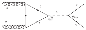
Figure 1: Feynman diagram of the dominant Higgs boson production at LHC with its subsequent FCSI decay into $\tau\mu$ pair.

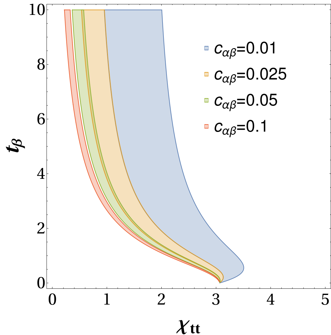
Figure 2: The colored areas in the $\chi_{tt}-t_{\beta}$ plane represent points agree with the $htt$ SM coupling including uncertainties coming from the top quark mass.

We use experimental data in order to constrain the free parameters previously mentioned. The software used for this propose is a Mathematica package called SpaceMath Arroyo-Ureña et al. (2022). The physical observables used to bind the free model parameters are listed below.

1. LHC Higgs boson data,

2. $B_{s}^{0}\to\mu^{-}\mu^{+}$ decay Workman et al. (2022),

3. Upper limits on the $\mathcal{BR}(\tau\to 3\mu)$ and $\mathcal{BR}(\tau\to\mu\gamma$) decays Workman et al. (2022),

4. Upper limit on the $\mathcal{BR}(h\to\tau\mu)$ decay Sirunyan et al. (2018a); Aad et al. (2020a),

5. The muon anomalous magnetic dipole moment $\delta a_{\mu}$ Abi et al. (2021),

6. Direct searches for additional heavy neutral $\mathcal{CP}$-even and $\mathcal{CP}$-odd scalars through $gb\to\phi\to\tau\tau$ ($\phi=\,H,\,A$) process are used to constrain their masses  Aaboud et al. (2018a); Sirunyan et al. (2018b). We denote them as $m_{H}$, $m_{A}$, respectively.

7. As far as the charged scalar mass $m_{H^{\pm}}$ is concerned, the observables to constrain $m_{H}^{\pm}$ are i) the upper limit on $\sigma(pp\to tbH^{\pm})\times\mathcal{BR}(H^{\pm}\to\tau^{\pm}\nu)$ Aaboud et al. (2018b) and ii) the decay $b\to s\gamma$ Chetyrkin et al. (1997); Adel and Yao (1994); Ali and Greub (1995); Greub et al. (1996); Ciuchini et al. (1998); Misiak and Steinhauser (2017).

III.1.1 Constraint on $c_{\alpha\beta}$ and $t_{\beta}$

We first analyze the impact of LHC Higgs boson data on $c_{\alpha\beta}$ and $t_{\beta}$. More precisely, we use the coupling modifiers $\kappa$-factors reported by ATLAS and CMS collaborations Aad et al. (2020b); Sirunyan et al. (2019). In the context of 2HDM-III, this observable is defined as follows

$$\kappa_{pp}^{2}=\frac{\sigma(pp\to h^{\text{2HDM-III}})}{\sigma(pp\to h^{\text{SM}})}\;\text{or}\;\kappa_{x\bar{x}}^{2}=\frac{\Gamma(h^{\text{2HDM-III}}\to X)}{\Gamma({h^{\text{SM}}}\to X)}.$$ (9)

In Eq. (9), $\Gamma(\phi_{i}\to X)$ is the decay width of $\phi_{i}=h^{\text{2HDM-III}}$, $h^{\text{SM}}$ into $X=b\bar{b},\,\tau^{-}\tau^{+},\,ZZ,\,WW,\,\gamma\gamma$, $gg$. Here $h^{\text{2HDM-III}}$ corresponds the SM-like Higgs boson coming from 2HDM-III and $h^{\text{SM}}$ stands for the SM Higgs boson; $\sigma(pp\to\phi_{i})$ is the Higgs boson production cross section through proton-proton collisions. Figure 3 shows colored areas corresponding to the allowed regions by each channel $X$. As far as the observables $h\to\tau\mu$, $\delta a_{\mu}$, $\tau\to 3\mu$, $\tau\to\mu\gamma$ and $B_{s}^{0}\to\mu^{-}\mu^{+}$ are concerned, we present in Figure 3 the area in accordance with experimental bounds. Meanwhile, Figure 3 displays the region consistent with all constrains. We also include the projections for HL-LHC and HE-LHC for Higgs boson data Cepeda et al. (2019) and for the decay $B_{s}^{0}\to\mu^{+}\mu^{-}$ Aad et al. (2020a).

Once we consider all the observables, we find strong restrictions for the 2HDM-III parameter space on the $c_{\alpha\beta}-t_{\beta}$ plane, in particular we observe that $c_{\alpha\beta}=0.05$ admits values for $t_{\beta}\approx 2$, $t_{\beta}\approx 8$, $t_{\beta}\approx 10$ for HE-LHC, HL-LHC and LHC, respectively. A special case, the alignment limit, i.e., $c_{\alpha\beta}\approx 0$ allows $t_{\beta}\approx 12,\,11,\,8$ for the LHC, HL-LHC and HE-LHC, respectively. A fact to highlight is that the 2HDM-III is able to accommodate the current discrepancy between the experimental measurement and the theoretical SM prediction of the muon anomalous magnetic dipole moment $\delta a_{\mu}$. However, from Figure 3, we observe that the allowed region by $\delta a_{\mu}$ is out of the intersection of the additional observables. This happens by choosing the parameters shown in Table 2. We find that $\delta a_{\mu}$ is sensitive to the parameter changing flavor $\chi_{\tau\mu}$ which was fixed to the unit in order to obtain the best fit of the 2HDM-III parameter space. Under this choice, $\delta a_{\mu}$ is explained with high values of $t_{\beta}$.

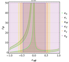
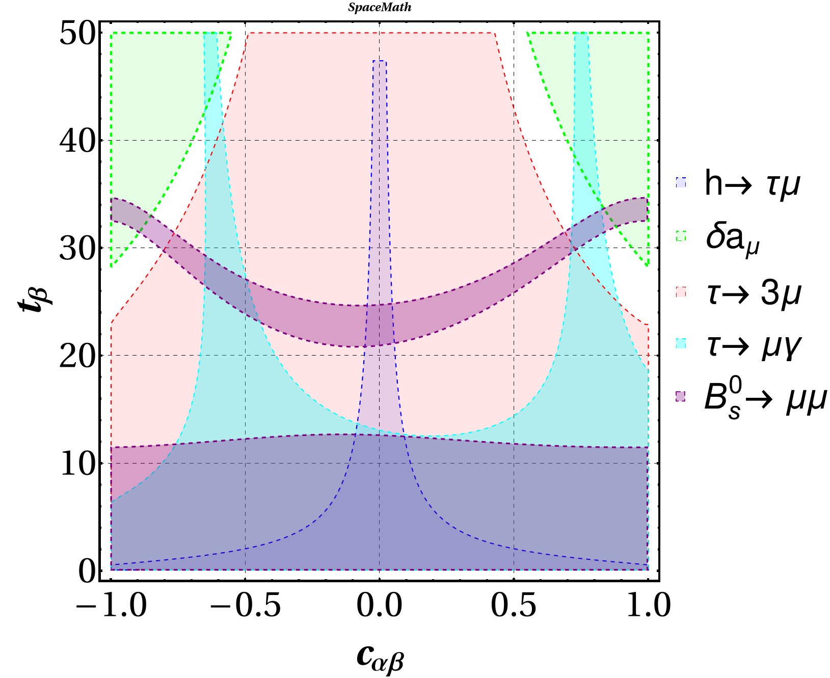
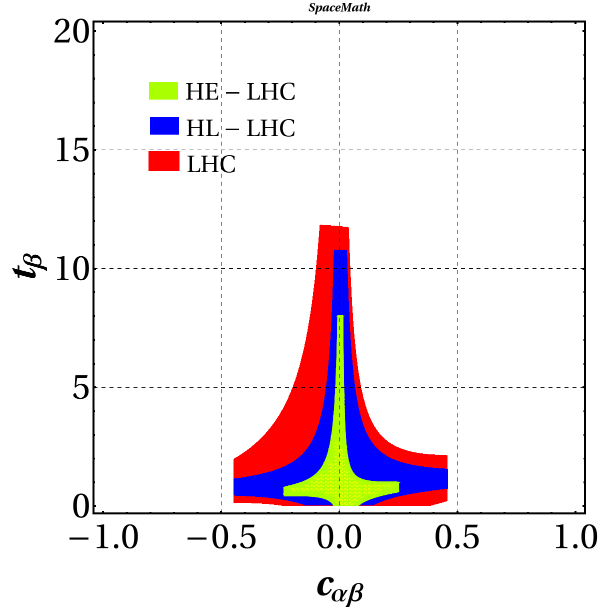
Figure 3: The shadowed areas represent the allowed regions in the plane $c_{\alpha\beta}$-$t_{\beta}$: (a) Coupling modifiers $\kappa$-factors, (b) $h\to\tau\mu$, $\delta a_{\mu}$, $\tau\to 3\mu$, $\tau\to\mu\gamma$ and $B_{s}^{0}\to\mu^{+}\mu^{-}$, (c) Intersection of all allowed regions. We have also included projections for HL-LHC and HE-LHC.

III.1.2 Constraint on $m_{H}$ and $m_{A}$

The ATLAS and CMS collaborations reported results of a search for hypothetical neutral heavy scalar and pseudoscalar bosons in the ditau decay channel Aaboud et al. (2018a); Sirunyan et al. (2018b). The search was done through the process $gb\to\phi\to\tau\tau$, where $\phi=A,\,H$ (see Fig. 4). Nevertheless, no significant deviation was observed from the predicted SM background, but upper limits on the production cross section $\sigma(gb\to\phi)$ times branching ratio $\mathcal{BR}(\phi\to\tau\tau)$ were imposed.

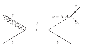
Figure 4: Feynman diagram of the production of $\phi$ in association with a bottom quark at LHC, with a subsequent decay into $\tau\tau$ pair.

Figure 5(a) shows the $\sigma(gb\to Hb)\times\mathcal{BR}(H\to\tau\tau)$ as a function of $m_{H}$ for illustrative values of $t_{\beta}=5,\,8,\,40$ and $c_{\alpha\beta}=0.01$, while in Figure 5(b) we present the same process but as a function of $m_{A}$ for $t_{\beta}=8,\,30,\,40$. The red crosses and black points correspond to the observed and expected values at 95$\%$ C.L., respectively. The green (yellow) band represents the interval at $\pm 1\sigma$ ($\pm 2\sigma$) according to the expected value. We implement the Feynman rules in CalcHEP Belyaev et al. (2013) to evaluate such a process.

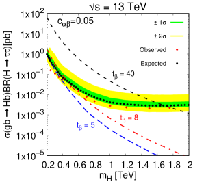
(a)

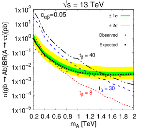
(b)

Figure 5: The observed and expected at 95$\%$ CL upper limits on the production cross section times ditau branching ratio for a scalar boson produced via $b$-associated production as a function of (a) the $\mathcal{CP}$-even mass for $t_{\beta}=$5, 8, 40 and (b) the $\mathcal{CP}$-odd mass for $t_{\beta}=$ 8, 30, 40. We take $c_{\alpha\beta}=0.05$.

From Figure 5(a) we can notice that $m_{H}\lesssim 500$ GeV ($m_{H}\lesssim 700$ GeV) are excluded at 1$\sigma$ (2$\sigma$) when $t_{\beta}=8$, while for $t_{\beta}\lesssim 5$ the upper limit on $\sigma(gb\to\phi b)\times\mathcal{BR}(\phi\to\tau\tau)$ is easily accommodated. Despite $t_{\beta}=$40 is ruled out (see Figure 3), we include it to illustrate the consistency (in the high mass regime) with the results reported in previous section. As far as the pseudoscalar mass is concerned, from Figure 5(b), we find that $m_{A}\lesssim$ 600 GeV ($m_{H}\lesssim$ 700 GeV) are excluded at 1$\sigma$ (2$\sigma$) for $t_{\beta}=8$.

III.1.3 Constraint on the charged scalar mass $m_{H^{\pm}}$

The detection of a charged scalar $H^{\pm}$ would represents a clear signature of new physics. Constraints were obtained from collider searches for the $H^{\pm}$ production and its subsequent decay into a $\tau^{\pm}\nu_{\tau}$ pair Aaboud et al. (2018b). More recently the ATLAS collaboration reported a study on the charged Higgs boson produced either in top-quark decays or in association with a top quark. Subsequently the charged Higgs boson decays via $H^{\pm}\to\tau^{\pm}\nu_{\tau}$ with a center-of-mass energy of 13 TeV Aaboud et al. (2018b). However, we find that such processes are not a good way to constrain the charged scalar mass $m_{H^{\pm}}$ predicted in 2HDM-III. Nevertheless, the situation is opposite if one consider the decay $b\to s\gamma$ which imposes severe lower limits on $m_{H^{\pm}}$ because to the charged boson contribution Ciuchini et al. (1998); Misiak and Steinhauser (2017).

Figure 6 shows the ratio $R_{quark}$ as a function of the charged scalar boson mass for $t_{\beta}=2,5,10$. Here, $R_{quark}$ is given by:

$$R_{quark}=\frac{\Gamma(b\to X_{s}\gamma)}{\Gamma(b\to X_{c}e\nu_{e})}.$$ (10)

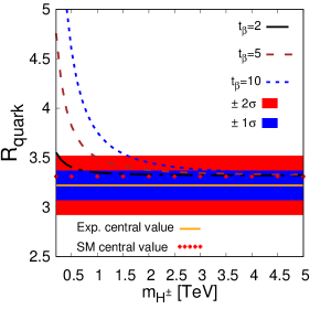
Figure 6: $R_{quark}$ at NLO in QCD as a function of the charged scalar boson mass for $t_{\beta}=$2, 5, 10. Solid line represents the experimental central value while red area indicate the theoretical SM, around the central value. Blue and red bands stand for 1$\sigma$ and 2$\sigma$, respectively. $R_{quark}$ is defined in Eq. 10.

When $t_{\beta}=2$, we notice that the charged scalar boson mass $100\,\text{GeV}\lesssim m_{H^{\pm}}$ ($700\,\text{GeV}\lesssim m_{H^{\pm}}$) is ruled out, at $2\sigma$ ($1\sigma$). The intermediate value $t_{\beta}=5$, excludes masses $800\,\text{GeV}\lesssim m_{H^{\pm}}$ ($2\,\text{TeV}\lesssim m_{H^{\pm}}$). Meanwhile, $t_{\beta}=10$ imposes a stringent lower bound $1.6\,\text{TeV}\lesssim m_{H^{\pm}}$ ($3.2\,\text{TeV}\lesssim m_{H^{\pm}}$).

In summary, we present in Table 2 the values used in the subsequent calculations.

Table 2: Values of the parameters used in the calculations.

Parameter	Value
$c_{\alpha\beta}$	0.01
$t_{\beta}$	0.1-8
$\chi_{\tau\mu}$	1
$m_{H}=m_{A}$	800 GeV

III.2 Collider analysis for $h\rightarrow\tau\mu$

In this section we simulate the production of the SM-like Higgs boson $h$ with its subsequent decay into a $\tau\mu$ pair at the LHC, HL-LHC, HE-LHC and FCC-hh. Let us first show in Figure 7, the branching ratio of the $h\to\tau\mu$ decay as a function of $t_{\beta}$ for $\chi_{\tau\mu}=0.1,\,0.5,\,1$ and $c_{\alpha\beta}=0.01$. We also include the upper limit reported by ATLAS and CMS collaborations ATL (2023); Sirunyan et al. (2021). We notice that for $\chi_{\tau\mu}=1$, values of $\tan\beta\leq 17$ are allowed, while $\chi_{\tau\mu}=0.5$ allows $\tan\beta\leq 35$, values of $\tan\beta\leq 50$ are admissible when $\chi_{\tau\mu}=0.1$.

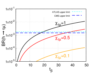
Figure 7: Branching ratio of the decay $h\to\tau\mu$ as a function of $t_{\beta}$ for $\chi_{\tau\mu}=0.1,\,0.5,\,1$. The horizontal line represents the upper limit on $\mathcal{BR}(h\to\tau\mu)$.

We analyze the LFV Higgs signal for the options of three cases corresponding to Future Hadron Colliders (FHC), namely: HL-LHC, HE-LHC and FCC-hh, with the following luminosities:

• FHC1: HL-LHC at a center-of-mass energy of 14 TeV and integrated luminosities 0.3 through 3 ab^-1,

• FHC2: HE-LHC at a center-of-mass energy of 27 TeV and integrated luminosities in the interval 0.3-12 ab^-1,

• FHC3: FCC-hh at a center-of-mass energy of 100 TeV and integrated luminosities from 10 to 30 ab^-1.

Once we have under control the free model parameters, as shown previously, we now turn to estimate the number of signal events produced in the three accelerator options.

Figure 8 shows the product of $\sigma(gg\to h)\mathcal{BR}(h\to\tau\mu)$ as a function of $t_{\beta}$ (left axis) and number of events (right axis) for FHC1, FHC2 and FHC3. The dark area indicates the allowed region by all observables analyzed previously (see Table 2). Given the center-of-mass energy and the integrated luminosity, we find that the maximum number of signal events produced, denoted by $\mathcal{N}_{\mathcal{S}}^{\textbf{FHCi}}$, are of the order $\mathcal{N}_{\mathcal{S}}^{\textbf{FHC1}}=\mathcal{O}(10^{5})$, $\mathcal{N}_{\mathcal{S}}^{\textbf{FHC2}}=\mathcal{O}(10^{6})$, $\mathcal{N}_{\mathcal{S}}^{\textbf{FHC3}}=\mathcal{O}(10^{7})$. Here, we consider $t_{\beta}=8$ and $\chi_{\tau\mu}=1$.

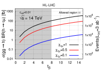
(a)

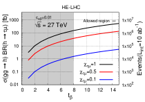
(b)

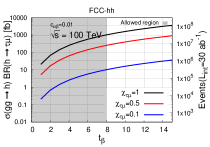
(c)

Figure 8: (a) Scenario SA, (b) Scenario SB, (c) Scenario SC. Left axis: $\sigma(gg\to h)\mathcal{BR}(h\to\tau\mu)$ as a function of $t_{\beta}$ for $\chi_{\tau\mu}$=0.1, 0.5, 1. Right axis: Events-$t_{\beta}$ plane. The dark area corresponds to the allowed region. See Table 2.

Let us now to analyze the signature of the decay $h\to\tau\mu$, with $\tau\mu=\tau^{-}\mu^{+}+\tau^{+}\mu^{-}$ and its potential SM background. The CMS and ATLAS collaborations Khachatryan et al. (2015); Aad et al. (2017) searched for this process through two $\tau$ decay channels: electron decay $\tau\to e\nu_{\tau}\nu_{e}$ and hadron decay $\tau_{h}\mu$. In this work, we will study the former. As far as our computation methods are concerned, we first implement the model in LanHEP Semenov (2016) for exporting the UFO files necessary to be interpreted in MadGraph5 Alwall et al. (2011), later it is interfaced with Pythia8 Sjostrand (2008) and Delphes 3 de Favereau et al. (2014) for simulates the response of the detector. Subsequently, we generate signal and background events, the last ones at NLO in QCD. We used NNPDF parton distribution functions Ball et al. (2017).

Signal and SM background processes

The signal and background processes are as following:

• SIGNAL- We search for a final state coming from the process $gg\to h\to\tau\mu\to e\nu_{\tau}\nu_{e}\mu$. This channel contains exactly two charged leptons, namely, one electron (or positron) and one antimuon (or muon) and missing energy because of undetected neutrinos.

• BACKGROUND- The potential SM background for the signal come from:

  1. Drell-Yan process, followed by the decay $Z\to\tau\tau\to e\nu_{\tau}\nu_{e}\mu\nu_{\tau}\nu_{\mu}$.

  2. $WW$ production with subsequent decays $W\to e\nu_{e}$ and $W\to\mu\nu_{\mu}$.

  3. $ZZ$ production, later decaying into $Z\to\tau\tau\to e\nu_{\tau}\nu_{e}\mu\nu_{\tau}\nu_{\mu}$ and $Z\to\nu\nu$.

Signal significance

The most restrictive kinematic cuts to separate the signal from the background processes are the collinear and transverse masses, $m_{\text{col}}$ and $M_{T}^{\ell}$, respectively. They are defined as following:

$$m_{\text{col}}(e\,\mu)=\dfrac{m_{\text{inv}}(e\,\mu)}{\sqrt{x}},\quad\text{with}\quad x=\dfrac{|\vec{P}_{T}^{e}|}{|\vec{P}_{T}^{e}|+\vec{E}_{T}^{\text{miss}}\cdot\vec{P}_{T}^{e}},$$ (11)

and

$$M_{T}^{\ell}=\sqrt{2|\vec{P}_{T}^{\ell}||\vec{E}_{T}^{\text{miss}}|(1-\cos\Delta\phi_{\vec{P}_{T}^{\ell}-\vec{E}_{T}^{\text{miss}}})}.$$ (12)

We present in Figure 9 the distribution of collinear mass of the signal events for the scenarios (a) FHC1, (b) FHC2 and (c) FHC3, We consider integrated luminosities of 3, 12 and 30 ab^-1 respectively, and $t_{\beta}$= 5, 8.

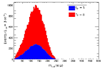
(a)

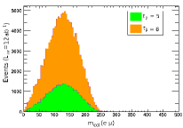
(b)

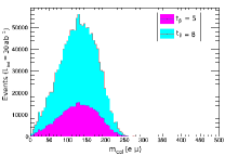
(c)

Figure 9: Distribution of the collinear mass for scenarios: (a) FHC1, (b) FHC2 and (c) FHC3.

For the kinematic analysis of the processes, we use the package MadAnalysis5 Conte et al. (2013). Besides the collinear mass and transverse mass, we applied additional cuts for both signal and background Aad et al. (2017); Khachatryan et al. (2015) as shown in Table 3 (scenario FHC1). Scenarios FHC1-FHC3 are available electronically in Kopp (2016). The number of the signal ($\mathcal{N}_{S}$) and background ($\mathcal{N}_{B}$) after the kinematic cuts were applied, are also included. We consider to the signal significance defined as $\mathcal{N}_{S}/\sqrt{\mathcal{N}_{S}+\mathcal{N}_{B}}$; once we compute it, the efficiency of the kinematic cuts for both signal and background are: $\epsilon_{S}\approx 0.13$ and $\epsilon_{B}\approx 0.014$, respectively.

Table 3: Kinematic cuts applied to the signal and main SM background for scenario $\mathbf{FHC1}$.

Cut number	Cut	$\mathcal{N}_{S}$	$\mathcal{N}_{B}$	$\mathcal{N}_{S}/\sqrt{\mathcal{N}_{S}+\mathcal{N}_{B}}$
	Initial (no cuts)	$5.77\times 10^{4}$	$2.00\times 10^{8}$	$4.10$
$1$	$|\eta^{e}|<2.3$	$2.53\times 10^{4}$	$1.30\times 10^{8}$	$2.20$
$2$	$|\eta^{\mu}|<2.1$	$1.64\times 10^{4}$	$1.07\times 10^{8}$	$1.59$
$3$	$0.1<\Delta R(e,\,\mu)$	$1.63\times 10^{4}$	$1.06\times 10^{8}$	$1.59$
$4$	$10<p_{T}(e)$	$1.55\times 10^{4}$	$3.90\times 10^{7}$	$2.49$
$5$	$20<p_{T}(\mu)$	$1.21\times 10^{4}$	$2.04\times 10^{7}$	$2.69$
$6$	$10<\text{MET}$	$1.12\times 10^{4}$	$2.01\times 10^{7}$	$2.50$
$7$	$100<m_{\text{col}}(e,\,\mu)<150$	$9.65\times 10^{3}$	$9.33\times 10^{6}$	$3.16$
$8$	$25<M_{T}(e)$	$8.67\times 10^{3}$	$4.83\times 10^{6}$	$3.95$
$9$	$15<M_{T}(\mu)$	$7.87\times 10^{3}$	$2.87\times 10^{6}$	$4.65$

In the previous analysis, we found that the LHC presents difficulties in carrying out an experimental scrutiny, achieving a statistical significance of $\sim 1.4\sigma$. However, more promising expectations arise at future stages of the LHC, namely, HL-LHC in which a prediction about $4.6\sigma$ for 3 ab^-1 and $t_{\beta}=8$ is found. Meanwhile, the HE-LHC (FCC-hh) offers exceptional results, we find a signal significance around $5.04\sigma$ ($\sim 5.43\sigma$) considering 9 ab^-1 and $t_{\beta}=6$ (15 ab^-1 and $t_{\beta}=3$). Then, we present in Fig. 10 regions for the model parameters corresponding to a potential evidence ($3\sigma$) or a possible discovery ($5\sigma$) for the three scenarios FHC1, FHC2, FHC3.

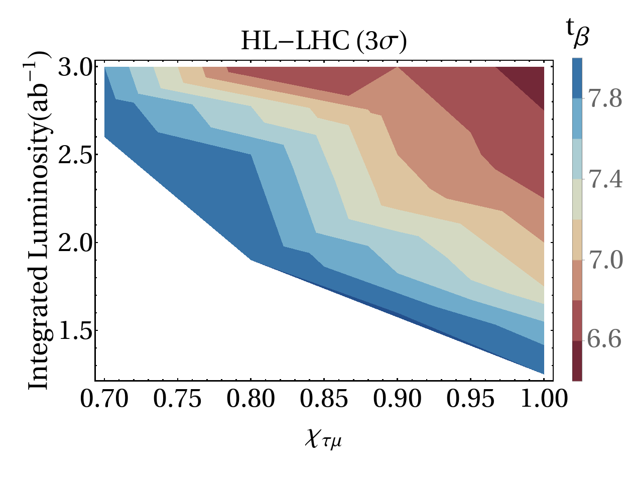
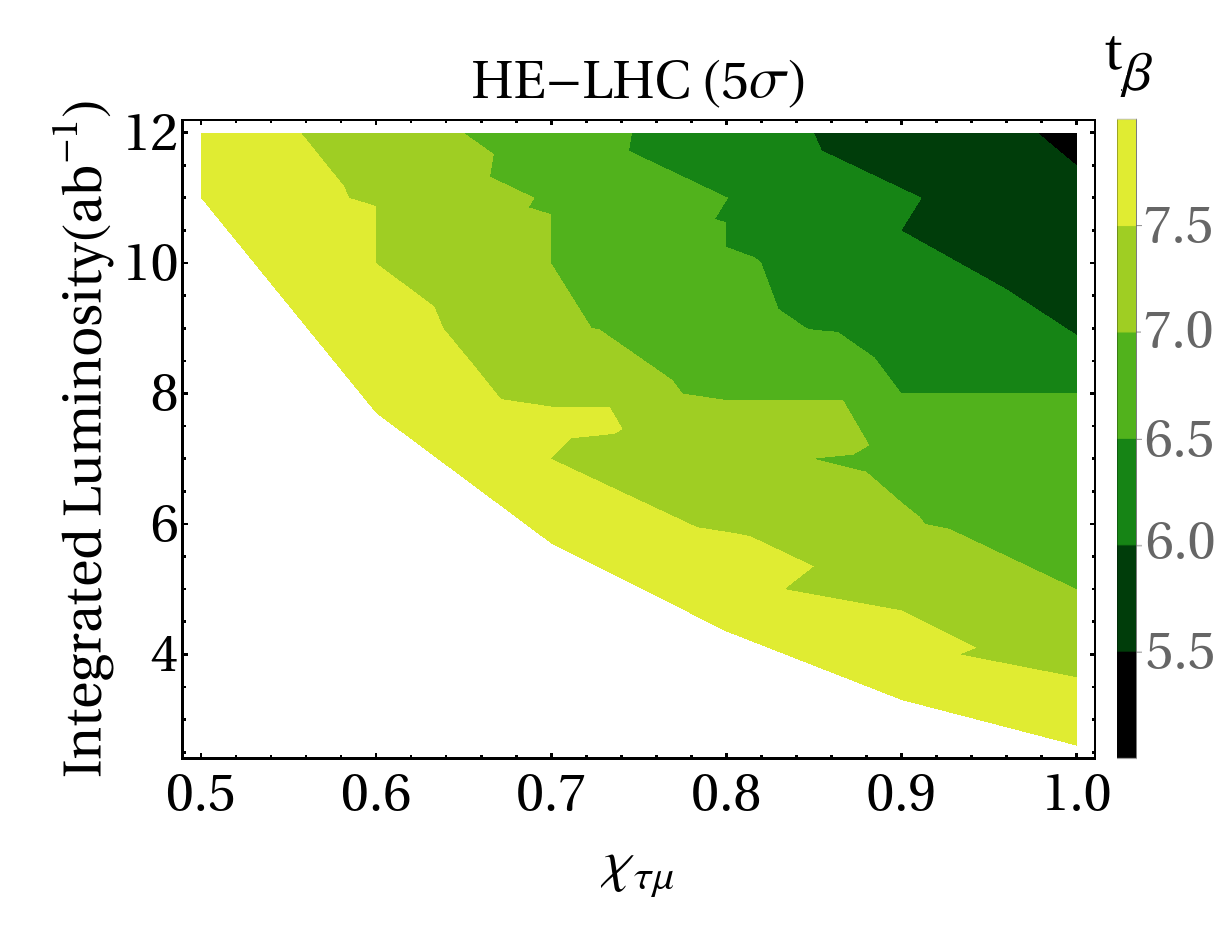
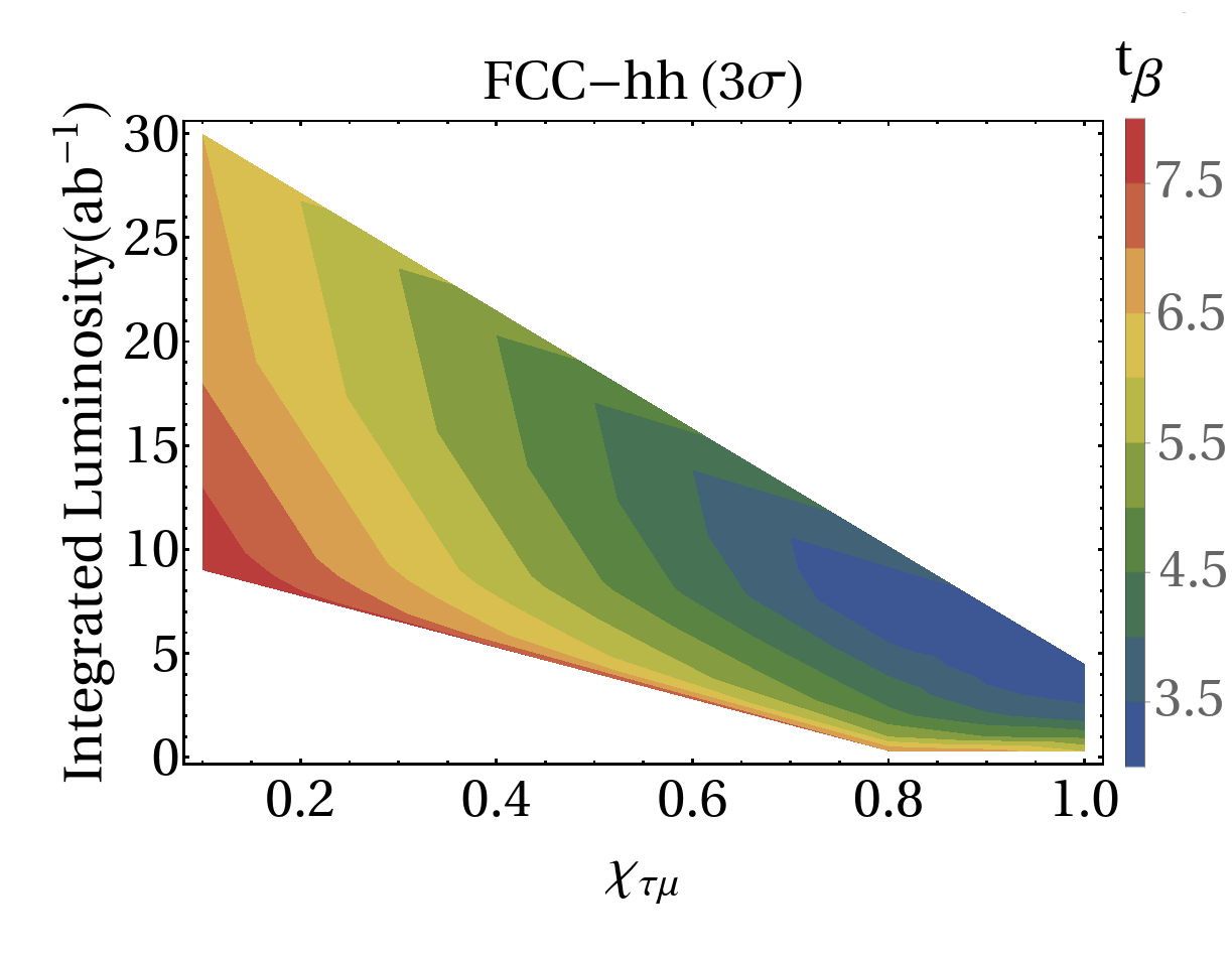
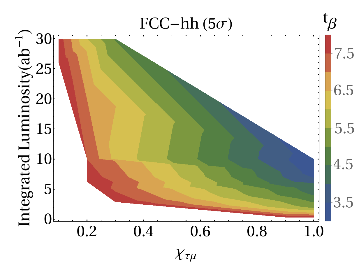
Figure 10: Signal significance as a function of the integrated luminosity, the $\chi_{\tau\mu}$ parameter of LFV coupling $h\tau\mu$ and $t_{\beta}$. (a), (b), (d): 3$\sigma$ and (c), (e): 5$\sigma$.

IV One-loop calculation of $h\to\ell_{a}\ell_{b}$ within 2HDM-I,II, with massive neutrinos

In the context of the 2HDM Type I and II, the interaction $h\ell_{a}\ell_{b}$ with $a\neq b$ is not allowed at tree level, because of all fermions interact with only one Higgs doublet, such as in the SM. However, considering neutrino masses the LFV-HD are induced at one loop by means of charged currents. Here, we consider the Inverse SeeSaw (ISS) mechanism to describe the lightness of neutrino masses Mohapatra (1986); Mohapatra and Valle (1986); Bernabéu et al. (1987), which is a natural extension of the type I and II variants of the 2HDM to include neutrino masses. In both versions of the 2HDM that we take into consideration here, the Yukawa term proportional to $\Phi_{2}$ is taken into account by the Dirac mass term for neutrinos. All fermions interact with $\Phi_{2}$ in type I, and up-type fermions (in this case, neutrinos) interact with $\Phi_{2}$ in type II.

In this work, we assume a normal hierarchy for light neutrino masses and we collect the experimental values for the neutrino oscillations parameters in the Table 4 Esteban et al. (2019).

	BFP $\pm 1\sigma$	$3\sigma$
$\sin^{2}{(\theta_{12})}$	$0.310^{+0.013}_{-0.012}$	$0.275-0.350$
$\sin^{2}{(\theta_{23})}$	$0.582^{+0.015}_{-0.019}$	$0.428-0.624$
$\sin^{2}{(\theta_{13})}$	$0.02240^{+0.00065}_{-0.00066}$	$0.02244-0.02437$
$\frac{\Delta m_{21}^{2}}{10^{-5}\text{eV}^{2}}$	$7.39^{+0.021}_{-0.020}$	$6.79-8.01$
$\frac{\Delta m_{31}^{2}}{10^{-5}\text{eV}^{2}}$	$2.525^{+0.033}_{-0.031}$	$2.431-2.622$

Table 4: Neutrino oscillations data for a normal hierarchy. The second column show the Best Fit Point (BFP) and the $1\sigma$ range, third column shows the $3\sigma$ range.

In the normal hierarchy, we can rewrite the masses of $\nu_{2,3}$ in terms of $m_{1}$, the mass of the lightest neutrino $\nu_{1}$, and the square mass differences as follows

$$m_{i}=\sqrt{m_{1}^{2}+\Delta m_{i1}^{2}},\quad i=2,3.$$ (13)

IV.1 The model $\nu$2HDM-I, II

In the Yukawa sector, we include three pairs of fermionic singlets ($\nu_{R}$, $X$) to the SM Arganda et al. (2015). The right handed neutrinos $\nu_{R}$ singlets partners of $\nu_{L}$ in the SM with lepton number $L=-1$, while the extra singlet $X$ has lepton number $L=1$. With these additional fermions, we can write the Lagrangian

$$\mathcal{L}^{\nu}=-Y_{ij}^{2,\nu}\overline{L_{i}}\tilde{\Phi}_{2}\nu_{Rj}-M_{ij}^{\nu}\overline{\nu_{Ri}^{C}}X_{j}-\frac{1}{2}\mu_{Xij}\overline{X_{i}^{C}}X_{j}+\textrm{H. c.},$$ (14)

where $i,j=1,2,3$, $Y^{\nu}_{2}$ is the $3\times 3$ neutrino Yukawa matrix associated to the $\Phi_{2}$ Higgs doublet, $M_{R}$ is a lepton number conserving complex $3\times 3$ matrix and $\mu_{X}$ is a Majorana complex $3\times 3$ symmetric mass matrix that violates the lepton number conservation by two units. Hence, the $9\times 9$ neutrino mass matrix after the electroweak symmetry breaking, in the $(\nu_{L},\nu_{Ri}^{C},X_{i}^{C})$ basis, is given by

$$M^{\nu}_{\text{ISS}}=\begin{pmatrix}0&m_{D}^{2}&0\\ m_{D}^{2,\top}&0&M_{R}\\ 0&M_{R}^{\top}&\mu_{X}\end{pmatrix},$$ (15)

where $m_{D}^{2}=\frac{v_{2}}{\sqrt{2}}Y^{2,\nu}$ is the Dirac matrix, which is symmetric then can be diagonalized by a $9\times 9$ unitary matrix $U_{\nu}$ given by

$$U_{\nu}^{T}M_{\mathrm{ISS}}^{\nu}U_{\nu}=\operatorname{diag}\left(m_{n_{1}},\ldots,m_{n_{9}}\right),$$ (16)

where $m_{n_{i}}$ are the masses of the nine physical Majorana neutrinos ${n_{i}}$ and are associated with the electroweak basis by the rotation

$$\left(\begin{array}[]{c}\nu_{L}^{C}\\ \nu_{R}\\ X\end{array}\right)=U_{\nu}P_{R}\left(\begin{array}[]{c}n_{1}\\ \vdots\\ n_{9}\end{array}\right),\quad\left(\begin{array}[]{c}\nu_{L}\\ \nu_{R}^{C}\\ X^{C}\end{array}\right)=U_{\nu}^{*}P_{L}\left(\begin{array}[]{c}n_{1}\\ \vdots\\ n_{9}\end{array}\right).$$ (17)

As a consequence of neutrino masses, following the notation of Aoki et. al. Aoki et al. (2009) and Diaz Lorenzo Díaz-Cruz (2019), the Yukawa Lagrangian in the leptonic sector is given by

$$\mathcal{L}^{2HDM}_{\text{Yuk,ISS}} =-\sum_{\ell}\left(\frac{m_{\ell}}{v}c_{h}^{\ell}\overline{\ell}\ell h+\frac{m_{\ell}}{v}c_{H}^{\ell}\overline{\ell}\ell H-i\frac{m_{\ell}}{v}e_{A}^{\ell}\overline{\ell}\gamma_{5}\ell A\right)$$

$$\quad-\dfrac{1}{v}\sum_{ij}^{9}\left(c^{n}_{h}\overline{n_{i}}(\omega_{ij}P_{R}+\omega_{ij}^{*}P_{L})n_{j}h+c^{n}_{H}\overline{n_{i}}(\omega_{ij}P_{R}+\omega_{ij}^{*}P_{L})n_{j}H-ie^{n}_{A}\overline{n_{i}}(\omega_{ij}P_{R}-\omega_{ij}^{*}P_{L})n_{j}A\right)$$

$$\quad-\left(\dfrac{\sqrt{2}U_{n\ell}}{v}\overline{n}(m_{n}e^{n}_{A}P_{L}+m_{\ell}e^{\ell}_{A}P_{R})\ell H^{+}+\text{H.c.}\right)$$

$$\quad-\left(\dfrac{\sqrt{2}U_{n\ell}}{v}\overline{n}(m_{n}P_{L}+m_{\ell}P_{R})\ell G^{+}+\text{H.c.}\right).$$ (18)

where $P_{L/R}$ are projections operators for left-/right-handed fermions. The second row of equation (18) was calculated in analogy with Thao et al. (2017) for the $\nu$SM model. Also, $\omega_{ij}=m_{n_{j}}C_{ij}+m_{n_{i}}C_{ij}^{*}$ and $C_{ij}=\sum_{c=1}^{3}U_{ci}^{\nu}U_{cj}^{\nu*}$. Finally, the $c_{\phi^{0}}^{f}$ ($\phi^{0}=h,H$) and $e_{A}^{f}$ factors for charged leptons and neutrinos are given in Table 5.

	Type I	Type II
$c_{h}^{\ell}$	$\cos{\alpha}/\sin{\beta}$	$-\sin{\alpha}/\cos{\beta}$
$c_{H}^{\ell}$	$\sin{\alpha}/\sin{\beta}$	$\cos{\alpha}/\cos{\beta}$
$e_{A}^{\ell}$	$-\cot{\beta}$	$t_{\beta}$
$c_{h}^{n}$	$\cos{\alpha}/\sin{\beta}$	$\cos{\alpha}/\sin{\beta}$
$c_{H}^{n}$	$\sin{\alpha}/\sin{\beta}$	$\sin{\alpha}/\sin{\beta}$
$e_{A}^{n}$	$\cot{\beta}$	$\cot{\beta}$

Table 5: Factors $c_{\phi^{0}}^{f}$ and $e_{A}^{f}$ in the $\nu$2HDM-I,II.

The neutral currents in the Lagrangian (18), can be rewritten following the notation of equation (3). For charged leptons, only the following $\mathcal{CP}$-conserving and $\mathcal{CP}$-violating factors are non-zero,

$$S^{\ell,\phi^{0}}=\frac{gm_{\ell}}{2m_{W}}c_{\phi^{0}}^{\ell};\qquad P^{\ell,A}=-\frac{gm_{\ell}}{2m_{W}}e_{A}^{\ell}\delta.$$ (19)

In the case of neutrinos, as a consequence of the ISS, $\mathcal{CP}$-conserving and $\mathcal{CP}$-violating factors appears,

$$S_{ij}^{n,\phi}=\frac{1}{2v}c^{n}_{\phi}(\omega_{ij}+\omega_{ij}^{*});\qquad P_{ij}^{n,\phi}=-\frac{i}{2v}c^{n}_{\phi}(\omega_{ij}-\omega_{ij}^{*}),$$ (20)

$$S_{ij}^{n,A}=-\frac{1}{2v}e^{n}_{A}(\omega_{ij}-\omega_{ij}^{*});\qquad P_{ij}^{n,A}=\frac{i}{2v}e^{n}_{A}(\omega_{ij}+\omega_{ij}^{*}).$$ (21)

As a result, the interaction of neutral scalars and leptons is given by

$$\mathcal{L}_{\phi ff} =-\sum_{\ell}\left(S^{\ell,h}\overline{\ell}\ell h+S^{\ell,H}\overline{\ell}\ell H+iP^{\ell,A}\overline{\ell}\gamma_{5}\ell A\right)$$ (22)

$$-\sum_{ij}^{9}\left(\overline{n_{i}}(S_{ij}^{n,h}+i\gamma_{5}P_{ij}^{n,h})n_{j}h+\overline{n_{i}}(S_{ij}^{n,H}+i\gamma_{5}P_{ij}^{n,H})n_{j}H+i\overline{n_{i}}(S_{ij}^{n,A}+i\gamma_{5}P_{ij}^{n,A})n_{j}A\right).$$ (23)

The LFV-HD are allowed at one-loop by means of charged currents mediated by $G^{\pm}$, $W^{\pm}$ and $H^{\pm}$. Detailed formulae for LFV-HD at one loop was presented in our previous paper Zeleny-Mora et al. (2022), with the decay width being written in terms of the form factors $A_{L,R}$, namely:

$$\Gamma(h\rightarrow\ell_{a}\ell_{b}) \equiv\Gamma(h\rightarrow\ell_{a}^{+}\ell_{b}^{-})+\Gamma(h\rightarrow\ell_{a}^{-}\ell_{b}^{+})$$

$$=\dfrac{1}{8\pi m_{h}}\left[1-\left(\frac{m_{a}^{2}+m_{b}^{2}}{m_{r}}\right)^{2}\right]^{1/2}\left[1-\left(\frac{m_{a}^{2}-m_{b}^{2}}{m_{r}}\right)^{2}\right]^{1/2}$$

$$\times\left[(m_{h}^{2}-m_{a}^{2}-m_{b}^{2})(|A_{L}|^{2}+|A_{R}|^{2})-4m_{a}m_{b}\text{Re}(A_{L}A^{*}_{R})\right].$$ (24)

The general topologies of Feynman graphs that contribute to the amplitude are shown in Figure 11, where S, F and V denote scalars, fermions and vectors, respectively. In the special case of the $\nu$2HDM-I,II, 18 Feynman graphs contributes to LFV-HD at one loop, summarized in Table 7, and the associated couplings are given in Table 6. We work in Feynman-tHooft gauge and use dimensional regularization to manage the divergences. The analytical expressions for the form factors of each diagram are presented in the Appendix A. The result for the form factors is finite, i.e., free of divergences, as it should be considering that the LFV Higgs couplings do not exist at tree-level.

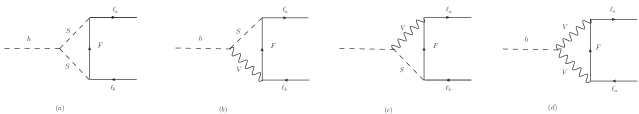
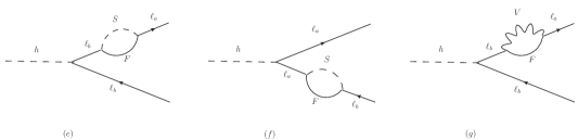
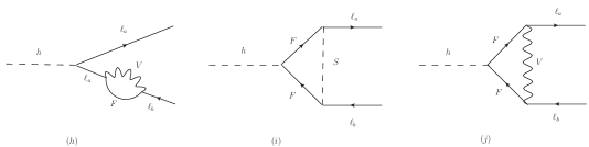
Figure 11: Feynman diagrams that contribute at one-loop level to the $h\to\ell_{a}\ell_{b}$ decay in the 2HDM-I and II  Zeleny-Mora et al. (2022). Here $F,S,V$ represent fermion, scalar and vector contributions, respectively.

IV.2 Numerical analysis and results

The ISS mechanism explain the smallness of neutrino masses, assuming the hierarchy, $|\mu_{X}|\ll|M_{D}|\ll|M_{R}|$, by means of

$$\hat{m}_{\nu}\approx M_{D}^{2}M^{\top-1}_{R}\mu_{X}M^{-1}_{R}M_{D}^{2,\top},$$ (25)

where $\mathcal{M}=M^{\top-1}_{R}\mu_{X}M^{-1}_{R}$. On one hand, the mass matrix for light neutrinos (25) is proportional to $\mu_{X}$ and inversely proportional to $M_{R}$. On the other hand, (25) has the usual form in the SeeSaw (SS) type I mechanism. Then, considering the flavor basis, where the Yukawa matrix for charged leptons, $Y^{\ell}$, the mass matrices $M_{R}$ , $\mu_{X}$, and the gauge interactions are diagonal, as a consequence, the Dirac mass matrix $M_{D}^{2}$ can be rewritten in terms of 9 neutrino masses, the leptonic mixing matrix $U_{\text{PMNS}}$ and an $3\times 3$ orthogonal matrix $Q$ as follows Casas and Ibarra (2001):

$$M_{D}^{2}=\left(\widehat{\mathcal{M}}\right)^{1/2}Q\left(\widehat{m}_{\nu}\right)^{1/2}U_{\mathrm{PMNS}}^{\dagger},$$ (26)

where $\widehat{m}_{\nu}=\text{diag}(m_{n_{1}},m_{n_{2}},m_{n_{3}})$ and $\widehat{\mathcal{M}}=\text{diag}(m_{n_{4}},\dots,m_{n_{9}})$. Although, in general the matrix $Q$ depends on three complex angles, in this work, we chose $Q$ as the identity matrix, also, we assume that $M_{R}=\text{diag}(M_{R1},M_{R2},M_{R3})$ and $\mu_{X}=\text{diag}(\mu_{X1},\mu_{X2},\mu_{X3})$. As a result, $M_{D}^{2}$ depends only on neutrino masses and the mixing matrix $U_{\text{PMNS}}$. The last one could be calculated using the BFP values from Table 4. The 9 neutrino masses are reduced to 6 by means of equation (13) and assuming $m_{n_{1}}=10^{-12}$ GeV. To simplify the numerical analysis we consider degenerate values to $M_{R1}=M_{R2}=M_{R3}=M_{R}$ and $\mu_{X1}=\mu_{X2}=\mu_{X3}=\mu_{X}$.

IV.2.1 Constraint on the THDM-I and THDM-II

We now turn to analyze the THDM-I and THDM-II parameter space

• Signal strength modifiers: We consider the use of signal strength modifiers $\mathcal{R}_{X}$ for constraint the parameter space. For a production process $\sigma(pp\to\phi_{i})$ and the decay $\phi_{i}\to X$, $\mathcal{R}_{X}$ is defined as follows

  $$\mathcal{R}_{X}=\frac{\sigma(pp\to h)\mathcal{BR}(h\to X)}{\sigma(pp\to h^{\text{SM}})\mathcal{BR}(h^{\text{SM}}\to X)},$$ (27)

  with $\phi_{i}=h,\,h^{\text{SM}}$, where $h$ stands for the SM-like Higgs boson coming from an extension of the SM and $h^{\text{SM}}$ is the SM Higgs boson; $\mathcal{BR}(\phi_{i}\to X)$ is the rate of the $\phi_{i}\to X$ decay, with $X=b\bar{b},\,\tau^{-}\tau^{+},\,\mu^{-}\mu^{+},\,W^{+}W^{-},\,ZZ,\,\gamma\gamma$. Figure 12 shows the $\cos(\alpha-\beta)-\tan\beta$ plane for the case of 12(a) THDM-I and 12(b) THDM-II.

  

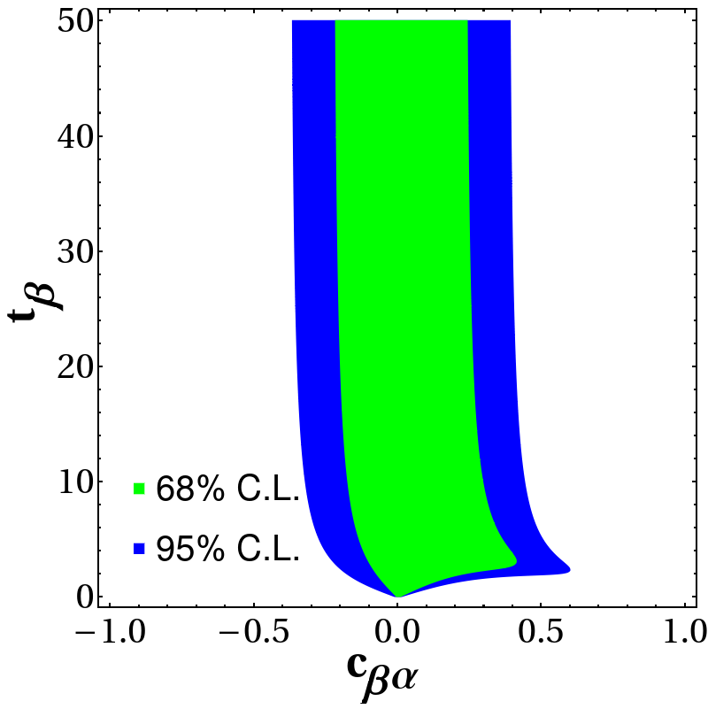
  (a)

  

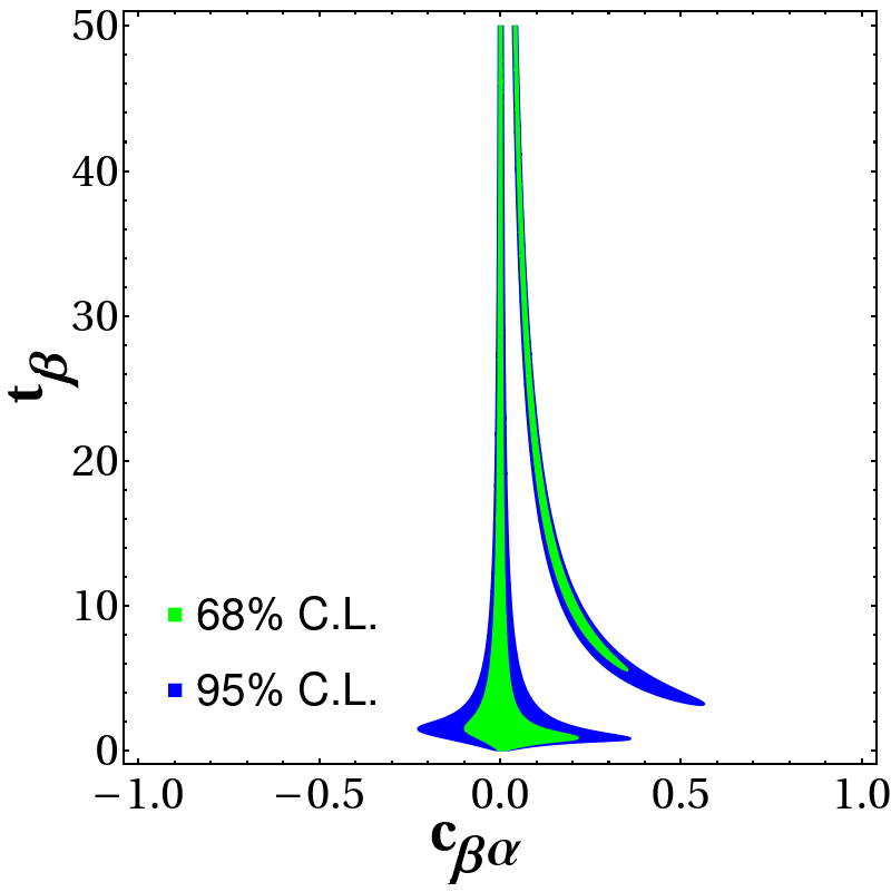
  (b)

  Figure 12: The $c_{\beta\alpha}-t_{\beta}$ shows the allowed areas by LHC Higgs boson data. Green (Blue) area stands for 68% (95%) of confidence level.

• Perturvativity: This bound applies over Yukawa matrix and implies that $|Y^{2,\nu}_{ij}|^{2}<6\pi$ Arganda et al. (2015); Thao et al. (2017). If we include the factor $(v_{2}/\sqrt{2})^{2}$, we obtain a bound for the Dirac matrix, given by:

  $$|(M_{D}^{2})_{ij}|^{2}<3\pi v_{2}^{2}=3\pi v^{2}\sin(\beta)^{2}.$$ (28)

  In the framework that we considered (26) depends on $M_{R}$ and $\mu_{X}$ and $\tan{\beta}$, then, the perturvativity bound (28) constraints this parameters as shown in the Figure 13.

  

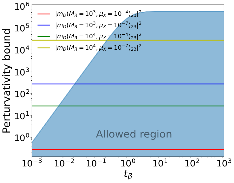
  Figure 13: Perturvativity bound on the $(M_{D}^{2})_{23}$ in the $\nu$2HDM-I,II. The blue region represents the allowed perturvativity space, see Eq. (28).

IV.3 Events for the $h\to\mu\tau$ decay at future hadron colliders

For the numerical evaluation, we observe that $\mathcal{BR}(h\to\ell_{a}\ell_{b})$ depends on the scales of neutrino masses $M_{R}$ and $\mu_{X}$, the parameters $\tan{\beta}$ and $\cos{\beta-\alpha}$, the masses $m_{H^{\pm}}$, $m_{A}$ and $\lambda_{5}$. From the signal strength modifiers, we can observe that the parameter space is in agreement with the alignment limit $\beta-\alpha=\frac{\phi}{2}$ or $c_{\beta\alpha}=0$. However, we assume in this work a quasi-alignment value of $c_{\beta\alpha}=0.01$. Also, we use, $M_{R}=1$ TeV, $m_{A}=587$ GeV, $\lambda_{5}=2.167$.

The branching ratio of $\mathcal{BR}(h\to\mu\tau)$ is shown in Figure 14, as function of $\tan{\beta}$ and $m_{H^{\pm}}$ for type I and II $\nu$2HDM, considering two cases for $\mu_{X}=10^{-4},10^{-7}$. In Figure13, for the case of $\mu_{X}=10^{-4}$ (red dashed line) the perturvativity bound does not constraint the values of $t_{\beta}$, however for the case of $\mu_{X}=10^{-7}$ (blue dashed line), the allowed values are $t_{\beta}\gtrsim 5\times 10^{-1}$.

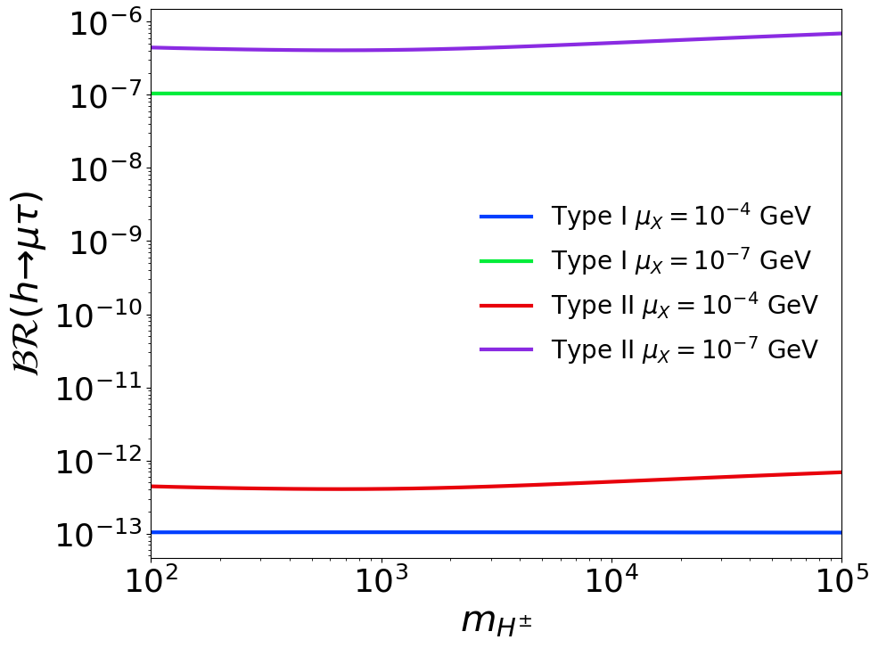
(a)

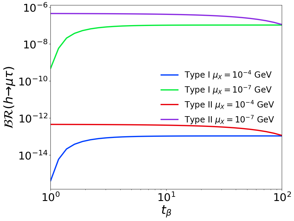
(b)

Figure 14: Behavior of branching ratio of $h\to\mu\tau$. In the left panel we show the $\mathcal{BR}(h\to\mu\tau)$ vs $m_{H^{\pm}}$ with $t_{\beta}=10$. In the right panel, we show $\mathcal{BR}(h\to\mu\tau)$ vs $t_{\beta}$ with $m_{H^{\pm}}=600$ GeV.

On one hand, in Figure 14(a), we observe that $\mathcal{BR}(h\to\mu\tau)$ is sensible to the scale of $m_{H^{\pm}}$ for the type II. In contrast to type I, where the dependence on $m_{H^{\pm}}$ disappear. Only the couplings $hH^{\pm}G^{\mp}$ and $hH^{\pm}H^{\mp}$ contain explicit dependence on $m_{H^{\pm}}$, see Table 6, which appears in diagrams 14, 15 and 16 on Table 7. However, these contributions are not dominant, and as a consequence the weak dependence on $m_{H^{\pm}}$, the difference in type I and II comes from the values of $\xi_{h}^{\ell}$ and $\xi_{A}^{\ell}$. On the other hand, in Figure 14(b) we observe a dependency over $t_{\beta}$ in both version of $\nu$2HDM. In the type I, $\mathcal{BR}(h\to\mu\tau)$ is small for $t_{\beta}$ close to 1 and increase with $t_{\beta}$ up to $t_{\beta}\approx 5$, to reach a constant value. Conversely, for type two the behavior is reversed, when $t_{\beta}$ is close to 1, we observe a constant value $\mathcal{BR}(h\to\mu\tau)$ and for values near to $t_{\beta}=10^{2}$, the $\mathcal{BR}(h\to\mu\tau)$ decrease. Although, in both models, the neutrinos couple to the same Higgs doublet ($\Phi_{2}$), the charged leptons do not. The form of $\mathcal{BR}(h\to\mu\tau)$ in type I and II models shown in Figure 14 its on the values of $\xi_{h}^{\ell}$ and $\xi_{A}^{\ell}$. Lastly, in both models the $\mathcal{BR}(h\to\mu\tau)$ shows a dependency on $\mu_{X}$ scale, as a consequence of the Casas-Ibarra parametrization (26).

Similarly to Section III.2, we show the number of Events-$t_{\beta}$ in the Figure 15, considering the production cross section $\sigma(pp\to h\to\tau\mu)=\sigma(gg\to h)\mathcal{BR}(h\to\tau\mu)$ for scenarios FHC1, FHC2 and FHC3. The dark area indicates the allowed region by all observables analyzed previously (see Table 2). Given the center-of-mass energy and the integrated luminosity, we find that the maximum number of signal events produced are of the order $\mathcal{N}_{\mathcal{S}}^{\textbf{FHC1}}=\mathcal{O}(10^{2})$, $\mathcal{N}_{\mathcal{S}}^{\textbf{FHC2}}=\mathcal{O}(10^{3})$, $\mathcal{N}_{\mathcal{S}}^{\textbf{FHC3}}=\mathcal{O}(10^{4})$, for $\nu$2HDM-II and $\mu_{X}=10^{-7}$ GeV.

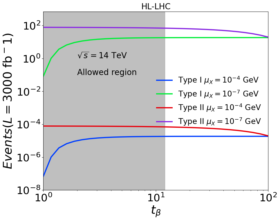
(a)

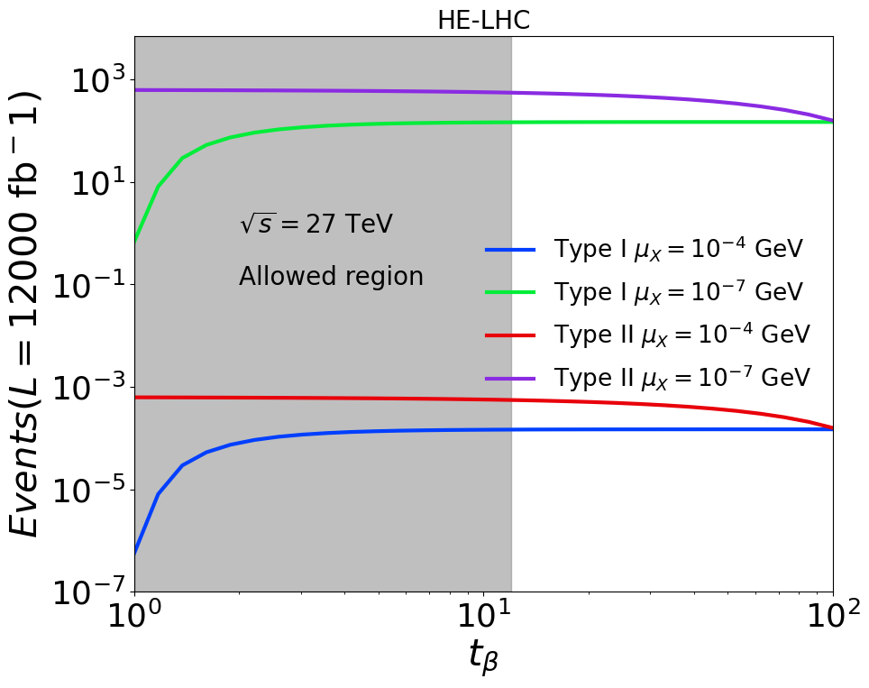
(b)

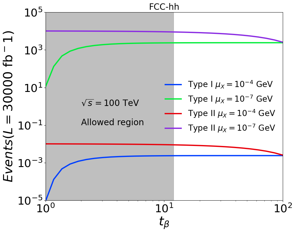
(c)

Figure 15: Events-$t_{\beta}$ plane, for (a) Scenario FCH1, (b) Scenario FCH2, (c) Scenario FCH3. The dark area corresponds to the allowed region. See Table 2.

V Conclusions

We have presented a general discussion of the search for the LFV Higgs decays at LHC, including several versions of the 2HDM, namely: the texturized version (2HDM-Tx), which is a particular version of the general model 2HDM-III, as well as the 2HDM with neutrino masses based on the inverse see-saw mechanism ($\nu$2HDM). For the 2HDM-Tx we started by deriving the constraints on the model parameters, and the lessons that LHC can give on the model structure. This was followed by the presentation of our study for the limits on $\mathcal{BR}(h\to\tau\mu)$ that can be achieved at LHC, as a function of the integrated luminosities that are projected for the future phases of the LHC. Then, we also discuss the expected rates for the LFV decay $h\to\ell_{a}\ell_{b}$, within the $\nu$2HDM, where such coupling is induced at one-loop level, with some technical details left for the appendix A. These results are summarized in the figure 16. There we can see that current limits from ATLAS and CMS on $\mathcal{BR}(h\to\tau\mu)$ are getting quite close to the value $10^{-3}$. Thus, values of the parameter $\chi_{\tau\mu}$ of order $1$ $(0.5)$ are excluded for values of $t_{\beta}$ larger than about $20$ $(35)$. However, we can also see that for $t_{\beta}=8$, $c_{\alpha\beta}=0.01$, values of $\chi_{\tau\mu}=0.5$ imply values of $\mathcal{BR}(h\to\tau\mu)$ about $10^{-4}$, which are still consistent with current limits, but could be rule out in searches for future eletron-positron colliders.

On the other hand, for the loop-induced LFV Higgs decay, we find that $\mathcal{BR}(h\to\tau\mu)$ is about $10^{-7}$ for the version $\nu$2HDM-I, and $10^{-13}$ for the version $\nu$2HDM-II, which are still far from the experimental reach of LHC and future colliders.

Thus, we have learned from LHC that models with large tree-level LFV Higgs couplings, as arising in the 2HDM-III, are being constrained by current data, but even the model version with textures (2HDM-Tx) has regions of parameters that pass current constraints. The coming phases of LHC with higher luminosity will be able to probe models where such LFV Higgs couplings arise at tree-level, but include a suppression mechanism, as in MFV or BGL models Branco et al. (1996b). Finally, we conclude that models where such couplings arise at loop-level, as in the MSSM or 2HDM with neutrino masses, seem to be out of the reach of LHC14.

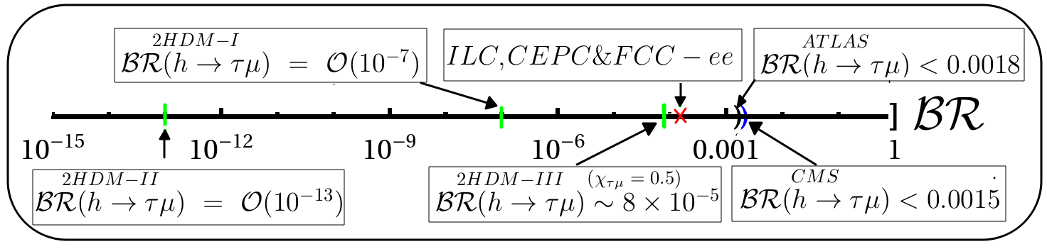
Figure 16: Comparison between experimental results (and projections) and our predictions for the $\mathcal{BR}(h\to\tau\mu)$. We have considered $t_{\beta}=8$ and $c_{\beta\alpha}=0.01$ in the numerical evaluation.

Acknowledgments

The work of Marco A. Arroyo-Ureña is supported by “Estancias posdoctorales por México (CONAHCYT)” and “Sistema Nacional de Investigadores” (SNI-CONAHCYT). JLD-C and O.F.B. acknowledge the support of SNI-CONAHCYT and VIEP (BUAP). M. Zeleny thanks Conacyt for the doctoral grant.

Appendix A Scalar couplings for LFV-HD and form factors

We present the couplings of SM-like Higgs and charged currents in Table 6. In this case we use the quiral notation in agreement with Zeleny-Mora et al. (2022).

Vertex	Coupling	Vertex	Coupling
$hW^{+}W^{-}$	$igm_{W}\Xi_{h}$	$hG^{+}G^{-}$	$-i\dfrac{gm_{h}^{2}\Xi_{h}}{2m_{W}}$
$hG^{+}W^{-}$	$i\dfrac{g\Xi_{h}}{2}(p_{+}-p_{0})_{\mu}$	$hW^{+}G^{-}$	$i\dfrac{g\Xi_{h}}{2}(p_{0}-p_{-})_{\mu}$
$hH^{+}W^{-}$	$i\dfrac{g\eta_{h}}{2}(k_{+}-p_{0})_{\mu}$	$hW^{+}H^{-}$	$i\dfrac{g\eta_{h}}{2}(p_{0}-k_{-})_{\mu}$
$hH^{\pm}G^{\mp}$	$i\dfrac{g\eta_{h}(m_{H^{\pm}}^{2}-m_{h}^{2})}{2m_{W}}$	$hH^{\pm}H^{\mp}$	$ig\dfrac{\rho_{h}\mathcal{K}_{h}-\Delta_{h}\mathcal{Q}_{h}}{4m_{W}\sin{2\beta}}+i\dfrac{4\lambda_{5}m_{W}\rho_{h}}{g\sin{2\beta}}$
$hl\overline{l}$	$-igc_{h}^{l}\dfrac{m_{l}}{2m_{W}}$	$hn_{i}n_{j}$	$\dfrac{-igc^{n}_{h}}{2m_{W}}\left[C_{ij}\left(P_{L}m_{n_{i}}+P_{R}m_{n_{j}}\right)+C_{ij}^{*}\left(P_{L}m_{n_{j}}+P_{R}m_{n_{i}}\right)\right]$
$\bar{n}_{i}\ell_{a}W_{\mu}^{+}$	$\dfrac{ig}{\sqrt{2}}U_{ai}^{\nu}\gamma^{\mu}P_{L}$	$\overline{\ell_{a}}n_{j}W_{\mu}^{-}$	$\dfrac{ig}{\sqrt{2}}U_{aj}^{\nu*}\gamma^{\mu}P_{L}$
$\bar{n}_{i}\ell_{a}G_{W}^{+}$	$-\dfrac{ig}{\sqrt{2}m_{W}}U_{ai}^{\nu}\left(m_{\ell_{a}}P_{R}-m_{n_{i}}P_{L}\right)$	$\overline{\ell_{a}}n_{j}G_{W}^{-}$	$-\dfrac{ig}{\sqrt{2}m_{W}}U_{aj}^{\nu*}\left(m_{\ell_{a}}P_{L}-m_{n_{j}}P_{R}\right)$
$\bar{n}_{i}\ell_{a}H^{+}$	$-\dfrac{ig}{\sqrt{2}m_{W}}U^{\nu}_{ai}(e_{A}^{l}m_{\ell_{a}}P_{R}-e_{A}^{n}m_{n_{i}}P_{L})$	$\overline{\ell_{a}}n_{j}H^{-}$	$-\dfrac{ig}{\sqrt{2}m_{W}}U^{\nu*}_{aj}(e_{A}^{l}m_{\ell_{a}}P_{L}-e_{A}^{n}m_{n_{i}}P_{R})$

Table 6: Couplings of $h$, $G^{\pm}$, $W^{\pm}$ and $H^{\pm}$, for LFV-HD in the $\nu$2HDM-I,II.

with the following definitions:

$$\begin{split}\Xi_{h}&=\sin{\beta-\alpha},\\ \mathcal{K}_{h}&=4m_{A}^{2}-3m_{h}^{2}-2m_{H^{\pm}}^{2},\\ \rho_{h}&=\cos{\alpha+\beta},\end{split} \begin{split}\eta_{h}&=\cos{\beta-\alpha},\\ \mathcal{Q}_{h}&=m_{h}^{2}-2m_{H^{\pm}}^{2},\\ \Delta_{h}&=\cos{\alpha-3\beta}.\end{split}$$ (29)

In the special case of the $\nu$2HDM-I,II, 18 Feynman graphs contributes to LFV-HD at one loop, summarized in Table 7, following the topologies shown in Figure 11.

No.	Structure	Diagram	$P_{0}$	$P_{1}$	$P_{2}$	No.	Structure	Diagram	$P_{0}$	$P_{1}$	$P_{2}$
1	SFF	11(i)	$G_{W}$	$\overline{n}_{i}$	$n_{j}$	11	SFF	11(i)	$H^{\pm}$	$\overline{n}_{i}$	$n_{j}$
2	VFF	11(j)	$W$	$\overline{n}_{i}$	$n_{j}$	12	FVS	11(c)	$n_{i}$	$W$	$H^{\pm}$
3	FSS	11(a)	$n_{i}$	$G_{W}$	$G_{W}$	13	FSV	11(b)	$n_{i}$	$H^{\pm}$	$W$
4	FVS	11(c)	$n_{i}$	$W$	$G_{W}$	14	FSS	11(a)	$n_{i}$	$G_{W}$	$H^{\pm}$
5	FSV	11(b)	$n_{i}$	$G_{W}$	$W$	15	FSS	11(a)	$n_{i}$	$H^{\pm}$	$G_{W}$
6	FVV	11(d)	$n_{i}$	$W$	$W$	16	FSS	11(a)	$n_{i}$	$H^{\pm}$	$H^{\pm}$
7	FV	11(g)	$n_{i}$	$W$	—	17	FS	11(e)	$n_{i}$	$H^{\pm}$	—
8	FS	11(e)	$n_{i}$	$G_{W}$	—	18	SF	11(f)	$n_{i}$	—	$H^{\pm}$
9	VF	11(h)	$n_{i}$	—	$W$	—	—	—	—	—	—
10	SF	11(f)	$n_{i}$	—	$G_{W}$	—	—	—	—	—	—

Table 7: Particles involved in each one loop diagram that contribute to $\phi\to\ell_{a}^{+}\ell_{b}^{-}$ in the $\nu$2HDM.

The associated form factors are as follows,

$$\Delta_{ij}^{ab}=\dfrac{g^{3}}{64\pi^{2}m_{W}^{3}}U_{bj}^{\nu}U_{ai}^{\nu*}.$$ (30)

$$A_{L}^{(1)}(G\overline{n}_{i}n_{j}) ={m}_{\ell_{a}}c^{n}_{\phi}\sum_{i,j=1}^{K+3}\left[\left(\left(\operatorname{{{B^{(12)}_{0}}}}+m_{W}^{2}\operatorname{C_{0}}\right)m_{n_{j}}^{2}-\left({m}_{\ell_{a}}^{2}m_{n_{j}}^{2}+{m}_{\ell_{b}}^{2}m_{n_{i}}^{2}-2m_{n_{i}}^{2}m_{n_{j}}^{2}\right)\operatorname{C_{1}}\right){C}_{ij}\right.$$

$$\left.+\left(\operatorname{{{B^{(12)}_{0}}}}+m_{W}^{2}\operatorname{C_{0}}-\left({m}_{\ell_{a}}^{2}+{m}_{\ell_{b}}^{2}-m_{n_{i}}^{2}-m_{n_{j}}^{2}\right)\operatorname{C_{1}}\right){{{C^{*}}}}_{ij}m_{n_{i}}m_{n_{j}}\right]\Delta_{ij}^{ab},$$

$$A_{R}^{(1)}(G\overline{n}_{i}n_{j}) ={m}_{\ell_{b}}c^{n}_{\phi}\sum_{i,j=1}^{K+3}\left[\left(\left(\operatorname{{{B^{(12)}_{0}}}}+m_{W}^{2}\operatorname{C_{0}}\right)m_{n_{i}}^{2}+\left({m}_{\ell_{a}}^{2}m_{n_{j}}^{2}+{m}_{\ell_{b}}^{2}m_{n_{i}}^{2}-2m_{n_{i}}^{2}m_{n_{j}}^{2}\right)\operatorname{C_{2}}\right){C}_{ij}\right.$$

$$\left.+\left(\operatorname{{{B^{(12)}_{0}}}}+m_{W}^{2}\operatorname{C_{0}}+\left({m}_{\ell_{a}}^{2}+{m}_{\ell_{b}}^{2}-m_{n_{i}}^{2}-m_{n_{j}}^{2}\right)\operatorname{C_{2}}\right){{{C^{*}}}}_{ij}m_{n_{i}}m_{n_{j}}\right]\Delta_{ij}^{ab}.$$ (31)

$$A_{L}^{(2)}(W\overline{n}_{i}n_{j}) =2m_{W}^{2}{m}_{\ell_{a}}c^{n}_{\phi}\sum_{i,j=1}^{K+3}\left(\left(\left(m_{n_{i}}^{2}+m_{n_{j}}^{2}\right)\operatorname{C_{1}}-\operatorname{C_{0}}m_{n_{j}}^{2}\right){C}_{ij}-\left(\operatorname{C_{0}}-2\operatorname{C_{1}}\right){{{C^{*}}}}_{ij}m_{n_{i}}m_{n_{j}}\right)\Delta_{ij}^{ab},$$

$$A_{R}^{(2)}(W\overline{n}_{i}n_{j}) =-2m_{W}^{2}{m}_{\ell_{b}}c^{n}_{\phi}\sum_{i,j=1}^{K+3}\left(\left(\left(m_{n_{i}}^{2}+m_{n_{j}}^{2}\right)\operatorname{C_{2}}+\operatorname{C_{0}}m_{n_{i}}^{2}\right){C}_{ij}+\left(\operatorname{C_{0}}+2\operatorname{C_{2}}\right){{{C^{*}}}}_{ij}m_{n_{i}}m_{n_{j}}\right)\Delta_{ij}^{ab}.$$ (32)

$$A_{L}^{(3)}(n_{i}W^{+}W^{-}) =-4m_{W}^{4}{m}_{\ell_{a}}\Xi_{\phi}\sum_{i=1}^{K+3}\operatorname{C_{1}}\Delta_{ii}^{ab},$$

$$A_{R}^{(3)}(n_{i}W^{+}W^{-}) =4m_{W}^{4}{m}_{\ell_{b}}\Xi_{\phi}\sum_{i=1}^{K+3}\operatorname{C_{2}}\Delta_{ii}^{ab}.$$ (33)

$$A_{L}^{(4)}(n_{i}W^{-}G^{+}) =m_{W}^{2}{m}_{\ell_{a}}\Xi_{\phi}\sum_{i=1}^{K+3}\left[\left(2{m}_{\ell_{b}}^{2}-m_{n_{i}}^{2}\right)\operatorname{C_{1}}-\operatorname{C_{0}}m_{n_{i}}^{2}-\operatorname{C_{2}}{m}_{\ell_{b}}^{2}\right]\Delta_{ii}^{ba},$$

$$A_{R}^{(4)}(n_{i}W^{-}G^{+}) =m_{W}^{2}{m}_{\ell_{b}}\Xi_{\phi}\sum_{i=1}^{K+3}\left[\operatorname{{{B^{(12)}_{0}}}}+\left(2{m}_{\ell_{b}}^{2}+m_{n_{i}}^{2}\right)\operatorname{C_{2}}-\left({m}_{\ell_{a}}^{2}+2{m}_{\ell_{b}}^{2}-2{m}_{h}^{2}\right)\operatorname{C_{1}}+3\operatorname{C_{0}}m_{n_{i}}^{2}\right]\Delta_{ii}^{ba},$$ (34)

$$A_{L}^{(5)}(n_{i}G^{-}W^{+}) =m_{W}^{2}m_{\ell_{a}}\Xi_{\phi}\sum_{i=1}^{K+3}m_{n_{i}}\left(\operatorname{{{B^{(12)}_{0}}}}-\left(2{m}_{\ell_{a}}^{2}+m_{n_{i}}^{2}\right)\operatorname{C_{1}}+\left(2{m}_{\ell_{a}}^{2}+{m}_{\ell_{b}}^{2}-2{m}_{h}^{2}\right)\operatorname{C_{2}}+3\operatorname{C_{0}}m_{n_{i}}^{2}\right)\Delta_{ii}^{ab},$$

$$A_{R}^{(5)}(n_{i}G^{-}W^{+}) =m_{W}^{2}{m}_{\ell_{b}}\Xi_{\phi}\sum_{i=1}^{K+3}m_{n_{i}}\left(-\left(2{m}_{\ell_{a}}^{2}-m_{n_{i}}^{2}\right)\operatorname{C_{2}}-\operatorname{C_{0}}m_{n_{i}}^{2}+\operatorname{C_{1}}{m}_{\ell_{a}}^{2}\right)\Delta_{ii}^{ab}.$$ (35)

$$A_{L}^{(6)}(n_{i}G^{-}G^{+}) =m_{\ell_{a}}{m}_{\phi}^{2}\Xi_{\phi}\sum_{i=1}^{K+3}\left(\left(\operatorname{C_{0}}-\operatorname{C_{1}}\right)m_{n_{i}}^{2}+\operatorname{C_{2}}{m}_{\ell_{b}}^{2}\right)\Delta_{ii}^{ab},$$

$$A_{R}^{(6)}(n_{i}G^{-}G^{+}) =m_{\ell_{b}}{m}_{\phi}^{2}\Xi_{\phi}\sum_{i=1}^{K+3}\left(\left(\operatorname{C_{0}}+\operatorname{C_{2}}\right)m_{n_{i}}^{2}-\operatorname{C_{1}}{m}_{\ell_{a}}^{2}\right)\Delta_{ii}^{ab}.$$ (36)

$$A_{L}^{(7)}(n_{i}W) =-\frac{2m_{W}^{2}{m}_{\ell_{a}}{m}_{\ell_{b}}^{2}}{{m}_{\ell_{a}}^{2}-{m}_{\ell_{b}}^{2}}c^{l}_{\phi}\sum_{i=1}^{K+3}\operatorname{{{B^{(1)}_{1}}}}\Delta_{ii}^{ab},$$

$$A_{R}^{(7)}(n_{i}W) =-\frac{2m_{W}^{2}{m}_{\ell_{a}}^{2}{m}_{\ell_{b}}}{{m}_{\ell_{a}}^{2}-{m}_{\ell_{b}}^{2}}c^{l}_{\phi}\sum_{i=1}^{K+3}\operatorname{{{B^{(1)}_{1}}}}\Delta_{ii}^{ab}.$$ (37)

$$A_{L}^{(8)}(n_{i}G) =\frac{{m}_{\ell_{a}}{m}_{\ell_{b}}^{2}}{{m}_{\ell_{a}}^{2}-{m}_{\ell_{b}}^{2}}c^{l}_{\phi}\sum_{i=1}^{K+3}\left(-\left({m}_{\ell_{a}}^{2}+m_{n_{i}}^{2}\right)\operatorname{{{B^{(1)}_{1}}}}+2\operatorname{{{B^{(1)}_{0}}}}m_{n_{i}}^{2}\right)\Delta_{ii}^{ab},$$

$$A_{R}^{(8)}(n_{i}G) =\frac{{m}_{\ell_{b}}}{{m}_{\ell_{a}}^{2}-{m}_{\ell_{b}}^{2}}c^{l}_{\phi}\sum_{i=1}^{K+3}\left(\left({m}_{\ell_{a}}^{2}+{m}_{\ell_{b}}^{2}\right)\operatorname{{{B^{(1)}_{0}}}}m_{n_{i}}^{2}-\left({m}_{\ell_{b}}^{2}+m_{n_{i}}^{2}\right)\operatorname{{{B^{(1)}_{1}}}}{m}_{\ell_{a}}^{2}\right)\Delta_{ii}^{ab}.$$ (38)

$$A_{L}^{(9)}(Wn_{i}) =-\frac{2m_{W}^{2}{m}_{\ell_{a}}{m}_{\ell_{b}}^{2}}{{m}_{\ell_{a}}^{2}-{m}_{\ell_{b}}^{2}}c^{l}_{\phi}\sum_{i=1}^{K+3}\operatorname{{{B^{(2)}_{1}}}}\Delta_{ii}^{ab},$$

$$A_{R}^{(9)}(Wn_{i}) =-\frac{2m_{W}^{2}{m}_{\ell_{a}}^{2}{m}_{\ell_{b}}}{{m}_{\ell_{a}}^{2}-{m}_{\ell_{b}}^{2}}c^{l}_{\phi}\sum_{i=1}^{K+3}\operatorname{{{B^{(2)}_{1}}}}\Delta_{ii}^{ab}.$$ (39)

$$A_{L}^{(10)}(Gn_{i}) =-\frac{{m}_{\ell_{a}}}{{m}_{\ell_{a}}^{2}-{m}_{\ell_{b}}^{2}}c^{l}_{\phi}\sum_{i=1}^{K+3}\left(\left({m}_{\ell_{a}}^{2}+{m}_{\ell_{b}}^{2}\right)\operatorname{{{B^{(2)}_{0}}}}m_{n_{i}}^{2}+\left({m}_{\ell_{a}}^{2}+m_{n_{i}}^{2}\right)\operatorname{{{B^{(2)}_{1}}}}{m}_{\ell_{b}}^{2}\right)\Delta_{ii}^{ab},$$

$$A_{R}^{(10)}(Gn_{i}) =-\frac{{m}_{\ell_{a}}^{2}{m}_{\ell_{b}}}{{m}_{\ell_{a}}^{2}-{m}_{\ell_{b}}^{2}}c^{l}_{\phi}\sum_{i=1}^{K+3}\left(\left({m}_{\ell_{b}}^{2}+m_{n_{i}}^{2}\right)\operatorname{{{B^{(2)}_{1}}}}+2\operatorname{{{B^{(2)}_{0}}}}m_{n_{i}}^{2}\right)\Delta_{ii}^{ab}.$$ (40)

$$A_{L}^{(11)}(H^{\pm}\overline{n}_{i}n_{j}) =-{m}_{a}c^{n}_{\phi}\sum_{i,j=1}^{K+3}\left[\left(K_{1}^{L}B^{(12)}_{0}+K_{2}^{L}\operatorname{C}_{0}+K_{3}^{L}\operatorname{C}_{1}+K_{4}^{L}\operatorname{C}_{2}\right){C}_{ij}\right.$$

$$\left.+\left(Q_{1}^{L}B^{(12)}_{0}+Q_{2}^{L}\operatorname{C}_{0}+Q_{3}^{L}\operatorname{C}_{1}+Q_{4}^{L}\operatorname{C}_{2}\right){{{C^{*}}}}_{ij}m_{n_{i}}m_{n_{j}}\right]\Delta_{ij}^{ab},$$ (41)

$$A_{R}^{(11)}(H^{\pm}\overline{n}_{i}n_{j}) ={m}_{b}c^{n}_{\phi}\sum_{i,j=1}^{K+3}\left[\left(K_{1}^{R}B^{(12)}_{0}+K_{2}^{R}\operatorname{C}_{0}+K_{3}^{R}\operatorname{C}_{1}+K_{4}^{R}\operatorname{C}_{2}\right){C}_{ij}\right.$$

$$\left.+\left(Q_{1}^{R}B^{(12)}_{0}+Q_{2}^{R}\operatorname{C}_{0}+Q_{3}^{R}\operatorname{C}_{1}+Q_{4}^{R}\operatorname{C}_{2}\right){{{C^{*}}}}_{ij}m_{n_{i}}m_{n_{j}}\right]\Delta_{ij}^{ab},$$ (42)

where $K^{L}_{k}$ and $Q^{L}_{k}$ with $k=1,\dots,4$, are given by

$$K_{1}^{L} =-{{e^{l}_{A}}}{{e^{n}_{A}}}{{{m_{n}}}}_{j}^{2},$$ (43)

$$K_{2}^{L} =\displaystyle\left({{e^{l}_{A}}}\right)^{2}{m}_{\ell_{b}}^{2}{{{m_{n}}}}_{i}^{2}-{{e^{l}_{A}}}{{e^{n}_{A}}}\left(m_{H^{\pm}}^{2}{{{m_{n}}}}_{j}^{2}+{m}_{\ell_{b}}^{2}{{{m_{n}}}}_{i}^{2}+{{{m_{n}}}}_{i}^{2}{{{m_{n}}}}_{j}^{2}\right)+\left({{e^{n}_{A}}}\right)^{2}{{{m_{n}}}}_{i}^{2}{{{m_{n}}}}_{j}^{2},$$ (44)

$$K_{3}^{L} ={{e^{n}_{A}}}\left({{e^{l}_{A}}}\left({m}_{\ell_{a}}^{2}{{{m_{n}}}}_{j}^{2}+{m}_{\ell_{b}}^{2}{{{m_{n}}}}_{i}^{2}\right)-2{{e^{n}_{A}}}{{{m_{n}}}}_{i}^{2}{{{m_{n}}}}_{j}^{2}\right),$$ (45)

$$K_{4}^{L} ={{e^{l}_{A}}}\left({{e^{l}_{A}}}-{{e^{n}_{A}}}\right)\left({{{m_{n}}}}_{i}^{2}+{{{m_{n}}}}_{j}^{2}\right){m}_{\ell_{b}}^{2},$$ (46)

$$Q^{1}_{L} =-{{e^{l}_{A}}}{{e^{n}_{A}}},$$ (47)

$$Q^{2}_{L} =\left({{e^{l}_{A}}}\right)^{2}{m}_{\ell_{b}}^{2}-{{e^{l}_{A}}}{{e^{n}_{A}}}\left(m_{H^{\pm}}^{2}+{m}_{\ell_{b}}^{2}+{{{m_{n}}}}_{j}^{2}\right)+\left({{e^{n}_{A}}}\right)^{2}{{{m_{n}}}}_{j}^{2},$$ (48)

$$Q^{3}_{L} ={{e^{n}_{A}}}\left({{e^{l}_{A}}}\left({m}_{\ell_{a}}^{2}+{m}_{\ell_{b}}^{2}\right)-{{e^{n}_{A}}}\left({{{m_{n}}}}_{i}^{2}+{{{m_{n}}}}_{j}^{2}\right)\right),$$ (49)

$$Q^{4}_{L} =2{{e^{l}_{A}}}\left({{e^{l}_{A}}}-{{e^{n}_{A}}}\right){m}_{\ell_{b}}^{2},$$ (50)

also, $K^{R}_{k}$ and $Q^{R}_{k}$ are

$$K_{1}^{R} =-K_{1}^{L}\frac{{{{m_{n}}}}_{i}^{2}}{{{{m_{n}}}}_{j}^{2}},$$ (51)

$$K_{2}^{R} =-\left({{e^{l}_{A}}}\right)^{2}{m}_{\ell_{a}}^{2}{{{m_{n}}}}_{j}^{2}+{{e^{l}_{A}}}{{e^{n}_{A}}}\left(m_{H^{\pm}}^{2}{{{m_{n}}}}_{i}^{2}+{m}_{\ell_{a}}^{2}{{{m_{n}}}}_{j}^{2}+{{{m_{n}}}}_{i}^{2}{{{m_{n}}}}_{j}^{2}\right)-\left({{e^{n}_{A}}}\right)^{2}{{{m_{n}}}}_{i}^{2}{{{m_{n}}}}_{j}^{2},$$ (52)

$$K_{3}^{R} =K_{4}^{L}\frac{m_{\ell_{a}}^{2}}{m_{\ell_{b}}^{2}},$$ (53)

$$K_{4}^{R} =K_{3}^{L},$$ (54)

$$Q_{1}^{R} =-Q^{1}_{L},$$ (55)

$$Q_{2}^{R} =-\left({{e^{l}_{A}}}\right)^{2}{m}_{\ell_{a}}^{2}+{{e^{l}_{A}}}{{e^{n}_{A}}}\left(m_{H^{\pm}}^{2}+{m}_{\ell_{a}}^{2}+{{{m_{n}}}}_{i}^{2}\right)-\left({{e^{n}_{A}}}\right)^{2}{{{m_{n}}}}_{i}^{2},$$ (56)

$$Q_{3}^{R} =Q^{4}_{L}\frac{m_{\ell_{a}}^{2}}{m_{\ell_{b}}^{2}}.$$ (57)

$$Q_{4}^{R} =Q^{3}_{L}$$ (58)

$$A_{L}^{(12)}(n_{i}W^{-}H^{+}) =m_{W}^{2}{m}_{\ell_{a}}\eta_{\phi}\sum_{i=1}^{K+3}\left[{{e^{l}_{A}}}\operatorname{C_{2}}{m}_{\ell_{b}}^{2}+{{e^{n}_{A}}}\operatorname{C_{0}}{{{m_{n}}}}_{i}^{2}-\left(2{{e^{l}_{A}}}{m}_{\ell_{b}}^{2}-{{e^{n}_{A}}}{{{m_{n}}}}_{i}^{2}\right)\operatorname{C_{1}}\right]\Delta_{ii}^{ba},$$ (59)

$$A_{R}^{(12)}(n_{i}W^{-}H^{+}) =m_{W}^{2}{m}_{\ell_{b}}\eta_{\phi}\sum_{i=1}^{K+3}\left[{{e^{l}_{A}}}\left(-2{m}_{\phi}^{2}+{m}_{\ell_{a}}^{2}+2{m}_{\ell_{b}}^{2}\right)\operatorname{C_{1}}-{{e^{l}_{A}}}\operatorname{{{B^{(12)}_{0}}}}\right.$$

$$\left.\qquad-\left({{e^{l}_{A}}}+2{{e^{n}_{A}}}\right)\operatorname{C_{0}}{{{m_{n}}}}_{i}^{2}-\left(2{{e^{l}_{A}}}{m}_{\ell_{b}}^{2}+{{e^{n}_{A}}}{{{m_{n}}}}_{i}^{2}\right)\operatorname{C_{2}}\right]\Delta_{ii}^{ba}.,$$ (60)

$$A_{L}^{(13)}(n_{i}H^{-}W^{+}) =m_{W}^{2}m_{\ell_{a}}\eta_{\phi}\sum_{i=1}^{K+3}\left[\left(2{{e^{l}_{A}}}{m}_{\ell_{a}}^{2}+{{e^{n}_{A}}}{{{m_{n}}}}_{i}^{2}\right)\operatorname{C_{1}}-{{e^{l}_{A}}}\left(-2{m}_{\phi}^{2}+2{m}_{\ell_{a}}^{2}+{m}_{\ell_{b}}^{2}\right)\operatorname{C_{2}}\right.$$

$$\left.\qquad-{{e^{l}_{A}}}\operatorname{{{B^{(12)}_{0}}}}-\left({{e^{l}_{A}}}+2{{e^{n}_{A}}}\right)\operatorname{C_{0}}{{{m_{n}}}}_{i}^{2}\right]\Delta_{ii}^{ab},$$ (61)

$$A_{R}^{(13)}(n_{i}H^{-}W^{+}) =m_{W}^{2}{m}_{\ell_{b}}\eta_{\phi}\sum_{i=1}^{K+3}\left[{{e^{n}_{A}}}\operatorname{C_{0}}{{{m_{n}}}}_{i}^{2}-{{e^{l}_{A}}}\operatorname{C_{1}}{m}_{\ell_{a}}^{2}+\left(2{{e^{l}_{A}}}{m}_{\ell_{a}}^{2}-{{e^{n}_{A}}}{{{m_{n}}}}_{i}^{2}\right)\operatorname{C_{2}}\right]\Delta_{ii}^{ab}.$$ (62)

$$A_{L}^{(14)}(n_{i}G^{-}H^{+}) ={m}_{\ell_{a}}\eta_{\phi}\sum_{i=1}^{K+3}\left[{{e^{l}_{A}}}\left({m}_{\phi}^{2}-\left({{m_{H^{\pm}}}}\right)^{2}\right)\operatorname{C_{2}}{m}_{\ell_{b}}^{2}\right.$$

$$\left.\qquad+{{e^{n}_{A}}}\left(\left({m}_{\phi}^{2}-\left({{m_{H^{\pm}}}}\right)^{2}\right)\left(\operatorname{C_{0}}-\operatorname{C_{1}}\right)\right){{{m_{n}}}}_{i}^{2}\right]\Delta_{ii}^{ba},$$ (63)

$$A_{R}^{(14)}(n_{i}G^{-}H^{+}) ={m}_{\ell_{b}}\eta_{\phi}\sum_{i=1}^{K+3}\left[-{{e^{l}_{A}}}\left({m}_{\phi}^{2}-\left({{m_{H^{\pm}}}}\right)^{2}\right)\operatorname{C_{1}}{m}_{\ell_{a}}^{2}\right.$$

$$\left.\qquad+\left(\left({{e^{l}_{A}}}\operatorname{C_{0}}-{{e^{n}_{A}}}\operatorname{C_{1}}\right)\left({m}_{\phi}^{2}-\left({{m_{H^{\pm}}}}\right)^{2}\right)\right){{{m_{n}}}}_{i}^{2}\right]\Delta_{ii}^{ba},$$ (64)

$$A_{L}^{(15)}(n_{i}H^{-}G^{+}) =m_{\ell_{a}}\eta_{\phi}\sum_{i=1}^{K+3}\left[{{e^{l}_{A}}}\left({m}_{\phi}^{2}-\left({{m_{H^{\pm}}}}\right)^{2}\right)\operatorname{C_{2}}{m}_{\ell_{b}}^{2}\right.$$

$$\left.\qquad+\left(\left({{e^{l}_{A}}}\operatorname{C_{0}}-{{e^{n}_{A}}}\operatorname{C_{1}}\right)\left({m}_{\phi}^{2}-\left({{m_{H^{\pm}}}}\right)^{2}\right)\right){{{m_{n}}}}_{i}^{2}\right]\Delta_{ii}^{ab},$$ (65)

$$A_{R}^{(15)}(n_{i}H^{-}G^{+}) ={m}_{\ell_{b}}\eta_{\phi}\sum_{i=1}^{K+3}\left[-{{e^{l}_{A}}}\left({m}_{\phi}^{2}-\left({{m_{H^{\pm}}}}\right)^{2}\right)\operatorname{C_{1}}{m}_{\ell_{a}}^{2}\right.$$

$$\left.\qquad+{{e^{n}_{A}}}\left(\left({m}_{\phi}^{2}-\left({{m_{H^{\pm}}}}\right)^{2}\right)\left(\operatorname{C_{0}}+\operatorname{C_{2}}\right)\right){{{m_{n}}}}_{i}^{2}\right]\Delta_{ii}^{ab},$$ (66)

$$A_{L}^{(16)}(n_{i}H^{-}H^{+}) =m_{\ell_{a}}\frac{16\lambda_{5}\rho_{\phi}m_{W}^{2}+g^{2}\left(\rho_{\phi}\mathcal{K}_{\phi}-\Delta_{\phi}\mathcal{Q}_{\phi}\right)}{2g^{2}\sin{\left(2\beta\right)}}$$

$$\times\sum_{i=1}^{K+3}\left[-\left({{e^{l}_{A}}}\right)^{2}\operatorname{C_{2}}{m}_{\ell_{b}}^{2}-{{e^{l}_{A}}}{{e^{n}_{A}}}\operatorname{C_{0}}{{{m_{n}}}}_{i}^{2}+\left({{e^{n}_{A}}}\right)^{2}\operatorname{C_{1}}{{{m_{n}}}}_{i}^{2}\right]\Delta_{ii}^{ab},$$ (67)

$$A_{R}^{(16)}(n_{i}H^{-}H^{+}) ={m}_{\ell_{b}}\frac{16\lambda_{5}\rho_{\phi}m_{W}^{2}+g^{2}\left(\rho_{\phi}\mathcal{K}_{\phi}-\Delta_{\phi}\mathcal{Q}_{\phi}\right)}{2g^{2}\sin{\left(2\beta\right)}}$$

$$\times\sum_{i=1}^{K+3}\left[\left({{e^{l}_{A}}}\right)^{2}\operatorname{C_{1}}{m}_{\ell_{a}}^{2}-{{e^{l}_{A}}}{{e^{n}_{A}}}\operatorname{C_{0}}{{{m_{n}}}}_{i}^{2}-\left({{e^{n}_{A}}}\right)^{2}\operatorname{C_{2}}{{{m_{n}}}}_{i}^{2}\right]\Delta_{ii}^{ab}.$$ (68)

$$A_{L}^{(17)}(n_{i}H^{\pm}) =\frac{{m}_{\ell_{a}}{m}_{\ell_{b}}^{2}}{{m}_{\ell_{a}}^{2}-{m}_{\ell_{b}}^{2}}c^{l}_{\phi}\sum_{i=1}^{K+3}\left(2{{e^{l}_{A}}}{{e^{n}_{A}}}\operatorname{{{B^{(1)}_{0}}}}{{{m_{n}}}}_{i}^{2}-\left(\left({{e^{l}_{A}}}\right)^{2}{m}_{\ell_{a}}^{2}+\left({{e^{n}_{A}}}\right)^{2}{{{m_{n}}}}_{i}^{2}\right)\operatorname{{{B^{(1)}_{1}}}}\right)\Delta_{ii}^{ab},$$ (69)

$$A_{R}^{(17)}(n_{i}H^{\pm}) =\frac{{m}_{\ell_{b}}}{{m}_{\ell_{a}}^{2}-{m}_{\ell_{b}}^{2}}c^{l}_{\phi}\sum_{i=1}^{K+3}\left({{e^{l}_{A}}}{{e^{n}_{A}}}\left({m}_{\ell_{a}}^{2}+{m}_{\ell_{b}}^{2}\right)\operatorname{{{B^{(1)}_{0}}}}{{{m_{n}}}}_{i}^{2}\right.$$

$$\left.\qquad\qquad-\left(\left({{e^{l}_{A}}}\right)^{2}{m}_{\ell_{b}}^{2}+\left({{e^{n}_{A}}}\right)^{2}{{{m_{n}}}}_{i}^{2}\right)\operatorname{{{B^{(1)}_{1}}}}{m}_{\ell_{a}}^{2}\right)\Delta_{ii}^{ab},$$ (70)

$$A_{L}^{(18)}(H^{\pm}n_{i}) =-\frac{{m}_{\ell_{a}}}{{m}_{\ell_{a}}^{2}-{m}_{\ell_{b}}^{2}}c^{l}_{\phi}\sum_{i=1}^{K+3}\left({{e^{l}_{A}}}{{e^{n}_{A}}}\left({m}_{\ell_{a}}^{2}+{m}_{\ell_{b}}^{2}\right)\operatorname{{{B^{(2)}_{0}}}}{{{m_{n}}}}_{i}^{2}\right.$$

$$\left.\qquad\qquad+\left(\left({{e^{l}_{A}}}\right)^{2}{m}_{\ell_{a}}^{2}+\left({{e^{n}_{A}}}\right)^{2}{{{m_{n}}}}_{i}^{2}\right)\operatorname{{{B^{(2)}_{1}}}}{m}_{\ell_{b}}^{2}\right)\Delta_{ii}^{ab},$$ (71)

$$A_{R}^{(18)}(H^{\pm}n_{i}) =-\frac{{m}_{\ell_{a}}^{2}{m}_{\ell_{b}}}{{m}_{\ell_{a}}^{2}-{m}_{\ell_{b}}^{2}}c^{l}_{\phi}\sum_{i=1}^{K+3}\left(2{{e^{l}_{A}}}{{e^{n}_{A}}}\operatorname{{{B^{(2)}_{0}}}}{{{m_{n}}}}_{i}^{2}+\left(\left({{e^{l}_{A}}}\right)^{2}{m}_{\ell_{b}}^{2}+\left({{e^{n}_{A}}}\right)^{2}{{{m_{n}}}}_{i}^{2}\right)\operatorname{{{B^{(2)}_{1}}}}\right)\Delta_{ii}^{ab}.$$ (72)

References

- Chatrchyan et al. (2012) S. Chatrchyan et al. (CMS), Phys. Lett. B 716, 30 (2012), eprint 1207.7235.
- Aad et al. (2012) G. Aad et al. (ATLAS), Phys. Lett. B 716, 1 (2012), eprint 1207.7214.
- Aad et al. (2016) G. Aad et al. (ATLAS, CMS), JHEP 08, 045 (2016), eprint 1606.02266.
- Murayama (2007) H. Murayama, in Les Houches Summer School - Session 86: Particle Physics and Cosmology: The Fabric of Spacetime (2007), eprint 0704.2276.
- Branco et al. (2012) G. C. Branco, P. M. Ferreira, L. Lavoura, M. N. Rebelo, M. Sher, and J. P. Silva, Phys. Rept. 516, 1 (2012), eprint 1106.0034.
- Arroyo-Urea and Diaz-Cruz (2020) M. A. Arroyo-Urea and J. L. Diaz-Cruz, Phys. Lett. B810, 135799 (2020), eprint 2005.01153.
- Diaz-Cruz (2003) J. L. Diaz-Cruz, JHEP 05, 036 (2003), eprint hep-ph/0207030.
- Lorenzo Díaz-Cruz (2019) J. Lorenzo Díaz-Cruz, Rev. Mex. Fis. 65, 419 (2019), eprint 1904.06878.
- Glashow and Weinberg (1977) S. L. Glashow and S. Weinberg, Phys. Rev. D 15, 1958 (1977), URL https://link.aps.org/doi/10.1103/PhysRevD.15.1958.
- Cheng and Sher (1987) T. P. Cheng and M. Sher, Phys. Rev. D 35, 3484 (1987).
- Sher and Yuan (1992) M. Sher and Y. Yuan, in 7th Meeting of the APS Division of Particles Fields (1992), pp. 1212–1214.
- Diaz-Cruz and Toscano (2000) J. L. Diaz-Cruz and J. J. Toscano, Phys. Rev. D 62, 116005 (2000), eprint hep-ph/9910233.
- Diaz-Cruz et al. (2004) J. L. Diaz-Cruz, R. Noriega-Papaqui, and A. Rosado, Phys. Rev. D 69, 095002 (2004), eprint hep-ph/0401194.
- Han and Marfatia (2001) T. Han and D. Marfatia, Phys. Rev. Lett. 86, 1442 (2001), eprint hep-ph/0008141.
- ATL (2023) (2023), eprint 2302.05225.
- Sirunyan et al. (2021) A. M. Sirunyan et al. (CMS), Phys. Rev. D 104, 032013 (2021), eprint 2105.03007.
- Tsumura (2005) K. Tsumura, in Summer Institute 2005 (SI2005) (2005), eprint hep-ph/0511253.
- Kanemura et al. (2006) S. Kanemura, T. Ota, and K. Tsumura, Phys. Rev. D 73, 016006 (2006), eprint hep-ph/0505191.
- Primulando et al. (2020) R. Primulando, J. Julio, and P. Uttayarat, Physical Review D 101 (2020), ISSN 2470-0029, URL http://dx.doi.org/10.1103/PhysRevD.101.055021.
- Vicente (2019) A. Vicente, Front. in Phys. 7, 174 (2019), eprint 1908.07759.
- Arroyo-Urea et al. (2018) M. A. Arroyo-Urea, J. L. Diaz-Cruz, G. Tavares-Velasco, A. Bolaos, and G. Hernández-Tomé, Phys. Rev. D98, 015008 (2018), eprint 1801.00839.
- Hue et al. (2016) L. T. Hue, H. N. Long, T. T. Thuc, and T. Phong Nguyen, Nucl. Phys. B907, 37 (2016), eprint 1512.03266.
- Pilaftsis (1992) A. Pilaftsis, Physics Letters B 285, 68 (1992), ISSN 0370-2693, URL https://www.sciencedirect.com/science/article/pii/037026939291301O.
- Körner et al. (1993) J. G. Körner, A. Pilaftsis, and K. Schilcher, Phys. Rev. D 47, 1080 (1993), URL https://link.aps.org/doi/10.1103/PhysRevD.47.1080.
- Arganda et al. (2005) E. Arganda, A. M. Curiel, M. J. Herrero, and D. Temes, Phys. Rev. D 71, 035011 (2005), URL https://link.aps.org/doi/10.1103/PhysRevD.71.035011.
- Thao et al. (2017) N. Thao, L. Hue, H. Hung, and N. Xuan, Nuclear Physics B 921, 159 (2017), ISSN 0550-3213, URL http://www.sciencedirect.com/science/article/pii/S0550321317301785.
- Arganda et al. (2015) E. Arganda, M. J. Herrero, X. Marcano, and C. Weiland, Phys. Rev. D 91, 015001 (2015), URL https://link.aps.org/doi/10.1103/PhysRevD.91.015001.
- Hernández-Tomé et al. (2020) G. Hernández-Tomé, J. I. Illana, and M. Masip, Phys. Rev. D 102, 113006 (2020), URL https://link.aps.org/doi/10.1103/PhysRevD.102.113006.
- Diaz-Cruz et al. (2009a) J. L. Diaz-Cruz, D. K. Ghosh, and S. Moretti, Phys. Lett. B 679, 376 (2009a), eprint 0809.5158.
- Brignole and Rossi (2003) A. Brignole and A. Rossi, Physics Letters B 566, 217 (2003), ISSN 0370-2693, URL http://www.sciencedirect.com/science/article/pii/S0370269303008372.
- Diaz-Cruz et al. (2009b) J. L. Diaz-Cruz, D. K. Ghosh, and S. Moretti, Phys. Lett. B679, 376 (2009b), eprint 0809.5158.
- Arganda et al. (2016) E. Arganda, M. J. Herrero, R. Morales, and A. Szynkman, Journal of High Energy Physics 2016, 55 (2016), ISSN 1029-8479, URL https://doi.org/10.1007/JHEP03(2016)055.
- Arganda et al. (2017) E. Arganda, M. J. Herrero, X. Marcano, R. Morales, and A. Szynkman, Phys. Rev. D 95, 095029 (2017), URL https://link.aps.org/doi/10.1103/PhysRevD.95.095029.
- Marcano and Morales (2020) X. Marcano and R. A. Morales, Frontiers in Physics 7 (2020), ISSN 2296-424X, URL https://www.frontiersin.org/article/10.3389/fphy.2019.00228.
- Coy and Frigerio (2019) R. Coy and M. Frigerio, Phys. Rev. D 99, 095040 (2019), URL https://link.aps.org/doi/10.1103/PhysRevD.99.095040.
- Zhou (2004) Y.-F. Zhou, J. Phys. G 30, 783 (2004), eprint hep-ph/0307240.
- Diaz-Cruz et al. (2005) J. L. Diaz-Cruz, R. Noriega-Papaqui, and A. Rosado, Phys. Rev. D 71, 015014 (2005), eprint hep-ph/0410391.
- Arroyo-Ureña et al. (2016) M. A. Arroyo-Ureña, J. L. Diaz-Cruz, E. Díaz, and J. A. Orduz-Ducuara, Chin. Phys. C 40, 123103 (2016), eprint 1306.2343.
- Carcamo Hernandez et al. (2007) A. E. Carcamo Hernandez, R. Martinez, and J. A. Rodriguez, Eur. Phys. J. C 50, 935 (2007), eprint hep-ph/0606190.
- Arroyo-Ureña et al. (2021) M. A. Arroyo-Ureña, J. L. Diaz-Cruz, B. O. Larios-López, and M. A. P. de León, Chin. Phys. C 45, 023118 (2021), eprint 1901.01304.
- Branco et al. (1996a) G. Branco, W. Grimus, and L. Lavoura, Physics Letters B 380, 119 (1996a), URL https://doi.org/10.1016%2F0370-2693%2896%2900494-7.
- Workman et al. (2022) R. L. Workman et al. (Particle Data Group), PTEP 2022, 083C01 (2022).
- Arroyo-Ureña et al. (2022) M. A. Arroyo-Ureña, R. Gaitán, and T. A. Valencia-Pérez, Rev. Mex. Fis. E 19, 020206 (2022), eprint 2008.00564.
- Sirunyan et al. (2018a) A. M. Sirunyan et al. (CMS), JHEP 06, 001 (2018a), eprint 1712.07173.
- Aad et al. (2020a) G. Aad et al. (ATLAS), Phys. Lett. B 800, 135069 (2020a), eprint 1907.06131.
- Abi et al. (2021) B. Abi et al. (Muon g-2), Phys. Rev. Lett. 126, 141801 (2021), eprint 2104.03281.
- Aaboud et al. (2018a) M. Aaboud et al. (ATLAS), JHEP 03, 174 (2018a), [Erratum: JHEP 11, 051 (2018)], eprint 1712.06518.
- Sirunyan et al. (2018b) A. M. Sirunyan et al. (CMS), JHEP 09, 007 (2018b), eprint 1803.06553.
- Aaboud et al. (2018b) M. Aaboud et al. (ATLAS), JHEP 09, 139 (2018b), eprint 1807.07915.
- Chetyrkin et al. (1997) K. G. Chetyrkin, M. Misiak, and M. Munz, Phys. Lett. B 400, 206 (1997), [Erratum: Phys.Lett.B 425, 414 (1998)], eprint hep-ph/9612313.
- Adel and Yao (1994) K. Adel and Y.-P. Yao, Phys. Rev. D 49, 4945 (1994), eprint hep-ph/9308349.
- Ali and Greub (1995) A. Ali and C. Greub, Phys. Lett. B 361, 146 (1995), eprint hep-ph/9506374.
- Greub et al. (1996) C. Greub, T. Hurth, and D. Wyler, Phys. Rev. D 54, 3350 (1996), eprint hep-ph/9603404.
- Ciuchini et al. (1998) M. Ciuchini, G. Degrassi, P. Gambino, and G. F. Giudice, Nucl. Phys. B 527, 21 (1998), eprint hep-ph/9710335.
- Misiak and Steinhauser (2017) M. Misiak and M. Steinhauser, Eur. Phys. J. C 77, 201 (2017), eprint 1702.04571.
- Aad et al. (2020b) G. Aad et al. (ATLAS), Phys. Rev. D 101, 012002 (2020b), eprint 1909.02845.
- Sirunyan et al. (2019) A. M. Sirunyan et al. (CMS), Eur. Phys. J. C 79, 421 (2019), eprint 1809.10733.
- Cepeda et al. (2019) M. Cepeda et al., CERN Yellow Rep. Monogr. 7, 221 (2019), eprint 1902.00134.
- Belyaev et al. (2013) A. Belyaev, N. D. Christensen, and A. Pukhov, Comput. Phys. Commun. 184, 1729 (2013), eprint 1207.6082.
- Khachatryan et al. (2015) V. Khachatryan et al. (CMS), Phys. Lett. B 749, 337 (2015), eprint 1502.07400.
- Aad et al. (2017) G. Aad et al. (ATLAS), Eur. Phys. J. C 77, 70 (2017), eprint 1604.07730.
- Semenov (2016) A. Semenov, Comput. Phys. Commun. 201, 167 (2016), eprint 1412.5016.
- Alwall et al. (2011) J. Alwall, M. Herquet, F. Maltoni, O. Mattelaer, and T. Stelzer, JHEP 06, 128 (2011), eprint 1106.0522.
- Sjostrand (2008) T. Sjostrand, in HERA and the LHC: 4th Workshop on the Implications of HERA for LHC Physics (2008), pp. 726–732, eprint 0809.0303.
- de Favereau et al. (2014) J. de Favereau, C. Delaere, P. Demin, A. Giammanco, V. Lemaître, A. Mertens, and M. Selvaggi (DELPHES 3), JHEP 02, 057 (2014), eprint 1307.6346.
- Ball et al. (2017) R. D. Ball et al. (NNPDF), Eur. Phys. J. C 77, 663 (2017), eprint 1706.00428.
- Conte et al. (2013) E. Conte, B. Fuks, and G. Serret, Comput. Phys. Commun. 184, 222 (2013), eprint 1206.1599.
- Kopp (2016) J. Kopp, in 51st Rencontres de Moriond on EW Interactions and Unified Theories (2016), pp. 281–288, eprint 1605.02865.
- Mohapatra (1986) R. N. Mohapatra, Phys. Rev. Lett. 56, 561 (1986), URL https://link.aps.org/doi/10.1103/PhysRevLett.56.561.
- Mohapatra and Valle (1986) R. N. Mohapatra and J. W. F. Valle, Phys. Rev. D 34, 1642 (1986), URL https://link.aps.org/doi/10.1103/PhysRevD.34.1642.
- Bernabéu et al. (1987) J. Bernabéu, A. Santamaria, J. Vidal, A. Mendez, and J. Valle, Physics Letters B 187, 303 (1987), ISSN 0370-2693, URL https://www.sciencedirect.com/science/article/pii/0370269387911002.
- Esteban et al. (2019) I. Esteban, M. C. Gonzalez-Garcia, A. Hernandez-Cabezudo, M. Maltoni, and T. Schwetz, JHEP 01, 106 (2019), eprint 1811.05487.
- Aoki et al. (2009) M. Aoki, S. Kanemura, K. Tsumura, and K. Yagyu, Phys. Rev. D 80, 015017 (2009), URL https://link.aps.org/doi/10.1103/PhysRevD.80.015017.
- Zeleny-Mora et al. (2022) M. Zeleny-Mora, J. L. Díaz-Cruz, and O. Félix-Beltrán, Int. J. Mod. Phys. A 37, 2250226 (2022), eprint 2112.08412.
- Casas and Ibarra (2001) J. Casas and A. Ibarra, Nuclear Physics B 618, 171 (2001), ISSN 0550-3213, URL http://www.sciencedirect.com/science/article/pii/S0550321301004758.
- Branco et al. (1996b) G. C. Branco, W. Grimus, and L. Lavoura, Phys. Lett. B 380, 119 (1996b), eprint hep-ph/9601383.