Stochastic smoothing accelerated gradient method for nonsmooth convex composite optimization

Abstract

We propose a novel stochastic smoothing accelerated gradient (SSAG) method for general constrained nonsmooth convex composite optimization, and analyze the convergence rates. The SSAG method allows various smoothing techniques, and can deal with the nonsmooth term that is not easy to compute its proximal term, or that does not own the linear max structure. To the best of our knowledge, it is the first stochastic approximation type method with solid convergence result to solve the convex composite optimization problem whose nonsmooth term is the maximization of numerous nonlinear convex functions. We prove that the SSAG method achieves the best-known complexity bounds in terms of the stochastic first-order oracle ($\mathcal{SFO}$), using either diminishing smoothing parameters or a fixed smoothing parameter. We give two applications of our results to distributionally robust optimization problems. Numerical results on the two applications demonstrate the effectiveness and efficiency of the proposed SSAG method.

46N10, 57R12, 90C15

1 Introduction

In this paper, we develop and analyze a novel stochastic smoothing accelerated gradient (SSAG) method for the following class of nonsmooth convex composite optimization problems. Let $X$ be a closed convex set in the Euclidean space $\mathbb{R}^{d}$, $f:X\rightarrow\mathbb{R}$ be a convex and $L_{f}$-smooth function, and $h:X\rightarrow\mathbb{R}$ be a general continuous nonsmooth convex function. We consider the following nonsmooth optimization problems of the form

(1) $$\psi^{\rm{opt}}:=\min\limits_{x\in X}\left\{\psi(x):=f(x)+h(x)\right\}.$$

Here we always assume that $\psi(\cdot)$ is well defined and finite valued in $X$, and (1) has at least one global minimizer $x^{\rm{opt}}$ and $\psi^{\rm{opt}}=\psi(x^{\rm{opt}})$ as its optimal value. The nonsmooth term $h$ includes a broad range of functions. It can be the expectation of nonsmooth closed proper convex functions $\mathbf{H}(\cdot,\xi)$ as

(2) $$h(x):=\mathbb{E}\left[\mathbf{H}(x,\xi)\right],$$

where $\xi$ is a random vector whose probability distribution $p(\xi)$ supported on $\Xi\subseteq\mathbb{R}^{d}$, and $\mathbb{E}$ is the expectation with respect to $\xi$. The nonsmooth term $h$ can also be the maximum of numerous convex nonlinear functions as

(3) $$h(x):=\max\left\{h_{\xi}(x),~{}\xi\in\Xi:=\{1,\ldots,q\}\right\},$$

where $q$ can be a large integer greater than thousands, $h_{\xi}$ is convex and $L_{h_{\xi}}$-smooth over $X$, and

(4) $$L_{h,\max}:=\max_{x\in X,\ \xi\in{\Xi}}\{\|\nabla h_{\xi}(x)\|^{2}\}<\infty.$$

Problem (1) is challenging mainly for two reasons. First, the nonsmooth term $h$ may be rather complex. For instance, $\mathbf{H}(\cdot,\xi)$ in (2) is complex that it has no explicit proximal operator, and $h_{\xi}(x)$ in (3) is highly nonlinear for some $\xi\in\Xi$. Second, the objective value and/or the subgradient are hard or expensive to obtain. Applications can be found in various problems arising in machine learning and distributionally robust optimization [9, 32, 21, 12].

To address the first difficulty mentioned above, smoothing techniques for the objective function and smoothing methods are promising [25, 11, 10, 42, 41, 39, 40]. The smoothing techniques for deterministic nonsmooth convex programming problems are well known, including the integral convolution [11], the Nesterov’s smoothing technique [25], as well as the inf-conv smoothing approximation [6]. For stochastic programming problems, the randomized smoothing (RS) technique was proposed in [14] and the Nesterov’s smoothing technique was also shown to be applicable [35].

To tackle the second difficulty, the stochastic approximation (SA) algorithms are appropriate. Ever since the pioneering work [30], SA algorithms have been attracted much attention and well developed [27, 28, 24, 19]. Several SA algorithms such as RSPG [17] and AM-SGD [43] have been proposed to solve nonsmooth stochastic convex composite problems (1)-(2), but they require that the nonsmooth term $h$ is relatively simple, e.g., $h(x)=\|x\|_{1}$, so that the proximal operator can be obtained easily. Complexity results have been given in terms of the number of ${\cal SFO}$ to get an $\epsilon$-approximate solution. Recall that we say $y_{k}\in X$ is an $\epsilon$-approximate solution of (1), if

(5) $$\mathbb{E}\left[\psi(y_{k})-\psi^{\rm opt}\right]\leq\epsilon,$$

where the expectation is taken to ${\cal F}_{k}$, the history of randomness up to the $k$-th iterate. For nonsmooth stochastic convex optimization, the order of the $\mathcal{SFO}$ complexity required to find an $\epsilon$-approximate solution for a predetermined accuracy $\epsilon>0$, cannot be smaller than $\mathcal{O}\left(\frac{1}{\epsilon^{2}}\right)$ for a first-order method, as pointed out in [24]. Recently, variance reduction techniques have been enrolled in SA algorithms. The popular stochastic variance reduction methods for nonsmooth problems such as SAGA [13], SVRG [29], SARAH [26], IPSG [36], and Katyusha [1] also require the proximal operator to be easily computed.

Duchi et al. in [14] proposed a novel randomized smoothing (RS) method, which is the pioneering work for combining SA and smoothing technique that can solve (1)-(2). The RS method combines the RS technique with Tseng’s accelerated gradient method [34] for deterministic smooth optimization problems. A convolution-based smoothing technique and a random sampling technique are used to construct smoothing functions, and the best-known ${\cal SFO}$ complexity results are obtained. In the RS method, the smoothing parameter is flexible, and can either be diminishing or fixed. When the smoothing parameter is diminishing, the RS method can adopt any batch size, and no prior knowledge of the iteration limit is required to implement the method. The two properties make the RS method possible to find an appropriate batch size and render it suitable for online and streaming applications. For the smoothing parameter to be fixed, the iteration limit needs to be known ahead, but no specific analysis in given on how to choose the iteration limit in order to get an $\epsilon$-approximate solution. Furthermore, the smoothing techniques used by the RS method are dimension-dependent, and the complexity bounds in ${\cal{SFO}}$ (Theorems 2.1,2.2, and Corollaries 2.3-2.5 of [14]) are dimension-dependent, which may cause the RS method time-consuming for high-dimensional problems.

Recently, Wang et al. in [35] proposed a stochastic Nesterov’s smoothing accelerated (SNSA) method for solving (1) -(2) that can achieve the best-known $\cal{SFO}$ complexity of first-order SA algorithms to find an $\epsilon$-approximate solution. The Nesterov’s smoothing technique in [25] is employed, which requires that for each fixed $\xi\in\Xi$, ${\mathbf{H}}(\cdot,\xi)$ has the linear max structure

(6) $${\mathbf{H}}(x,\xi)=\max\limits_{u\in U}\{\left\langle A_{\xi}x,u\right\rangle-Q_{\xi}(u)\},$$

where $U$ is a bounded closed convex set, $A_{\xi}$ is a linear operator, and $Q_{\xi}$ is a continuous convex function. In contrast to the RS method, the Nesterov’s smoothing technique and the complexity results of the SNSA method are dimension-independent, which is attractive for high-dimensional problems. A predetermined smoothing parameter is adopted in the SASA method. For the three special choices of batch sizes, explicit formulas for computing the iteration limit and the smoothing parameter to obtain an $\epsilon$-approximate solution are given in [35]. When $\Xi$ is a singleton, the SNSA method coincides with the Nesterov’s smoothing accelerated method in [25] for deterministic nonsmooth optimization problems.

There are urges to further develop stochastic smoothing first-order methods for solving (1) from real applications. In numerical experiments, we consider two applications in distributionally robust optimization: a family of Wasserstein distributionally robust vector machine (DRSVM) with $h$ being in the form of (2) [21], and a discretization scheme of distributionally robust portfolio optimization (DRPO) with $h$ being in the form of (3) [38]. For (1)-(2) arising in Wasserstein DRSVM, the newly developed efficient algorithm is the incremental proximal point algorithm (IPPA) in [21] that is deterministic. Stochastic approximation type methods are promising to enhance the efficiency for problems involving large dataset than the deterministic algorithms. Even though the RS and the SNSA methods can solve the Wasserstein DRSVM, the dimension-dependent complexity results in the RS method, the fixed smoothing parameter, and the only three choices of batch sizes in the SNSA method may lead computational inefficiency. As far as our knowledge, there is no stochastic smoothing first-order method for solving (1) with $h$ defined in (3) where $q$ is very large. For (1) with $h$ defined in (3) arising from DRPO, the existing algorithm is a cutting plane (CP) method that is deterministic [38].

In this paper, we propose an SSAG method for solving optimization problems (1) with a nonsmooth convex component $h$ in the form of (2) or (3). We do not assume that $h$ has the linear max structure in (6), or its proximal operator is easily obtained. We can adopt any smoothing technique as long as the smoothing approximation $\tilde{h}_{\mu}$ for $h$ satisfies Definition 2.1 in Section 2. We use the decreasing setting of the smoothing parameter similar as that in [14], and can choose the appropriate batch size to fasten the computational speed. We show that the SSAG method achieves the best-known $\mathcal{SFO}$ complexity of first-order SA algorithms to find an $\epsilon$-approximate solution. The complexity results can be dimension-independent with proper smoothing techniques. Numerical experiments on the two applications from distributionally robust optimization demonstrate the effectiveness and efficiency of our method, compared to the state-of-the-art methods.

The remaining of this paper is organized as follows. In Section 2, we outline some important smoothing techniques and show that the corresponding smoothing approximations satisfy Definition 2.1 and 2.1 required in this paper. In Section 3, we develop the SSAG method. We show that various smoothing techniques can be enrolled in the method, and the order of the $\mathcal{SFO}$ complexity of the proposed SSAG method is the same as the state-of-the-art first-order SA algorithms for stochastic nonsmooth convex optimization. In particular, the complexity results can be dimension-independent if the smoothing technique does not relate to the dimension. Numerical experiments on two distributionally robust optimization problems using real datasets are given in Section 4 to demonstrate the effectiveness and efficiency of our SSAG method. Notation. We denote by $\|\cdot\|$ the Euclidean norm, by $\|\cdot\|_{1}$ the $\ell_{1}$ norm, and by $\langle\cdot,\cdot\rangle$ the inner product. For any real number $a$, we denote by $\lceil a\rceil$ and $\lfloor a\rfloor$ the nearest integer to $a$ from above and below, respectively. We denote by $B(x,r):=\left\{y\in\mathbb{R}^{d}:\|x-y\|\leq r\right\}$ the closed ball of radius $r>0$ centered at $x\in\mathbb{R}^{d}$. The set $\Delta_{d}:=\left\{x\in\mathbb{R}^{d}:\sum\limits_{i=1}^{d}x_{i}=1,~{}x\geq 0\right\}$ refers to the $d$-dimensional simplex. Given a square matrix $C$, let $\lambda_{\max}(C)$ denote the largest eigenvalue of $C$. The set of all $d\times d$ positive semidefinite matrices is denoted by $\mathbb{S}_{+}^{d}:=\left\{C\in\mathbb{R}^{d\times d}:C\succeq\mathbf{0}\right\}$. A function $f$ is $L_{0}$-Lipschitz over $X$ if

$$|f(x)-f(y)|\leq L_{0}\|x-y\|\quad\text{ for any }x,y\in X.$$

We say $f$ is $L_{f}$-smooth over $X$ if

(7) $$f(y)\leq f(x)+\left\langle\nabla f(x),y-x\right\rangle+\frac{L_{f}}{2}\|y-x\|^{2}\quad\text{ for any }x,y\in X.$$

For a function $t:\mathbb{R}^{d}\to(-\infty,\infty]$, its convex conjugate $t^{*}:\mathbb{R}^{n}\to(-\infty,\infty]$ is defined by

(8) $$t^{*}(y)=\sup_{x\in\mathbb{R}^{n}}\{\langle x,y\rangle-t(x)\ :\ x\in\operatorname{dom}t\}.$$

2 Smoothing properties

There exist several existing smoothing techniques to construct smoothing approximations of the original nonsmooth function. Throughout the paper, a smoothing approximation is called a smoothing function if it satisfies the following definition.

Definition 2.1.

We call $\tilde{h}_{\mu}:X\rightarrow\mathbb{R}$ a smoothing function of the convex function $h$, if for any $\mu>0$, $\tilde{h}_{\mu}$ is continuously differentiable in $X$ and satisfies the following conditions:
$(i)$ $\lim\limits_{z\rightarrow x,~{}\mu\downarrow 0}\tilde{h}_{\mu}(z)=h(x),~{}~{}\forall x\in X$;
$(ii)$ (convexity) $\tilde{h}_{\mu}$ is convex on $X$;
$(iii)$ (Lipschitz continuity with respect to $\mu$) there exists a constant $\kappa>0$ such that

(9) $$\left\lvert\tilde{h}_{\mu_{2}}(x)-\tilde{h}_{\mu_{1}}(x)\right\rvert\leq\kappa\left\lvert\mu_{1}-\mu_{2}\right\rvert,~{}~{}\forall x\in X,~{}~{}~{}\forall\mu_{1},\mu_{2}>0;$$

$(iv)$ (Lipschitz smoothness with respect to $x$) there exist constants $K$ and $L_{h}>0$ irrelevant to $\mu$ such that $\tilde{h}_{\mu}$ is $L_{\tilde{h}_{\mu}}$-smooth on $X$ with Lipschitz constant $L_{\tilde{h}_{\mu}}=K+\frac{L_{h}}{\mu}$.

Definition 2.1 is closely related to Definition 3.1 of [7] and Definition 2.1 of [6]. Besides, Definition 3.1 of [7] requires the gradient consistency property that $\left\{\lim_{z\rightarrow x,~{}\mu\downarrow 0}\nabla\tilde{h}_{\mu}(z)\right\}\subseteq\partial h(x)$ for any $x\in X$. The $\epsilon$-approximate solution of this paper will be measured by (5), using only objective values. Consequently, a smoothing function in this paper does not require the gradient consistency property. Moreover, Definition 2.1 (iv) is the same as Definition 2.1 (ii) of [6], while the parameter $K=0$ in Definition 3.1 (iv) of [7].

Below we outline several smoothing techniques to construct smoothing approximations for the nonsmooth terms $h(x)$ in (2) and in (3), respectively.

–Nesterov’s smoothing for (2) The Nesterov’s smoothing technique for a deterministic nonsmooth function was introduced in [25]. Now we extend it to a stochastic nonsmooth function. Assume that $\mathbf{H}(\cdot,\xi)$ has the max linear structure in (6) for $\xi\in\Xi$ almost everywhere (a.e.). Then the Nesterov’s smoothing technique [25] can be used to construct a smoothing approximation $\tilde{h}_{\mu}(x):={\mathbb{E}}[\tilde{\mathbf{H}}_{\mu}(x,\xi)]$ of $h$ in (2) as follows.

By inserting a non-negative, continuous and $\sigma_{d}$-strongly convex function $d(u)$ in (6), we obtain

(10) $$\tilde{\mathbf{H}}_{\mu}(x,\xi):=\max\limits_{u\in U}\left\{\langle A_{\xi}x,u\rangle-Q_{\xi}(u)-\mu d(u)\right\}.$$

According to Theorem 1 of [25], the gradient of $\tilde{\mathbf{H}}_{\mu}(x,\xi)$ has the formula

(11) $$\nabla\tilde{\mathbf{H}}_{\mu}(x,\xi)=A_{\xi}^{T}\hat{u}_{\mu}(x,\xi),$$

where $\hat{u}_{\mu}(x,\xi)$ is the unique optimal solution of the maximization problem in (10). The linear max structure of $\mathbf{H}(\cdot,\xi)$ in (6) and easily obtainable $\hat{u}_{\mu}(x,\xi)$ for $\xi\in\Xi$ a.e. are essential for the applicabilty of Nesterov’s smoothing technique.

–Inf-conv smoothing for both (2) and (3) The inf-conv smoothing technique for a deterministic nonsmooth function has been intensively studied in section 4 of [6]. For $h$ in (2) involving expectation, we define its inf-conv smoothing approximation as $\tilde{h}_{\mu}(x):={\mathbb{E}}[{\mathbf{\tilde{H}}}_{\mu}(x,\xi)]$, in which ${\mathbf{\tilde{H}}}_{\mu}(x,\xi)$ is constructed according to Definition 4.2 of [6] by

(12) $$\tilde{\mathbf{H}}_{\mu}(x,\xi) := \inf\limits_{y\in\mathbb{R}^{d}}\left\{{\mathbf{H}(y,\xi)}+\mu\omega\left(\frac{x-y}{\mu}\right)\right\},$$

where $\omega:X\rightarrow\mathbb{R}$ is convex and $\frac{1}{\sigma_{\omega}}$-smooth. When the inf-conv smoothing technique is used, we always assume that for any $\mu>0$, $\xi\in\Xi$ a.e., and any $x\in\mathbb{R}^{d}$, ${\tilde{\mathbf{H}}}_{\mu}(x,\xi)$ is finite. When the quadratic function $\omega(x)=\frac{1}{2}\|x\|^{2}$ is chosen, the inf-conv smoothing technique reduces to the well-known Moreau approximation [6]. By Theorem 4.1 of [6], $\tilde{\mathbf{H}}_{\mu}$ has a “dual” formulation

(13) $$\tilde{\mathbf{H}}_{\mu}(x,\xi)=\max_{y\in\mathbb{R}^{d}}\left\{\langle y,x\rangle-{\mathbf{H}^{*}(y,\xi)-\mu\omega^{*}(y)}\right\},$$

where $\mathbf{H}^{*}(\cdot,\xi)$ and $\omega^{*}(\cdot)$ are the convex conjugates of $\mathbf{H}(\cdot,\xi)$ and $\omega(\cdot)$, respectively. Moreover, $\tilde{\mathbf{H}}_{\mu}(\cdot,\xi)$ is differentiable with gradient $\nabla\tilde{\mathbf{H}}_{\mu}(\cdot,\xi)$ of the form

(14) $$\nabla\tilde{\mathbf{H}}_{\mu}(x,\xi)=\nabla\omega\left(\frac{x-\hat{v}_{\mu}(x,\xi)}{\mu}\right),$$

where $\hat{v}_{\mu}(x,\xi)$ is the unique minimizer of the right-hand side of the inf problem in (12).

For $h$ in (3) that involves the maximization of finite convex functions, we can obtain the inf-conv approximation $\tilde{h}_{\mu}$ of $h$ by Examples 4.4 and 4.9 of [6]. To be specific, let $b:\mathbb{R}^{q}\to\mathbb{R}$ and $\omega:\mathbb{R}^{q}\to\mathbb{R}$ be of the form

(15) $$b(z)=\max\{z_{1},z_{2},\ldots,z_{q}\},\quad\omega(z)=\ln\left(\sum_{i=1}^{q}e^{z_{i}}\right).$$

Then the gradient $\nabla\omega$ of $\omega$ is

(16) $$\nabla\omega(z)=\frac{1}{\sum_{i=1}^{q}e^{z_{i}}}(e^{z_{1}},\ldots,e^{z_{q}})^{T},$$

and the convex conjugate $\omega^{*}$ of $\omega$ is

(17) $$\omega^{*}(s)=\sum_{i=1}^{q}s_{i}\ln s_{i}\quad\mbox{with}\quad\operatorname{dom}\omega^{*}=\Delta_{q}.$$

The inf-conv smoothing approximation $\tilde{b}_{\mu}(z)$ can be expressed as

(18) $$\tilde{b}_{\mu}(z) = \inf_{s\in\mathbb{R}^{q}}\left\{b(s)+\mu\omega\left(\frac{z-s}{\mu}\right)\right\}=\max_{s\in\mathbb{R}^{q}}\{\langle s,z\rangle-b^{*}(s)-\mu\omega^{*}(s)\}$$

(19) $$= \mu\omega\left(\frac{z}{\mu}\right)=\mu\ln\left(\sum_{i=1}^{q}e^{z_{i}/\mu}\right).$$

Let $F(x)=(h_{1}(x),h_{2}(x),\ldots,h_{q}(x))^{T}\in\mathbb{R}^{q}$, the inf-conv smoothing approximation of the function $h$ over $X$ is given by

(20) $$\tilde{h}_{\mu}(x)=\tilde{b}_{\mu}(F(x))=\mu\ln\left(\sum\limits_{\xi=1}^{q}e^{h_{\xi}(x)/\mu}\right).$$

Interestingly, $\tilde{h}_{\mu}(x)$ in (20) is the same as the so-called Neural Networks smoothing function for $h$ in (3) constructed by convolution and mathematical induction in [11]. By direct computation, the gradient $\nabla\tilde{h}_{\mu}(x)$ is

(21) $$\nabla\tilde{h}_{\mu}(x)=\sum\limits_{\xi=1}^{q}p_{x,\mu}(\xi)\nabla h_{\xi}(x),\quad\mbox{with}\quad p_{x,\mu}(\xi)=\frac{e^{h_{\xi}(x)/\mu}}{\sum\limits_{\xi=1}^{q}e^{h_{\xi}(x)/\mu}}.$$

Let $\tilde{h}_{\mu}$ be a smoothing function of $h$ satisfying Definition 2.1. The smooth counterpart of (1) is

(22) $$\min\limits_{x\in X}\left\{\tilde{\psi}_{\mu}(x):=f(x)+\tilde{h}_{\mu}(x)\right\}.$$

For (1)-(2), a stochastic gradient for the smoothing function $\tilde{\psi}_{\mu}$ at $x$ is

(23) $$\nabla\tilde{\mathbf{\Psi}}_{\mu}(x,\xi)=\nabla f(x)+\nabla\tilde{\mathbf{H}}_{\mu}(x,\xi),$$

where $\xi$ is the random vector following a certain probability density $p(\xi)$ over the support set $\Xi$, and $\tilde{\mathbf{H}}_{\mu}(x,\xi)$ is a smoothing function of $\mathbf{H}(x,\xi)$ in (2). For (1) with $h$ defined in (3), a stochastic gradient for the smoothing function is

(24) $$\nabla\tilde{\mathbf{\Psi}}_{\mu}(x,\xi)=\nabla f(x)+\nabla h_{\xi}(x),$$

where $\xi$ is a random index whose probability is $p_{x,\mu}(\xi)$ in (21) over the support set $\Xi=\{1,\ldots,q\}$ that is caused by the inf-conv smoothing technique.

Throughout the paper, we make the following assumptions for the smoothing stochastic gradients of smoothing functions.

Assumption 2.1.

For every $x\in X$ and every $\mu>0$,

$$a) \ \mathbb{E}\left[\nabla\tilde{\mathbf{\Psi}}_{\mu}(x,\xi)\right]=\nabla\tilde{\psi}_{\mu}(x),$$

$$b) \ \mathbb{E}\left[\|\nabla\tilde{\mathbf{\Psi}}_{\mu}(x,\xi)-\nabla\tilde{\psi}_{\mu}(x)\|^{2}\right]\leq\sigma^{2},$$

where $\sigma>0$ is a constant, and the expectation $\mathbb{E}$ is taken with respect to the random vector $\xi\in\Xi$ with given probability density.

For a fixed $\mu>0$, (a) and (b) in Assumption 2.1 are common assumptions for stochastic algorithms dealing with smooth objective functions; see e.g., Assumption 1 of [17], and (5.1)–(5.2) of [20]. In contrast, Assumption 2.1 needs (a) and (b) to be held for every $\mu>0$. For every $x\in X$, and $\mu\in(0,\bar{\mu}]$, Assumption 2.1 a) is easy to fulfil. When considering (1)-(2),

$$\nabla\tilde{\psi}_{\mu}(x) = \nabla f(x)+\nabla\tilde{h}_{\mu}(x)=\nabla f(x)+\nabla\mathbb{E}[\tilde{\mathbf{H}}_{\mu}(x,\xi)]$$

$$= \mathbb{E}[\nabla f(x)+\nabla\tilde{\mathbf{H}}_{\mu}(x,\xi)]=\mathbb{E}[\nabla{\tilde{\mathbf{\Psi}}}_{\mu}(x,\xi)],$$

where the position of the gradient operator and the expectation operator can be changed according to Proposition 4 of [31] and the facts that $\tilde{\mathbf{\Psi}}_{\mu}(\cdot,\xi)$ is well defined and finite, and $\tilde{\mathbf{\Psi}}_{\mu}(\cdot,\xi)$ is convex and differentiable at every $x\in X$. When considering (1) with $h$ defined in (3), we view $p_{x,\mu}(\xi)$ as a probability of $\xi$ over the support set $\Xi$ and by (21),

$$\nabla\tilde{\psi}_{\mu}(x) = \nabla f(x)+\nabla\tilde{h}_{\mu}(x)=\nabla f(x)+\sum\limits_{\xi=1}^{q}p_{x,\mu}(\xi)\nabla h_{\xi}(x)$$

$$= \sum\limits_{\xi=1}^{q}p_{x,\mu}(\xi)\left(\nabla f(x)+h_{\xi}(x)\right)=\mathbb{E}[\nabla\tilde{\mathbf{\Psi}}_{\mu}(x,\xi)].$$

Assumption 2.1 b) holds for every $x\in X$ and every $\mu>0$, when considering (1)-(2), because

$$\mathbb{E}_{\xi}\left[\left\|\nabla\tilde{\mathbf{\Psi}}_{\mu}(x,\xi)-\nabla\tilde{\psi}_{\mu}(x)\right\|^{2}\right]$$

$$\quad=\mathbb{E}_{\xi}\left[\left\|\nabla\tilde{\mathbf{H}}_{\mu}(x,\xi)-\nabla\tilde{h}_{\mu}(x)\right\|^{2}\right]$$

$$\quad=\mathbb{E}_{\xi}\left[\left\|\nabla\tilde{\mathbf{H}}_{\mu}(x,\xi)\right\|^{2}+\left\|\nabla\tilde{h}_{\mu}(x)\right\|^{2}-2\left\langle\nabla\tilde{\mathbf{H}}_{\mu}(x,\xi),\nabla\tilde{h}_{\mu}(x)\right\rangle\right]$$

(25) $$\quad\leq\mathbb{E}_{\xi}\left[\left\|\nabla\tilde{\mathbf{H}}_{\mu}(x,\xi)\right\|^{2}\right].$$

We show in the following lemmas that the smoothing approximations constructed by the Nesterov’s smoothing and the inf-conv smoothing techniques satisfy Definition 2.1 as well as 2.1 under mild conditions.

Lemma 2.2.

For $h$ in (2), assume that ${\mathbf{H}(x,\xi)}$ has a linear max structure in (6) for $\xi\in\Xi$ a.e., and there exists a constant $c_{1}>0$ such that $\|A_{\xi}\|\leq c_{1}$ for $\xi\in\Xi$ a.e. Let $\tilde{h}_{\mu}(x)=\mathbb{E}[{\mathbf{\tilde{H}}_{\mu}(x,\xi)}]$ with $\mathbf{\tilde{H}}_{\mu}(x,\xi)$ constructed by the Nesterov’s smoothing technique in (10). Then the following statements hold.

• The function $\tilde{h}_{\mu}$ is a smoothing function of $h$ satisfying Definition 2.1, with $\kappa=\max_{u\in U}\left\{d(u)\right\}$, $K=0$, and $L_{h}={\frac{\|\mathbb{E}\left[A_{\xi}\right]\|^{2}}{\sigma_{d}}}$.

• Assumption 2.1 holds with $\sigma=c_{1}\max_{u\in U}\{\|u\|\}$.

Proof 2.3.

By (2.7) of [25], we know that for $\xi\in\Xi$ a.e. and any $\mu>0$,

$$\tilde{\mathbf{H}}_{\mu}(x,\xi)\leq\mathbf{H}(x,\xi)\leq\tilde{\mathbf{H}}_{\mu}(x,\xi)+\kappa\mu\quad\mbox{with}\ \kappa=\max_{u\in U}\{d(u)\}.$$

By taking the expectation of the above inequalities with respect to $\xi$, we find

$$\tilde{h}_{\mu}(x)\leq h(x)\leq\tilde{h}_{\mu}(x)+\kappa\mu.$$

Hence Definition 2.1 (i) holds. By using Theorem 1 of [25] on $\tilde{\mathbf{H}}_{\mu}(\cdot,\xi)$ and taking the expectation, we know that the convex function $\tilde{h}_{\mu}$ is $L_{\tilde{h}_{\mu}}$-smooth with $L_{\tilde{h}_{\mu}}=\frac{\|\mathbb{E}\left[A_{\xi}\right]\|^{2}}{\sigma_{d}\mu}$. Thus, $\tilde{h}_{\mu}$ satisfies Definition 2.1 (ii) and (iv) with $K=0$ and $L_{h}=\frac{\|\mathbb{E}\left[A_{\xi}\right]\|^{2}}{\sigma_{d}}$.

For any $\mu_{1},\mu_{2}>0$, without loss of generality, we assume $\mu_{1}\geq\mu_{2}>0$ and consequently $\tilde{h}_{\mu_{1}}(x)\leq\tilde{h}_{\mu_{2}}(x).$ We have

$$\left|\tilde{h}_{\mu_{2}}(x)-\tilde{h}_{\mu_{1}}(x)\right|$$

$$~{}=\mathbb{E}_{\xi}\left[\max\limits_{u\in U}\left\{\left\langle A_{\xi}x,u\right\rangle-Q_{\xi}(u)-\mu_{2}\omega(u)\right\}-\max\limits_{u\in U}\left\{\left\langle A_{\xi}x,u\right\rangle-Q_{\xi}(u)-\mu_{1}\omega(u)\right\}\right]$$

$$~{}\leq\mathbb{E}_{\xi}\left[\max\limits_{u\in U}\left\{\left\langle A_{\xi}x,u\right\rangle-Q_{\xi}(u)-\mu_{2}\omega(u)-\left(\left\langle A_{\xi}x,u\right\rangle-Q_{\xi}(u)-\mu_{1}\omega(u)\right)\right\}\right]$$

$$~{}\leq\left\lvert\max\limits_{u\in U}\left\{(\mu_{1}-\mu_{2})\omega(u)\right\}\right\rvert=\kappa\left|\mu_{1}-\mu_{2}\right|,$$

where the first inequality holds because for any continuous functions $t_{1},t_{2}:U\to\mathbb{R}$,

$$\max\limits_{u\in U}\{t_{1}(u)-t_{2}(u)\}+\max\limits_{u\in U}\{t_{2}(u)\}\geq\max\limits_{u\in U}\{t_{1}(u)-t_{2}(u)+t_{2}(u)\}=\max\limits_{u\in U}\{t_{1}(u)\}.$$

Hence $\tilde{h}_{\mu}$ satisfies Definition 2.1 (iii). Thus statement (i) holds.

By (11) and the fact that $U$ is bounded as required in (6), we have

$$\mathbb{E}[\|\nabla\tilde{\mathbf{H}}_{\mu}(x,\xi)\|^{2}]=\mathbb{E}[\|A_{\xi}^{T}\hat{u}_{\mu}(x,\xi)\|^{2}]\leq\mathbb{E}[\|A_{\xi}^{T}\|^{2}\|{\hat{u}}_{\mu}(x,\xi)\|^{2}]\leq c_{1}^{2}\max_{u\in U}\{\|u\|^{2}\}.$$

Then the statement (ii) holds according to (2).

We consider the approximations constructed by the inf-conv smoothing technique.

Lemma 2.4.

For $h$ in (2), let $\tilde{h}_{\mu}(x)={\mathbb{E}}[{\mathbf{\tilde{H}}}_{\mu}(x,\xi)]$ with ${\mathbf{\tilde{H}}}_{\mu}(x,\xi)$ constructed by the inf-conv smoothing technique in (12). The following statements hold.

• Assume that $\omega^{*}(y)\leq 0$ for all $y\in\operatorname{dom}\omega^{*}$. Then $\tilde{h}_{\mu}$ is a smoothing function of $h$ satisfying Definition 2.1, with $\kappa=\omega\left({0}\right)$, $K=0$, and $L_{h}=\frac{1}{\sigma_{\omega}}$.

• Assume that $\max\{\|\nabla\omega(x)\|\}<\infty$. Then Assumption 2.1 holds with the constant $\sigma=\max\{\|\nabla\omega(x)\|\}.$

Proof 2.5.

By Lemma 4.2 of [6], (13), and the assumption that $\omega^{*}(y)\leq 0$ for all $y\in\operatorname{dom}\omega^{*}$, we know that for every $\mu>0$, $\tilde{\mathbf{H}}_{\mu}$ is convex continuous for $\xi\in\Xi$ and

$$\mathbf{H}(x,\xi)\leq\tilde{\mathbf{H}}_{\mu}(x,\xi)\leq\mathbf{H}(x,\xi)+\omega(0)\mu.$$

By taking expectation on the above inequalities with respect to $\xi$, we know that $\tilde{h}_{\mu}$ satisfies Definition 2.1 (i). Moreover, by using Theorem 4.1 of [6] for $\tilde{\mathbf{H}}_{\mu}$ and taking expectation on $\xi$, we know that $\tilde{h}_{\mu}$ is convex continuous, finite-valued, differentiable, and $L_{\tilde{h}_{\mu}}$-smooth with constant $L_{\tilde{h}_{\mu}}=\frac{1}{\sigma_{\omega}\mu}$. Thus, $\tilde{h}_{\mu}$ satisfies Definition 2.1 (ii) and (iv) with $K=0$ and $L_{h}=\frac{1}{\sigma_{\omega}}$.

For any $\mu_{1},\mu_{2}>0$, without loss of generality, we assume that $0<\mu_{2}\leq\mu_{1}$. Consequently $\tilde{h}_{\mu_{2}}(x)\leq\tilde{h}_{\mu_{1}}(x)$, according to (13) and the assumption that $\omega^{*}(y)\leq 0$ for all $y\in\operatorname{dom}\omega^{*}$. By using the definition of $\tilde{h}_{\mu}$ and the similar arguments as for the Nesterov’s smoothing approximation in Lemma 2.2, we have

$$0 \leq \tilde{h}_{\mu_{1}}(x)-\tilde{h}_{\mu_{2}}(x)\leq\mathbb{E}_{\xi}\left[\max_{y\in\mathbb{R}^{n}}\{-\mu_{1}\omega^{*}(y)+\mu_{2}\omega^{*}(y)\}\right]$$

$$= (\mu_{1}-\mu_{2})\max_{y\in\mathbb{R}^{n}}\{-\omega^{*}(y)\}=(\mu_{1}-\mu_{2})\omega(0).$$

Hence $\tilde{h}_{\mu}$ satisfies Definition 2.1 (iii) with $\kappa=\omega(0)$. Statement (i) holds as desired.

By (14), it is easy to obtain that

$$\mathbb{E}[\|\nabla\tilde{\mathbf{H}}_{\mu}(x,\xi)\|^{2}]=\mathbb{E}\left[\left\|\nabla\omega\left(\frac{x-\hat{v}_{\mu}(x,\xi)}{\mu}\right)\right\|^{2}\right]\leq\sigma^{2}.$$

Hence by (2) the statement (ii) holds.

Remark 2.6.

For $\omega$ defined in (15), its convex conjugate $\omega^{*}$ in (17) satisfies the assumption in Lemma 2.4 (i) that $\omega^{*}(y)\leq 0$ for all $y\in\operatorname{dom}\omega^{*}$, and its gradient $\nabla\omega$ in (16) satisfies the assumption in Lemma 2.4 (ii) that $\max\{\|\nabla\omega(x)\|\}\leq\sqrt{q}<\infty$.

Lemma 2.7.

For $h$ in (3), the following statements hold.

• The function $\tilde{h}_{\mu}(x)$ in (20) constructed by the inf-conv smoothing technique is a smoothing function of $h$ satisfying Definition 2.1, where $\kappa=\ln q$, $K=\max\limits_{\xi\in\Xi}\left\{L_{h_{\xi}}\right\}$, and $L_{h}=L_{h,\max}.$

• Assumption 2.1 holds with $\sigma=\sqrt{L_{h,\max}}$.

Proof 2.8.

By Proposition 4.1 of [6], the function $\tilde{h}_{\mu}(x)$ defined in (20) satisfies Definition 2.1 (i), (ii) and (iv). To be specific, $K=\max\limits_{\xi\in\Xi}\left\{L_{h_{\xi}}\right\}$, and $L_{h}=L_{h,\max}$ where $L_{h,\max}$ is defined in (4).

According to (17), $\omega^{*}(s)\leq 0$ for all $s\in\operatorname{dom}\omega^{*}$. Using the similar arguments in Lemma 2.4, we have for any $z\in\mathbb{R}^{q}$,

$$0\leq\tilde{b}_{\mu_{1}}(z)-\tilde{b}_{\mu_{2}}(z)\leq(\mu_{1}-\mu_{2})\omega(0).$$

Thus, by using (20),

$$0\leq\tilde{h}_{\mu_{1}}(x)-\tilde{h}_{\mu_{2}}(x)\leq(\mu_{1}-\mu_{2})\omega(0).$$

Hence $\kappa=\omega(0)=\ln q$ by the definition of $\omega$ in (15). Till now we have shown that the statement (i) holds.

Using the similar arguments as (2) and $\sigma=\sqrt{L_{h,\max}}$, we have statement (ii) holds because

$$\mathbb{E}[\|\nabla\tilde{\mathbf{\Psi}}_{\mu}(x,\xi)-\nabla\tilde{\psi}_{\mu}(x)\|^{2}] = \sum\limits_{\xi=1}^{q}p_{x,\mu}(\xi)\|\nabla f(x)+\nabla h_{\xi}(x)-\nabla\tilde{\psi}_{\mu}(x)\|^{2}$$

$$\leq \sum\limits_{\xi=1}^{q}p_{x,\mu}(\xi)\|\nabla h_{\xi}(x)\|^{2}\leq\sigma^{2}.$$

3 SSAG method

In this section, we develop the SSAG method for (1). We will show the SSAG method achieves the best-known complexity bounds in terms of the $\mathcal{SFO}$ among the SA methods using the first-order information.

At the $k$-th iterate, we randomly choose a mini-batch samples

$$\xi_{[m_{k}]}=\{\xi_{1,k},\ldots,\xi_{m_{k},k}\}$$

of the random vector $\xi\in\Xi$ following the given probability density, where $m_{k}$ is the batch size. We use $\mathcal{F}_{k}$ to denote all randomness occurred before the $(k+1)$-th iterate, i.e., $\mathcal{F}_{k}=\{\xi_{[m_{1}]},\ldots,\xi_{[m_{k}]}\}$. For any $k\geq 1$, we denote the mini-batch stochastic gradients $\nabla\tilde{\mathbf{\Psi}}_{\mu_{k}}^{k}$ by

$$\nabla\tilde{\mathbf{\Psi}}_{\mu_{k}}^{k}=\frac{1}{m_{k}}\sum\limits_{i=1}^{m_{k}}\nabla\tilde{\mathbf{\Psi}}_{\mu_{k}}(x_{k},\xi_{i,k}).$$

The following lemma addresses the relations of $\nabla\tilde{\mathbf{\Psi}}_{\mu_{k}}^{k}$ to $\nabla\tilde{\psi}_{\mu_{k}}(x_{k})$, which can be shown without difficulty using the arguments similar as those for Lemma 2 in [17].

Lemma 3.1.

Under 2.1, we have for any $k\geq 1$ and $\mu_{k}\in(0,\bar{\mu}]$,

$$(a) ~{}\mathbb{E}\left[\nabla\tilde{\mathbf{\Psi}}_{\mu_{k}}^{k}\right]=\mathbb{E}\left[\nabla\tilde{\psi}_{\mu_{k}}(x_{k})\right],$$

$$(b) ~{}\mathbb{E}\left[\left\|\nabla\tilde{\mathbf{\Psi}}_{\mu_{k}}^{k}-\nabla\tilde{\psi}_{\mu_{k}}(x_{k})\right\|^{2}\right]\leq\frac{\sigma^{2}}{m_{k}},$$

where the expectation $\mathbb{E}$ is taken with respect to the history $\mathcal{F}_{k}$.

Now we are ready to give the basic scheme of the SSAG method in Algorithm 1.

Algorithm 1 Stochastic smoothing accelerated gradient (SSAG) method

  Given the iteration limit $N>0$, initial points $z_{0}=y_{0}\in X$, the batch sizes $\{m_{k}\}_{k\geq 1}$ with $m_{k}\geq 1$, the smoothing parameters $\{\mu_{k}\}_{k\geq 0}$ with $\mu_{k}\in(0,\bar{\mu}]$, and $\{\alpha_{k}\}_{k\geq 0}$ with $\alpha_{k}\in(0,1]$, and positive sequences $\{\beta_{k}\}_{k\geq 1}$ and $\{\theta_{k}\}_{k\geq 1}$.

  for $k=1,\ldots,N$ do

     Step 1. Set $x_{k}=\alpha_{k-1}z_{k-1}+(1-\alpha_{k-1})y_{k-1}.$

     Step 2. Call the $\mathcal{SFO}~{}~{}m_{k}$ times to obtain $\nabla\tilde{\mathbf{\Psi}}_{\mu_{k}}(x_{k},\xi_{i,k})$, $i=1,\ldots,m_{k}$, and compute $\nabla\tilde{\mathbf{\Psi}}_{\mu_{k}}^{k}=\frac{1}{m_{k}}\sum\limits_{i=1}^{m_{k}}\nabla\tilde{\mathbf{\Psi}}_{\mu_{k}}(x_{k},\xi_{i,k})$.

     Step 3. Find $y_{k}={\rm{argmin}}_{y\in X}\left\{\left\langle\nabla\tilde{\mathbf{\Psi}}_{\mu_{k}}^{k},y-x_{k}\right\rangle+\frac{\beta_{k}}{2}\|y-x_{k}\|^{2}\right\}.$

     Step 4. Find $z_{k}={\rm{argmin}}_{x\in X}\left\{\left\langle\nabla\tilde{\mathbf{\Psi}}_{\mu_{k}}^{k},x-x_{k}\right\rangle+\frac{\theta_{k}}{2}\|x-z_{k-1}\|^{2}\right\}.$

  end for

  return  $y_{N}$

We now specify the algorithmic parameters of the SSAG method. For given $\mu_{0}>0$ and $k\geq 1$,

(26) $$\alpha_{0}=1,~{}~{}~{}~{}~{}\frac{1-\alpha_{k}}{\alpha_{k}^{2}}=\frac{1}{\alpha_{k-1}^{2}},~{}~{}~{}~{}~{}\mu_{k}=\mu_{0}\alpha_{k-1},~{}~{}~{}~{}~{}m_{k}\equiv m\geq 1,$$

(27) $$\beta_{1}=L_{\mu_{1}}+\frac{1}{\sqrt{m}},~{}~{}\beta_{k+1}=\max\left\{\beta_{k},L_{\mu_{k+1}}+\frac{1}{\sqrt{m(k+1)}\alpha_{k}^{2}}\right\},$$

(28) $${\theta_{k}=2\alpha_{k-1}\beta_{k}.}$$

The sequences $\{\alpha_{k}\}$ and $\{\mu_{k}\}$ are defined in (26), the same as those in Duchi’s work [14]. According to Lemma 4.3 of [14],

(29) $$\alpha_{k}\leq\frac{2}{k+2},\quad\mbox{for any}\ k\geq 1.$$

Similar as (2.9) of [16], the sequence $\{\beta_{k}\}$ is set in (27). It is a nondecreasing sequence that satisfies $\beta_{k}-L_{\mu_{k}}>0.$ The sequence $\{\theta_{k}\}$ is set in (28), which is designed for the later theoretical analysis. By Definition 2.1, we can easily obtain that for any $k\geq 1$ and any $x,y_{k}\in X$,

(30) $$\psi(y_{k})-\psi(x) \leq \tilde{\psi}_{\mu_{k}}(y_{k})-\tilde{\psi}_{\mu_{k}}(x)+2\kappa\mu_{k},$$

(31) $$\tilde{\psi}_{\mu_{k+1}}(y_{k})-\tilde{\psi}_{\mu_{k+1}}(x) \leq \tilde{\psi}_{\mu_{k}}(y_{k})-\tilde{\psi}_{\mu_{k}}(x)+2\kappa\left(\mu_{k}-\mu_{k+1}\right).$$

Lemma 3.2 below is a special case of Lemma 2 in [15].

Lemma 3.2.

Let the convex function $q:X\rightarrow\mathbb{R}$, the point $\tilde{x}\in X$, and the scalar $\nu\geq 0$ be given. If $x^{\sharp}\in\mathop{\rm{argmin}}_{x\in X}\left\{q(x)+\frac{\nu}{2}\|\tilde{x}-x\|^{2}\right\},$ then for any $x\in X$, we have

$$q(x^{\sharp})+\frac{\nu}{2}\|\tilde{x}-x^{\sharp}\|^{2}\leq q(x)+\frac{\nu}{2}\|\tilde{x}-x\|^{2}-\frac{\nu}{2}\|x^{\sharp}-x\|^{2}.$$

Recall that $x^{\rm{opt}}$ refers to an arbitrary optimal solution of (1). For ease of notation, we define some symbols in Table 1.

Table 1: List of Symbols

$\delta_{\mu_{k}}(x_{k}):=\nabla\tilde{\mathbf{\Psi}}_{\mu_{k}}^{k}-\nabla\tilde{\psi}_{\mu_{k}}(x_{k})$	$P_{k}:=2\kappa(1-\alpha_{k-1})\left(\mu_{k-1}-\mu_{k}\right)$
$D_{k-1}:=\frac{1}{\sqrt{2}}\left\|x^{\rm{opt}}-z_{k-1}\right\|$	$Q_{k}:=\sigma^{2}\left(2m_{k}(\beta_{k}-L_{\mu_{k}})\right)^{-1}$
$V_{\mu_{k}}:=\tilde{\psi}_{\mu_{k}}(y_{k})-\tilde{\psi}_{\mu_{k}}(x^{\rm opt})$	$\Gamma_{k}:=V_{\mu_{k}}-(1-\alpha_{k-1})V_{\mu_{k-1}}-P_{k}$
$R_{k}:=(2\alpha_{k-1}^{2}\beta_{k}-\alpha_{k-1}\theta_{k})D_{k-1}^{2}+(2\alpha_{k-1}^{2}\beta_{k}-3\alpha_{k-1}\theta_{k})D_{k}^{2}$

Lemma 3.3.

For any $k\geq 1$,

(32) $$\left\langle\nabla\tilde{\mathbf{\Psi}}_{\mu_{k}}^{k},y_{k}-\alpha_{k-1}x^{\rm opt}-(1-\alpha_{k-1})y_{k-1}\right\rangle\leq-\frac{\beta_{k}}{2}\|y_{k}-x_{k}\|^{2}+R_{k}.$$

Proof 3.4.

By the definitions of $z_{k}$ and $y_{k}$ in Algorithm 1, and Lemma 3.2 with $q(x):=\langle\nabla\tilde{\mathbf{\Psi}}_{\mu_{k}}^{k},x-x_{k}\rangle$, we have

(33) $$\left\langle\nabla\tilde{\mathbf{\Psi}}_{\mu_{k}}^{k},z_{k}-x^{\rm opt}\right\rangle\leq\theta_{k}\left(D_{k-1}^{2}-D_{k}^{2}\right)-\frac{\theta_{k}}{2}\|z_{k}-z_{k-1}\|^{2},$$

and

$$\left\langle\nabla\tilde{\mathbf{\Psi}}_{\mu_{k}}^{k},y_{k}-x\right\rangle\leq\frac{\beta_{k}}{2}\left(\|x_{k}-x\|^{2}-\|y_{k}-x\|^{2}-\|y_{k}-x_{k}\|^{2}\right).$$

By choosing $x=\alpha_{k-1}z_{k}+(1-\alpha_{k-1})y_{k-1}\in X$ in the above inequality, we obtain

$$\left\langle\nabla\tilde{\mathbf{\Psi}}_{\mu_{k}}^{k},y_{k}-\alpha_{k-1}z_{k}-(1-\alpha_{k-1})y_{k-1}\right\rangle$$

$$~{}~{}~{}\leq\frac{\beta_{k}}{2}\left(\|x_{k}-\alpha_{k-1}z_{k}-(1-\alpha_{k-1})y_{k-1}\|^{2}-\|y_{k}-x_{k}\|^{2}\right)$$

$$~{}~{}~{}=\frac{\beta_{k}}{2}\left(\alpha_{k-1}^{2}\|z_{k-1}-z_{k}\|^{2}-\|y_{k}-x_{k}\|^{2}\right),$$

where the last equality follows from $x_{k}=\alpha_{k-1}z_{k-1}+(1-\alpha_{k-1})y_{k-1}$ defined in Step 1 of Algorithm 1. Multiplying (33) by $\alpha_{k-1}$ and then summing it to the above inequality, we have

$$\left\langle\nabla\tilde{\mathbf{\Psi}}_{\mu_{k}}^{k},y_{k}-\alpha_{k-1}x^{\rm{opt}}-(1-\alpha_{k-1})y_{k-1}\right\rangle$$

$$~{}~{}~{}\leq\frac{\alpha_{k-1}(\alpha_{k-1}\beta_{k}-\theta_{k})}{2}\|z_{k-1}-z_{k}\|^{2}-\frac{\beta_{k}}{2}\|y_{k}-x_{k}\|^{2}+\alpha_{k-1}\theta_{k}\left(D_{k-1}^{2}-D_{k}^{2}\right)$$

$$~{}~{}~{}\leq 2\alpha_{k-1}(\alpha_{k-1}\beta_{k}-\theta_{k})\left(D_{k-1}^{2}+D_{k}^{2}\right)-\frac{\beta_{k}}{2}\|y_{k}-x_{k}\|^{2}+\alpha_{k-1}\theta_{k}\left(D_{k-1}^{2}-D_{k}^{2}\right)$$

$$~{}~{}~{}=(2\alpha_{k-1}^{2}\beta_{k}-\alpha_{k-1}\theta_{k})D_{k-1}^{2}+(2\alpha_{k-1}^{2}\beta_{k}-3\alpha_{k-1}\theta_{k})D_{k}^{2}-\frac{\beta_{k}}{2}\|y_{k}-x_{k}\|^{2}$$

$$~{}~{}~{}=R_{k}-\frac{\beta_{k}}{2}\|y_{k}-x_{k}\|^{2},$$

where the second inequality follows from

$$\|z_{k-1}-z_{k}\|^{2}=\|z_{k-1}-x^{\rm{opt}}-\left(z_{k}-x^{\rm{opt}}\right)\|^{2}\leq 2\left(\|z_{k-1}-x^{\rm{opt}}\|^{2}+\|z_{k}-x^{\rm{opt}}\|^{2}\right)$$

and the definition of $D_{k-1}$ in Table 1, and the last equality is obtained by the definition of $R_{k}$ in Table 1.

Lemma 3.5.

For any $k\geq 1$, we have

(34) $$\Gamma_{k}\leq R_{k}+\frac{\|\delta_{\mu_{k}}(x_{k})\|^{2}}{2(\beta_{k}-L_{\mu_{k}})}+\alpha_{k-1}\left\langle\delta_{\mu_{k}}(x_{k}),x^{\rm opt}-z_{k-1}\right\rangle,$$

and if 2.1 holds, then

(35) $$\mathbb{E}\left[\Gamma_{k}\right]\leq\mathbb{E}\left[R_{k}\right]+Q_{k},$$

where the expectation $\mathbb{E}$ is taken with respect to $\mathcal{F}_{k}$.

Proof 3.6.

In view of the definitions of $V_{\mu_{k}}$ and $P_{k}$ in Table 1, it follows that

$$(1-\alpha_{k-1})\tilde{\psi}_{\mu_{k}}(y_{k-1})-\tilde{\psi}_{\mu_{k}}(x^{\rm opt})$$

$$~{}~{}~{}=~{}~{}(1-\alpha_{k-1})\left[\tilde{\psi}_{\mu_{k}}(y_{k-1})-\tilde{\psi}_{\mu_{k}}(x^{\rm opt})\right]-\alpha_{k-1}\tilde{\psi}_{\mu_{k}}(x^{\rm opt})$$

$$~{}~{}\overset{\eqref{psimurelation}}{\leq}(1-\alpha_{k-1})\left[\tilde{\psi}_{\mu_{k-1}}(y_{k-1})-\tilde{\psi}_{\mu_{k-1}}(x^{\rm opt})\right]+P_{k}-\alpha_{k-1}\tilde{\psi}_{\mu_{k}}(x^{\rm opt})$$

(36) $$~{}~{}~{}\leq~{}~{}(1-\alpha_{k-1})V_{\mu_{k-1}}+P_{k}-\alpha_{k-1}\tilde{\psi}_{\mu_{k}}(x^{\rm opt}).$$

By the convexity of $\tilde{\psi}_{\mu_{k}}$, we have for any $x\in X$,

(37) $$\tilde{\psi}_{\mu_{k}}(x_{k})\leq\tilde{\psi}_{\mu_{k}}(x)-\left\langle\nabla\tilde{\psi}_{\mu_{k}}(x_{k}),x-x_{k}\right\rangle.$$

Since $\tilde{\psi}_{\mu_{k}}$ is an $L_{\mu_{k}}$-smooth function over $X$, by setting $x=y_{k-1}$ and $x=x^{\rm{opt}}$ respectively in (37), we have

$$\tilde{\psi}_{\mu_{k}}(y_{k})$$

$$~{}\overset{\eqref{psiLsmoo}}{\leq}\tilde{\psi}_{\mu_{k}}(x_{k})+\left\langle\nabla\tilde{\psi}_{\mu_{k}}(x_{k}),y_{k}-x_{k}\right\rangle+\frac{L_{\mu_{k}}}{2}\|y_{k}-x_{k}\|^{2}$$

$$~{}~{}=(1-\alpha_{k-1})\tilde{\psi}_{\mu_{k}}(x_{k})+\alpha_{k-1}\tilde{\psi}_{\mu_{k}}(x_{k})+\left\langle\nabla\tilde{\psi}_{\mu_{k}}(x_{k}),y_{k}-x_{k}\right\rangle+\frac{L_{\mu_{k}}}{2}\|y_{k}-x_{k}\|^{2}$$

$$~{}\overset{\eqref{convex1}}{\leq}(1-\alpha_{k-1})\tilde{\psi}_{\mu_{k}}(y_{k-1})-(1-\alpha_{k-1})\left\langle\nabla\tilde{\psi}_{\mu_{k}}(x_{k}),y_{k-1}-x_{k}\right\rangle+\alpha_{k-1}\tilde{\psi}_{\mu_{k}}(x^{\rm opt})$$

$$~{}~{}~{}~{}~{}~{}~{}~{}~{}-\alpha_{k-1}\left\langle\nabla\tilde{\psi}_{\mu_{k}}(x_{k}),x^{\rm opt}-x_{k}\right\rangle+\left\langle\nabla\tilde{\psi}_{\mu_{k}}(x_{k}),y_{k}-x_{k}\right\rangle+\frac{L_{\mu_{k}}}{2}\|y_{k}-x_{k}\|^{2}.$$

Subtracting $\tilde{\psi}_{\mu_{k}}(x^{\rm opt})+(1-\alpha_{k-1})V_{\mu_{k-1}}+P_{k}$ from both sides of the above inequality, using the definitions of $\Gamma_{k}$, $V_{\mu_{k}}$, and $\delta_{\mu_{k}}(x_{k})$ in Table 1, we get

(38) $$\Gamma_{k} \leq (1-\alpha_{k-1})\tilde{\psi}_{\mu_{k}}(y_{k-1})-\tilde{\psi}_{\mu_{k}}(x^{\rm opt})-(1-\alpha_{k-1})V_{\mu_{k-1}}-P_{k}+\alpha_{k-1}\tilde{\psi}_{\mu_{k}}(x^{\rm opt})$$

$$~{}~{}+\left\langle\nabla\tilde{\psi}_{\mu_{k}}(x_{k}),y_{k}-\alpha_{k-1}x^{\rm opt}-(1-\alpha_{k-1})y_{k-1}\right\rangle+\frac{L_{\mu_{k}}}{2}\|y_{k}-x_{k}\|^{2}$$

$$\overset{\eqref{psimuykminusx}}{\leq} \left\langle\nabla\tilde{\psi}_{\mu_{k}}(x_{k}),y_{k}-\alpha_{k-1}x^{\rm opt}-(1-\alpha_{k-1})y_{k-1}\right\rangle+\frac{L_{\mu_{k}}}{2}\|y_{k}-x_{k}\|^{2}$$

$$= \left\langle\nabla\tilde{\mathbf{\Psi}}_{\mu_{k}}^{k}-\delta_{\mu_{k}}(x_{k}),y_{k}-\alpha_{k-1}x^{\rm opt}-(1-\alpha_{k-1})y_{k-1}\right\rangle+\frac{L_{\mu_{k}}}{2}\|y_{k}-x_{k}\|^{2}$$

$$\overset{\eqref{pu}}{\leq} R_{k}-\frac{\beta_{k}-L_{\mu_{k}}}{2}\|y_{k}-x_{k}\|^{2}+\left\langle\delta_{\mu_{k}}(x_{k}),x_{k}-y_{k}\right\rangle$$

$$\quad-\alpha_{k-1}\left\langle\delta_{\mu_{k}}(x_{k}),z_{k-1}-x^{\rm opt}\right\rangle,$$

where the last inequality is based on $x_{k}=\alpha_{k-1}z_{k-1}+(1-\alpha_{k-1})y_{k-1}$ in Step 1 of Algorithm 1. It is clear that $\left\langle\delta_{\mu_{k}}(x_{k}),x_{k}-y_{k}\right\rangle\leq\|\delta_{\mu_{k}}(x_{k})\|\|x_{k}-y_{k}\|$, and $-\frac{bt^{2}}{2}+at\leq\frac{a^{2}}{2b}$ for any nonnegative $a$, $t$ and $b$. Then by setting $a=\|\delta_{\mu_{k}}(x_{k})\|$, $t=\|x_{k}-y_{k}\|$, and $b=\beta_{k}-L_{\mu_{k}}$ that is positive according to (27), we have

(39) $$-\frac{\beta_{k}-L_{\mu_{k}}}{2}\|y_{k}-x_{k}\|^{2}+\left\langle\delta_{\mu_{k}}(x_{k}),x_{k}-y_{k}\right\rangle\leq\frac{\|\delta_{\mu_{k}}(x_{k})\|^{2}}{2(\beta_{k}-L_{\mu_{k}})}.$$

In view of (38) and (39), it follows that (34) holds.

Since $x^{\rm opt}$, $z_{k-1}=z_{k-1}(\mathcal{F}_{k-1})$ and $x_{k}=x_{k}(\mathcal{F}_{k-1})$ are deterministic if $\mathcal{F}_{k-1}$ is given, we have by the definition of $\delta_{\mu_{k}}(x_{k})$ in Table 1, Lemma 3.1 (a), and by the similar arguments in the proof of Lemma 3 of [35],

(40) $$\mathbb{E}_{\mathcal{F}_{k}}\left[\left\langle\delta_{\mu_{k}}(x_{k}),x^{\rm opt}-z_{k-1}\right\rangle\right]=0.$$

Taking the expectation on both sides of (34) with respect to $\mathcal{F}_{k}$, and using the observation (40), 2.1 and Lemma 3.1 (b), and the definition of $Q_{k}$ in Table 1, we get (35) as desired.

Theorem 3.7.

Let $\{m_{k}\}_{k\geq 1}$, $\{\mu_{k}\}_{k\geq 0}$, $\{\alpha_{k}\}_{k\geq 0}$, $\{\beta_{k}\}_{k\geq 1}$ and $\{\theta_{k}\}_{k\geq 1}$ be defined in (26)–(28) for Algorithm 1. Under 2.1, we have for any $N\geq 1$,

(41) $$\mathbb{E}\left[\psi(y_{N})-\psi^{\rm{opt}}\right]\leq\frac{12\kappa\mu_{0}}{N+1}+\frac{2\sigma^{2}}{\sqrt{m(N+1)}},$$

where the expectation $\mathbb{E}$ is taken with respect to $\mathcal{F}_{N}$.

Proof 3.8.

By the definition of $\Gamma_{k}$ in Table 1 and Lemma 3.5, we have for any $k\geq 1$

(42) $$\mathbb{E}_{\mathcal{F}_{k}}\left[V_{\mu_{k}}\right]\overset{\eqref{prop3.1eq}}{\leq}(1-\alpha_{k-1})\mathbb{E}_{\mathcal{F}_{k}}\left[V_{\mu_{k-1}}\right]+\mathbb{E}_{\mathcal{F}_{k}}\left[R_{k}\right]+P_{k}+Q_{k}.$$

Multiplying both sides of this inequality by $\frac{1}{\alpha_{k-1}^{2}}$, we obtain

$$\frac{1}{\alpha_{k-1}^{2}}\mathbb{E}_{\mathcal{F}_{k}}\left[V_{\mu_{k}}\right]\leq\frac{1-\alpha_{k-1}}{\alpha_{k-1}^{2}}\mathbb{E}_{\mathcal{F}_{k}}\left[V_{\mu_{k-1}}\right]+\frac{\mathbb{E}_{\mathcal{F}_{k}}\left[R_{k}\right]}{\alpha_{k-1}^{2}}+\frac{P_{k}+Q_{k}}{\alpha_{k-1}^{2}}.$$

Since $\frac{1-\alpha_{k-1}}{\alpha_{k-1}^{2}}=\frac{1}{\alpha_{k-2}^{2}}$ is guaranteed in (26) for $k\geq 2$, we have

(43) $$\frac{1}{\alpha_{k-1}^{2}}\mathbb{E}_{\mathcal{F}_{k}}\left[V_{\mu_{k}}\right] \leq \frac{1}{\alpha_{k-2}^{2}}\mathbb{E}_{\mathcal{F}_{k-1}}\left[V_{\mu_{k-1}}\right]+\frac{\mathbb{E}_{\mathcal{F}_{k}}\left[R_{k}\right]}{\alpha_{k-1}^{2}}+\frac{P_{k}+Q_{k}}{\alpha_{k-1}^{2}}$$

$$\leq \ldots$$

$$\leq \frac{1}{\alpha_{0}^{2}}\mathbb{E}_{\mathcal{F}_{1}}\left[V_{\mu_{1}}\right]+\sum\limits_{i=2}^{k}\frac{\mathbb{E}_{\mathcal{F}_{i}}\left[R_{i}\right]}{\alpha_{i-1}^{2}}+\sum\limits_{i=2}^{k}\frac{P_{i}+Q_{i}}{\alpha_{i-1}^{2}}$$

$$\leq \frac{1-\alpha_{0}}{\alpha_{0}^{2}}V_{\mu_{0}}+\sum\limits_{i=1}^{k}\frac{\mathbb{E}_{\mathcal{F}_{i}}\left[R_{i}\right]}{\alpha_{i-1}^{2}}+\sum\limits_{i=1}^{k}\frac{P_{i}+Q_{i}}{\alpha_{i-1}^{2}}$$

$$= \sum\limits_{i=1}^{k}\frac{\mathbb{E}_{\mathcal{F}_{i}}\left[R_{i}\right]}{\alpha_{i-1}^{2}}+\sum\limits_{i=1}^{k}\frac{P_{i}+Q_{i}}{\alpha_{i-1}^{2}},$$

where the last inequality employs (42) for $k=1$ and $\alpha_{0}=1$.

Based on the definition of $R_{k}$ in Table 1 and $\frac{\theta_{i}}{\alpha_{i-1}}=2\beta_{i}$ in (28), $\alpha_{i-1}>0$, $\theta_{i}>0$ for $i=1,\ldots,k$ , we get

(44) $$\quad\quad\sum\limits_{i=1}^{k}\frac{\mathbb{E}_{\mathcal{F}_{i}}\left[R_{i}\right]}{\alpha_{i-1}^{2}}=\sum\limits_{i=1}^{k}\frac{\mathbb{E}_{\mathcal{F}_{i}}\left[(2\alpha_{i-1}^{2}\beta_{i}-\alpha_{i-1}\theta_{i})D_{i-1}^{2}+(2\alpha_{i-1}^{2}\beta_{i}-3\alpha_{i-1}\theta_{i})D_{i}^{2}\right]}{\alpha_{i-1}^{2}}\leq 0.$$

In view of (26), we have for $k\geq 2$, $\frac{1}{\alpha_{k-1}}=\frac{1}{\alpha_{k-1}^{2}}-\frac{1-\alpha_{k-1}}{\alpha_{k-1}^{2}}=\frac{1}{\alpha_{k-1}^{2}}-\frac{1}{\alpha_{k-2}^{2}}$, and

(45) $$\mu_{k}=\mu_{0}\alpha_{k-1}=\mu_{0}\left(\frac{1}{\alpha_{k-1}^{2}}-\frac{1}{\alpha_{k-2}^{2}}\right)^{-1}.$$

Based on the definition of $P_{k}$ in Table 1, $\alpha_{0}=1$, and $\mu_{1}=\mu_{0}\alpha_{0}=\mu_{0}$, we have

(46) $$\sum\limits_{i=1}^{k}\frac{P_{i}}{\alpha_{i-1}^{2}} = \sum\limits_{i=1}^{k}\frac{2\kappa(1-\alpha_{i-1})\left(\mu_{i-1}-\mu_{i}\right)}{\alpha_{i-1}^{2}}$$

$$\leq \sum\limits_{i=1}^{k}\frac{2\kappa(1-\alpha_{i})\left(\mu_{i}-\mu_{i+1}\right)}{\alpha_{i}^{2}}$$

$$\overset{\eqref{alphak}}{=} 2\kappa\sum\limits_{i=1}^{k}\frac{\mu_{i}-\mu_{i+1}}{\alpha_{i-1}^{2}}$$

$$\leq 2\kappa\mu_{0}+2\kappa\sum\limits_{i=2}^{k}\left(\frac{1}{\alpha_{i-1}^{2}}-\frac{1}{\alpha_{i-2}^{2}}\right)\mu_{i}$$

$$\overset{\eqref{muleq}}{\leq} 2\kappa\mu_{0}+2\kappa\mu_{0}\sum\limits_{i=2}^{k}\left(\frac{1}{\alpha_{i-1}^{2}}-\frac{1}{\alpha_{i-2}^{2}}\right)\left(\frac{1}{\alpha_{i-1}^{2}}-\frac{1}{\alpha_{i-2}^{2}}\right)^{-1}\leq 2\kappa\mu_{0}k,$$

By the definition of $Q_{k}$ in Table 1, and $\beta_{i}\geq L_{\mu_{i}}+\frac{1}{\sqrt{mi}\alpha_{i-1}^{2}}$ for $i\geq 1$ from (27), we have

(47) $$\sum\limits_{i=1}^{k}\frac{Q_{i}}{\alpha_{i-1}^{2}}=\sum\limits_{i=1}^{k}\frac{\sigma^{2}}{2m(\beta_{i}-L_{\mu_{i}})\alpha_{i-1}^{2}}\leq\sum\limits_{i=1}^{k}\frac{\sigma^{2}\sqrt{i}}{2\sqrt{m}}\leq\frac{\sigma^{2}k^{3/2}}{2\sqrt{m}}.$$

With the above observations (44), (46), (47), and $\alpha_{k-1}^{2}\leq\frac{4}{(k+1)^{2}}$ by (29), and multiplying (43) by $\alpha_{k-1}^{2}$, we obtain

(48) $$\mathbb{E}_{\mathcal{F}_{k}}\left[V_{\mu_{k}}\right]\leq\frac{8\kappa\mu_{0}}{k+1}+\frac{2\sigma^{2}}{\sqrt{m(k+1)}}.$$

In view of (30), (48), $\mu_{N}=\mu_{0}\alpha_{N-1}$ by (26), and $\alpha_{N-1}\leq\frac{2}{N+1}$ by (29), we have

$$\mathbb{E}_{\mathcal{F}_{N}}\left[\psi(y_{N})-\psi^{\rm{opt}}\right] \overset{\eqref{psibound}}{\leq} \mathbb{E}_{\mathcal{F}_{N}}\left[\tilde{\psi}_{\mu_{N}}(y_{N})-\tilde{\psi}_{\mu_{N}}(x^{\rm{opt}})\right]+2\kappa\mu_{N}$$

$$= \mathbb{E}_{\mathcal{F}_{N}}\left[V_{\mu_{N}}\right]+2\kappa\mu_{N}$$

$$\overset{\eqref{prop3.2eq}}{\leq} \frac{8\kappa\mu_{0}}{N+1}+\frac{2\sigma^{2}}{\sqrt{m(N+1)}}+\frac{4\kappa\mu_{0}}{N+1}$$

$$= \frac{12\kappa\mu_{0}}{N+1}+\frac{2\sigma^{2}}{\sqrt{m(N+1)}}.$$

The proof is completed.

Remark 3.9.

From (41), in order to get an $\epsilon$-approximate solution, we need

$$\frac{12\kappa\mu_{0}}{N+1}+\frac{2\sigma^{2}}{\sqrt{m(N+1)}}\leq\epsilon.$$

Then, we can choose

(50) $$N=\left\lceil\frac{24\kappa\mu_{0}}{\epsilon}+\frac{8\sigma^{4}}{m\epsilon^{2}}\right\rceil-1.$$

Thus the order $\mathcal{O}(\frac{1}{\epsilon^{2}})$ of the $\mathcal{SFO}$ complexity for finding an $\epsilon$-approximate solution is the same as that obtained by the state-of-the-art SA algorithms [24, 19, 15, 16]. It is worth mentioning that our SSAG method does not require the nonsmooth components to have easily obtainable proximal operators, as that required in [24, 19, 15, 16].

Unlike the complexity result of the RSPG method given by Ghadimi et al. in [17] and the complexity results of the SNSA method given by Wang et al. in [35], our SSAG method does not require the exact calculation of the batch size $m$. For a predetermined accuracy $\epsilon>0$ and the batch size $m$, the iteration limit $N$ is calculated by (50). That is, for any batch size $m$, the corresponding iteration limit $N$ can be obtained. Hence, the appropriate choice of $m$ need not be balanced with the iteration limit $N$ as in [17, 35].

In addition, unlike the bounds in the ${\cal{SFO}}$ complexity results of the RS method (Corollaries 2.3-2.6 of [14]) that are dimension-dependent, the bound of our complexity result in Theorem 3.7 can be dimension-independent if proper smoothing techniques are employed, which is beneficial for high-dimensional problems.

At the end of this section, we conclude with a theorem using a fixed setting of the smoothing parameter $\mu$. It is clear that by setting $\mu\propto 1/N$, the complexities achieved by Theorem 3.7 above and Theorem 3.10 below are identical up to constant factors.

Theorem 3.10.

Suppose that $\mu_{k}\equiv\mu\propto\frac{1}{N}$ for all $k$. With the remaining conditions as in Theorem 3.7, we have for any $N\geq 1$,

(51) $$\mathbb{E}\left[\psi(y_{N})-\psi^{\rm{opt}}\right]\leq\frac{2\sigma^{2}}{\sqrt{m(N+1)}}+2\kappa\mu,$$

where the expectation $\mathbb{E}$ is taken with respect to $\mathcal{F}_{N}$.

Proof 3.11.

If we fix $\mu_{k}\equiv\mu$ for all $k$, then the bound (42) holds with the second term $P_{k}=0$, i.e., the upper bound of (48) is changed into

(52) $$\mathbb{E}\left[V_{\mu_{k}}\right]\leq\frac{2\sigma^{2}}{\sqrt{m(k+1)}},$$

where $V_{\mu_{k}}:=\tilde{\psi}_{\mu}(y_{k})-\tilde{\psi}_{\mu}(x^{\rm{opt}})$ for all $k$. The remainder of the proof follows unchanged, with $L_{\mu_{k}}\equiv L_{\mu}$ for all $k$. Then, we have

$$\mathbb{E}_{\mathcal{F}_{N}}\left[\psi(y_{N})-\psi^{\rm{opt}}\right]\overset{\eqref{cor1.1}}{\leq}\mathbb{E}_{\mathcal{F}_{N}}\left[V_{\mu_{k}}\right]+2\kappa\mu\overset{\eqref{mucons2}}{\leq}\frac{2\sigma^{2}}{\sqrt{m(N+1)}}+2\kappa\mu.$$

Thus, the upper bound (51) holds.

4 Numerical results

We consider a Wasserstein DRSVM problem [21] in Section 4.1, and a discretization scheme of DRPO with matrix moments in [38] in Section 4.2. Both applications use real datasets. The batch size $m$ of our SSAG method is determined in the following way. For different batch sizes, $m=1,10,100,1000,2000,3000$, we make 5 runs of our SSAG method under a CPU time limit of 50 seconds (50s) for each run, and select the optimal batch size so that the average objective value decreases the fastest with this $m$. Then the iteration limit $N$ for SSAG is computed by using (50). The CPU time is measured with MATLAB command “cputime”. Multiplying $N$ by the batch size $m$ chosen for the SSAG method gives us $\overline{N}=mN$, the limit of ${\cal SFO}$ calls, i,e., the budget of total number of calls to $\mathcal{SFO}$.

For the Wasserstein DRSVM problem in Section 4.1, we compare our SSAG method with the following methods.

• SNSA [35]: The smoothing parameter, the batch size, and the stepsize choices in the SNSA method follow from Theorem 2 and Corollary 2 of [35].

• S-Subgrad [24]: The Armijo’s step size rule is used instead of $\mathcal{O}(\frac{1}{k})$ in [24] because the computational performance is better than that using stepsize $\mathcal{O}(\frac{1}{k})$ in [24].

• RS [14]: The RS method combines the convolution technique and the random sampling technique to get a smooth approximation. It requires to enrolling an auxiliary random vector $v\in\mathbb{R}^{d}$, with a given probability density function $\rho$. In numerical experiment, we choose $\rho$ that is uniform on $B(0,1)$. The initial smoothing parameter, the formula for the diminishing sequence of smoothing parameters, the stepsize choices, and the parameters in the RS method follow from Corollary 2.3 of [14].

• IPPA [21]: It is a deterministic method. We use the code of IPPA that is available at https://github.com/ gerrili1996/Incremental_DRSVM. Each iteration of IPPA requires solving $N_{\rm{tr}}$ single-sample proximal point subproblems, where $N_{\rm{tr}}$ is the number of the training samples.

For the DRPO problem in Section 4.2, we compare our SSAG method with the following two deterministic methods, since we do not find SA-type algorithms with convergence guarantee for nonsmooth term being the maximization of numerous convex functions.

• Subgrad: It is the S-Subgrad method mentioned above with batch size $m=N_{\rm{tr}}$ in each iteration.

• CP [38]: It is a cutting plane method.

For each problem, $\overline{N}$ obtained by our SSAG method is set to be the limit of $\cal{SFO}$ calls for all methods. The iteration limit $N$ and batch size $m$ for S-Subgrad are the same as those of SSAG. For RS, the batch size $m$ is determined as follows. We make 5 runs using different batch sizes, $m=10^{l},~{}l=0,1,2,3,4$, and $3\times 10^{4}$, respectively. The CPU time limit for each run is 50s. The optimal batch size is finally selected because it leads to the fastest decrease in the objective value. Here larger batch sizes are tried than those for our SSAG method, because RS employs the additional random vector $v\in\mathbb{R}^{d}$. Then the iteration limit $N$ of RS can be calculated as $N=\left\lfloor\frac{\overline{N}}{m}\right\rfloor$. Since IPPA and CP are deterministic methods, their batch size $m$ equals the number of training samples in the problem. Additionally, their iteration limits $N$ are computed in the same way as RS. Denote by $N_{\rm{tol}}$ the sample size, and by $N_{\rm{tr}}$ the number of training samples. We follow the way of estimating the parameter $\sigma^{2}$ as in [17]. To be specific, using the training samples, we compute the stochastic gradients of the objective function $\lceil N_{\rm{tr}}/100\rceil$ times at 100 randomly selected points and then take the average of the variances of the stochastic gradients for each point as an estimation of $\sigma^{2}$.

For the Wasserstein DRSVM problem, We estimate an approximate solution $\breve{y}$ by running S-Subgrad 10000 iterations as in [2]. For the DRPO problem, we estimate an approximate solution $\breve{y}$ by running Subgrad 10000 iterations. We follow the way of giving a CPU time budget as in [3, 2]. For each problem, we make 20 runs of each method under the CPU time budget 200s for each run in order to have statistical relevance of the results. Let $y_{k}$ be the $k$th iterate point of a certain method. We also use

(53) $$\psi(y_{k})-\psi(\breve{y})\leq\epsilon$$

to stop the method. If one of the three conditions (CPU time budget, (53), the total number of calls to $\cal{SFO}$) is met, then we stop the method.

All experiments are performed in Windows 10 on a PC with an Intel Core 10 CPU at 3.70 GHZ and 64 GB of RAM, using MATLAB R2021a.

4.1 Wasserstein DRSVM problem

Support vector machine (SVM) is one of the most frequently used classification methods and has enjoyed notable empirical successes in machine learning and data analysis [37, 33, 8]. However, there are a few literature addressing the development of fast algorithms for its Wasserstein distributionally robust optimization formulation, which takes the form

(54) $$\inf\limits_{w\in\mathbb{R}^{d}}\left\{\frac{\tau}{2}\|w\|^{2}+\sup\limits_{\mathds{Q}\in B_{\hat{\varepsilon}}\left(\hat{\mathds{P}}_{N_{\rm{tr}}}\right)}\mathds{E}_{\xi\sim\mathds{Q}}\left[\ell_{w}(x,y)\right]\right\}.$$

Here, $\frac{\tau}{2}\|w\|^{2}$ is the regularization term with $\tau\geq 0$, $x\in\mathbb{R}^{d}$ denotes a feature vector and $y\in\{-1,+1\}$ is the associated label, $\ell_{w}(x,y)=\max\left\{1-yw^{T}x,0\right\}$ is the hinge loss with respect to the random vector $\xi=(x^{T},y)^{T}$ and the vector $w$. Let $\hat{\mathds{P}}_{N_{\rm{tr}}}$ be the empirical measure associated with the training samples in the feature-label space $\Xi=\mathbb{R}^{d}\times\{+1,-1\}$. The ambiguity set

$$B_{\hat{\varepsilon}}\left(\hat{\mathds{P}}_{N_{\rm{tr}}}\right)=\left\{\mathds{Q}\in\mathcal{P}(\Xi):W\left(\mathds{Q},\hat{\mathds{P}}_{N_{\rm{tr}}}\right)\leq\hat{\varepsilon}\right\}$$

is defined on the space of probability measures $\mathcal{P}(\Xi)$ centered at the empirical measure $\hat{\mathds{P}}_{N_{\rm{tr}}}$ and has radius $\hat{\varepsilon}\geq 0$ with respect to Wasserstein distance

$$W\left(\mathds{Q},\hat{\mathds{P}}_{N_{\rm{tr}}}\right)=\inf_{\pi\in\Pi(\mathds{Q},\hat{\mathds{P}}_{N_{\rm{tr}}})}\left\{\int_{\Xi\times\Xi}\left(\|x-x^{\prime}\|+\frac{\hat{\kappa}}{2}|y-y^{\prime}|\right)d\pi\left(\xi,\xi^{\prime}\right)\right\}$$

where $\xi^{\prime}=(x^{\prime T},y^{\prime})^{T}$ is the random vector with the empirical measure, $\hat{\kappa}\geq 0$ represents the relative emphasis between feature mismatch and label uncertainty, and $\Pi(\mathds{Q},\hat{\mathds{P}}_{N_{\rm{tr}}})$ is the set of couplings of $\mathds{Q}$ and $\hat{\mathds{P}}_{N_{\rm{tr}}}$. We set $\hat{\varepsilon}=0.1$ and $\hat{\kappa}=1$ that are the same as [21] in our numerical experiments.

Let $\mathbf{w_{\lambda}}:=(w^{T},\lambda)^{T}\in\mathbb{R}^{d+1}$. In [21], it is pointed out that (54) can be reformulated as

(55) $$\begin{aligned} \min\limits_{w,\lambda}~{}&\psi(\mathbf{w_{\lambda}}):=\lambda\hat{\varepsilon}+\frac{\tau}{2}\|w\|^{2}+\mathbb{E}_{i}\left[\max\left\{1-w^{T}\hat{z}^{i},1+w^{T}\hat{z}^{i}-\lambda\hat{\kappa},0\right\}\right]\\ \textrm{s.t.}~{}&\|w\|\leq\lambda,\end{aligned}$$

where $\hat{z}^{i}=\hat{y}^{i}\hat{x}^{i}\in\mathbb{R}^{d}$. Using the inf-conv smoothing technique, we obtain the smooth counterpart of (55) as

(56) $$\begin{aligned} \min\limits_{w,\lambda}~{}&f(\mathbf{w_{\lambda}})+\tilde{h}_{\mu}(\mathbf{w_{\lambda}})\\ \textrm{s.t.}~{}&\|w\|\leq\lambda,\end{aligned}$$

where $f(\mathbf{w_{\lambda}})=\lambda\hat{\varepsilon}+\frac{\tau}{2}\|w\|^{2}$, $\tilde{h}_{\mu}(\mathbf{w_{\lambda}})=\mathbb{E}_{i}\left[\mu\ln\left(e^{\frac{1-w^{T}\hat{z}^{i}}{\mu}}+e^{\frac{1+w^{T}\hat{z}^{i}-\lambda\hat{\kappa}}{\mu}}+1\right)\right]$. By Theorem 5.12 of [5], we can choose the parameters

$$L_{f}=\tau,~{}K=0,~{}\text{and}~{}L_{h}=\lambda_{\max}\left(\mathbb{E}_{i}\left[\begin{array}[]{cc}2\hat{z}^{i}\hat{z}^{{i}^{T}},&-\hat{\kappa}\hat{z}^{i}\\ -\hat{\kappa}\hat{z}^{{i}^{T}},&\frac{3}{4}\hat{\kappa}^{2}\end{array}\right]\right).$$

For the SNSA method in [35], we need to estimate an upper bound of the strongly convex function $d(\mathbf{w_{\lambda}}):=\frac{\|w\|^{2}+\lambda^{2}}{2}$ at an optimal solution $\mathbf{w_{\lambda}}^{*}:=({w^{*}}^{T},{\lambda^{*}})^{T}$. Let us denote by $C_{\rm{ice}}:=\left\{\mathbf{w_{\lambda}}\in X\times\mathbb{R}~{}|~{}\|w\|\leq\lambda\right\}$ the ice cream cone. By (55), we get for any $\mathbf{w_{\lambda}}\in C_{\rm{ice}}$, $\left(\psi(\mathbf{w_{\lambda}})\right)^{2}\geq\lambda^{2}\hat{\varepsilon}^{2}$ and consequently

$$d(\mathbf{w_{\lambda}}^{*})=\frac{\|w^{*}\|^{2}+(\lambda^{*})^{2}}{2}\leq(\lambda^{*})^{2}\leq\frac{\psi(\mathbf{w_{\lambda}}^{*})^{2}}{\hat{\varepsilon}^{2}}\leq\frac{\psi(\check{\mathbf{w_{\lambda}}})^{2}}{\hat{\varepsilon}^{2}},$$

where $\breve{\mathbf{w}}_{\lambda}$ is the approximate solution obtained by running S-Subgrad 10000 iterations. In implementing Algorithm 1, we need to compute the projection of a vector on the ice cream cone $C_{\rm{ice}}$, which has a closed form formula given in Theorem 3.3.6 of [4].

First, in order to compare the performance of each method in training dataset, we fix $\tau=0.005$ in (55) and use a real dataset - a8a that is also used in [21]. The a8a dataset has $N_{\rm{tol}}=22696$ samples of $d=123$ features taken from Adult dataset for binary classification. Let

$$\mathrm{Acc} = \frac{\mathrm{the~{}number~{}of~{}correctly~{}predicted~{}data}}{\mathrm{the~{}number~{}of~{}total~{}data}}\times 100\%.$$

Let the predetermined accuracy $\epsilon=0.01$, 0.001, and 0.0001, respectively. We list the mean (Mean) and the variance (Var) of objective value (Obj) at the computed solutions (20 runs for all methods) in Table 2, corresponding to each $\epsilon$. For smoothing parameter $\mu$, “$\downarrow$” and “-” respectively represent that the smoothing parameters are diminishing and do not exist. Since IPPA is a deterministic method, the objective value and the accuracy of 20 times are the same, and consequently “Obj Var” and “Acc Var” for IPPA are 0. Among the comparisons of various methods, the values in bold denote the winners’ performances. It is clear that SSAG provides the computed solutions with the smallest “Obj Mean”, and the highest “Acc Mean” among all the methods, and obtain the smallest “Obj Var” and “Acc Var” among all the SA-type methods for $\epsilon=0.01,~{}0.001,~{}0.0001$. Moreover, when $\epsilon=0.0001$ only our SSAG method stops using (53) before reaching the CPU time budget 200s. We can see from Table 2 that the CPU times of SSAG are around 6 times faster to 41 times faster than that of the other methods.

Table 2: Obj, Acc, and CPU time on a8a with parameters $(\epsilon,\overline{N},\mu,m)$, when $\tau=0.005$.

$\epsilon$	$\overline{N}$	ALG.	$\mu$	$m$	Obj	Obj	Acc	Acc	CPU
					Mean	Var	Mean	Var
0.01	9.73e+06	SSAG	$\downarrow$	2000	0.7391	9.35e-06	0.8332	2.84e-07	4.81
		S-Subgrad	-	2000	0.7491	7.35e-04	0.8248	1.59e-04	40.09
		SNSA	4.90e-03	2373	0.7489	5.58e-05	0.8257	4.26e-05	32.45
		RS	$\downarrow$	10000	0.7857	5.43e-02	0.7574	2.98e-04	200.00
		IPPA	-	22696	0.9681	0	0.7767	0	97.98
0.001	5.41e+08	SSAG	$\downarrow$	2000	0.7301	6.73e-09	0.8338	1.80e-07	9.91
		S-Subgrad	-	2000	0.7487	2.01e-06	0.8262	2.03e-05	200.00
		SNSA	6.52e-04	17686	0.7321	4.73e-08	0.8290	1.10e-05	108.57
		RS	$\downarrow$	10000	0.7855	7.66e-04	0.7581	3.02e-05	200.00
		IPPA	-	22696	0.7545	0	0.7817	0	200.00
0.0001	4.97e+10	SSAG	$\downarrow$	2000	0.7292	7.82e-06	0.8339	3.06e-06	19.41
		S-Subgrad	-	2000	0.7481	8.91e-03	0.8270	4.70e-04	200.00
		SNSA	6.80e-05	69642	0.7315	2.46e-04	0.8285	6.17e-05	200.00
		RS	$\downarrow$	10000	0.7835	1.05e-02	0.7612	4.06e-04	200.00
		IPPA	-	22696	0.7545	0	0.7817	0	200.00

We draw the curves of average Obj and Acc versus (v.s.) CPU time for these methods when $\epsilon=0.001$ in Fig. 1. We can see that the objectives of the sequence generated by our SSAG method decrease quickly at the beginning and also reach stability quickly. Fig. 2 draws the boxplots of Obj and Acc of the training data for all methods in 20 runs, when $\epsilon=0.001$. Due to the similarity of the results, we omit the figures of $\epsilon=0.01$ and $\epsilon=0.0001$. It is clear that our SSAG method performs much better than the others. From Table 2, Fig. 1 and Fig. 2, our SSAG method significantly outperforms the IPPA method because IPPA solves $N_{\rm{tol}}=22696$ subproblems at every iteration. The proposed SSAG method decreases Obj and increases Acc faster than the SNSA method. This might be benefited by the diminishing smoothing parameters in Algorithm 1. When $\epsilon=0.01$, the IPPA method stops since it meets $\overline{N}$, the total number of $\cal{SFO}$ calls. The corresponding number of iterations of the IPPA method is $N=428$.

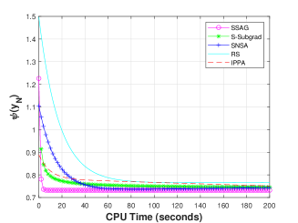
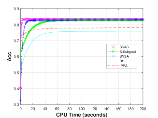
Figure 1: Average Obj and Acc v.s. CPU time of 20 runs on a8a, when $\tau=0.005$ and $\epsilon=0.001$.

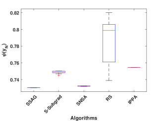
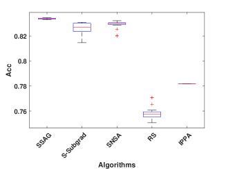
Figure 2: The boxplots of Obj and Acc of 20 runs on a8a, when $\tau=0.005$ and $\epsilon=0.001$.

Next, to compare the classification accuracy of these methods, cross-validation (CV) is used to select the best $\tau$ for each method. Apart from a8a dataset, we also test on 2-class versions of MnistData-10, and TDT2 datasets, denoted as MnistData-10(B), and TDT2(B), respectively. We adopt a similar approach to [23] by analyzing datasets in 2-class versions. MnistData-10 dataset is composed of handwritten digits, available from the website. MnistData-10(B) discriminates between the first 5 classes and the remaining ones. TDT2 dataset can be downloaded from the website. TDT2(B) discriminates between the first 15 classes and the remaining ones. The total number of samples $N_{\rm{tol}}$ and the dimension $d$ of each sample are listed in Table 3.

We choose the optimal value of parameter $\tau$ via the 3-fold CV using 20 random runs, which are determined by varying it on the grid $\{0;0.005\times l,l=1,\ldots,14\}$ and the values with the best average Acc are chosen for each of the SSAG, S-Subgrad, SNSA, RS, and IPPA methods. We use the predetermined accuracy $\epsilon=0.001$. We record in Table 3 the parameter $\tau$ we find by the 3-fold CV, together with the corresponding average Acc of the computed solution and the average CPU time to find the computed solution in seconds. We can see that our SSAG method has the best average accuracy for all datasets. The CPU times of the SSAG method are faster than those of the other methods.

Table 3: Acc and CPU time determined by 3-fold CV on three datasets with parameters $(\overline{N},\tau,\mu,m)$

Dataset ($N_{\rm{tol}},d$)	$\overline{N}$	ALG.	$\tau$	$\mu$	$m$	Acc	CPU
a8a (22696,123)	4.39e+08	SSAG	0.000	$\downarrow$	2000	0.8362	23.60
		S-Subgrad	0.020	-	2000	0.8003	200.00
		SNSA	0.000	6.16e-04	15058	0.8139	136.37
		RS	0.000	$\downarrow$	10000	0.7623	200.00
		IPPA	0.015	-	15130	0.8005	200.00
MnistData-10(B) (6996,784)	1.13e+09	SSAG	0.060	$\downarrow$	1000	0.8586	42.22
		S-Subgrad	0.045	-	1000	0.8158	200.00
		SNSA	0.050	1.88e-04	16795	0.8426	200.00
		RS	0.050	$\downarrow$	1000	0.7978	200.00
		IPPA	0.060	-	4664	0.8387	200.00
TDT2(B) (9394,36771)	1.18e+12	SSAG	0.060	$\downarrow$	3000	0.9906	47.08
		S-Subgrad	0.040	-	3000	0.9425	200.00
		SNSA	0.065	1.56e-04	29518	0.9626	198.74
		RS	0.060	$\downarrow$	30000	0.8781	200.00
		IPPA	0.060	-	6262	0.9573	200.00

4.2 DRPO

Risk management in portfolio optimization determines an optimal weight for each asset, by solving specific optimization problems reflecting the risk attitudes of the manager on known data samples [18, 22]. We consider the following distributionally robust portfolio optimization problem (Example 5.1 of [38]):

(58) $$\min\limits_{x\in\Delta_{d}}\max\limits_{P\in\mathcal{P}}\mathbb{E}_{P}[-\langle\zeta,x\rangle].$$

where $\zeta_{j}$ is the random return rate of asset $j$, and $x_{j}$ is the proportion of asset $j$ among all assets, $j=1,\ldots,d$. The ambiguity set $\mathcal{P}$ is described by moment constraints that rely on estimates of the mean $\hat{\mu}_{0}$ and covariance matrix $\hat{\Sigma}_{0}$ of the random vector; see Example 2.3 of [38] for detail. To be specific,

(59) $$\mathcal{P}:=\left\{\begin{aligned} &\mathbb{E}_{P}\left[\hat{\mathbf{\phi}}_{1}\left(\zeta\right)\right]\preceq 0\\ P\in\mathscr{P}\left({\Xi_{\zeta}}\right):~{}&\mathbb{E}_{P}\left[\hat{\mathbf{\phi}}_{2}\left(\zeta\right)\right]\preceq 0\\ &\mathbb{E}_{P}\left[1\right]=1\end{aligned}\right\},$$

where $\mathscr{P}\left({\Xi_{\zeta}}\right)$ denotes the set of all probability distributions over the support set ${\Xi_{\zeta}}$,

$$\hat{\mathbf{\phi}}_{1}\left(\zeta\right)=\left(\begin{array}[]{cc}-\hat{\Sigma}_{0}&\hat{\mu}_{0}-\zeta\\ \left(\hat{\mu}_{0}-\zeta\right)^{T}&-\gamma_{1}\end{array}\right),$$

$\hat{\mathbf{\phi}}_{2}\left(\zeta\right)=\left(\zeta-\hat{\mu}_{0}\right)\left(\zeta-\hat{\mu}_{0}\right)^{T}-\gamma_{2}\hat{\Sigma}_{0}$, $\gamma_{1}=0.1$, and $\gamma_{2}=1.1$. The mean and covariance matrix $\hat{\mu}_{0}$ and $\hat{\Sigma}_{0}$ are calculated through samples obtained from historical data.

Let $\mathbf{x_{\Lambda}}:=(x,\Lambda_{1},\Lambda_{2})$. As in [38], through Lagrange dual and discretization, (58) can be approximately solved by

(60) $$\min\limits_{x,\Lambda_{1},\Lambda_{2}}{} \max\limits_{\xi\in\ \{1,\ldots,q\}}\left\{h_{\xi}(\mathbf{x_{\Lambda}}):=-\langle\zeta^{\xi},x\rangle-\sum\limits_{i=1}^{2}\left\langle\Lambda_{i},\hat{\mathbf{\phi}}_{i}\left(\zeta^{\xi}\right)\right\rangle\right\}$$

s.t. $$x\in\Delta_{d},$$

$$\Lambda_{i}\succeq 0,\text{ for }i=1,2,$$

where $\zeta^{1},\ldots,\zeta^{q}$ are independent and identically distributed samples in $\Xi_{\zeta}$. We employ the smoothing function (20) and obtain the smoothing problem of (60) as

(61) $$\min\limits_{x,\Lambda_{1},\Lambda_{2}} \mu\ln\left(\sum\limits_{\xi=1}^{q}e^{\frac{h_{\xi}(\mathbf{x_{\Lambda}})}{\mu}}\right)$$

s.t. $$x\in\Delta_{d},$$

$$\Lambda_{i}\succeq 0,\text{ for }i=1,2.$$

We use a historical daily return rate of $d=40,80$ stocks between January 2005 and July 2023 from National Association of Securities Deal Automated Quotations (NASDAQ) index, which contains $N_{\rm{tol}}=4675$ samples. We denote the daily return rates of $d$ assets on the $j$-th day as $\zeta^{j}=(\zeta^{j}_{1},\zeta^{j}_{2},\ldots,\zeta^{j}_{d})^{\top}$, where $\zeta^{j}_{i}$ represents the ratio of the closing price to the opening price of the $i$-th asset on the $j$-th day for $j=1,\ldots,N_{\rm{tol}}$.

Three methods are employed to solve (60), and each method runs 20 times. We list the mean of objective value (Obj) in the training set, and the CPU time in Table 4. Since Subgrad and CP are deterministic methods, the objective values of 20 times are the same, which leads “Obj Var” to be 0. It is clear that SSAG provides the computed solutions with the smallest “Obj Mean” for $\epsilon=0.01,~{}0.001,~{}0.0001$ among all the methods. The “Obj Var” is also very small. Moreover, we can see from the last column of Table 4 that the proposed SSAG method can obtain the desired objective value within 20 seconds, and the CPU time does not grow dramatically as the dimension $d$ increases, and the $\epsilon$ decreases. In contrast, the CPU time of the Subgrad method grows quickly as $\epsilon$ decreases. The CP method, however, can not obtain the desired value within the time budget 200s for all the cases.

Table 4: Obj and CPU time with parameters $(d,\epsilon,\overline{N},\mu,m)$

$d$	$\epsilon$	$\overline{N}$	ALG.	$\mu$	$m$	Obj	Obj	CPU
						Mean	Var
$40$	0.01	2.04e+06	SSAG	$\downarrow$	100	-0.7045	1.17e-07	8.22
			Subgrad	-	4675	-0.6944	0	33.82
			CP	-	4675	5.8572	0	200.00
	0.001	2.20e+07	SSAG	$\downarrow$	100	-0.7159	8.49e-08	10.71
			Subgrad	-	4675	-0.7150	0	104.53
			CP	-	4675	5.8572	0	200.00
	0.0001	3.87e+08	SSAG	$\downarrow$	100	-0.7235	1.06e-07	11.88
			Subgrad	-	4675	-0.7228	0	200.00
			CP	-	4675	5.8572	0	200.00
$80$	0.01	2.03e+06	SSAG	$\downarrow$	100	-0.1347	3.68e-08	6.78
			Subgrad	-	4675	-0.1334	0	39.68
			CP	-	4675	31.9135	0	200.00
	0.001	2.12e+07	SSAG	$\downarrow$	100	-0.1083	2.79e-08	11.96
			Subgrad	-	4675	-0.1075	0	128.21
			CP	-	4675	31.9135	0	200.00
	0.0001	2.92e+08	SSAG	$\downarrow$	100	-0.1106	4.10e-08	17.92
			Subgrad	-	4675	-0.1098	0	200.00
			CP	-	4675	31.9135	0	200.00

Fig. 3 draws the boxplots of Obj in the training data for all methods in 20 runs, when $\epsilon=0.001$. Due to the similarity, we omit the figures of $\epsilon=0.01$ and $\epsilon=0.0001$. It is clear that our SSAG method performs much better than the others.

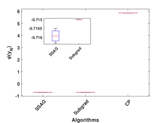
(a) $d=40$

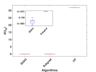
(b) $d=80$

Figure 3: The boxplots of Obj in 20 runs, when $\epsilon=0.001$.

We also employ the same stopping criteria used in [38] for the CP method, and then run the SSAG method and the Subgrad method using the same CPU time as that for the CP method to stop. We plot in Fig. 4 the average Obj v.s. CPU time when the stopping criteria in [38] is employed. The two small inner figures are the enlarged beginning period and ending period of the large figure, respectively. We can observe that the SSAG method has the fastest descending speed. The Subgrad method fails to further reduce the objective value in the ending period. Eventually, the CP method obtains the optimal value, but it uses a much longer CPU time than our SSAG method.

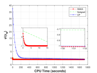
(a) $d=40$

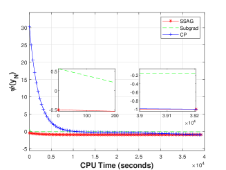
(b) $d=80$

Figure 4: Average Obj v.s. CPU time of 20 runs

5 Conclusions

In this paper, we propose a stochastic smoothing accelerated gradient method for solving nonsmooth convex composite minimization problems. Various smoothing techniques can be employed to construct smoothing functions (Definition 2.1) that also satisfy Assumption 2.1. We do not need the requirement that the nonsmooth component is of linear max structure as in [25, 35]. The requirement that the proximal operator of the nonsmooth component does not also need, compared to [7]. As far as we know, it is the first time to propose a stochastic smoothing accelerated first-order method to solve the constrained convex composite optimization problem whose nonsmooth term is the maximization of numerous nonlinear convex functions. The adaptive strategy for decreasing the smoothing parameter is also beneficial to faster computational speed. The complexity results match the best complexity results of the state-of-the-art SA methods using the first-order information. Moreover, the complexity results can be dimension-independent, unlike the complexity results of the RS method that are dimension-dependent. The effectiveness and efficiency of our SSAG method have been demonstrated by numerical results of distributionally robust optimization problems.

Acknowledgement. We are grateful to Prof. Yongchao Liu of Dalian University of Technology, for providing us the Matlab code of the CP method used in [38].

References

[1]Z. Allen-Zhu, Katyusha: The first direct acceleration of
stochastic gradient methods, J. Mach. Learn. Res., 18 (2017),
pp. 8194–8244.
[2]J. Bai, W. W. Hager, and H. Zhang, An inexact accelerated stochastic
ADMM for separable convex optimization, Comput. Optim. Appl., 81 (2022),
pp. 479–518.
[3]J. Bai, D. Han, H. Sun, and H. Zhang, Convergence on a symmetric
accelerated stochastic ADMM with larger stepsizes, CSIAM Trans. Appl.
Math., 3 (2022), pp. 448–479.
[4]H. H. Bauschke, Projection algorithms and monotone operators, PhD
thesis, Simon Fraser University, 1996.
[5]A. Beck, First-order Methods in Optimization, SIAM,
Philadelphia, 2017.
[6]A. Beck and M. Teboulle, Smoothing and first order methods: A
unified framework, SIAM J. Optim., 22 (2012), pp. 557–580.
[7]W. Bian and X. Chen, A smoothing proximal gradient algorithm for
nonsmooth convex regression with cardinality penalty, SIAM J. Numer. Anal.,
58 (2020), pp. 858–883.
[8]J. Cervantes, F. Garcia-Lamont, L. Rodríguez-Mazahua, and A. Lopez,
A comprehensive survey on support vector machine classification:
Applications, challenges and trends, Neurocomputing., 408 (2020),
pp. 189–215.
[9]O. Chapelle, V. Sindhwani, and S. S. Keerthi, Optimization
techniques for semi-supervised support vector machines., J. Mach. Learn.
Res., 9 (2008), pp. 203–233.
[10]C. Chen and O. L. Mangasarian, A class of smoothing functions for
nonlinear and mixed complementarity problems, Comput. Optim. Appl., 5
(1996), pp. 97–138.
[11]X. Chen, Smoothing methods for nonsmooth, nonconvex minimization,
Math. Program., 134 (2012), pp. 71–99.
[12]K. Crammer and Y. Singer, On the algorithmic implementation of
multiclass kernel-based vector machines, J. Mach. Learn. Res., 2 (2001),
pp. 265–292.
[13]A. Defazio, F. Bach, and S. Lacoste-Julien, SAGA: A fast
incremental gradient method with support for non-strongly convex composite
objectives, NIPS, 27 (2014), pp. 1646–1654.
[14]J. C. Duchi, P. L. Bartlett, and M. J. Wainwright, Randomized
smoothing for stochastic optimization, SIAM J. Optim., 22 (2012),
pp. 674–701.
[15]S. Ghadimi and G. Lan, Optimal stochastic approximation algorithms
for strongly convex stochastic composite optimization I: A generic
algorithmic framework, SIAM J. Optim., 22 (2012), pp. 1469–1492.
[16]S. Ghadimi and G. Lan, Accelerated gradient methods for nonconvex
nonlinear and stochastic programming, Math. Program., 156 (2016),
pp. 59–99.
[17]S. Ghadimi, G. Lan, and H. Zhang, Mini-batch stochastic
approximation methods for nonconvex stochastic composite optimization, Math.
Program., 155 (2016), pp. 267–305.
[18]P. J. Kremer, S. Lee, M. Bogdan, and S. Paterlini, Sparse portfolio
selection via the sorted -norm, J. Bank. Financ., 110 (2020),
pp. 105687.1–205687.15.
[19]G. Lan, An optimal method for stochastic composite optimization,
Math. Program., 133 (2012), pp. 365–397.
[20]G. Lan, S. Lee, and Y. Zhou, Communication-efficient algorithms for
decentralized and stochastic optimization, Math. Program., 180 (2020),
pp. 237–284.
[21]J. Li, C. Chen, and A. M.-C. So, Fast epigraphical projection-based
incremental algorithms for Wasserstein distributionally robust support
vector machine, NIPS, 33 (2020), pp. 4029–4039.
[22]L. Martínez-Nieto, F. Fernández-Navarro, M. Carbonero-Ruz, and
T. Montero-Romero, An experimental study on diversification in
portfolio optimization, Expert. Syst. Appl., 181 (2021),
pp. 115203.1–115203.14.
[23]S. Melacci and M. Belkin, Laplacian support vector machines trained
in the primal, Journal of Machine Learning Research, 12 (2011),
pp. 1149–1184.
[24]A. Nemirovski, A. Juditsky, G. Lan, and A. Shapiro, Robust
stochastic approximation approach to stochastic programming, SIAM J. Optim.,
19 (2009), pp. 1574–1609.
[25]Y. Nesterov, Smooth minimization of non-smooth functions, Math.
Program., 103 (2005), pp. 127–152.
[26]L. M. Nguyen, J. Liu, K. Scheinberg, and M. Takáč, SARAH: A novel method for machine learning problems using stochastic
recursive gradient, ICML, (2017), pp. 2613–2621.
[27]B. T. Polyak, New stochastic approximation type procedures,
Automat. i Telemekh., 7 (1990), pp. 98–107.
[28]B. T. Polyak and A. B. Juditsky, Acceleration of stochastic
approximation by averaging, SIAM J. Control Optim., 30 (1992), pp. 838–855.
[29]S. J. Reddi, A. Hefny, S. Sra, B. Póczos, and A. Smola, Stochastic variance reduction for nonconvex optimization, ICML, (2016),
pp. 314–323.
[30]H. Robbins and S. Monro, A stochastic approximation method, Ann.
Math. Statist., (1951), pp. 400–407.
[31]A. Ruszczyński and A. Shapiro, Stochastic Programming
Models, Elsevier, Amsterdam, 2003.
[32]P. K. Shivaswamy and T. Jebara, Relative margin machines., NIPS, 19
(2008), pp. 1481–1488.
[33]M. Singla, D. Ghosh, and K. Shukla, A survey of robust optimization
based machine learning with special reference to support vector machines,
Int. J. Mach. Learn. Cyb., 11 (2020), pp. 1359–1385.
[35]R. Wang, C. Zhang, L. Wang, and Y. Shao, A stochastic Nesterov’s
smoothing accelerated method for general nonsmooth constrained stochastic
composite convex optimization, J. Sci. Comput., 93 (2022), pp. 1–35.
[36]X. Wang, S. Wang, and H. Zhang, Inexact proximal stochastic gradient
method for convex composite optimization, Comput. Optim. Appl., 68 (2017),
pp. 579–618.
[37]Z. Wang, Y.-H. Shao, L. Bai, C.-N. Li, L.-M. Liu, and N.-Y. Deng, Insensitive stochastic gradient twin support vector machines for large scale
problems, Inf. Sci., 462 (2018), pp. 114–131.
[38]H. Xu, Y. Liu, and H. Sun, Distributionally robust optimization with
matrix moment constraints: Lagrange duality and cutting plane methods,
Math. Program., 169 (2018), pp. 489–529.
[39]M. Xu and J. J. Ye, A smoothing augmented Lagrangian method for
solving simple bilevel programs, Comput. Optim. Appl., 59 (2014),
pp. 353–377.
[40]M. Xu, J. J. Ye, and L. Zhang, Smoothing SQP methods for solving
degenerate nonsmooth constrained optimization problems with applications to
bilevel programs, SIAM J. Optim., 25 (2015), pp. 1388–1410.
[41]C. Zhang and X. Chen, Smoothing projected gradient method and its
application to stochastic linear complementarity problems, SIAM J. Optim.,
20 (2009), pp. 627–649.
[42]C. Zhang and X. Chen, A smoothing active set method for linearly
constrained non-Lipschitz nonconvex optimization, SIAM J. Optim., 30
(2020), pp. 1–30.
[43]K. Zhou, Y. Jin, Q. Ding, and J. Cheng, Amortized Nesterov’s
momentum: A robust momentum and its application to deep learning, UAI,
(2020), pp. 211–220.