Hyper-pixel-wise Contrastive Learning Augmented Segmentation Network for Old Landslide Detection through Fusing High-Resolution Remote Sensing Images and Digital Elevation Model Data

Abstract

As a natural disaster, landslide often brings tremendous losses to human lives, so it urgently demands reliable detection of landslide risks. When detecting old landslides that present important information for landslide risk warning, problems such as visual blur and small-sized dataset cause great challenges when using remote sensing data. To extract accurate semantic features, a hyper-pixel-wise contrastive learning augmented segmentation network (HPCL-Net) is proposed, which augments the local salient feature extraction from boundaries of landslides through HPCL-Net and fuses heterogeneous infromation in the semantic space from high-resolution remote sensing images and digital elevation model data. For full utilization of precious samples, a global hyper-pixel-wise sample pair queues-based contrastive learning method is developed, which includes the construction of global queues that store hyper-pixel-wise samples and the updating scheme of a momentum encoder, reliably enhancing the extraction ability of semantic features. The proposed HPCL-Net is evaluated on the Loess Plateau old landslide dataset and experimental results verify that the proposed HPCL-Net greatly outperforms existing models, where the mIoU is increased from 0.620 to 0.651, the Landslide IoU is improved from 0.334 to 0.394 and the F1score is enhanced from 0.501 to 0.565.

I Introduction

A landslide is a type of geological disasters with severe hazards, often resulting in traffic disruption, village burial, river blockage and other catastrophic incidents, threatening human life and property safety. For example, there have been 24 large-scale catastrophic landslides in Lanzhou City, China, since 1949, resulting in a total of 670 deaths and a direct economic loss of 776 million RMB [1]. Therefore, accurate and efficient prediction of landslides is of great significance for preventing or at least reducing such disastrous losses. Because existing landslides can provide useful information to aid prediction of potential landslides whose features have not yet fully formed presenting the greatest danger, and they could threaten to recur, we concentrate on the research of the existing landslide prediction.

Traditional existing landslide detection methods are mainly based on field investigation and remote sensing data, which can reliably recognize landslides but heavily rely on the experience of geological experts. Moreover, they are time-consuming and inefficient, making this approach difficult for being widely applied. With the rapid development of remote sensing technology, abundant ground-observable remote sensing data has been widely used in landslide detection. For example, Interferometric Synthetic Aperture Radar (InSAR) data can provide deformation characteristics of landslides [2], High-Resolution Satellite Image (HRSI) data can provide optical characteristics of landslides [3], Digital Elevation Model (DEM) data and Digital Surface Model (DSM) data can provide topographic characteristics of landslides [4, 5].

Automatic landslide detection using HRSI data can be regarded as one type of image processing tasks, and there are two classic methods based on HRSI, i.e., pixel-based classification method and object-oriented analysis (OBA) method. The first method classifies pixels based solely on spectral characteristics of the input image [6, 7, 8], which lacks the ability to identify spatially continuous regions. Also, salt-and-pepper noise is difficult to tackle by this method [9, 10]. The second method attempts to group adjacent pixels into segments or objects by a homogeneity factor, and further analyzes these segments or objects based on their spatial, texture, context, geometry, and spectral characteristics [11, 12, 13, 14, 15]. The OBA methods effectively reduce the number of the false positive samples that are missed by pixel-based methods. However, there are many segmentation thresholds such as relief and slope that need to be manually adjusted in OBA methods, which severely limits the widespread applications of these methods. As machine learning technology develops rapidly, some methods based on the support vector machine, random forest, and logistic regression have been proposed [16, 17, 18]. Furthermore, as a state-of-the-art image processing method, the convolutional neural networks (CNNs) are widely applied in the field of landslide image classification, object detection, semantic segmentation and other tasks due to their excellent end-to-end self-learning ablility and abstract representation capability. In [19] a landslide detection method based on the CNN and a regional growth algorithm is proposed to discriminate the region, boundary and center of landslides. In [20] a Siamese CNN based on dual-temporal landslide HRSI data is developed for the pixel-wise change detection of landslides and a generative adversarial network is introduced to suppress differences between two images in the time domain. In [21], a 3D spatial and channel attention module is designed to enhance the extraction of landslide features.

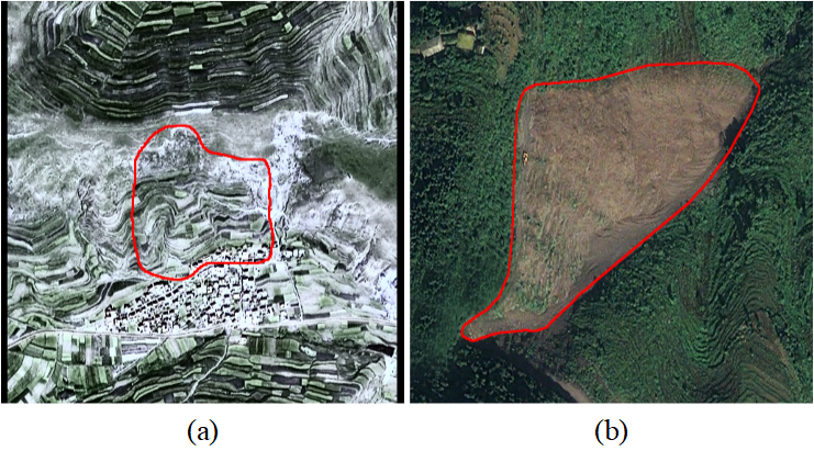
Figure 1: An example to show the visual differences between an old landslide and a new landslide. (a) old landslide; (b) new landslide.

However, existing works focus most on the identification of new landslides [19, 20, 21, 22, 23, 24, 25] rather than old landslides [26, 27]. Since landslides are formed by overall sliding of unstable structures in a slope along a shear plane under the influence of gravity [1], over time, landslide morphology gradually changes leading to a significant difference in morphology between new and old landslides. New landslides are in a state of repeated or just stopped activity, presenting visually obvious features, such as colors and contours distinct from the background. However, old landslides have been inactive for a long time, being severely affected by vegetation coverage, natural erosion, and human activities such as terracing, building houses, and constructing roads, as shown in Fig. 1. As a result, visual features of old landslides are blurry and difficult to distinguish from the background in optical images. Therefore, it is much easier to identify new landslides than old landslides. In addition, the detection of old landslide faces the small-sized dataset problem, because hidden visual features of old landslides make it difficult and time-consuming to label them, resulting in limited available data for the semantic segmentation of old landslides. Consequently, it is still an open problem for reliable detection of visually indistinct old landslides [27].

A reasonable approach for the challenge is to fuse heterogeneous semantic features from multi-modal data to provide richer information. In this paper, based on the expert knowledge that gradient patterns of landslides are significant for the recognition of landslides, we introduce DEM data to supply elevation features, and to fuse the two heterogeneous features extracted from HRSIs and DEM with the objective of improving the reliability of old landslide deteciton.

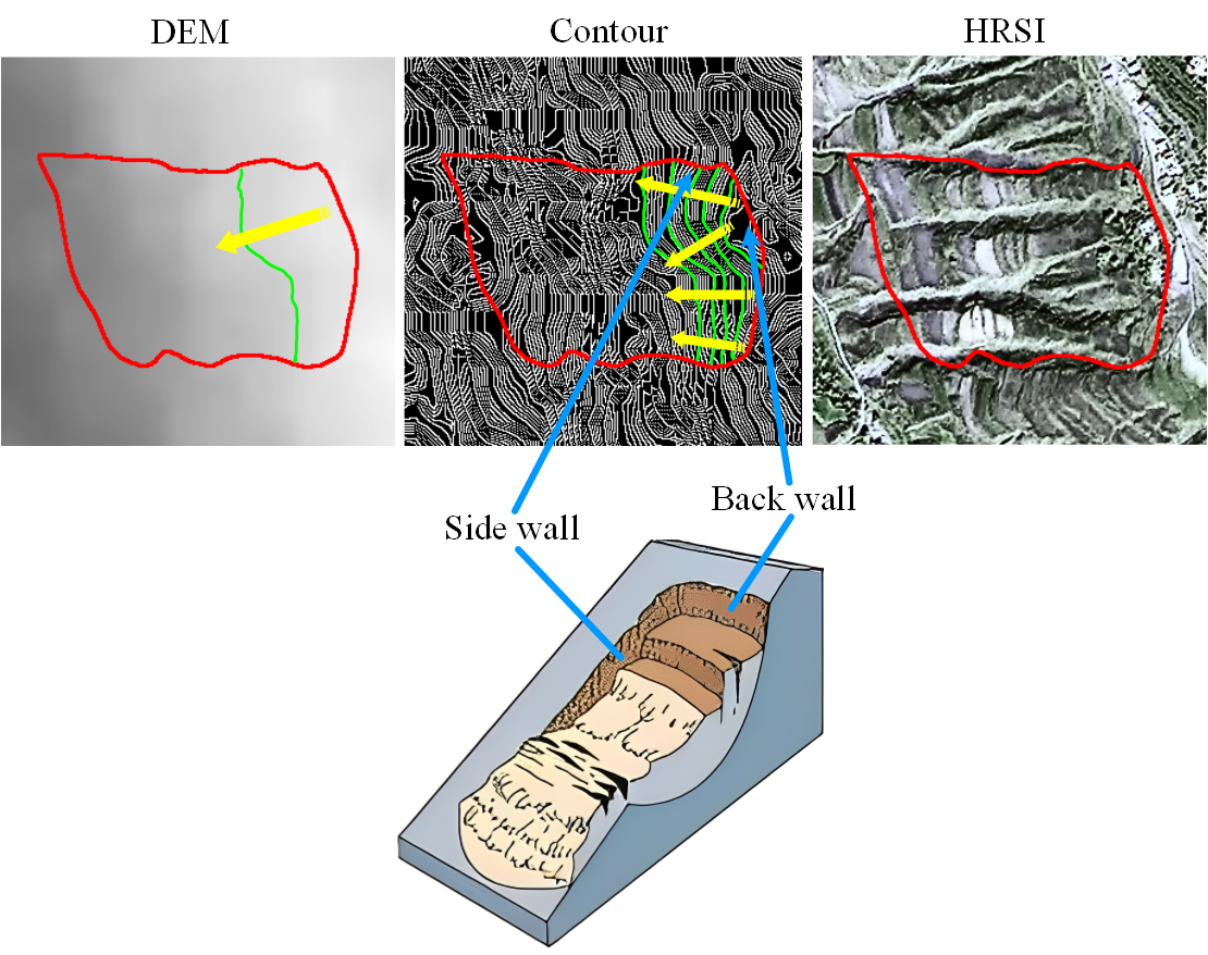
Figure 2: Illustration of projections from a 3D landslide (bottom) into DEM (left), Countour (middle) and HRSI (right). One of the salient features of a landslide is the steep altitude descent of back and side walls, which is located in light gray areas with high elevation in DEM. The contour map is obtained by applying the Gauss-Laplace edge operator to DEM, where the back wall is parallel to the contour lines, while the side wall is vertical to the contour lines highlighted in green. The yellow arrows indicate landslide aspect. The gradient variation features in DEM are projected as the texture features in HRSI. The bottom schematic diagram of landslide is taken from [28].

In order to tackle the small-sized dataset problem, we employ contrastive learning, which has shown excellent performance in self-supervised representation learning, to enhence the feature extraction ability. Based on the expert knowledge that the boundary features of back and side walls reflect the most elevation change of landslides as illustrated in Fig. 2, we propose a supervised hyper-pixel-wise contrastive learning method to force the model to learn these local salient features in the feature space with great efficiency and reliability. Herein, a hyper-pixel is an area of the original image related to a pixel in the high-level feature map in terms of position information. Moreover, a hyper-pixel contains much rich and abundant semantic information of a local region than a pixel in pixel-wise contrastive learning. In general, our main contributions are summarized in the following:

• We propose the HPCL-Net model for old landslide detection task to address the visual blur problem. Through designing a dual-branch heterogeneous feature extractor with the Coordinate Attention mechanism, optical features such as texture and color in HRSIs and crucial topographic features such as altitude and gradient in DEM data are extracted and effectively fused. Results of ablation experiments and Visualization analysis in hot maps validate the effectiveness of our proposed model.

• We propose a supervised hyper-pixel-wise contrastive learning method to tackle the small-sized dataset problem. Under the guidance of experts knowledge in the landslide recognition, hyper-pixel-wise sample pairs are constructed from the areas of the back walls and side walls of a landslide to enhance the local salient feature extraction ability of the model. To significantly improve the effectiveness of HPCL, we build a global category queues achiving cross-image contrast between anchors and keys in contrastive learning, and update the keys by momentum encoder to avoid the asynchronous update problem.

• Extensive experiments are conducted to evaluate the proposed model on a real old landslide dataset, and the experimental results demonstrate that HPCL-Net achieves a significant improvement in the reliability of detecting old landslides.

II Related Work

Multi-modal data fusion schemes can be roughly categorized into early fusion schemes [22, 21] and late fusion ones [5, 29, 30, 31]. The early fusion schemes integrate multi-modal data into multi-channel data, which can be easily implemented, such as regarding DEM as an addtional channel of HRSI in [22], and mixing satellite optical images, shape files of landslides’ boundaries and DEM data into one dataset in [21]. However, due to the fact that different modes of data often have different semantic and syntactic features (e.g., visual features such as morphology, texture, color can be extracted from HRSIs, and terrain features like height variation can be extracted from DEM), the data space after fusion is always complex and irregular, thus making further feature extraction from it quite challenging. This calls for more powerful models which place higher demands on datasets. The late-fusion methods, however, independently extract features and then fuse them in the semantic space, effectively fusing the essential semantic information required for the task from heterogeneous features. For example, in [5], the semantic features from near infrared, red, green (IRRG) spectrum and Digital Surface Model (DSM) data are concatenated in the channel dimension; in [29], optical image features and DSM data features are contenated; in [30], two regional feature maps from optical image and Synthetic Aperture Radar data are contenated; in [31], the features from HRSI and DEM data are fused by adding pixels with the same positions in spatial dimension.

Therefore, considering the heterogeneity between HRSIs and DEM data, we adopt the late-fusion method, where features are generally fused by pixel-wise addtion [31] and channel concat [5, 29, 30]. The pixel-wise addtion increases less complexity than the channel concat at the expense of the discriminative ability of the model to heterogeneous features, while the channel concat performs better when there are significant semantic differences between heterogeneous features, such as HRSI and DEM. In addtion, we argue that the simple pixel-wise addition performs well in [31] because the very limited number of samples cannot support high-capacity encoder. However, when data is fully utilized in a more efficient way, a more powerful encoder is expected to enhance the feature extraction performance. Therefore, on the basis of the designed contrastive learning scheme that enables a much stronger feature extraction ability on small-sized datasets, we upgrade the encoder in [31] through channel concatenation and the Coordinate Attention (CA) mechanism [32] when fusing heterogeneous features, so that the contrastive learning and improved encoder can bring the best in each other for efficient and reliable semantic feature extraction.

Contrasive learning does well in feature extraction, with the core idea that given an anchor, positive samples to the anchor are distinguished from a set of negative samples in the projected feature space. Traditional contrastive learning is applied to self-supervised learning, where positive and negative samples are defined through pretext tasks to provide supervised signals for self-supervised training [33]. In the first paradigm of contrastive learning [33, 34], positive samples are defined as the input image in current batch or its augmented versions, while negative samples are selected from a memory bank, a storage of samples outside the model updated along every batch. Since samples in the memory bank are encoded by encoders with different parameters, the fist paradigm faces the asynchronous update problem. In the second paradigm [35], external storage is discarded, and sample pairs are constructed within each mini-batch for end-to-end training, addressing the asynchronous update problem. However, the mini-batch size for end-to-end training have to be as large as possible, such as 8192, requiring huge computing resources. In this paper, due to the constraints of small-sized dataset and resources, we carry out the first paradigm with supervised global category queues as external storage. To alleviate the asynchronous problem, we re-encode the anchors using a momentum encoder before enqueuing them, which prevents the model from learning the distribution features of the parameters rather than the landslide features.

Basically, the excellent feature representation ability of contrastive learning originates from the structured contrastive loss. Furthermore, contrastive learning has shown high flexibility, as it only requires an appropriate pretext task with reasonable positive and negative sample pairs. Therefore, some works introduce contrastive learning into supervised tasks by providing supervised signals through labels rather than pretext tasks. These works can be categorized into object-wise contrast [36, 37] and pixel-wise contrast [38, 39, 40]. For the former, images are treated as samples and tasks are generally classification. In the latter, pixels in images are treated as samples to achieve structured pixel embedding space and tasks are generally dense prediction such as semantic segmentation. However, the information contained by adjacent pixels for the pixel-wise contrastive learning is highly homogenous. The sample pairs constructed by these pixels make little contribution for improving performance. Therefore, in order to avoid the redundancy in semantic information in pixel-wise contrast and to efficiently distill crucial features of landslides, we propose the hyper-pixel-wise contrast. Furthermore, we choose the hyper-pixels that contain regional semantic information of the back walls and side walls as positive samples. In this case, the hyper-pixels contain all the information related to the local area of a landslide.

III HPCL-Net Model

Considering the visual blur and small-sized dataset problems, we propose the HPCL-Net model using HRSI and DEM data for reliable detection of old landslide through feature fusion in the semantic space and supervised contrastive learning. As shown in Fig. 3, the HPCL-Net has a classic encoder-decoder architecture, where the encoder extracts optical features from HRSIs and topographical features from DEM data seperately, and fuses them in the semantic space by the two-branched heterogeneous feature extractor. Then the multi-scale abstract feature extractor further extracts higher-level semantic features, from which the decoder classifies each pixel into landslide or background.

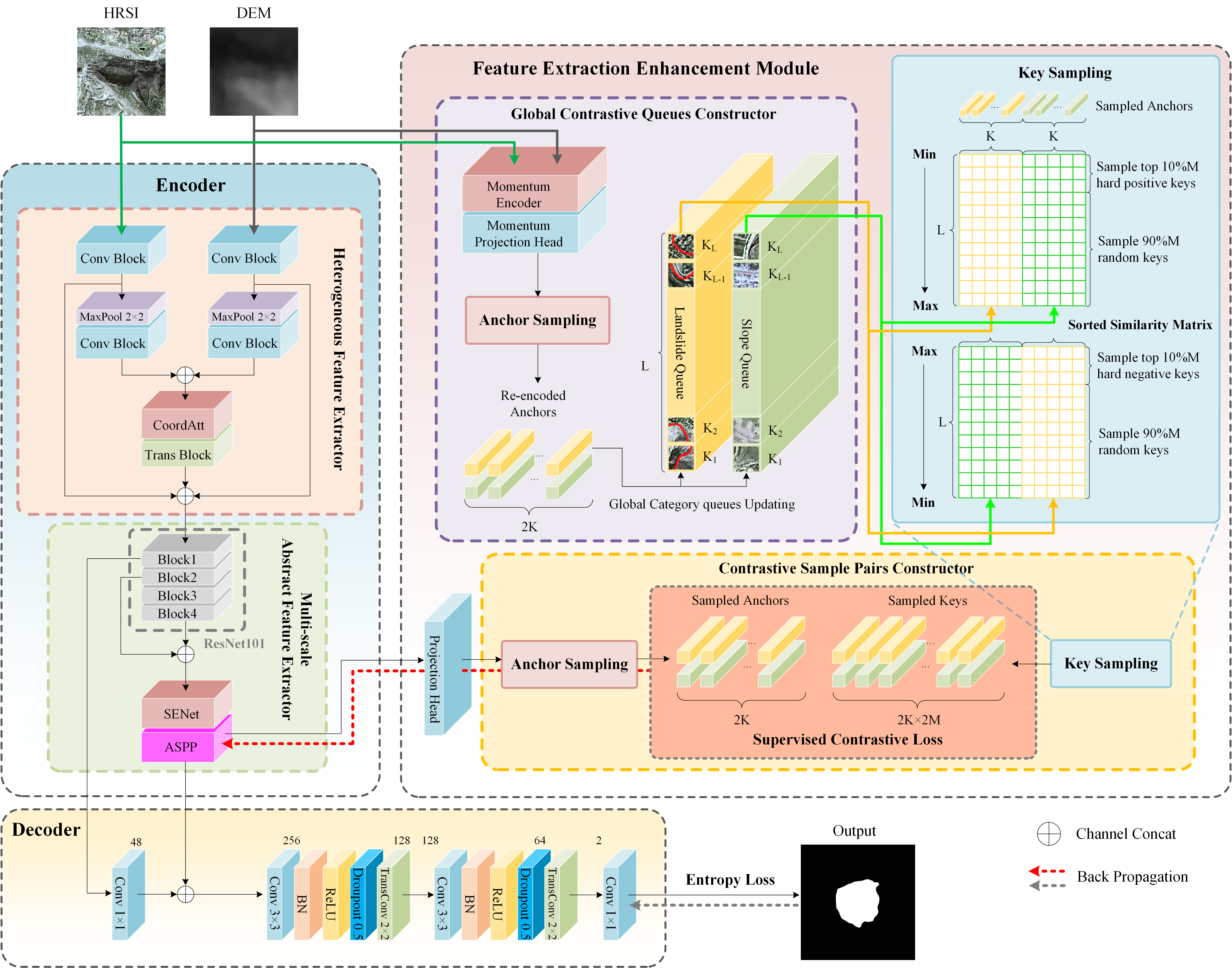
Figure 3: Architecture of HPCL-Net.

III-A Encoder

As shown in Fig. 3, the encoder consists of a Heterogeneous Feature Extractor and a Multi-scale Abstract Feature Extractor. Improved from our previous work [31], the newly designed encoder takes DEM data as an independent channel, and the heterogeneous features extracted independently from HRSIs and DEM data are fused through channel concatenation with the CA mechanism, contrasted to the scheme in [31] which duplicates the DEM data three times to facilitate the pixel addition with the RGB channel.

III-A1 Heterogeneous feature extractor

This module consists of a dual-branch network without weight-sharing and a feature fusion network whose architecture is detailed in Fig. 4. Each branch in the dual-branch network consists of a Conv Block, a max pooling layer, and a Conv Block sequentially, where the Conv Block includes a convolution layer, a batch normlization layer, and a ReLU layer. The HRSIs and DEM data are fed into the dual-brach network to first obtain two feature maps that are fused via channel concatenation and then weighted via the CA mechanism.

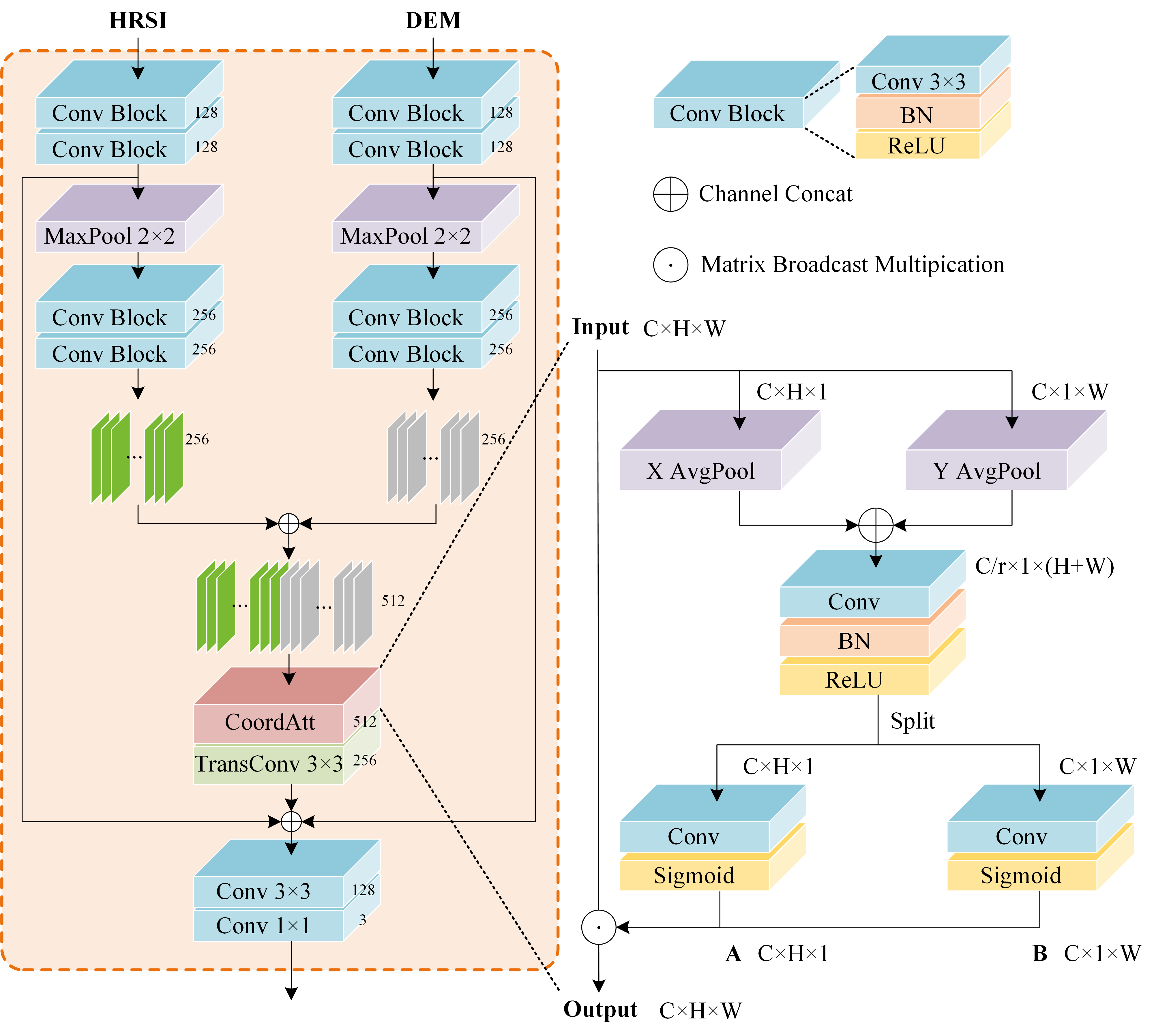
Figure 4: Architecture of the heterogeneous feature extractor. The sturcture of Coordinate Attention mechanism is indicated by the dotted line and the number on the right side of each component indicates the number of output channels.

As shown in Fig. 4, through the CA mechanism, two directional attention maps $A\in\mathbb{R}^{C\times H\times 1}$ and $B\in\mathbb{R}^{C\times 1\times W}$ are obtained, where $A$ represents $H$ attention wights for $Y$ direction, and $B$ represents $W$ attention wights for $X$ direction. Then, $A$ and $B$ weight the the original fused feature map of height $H$ and weight $W$ by matrix broadcast multiplication, i.e., expanding $A$ from $\mathbb{R}^{C\times H\times 1}$ to $\mathbb{R}^{C\times H\times H}$, and $B$ from $\mathbb{R}^{C\times 1\times W}$ to $\mathbb{R}^{C\times W\times W}$, then matrix-dot multiplying the original feature map and $A$, $B$. The CA mechanism integrates the cross-channel heterogeneous information and captures the direction and position-sensitive information as well, allowing the model to locate landslides more accurately. The weighted feature map is upsampled and concatenated with the feature maps produced by the first Conv Block, and the subsequent CNN extracts both high-level abstract semantic information and low-level spatial detailed syntactic information. In the heterogeneous feature extractor, batch normalization (BN) and ReLU are utilized after each layer to increase model stability and avoid overfitting.

III-A2 Multi-scale abstract feature extractor

In order to distinguish old landslides from backgrounds with high similarity, much higher abstract semantic features are required to extract from the fused features, which is implemented by the multi-scale abstract feature extractor. The backbone of the module is the dilated ResNet101 [41] that has been widely proven to have an excellent feature extraction capability. The ResNet101 consists of four dilated residual blocks. In order to retain more detailed features, the feature map of Block2 is concatenated with the upsampled feature map of Block4. The concatenated feature map is adaptively weighted through the SENet [42]. Then, the Atrous Spatial Pyramid Pooling [43] is used to effectively extract features at different scales through multiple parallel atrous convolution with different dilation rates. In addition, the global average pooling is used to gain global context information of the feature map.

III-B Feature Extraction Enhancement Module based on Supervised Hyper-pixel-wise Contrastive Learning

This module consists of two components, i.e., the Contrastive Sample Pairs Constructor (CSPC) and the Global Contrastive Queues Constructor (GCQC), where CSPC constructs hyper-pixel-wise positive and negative sample pairs, and GCQC enhances the efficiency and performance of contrastive learning. The architecture of the module is shown in Fig. 3.

Since the essential features of landslides are the gradient pattern, it is crucial to find the boundary areas of the back and side walls where the elevation is significantly decreased. For CSPC, under the anchor sampling strategy, the pixels from the high-dimensional feature map of the projection head are sampled as anchors. Each pixel corresponds to a hyper-pixel that is located at the boundary areas of the back walls/side walls or the background area. A hyper-pixel consists of a patch of pixels in the original image, which is illustrated in Fig. 5, and determined by label and DEM. Under the key sampling strategy, keys are selected from the queues to construct positive and negative sample pairs with anchors. Then, the supervised contrastive loss is calculated by the sample pairs. Through contrastive learning, the model can distill the essential differences between the semantic features of landslides and slopes. The word ‘supervised’ suggests that the class of each anchor and key is known from label.

Figure 5: Illustration of the hyper-pixel definition. Each $8\times 8$ blue square on HRSI, DEM or Label is a hyper-pixel corresponding to a pixel of 128 channels in the feature map produced by the projection head.

In CGQC, the global category queues contain a landslide queue and a slope queue that keep the keys outside the model. The queues are updated on-the-fly through enqueue and dequeue operations, where the enqueue operation denotes pulling the anchors re-encoded by the momentum encoder from the latest mini-batch into the queues, and the dequeue operation denotes pushing the keys from the oldest mini-batch out of the queues. Moreover, keys in the queues are selected from the entire dataset, which facilitates global contrastive learning for rich sample diversity.

III-B1 Contrastive sample pairs constructor

In this part, hyper-pixel-wise anchors and keys are sampled to build sample pairs and obtain the supervised contrastive loss.

a) Anchor sampling

In each batch, $K$ landslide anchors and $K$ slope anchors are sampled from the high-level feature map produced by the multi-scale abstract feature extractor of the encoder, and compared with the keys selected from the global category queues.

The sizes of the HRSI, DEM and label are $512\times 512$, and the high-level feature maps are reduced to $64\times 64$ through a series of convolution and down-sampling operations, where each pixel corresponds to a hyper-pixel that is an $8\times 8$ patch in the HRSI, DEM and label by location. If a hyper-pixel is located in the boundary area of back wall/side wall, the corresponding pixel is then sampled from the feature map as a candidate landslide anchor. The position of the candidate landslide hyper-pixel is determined in two steps as illustrated in Fig. 6, i.e., (1) The hyper-pixels with more than 6 and less than 58 landslide pixels are determined, which correspond to the boundary areas of the landslides; (2) Among these hyper-pixels, those with an average elevation greater than the median elevation of the entire landslide according to DEM are sampled candidate landslide anchors, meaning they are located on the back and side walls. The hyper-pixels without any landslide pixels within are sampled as candidate slope anchors.

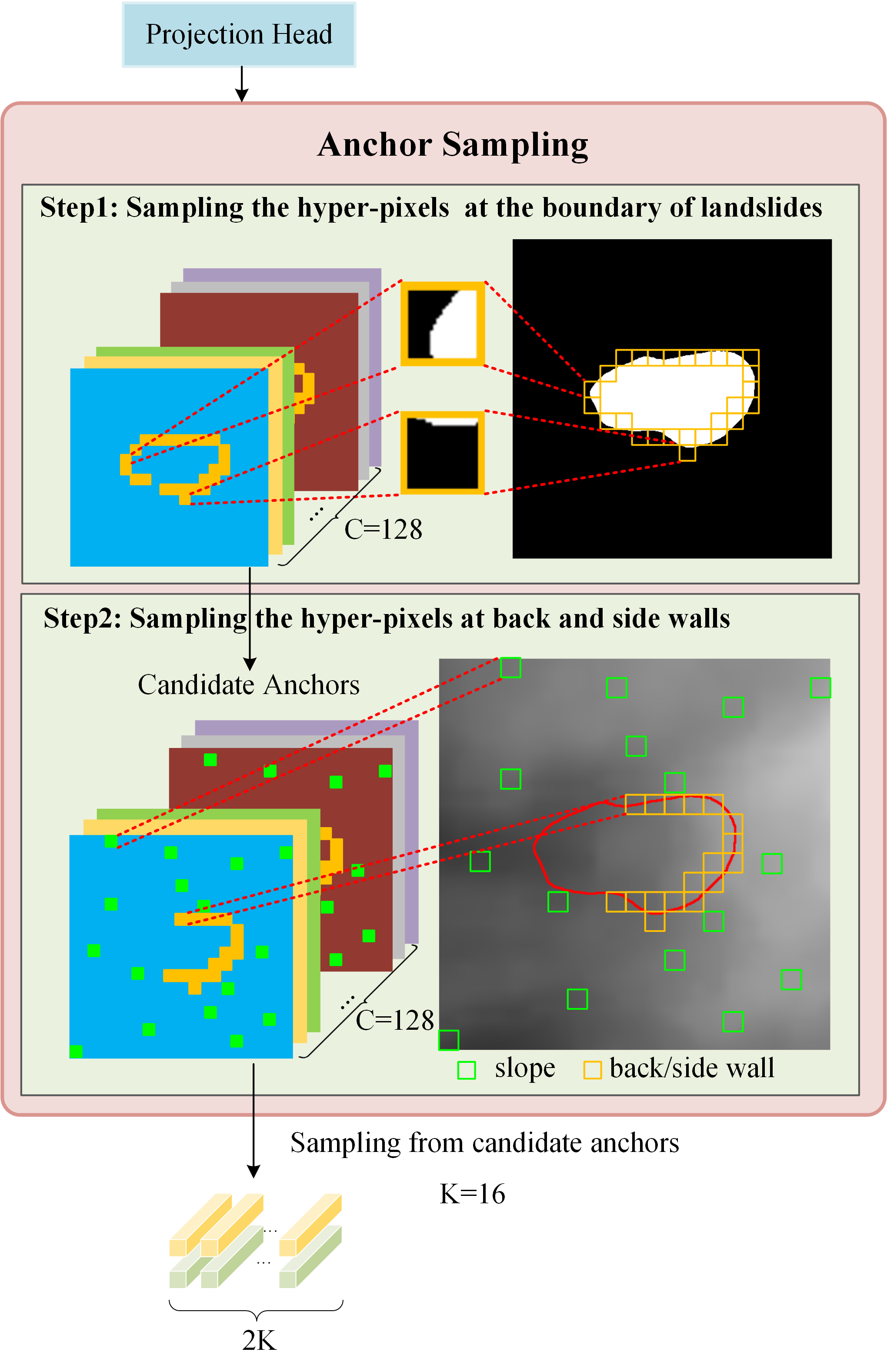
Figure 6: Anchor Sampling schematics. On the left of Steps 1 and 2 is the feature map produced by the projection head, from which anchors are sampled. Yellow boxes and squares mark sampled landslide hyper-pixels and anchors, while green boxes and squares mark sampled slope hyper-pixels and anchors. The correspondence between hyper-pixels and anchors is shown by the red dashed line.

The number of the channels in the high-level feature map from the encoder is 256 and then reduced to 128 through the projection head, so the anchor is a 128-dimensional vector. $K$ anchors are randomly sampled from the candidate anchors. We set $K$ to be 16.

b) Key sampling

For each of the aforementioned 2$K$ anchors, $M$ keys from the queue of the same category as the anchor are selected to construct the positive sample pairs with the anchor, another $M$ keys from the queue of the different category are selected to construct the negative sample pairs with the anchor.

In practice, the similarities between the anchor and all keys in queues are first calculated. In the queue of the same category, the top 10% $M$ keys with the lowest similarities are selected as the hard positive samples. Similarly, In the queue of the different category, the top 10% $M$ keys with the highest similarities are selected as the hard negative samples. The process of key sampling is illustrated in Fig. 3. These two types of hard samples can contribute more to the improvement of the discriminative ability [44, 45], and the remaining 90% $M$ keys are randomly sampled from the remaining keys in the queues, where $M$ is set to be 1000.

c) Supervised contrastive loss

The positive and negative sample pairs are used to calculate the supervised contrastive loss defined as follows

$$L_{i}^{SC}=\frac{1}{\left|P_{i}\right|}{\sum\limits_{i^{+}\in P_{i}}{-{\rm log}\frac{{\rm exp}\left(i\cdot i^{+}/\tau\right)}{{\rm exp}\left(i\cdot i^{+}/\tau\right)+{\sum_{i^{-}\in N_{i}}{{\rm exp}\left(i\cdot i^{-}/\tau\right)}}}}},$$ (1)

where $i$ denotes anchor $i$ sampled in the current batch, $P_{i}$ and $N_{i}$ denote the $M$ positive and negative samples, $i^{+}$ and $i^{-}$ denotes a key in $P_{i}$ and $N_{i}$ respectively, $\left|P_{i}\right|$ denotes the total number of $P_{i}$, i.e., $M$. $\tau$ is the temperature for controlling the shape of the distribution of logits that is in logarithmic scale. As $\tau$ decreases, the distribution of logits becomes more peak, enabling the model to focus on the hard samples. While as $\tau$ increases, the distribution of logits becomes smoother, reducing the sensitivity of the model to the difference between the anchors and keys. $\tau$ is set to 0.1 here. In addition, the larger $i\cdot i^{+}$ and the smaller $i\cdot i^{-}$, the smaller $L_{i}^{NCE}$ is. Therefore, by optimizing the loss, the distance between the anchors and positive keys will be closer and the distance between the anchors and negative keys will be farther.

III-B2 Global contrastive queues constructor

The specific configurations of the global category queues, momentum encoder and projection head are elaborated on below.

a) Global category queues

The gloabal category queues include the landslide and the slope queues of length $L$. Since keys are vectors of dimension $D$, the queue is a tensor of size $L\times D$. In addition, the queue adopts the first-in-last-out update strategy: $K$ new keys from latest mini-batch go into the queue, and $K$ old keys from the oldest mini-batch go out of the queue. Accordingly, $K$ is independent of $L$. By setting appropriate values of $K$ and $L$, substantial computing resources are saved and the training efficiency is thus improved. The queues are randomly initialized and a momentum encoder is used to re-encode anchors as new keys to update queues.

b) Momentum encoder and projection head

The momentum encoder [34] is introduced in GCQC to allows the new keys that are enqueued in different batches to be encoded by similar encoder parameters, avoiding the asynchronous update issue problem. The projection head [35] that consists of a simple $1\times 1$ convolutional layer is also introduced to reduce feature dimension for the improvement of training efficiency.

Practically, the momentum encoder and momentum projection head have the same architectures as the encoder and normal projection head, and are updated through momentum-based moving average showen below rather than back propagation. By feeding HRSIs and DEM data to both the encoder and momentum encoder, the pixels in the same positions as the anchors are sampled from the high dimensional feature map from the momentum projection head. These pixels are regarded as the re-encoded anchors, and then dimensionally reduced and pushed into the queues

$$\theta_{k}^{n}\leftarrow\left(\theta_{k}^{n-1}+\theta_{q}^{n}\right)\,,$$ (2)

$$P_{k}^{n}\leftarrow\left(P_{k}^{n-1}+P_{q}^{n}\right)\,,$$ (3)

where $\theta_{k}^{n}$, $\theta_{q}^{n}$, $P_{k}^{n}$, and $P_{q}^{n}$ denote the parameters of the encoder, the momentum encoder, the projection head, and the momentum projection head, respectively, from mini-batch $n$. $\theta_{k}^{n-1}$ and $P_{k}^{n-1}$ denote the parameters of the momentum encoder and the momentum projection head from mini-batch $n-1$, respectively, $m$ denotes momentum and is set to 0.999 here.

III-C Decoder

The feature map of Block1 in the ResNet101 concatenates with the output of the multi-scale abstract feature extractor in order to integrate low-level features such as details and spatial features with high-level abstract features, and then fed into the decoder.

The architecture of the decoder is shown in Fig. 3. The trainable filters of the transposed convolution reduce redundant information and have a better feature mapping capability to reconstruct the resolution of the input images.

The Cross-Entropy loss formulated below is used to calculate the loss between the category score map and the label where the landslide pixels are marked as 1 and others as 0.

$$L_{i}^{CE}=-y_{i}\left.{\mathit{\log}(}p_{i}\right)+\left(1-y_{i}\right)\left.{\mathit{\log}(}1-p_{i}\right),$$ (4)

where $y_{i}$ denotes the ground truth of pixel $i$ in the categoricy score map and $p_{i}$ indicates the probability of pixel $i$ being classified into landslide.

Therefore, the total training loss is

$$L={\sum_{i}}{\left(\alpha L_{i}^{CE}+\beta L_{i}^{C}\right)},$$ (5)

where $\alpha$ and $\beta$ are set to 1.0 and 0.1, respectively.

III-D Training Process

The overall training process of the HPCL-Net is given in the form of PyTorch-like pseudocode.

  Algorithm 1

 

  # f1, f2: Encoder and Momentum Encoder

  # p1: Projection Head

  # p2: Momentum Projection Head

  # m: momentum

  

  # Initialize

  f2.params = f1.params

  p2.params = p1.params

  

  # Load a mini-batch data

  for HRSI, DEM in loader:

    # Get encoder feature map

    map1 = f1(HRSI, DEM)

    # Get momentum encoder feature map

    map2 = f2(HRSI, DEM)

  

    # Sample anchors from the encoder feature map

    anchors = anchor_selection_strategy(map1)

    # Dimensional reduction by p1

    anchors = p1(anchors)

  

    # Re-encode anchors to new_keys

    new_keys = anchor_selection_strategy(map2)

    # Dimensional reduction by p2

    new_keys = p2(new_keys)

  

    # Update the queues

    enqueue(new_keys)

    dequeue(last_mini-batch_keys)

  

    # Sample keys from the queues

    keys = key_selection_strategy(queues)

  

    # Decoder output the categorical score map

    score_map = decoder(map1)

  

    # Loss

    loss1 = SCLoss(anchors, keys)

    loss2 = Cross_Entropy_Loss(secore_map, label)

    loss = $\alpha$loss1 + $\beta$loss2

  

    # Update momentum encoder and projection head

    f2.params = f2.params * m + f1.params * (1-m)

    p2.params = p2.params * m + p1.params * (1-m)

  

    # Backpropagation to update f1, p1 and decoder

    loss.backward()

    update(f1.params, p1.params, decoder.params)

 

IV Experiments

IV-A Experimental Setup

IV-A1 Dataset

The study area locates in the Loess Plateau of China, where the parent material of soil is residual and alluvial. Moreover, the soil there is generally sticky and has weak mitogenicity, permeability, corrosion resistance and erosion resistance, which are attributed to the occurrence of landslides in the past.

The Loess Plateau old landslide dataset contains 141 old landslide samples cropped to the size of $512\times 512$. The HRSIs are RGB images and the DEM data are grayscale images. Some samples are shown in Fig. 7. These images are divided into the training, validation, and test sets in a ratio of 6:2:2. The resolution of the HRSI is 2m/pixel, and the resolution of the DEM data is originally 30m/pixel and subsequently interpolated to match the resolution of the HRSI.

All the training and validation images are augmented by horizontal flipping, vertical flipping and rotating for $90^{\circ}$, $180^{\circ}$ and $270^{\circ}$. Histogram equalization is implemented as well.

IV-A2 Software and hardware environment

All experiments are conducted on a Linux server with the following configurations: Intel (R) Core (TM) i9-12900K@3.9 GHz, 16 cores, 128G RAM; NVIDIA 3090 24G; PyTorch Lightning 1.6.3.

IV-A3 Reference Model

We compare the HPCL-Net with the FFS-Net [31] that is considered as the baseline model. Since the FFS-Net has shown that it outperforms universal semantic segmentation models such as the UNet and Deeplabv3+ for landslide detection, we do not need to repeat the same comparison experiments. In addition, other multi-modal data fusion models [2, 5, 22, 21, 29, 30] use the data such as DSM, aerial photograph and InSAR greatly different from our HRSIs and DEM data, where DSM and aerial photograph have much higher resolution, and InSAR contains distinctive semantic features such as deformation rate. So, it is difficult to directly migrate the HRSIs and DEM data to these models. Besides, the tasks of these models are different from ours, e.g., the landslide classification [21] and image registration [30], and the source codes of these models have not been publicly released, so we cannot reproduce their results. Considering the above cases, we have to solely compare our model with the FFS-Net.

IV-A4 Hyperparameters

In all experiments, the stochastic gradient descent is chosen as the optimizer and the polynomial annealing policy [46] is used to schedule the learning rate. The hyperparameters and their values in this study are shown in Table I.

TABLE I: HYPERPARAMETERS.

Item	Value
Mini-batch Size	2 [t]
Epoch	100 [t]
Initial learning rate	0.007 [t]
Weight decay	0.007 [t]
Momentum	0.9 [t]
Optimizer	SGD [t]

IV-B Performance Metrics

The mainstream performance metrics such as $Precision$, $Recall$, $F1score$, $Landslide\_IoU$ and mean Intersection over Union ($mIoU$) are employed, which are defined as follows

$$precision=\frac{TP}{TP+FP}\,,$$ (6)

$$recall=\frac{TP}{TP+FN}\,,$$ (7)

$$F1score=2\times\frac{precision\times recall}{precision+recall}\,,$$ (8)

$$Landslide\underline{~{}}IoU=\frac{TP}{TP+FP+FN}\,,$$ (9)

$$Slope\underline{~{}}IoU=\frac{TN}{TN+FN+FP}\,,$$ (10)

$$mIoU=\frac{1}{2}\times(Landslide\underline{~{}}IoU+Slope\underline{~{}}IoU)\,,$$ (11)

where $TP$, $TN$, $FP$, $FN$ denote the numbers of correctly predicted landslide pixels, correctly predicted non-landslide pixels, incorrectly predicted landslide pixels, and incorrectly predicted non-landslide pixels, respectively.

IV-C Results and Discussions

In this section, we carry out comparison experiments, ablation experiments, and cross validation experiments, along with discussions on the experimental results.

IV-C1 Overall comparative experiments

The numeric results in Table II show that our proposed HPCL-Net performs better than the FFS-Net with $mIoU$ increased by 3.1%, $Landslide\_IoU$ increased by 6.0%, and $F1score$ increased by 6.4%, indicating reliable detection of old landslides. These improvements validate the effectiveness of the contributions in this paper.

TABLE II: Numerical results of segmentation networks

Method	Precision	Recall	F1	Landslide_IoU	mIoU
FFS-Net	0.462	0.551	0.501	0.334	0.620 [t]
HPCL-Net	0.579	0.573	0.565	0.394	0.651 [b]

The graphical segmentation results in Fig. 7 show that, compared to the FFS-Net, our results retain finer boundaries and are more accurate in shape and position, which are consistent with the numerical results.

Figure 7: Graphical segmentation results on the old landslides. From top to bottom are RGB, DEM, label, FFS-Net and ours.

To visualize the landslide features learned by each model, the Gradient-weighted Class Activation Mapping (Grad-CAM) scheme [47] is employed to produce a heatmap, where features with more contribution to the target class have higher heat. We apply Grad-CAM to the last layer of the encoders of the FFS-Net and HPCL-Net, and the heatmaps are shown in Fig. 8. Compared to the FFS-Net, our model has more features with higher heat located in the back and side walls of the landslides, proving that the proposed model is capable of effectively learning the crucial features of old landslides.

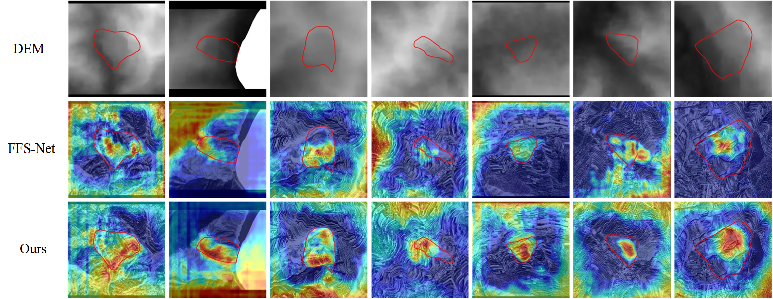
Figure 8: Visualization results for the last layer of the encoder by Grad-CAM. The landslides are outlined by the red line.

IV-C2 Ablation experiments

To precisely evaluate the contribution of each module in the proposed model, we conduct ablation experiments. The numerical results are shown in Table III, where FFS-Net is regarded as baseline; ‘B+F’ denotes employing newly designed heterogeneous feature extractor on the baseline; ‘B+F+C’ denotes a simplified end-to-end version of the HPCL-Net where the anchors and keys for contrastive learning are only sampled within the current mini-batch; ‘B+F+C+G’ denotes the final version of the HPCL-Net. The numerical ablation results show that:

• By improving the feature extraction and fusion module in the FFS-Net, the model performance is enhanced, where $mIoU$ is increased by 0.5%, $Landslide\_IoU$ is increased by 0.5%, and $F1score$ is increased by 0.5%. These enhancements show the effectiveness of the designed heterogeneous feature extractor.

• After adding CSPC, although $mIoU$ is slightly decreased, $Landslide\_IoU$, which is more essential for the task in practice, is increased by 1.2%, and the $F1score$ is also increased by 1.4% from the previous experiment. These enhancements demonstrate that the proposed CSPC makes certain contributions to the identification of landslide features. As for the reasons of no increase in $mIoU$, we argue that the end-to-end training paradigm is difficult to satisfy the necessary requirements for a large number of samples in contrastive learning. So we design GCQC to fix this problem.

• After applying GCQC to provide sufficient samples and improve sample diversity, the performance of the model is significantly improved, where $mIoU$ is increased by 2.7%, $Landslide\_IoU$ is increased by 4.3%, and $F1score$ is increased by 4.5%, proving our previous argument and the effectiveness of GCQC.

TABLE III: Numeric results of ablation experiments

Scheme	Precision	Recall	F1	Landslide_IoU	mIoU
B	0.462	0.551	0.501	0.334	0.620
B+F	0.449	0.589	0.506	0.339	0.625
B+F+C	0.545	0.520	0.520	0.351	0.624
B+F+C+G	0.579	0.573	0.565	0.394	0.651
B: Base model, i.e., FFS-Net
F: heterogeneous feature extractor
C: Contrastive sample pairs constructor
G: Global Contrastive Queues constructor

The graphical segmentation results of the four ablation experiments are shown in Fig. 9. The heterogeneous feature extractor can reduce misclassifications of the landslides, as highlighted by the red circles. After adding CSPC, the shape of the segmented landslide is more complete, and the position is more accurate, as highlighted by the blue circles. For the final model, the segmentation of the boundaries are the most clear and precise, which is consistent with the numerical results.

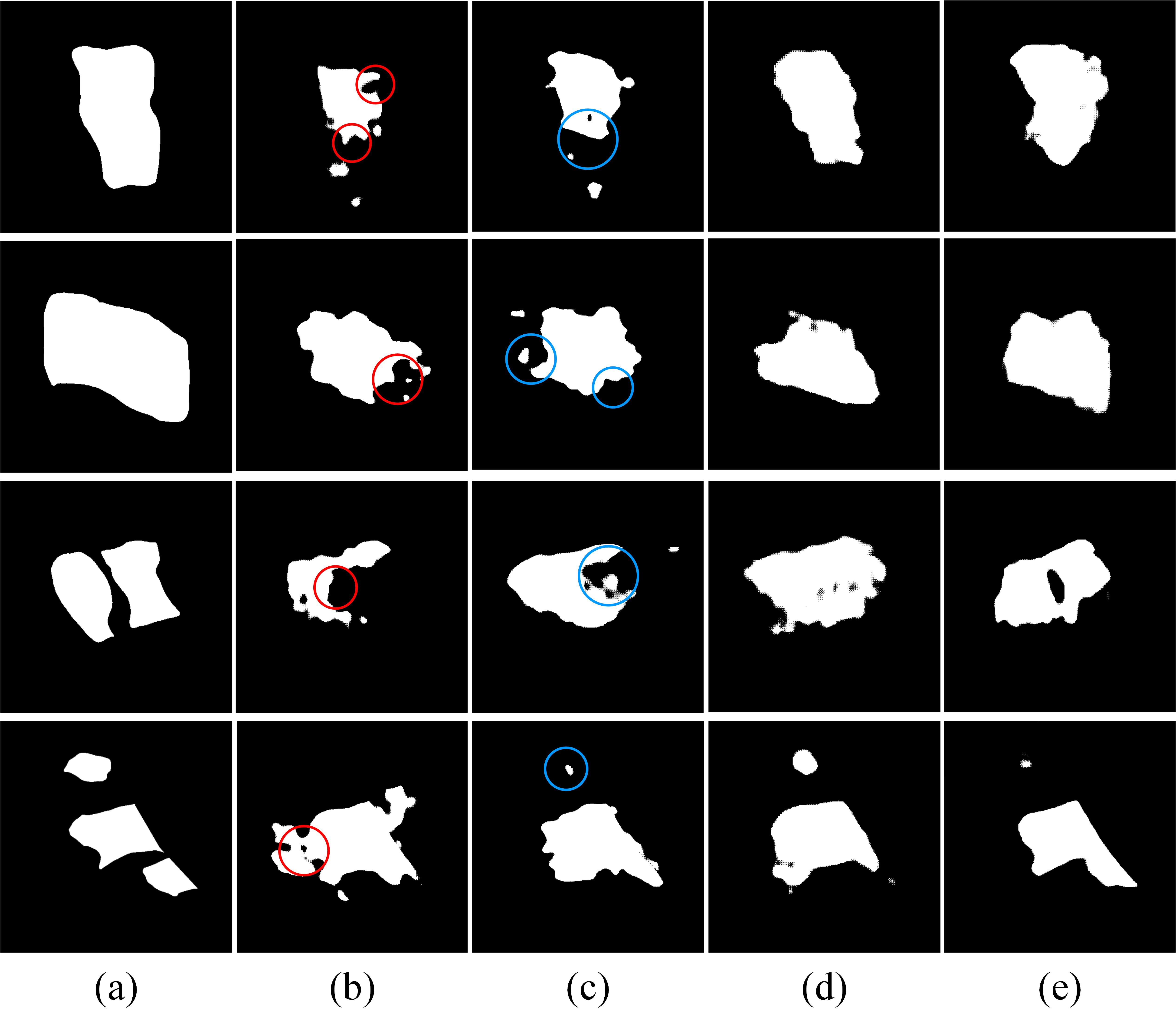
Figure 9: Visualization results for the encoder feature map. (a) label; (b)-(e): B; B+F; B+F+C; B+F+C+G.

To visualize the enhancements of the learned features corresponding to the increases of the performance metrics, we first choose the last layer of the feature extraction and fusion module in ‘B’ and the heterogeneous feature xtractor in ‘B+F’ as the target layer of the Grad-CAM. The heatmaps are shown in the Fig. 10, where the images in the last column are the contour maps obtained by applying the Gauss-Laplace edge operator to the DEM data. As can be seen from the figure, the heatmaps from ‘B’ have almost no visible optical or topographic features, while the heatmaps from ‘B+F’ have higher heat at the positions where elevation changes, forming the texture similar to the contour map. This indicates that by changing the fusion method to channel concatenation and introducing the CA mechanism, the designed heterogeneous feature extractor can effectively integrate the gradient features from the DEM data and color, texture, and other optical features from the HRSI.

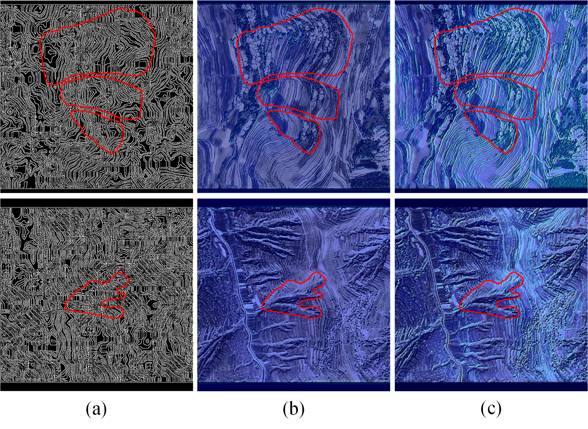
Figure 10: Visualization results for the last layer of the feature extraction and fusion module in FFS-Net and the heterogeneous feature extractor in HPCL-Net. The outline of the target landslide is highlighted in red line. (a) contour map; (b) B; (c) B+F.

Then, we choose the last layer in the encoders from the four experiments as the target layer of the Grad-CAM. Fig. 11 shows that the heatmaps generated by ‘B’ and ‘B+F’ have higher heat in the center of the landslide. However, after adding CSPC, the higher-heat areas in ‘B+F+C’ tend to the back wall and side wall areas of the landslide, demonstrating that the CSPC enables the model to focus on identifying essential features of landslides. In the heatmaps generated by ‘B+F+C+G’, the higher-heat areas are mostly concentrated on the back wall and side wall areas, suggesting that GCQC, which facilitates training with sufficient and diverse samples, plays a significant role in enbling the model to effectively learn crucial features.

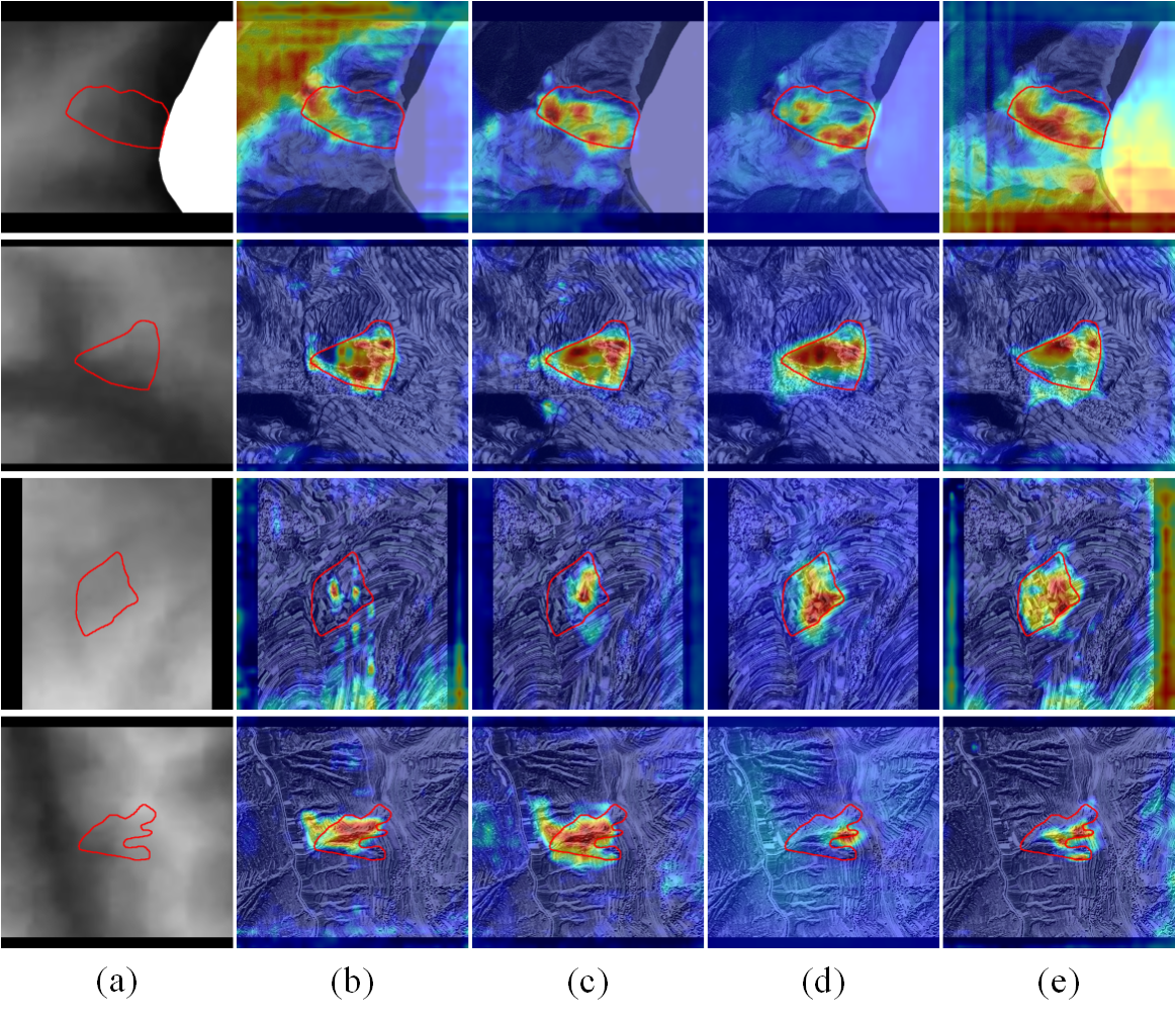
Figure 11: Visualization results for the last layer of encoder by Grad-CAM. The outlines of landslides are highlighted by red line. (a) label; (b)-(e): B; B+F; B+F+C; B+F+C+G.

IV-C3 Cross validation experiments

TABLE IV: Cross validation of fusion method

Experiment	Precision	Recall	F1	Landslide_IoU	mIoU
Baseline: CA + Channel Concat	0.462	0.551	0.501	0.334	0.620 [t]
CA + Pixel Addition	0.449	0.589	0.506	0.339	0.625 [t]
SENet + Channel Concat	0.545	0.520	0.520	0.351	0.624 [t]
CBAM + Channel Concat	0.579	0.573	0.565	0.394	0.651 [t]

In the section, we conduct cross-validation experiments for optimizing the model design. The baseline model is the HPCL-Net with the CA mechanism and the fusion method of channel concatenation. We first replace the channel concatenation with pixel addition. Then we replace the CA mechanism with the SENet and CBAM in the following experiments to compare the CA mechanism with the other two attention mechanisms.

The numerical results of the experiments are listed in Table IV. The result of replacing channel addition demonstrates that the channel concatenation method is more appropriate than pixel addition to fuse the features with a significant semantic difference from HRSI and DEM, which is consistent with the previous analysis. The results of relacing the CA mechanism show that the CA mechanism enables the model to fuse features from both the channel and spatial dimensions and performs better than the SENet that focuses on only channel attention. Compared with CBAM that also focuses on channel and spatial attention, although $mIoU$ is almost the same, $F1score$ of the HPCL-Net is 1.6% higher than the model with CBAM, proving the superiority of the CA mechanism for the landslide detection task.

IV-C4 Complexity analysis

We also compare the complexity of the FFS-Net and HPCL-Net. The number of parameters and GFLOPs are listed in Table V, where GFLOPs represent a billion of floating-point operations per second. In addition, we analyze the time complexity of the model in terms of execution time. Among the total 114M parameters of the HPCL-Net, only 67M parameters are trainable, while the remaining 47M parameters are momentum-updated. Therefore, compared with the FFS-Net, the amount of trainable parameters of the HPCL-Net has hardly increased. Despite the increase in GFLOPs and execution time, the HPCL-Net achieves the significant improvements where $F1scores$ increases from 0.501 to 0.565 (6.4%) and $mIoU$ increases from 0.620 to 0.651 (3.1%), which is an acceptable trade-off.

TABLE V: Numerical results of Complexity

Method	Params(M)	Trainable Params(M)	GFLOPs	Time(sec/epoch)
FFS-Net	64.55	64.55	233.91	67 [t]
HPCL-Net	114.09	67.23	1196.46	349 [b]

V Conclusion

In this paper, we proposed the HPCL-Net model based on feature fusion and supervised contrastive learning via HRSIs and DEM data for old landslide detection. In the proposed HPCL-Net, a heterogenous feature extractor was designed that utilizes a dual-branch network to first extract optical and terrain features and then employs the CA mechanism to effectively fuse them after concatenating. We designed the CSPC to sample hyper-pixels that contain rich semantic information as anchors and keys located in the back wall and side wall areas of landslides. In addition, a GCQC was designed, which consists of global category queues, a momentum encoder and momentum projection head, and is proven to significantly improve the performance of contrastive learning. The HPCL-Net was evaluated through extensive experiments. Compared with the reference model, HPCL-Net achieves a great improvement in detection accuracy of old landslides with visually blurry features. The further ablation experiments, cross validation experiments and complexity analysis demonstrated the reliability of HPCL-Net with visualized improvements from heatmaps.

References

- [1] J. Peng, Q. Wang, Y. Men, Q. Xu, and J. Zhuang, Landslide disasters in the Loess Plateau. Science Press, 2019.
- [2] A. C. Mondini, M. Santangelo, M. Rocchetti, E. Rossetto, A. Manconi, and O. Monserrat, “Sentinel-1 sar amplitude imagery for rapid landslide detection,” Remote sensing, vol. 11, no. 7, p. 760, 2019.
- [3] D. Hui, Z. M. Sheng, Z. W. Hong, and Z. Tao, “High-resolution remote sensing image recognition of loess landslide: A case study of yan ’an, shaanxi province,” Northwest geology, vol. 52, no. 3, pp. 231–239, 2019.
- [4] R. Jie, J. Fei, X. Hua, W. Chao, and Z. Hong, “Landslide detection based on dem matching,” Journal of Surveying and Mapping Science and technology, vol. 35, no. 5, pp. 477–484, 2018.
- [5] Z. Cao, K. Fu, X. Lu, W. Diao, H. Sun, M. Yan, H. Yu, and X. Sun, “End-to-end dsm fusion networks for semantic segmentation in high-resolution aerial images,” IEEE Geoscience and Remote Sensing Letters, pp. 1766–1770, 2019.
- [6] R. N. Keyport, T. Oommen, T. R. Martha, K. Sajinkumar, and J. S. Gierke, “A comparative analysis of pixel-and object-based detection of landslides from very high-resolution images,” International Journal of Applied Earth Observation and Geoinformation, vol. 64, pp. 1–11, 2018.
- [7] W. Zhao, A. Li, X. Nan, Z. Zhang, and G. Lei, “Postearthquake landslides mapping from landsat-8 data for the 2015 nepal earthquake using a pixel-based change detection method,” IEEE Journal of Selected Topics in Applied Earth Observations and Remote Sensing, vol. 10, no. 5, pp. 1758–1768, 2017.
- [8] Z. Li, W. Shi, P. Lu, L. Yan, Q. Wang, and Z. Miao, “Landslide mapping from aerial photographs using change detection-based markov random field,” Remote Sensing of Environment, vol. 187, pp. 76–90, 2016.
- [9] A. Stumpf and N. Kerle, “Object-oriented mapping of landslides using random forests,” Remote Sensing of Environment, vol. 115, no. 10, pp. 2564–2577, 2011.
- [10] N. Prakash, A. Manconi, and S. Loew, “Mapping landslides on eo data: Performance of deep learning models vs. traditional machine learning models,” Remote Sensing, vol. 12, no. 3, p. 346, 2020.
- [11] T. Blaschke, “Object based image analysis for remote sensing,” ISPRS Journal of Photogrammetry and Remote Sensing, vol. 65, no. 1, pp. 2–16, 2010.
- [12] T. R. Martha, N. Kerle, V. Jetten, C. J. van Westen, and K. V. Kumar, “Characterising spectral, spatial and morphometric properties of landslides for semi-automatic detection using object-oriented methods,” Geomorphology, vol. 116, no. 1-2, pp. 24–36, 2010.
- [13] T. Lahousse, K. Chang, and Y. Lin, “Landslide mapping with multi-scale object-based image analysis–a case study in the baichi watershed, taiwan,” Natural Hazards and Earth System Sciences, vol. 11, no. 10, pp. 2715–2726, 2011.
- [14] D. Hölbling, P. Füreder, F. Antolini, F. Cigna, N. Casagli, and S. Lang, “A semi-automated object-based approach for landslide detection validated by persistent scatterer interferometry measures and landslide inventories,” Remote Sensing, vol. 4, no. 5, pp. 1310–1336, 2012.
- [15] K. Pawłuszek, S. Marczak, A. Borkowski, and P. Tarolli, “Multi-aspect analysis of object-oriented landslide detection based on an extended set of lidar-derived terrain features,” ISPRS International Journal of Geo-Information, vol. 8, no. 8, p. 321, 2019.
- [16] F. Chen, B. Yu, and B. Li, “A practical trial of landslide detection from single-temporal landsat8 images using contour-based proposals and random forest: a case study of national nepal,” Landslides, vol. 15, no. 3, pp. 453–464, 2018.
- [17] J. Dou, A. P. Yunus, D. T. Bui, A. Merghadi, M. Sahana, Z. Zhu, C.-W. Chen, Z. Han, and B. T. Pham, “Improved landslide assessment using support vector machine with bagging, boosting, and stacking ensemble machine learning framework in a mountainous watershed, japan,” Landslides, vol. 17, no. 3, pp. 641–658, 2020.
- [18] V.-H. Nhu, A. Mohammadi, H. Shahabi, B. B. Ahmad, N. Al-Ansari, A. Shirzadi, M. Geertsema, V. R Kress, S. Karimzadeh, K. Valizadeh Kamran et al., “Landslide detection and susceptibility modeling on cameron highlands (malaysia): a comparison between random forest, logistic regression and logistic model tree algorithms,” Forests, vol. 11, no. 8, p. 830, 2020.
- [19] H. Yu, Y. Ma, L. Wang, Y. Zhai, and X. Wang, “A landslide intelligent detection method based on cnn and rsg_r,” in Proceedings of the IEEE conference on International Conference on Mechatronics and Automation (ICMA), 2017, pp. 40–44.
- [20] B. Fang, G. Chen, L. Pan, R. Kou, and L. Wang, “Gan-based siamese framework for landslide inventory mapping using bi-temporal optical remote sensing images,” IEEE Geoscience and Remote Sensing Letters, vol. 18, no. 3, pp. 391–395, 2020.
- [21] S. Ji, D. Yu, C. Shen, W. Li, and Q. Xu, “Landslide detection from an open satellite imagery and digital elevation model dataset using attention boosted convolutional neural networks,” Landslides, vol. 17, no. 6, pp. 1337–1352, 2020.
- [22] L. P. Soares, H. C. Dias, and C. H. Grohmann, “Landslide segmentation with u-net: Evaluating different sampling methods and patch sizes,” arXiv preprint arXiv:2007.06672, 2020.
- [23] Y. JU, Q. XU, S. JIN, W. LI, X. DONG, and Q. GUO, “Automatic object detection of loess landslide based on deep learning,” Journal of Wuhan University, vol. 45, no. 11, pp. 1747–1755, 2020.
- [24] H. Cai, T. Chen, R. Niu, and A. Plaza, “Landslide detection using densely connected convolutional networks and environmental conditions,” IEEE Journal of Selected Topics in Applied Earth Observations and Remote Sensing, vol. 14, pp. 5235–5247, 2021.
- [25] O. Ghorbanzadeh and T. Blaschke, “Optimizing sample patches selection of cnn to improve the miou on landslide detection.” in GISTAM, 2019, pp. 33–40.
- [26] B. Du, Z. Zhao, X. Hu, G. Wu, L. Han, L. Sun, and Q. Gao, “Landslide susceptibility prediction based on image semantic segmentation,” Computers & Geosciences, p. 104860, 2021.
- [27] Z. Yongshuang, W. Ruian, G. Changbao, W. Lichao, Y. Xin, and Y. Zhihua, “Progress and prospect of research on reactivation of ancient landslides,” Progress in Earth Sciences, vol. 33, no. 7, pp. 728–740, 2018.
- [28] Geotech, “Landslides,” https://www.geotech.hr/en/landslides/.
- [29] C. Peng, Y. Li, L. Jiao, Y. Chen, and R. Shang, “Densely based multi-scale and multi-modal fully convolutional networks for high-resolution remote-sensing image semantic segmentation,” IEEE Journal of Selected Topics in Applied Earth Observations and Remote Sensing, pp. 2612–2626, 2019.
- [30] L. Zeng, Y. Du, H. Lin, J. Wang, J. Yin, and J. Yang, “A novel region-based image registration method for multisource remote sensing images via cnn,” IEEE journal of selected topics in applied earth observations and remote sensing, pp. 1821–1831, 2020.
- [31] X. Liu, Y. Peng, Z. Lu, W. Li, J. Yu, D. Ge, and W. Xiang, “Feature-fusion segmentation network for landslide detection using high-resolution remote sensing images and digital elevation model data,” IEEE Transactions on Geoscience and Remote Sensing, vol. 61, pp. 1–14, 2023.
- [32] Q. Hou, D. Zhou, and J. Feng, “Coordinate attention for efficient mobile network design,” in Proceedings of the IEEE/CVF conference on Computer Vision and Pattern Recognition, 2021, pp. 13 713–13 722.
- [33] Z. Wu, Y. Xiong, S. X. Yu, and D. Lin, “Unsupervised feature learning via non-parametric instance discrimination,” in Proceedings of the IEEE conference on Computer Vision and Pattern Recognition, 2018, pp. 3733–3742.
- [34] K. He, H. Fan, Y. Wu, S. Xie, and R. Girshick, “Momentum contrast for unsupervised visual representation learning,” in Proceedings of the IEEE/CVF conference on Computer Vision and Pattern Recognition, 2020, pp. 9729–9738.
- [35] T. Chen, S. Kornblith, M. Norouzi, and G. Hinton, “A simple framework for contrastive learning of visual representations,” in International conference on machine learning. PMLR, 2020, pp. 1597–1607.
- [36] C. Zhang, J. Wang, Z. Huang, L. Kong, X. Qu, N. Cheng, and J. Xiao, “Supervised contrastive meta-learning for few-shot classification,” in 2022 IEEE 24th Int Conf on High Performance Computing & Communications; 8th Int Conf on Data Science & Systems; 20th Int Conf on Smart City; 8th Int Conf on Dependability in Sensor, Cloud & Big Data Systems & Application (HPCC/DSS/SmartCity/DependSys), 2022, pp. 1736–1742.
- [37] C. Zang and F. Wang, “Scehr: Supervised contrastive learning for clinical risk prediction using electronic health records,” in 2021 IEEE International Conference on Data Mining (ICDM), 2021, pp. 857–866.
- [38] W. Wang, T. Zhou, F. Yu, J. Dai, E. Konukoglu, and L. Van Gool, “Exploring cross-image pixel contrast for semantic segmentation,” in Proceedings of the IEEE/CVF International Conference on Computer Vision, 2021, pp. 7303–7313.
- [39] S. Lee, Y. Lee, G. Lee, and S. Hwang, “Supervised contrastive embedding for medical image segmentation,” IEEE Access, vol. 9, pp. 138 403–138 414, 2021.
- [40] Z. Cai, L. Lin, H. He, and X. Tang, “Corolla: An efficient multi-modality fusion framework with supervised contrastive learning for glaucoma grading,” in 2022 IEEE 19th International Symposium on Biomedical Imaging (ISBI), 2022, pp. 1–4.
- [41] L.-C. Chen, Y. Zhu, G. Papandreou, F. Schroff, and H. Adam, “Encoder-decoder with atrous separable convolution for semantic image segmentation,” in Proceedings of the European conference on computer vision (ECCV), 2018, pp. 801–818.
- [42] J. Hu, L. Shen, and G. Sun, “Squeeze-and-excitation networks,” in Proceedings of the IEEE conference on Computer Vision and Pattern Recognition, 2018, pp. 7132–7141.
- [43] L.-C. Chen, G. Papandreou, I. Kokkinos, K. Murphy, and A. L. Yuille, “Deeplab: Semantic image segmentation with deep convolutional nets, atrous convolution, and fully connected crfs,” IEEE Trans. Pattern Analysis and Machine Intelligence, vol. 40, no. 4, pp. 834–848, 2018.
- [44] P. Khosla, P. Teterwak, C. Wang, A. Sarna, Y. Tian, P. Isola, A. Maschinot, C. Liu, and D. Krishnan, “Supervised contrastive learning,” Advances in Neural Information Processing Systems, vol. 33, pp. 18 661–18 673, 2020.
- [45] J. Robinson, C.-Y. Chuang, S. Sra, and S. Jegelka, “Contrastive learning with hard negative samples,” arXiv preprint arXiv:2010.04592, 2020.
- [46] L.-C. Chen, G. Papandreou, F. Schroff, and H. Adam, “Rethinking atrous convolution for semantic image segmentation,” arXiv preprint arXiv:1706.05587, 2017.
- [47] R. R. Selvaraju, M. Cogswell, A. Das, R. Vedantam, D. Parikh, and D. Batra, “Grad-cam: Visual explanations from deep networks via gradient-based localization,” in 2017 IEEE International Conference on Computer Vision, 2017, pp. 618–626.