Gravitationally induced matter creation and cosmological consequences

Abstract

Abstract

In this work, a two-fluid interacting model in flat FLRW universe has been studied considering particle creation mechanism with a particular form of particle creation rate $\Gamma=\Gamma_{0}H+\frac{\Gamma_{1}}{H}$ from different aspects. Statistical analysis with a combined data set of SNe Ia (Supernovae Type Ia) and Hubble data is performed to achieve the best fit values of the model parameters, and the model is compatible with current observational data. We also perform a dynamical analysis of this model to get an overall qualitative description of the cosmological evolution by converting the governing equations into a system of ordinary differential equations considering a proper transformation of variables. We find some non-isolated sets of critical points, among which some usualy are normally hyperbolic sets of points that describe the present acceleration of the Universe dominated by dark energy mimicking cosmological constant or phantom fluid. Scaling solutions are also obtained from this analysis, and they can alleviate the coincidence problem successfully. Finally, the thermodynamic analysis shows that Generalized second law of thermodynamics is valid in an irreversible thermodynamic context.

I Introduction

Current observations like Supernovae Type Ia (SNe Ia) [1], Large Scale Structure (LSS) [2, 3, 4], and Cosmic Microwave Background Radiation (CMBR) [5] reveal that the Universe is presently experiencing an accelerating expansion phase. There are two distinct approaches that describe this late-time acceleration of the Universe. In the first approach, an unknown component dubbed as dark energy (DE) is considered to be responsible for this acceleration. It is inferred that dark energy has negative pressure violating the strong energy condition (i.e. $\rho+3p\geq 0$).

Except for the information that dark energy has negative pressure, we are totally in the dark phase about its nature and properties. However, from observational evidence, it is clear that almost $70\%$ of the total energy density of the Universe is occupied by dark energy. The most straightforward candidate is, in this case, the cosmological constant $\Lambda$. Moreover, with Cold Dark Matter (CDM), the Cosmological Constant constitutes the $\Lambda$CDM model, which has been systematically proven consistent with many observations [6, 7, 8, 9]. Despite the simplicity, it suffers from several problems like fine-tuning and coincidence problems. Several authors have shown that these problems are associated with $\Lambda$CDM model can be addressed by inserting an interaction term between two dark components. As the nature of two dark components (DE and DM) is still determined, there is no compelling reason to exclude interaction between them. Initially, the interaction term was considered in reducing the enormous difference between the observed value and the theoretically predicted value of the cosmological constant [10] and also alleviating the coincidence problem [11, 12, 13, 14, 15]. However, an appropriate choice of interaction terms can influence the perturbation dynamics and also affect the lowest multipoles of the CMB spectrum [17, 16]. Furthermore, coupling in the dark sector may alleviate the $H_{0}$ tension [18, 19, 20, 21, 24, 22, 28, 23, 25, 26, 27, 29, 30, 31, 32, 33, 34, 35, 36, 37, 38, 39, 40, 41, 42, 43, 44], which exists due to disagreement between the CMB measurements by the Planck satellite within $\Lambda CDM$ cosmology [45] and SH$0$ES [1]. The coupling also solves $S_{8}$ tension [46, 47, 48, 49, 50], which comes into existence due to discordance (i.e. many sigmas gap) between the Planck and Weak Lensing measurements [51]. Moreover, an interacting dark energy model is also capable of explaining the phantom phase without any requirement for a scalar field with negative correction [52, 53, 54]. In such a way, recently the dynamics of the dark energy model of cosmology have attracted much attention. We would like to recommend two works [55, 56] in this regard for a detailed study in coupled dark energy models.
However, in explaining the late-time acceleration of the Universe, there are alternative other models of $\Lambda$CDM model such as quintessence [57], K-essence [58], and perfect fluid models like Chaplygin gas and its generalizations[59, 60, 61, 62, 63, 64]. All of these belong to modified matter model in which the energy-momentum tensor $T_{\mu\nu}$ (the right-hand side) of Einstein’s equation $R_{\mu\nu}-\frac{1}{2}Rg_{\mu\nu}=8\pi GT_{\mu\nu}$ is modified considering an exotic matter source with negative pressure. On the other hand, modified gravity models are obtained by modifying the left-hand side of Einstein’s equation. Some popular models that belong to this class are $f(R)$ gravity [65, 66], scalar-tensor theories [67], and brane world models [68], which explain the accelerated late phase of the Universe.
The particle creation mechanism is another choice for explaining the present acceleration. Historically, in 1939, Schrodinger [69], introduced first a microscopic description of particle creation in an expanding universe where gravity plays a crucial role. Then, following his idea, Parker and Zeldovich with their collaborators [70, 71, 72], started searching the possible cosmological scenarios by producing particles. There are two general approaches to understanding the concept of this particle production in the Literature. The first one refers to the technique of adiabatic vacuum state [73, 74, 75], and the second one is the mechanism of instantaneous Hamiltonian diagonalization [76, 77]. Also, the matter creation scenario has many other aspects, which include the possibility of future deceleration, the existence of an emergent Universe, and the chance of a phantom phase without invoking the phantom field. Further, to describe the current accelerating scenario, in a logical way, can be represented by the matter creation mechanism, which is based on Quantum Field Theory(QFT) without the inclusion of any exotic type fluid (DE), and the concept was first proposed by Prigogine [78].

Recently S.Pan et al. [79] investigated the cosmological evolution of the Universe, incorporating the continuous particle production by the time-varying gravitational field where they considered a homogeneous, isotropic, and spatially flat universe with two fluid components. One was equipped with gravitationally induced “adiabatic” matter creation, and the second simply satisfies the conservation of energy. Also, the authors considered a special form of particle creation rate, namely, $\Gamma=\Gamma_{0}+\frac{\Gamma_{1}}{H}+\frac{\Gamma_{2}}{H^{2}}+\sum_{i=3}^{n}\Gamma_{i}H^{-i}$, along with some other exceptional forms. They showed that from the present two-fluid cosmological model with gravitationally induced “adiabatic” matter creation, one can obtain singular algebraic solutions to the gravitational field equations. Motivated by this work, we are interested in studying cosmological consequences assuming matter creation rate $\Gamma=\Gamma_{0}H+\frac{\Gamma_{1}}{H}$ in an interacting dark energy-dark matter model. Note that we have excluded the constant term in $\Gamma$ and added a term proportional to $H$ so that in the early Universe when $H\rightarrow\infty$ and in the future when $H\rightarrow 0$, in both cases, the particle creation rate $\Gamma\rightarrow\infty$. With this particular choice of particle creation rate, we intend to observe its cosmological consequences from the dynamic and thermodynamic point of view. Also, an interaction term in the dark sector considered to examine if the combined effect of interaction along with matter creation can significantly influence the future dynamics of the Universe. In order to do so, we have analyzed the present model of different aspects through a) statistical analysis, b) statefinder diagnosis, c) dynamical system analysis, and d) thermodynamic analysis.

Statefinder diagnosis is an effective tool to distinguish between different dynamical dark energy models with similar expansion history and can efficiently choose the correct model of late-time acceleration of the Universe with the help of future observational value of statefinder parameters. Several dark energy models have been studied by using statefinder diagnostic tools such as the Quintessence model [80, 81], the interacting Quintessence model [82, 83], the phantom model [84], the Tachyon model [85], the generalized chaplygin gas model [86], the holographic dark energy models [87, 88, 89], the agegraphic dark energy model [90, 91, 92, 93], and model by considering the variable gravitational constant $G$ [96, 94, 95]. Statefinder diagnostic is also studied for Modified Chaplygin Gas in modified gravity in the framework of particle creation mechanism (see in reference [97]).

Dynamical system analysis can be employed as a powerful tool to get an overall evolutionary description of the Universe through a suitable choice of dynamical variables [98, 99, 100, 101, 102, 103] . We obtain an autonomous system of ODEs, and non-isolated sets of critical points are extracted from the autonomous system. Linear stability analysis is executed by finding the eigenvalues of the linearized Jacobian matrix for the critical points. We obtain some non-hyperbolic sets of critical points with precisely one vanishing eigenvalue, called normally hyperbolic sets. The stability of the normally hyperbolic sets can be found by observing the signature of the remaining non-vanishing eigenvalues associated with the sets. From the analysis, we observe some interesting cosmological features relevant to the future evolution of the Universe dominated by DE, mimicking a Cosmological Constant and phantom fluid respectively. In some parameter regions, the sets also predict the late-time accelerated scaling attractor solutions solving coincidence problem in the phantom era with $0<\Omega_{d}<1$ and $0<\Omega_{m}<1$.

Now, the study of thermodynamic properties of the Universe is a familiar issue in cosmology since the revolutionary discovery of black hole thermodynamics by Hawking and Bekenstein [104, 105, 106] in 1970. It is to be noted that though there are many works in this field based on equilibrium thermodynamics, the concept of irreversible thermodynamics in cosmology is a little old (2002), and very few papers exist where universal thermodynamics has been studied in a non-equilibrium context. In this work, we have analyzed the non-equilibrium thermodynamic behavior of the interacting two-fluid system where the particle creation mechanism plays the role of the associated internal non-equilibrium process with the chosen particular form of particle creation rate. Here we have followed the work of S. Saha et al.[107].

The construction of this paper is as follows:
Section II comprises the general prescription of the particle creation mechanism in cosmology and a description of our present particle creation model. Section III is dedicated to the statistical analysis of the model where the best fit values of the model parameters have been estimated with the help of combined SNIa and Hubble data and then some contour plots have been drawn to show the inter-relations between different model parameters followed by a model comparison analysis using the AIC-BIC method. Section IV deals with statefinder diagnosis, while section V analyzes the evolution dynamics of the Universe through phase-space analysis in the purview of the present particle creation model. Section VI presents thermodynamic analysis following the theory of irreversible thermodynamics. Finally, section VII is dedicated to a summary and some concluding remarks.

II Particle creation mechanism in the two dark fluid model

Suppose a closed thermodynamical system with $N$ particles has internal energy $E$. From the conservation of the internal energy the first law of thermodynamics reads as

$$dE=dQ-pdV,$$ (1)

where $p$ and $V$ are the usual thermodynamic pressure and comoving volume, and $d$Q represents the amount of heat the system receives in time $dt$. Equivalently, the Gibbs equation reads as

$$Tds=dq=d\left(\frac{\rho}{n}\right)+pd\left(\frac{1}{n}\right),$$ (2)

where ’$s$’ is the entropy per particle, $\rho=\frac{E}{V}$ is the energy density, $n=\frac{N}{V}$ is the particle number density, and $dq=\frac{dQ}{N}$ is the heat per unit particle. The above Gibbs equation is valid for an open thermodynamical system when the number of fluid particles are not conserved $\left(N^{\mu}_{;\mu}\neq 0\right)$. This can be expressed mathematically as

$$\dot{n}+\theta n=n\Gamma.$$ (3)

Here $N^{\mu}=nu^{\mu}$ is the particle flow vector, $u^{\mu}$ is the particle four-velocity, $\theta=u^{\mu}_{;\mu}$ is the fluid expansion $\Gamma$ stands for the rate of change of the particle number in a comoving volume $V$ and $\dot{n}=n_{,\mu}u^{\mu}$ by notation. $\Gamma$ effectively behaves as a bulk viscous pressure causing the thermodynamics to be non-equilibrium in nature. $\Gamma>0$ indicates the creation of particles, while $\Gamma<0$ corresponds to the annihilation of particles.

In this work, we consider the flat FRW model of the Universe to be an open thermodynamical system. Suppose that the Universe consists of two dark fluids; dark matter(DM) and dark energy(DE). We also consider the two dark components to be interacting, and only the creation of DM is considered. Then the Einstein field equations are (choosing $8\pi G=1=c$)

$$3H^{2}=\rho_{t}=\rho_{m}+\rho_{d}$$ (4)

and

$$2\dot{H}+3H^{2}=-(p_{m}+p_{c})-p_{d}$$ (5)

and the energy conservation equations are given by

$$\dot{\rho}_{m}+3H(\rho_{m}+p_{m}+p_{c})=-Q$$ (6)

and

$$\dot{\rho}_{d}+3H(\rho_{d}+p_{d})=Q,$$ (7)

where $(\rho_{m},p_{m},p_{c})$ are respectively energy density, thermodynamic pressure and dissipative (bulk) pressure of DM and $(\rho_{d},p_{d})$ are energy density and pressure of DE and $Q$ being the interaction term between DE and DM. In this work we have assumed $Q>0$ which indicates an energy flow from DM to DE. The explicit form of the interaction $Q$ is chosen as [108, 109]

$$Q=\alpha H\rho_{m}$$ (8)

where $\alpha>0$ is a constant. The particle number conservation equations are modified as

$$\dot{n}_{m}+3Hn_{m}=\Gamma n_{m}$$ (9)

and

$$\dot{n}_{d}+3Hn_{d}=0,$$ (10)

where $(n_{m},\Gamma)$ are the number density and particle creation rate for DM while $n_{d}$ is number density for DE. We have assumed that $\Gamma>0$ so that DM particles are created. If for simplicity, we assume the thermodynamical system to be isentropic (i.e., entropy per particle is conserved), then the dissipative pressure and the particle creation rate are related as

$$p_{c}=-\frac{\Gamma}{3H}(\rho_{m}+p_{m})$$ (11)

Now, we assume that DM as pressure-less dust i.e $p_{m}=0$ and then the modified acceleration equation in Eqn. (5) and the conservation equation for matter in Eqn. (6) take the form:

$$\dot{H}=-\frac{1}{2}\left\{\rho_{m}\left(1-\frac{\Gamma}{3H}\right)+\rho_{d}+p_{d}\right\}$$ (12)

and the energy conservation equations are given by

$$\dot{\rho}_{m}+3H\rho_{m}\left(1-\frac{\Gamma}{3H}\right)=-Q$$ (13)

respectively. choose a particular form of particle creation rate $\Gamma$ as

$$\Gamma=\Gamma_{0}H+\Gamma_{1}H^{-1}$$ (14)

where $\Gamma_{0},\Gamma_{1}>0$ and constants.
However, if the combined two-fluid is considered as a single fluid with energy density $\rho_{t}$, thermodynamic pressure $p_{t}=p_{d}$ and dissipative pressure $\Pi_{t}=p_{c}$, then combining (6) and (7), we have the usual conservation equation

$$\dot{\rho}_{t}+3H(\rho_{t}+p_{t})=-3H\Pi_{t}.$$ (15)

Also, combining (9) and (10) we can write

$$\dot{n}_{t}+3Hn_{t}=\Gamma_{t}n_{t},$$ (16)

where $n_{t}=n_{m}+n_{d}$ is the total particle number density and $\Gamma_{t}$ is the particle creation rate of the combined single fluid. Further, if we assume the resulting single fluid to be isentropic, then we have

$$\Pi_{t}=-\frac{\Gamma_{t}}{\theta}(\rho_{t}+p_{t}).$$ (17)

Using (11) we obtain

$$\Gamma_{t}=\frac{\Gamma(\rho_{m}+p_{m})}{(\rho_{t}+p_{t})}.$$ (18)

The sign of $\Gamma_{t}$ indicates whether there is a creation or an annihilation of particles of the resulting single fluid.

Due to the observational shreds of evidence of the present late-time acceleration, the Universe is currently dominated by a dark fluid system (DM+DE). From the energy conservation relations given by (6) and (7), the energy densities of DM and DE are calculated as follows:

$$\rho_{m}\approx\rho_{0m}a^{\xi}$$ (19)

and

$$\rho_{d}\approx a^{\xi-\eta}\rho_{0d}\left\{\frac{\alpha r_{0}}{\eta}\left(a^{\eta}-1\right)+1\right\}$$ (20)

where $\rho_{0m},\rho_{0d}$ are present value of energy densities of DM and DE respectively and

$$\xi = \frac{\Gamma_{1}}{H_{0}^{2}}-3-\alpha+\Gamma_{0}$$

$$\eta = \frac{\Gamma_{1}}{H_{0}^{2}}+3\omega_{d}-\alpha+\Gamma_{0}$$

$\omega_{d}=\frac{p_{d}}{\rho_{d}}$ is equation of state parameter (EoS)of DE and $r_{0}=\frac{\rho_{0m}}{\rho_{0d}}$. Then using the above expressions for energy densities and equation (1) we obtain analytic expression for Hubble parameter $H(z)$ as

$$H=(1+z)^{-\frac{\xi}{2}}H_{0}\left[\Omega_{0m}+\Omega_{0d}~{}(1+z)^{\eta}\left\{\frac{\alpha r_{0}}{\eta}\left((1+z)^{-\eta}-1\right)+1\right\}\right]^{\frac{1}{2}}$$ (21)

where $z=\frac{1}{a}-1$ is redshift parameter.
However, it is to be mentioned that finding exact expression of $\rho_{m}$ was not possible from equation (6)for particular form of $\Gamma$ and therefore we assumed $H\approx H_{0}$ while performing integration involved in the calculation and obtained an approximate value of $\rho_{m}$.

III Fitting the Model Parameter

In this section, we consider the recent observational datasets such as the 580 data points from the Union-2 supernova IA database [110] and Hubble data set [111, 112] and investigate the evolutionary behavior of our universe. For the SN Ia dataset the $\chi^{2}$ function is given by

$$\chi_{SN}^{2}=\sum_{i}^{580}\frac{\left[\mu_{obs}(z_{i})-\mu_{theo}(z_{i})\right]^{2}}{\sigma_{i}^{2}}$$ (22)

where the theoretical distance modulus $\mu_{theo}$ is given by

$$\mu_{theo}=5log_{10}d_{L}(z_{i})-\mu_{0}$$ (23)

with $\mu_{0}=42.38-5log_{10}h$. The Hubble-free definition of the luminosity parameter $d_{L}$ reads as

$$d_{L}=(1+z)\int_{0}^{z}\frac{H_{0}}{H(z^{\prime})}dz^{\prime}$$ (24)

$\mu_{obs}(z_{i}),~{}\sigma_{i}$ and $h=H_{0}/100/[kmsec^{-1}Mpc^{-1}]$ represent observed distance modulus, the uncertainty in the distance modulus and the dimensionless Hubble parameter, respectively.
In case of Hubble data, $\chi^{2}$ is given by

$$\chi_{OHD}^{2}=\sum_{i}^{27}\frac{\left[H_{Obs}(z_{i})-H_{theo}(z_{i})\right]^{2}}{\sigma_{i}^{2}}$$ (25)

where $H_{obs}$ and $H_{theo}$ describe observational and theoretical values of the cosmic Hubble parameter respectively.
For better result we consider combined data of Supernova Ia and Hubble data and therefore we have

$$\chi^{2}=\chi_{SN}^{2}+\chi_{OHD}^{2}$$

and minimizing the above $\chi^{2}$ we obtain the best fit values of the model parameters as follows:
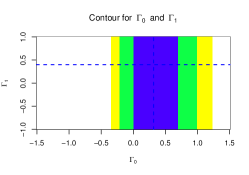
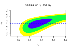
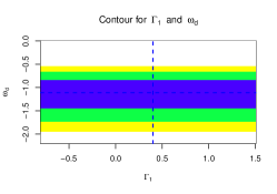
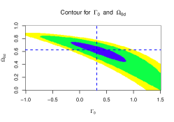
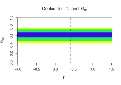
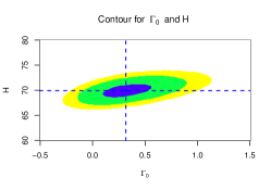
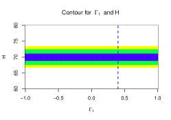
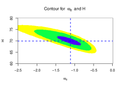
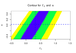
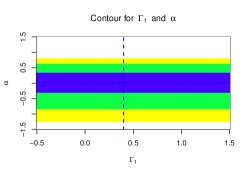
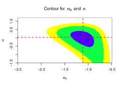
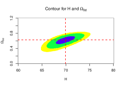
$\Gamma_{0}=0.32,~{}\Gamma_{1}=0.4,~{}\omega_{d}=-1.11,~{}\alpha=0.03,~{}H_{0}=69.92,~{}\Omega_{d}=0.63$. Also $\chi^{2}_{min}=574.812$. So, $\chi^{2}/dof=0.9564(dof=580+27-6=601)$. This model is clearly consistent with the data since $\chi^{2}/dof\approx 1$. It is to be mentioned that for the same data set the best fit values of $\Lambda CDM$ model are obtained as $H_{0}=70.02,\Omega_{0d}=0.73$ with $\chi^{2}_{min}=575.945$. However, as the interaction term $\alpha$ is estimated to be very small, so from a statistical point of view, interaction has no significant effect on the present model. It became evident when we analysed for the non-interacting case, i.e., for $\alpha=0$, and the best fit parameters were obtained as $\Gamma_{0}=0.29,~{}\Gamma_{1}=0.4,~{}\omega_{d}=-1.11,~{}H_{0}=69.92,~{}\Omega_{d}=0.63$, and the minimum value of $\chi^{2}$ = 574.81. Hence, there is a minor difference between the interacting and non-interaction models only for the parameters $\Gamma_{0}$ and $\Omega_{d}$. However, the optimal value of $\chi^{2}$ remained the same for both models. However, to understand relations between the model parameters, a total of thirteen contour plots of $\chi^{2}$ considering it as the function of two parameters (considering the optimal value of other parameters in every scenario) have been drawn. It was utterly fascinating that the $\chi^{2}$ was invariant with $\Gamma_{1}$, and we obtained rectangular contours where $\Gamma_{1}$ was one of the two parameters on which $\chi^{2}$ is dependent. However, $\alpha$ has non-linear relation with DE EoS parameter, whereas with $Gamma_{0}$, it has linear relationship. Now, we use AIC and BIC [113] methods to compare our present model with the $\Lambda CDM$ model. The AIC and BIC are respectively, defined as follows:

$$AIC = -2ln\textit{L}_{max}+2k$$

$$BIC = -2ln\textit{L}_{max}+k~{}lnN$$

where $k,~{}N$ are the number of parameters and number of data points used in the fit. L is maximum likelihood and for Gaussian posterior distribution $\chi^{2}_{min}=-2ln\textit{L}_{max}$. The absolute values of AIC and BIC are not of any interest, only relative value between different models are useful to predict better one compared to other.The AIC and BIC values of our present model and $\Lambda CDM$ model are shown in the Table-I.

Table 1: Model Comparison

	AIC	BIC
Particle creation model	586.812	613.263
$\Lambda CDM$	579.945	588.762

From the Table-1, it is evident that $\Lambda CDM$ model is still best fitted model, but our present model of particle creation is considerably good in terms of compatibility with observational data. This can be perceived more clearly if we calculate the correlation coefficient between the theoretical and observed value of Hubble parameter.

Figure 1: $1\sigma$ (blue), $2\sigma$ (green) and $3\sigma$(yellow) confidence contours between pairs of parameters based on SN Ia+OHV datasets for present particle creation model

Figure 2: $1\sigma$ (blue), $2\sigma$ (green) and $3\sigma$(yellow)$\Gamma_{0d}\sim H$ confidence contour based on SN Ia+OHV datasets for $\Lambda CDM$ model

Figure 3: Graphical representation of  $H-Z$  relation for SN Ia+OHV datasets for $\Lambda CDM$ model

Figure 4: Graphical representation of  $H-Z$  relation for SN Ia+OHV datasets in the present particle creation model

i.e correlation coefficient $r$ between $H_{theo}$ (obtained from equation (21)) and $H_{obs}$. $r$ is calculated from the following equations :

$$r=\frac{\sum_{i=1}^{27}\left(H_{obs}(z_{i})-\bar{H}_{obs}\right)\left(H_{theo}(z_{i})-\bar{H}_{theo}\right)}{(n-1)S_{x}S_{y}}$$ (26)

where $\bar{H}_{obs}$ and $\bar{H}_{theo}$ indicate mean values of observational and theoretical $H(z)$ datasets,respectively and $S_{x},~{}S_{y}$ are given by

$$S_{x} = \sqrt{\frac{\left(H_{obs}(z_{i})-\bar{H}_{obs}\right)^{2}}{n-1}}$$

$$S_{y} = \sqrt{\frac{\left(H_{theo}(z_{i})-\bar{H}_{theo}\right)^{2}}{n-1}}$$

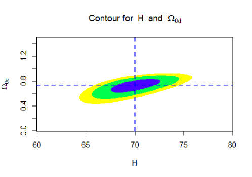
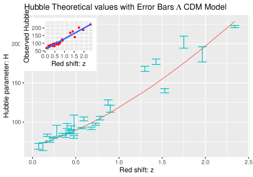
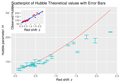
It is to be mentioned that $r$ always lies between -1 and +1. The absolute value of the correlation coefficient, i.e., $|r|$, indicates the relationship strength. To be specific, the larger the absolute value of correlation coefficient, the stronger the linear relationship. $r=0$ indicates no relationship between two variables, while $r=\pm 1$ implies that the points are on a perfect straight line with a positive (negative)slope. Now, for the present model, we have calculated $r=0.965363$ which indicates a strong relationship between $H_{obs}$ and $H_{theo}$. This is also evident from the error diagram Fig. 3) and 4) also. FIGs. 3 and 4 illustrate the evolutionary nature of the cosmic Hubble parameter according to the $\Lambda CDM$ and the particle creation models, respectively, in the 1$\sigma$ confidence region. Note that the circles in FIGs 3 and 4, show the recent observable values. The two plots are pretty similar but deviate at high redshift region. On the other hand, in Fig. 1 and 2, contour plots between different parameters in particle creation and $\Lambda CDM$ model, respectively,, have been shown. It is seen that contour plot for the particle creation model between $\Omega_{od}$ and $H$ is very similar to that of $\Lambda CDM$ model.

IV State finder diagnosis

From the literature, it is evident that almost all theoretical dark energy models can predict the same late-time accelerated expansion ($H>0$ and $q<0$) of the universe. Many difficulties arise in discriminating between them. Then, it is necessary to introduce and study some new quantities (other than the known ones) which can successfully discriminate various DE models at the background level. In this context, a higher order (particularly third order) of the time derivative of the scale factor is introduced, and these would appear as a so-called statefinder parameters $r$ and $s$. The statefinder parameters are defined as the following [80, 81]

$$r\equiv\frac{\dddot{a}}{aH^{3}},$$ (27)

$$s\equiv\frac{r-1}{3(q-\frac{1}{2})}$$ (28)

where the over dot denotes the differentiation with respect to the cosmic time $t$ and $H=\frac{\dot{a}}{a}$ is the Hubble parameter. Furthermore, $q=-\ddot{a}/aH^{2}$ is the decelerating parameter. These parameters are geometrical since they depend on the scale factor. Therefore, the statefinder diagnostic is entirely geometrical diagnostic, and this allows us to characterize the properties of different DE models by finding trajectories in the $s,~{}r$ plane. So, it is a powerful tool that can successfully discriminate between different DE models, even if they predict similar expansion histories. It can be easily verified that for the well-known $\Lambda CDM$ model, the statefinder parameters $\left\{s,r\right\}$ take constant values $\left\{0,1\right\}$ in the s-r plane [80]. Here, we analyze DE models by using statefinder diagnostic tools. We first compute the statefinder parameters in terms of red-shift, then compare them with that of $\Lambda CDM$ and finally, we study their high and low red-shift limits. These operations may provide very fascinating results. For convenience, we introduce the dimensionless Hubble rate $E(z)\equiv H(z)/H_{0}$, where $H_{0}$ is the Hubble constant. Now, the parameters $\left\{q,r,s\right\}$ can be computed in terms of $E(z)$ as follows:

$$q(z)=-1+(1+z)\frac{E_{z}(z)}{E(z)},$$ (29)

$$r(z)=q(z)(1+2q(z))+(1+z)q_{z}(z)$$ (30)

Furthermore $s(z)$ is given by (28), and suffix $z$ stands for derivative with respect to $z$. Using the energy densities expressions in Eqn.(19) and Eqn. (20), one can obtain the analytical expressions of the quantities $E(z)$, $q(z)$, $r(z)$, and $s(z)$.

$$\centering E(z)=(1+z)^{-\frac{\frac{\Gamma_{1}}{H_{0}^{2}}-3-\alpha+\Gamma_{0}}{2}}\left[\Omega_{0m}+\Omega_{0d}(1+z)^{\frac{\Gamma_{1}}{H_{0}^{2}}+3\omega_{d}-\alpha+\Gamma_{0}}\left\{\frac{\alpha\Omega_{0m}}{\Omega_{0d}(\frac{\Gamma_{1}}{H_{0}^{2}}+3\omega_{d}-\alpha+\Gamma_{0})}\left((1+z)^{\left(\frac{\Gamma_{1}}{H_{0}^{2}}+3\omega_{d}-\alpha+\Gamma_{0}\right)}-1\right)+1\right\}\right]^{\frac{1}{2}}\@add@centering$$ (31)

and

$$q(z)=\frac{3(\omega_{d}+1)H_{0}^{2}\Delta+\Omega_{0m}(z+1)^{\alpha}\left\{H_{0}^{2}(3\omega_{d}+\Gamma_{0})+\Gamma_{1}\right\}\left\{H_{0}^{2}(\alpha-\Gamma_{0}+3)-\Gamma_{1}\right\}}{2H_{0}^{2}\left[\Delta+\Omega_{0m}(z+1)^{\alpha}\left\{H_{0}^{2}(3\omega_{d}+\Gamma_{0})+\Gamma_{1}\right\}\right]}-1,$$ (32)

$$r(z)=\frac{(3\omega_{d}+1)(3\omega_{d}+2)H_{0}^{4}\Delta+\Omega_{0m}(z+1)^{\alpha}\left\{H_{0}^{2}(3\omega_{d}+\Gamma_{0})+\Gamma_{1}\right\}\left\{\Gamma_{1}+H_{0}^{2}(-\alpha+\Gamma_{0}-2)\right\}\left\{\Gamma_{1}+H_{0}^{2}(-\alpha+\Gamma_{0}-1)\right\}}{2H_{0}^{4}\left[\Delta+\Omega_{0m}(z+1)^{\alpha}\left\{H_{0}^{2}(3\omega_{d}+\Gamma_{0})+\Gamma_{1}\right\}\right]}$$ (33)

$$s(z)=\frac{2\left(\frac{\left\{9\omega_{d}(\omega_{d}+1)+2\right\}H_{0}^{4}\Delta+\Omega_{0m}(z+1)^{\alpha}\left\{H_{0}^{2}(3\omega_{d}+\Gamma_{0})+\Gamma_{1}\right\}\left\{\Gamma_{1}+H_{0}^{2}(-\alpha+\Gamma_{0}-2)\right\}\left\{\Gamma_{1}+H_{0}^{2}(-\alpha+\Gamma_{0}-1)\right\}}{2H_{0}^{4}\left[\Delta+\Omega_{0m}(z+1)^{\alpha}\left\{H_{0}^{2}(3\omega_{d}+\Gamma_{0})+\Gamma_{1}\right\}\right]}-1\right)}{3\left(\frac{3(\omega_{d}+1)H_{0}^{2}\Delta+\Omega_{0m}(z+1)^{\alpha}\left\{H_{0}^{2}(3\omega_{d}+\Gamma_{0})+\Gamma_{1}\right\}\left\{H_{0}^{2}(\alpha-\Gamma_{0}+3)-\Gamma_{1}\right\}}{H_{0}^{2}\left[\Delta+\Omega_{0m}(z+1)^{\alpha}\left\{H_{0}^{2}(3\omega_{d}+\Gamma_{0})+\Gamma_{1}\right\}\right]}-3\right)}$$ (34)

where $\Delta=(z+1)^{\left(3\omega_{d}+\Gamma_{0}+\frac{\Gamma_{1}}{H_{0}^{2}}\right)}\left[H_{0}^{2}\left\{\Omega_{0d}(-\alpha+3\omega_{d}+\Gamma_{0})-\alpha\Omega_{0m}\right\}+\Omega_{0d}\Gamma_{1}\right]$
We shall now describe the behavior of the parameters $q,r,s$ numerically in plotting the evolutionary trajectories of the statefinder parameters in the s-r and q-r plane for our model. To plot all the figures we set the following best fit values of the model parameters as,
$\Gamma_{0}=0.32,~{}\Gamma_{1}=0.4,~{}\alpha=0.03,~{}H_{0}=69.92,~{}\Omega_{0d}=0.63,~{}\Omega_{0m}=0.37$ and
(I)  $\omega_{d}=-1.11$ for figures (5), (8),
(II)  $\omega_{d}=-1$ for figures (6), (9),
(III)  $\omega_{d}=-0.85$ for figures (7), (10).

Figure 5: The figures show different time evolution trajectories of the state finder pair $(s,r)$ for this model using the dataset, as indicated above in each panel. In panel $(a)$, the interaction parameter $\alpha$ is changing but $\Gamma_{0}$ and $\Gamma_{1}$ are fixed as $\Gamma_{0}=0.32$ and $\Gamma_{1}=0.4$. In panel $(b)$, the parameter $\Gamma_{0}$ is changing but $\alpha$ and $\Gamma_{1}$ are fixed as $\alpha=0.03$ and $\Gamma_{1}=0.4$. In panel $(c)$, the parameter $\Gamma_{1}$ is changing but $\alpha$ and $\Gamma_{0}$ are fixed as $\alpha=0.03$ and $\Gamma_{0}=0.32$. In each panel, the colored circles denote the present value of the state finder parameter $(s_{0},r_{0})$ and the blue star corresponds to the $\Lambda CDM$ model.

Figure 6: The figures show different time evolution trajectories of the state finder pair $(s,r)$ for this model using the dataset, as indicated above in each panel. In panel $(a)$, the interaction parameter $\alpha$ is changing but $\Gamma_{0}$ and $\Gamma_{1}$ are fixed as $\Gamma_{0}=0.32$ and $\Gamma_{1}=0.4$. In panel $(b)$, the parameter $\Gamma_{0}$ is changing but $\alpha$ and $\Gamma_{1}$ are fixed as $\alpha=0.03$ and $\Gamma_{1}=0.4$. In panel $(c)$, the parameter $\Gamma_{1}$ is changing but $\alpha$ and $\Gamma_{0}$ are fixed as $\alpha=0.03$ and $\Gamma_{0}=0.32$. In each panel, the colored circles denote the present value of the state finder parameter $(s_{0},r_{0})$ and the blue star corresponds to the $\Lambda CDM$ model.

Figure 7: The figures show different time evolution trajectories of the state finder pair $(s,r)$ for this model using the dataset, as indicated above in each panel. In panel $(a)$, the interaction parameter $\alpha$ is changing but $\Gamma_{0}$ and $\Gamma_{1}$ are fixed as $\Gamma_{0}=0.32$ and $\Gamma_{1}=0.4$. In panel $(b)$, the parameter $\Gamma_{0}$ is changing but $\alpha$ and $\Gamma_{1}$ are fixed as $\alpha=0.03$ and $\Gamma_{1}=0.4$. In panel $(c)$, the parameter $\Gamma_{1}$ is changing but $\alpha$ and $\Gamma_{0}$ are fixed as $\alpha=0.03$ and $\Gamma_{0}=0.32$. In each panel, the colored circles denote the present value of the state finder parameter $(s_{0},r_{0})$ and the blue star corresponds to the $\Lambda CDM$ model.

Figure 8: The figures show different time evolution trajectories of the parameter pair $(q,r)$ for this model using the dataset, as indicated above in each panel. In panel $(a)$, the interaction parameter $\alpha$ is changing but $\Gamma_{0}$ and $\Gamma_{1}$ are fixed as $\Gamma_{0}=0.32$ and $\Gamma_{1}=0.4$. In panel $(b)$, the parameter $\Gamma_{0}$ is changing but $\alpha$ and $\Gamma_{1}$ are fixed as $\alpha=0.03$ and $\Gamma_{1}=0.4$. In panel $(c)$, the parameter $\Gamma_{1}$ is changing but $\alpha$ and $\Gamma_{0}$ are fixed as $\alpha=0.03$ and $\Gamma_{0}=0.32$. In each panel, the colored circles denote the present value of the state finder parameter $(q_{0},r_{0})$ and the blue star corresponds to the $de~{}Sitter$ model.

Figure 9: The figures show different time evolution trajectories of the parameter pair $(q,r)$ for this model using the dataset, as indicated above in each panel. In panel $(a)$, the interaction parameter $\alpha$ is changing but $\Gamma_{0}$ and $\Gamma_{1}$ are fixed as $\Gamma_{0}=0.32$ and $\Gamma_{1}=0.4$. In panel $(b)$, the parameter $\Gamma_{0}$ is changing but $\alpha$ and $\Gamma_{1}$ are fixed as $\alpha=0.03$ and $\Gamma_{1}=0.4$. In panel $(c)$, the parameter $\Gamma_{1}$ is changing but $\alpha$ and $\Gamma_{0}$ are fixed as $\alpha=0.03$ and $\Gamma_{0}=0.32$. In each panel, the colored circles denote the present value of the state finder parameter $(q_{0},r_{0})$ and the blue star corresponds to the $de~{}Sitter$ model.

Figure 10: The figures show different time evolution trajectories of the parameter pair $(q,r)$ for this model using the dataset, as indicated above in each panel. In panel $(a)$, the interaction parameter $\alpha$ is changing but $\Gamma_{0}$ and $\Gamma_{1}$ are fixed as $\Gamma_{0}=0.32$ and $\Gamma_{1}=0.4$. In panel $(b)$, the parameter $\Gamma_{0}$ is changing but $\alpha$ and $\Gamma_{1}$ are fixed as $\alpha=0.03$ and $\Gamma_{1}=0.4$. In panel $(c)$, the parameter $\Gamma_{1}$ is changing but $\alpha$ and $\Gamma_{0}$ are fixed as $\alpha=0.03$ and $\Gamma_{0}=0.32$. In each panel, the colored circles denote the present value of the state finder parameter $(q_{0},r_{0})$ and the blue star corresponds to the $de~{}Sitter$ model.

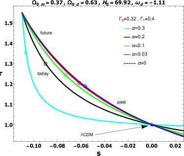
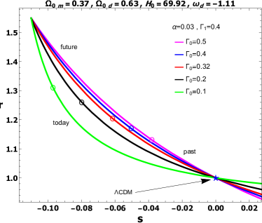
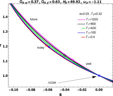
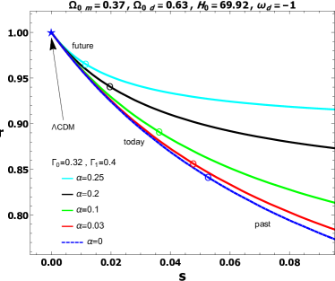
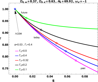
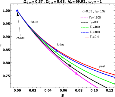
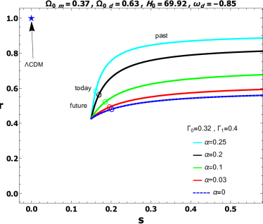
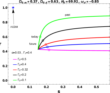
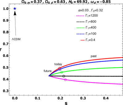
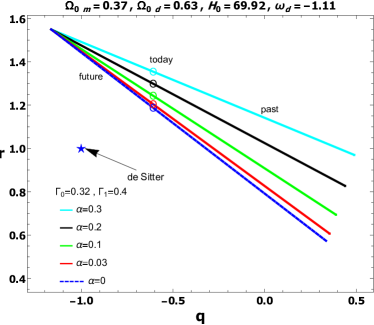
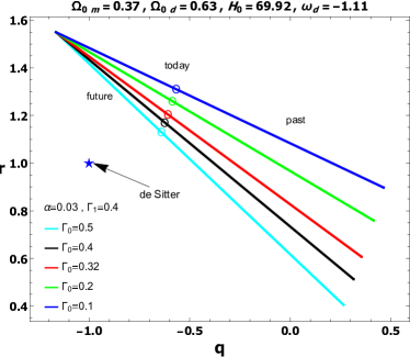
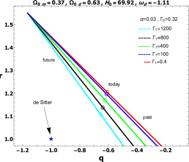
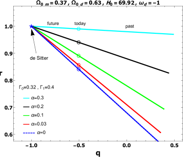
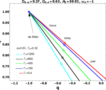
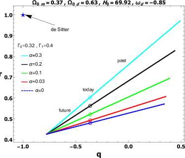
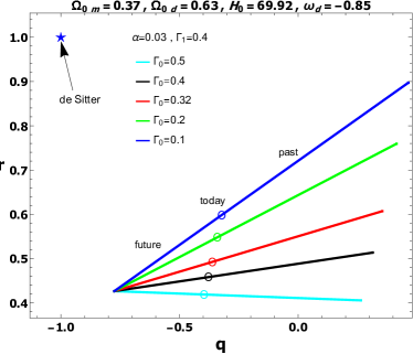
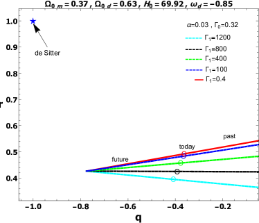
The evolutionary trajectories are plotted in the $s-r$ plane for different values of the coupling parameter of the interaction term $\alpha$ in (5, 6, 7), for different values of parameter $\Gamma_{0}$ in (5, 6, 7) and for different values of $\Gamma_{1}$ in (5, 6, 7). Note that for drawing each figure, we only vary one parameter keeping all other parameters fixed. In all diagrams (5), (6), and (7), the blue star symbol indicates the standard $\Lambda CDM$ fixed point. The present value of the state finder pair $(s,~{}r)$ are shown by the putting colored circles.
In figures 5, 6, and 7, we obtain different trajectories in $s-r$ plane for different values of the interaction parameter $\alpha$. When $\alpha$ is increasing, then $s$ is decreasing, and $r$ is increasing. The scenario shows that the present values of the statefinder pair $(s,r)$ are moving away from the standard $\Lambda CDM$ fixed point at an earlier time (in figure 5), moving towards $\Lambda CDM$ fixed point (in figure 6) in the future but not even evolving around $\Lambda CDM$ fixed point (in figure 7). Therefore, the evolutionary trajectories show that evolution starts from $\Lambda CDM$ point at early times and after that, moving towards the direction of $r$ increasing and $s$ decreasing (in figure 5). In figure 6, when $\alpha$ increases, $s$ will decrease, and $r$ will increase, then the evolutionary trajectories reach $\Lambda CDM$ fixed point. But, in figure 7, the scenario will not be achieved. Therefore, $\alpha$ affects on the evolutionary trajectories in the $s-r$ plane.
In figures 5, 6 and 7, we obtain different trajectories in the $s-r$ plane by taking different values of the parameter $\Gamma_{0}$. As $\Gamma_{0}$ decreases, the value of $s$ decreases, and $r$ increases. So, the present values of the statefinder pair $(s,r)$ are moving away from the standard $\Lambda CDM$ fixed point at the earlier time (in figure 5), and moving towards $\Lambda CDM$ fixed point (in figure 6), but not evolved around $\Lambda CDM$ fixed point (in figure 7). Therefore, the evolutionary trajectories show that evolution starts from $\Lambda CDM$ point at early times, and after that, the trajectories moving towards the direction of $r$ increasing and $s$ decreasing (see in figure 5). In figure 6, when $\Gamma_{0}$ decreases, $s$ decreases and $r$ increases, then finally, the evolutionary trajectories reach $\Lambda CDM$ fixed point. However, 7 shows that the scenario does not happen. So, $\Gamma_{0}$ also affects the evolutionary trajectories in the $s-r$ plane.
In figures 5, 6, and 7, different trajectories in the s-r plane are obtained for different values of the interaction parameter $\Gamma_{1}$. As the value of $\Gamma_{1}$ decreases, the value of $s$ decreases, and $r$ increases. So, the present values of the statefinder pair $(s,r)$ are moving away from the standard $\Lambda CDM$ fixed point at an earlier time (see in figure 5), and moving towards $\Lambda CDM$ fixed point (in figure 6), but not evolved around the $\Lambda CDM$ fixed point (see in figure 7) when $\Gamma_{1}$ decreases. Therefore, the evolutionary trajectories show that evolution starts from $\Lambda CDM$ point at early times and after that going towards when $r$ increases and $s$ decreases (see in figure 5). In figure 6, when $\Gamma_{1}$ decreases, then $s$ decreases and $r$ increases. Then finally the evolutionary trajectories reach $\Lambda CDM$ fixed point. But, the figure 7 shows that the scenario does not happen. So, $\Gamma_{1}$ can also affect the evolutionary trajectories in the s-r plane.
The evolutionary trajectories are plotted in the q-r plane for different values of interaction coupling parameter $\alpha$ in (8, 9, 10), for different values of parameter $\Gamma_{0}$ in (8, 9, 10) and for different values of $\Gamma_{1}$ in (8, 9, 10). That is, we make changes to only one parameter, keeping all others unaltered. In all diagrams (8), (9) and (10), the blue star symbol denotes the standard $de~{}Sitter$ fixed point. The present value of the pair $(q,r)$ is shown with the colored circles.
In figures 8, 9, and 10, the trajectories in the q-r plane for different values of the interaction coupling parameter $\alpha$ are obtained. As the value of $\alpha$ increases, the value of $q$ decreases, and $r$ increases. So, the present values of the statefinder pair $(q,r)$ are moving towards $de~{}Sitter$ fixed point (see in figure 9) but not evolve around $de~{}Sitter$ fixed point (in figures 8, 10) as the value of $\alpha$ increases. Therefore, in figure 9, $q$ decreases and $r$ increases with the increasing value of $\alpha$, and finally, the evolutionary trajectories reach the $de~{}Sitter$ fixed point. But, in figures 8, and 10, this type of scenario is not happened. So, $\alpha$ can affect the evolutionary trajectories in the q-r plane.
In figures 8, 9 and 10, we get different trajectories in q-r plane for different values of the parameter $\Gamma_{0}$. As the value of $\Gamma_{0}$ increases, $q$ and $r$ decrease simultaneously. So, the present values of the statefinder pair $(q,r)$ are moving towards $de~{}Sitter$ fixed point in figure 9 in future but not even evolving around $de~{}Sitter$ fixed point in figures 8, 10 as the value of $\Gamma_{0}$ increases. Therefore, in figure 9, $q$ and $r$ decrease with the increasing value of $\Gamma_{0}$, and finally, the evolutionary trajectories reach to $de~{}Sitter$ fixed point. But, in figures 8, and 10, this type of scenario can not happen. So, $\Gamma_{0}$ can affect the evolutionary trajectories in q-r plane.

In figures 8, 9, and 10, we get different trajectories in the q-r plane for different values of the parameter $\Gamma_{1}$. As the value of $\Gamma_{1}$ increases, $q$ and $r$ decrease simultaneously. So, the present values of the statefinder pair $(q,r)$ are moving towards the $de~{}Sitter$ fixed point in figure 9 in future but not even evolving around $de~{}Sitter$ fixed point in figures 8, 10 as the value of $\Gamma_{1}$ increases. Therefore, in figure 9, $q$ and $r$ decrease with the increasing value of $\Gamma_{1}$, and finally, the evolutionary trajectories reach the $de~{}Sitter$ fixed point. But, in figures 8 and 10, this type of scenario can not happen. So, $\Gamma_{1}$ can affect the evolutionary trajectories in q-r plane. The present value of $(q,r)$ can be important if it be extracted from some future experiments.

V Dynamical analysis

This section will discuss the critical points analysis for the model under consideration. We first convert the cosmological evolution equations into an autonomous system of ordinary differential equations by adopting suitable transformation of variables. After extracting the critical points from the autonomous system, we find the nature of critical points by evaluating the eigenvalues of the linearized Jacobian matrix at the critical points. Further, the cosmological behavior of the critical points shall be explored via the cosmological parameters evaluated at critical points.
We consider the following dimensionless variables as the dynamical variables

$$x=\frac{\rho_{d}}{3H^{2}}~{}~{},~{}~{}y=\frac{p_{d}}{3H^{2}}$$ (35)

which are normalized over Hubble scale. By using these variables, the governing equations, namely, constraint equation (4), acceleration equation (12) and conservation equations (7) and (13) give the following system of first-order ordinary differential equations with the creation pressure in Eqn. (11)

$$\begin{split}\frac{dx}{dN}&=\frac{Q}{3H^{3}}-(1-x)\left\{3y+x\left(\Gamma_{0}+\frac{\Gamma_{1}}{H^{2}}\right)\right\},&\\ \frac{dy}{dN}&=\frac{y}{x}\left[\frac{Q}{3H^{3}}-(1-x)\left\{3y+x\left(\Gamma_{0}+\frac{\Gamma_{1}}{H^{2}}\right)\right\}\right],&\\ &~{}~{}\end{split}$$ (36)

The system of ODEs in Eqn. (LABEL:ode_system) is not an autonomous system system due to presence of interaction $Q$ and Hubble function $H$ in its expressions. By using interaction term in (8) and considering a new variable $z=\frac{H_{0}}{H^{2}}$, where $H_{0}$ is constant, in the above system, we obtain the following autonomous system of ODEs (taking $H_{0}=1$):

$$\begin{split}\frac{dx}{dN}&=(1-x)\left\{\alpha-3y-x(\Gamma_{0}+\Gamma_{1}z)\right\},&\\ \frac{dy}{dN}&=\frac{y}{x}(1-x)\left\{\alpha-3y-x(\Gamma_{0}+\Gamma_{1}z)\right\},&\\ \frac{dz}{dN}&=3z\left\{1+y-\frac{(1-x)(\Gamma_{0}+\Gamma_{1}z)}{3}\right\},&~{}~{}\end{split}$$ (37)

where $N=\ln a$ is the e-folding parameter taken to be independent variable. Cosmological parameters associated to this model can immediately be expressed in terms of dynamical variables as follows :
The density parameters for dark energy and dark matter are

$$\Omega_{d}=x,$$ (38)

and

$$\Omega_{m}=1-x$$ (39)

respectively. The equation of state parameter for dark energy is

$$\omega_{d}=\frac{p_{d}}{\rho_{d}}=\frac{y}{x}$$ (40)

and the effective equation of state parameter for the model is

$$\omega_{eff}=y-(1-x)\left(\frac{\Gamma_{0}+\Gamma_{1}z}{3}\right).$$ (41)

and the deceleration parameter for the model takes the form

$$q=-1+\frac{3}{2}(1+\omega_{eff})=-1+\frac{3}{2}\left\{1+y-(1-x)\left(\frac{\Gamma_{0}+\Gamma_{1}z}{3}\right)\right\}$$ (42)

which shows the condition for acceleration of the universe $q<0\Longrightarrow\omega_{eff}<-\frac{1}{3}$ and for deceleration $q>0\Longrightarrow\omega_{eff}>-\frac{1}{3}.$
Moreover, the evolution equation of the Hubble expansion function reads as:

$$\frac{\dot{H}}{H^{2}}=-\frac{3}{2}\left\{1+y-(1-x)\left(\frac{\Gamma_{0}+\Gamma_{1}z}{3}\right)\right\}.$$ (43)

V.1 Critical points and cosmological analysis of the autonomous system (LABEL:autonomous_system1):

We shall now discuss the of critical points and their corresponding physical parameters and stability in the phase space of $3D$ autonomous system (LABEL:autonomous_system1).
The critical points extracted from the system (LABEL:autonomous_system1) are the following

• I. Set of critical points : $A=(1,y_{c},0)$

• II. Set of critical points : $B=(1,-1,z_{c})$

• III. Set of critical points : $C=\left(x_{c},\frac{\alpha-x_{c}\Gamma_{0}}{3},0\right)$

• IV. Set of critical Points : $D=\left(x_{c},\frac{\alpha-x_{c}(\alpha+3)}{3},\frac{3+\alpha-\Gamma_{0}}{\Gamma_{1}}\right)$

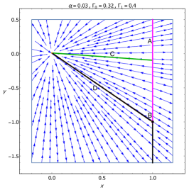
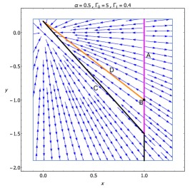
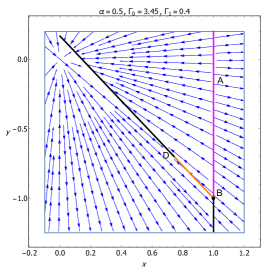
Note that all the sets are non-isolated sets of points in the phase space. Set of critical points and their corresponding physical parameters are shown in the table (2) and the eigenvalues of linearized Jacobian matrix are presented in the Table 3.

Table 2: The critical points and the corresponding physical parameters are presented.

Critical Points	$\mathbf{Existence}$	$\mathbf{\Omega_{m}}$	$\mathbf{\Omega_{d}}$	$\mathbf{\omega_{d}}$	$\mathbf{\omega_{eff}}$	$q$
$A$	Always	$0$	$1$	$y_{c}$	$y_{c}$	$\frac{1}{2}+\frac{3y_{c}}{2}$
$B$	Always	$0$	$1$	$-1$	$-1$	$-1$
$C$	$0\leq x_{c}\leq 1$	$1-x_{c}$	$x_{c}$	$\frac{\alpha-x_{c}\Gamma_{0}}{3x_{c}}$	$\frac{\alpha-\Gamma_{0}}{3}$	$~{}~{}\frac{1}{2}(\alpha-\Gamma_{0}+1)$
$D$	$0\leq x_{c}\leq 1~{}~{}\mbox{and}~{}~{}\Gamma_{1}\neq 0$	$1-x_{c}$	$x_{c}$	$\frac{\alpha-x_{c}(\alpha+3)}{3x_{c}}$	$-1$	$-1$

Table 3: The eigenvalues of the linearized system (LABEL:autonomous_system1) are presented where $\Sigma=(\sqrt{(x_{c}-1)}\left\{x_{c}^{3}(\alpha-\Gamma_{0}+3)^{2}+x_{c}^{2}(\alpha-\Gamma_{0}+3)(\alpha+\Gamma_{0}-3)-\alpha^{2}+\alpha x_{c}(3\alpha-2\Gamma_{0}+6)\right\}\overline{}$

Critical Points	$\mathbf{\lambda_{1}}$	$\mathbf{\lambda_{2}}$	$\mathbf{\lambda_{3}}$
$A$	$0$	$3(y_{c}+1)$	$\Gamma_{0}-\alpha+3y_{c}$
$B$	$0$	$0$	$\Gamma_{0}+z_{c}\Gamma_{1}-\alpha-3$
$C$	$0$	$\frac{x_{c}\alpha-\alpha}{x_{c}}$	$\alpha-\Gamma_{0}+3$
$D$	$0$	$\frac{(x_{c}-1)\left\{x_{c}(\alpha-\Gamma_{0}+3)+\alpha\right\}-\Sigma}{2x_{c}}$	$\frac{(x_{c}-1)\left\{x_{c}(\alpha-\Gamma_{0}+3)+\alpha\right\}+\Sigma}{2x_{c}}$

Figure 11: The figures show the phase space projection of the autonomous system (LABEL:autonomous_system1) on the x-y plane. In panel (a) phase plot has been drawn for the parameter values $\alpha=0.03$, $\Gamma_{0}=0.32$ and $\Gamma_{1}=0.4$. In panel (b) phase plot has been drawn for the parameter values $\alpha=0.5$, $\Gamma_{0}=5$ and $\Gamma_{1}=0.4$. In panel (c) phase plot has been drawn for the parameter values $\alpha=0.5$, $\Gamma_{0}=3.45$ and $\Gamma_{1}=0.4$. In all panels, the magenta colored line represents the set of points A, the green colored line represents the set of points C, the orange colored line represents the set of points D. The black dotted line on a line represent the stable portion on that line. The point B is unstable in all the figures.

Figure 12: The figures show the phase space projection of perturbation of the autonomous system (LABEL:autonomous_system1) along the x,y and z axes for the set of critical points $B$ for parameter values $\alpha=0.03$, $\Gamma_{0}=0.32$ and $\Gamma_{1}=0.4$. In panel (a) perturbations come back but in panels (b), (c) perturbations do not come back. This indicates that the set $B$ is unstable for parameters value $\alpha=0.03$, $\Gamma_{0}=0.32$ and $\Gamma_{1}=0.4$.

Figure 13: Figures show that the evolution of cosmological parameters like the DE density parameter $\Omega_{d}$, the density parameter for DM $\Omega_{m}$, the equation of state parameter $\omega_{d}$, the effective equation of state parameter $\omega_{eff}$, and the decelerating parameter $q$ with respect to $N=\ln a$ of the autonomous system (LABEL:autonomous_system1) with the parameter values $\alpha=0.03$, $\Gamma_{0}=0.32$ and $\Gamma_{1}=0.4$. In panel (a) Numerical investigation shows that the ultimate fate of the universe is late time accelerated evolution in cosmological constant era followed by an intermediate matter dominated phase with initial values $x(0)=0.7,y(0)=-0.7,z(0)=0$ and in panel (b) Numerical investigation shows that the ultimate fate of the universe is late time accelerated evolution in phantom era followed by an intermediate matter dominated phase with initial values $x(0)=0.7,y(0)=-1.3,z(0)=0$.

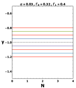
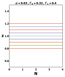
• The set of critical points $A$ represents a completely dark energy dominated ($\Omega_{d}=1$) solution where DE mimics any perfect fluid model since $\omega_{d}=y_{c}$ (see Table 2) and $y_{c}$ takes any real value. Depending upon $y_{c}$, DE can behave as quintessence, cosmological constant, and phantom fluid, respectively, according to $-1<y_{c}<-\frac{1}{3}$, $y_{c}=-1$ and $y_{c}<-1$ in the phase space. It should be mentioned that the DE can mimic dust fluid for $y_{c}=0$. However, there exists an accelerating phase only for $y_{c}<-\frac{1}{3}$. From Table 3, we observe that the set has precisely one vanishing eigenvalue, so by definition, it is a normally hyperbolic set, and the stability of this set can be found by evaluating the signature of remaining non-vanishing eigenvalues. The set is stable for

  $$y_{c}<\mbox{min}\left\{-1,~{}~{}\frac{\alpha-\Gamma_{0}}{3}\right\}.$$

  From the stability condition, one may conclude that the set of points $A$ is stable only in the phantom regime where DE behaves as a phantom fluid. Therefore, a DE-dominated accelerated Universe is always observed by the set $A$ where the Universe is evolving in phantom regime only. On the other hand, a decelerated dust-dominated Universe is achieved when the DE behaves as dust. Here, the point with coordinate (1,0,0) on the set is an unstable saddle-like solution.

• Set of critical points $B$ exists for all parameter values. It is completely DE dominated and DE behaves as cosmological constant. Acceleration is always possible for this set. It is non-hyperbolic set. Since two of its eigenvalues having zero real part, it is not a normally hyperbolic set. Therefore, its stability can be checked by numerical investigation and is done in the fig. (12). Figure shows that the trajectories are attracted only in one direction.
  

• Set of critical points $C$ exists for $0\leq x_{c}\leq 1$. It represents a scaling solution in the phase space with the combination of both DE and DM, and the ratio is $\Omega_{d}/\Omega_{m}=x_{c}/(1-x_{c})$. Here, DE behaves as perfect fluid in nature. Acceleration of the Universe exists for $\alpha<\Gamma_{0}-1$. The phantom behavior is obtained for $\alpha<\Gamma_{0}-3$. It is a non-hyperbolic set with exactly one vanishing eigenvalue, so the set is normally hyperbolic set. Therefore, the set $C$ is stable for $\left(0<x_{c}<1~{}~{}\mbox{and}~{}~{}0<\alpha<\Gamma_{0}-3\right)$. Therefore, late time accelerated universe is obtained by the set and the Universe evolves in the phantom regime.
  

• Set of point $D$ exists for all parameter values with $\Gamma_{1}\neq 0$. It is also a solution with the combination of both the DE and DM with the ratio $\Omega_{d}/\Omega_{m}=x_{c}/(1-x_{c})$. It may be a scaling solution at late times. DE behaves as perfect fluid in nature. Accelerating universe exists for this set. The set of critical points $D$ is also non-hyperbolic. Moreover, the set is normally hyperbolic. The set of critical points $D$ is stable for $\left\{0<x_{c}<1~{}~{}\mbox{and}~{}~{}\left(\frac{\left(x_{c}^{3/2}+x_{c}+\sqrt{x_{c}}-1\right)\alpha}{x_{c}^{3/2}+x_{c}}+3\leq\Gamma_{0}<\alpha+3~{}~{}\mbox{or}~{}~{}\frac{\left(x_{c}^{3/2}-x_{c}+\sqrt{x_{c}}+1\right)\alpha}{x_{c}-x_{c}^{3/2}}+\Gamma_{0}\leq 3\right)~{}~{}\mbox{and}~{}~{}\Gamma_{1}\neq 0~{}~{}\mbox{and}~{}~{}\alpha>0\right\}$.

V.2 Cosmology of the critical points

Late time accelerated evolution of the Universe is achieved by a set $A$ where the Universe is evolving in the phantom phase and is entirely dominated by phantom fluid ($y_{c}<-1$). The fig. 11 shows that the set of points $A$ is a stable attractor in the phantom regime. On the other hand, dust dominated decelerated Universe can be observed by the set when the DE behaves as dust $y_{c}=0$, which describes the matter dominated intermediate phase of the Universe. Some trajectories are attracted towards the set, and others are coming out from the set. Therefore, it is a saddle-like solution.

The set $B$ corresponds to the accelerated Universe, and acceleration is driven by the cosmological constant. Unfortunately, it does not represent the late-time solution. Numerical investigation in fig (12) confirms the instability of this set in phase space. Therefore, it is not so physically interesting set.

The set $C$ represents the late-time scaling attractor on some parameter restrictions. For $0<\alpha<\Gamma_{0}-3$ in $0<x_{c}<1$, the set $C$ corresponds to late time scaling attractor, which represents the accelerated Universe evolving in phantom regime with $0<\Omega_{d}<1$, and $0<\Omega_{m}<1$ solving the coincidence problem. The fig. 11 shows that the set $C$ exhibiting the late-time scaling attractor evolving in phantom regime.

The set $D$ corresponds to the late time cosmological constant-dominated accelerated universe. For $\alpha>\Gamma_{0}-3$ with $\Gamma_{1}\neq 0$, it also represents the scaling attractor with $0<\Omega_{d}<1$ and $0<\Omega_{m}<1$. Moreover, it can alleviate the coincidence problem successfully. This type of solution is also obtained in ref [102] when particle creation rate $\Gamma=\Gamma_{0}H$. However, the solution in that case could not solve the coincidence problem. Here, the Universe continuously evolves in cosmological constant era. The figures (11) and (11) confirm the stability of the set $D$ in the phase space.

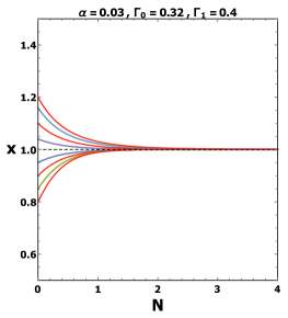
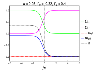
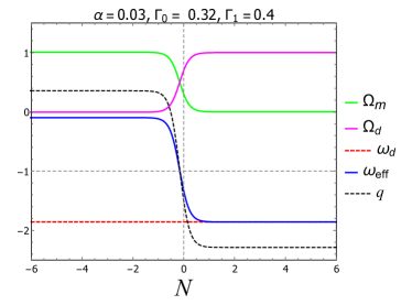
The evolution of cosmological parameters is shown in the figure (13) where the density parameter for DE ($\Omega_{d}$), density parameter for DM ($\Omega_{m}$), equation of state parameter for DE ($\omega_{d}$), the effective equation of state parameter ($\omega_{eff}$), and deceleration parameter ($q$) are plotted against the e-folding parameter $N=\ln a$ with suitable initial conditions. Depending on fine tuning of initial conditions, subfigure (13) shows that the late time accelerated evolution of the Universe is depicted in the cosmological constant era, whereas the subfigure (13) exhibits the accelerating late phase of the Universe attracted in the phantom regime.

VI Thermodynamical Analysis of Energy transfer between the dark sectors of the matter distribution due to particle creation

The particle creation mechanism gives rise to an energy transfer between the dark species causing the two subsystems to have different temperatures, and as a result, thermodynamics of irreversible process comes into the picture. Starting from Euler’s thermodynamical relation $nTs=\rho+p$ and using the energy conservation equations (6) and (7) along with the modified particle number conservation relations (9) and (10) for the two dark subsystems, the evolution equations for the temperatures of the individual dark fluid elements read as

$$\frac{\dot{T}_{m}}{T_{m}}=-\alpha H$$ (44)

and

$$\frac{\dot{T}_{d}}{T_{d}}=-3H\omega_{d}-\alpha H\frac{\rho_{m}}{\rho_{d}}$$ (45)

Here $T_{m},T_{d}$ are temperatures of DM and DE respectively. Integrating the above equations we obtain

$$T_{m}=T_{0}\left(\frac{a}{a_{0}}\right)^{-2-\alpha}$$ (46)

and

$$T_{d}=T_{0}\left(\frac{a}{a_{0}}\right)^{-3\omega_{d}}\left\{\frac{\alpha r_{0}}{\eta}\left(\left(\frac{a}{a_{0}}\right)^{\eta}-1\right)+1\right\}$$ (47)

where  $T_{0}$  is the common temperature of the two subsystems in equilibrium configuration. It is to be noted that in deriving equation (46) one has to take into account of the temperature  $T_{m_{0}}\propto a^{-2}$  for the DM sector in the absence of interaction.
However, in presence of interaction, when the temperature of the system differs from that of the horizon, there will be spontaneous heat flow between the horizon and the fluid components, and hence there will no longer be any thermal equilibrium. As we are considering the universe bounded by the apparent horizon as an isolated system, so at the thermal equilibrium, the common temperature  $T_{0}$  is nothing but the Hawking temperature at the horizon i.e.  $T_{0}=\frac{1}{2\pi R_{A}}$  where  $R_{A}$  is the radius of the apparent horizon for the FRW model. In case of a flat universe $R_{A}=\frac{1}{H}$
For the present isolated system, if we denote the entropies of the two subsystems as  $S_{m}$  and  $S_{d}$  and  $S_{E}$  is the entropy of the bounding event horizon, then

$$T_{m}\frac{dS_{m}}{dt}=\frac{dQ_{m}}{dt}=\frac{dE_{m}}{dt}$$ (48)

and

$$T_{d}\frac{dS_{d}}{dt}=\frac{dQ_{d}}{dt}=\frac{dE_{d}}{dt}+p_{d}\frac{dV}{dt}$$ (49)

while from the Bekenstein area formula,

$$\frac{dS_{A}}{dt}=2\pi R_{A}\dot{R_{A}}$$ (50)

Here  $V=\frac{4}{3}\pi R_{A}^{3}$  is the volume of the Universe bounded by the apparent horizon and  $E_{m}=\rho_{m}V$  and  $E_{d}=\rho_{d}V$.
As the overall system is isolated so the heat flow across the horizon  $Q_{h}$  will satisfy

$$\dot{Q_{h}}=-\left(\dot{Q_{m}}+\dot{Q_{d}}\right)$$ (51)

In equilibrium configuration, the entropy of the whole system depends on the energy densities and volume only. Furthermore, from the extensive property, it is just the sum of the entropies, i.e.  $S_{m}+S_{d}+S_{E}$. However in non-equilibrium thermodynamics, one has to take into account the irreversible fluxes such as energy transfers in the total entropy, and hence the time variation of the total entropy is given by []

$$\frac{dS_{T}}{dt}=\frac{dS_{m}}{dt}+\frac{dS_{d}}{dt}+\frac{dS_{A}}{dt}-A_{d}\dot{Q_{d}}\ddot{Q_{d}}-A_{h}\dot{Q_{h}}\ddot{Q_{h}}$$ (52)

where $A_{d}$ and $A_{h}$ are the energy transfer constants between DE and DM within the Universe and between the Universe and the horizon respectively. Now using equations (48) - (50) the explicit form of different terms on the r.h.s of equation (52) are given by

$$\frac{dS_{m}}{dt}=3\pi H^{-1}\Omega_{m}\left(\frac{a}{a_{0}}\right)^{\alpha+2}\left(\frac{\Gamma}{3H}-\frac{\alpha}{3}+q\right)$$ (53)

$$\frac{dS_{d}}{dt}=3\pi H^{-1}\Omega_{d}\left(\frac{a}{a_{0}}\right)^{3\omega_{d}}\frac{1}{\left\{\frac{\alpha r_{0}}{\eta}\left(\left(\frac{a}{a_{0}}\right)^{\eta}-1\right)+1\right\}}\left[q(1+\omega_{d})+\frac{\alpha}{3}\left(\frac{1}{\Omega_{d}}-1\right)\right]$$ (54)

$$\frac{dS_{A}}{dt}=2\pi H^{-1}(1+q)$$ (55)

$$A_{d}\dot{Q_{d}}\ddot{Q_{d}}=\frac{3A_{d}}{4}\left[\alpha+3\Omega_{d}\left\{q(1+\omega_{d})-\frac{\alpha}{3}\right\}\right]\left[\dot{\Omega_{d}}\left\{q(1+\omega_{d})-\frac{\alpha}{3}\right\}+\dot{q}(1+\omega_{d})\Omega_{d}\right]$$ (56)

$$A_{h}\dot{Q_{h}}\ddot{Q_{h}}=\frac{3A_{h}}{4}\left[3q(1+\omega_{d}\Omega_{d})+\Gamma\Omega_{m}H^{-1})\right]\left[\dot{q}(1+\omega_{d}\Omega_{d})+\dot{\Omega_{d}}\left(q\omega_{d}-\frac{\Gamma H^{-1}}{3}\right)+\frac{H^{-1}}{3}\left\{\Gamma+2\Gamma_{1}\Omega_{m}(1+q)\right\}\right]$$ (57)

where $\Omega_{m},\Omega_{d}$ denote energy density parameters of DM and DE respectively given by
$\Omega_{m}=\frac{\rho_{m}}{3H^{2}},~{}~{}\Omega_{d}=\frac{\rho_{d}}{3H^{2}}$ and $q=-1-\frac{\dot{H}}{H^{2}}$ being the deceleration parameter.
$\dot{\Omega_{d}}$ and $\dot{q}$ are given by

$$\dot{\Omega_{d}}=H\left[\Omega_{d}(2q-3\omega_{d}-1-\alpha)+\alpha\right]$$ (58)

$$\dot{q}=H\left[(j+3q+2)+2(1+q)^{2}\right]$$ (59)

where $j=\frac{\ddot{H}}{H^{3}}-3q-2$ denotes jerk parameter. As the expression for  $\frac{dS_{T}}{dt}$  is very lengthy, so to get an idea about its sign we make use of the estimated values of different parameters at present epoch (i.e a=1)from section 3 as follows[]:
$\omega_{0d}=-1.11,~{}~{}\Omega_{0d}=0.62,~{},~{}H_{0}=69.92,~{}\Gamma_{0}=0.32,\Gamma_{1}=0.4,\alpha=0.03$ and from these best fit values of the parameters we eventually obtain present estimated values of other parameters such as $q=-0.61,j=1.21$ and $r_{0}=\frac{37}{63}$

So, if we assume, $A_{d}=A_{h}=A$, we have

$$\frac{dS_{T}}{dt}=0.017+17.0043A$$ (60)

So, $\frac{dS_{T}}{dt}\geq 0$ if $A\geq-0.001$.
To understand nature of $\frac{dS_{T}}{dt}$ with the change of particle creation rate and interaction term, we have plotted $\frac{dS_{T}}{dt}$ with respect to $\alpha,\Gamma_{0}$ and $\Gamma_{1}$ in three separate graphs given in fig:14 keeping other parameters fixed.

Figure 14: Figures shows change of total entropy with respect to $\alpha,\Gamma_{0}$ and $\Gamma_{1}$ at present time when other parameters takes best fit values i.e $\omega_{0d}=-1.11,\Omega_{0d}=0.62,H_{0}=69.92$

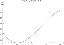
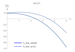
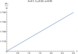
We see from the figure 14(a) and 14(c) that $\frac{dS_{T}}{dt}$ remains positive for all positive values of $\alpha$ and $\Gamma_{1}$. It is to be noted that we have taken energy transfer constant to be 0.1 i.e., greater than -0.001, keeping parity with constraint obtained from eqn. (60). On the other hand, from figure 14(b) it is observed that for a specific range of $\Gamma_{0}$, depending on the value of the interaction parameter $\alpha$, $\frac{dS_{T}}{dt}$ remains positive. To be specific we see that when $\Gamma_{0}<\alpha+3$ i.e., when $\alpha>\Gamma_{0}-3$, we see that $\frac{dS_{T}}{dt}$ remains positive. Therefore the validity of GSLT constrained mainly by the value of $\Gamma_{0}$, interaction parameter $\alpha$, and the energy transfer constant $A$.

VII Summary and Conclusion

In this work, we have studied the cosmological consequences of a particle creation mechanism from different perspectives for a particular form of particle creation rate $\Gamma=\Gamma_{0}H+\Gamma_{1}H^{-1}$ in an interacting two-fluid model in a spatially flat FRW universe. Here we have considered the creation of dark matter only, and energy flow from dark energy to dark matter due to interaction. We have considered the interaction term $Q=\alpha H\rho_{m}$ and calculated the analytic expressions of dark fluid energy densities $\rho_{m}$ and $\rho_{d}$ given by Eqn. (19) and Eqn. (20), following which we have obtained the analytic expression of the Hubble parameter given in Eqn. (21). Then we performed $\chi^{2}$ data analyses with combined data of Supernova-Ia (580 point), and Hubble data (27 point). We found the best fit values of the model parameters. It is also found that the present model is compatible with current observed data though it is not better than $\Lambda$CDM model. Further, the DE EoS parameter is estimated to be $\omega_{d}=-1.11$, i.e., it crossed the phantom divide line. Also, we observed that the estimated value of the interaction term is minimal, and there is no central difference between the estimated values of the model parameters in interacting and non-interacting cases. That is, from the statistical analysis viewpoint, the interaction has no significant effect on the model. Another exciting observation realized from the contour plots is that in the creation rate, one parameter, namely, $\Gamma_{1}$ can not influence any other parameters. At the same time, $\Gamma_{0}$ is linearly or nonlinearly related to other model parameters. Therefore, creation rate $\propto H$ plays a more crucial role in the evolution dynamics of the Universe than the term, which is inversely proportional to the Hubble parameter. We performed another analysis to understand the connection between the model paremeters and evolution dynamics more deeply.

In statefinder diagnostic analysis for distinct values of the model parameters $\alpha$, $\Gamma_{0}$, and $\Gamma_{1}$, different evolutionary trajectories have been achieved, which clearly show the dependency of the evolutionary trajectories on the model parameters in the $s-r$ plane. The distance of the present value $(s_{0},r_{0})$ from the $\Lambda CDM$ fixed point $(s=0,r=1)$ becomes shorter for smaller values of interaction parameter $\alpha$, and for larger values of $\Gamma_{0}$, $\Gamma_{1}$ in phantom era where all the evolutionary trajectories passed through the $\Lambda CDM$ fixed point at the early time. But in cosmological constant era, the distance of the present value $(s_{0},r_{0})$ from the $\Lambda CDM$ fixed point becomes shorter for larger values of $\alpha$ and for smaller values of $\Gamma_{0}$, $\Gamma_{1}$ whereas all the evolutionary trajectories end at the $\Lambda CDM$ fixed point in future. Similarly, in the quintessence era, the distance of the present value $(s_{0},r_{0})$ from the $\Lambda CDM$ fixed point becomes shorter for larger values of $\alpha$ and for smaller values of $\Gamma_{0}$, $\Gamma_{1}$ instead, the evolutionary trajectories never evolve through the $\Lambda CDM$ fixed point. Therefore the particle creation mechanism in a two dark fluid model can mimic the standard $\Lambda CDM$ fixed point at the early time in phantom era and in the future in cosmological constant era.

We also performed the statefinder diagnostic in the $q-r$ plane for this model where different evolutionary trajectories have been attained for various choices of the model parameters $\alpha$, $\Gamma_{0}$, and $\Gamma_{1}$. It clearly shows the dependency of evolutionary trajectories in the $q-r$ plane on the model parameters. In the phantom era as well as in the quintessence era, the evolutionary trajectories never evolve through the $de~{}Sitter$ fixed point $(q=-1,r=1)$. But in cosmological constant era, the distance of the present value $(q_{0},r_{0})$ from the $de~{}Sitter$ fixed point becomes shorter for larger values of $\alpha$ and for smaller values of $\Gamma_{0}$, $\Gamma_{1}$ whereas all the evolutionary trajectories end at the $de~{}Sitter$ fixed point in the future. So the model mimics the $de~{}Sitter$ fixed point in the future during the cosmological constant era.

From the dynamical study of the model, we obtain some interesting cosmological scenarios in the late times. A normally hyperbolic set of critical points $A$ represents the late-time accelerated Universe evolving in the phantom regime and entirely dominated by phantom fluid for ($y_{c}<-1$). It also represents dust dominated decelerated intermediate phase of the universe for $y_{c}=0$ when DE behaves as dust. Another normally hyperbolic set, $C$, represents the late-time scaling attractor in the phase space. For the parameter boundary $\alpha<\Gamma_{0}-3$, $C$ representing the accelerating universe in phantom regime (see fig. 11) and solving the coincidence problem. On the other hand, the normally hyperbolic set of points $D$ has interesting nature for $\alpha>\Gamma_{0}-3$ with $\Gamma_{1}\neq 0$, and it exhibits the late-time accelerated universe evolving in the cosmological constant era with the ratio of energy densities for DE and DM being unity, and as a result, it solves the coincidence problem (see figures (11) and 11). The authors in [102] showed that the scaling attractor cannot alleviate the coincidence problem when particle creation was taken as $\Gamma=\Gamma_{0}H$. Therefore, one can say that the model can predict the late-time accelerated evolutionary scheme of the Universe connected through a matter-dominated decelerated phase, and after fine tuning the initial conditions, we see that the ultimate fate of the universe is evolving in the cosmological constant era or in the phantom phase see fig. (13).

Finally, we carried out a thermodynamic analysis of the current model. As there are temperature difference between the system and horizon and also between the fluid components of the universe, thermal equilibrium can not hold, and therefore, non-equilibrium thermodynamic treatment is considered. Using Euler’s equation, we have calculated temperature evolution of the individual components DE and DM and finally calculated time derivative of the total entropy. As we have considered non-equilibrium thermodynamics, two extra terms corresponding to energy transfer between DE and DM within the universe and between the universe and the horizon, respectively, have been considered in the expression of total entropy. It is shown that if we use the best fit values of the model parameters obtained in statistical analysis, the generalized second law of thermodynamics is satisfied if the energy transfer constants are more significant than a particular value -0.001. Also, graphically, it has been shown that the validity of GSLT is crucially dependent on the $\Gamma_{0}$. In particular, when the energy transfer constant is greater than -0.001, GSLT is satisfied only when $\Gamma_{0}<\alpha+3$ i.e., when $\alpha>\Gamma_{0}-3$

From the overall analysis obtained from different sections, we conjecture that the evolution dynamics of the Universe are deeply connected with the particle creation rate and the interaction term. On a special note it is observed that $\Gamma_{0}$ plays a crucial role over $\Gamma_{1}$ in particle creation rate $\Gamma=\Gamma_{0}H+\frac{\Gamma_{1}}{H}$. Also, when $\alpha>\Gamma_{0}-3$, the results obtained from statefinder diagnosis, dynamical system analysis, and thermodynamic analysis also agree with current observed data. From this point of view, we need to do more research on this particular restriction on the model parameters. However, it may be then concluded that our present cosmological model with particle creation mechanism solves the coincidence problem and explains late time acceleration of the Universe and also satisfies the generalized second law of thermodynamics. Also, it can be predicted that the universe will eventually evolve in the cosmological constant era.

References

- [1] A. G. Riess et al., New Hubble Space Telescope Discoveries of Type Ia Supernovae at : Narrowing Constraints on the Early Behavior of Dark Energy, Astrophys. J. 659 (2007), 98-121.
- [2] Hawkins E et al, Mon. Not. Roy. Astron. Soc. 346 (2003), 78.
- [3] Tegmark M et al, Phys. Rev. D 69 (2006), 103501.
- [4] Cole S et al, Mon. Not. Roy. Astron. Soc. 362 (2005), 505.
- [5] Bennet C.L. et al, Astrophys. J. Suppl. 148 (2003), 1.
- [6] Komatsu E., Smith K.M, Dunkley J. et al., Astrophys. J. Supp. 192(2011), 18.
- [7] Perlmutter S., Aldering G., Goldhaber G. et al., Astrophys. J. 517(1999), 565.
- [8] Percival W.J., Reid B.A., Eisenstein D.J. et al., Mon. Not. R. Astron.Soc. 401(2010), 2148.
- [9] Sharov G.S., Vorontsova E.G., JCAP 1410(2014), 057. https://doi.org/10.1088/1475-7516/2014/10/057. arXiv:1407.5405 [gr-qc].
- [10] C. Wetterich, The cosmon model for an asymptotically vanishing time-dependent cosmological constant, Astron. Astrophys. 301 (1995) 321 [arXiv:hep-th/9408025].
- [11] L. Amendola, Coupled Quintessence, Phys. Rev. D 62 (2000) 043511 [arXiv:astro-ph/9908023].
- [12] D. Tocchini-Valentini and L. Amendola, Stationary dark energy with a baryon dominated era: Solving the coincidence problem with a linear coupling, Phys. Rev. D 65 (2002) 063508 [astro-ph/0108143].
- [13] L. Amendola and C. Quercellini, Tracking and coupled dark energy as seen by WMAP, Phys. Rev. D 68 (2003) 023514 [arXiv:astro-ph/0303228].
- [14] S. del Campo, R. Herrera and D. Pav´on, Toward a solution of the coincidence problem, Phys. Rev. D 78 (2008) 021302 [arXiv:0806.2116 [astro-ph]].
- [15] S. del Campo, R. Herrera and D. Pav´on, Interacting models may be key to solve the cosmic coincidence problem, J. Cosmol. Astropart. Phys. 0901 (2009) 020 [arXiv:0812.2210 [gr-qc]].
- [16] Wang,B., Zang,J., Lin,C. Y., Abdalla,E., Michelelti,S., Nucl.Phys.B 778 (2007), 69.
- [17] B.Wang,Y.G.Gong,E.Abdalla,Phys.Lett.B 624(2005), 141.
- [18] E. Di Valentino, A. Melchiorri, O. Mena, Can interacting dark energy solve the tension ?, Phys. Rev. D 96 (2017) 043503 [doi:10.1103/PhysRevD.96.043503].
- [19] S. Kumar and R. C. Nunes, Echo of interactions in the dark sector, Phys. Rev. D 96 (2017) 103511 [doi:10.1103/PhysRevD.96.103511].
- [20] W. Yang, A. Mukherjee, E. Di Valentino, and S. Pan, Interacting dark energy with time varying equation of state and the tension, Phys. Rev. D 98 (2018) 123527 [doi:10.1103/PhysRevD.98.123527].
- [21] S. Pan, W. Yang, C. Singha, and E. N. Saridakis, Observational constraints on sign-changeable interaction models and alleviation of the tension, Phys. Rev. D 100 (2019) 083539 [doi:10.1103/PhysRevD.100.083539].
- [22] E. Di Valentino, A. Melchiorri, O. Mena, S. Vagnozzid, Interacting dark energy in the early 2020s: A promising solution to the and cosmic shear tensions, Physics of the Dark Universe 30 (2020) 100666 [doi:10.1016/j.dark.2020.100666].
- [23] M. Lucca and D. C. Hooper, Shedding light on dark matter-dark energy interactions, Phys. Rev. D 102 (2020) 123502 [doi:10.1103/PhysRevD.102.123502].
- [24] S. Kumar, Remedy of some cosmological tensions via effective phantom-like behavior of interacting vacuum energy, Physics of the Dark Universe 33 (2021) 100862 [doi:10.1016/j.dark.2021.100862].
- [25] E. Di Valentino, O. Mena, S. Pan, L. Visinelli, W. Yang, A. Melchiorri, D. F. Mota, A. G. Riess, J. Silk, In the Realm of the Hubble tension-a Review of Solutions, Class. Quantum Grav. 38 (2021) 153001 [ doi:10.1088/1361-6382/ac086d ].
- [26] L. A. Anchordoqui, E. Di Valentino, S. Pan, W. Yang, Dissecting the H0 and S8 tensions with Planck + BAO + supernova type Ia in multi-parameter cosmologies, Physics of the Dark Universe, 32 (2021) 28 [doi:10.1016/j.jheap.2021.08.001 ].
- [27] F. Renzi, N. B. Hogg, W. Giarè, The resilience of the Etherington-Hubble relation, Monthly Notices of the Royal Astronomical Society 513 (2022) 4004–4014 [ https://doi.org/10.1093/mnras/stac1030].
- [28] Ö. Akarsu, S. Kumar, E. Özülker, and J. A. Vazquez, Relaxing cosmological tensions with a sign switching cosmological constant, Phys. Rev. D 104 (2021) 123512 [doi:10.1103/PhysRevD.104.123512].
- [29] A. Theodoropoulos, L. Perivolaropoulos, The Hubble Tension, The Crisis of Late Time Deformation Models and the Reconstruction of Quintessence Lagrangians, Universe 7 (2021) 300 [doi:10.3390/universe7080300].
- [30] S. Vagnozzi, New physics in light of the tension: An alternative view, Phys. Rev. D 102 (2020) 023518. (arXiv:1907.07569 [astro-ph.CO]).
- [31] L. Visinelli, S. Vagnozzi, U. Danielsson, Revisiting a Negative Cosmological Constant from Low-Redshift Data, Symmetry 11 (2019) 1035. (arXiv:1907.07953 [astro-ph.CO]).
- [32] E. Di Valentino, A. Melchiorri, O. Mena and S. Vagnozzi, Nonminimal dark sector physics and cosmological tensions, Phys. Rev. D 101 (2020) 063502. (arXiv:1910.09853 [astro-ph.CO]).
- [33] G. Cheng, Yin-Zhe Ma, F. Wu, J. Zhang, X. Chen, Testing interacting dark matter and dark energy model with cosmological data, Phys. Rev. D 102 (2020) 043517. (arXiv:1911.04520 [astro-ph.CO]).
- [34] S. Vagnozzi, L. Visinelli, O. Mena and D. F. Mota, Do we have any hope of detecting scattering between dark energy and baryons through cosmology?, Mon. Not. Roy. Astron. Soc. 493 (2020) 1139. (arXiv:1911.12374 [gr-qc]).
- [35] S. Pan, W. Yang and A. Paliathanasis, Nonlinear interacting cosmological models after Planck 2018 legacy release and the H0 tension, Mon. Not. Roy. Astron. Soc. 493 (2020) 3114. (arXiv:2002.03408 [astro-ph.CO]).
- [36] W. Yang, S. Pan, E. Di Valentino, O. Mena and A. Melchiorri, 2021- Odyssey: Closed, Phantom and Interacting Dark Energy Cosmologies, JCAP 10 (2021) 008. (arXiv:2101.03129 [astro-ph.CO]).
- [37] Li-Yang Gao, Ze-Wei Zhao, She-Sheng Xue and Xin Zhang, Relieving the tension with a new interacting dark energy model, JCAP 07 (2021) 005. (arXiv:2101.10714 [astro-ph.CO]).
- [38] M. Lucca, Dark energy-dark matter interactions as a solution to the tension, (arXiv:2105.09249 [astro-ph.CO]).
- [39] R. C. Nunes and E. Di Valentino, Dark sector interaction and the supernova absolute magnitude tension, Phys. Rev. D 104 (2021) 063529. (arXiv:2107.09151 [astro-ph.CO]).
- [40] Rui-Yun Guo, Lu Feng, Tian-Ying Yao and Xing-Yu Chen, Exploration of interacting dynamical dark energy model with interaction term including the equation-of-state parameter: alleviation of the tension, JCAP 12 (2021) 036. (arXiv:2110.02536 [gr-qc]).
- [41] A. Spurio Mancini and A. Pourtsidou, KiDS-1000 Cosmology: machine learning – accelerated constraints on Interacting Dark Energy with COSMOPOWER, Mon. Not. Roy. Astron. Soc. 512 (2022) L44. (arXiv:2110.07587 [astro-ph.CO]).
- [42] F. Ferlito, S. Vagnozzi, D. F. Mota and M. Baldi, Cosmological direct detection of dark energy: non-linear structure formation signatures of dark energy scattering with visible matter, Mon. Not. Roy. Astron. Soc. 512 (2022) 1885. (arXiv:2201.04528 [astro-ph.CO]).
- [43] R. C Nunes, S. Vagnozzi, S. Kumar, E. Di Valentino and O. Mena, New tests of dark sector interactions from the full-shape galaxy power spectrum, Phys. Rev. D 105 (2022) 123506. (arXiv:2203.08093 [astro-ph.CO]).
- [44] S. Pan, W. Yang, E. Di Valentino, D. F. Mota and J. Silk, IWDM: The fate of an interacting non-cold dark matter-vacuum scenario, arXiv:2211.11047 [astro-ph.CO].
- [45] Planck Collaboration (N. Aghanim et al.), Astron. Astrophys. 641 (2020) A6 [ doi:10.1051/0004-6361/201833910].
- [46] A. Pourtsidou and T. Tram, Reconciling CMB and structure growth measurements with dark energy interactions, Phys. Rev. D 94 (2016) 043518 [doi:10.1103/PhysRevD.94.043518].
- [47] Rui An et al., Relieving the tension between weak lensing and cosmic microwave background with interacting dark matter and dark energy models, JCAP 02 (2018) 038 [doi:10.1088/1475- 7516/2018/02/038].
- [48] S. Kumar, R. C. Nunes, S. Kumar Yadav,Dark sector interaction: a remedy of the tensions between CMB and LSS data, Eur. Phys. J. C 79 (2019) 576 [doi:10.1140/epjc/s10052-019-7087-7].
- [49] J.C.N. de Araujo, A. De Felice, S. Kumar, and R. C. Nunes, Minimal theory of massive gravity in the light of CMB data and the tension,Phys. Rev. D 104 (2021) 104057 [doi:10.1103/PhysRevD.104.104057].
- [50] F. Avila, A. Bernui, R. C Nunes, E. de Carvalho, C. P Novaes, The homogeneity scale and the growth rate of cosmic structures Get access Arrow, Monthly Notices of the Royal Astronomical Society 509(2) (2022) 2994–3003 [ https://doi.org/10.1093/mnras/stab3122].
- [51] Di Valentino et al., Cosmology intertwined III: and , Astroparticle Physics, 131 (2021) 102604 [https://doi.org/10.1016/j.astropartphys.2021.102604].
- [52] S. Pan and S. Chakraborty, A cosmographic analysis of holographic dark energy models, Int. J. Mod. Phys. D 23 (2014) 1450092 [doi:10.1142/S0218271814500928].
- [53] A. Bonilla and J. E. Castillo, Constraints on Dark Energy Models from Galaxy Clusters and Gravitational Lensing Data, Universe 4 (2018) 21 [https://doi.org/10.3390/universe4010021].
- [54] A. Bonilla Rivera and J. Enrique García-Farieta, Exploring the dark universe: Constraints on dynamical dark energy models from CMB, BAO and growth rate measurements, Int. J. Mod. Phys. D 28 (2019) 1950118 [https://doi.org/10.1142/S0218271819501189].
- [55] Y. L. Bolotin, A. Kostenko, O. A. Lemets and D. A. Yerokhin, Cosmological Evolution With Interaction Between Dark Energy And Dark Matter, Int. J. Mod. Phys. D 24 (2015) no.03, 1530007 [arXiv: 1310.0085] [astro-ph.CO].
- [56] B. Wang, E. Abdalla, F. Atrio-Barandela and D. Pavon, Dark Matter and Dark Energy Interactions: Theoretical Challenges, Cosmological Implications and Observational Signatures, Rept. Prog. Phys. 79 (2016) no.9, 096901 [arXiv:1603.08299] [astro-ph.CO].
- [57] Erickson J.K., Caldwell R., Steinhardt P.J., Armendariz-Picon C., Mukhanov V.F., Phys. Rev. Lett. 88(2002), 121301. https://doi.org/10.1103/PhysRevLett.88.121301.
- [58] Armendariz-Picon C., Mukhanov V., Steinhardt P.J., Phys. Rev. D 63(10)(2001), 103510.
- [59] A. Kamenschick, U. Moschella, V. Pasquier, Phys. Lett. B. 511 (2001), 265.
- [60] M. C. Bento, O. Bertolami, and A. A. Sen, Phys. Rev. D. 66 (2002), 043507.
- [61] B.Pourhassan, EO. Kahya, Results in Physics 4 (2014), 101.
- [62] Z.-K. Guo, Y.-Z. Zhang, Phys. Lett. B. 645 (2007), 326.
- [63] J.C. Fabris, S.V.B. Goncalves, P.E. de Souza, Gen. Relativ. Gravit. 34(2002), 53-63.
- [64] Lazkoz,R. et al, Physics of the Dark Universe 24 (2019), 100279.
- [65] Capozziello, S., and M. Francaviglia, Gen. Rel. Grav. 40(2008), 357.
- [66] Nojiri S., and S. D. Odintsov, Int. J. Geom. Meth.Mod. Phys. 4(2007), 115.
- [67] Bergmann, P. G., Int. J. Theor. Phys. 1(1968), 25.
- [68] Maartens R. Living Rev. Relativity, 7(2004), 7.
- [69] Schrdinger E., Physica (Amsterdam)6(1939), 899.
- [70] Parker L., Phys. Rev. Lett. 21(1968), 562.
- [71] Ford L.H., Parker L., Phys. Rev. D 16(1977), 245.
- [72] Zeldovich Y. B., Starobinsky A. A., Sov. Phys. JETP 34(1972), 1159.
- [73] Parker L., Phys. Rev. 183(1969), 1057.
- [74] Parker L., Phys. Rev. D 7(1973), 976.
- [75] Fulling S. A., Aspects of Quantum Field Theory in Curved Spacetime, Cambridge University Press, Cambridge (1989).
- [76] Yu. V. Pavlov, Grav. Cosmol. 14(2008), 314.
- [77] Grib A. A., Mamayev S. G. and Mostepanenko V. M., Vaccum Quantum effects in Strong Fields, Friedmann Laboratory Publishing, St. Petesburg (1994).
- [78] Prigogine I., Geheniau J., Gunzig E. and Nardone P., Gen. Relativ. Grav. 21(1989), 767.
- [79] Pan S., Barrow J .D, and Paliathanasis A., Eur. Phys. J. C 79(2019), 115.
- [80] V. Sahni, T. D. Saini, A. A. Starobinsky, U. Alam, Statefinder – a new geometrical diagnostic of dark energy, JETP Lett. 77 (2003),201. (Pisma Zh. Eksp. Teor. Fiz. 77 (2003), 249) (arXiv:astro-ph/0201498).
- [81] U. Alam, V. Sahni, T.D. Saini, A.A. Starobinsky, Exploring the Expanding Universe and Dark Energy using the Statefinder Diagnostic, Mon. Not. R. Astron. Soc. 344 (2003), 1057 (arXiv:astro-ph/0303009).
- [82] W. Zimdahl , D. Pavón, Statefinder Parameters for Interacting Dark Energy, Gen. Relativ. Gravit. 36 (2004), 1483.
- [83] X. Zhang, Statefinder diagnostic for coupled quintessence, Phys. Lett. B 611 (2005a), 1.
- [84] B. Chang et al, Statefinder parameters for interacting phantom energy with dark matter, JCAP 01 (2007), 016.
- [85] Y. Shao, Y. Gui, Statefinder Parameters for Tachyon Dark Energy Model, Mod. Phys. Lett. A 23 (2008), 65.
- [86] M. Malekjani, R. Zarei, M. Honari-Jafarpour, Holographic dark energy with time varying parameter , Astrophys Space Sci 343 (2013), 799.
- [87] X. Zhang, Statefinder diagnostic for holographic dark energy model, Int. J. Mod. Phys. D 14 (2005b), 1597.
- [88] J. Zhang, X. Zhang, H. Liu, Statefinder diagnosis for the interacting model of holographic dark energy, Physics Letters B 659 (2008), 26.
- [89] M. R. Setare, J. Zhang and X. Zhang, Statefinder diagnosis in a non-flat universe and the holographic model of dark energy, J. Cosmol. Astropart. Phys. 0703 (2007), 007.
- [90] L. Zhang, J. Cui, J. Zhang, and X. Zhang, Interacting model of new agegraphic dark energy: Cosmological evolution and statefinder diagnostic, Int. J. Mod. Phys. D 19 (2010), 21.
- [91] A. Khodam-Mohammadi, M. Malekjani, Cosmic behavior, statefinder diagnostic and analysis for interacting new agegraphic dark energy model in non-flat universe, Astrophys. Space Sci. 331 (2010), 265.
- [92] H. Wei, R.G. Cai, Statefinder diagnostic and analysis for the agegraphic dark energy models without and with interaction, Phys. Lett. B 655 (2007), 1.
- [93] M. Malekjani and A. Khodam-Mohammadi, Agegraphic Dark Energy Model in Non-Flat Universe: Statefinder Diagnostic and Analysis, Int. J. Mod. Phys. D 19 (2010), 1857.
- [94] M. Jamil · U. Debnath, FRW Cosmology with Variable and , Int. J. Theor. Phys. 50 (2011), 1602.
- [95] M. R. Setare, M. Jami, Statefinder diagnostic and stability of modified gravity consistent with holographic and agegraphic dark energy, Gen. Relativ. Gravit. 43 (2011), 293.
- [96] U. Debnath · M. Jamil, Correspondence between DBI-essence and modified Chaplygin gas and the generalized second law of thermodynamics, Astrophys. Space Sci. 335 (2011), 545.
- [97] J. K. Singh, Ritika Nagpal, S. K. J. Pacif, Statefinder diagnostic for modified Chaplygin gas cosmology in f(R,T) gravity with particle creation, nternational Journal of Geometric Methods in Modern Physics 15 (2018), 1850049.
- [98] G. Mandal, S. Chakraborty, S. Mishra, S. Kr. Biswas, A study of interacting scalar field model from the perspective of the dynamical systems theory, Physics of the Dark Universe 40 (2023), 101210.
- [99] G. Mandal and S. Kr. Biswas, Dynamical stability of an interacting quintessence with varying-mass dark matter particles in Lyra manifold, International Journal of Modern Physics D 31 (2022), 2250059.
- [100] G. Mandal, S. Kr. Biswas, S. Saha, A. Al Mamon, Dynamical system analysis of logotropic dark fluid with a power law in the rest-mass energy density, Physics of the Dark Universe 35 (2022), 100970.
- [101] S. Bahamonde, C. G. Boehmer, S. Carloni, E. J. Copeland, W. Fang and N. Tamanini, Phys. Rep. 775 (2018), 1 (arXiv:1712.03107 [gr-qc]).
- [102] S. Kr. Biswas, W. Khyllep, J. Dutta, and S. Chakraborty, Dynamical analysis of an interacting dark energy model in the framework of a particle creation mechanism, Phys. Rev. D 95 (2017), 103009.
- [103] S. Kr. Biswas and A. Biswas, Phase Space Analysis and Thermodynamics of Interacting Umami Chaplygin Gas in FRW Universe, The European Physical Journal C 81 (2021), 356.
- [104] Bardeen J. M., Canter B., Hawking S. W., Commun. Math. Phys. 31(1973), 161.
- [105] Hawking S. W., Commun. Math. Phys. 43 (1975), 199.
- [106] Bekenstein J. D., Phys. Rev. D 9(1974), 3292.
- [107] Saha S., Biswas A., Chakraborty S., Astrophys. Space Sc. 356 (2015) 141.
- [108] Callen H.,Thermodynamics (J.Wiley,1960).
- [109] Pavn D., Zimdahl W., Phys. Lett. B 628 (2005), 206.
- [110] Suzuki N., et al., Astrophys. J. 746 (2012) 85.
- [111] Cao S.-L., Li S., Yu H.-R. and Zhang T.-J., RAA (Research in Astronomy and Astrophysics) 18 (2018) 26.
- [112] Zhang C. et al., RAA (Research in Astronomy and Astrophysics) 14 (2014) 1221.
- [113] Shi K., Huang Y. F. and Lu T., Mon. Not. R. Astron. Soc. 426(2012), 2452–2462.