Bounding the joint numerical range of Pauli strings by graph parameters

Abstract

The interplay between the quantum state space and a specific set of measurements can be effectively captured by examining the set of jointly attainable expectation values. This set is commonly referred to as the (convex) joint numerical range. In this work, we explore geometric properties of this construct for measurements represented by tensor products of Pauli observables, also known as Pauli strings. The structure of pairwise commutation and anticommutation relations among a set of Pauli strings determines a graph $G$, sometimes also called the frustration graph. We investigate the connection between the parameters of this graph and the structure of minimal ellipsoids encompassing the joint numerical range. Such an outer approximation can be very practical since ellipsoids can be handled analytically even in high dimensions.

We find counterexamples to a conjecture from [C. de Gois, K. Hansenne and O. Gühne, arXiv:2207.02197], and answer an open question in [M. B. Hastings and R. O’Donnell, Proc. STOC 2022, pp. 776–789], which implies a new graph parameter that we call $\beta(G)$. Besides, we develop this approach in different directions, such as comparison with graph-theoretic approaches in other fields, applications in quantum information theory, numerical methods, properties of the new graph parameter, etc. Our approach suggests many open questions that we discuss briefly at the end.

I Introduction

Pauli strings, sets of Pauli operators acting on multiple qubits, are undeniably among the most essential and omnipresent objects in the field of quantum information theory. Besides their role as unitary transformations, they commonly serve as a fundamental building block for constructing observables. Examples for such constructed observables are widespread, spanning from virtually every Hamiltonian that is considered in the field of quantum computing [1, 2, 3, 4, 5], typical measurements in quantum communication protocols [6, 7, 8, 9], to the rich theory of spin systems in condensed matter physics [10, 11, 12, 13, 14, 15, 16].

A pivotal object of investigation in this context is the set of jointly attainable expectation values. For a given a set of $n$ Pauli strings $\mathcal{S}=\{S_{1},\dots,S_{n}\}$ acting on the Hilbert space $\mathcal{H}$, we will consider

$$J(\mathcal{S})=\left\{\left(\langle S_{1}\rangle_{\rho},\dots,\langle S_{n}\rangle_{\rho}\right)|\rho\in\mathcal{D}(\mathcal{H})\right\},$$ (1)

which is a convex compact subset of $\mathbb{R}^{n}$ (see Fig. 1 for examples); here and subsequently, $\mathcal{D}(\mathcal{H})$ denotes the set of all states on the Hilbert space ${\cal H}$, i.e. density matrices that are positive semidefinite and of unit trace.

For a general sequence ${\cal S}$ of observables, $J(\mathcal{S})$ in Eq. (1) is commonly referred to as (convex) joint numerical range [17], or convex support. For special sets of observables, this set may have however more specific names depending on the context. The most prominent example of this surely is the well-known Bloch ball/sphere, which can be understood as the joint numerical range of the three Pauli operators acting on a single qubit, i.e. $\mathcal{S}=\{X,Y,Z\}$.

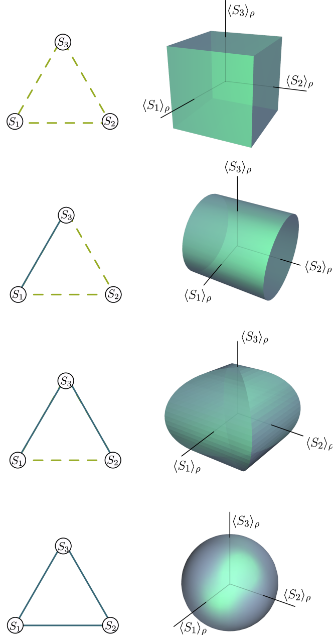
Figure 1: Joint numerical ranges of three Pauli strings whose commutation and anticommutation relations are represented by the 4 possible graphs of three vertices. The real lines represent the anticommutation relations and the dashed lines stand for commutativity relations.

For a more complex set of strings, the geometry of $J(\mathcal{S})$ is no longer necessarily captured by a sphere. Nevertheless, one can still ask for the smallest radius of a sphere or more generally an ellipsoid encompassing it. From a bare geometric perspective, this is the question tackled in this work.

The joint numerical range geometrically encodes a lot of relevant information about the interplay between observables and quantum states. Most strikingly, Hamiltonians that can be written as linear combinations of elements in ${\cal S}$ can be directly understood as linear functionals acting on $J(\mathcal{S})$. Correspondingly, the quest of finding ground-state energies and properties of states attaining them can be cast as the characterization of tangential hyperplanes on $J(\mathcal{S})$. Moreover, upper and lower bounds to ground-state energies correspond to inner and outer approximations of $J(\mathcal{S})$.

This insight, however, directly reveals that the precise characterization of the joint numerical range can, even for simple objects like Pauli strings, be an intrinsically hard problem, i.e. at least as hard as solving ground state problems on multiple qubits. This clearly justifies the demand for practical approximation techniques.

For the ground state problem itself, there is a humongous toolbox of known methods. Most of them provide inner bounds by reducing the optimization to a suitable variational class of states. Prominent examples to mention here are classical methods building on matrix product states [18, 19, 16], as well as implementations on quantum computers where algorithms like the Quantum Approximate Optimization Algorithm (QAOA) [20, 21, 22] or the Variational Quantum Eigensolver (VQE) [23, 24] are very popular.

Methods for outer approximations are however rather rare. In contrast to variational methods, handling of global structures is needed, which is typically much harder to achieve. Nevertheless, they can be from central importance. On one hand, outer bounds give complements for inner approximations, and by this an interval for the overall accuracy of an approximation attempt. On the other, the existence of a bound that can not be surpassed by any quantum state, also including those that are not in a variational class, can be critical in applications like cryptography or entanglement detection.

Notable examples for outer approximations can be found in [25, 26, 27]. Here the ansatz is to exploit the algebraic structure of the problem for setting up hierarchies of non-commutative polynomial relaxations [28, 29]. Even though, the scope of these methods is to solve a particular ground state problem, the feasible set of such a relaxation, sometimes called the relaxation to the quantum set, can be seen as an outer approximation to the joint numerical range $J(\mathcal{S})$. On the theoretical side, those methods usually come with a convergence guarantee. In practice, they however tend to show a very bad scaling behavior and typically saturate any practical limit of computational resources very quickly.

In the present work, we make steps towards a (semi-) analytical understanding of $J(\mathcal{S})$. For an $m$-dimensional ellipsoid $\mathcal{E}_{r}(w)$ with principal axes of length $r\cdot w_{i}$, where $w=(w_{1},\dots,w_{m})$ is a positive weight vector, we ask for the smallest $r\geq 0$ such that

$$J(\mathcal{S})\subseteq\mathcal{E}_{r}(w)$$ (2)

holds. Such a minimal ellipsoid, or at least an upper bound on $r$, then allows to compute bounds on ground-state energies analytically. This is especially interesting when we deal with high-dimensional objects, i.e. for long Pauli strings where the Hilbert space dimension scales exponentially. We have to clarify that the deployment of a new numerical toolbox is however not the scope of the present work, we will leave this for a future publication. Here, our main interest is to develop the foundations for a comprehensive understanding of the presented structures.

Finding a valid $r$, the optimal value of which we will refer to as (generalized) radius, corresponds to the non-linear optimization

$$r^{2}\geq\sup_{\rho}\sum w_{i}\langle S_{i}\rangle_{\rho}^{2}$$ (3)

Formally, this can be seen as an instance of so-called spectrahedral inclusion problems [30, 31], for which there are unfortunately no out-of-the-box solutions. Hence a lot of the particular structure of the present problem has to be leveraged in the solution.

The structure of minimal ellipsoids, as well as the structure of $J(\mathcal{S})$ itself (see Fig. 1), is closely connected to a graph $G$ that encodes the commutation and anticommutation relations within the strings of a set $\mathcal{S}$. This graph is also known under the names “frustration graph” [12, 11], “anticommutation graph” [32] or “anticompatibility graph” [33] in the literature. It can be shown [34, 25] (see Proposition 3 here) that the minimal radius of an ellipsoid is lower bounded by the weighted independence number of $G$ and upper bounded by its weighted Lovász number. Despite being efficiently computable, the Lovász number as an upper bound is known to be generally not tight [25, 34]. The tightness of the lower bound was however outstanding. For the spheroidal case $w=(1,1,\dots)$ it was conjectured [34], and extensively discussed during the coffee breaks of some workshops, that the independence number of $G$ describes the minimal radius. We show by an explicit example that this conjecture is false.

As a consequence, we introduce the minimal radius of an ellipsoid as a new graph parameter $\beta(G,w)$ and embark on its exploration. We develop a number of equivalent formulations of it, we show that it is monotonic non-increasing when passing to an induced subgraph, multiplicative under the so-called lexicographic product, etc. We calculate it for cyclic graphs $C_{n}$ and develop numerical tools to evaluate it for the complements of odd cycles $\overline{C}_{2n+1}$ supporting our conjecture that $\beta(\overline{C}_{2n+1})>2$ for all $n\geq 3$. At last, we also elaborate on the connection of our results to the quest for uncertainty relations between Pauli strings as their structure also depends directly on the structure of minimal ellipsoids[34, 35].

Since our results are closely related to multiple topics in quantum theory, graph theory and algebra analysis, the present results might provide new insights in those fields as well.

II Operator representations of graphs, graph parameters and main results

In order to get a leverage on minimal ellipsoids we have to find global structures of the problem that can be efficiently used. Regarding a set $\mathcal{S}$ of Pauli strings as the representation of an algebra is along those lines. Before we get there, it is however helpful to introduce the frustration graph and consider an example.

It is easy to see from the elementary properties of the four Pauli matrices (from now on including the identity), that each possible pair of Pauli strings either commutes or anticommutes. For a set of strings, this information can be encoded in a graph $G$, where each vertex represents a string and an edge is drawn whenever two strings anticommute. We will refer to this graph as frustration graph. Basic examples are the graphs show in Fig. 1. E.g. consider the third graph from above. This example was build by taking strings

$$S_{1}=X\otimes Y\quad S_{2}=Z\otimes Y\text{ and }S_{3}=Z\otimes Z$$ (4)

The strings $S_{1}$ and $S_{3}$ commute, whereas the string $S_{2}$ anticommutes with both of them. The joint numerical range is depicted next to it and arises from the intersection of two cylinders. For completeness, it makes sense to regard a cylinder as an asymptotic ellipsoid with one of its principal axes approaching infinity.

Note that, fixing a graph $G$ does not uniquely fix the set of strings representing it and there are more than only unitary degrees of freedom in between them. In this sense, there are more sets of strings than there are graphs. For example, any triple of strings will by construction give one of the graphs shown in Fig. 1.

For the questions considered in this work, we can however make a basic proposition, formulated with more detail in Theorem 16. It states that the radius of a minimal ellipsoid will be the same amongst all possible strings representing the same graph.

Proposition 1.

Let $\mathcal{S}_{1}$ and $\mathcal{S}_{2}$ be sets of Pauli strings with the same frustration graph. Then we have that for any ellipsoid with

$$\mathcal{E}_{r}(w)\supseteq J(\mathcal{S}_{1})\quad\text{ that }\quad\mathcal{E}_{r}(w)\supseteq J(\mathcal{S}_{2})$$ (5)

holds, and vice versa.

In other words, we can turn to investigate structures on a graph $G$ rather than on an explicit sets of strings. This can be done by introducing an algebraic framework. For a given graph $G$ we will consider operators with the abstract algebraic properties

• $S_{i}=S^{*}_{i}$,

• $S_{i}^{2}=\mathbb{I}$,

• $S_{i}^{2}\leq\mathbb{I}$,

• $\{S_{i},S_{j}\}=0$ if $i\sim j$,

• $[S_{i},S_{j}]=0$ $i\nsim j$,

where $i\sim j$ denotes vertices that are connected by an edge in a given graph $G$, i.e. $i$ and $j$ are adjacent.

It is clear that Pauli strings will obey all those properties. In order to investigate bounds on the radius of a minimal ellipsoid, we can however turn things around and consider all sets of operators fulfilling these conditions, or at least some of them. By this, we get a constructive tool for setting up relaxations of the joint numerical range. The detailed discussion of such operator representations of a graph will be the mathematical core of this work.

Definition 2.

For a given graph $G$, a set $\{S_{i}\}$ of operators on some Hilbert space $\mathcal{H}$ will be called

• a selfadjoint unitary representation for anticommutativity (SAURA) if (i), (ii), and (iii) hold. The set of all SAURAs will be denoted by $\mathcal{S}_{a}(G)$.

• a selfadjoint unitary representation (SAUR) if (i), (ii), (iii), and (iv) hold. The set of all SAURs will be denoted by $\mathcal{S}_{ac}(G)$.

• a selfadjoint representation for anticommutativity (SARA) if (i), (iia), and (iii) hold. The set of all SARAs will be denoted by $\mathcal{S}^{{\scriptscriptstyle\leq}}_{a}(G)$.

• a selfadjoint representation (SAR) if (i), (iia), (iii), and (iv) hold. The set of all SARs will be denoted by $\mathcal{S}^{{\scriptscriptstyle\leq}}_{ac}(G)$.

It is clear from the definition above that the different sets of graph representations include each other, i.e. every SAUR is a SAR and a SAURA, and they are all a SARA. This can be captured in the diagram

One can also consider the $C^{*}$-algebras generated by the different sets of relations. The algebra generated by all SAURs is known as quasi-Clifford algebra [36]. Each of these algebras naturally comes with a state space, too, and hence also with a joint numerical range. These joint numerical ranges are by construction outer approximations to the joint numerical range of an explicit set of Pauli strings. It is a finite-dimensional algebra and can be seen as a generalization of the Clifford algebra in the sense that we obtain the Clifford algebras as the sub-cases with a fully connected graph. The representation theory of this object has been worked out in [37, 36], a brief summary can be found in [25]. In a nutshell, we have that the Pauli strings with which we started are exactly generators of representations of this algebra. Bounds on minimal ellipsoids derived for this algebra are optimal. Bounds arising from considering the other algebras give relaxations, i.e. upper bounds on the radius.

The algebra corresponding to all SAURAs can generally be infinite-dimensional, yet still separable. As we will show later (Lemma 32), the algebra corresponding to SAR can be understood as tensor product of the quasi-Clifford algebra of the SAURs with a classical (i.e. commuting) algebra. An according result for the algebra corresponding to SAURA does however not hold.

For a set $\Omega$ of operator representations of a graph, where each representation $\mathcal{S}$ acts on a Hilbert space $\mathcal{H}_{\mathcal{S}}$, we can extend the notion of a joint numerical range by considering

$$\mathcal{J}\left(\Omega\right):=\left\{\left(\left\langle S_{i}\right\rangle_{\rho}\right)\ |\ \mathcal{S}=\{S_{i}\}\in\Omega,\rho\in\mathcal{D}(\mathcal{H}_{\mathcal{S}})\right\},$$ (6)

which is still a subset of $\mathbb{R}^{n}$, but now containing all possible tuples of expectations attainable by the set of operators corresponding to a particular operator representation. In order to analyze ellipsoids, it makes sense to also consider the set of squared expectations

$$\mathcal{Q}\left(\Omega\right):=\left\{\left(\left\langle S_{i}\right\rangle^{2}_{\rho}\right)\ |\ \mathcal{S}=\{S_{i}\}\in\Omega,\rho\in\mathcal{D}(\mathcal{H}_{\mathcal{S}})\right\}.$$ (7)

Given this set, the minimal radius of an ellipsoid [recall (3)] corresponding to some $w$ is the maximal value of a linear functional

$$\mathit{q}\left(\Omega,w\right):=\sup_{(v_{i})\in\mathcal{Q}\left(\Omega\right)}\sum_{i}w_{i}v_{i}.$$ (8)

In the spheroidal case, when all elements of $w$ are just $1$, we omit $w$ in the notation and write $\mathit{q}\left(\Omega\right)$. Further, we denote by $\overline{\mathcal{Q}}\left(\Omega\right)$ the convex hull of $\mathcal{Q}\left(\Omega\right)$.

For $\Omega$ a $\mathcal{S}_{ac}(G),\mathcal{S}^{{\scriptscriptstyle\leq}}_{ac}(G),\mathcal{S}_{a}(G)$ or $\mathcal{S}^{{\scriptscriptstyle\leq}}_{a}(G)$, it holds that

$$\mathcal{J}\left(\Omega\right)=\{(\pm\sqrt{q_{i}})|(q_{i})\in\mathcal{Q}\left(\Omega\right)\},$$ (9)

since $\{\pm S_{i}\}\in\Omega$ if $\{S_{i}\}\in\Omega$. In this case, the characterization of $\mathcal{J}\left(\Omega\right)$ is equivalent to the one of $\mathcal{Q}\left(\Omega\right)$. We remark that $\mathcal{J}\left(\Omega\right)$ is always convex and contains what is called the stable set polytope $\operatorname{STAB}(G)$ that, in those four cases, is given by

$$\operatorname{STAB}(G)=\{(v_{i})\mid v_{i}v_{j}=0\text{ if }i\sim j,v_{i},v_{j}\in\{0,1\}\}.$$

Eq. (8) basically states that the full structure of ellipsoids encompassing the different $\mathcal{J}\left(\Omega\right)$, and by this also any $J(\mathcal{S})$ of interest, is encoded in the convex hulls of the different $\mathcal{Q}\left(\Omega\right)$. Their interrelation, which is worked out in the following sections, can be captured by the following proposition.

Proposition 3.

(Main results) Let $G$ be a graph. Let $\operatorname{STAB}(G)$ be its stable set polytope and let $\operatorname{TH}(G)$ be its Lovász-theta body. For $\mathcal{Q}$ evaluated on different representations of $G$, as introduced above, we have the following ordering relations:

$$\operatorname{STAB}(G)\,\overset{{\color[rgb]{0.58984375,0.66796875,0.1953125}(a)}}{\subseteq}\,\begin{matrix}\overline{\mathcal{Q}}\left(\mathcal{S}_{ac}(G)\right)\\ \rotatebox[origin={c}]{90.0}{$=$}_{{\color[rgb]{0.58984375,0.66796875,0.1953125}(b)}}\\ \overline{\mathcal{Q}}\left(\mathcal{S}^{{\scriptscriptstyle\leq}}_{ac}(G)\right)\end{matrix}\,\overset{{\color[rgb]{0.58984375,0.66796875,0.1953125}(c)}}{\subseteq}\,\begin{matrix}\mathcal{Q}\left(\mathcal{S}_{a}(G)\right)\\ \rotatebox[origin={c}]{90.0}{$=$}_{{\color[rgb]{0.58984375,0.66796875,0.1953125}(d)}}\\ \mathcal{Q}\left(\mathcal{S}^{{\scriptscriptstyle\leq}}_{a}(G)\right)\end{matrix}\overset{{\color[rgb]{0.58984375,0.66796875,0.1953125}(e)}}{=}\,\operatorname{TH}(G)$$ (10)

with the Lovász theta body defined as

$$\operatorname{TH}(G)=\{|\langle v_{0}|v_{i}\rangle|^{2}\mid\langle v_{i}|v_{i}\rangle=1,\langle v_{i}|v_{j}\rangle=0\text{ if }i\sim j\}.$$

The equality of $\mathcal{Q}\left(\mathcal{S}_{ac}(G)\right)$ and $\mathcal{Q}\left(\mathcal{S}^{{\scriptscriptstyle\leq}}_{ac}(G)\right)$ (b), as well as that of $\mathcal{Q}\left(\mathcal{S}_{a}(G)\right)$ and $\mathcal{Q}\left(\mathcal{S}^{{\scriptscriptstyle\leq}}_{a}(G)\right)$ (d), are outlined in Sec. VI. Hence, we can focus the main part of our investigations to SAURA (Sec. III) and SAUR (Sec. IV).

Consequently, for any non-negative weight vector $w$,

$$\alpha(G,w)\,{\leq}\,\begin{matrix}\mathit{q}\left(\mathcal{S}_{ac}(G),w\right)\\ \rotatebox[origin={c}]{90.0}{$=$}\\ \mathit{q}\left(\mathcal{S}^{{\scriptscriptstyle\leq}}_{ac}(G),w\right)\end{matrix}\,{\leq}\,\begin{matrix}\mathit{q}\left(\mathcal{S}_{a}(G),w\right)\\ \rotatebox[origin={c}]{90.0}{$=$}\\ \mathit{q}\left(\mathcal{S}^{{\scriptscriptstyle\leq}}_{a}(G),w\right)\end{matrix}{=}\,\vartheta(G,w),$$ (11)

where $\alpha(G,w)\!=\!q(\operatorname{STAB}(G),w),\vartheta(G,w)\!=\!q(\operatorname{TH}(G),w)$ are the weighted independence number and Lovász number of $G$, and $\mathit{q}\left(\mathcal{S}_{ac}(G),w\right)$ is denoted as $\beta(G,w)$ later.

Establishing a bridge to the Lovász-theta body $\operatorname{TH}(G)$ and the Lovász number is especially interesting from a numerical perspective since $\vartheta(G,w)$ can be computed via semi-definite programming (SDP). Using this as a tool for outer bounds is advantageous since the size of this SDP scales with $n$, i.e., the number of vertices of $G$, and by this ultimately with the number of strings in a set $\mathcal{S}$. This has to be put into contrast with the problem of computing ground-state energies, i.e. hyperplanes of $J(\mathcal{S})$, whose size scales with the Hilbert space dimension $2^{n}$, where $n$ is the length of the strings.

For $G$ a perfect graph, all the inequalities in (10) and (11) become equalities since $\operatorname{STAB}(G)=\operatorname{TH}(G)$. The nontrivial cases hide in imperfect graphs, where odd cycles and odd anticycles are basic ones. As it turns out, odd cycles can be characterized clearly and odd anticycles are rather more complicated and hence more interesting.

Here we have that

Theorem 4.

$\overline{\mathcal{Q}}\left(\mathcal{S}_{ac}(C_{n})\right)=\operatorname{STAB}(C_{n}),\forall n\in\mathbb{N}^{+}$.

and

Theorem 5.

$\operatorname{STAB}(\bar{C}_{n})\subsetneq\overline{\mathcal{Q}}\left(\mathcal{S}_{ac}(\bar{C}_{n})\right)\subsetneq\operatorname{TH}(\bar{C}_{n})$, especially, $\alpha(\bar{C}_{n})<\beta(\bar{C}_{n})<\vartheta(\bar{C}_{n})$ for $n=2k+1$ and $3\leq k\leq 10$.

Those two theorems might imply a new classification of imperfect graphs, which calls for more investigation in graph theory.

Furthermore, for a given set of observables $\{S_{i}\}$, there is a complete hierarchy of SDP relaxations for $\mathit{q}\left(\{S_{i}\}\right)$ as explained in Appendix A. Two practical see-saw methods for the numerical estimation are also supplemented in Appendix A. Finally, the estimation can be improved once we know the purity of the state.

III Selfadjoint unitary representation for anticommutativity

As introduced in Sec. II, for a given graph $G$, a set $\{S_{i}\}$ of selfadjoint unitaries is said to be a selfadjoint unitary representation for anticommutativity (SAURA) of $G$ if $i\sim j$ implies $\{S_{i},S_{j}\}=0$. An essential task is to characterize $\mathit{q}\left(\mathcal{S}_{a}(G)\right)$ and $\mathcal{Q}\left(\mathcal{S}_{a}(G)\right)$.

Lemma 6.

(Cf. [25]) For any graph $G$, it holds that

$$\alpha(G)\leq\mathit{q}\left(\mathcal{S}_{a}(G)\right)\leq\vartheta(G).$$ (12)

In fact, $\mathit{q}\left(\{S_{i}\}\right)\geq\alpha(G)$ for any SAUR $\{S_{i}\}$ of graph $G$, which can be proven directly by choosing the state $\rho$ as a common eigenstate of a set of the commuting observables from $S_{i}$, where $i$ ranges over an independent set of $G$. For any graph $G$, it holds that $\alpha(G)\leq\vartheta(G)$. In the case that $G$ is a perfect graph, we have $\alpha(G)=\vartheta(G)$ [38]. Hence, the upper bounds in Eq. (12) is tight for perfect graphs. Especially, in the case that $G$ is a clique graph with $n$ vertices where any two vertices are connected, the relation $\mathit{q}\left(\mathcal{S}_{a}(G)\right)=1$ holds. For a given set of observables, numerical estimation of $\mathit{q}\left(\{S_{i}\}\right)$ can in principle provide a more exact bound. Different numerical methods to estimate $\mathit{q}\left(\{S_{i}\}\right)$ are presented in Sec. A. Here we take the graph-theoretic approach, and provide an exact characterization of $\mathit{q}\left(\mathcal{S}_{a}(G)\right)$and $\mathcal{Q}\left(\mathcal{S}_{a}(G)\right)$.

Graph-theoretic approach has been explored extensively in quantum contextuality [39], where the orthogonality representation (OR) of a graph is used [40]. For a given graph with $n$ vertices, a set of unit vectors $\{|v_{i}\rangle\}_{i=1}^{n}$ is said to be an OR of the graph $G$ if $\langle v_{i}|v_{j}\rangle=0$ when $i\sim j$. An OR of a given graph implies an SAURA of the same graph.

Lemma 7.

For a given set of $d$-dimensional vectors $\{\langle v_{i}|=(v_{i1},\ldots,v_{id})\}$, denote $S_{i}=\sum_{k}v_{ik}A_{k}$ where $\{A_{k}\}_{k=1}^{d}$ is a set of anticommuting selfadjoint unitaries, it holds that $\{S_{i},S_{j}^{\dagger}\}/2=\langle v_{i}|v_{j}\rangle\mathbb{I}$.

We remark that there are indeed SAURA of a graph that cannot be constructed from an OR. For example, the operators $\{X\mathbb{I},Y\mathbb{I},Z\mathbb{I},ZZ\}$ and their anticommutativity graph. Indeed, those four operators are linearly independent, but there is no operator which anticommutes with all of them at the same time. Hence, there is no anticommuting basis for those four operators. In this sense, there are more SAURAs than ORs of a given graph. Nevertheless, such a construction of SAURAs from ORs is the key step in the following proof.

Theorem 8.

$\mathcal{Q}\left(\mathcal{S}_{a}(G)\right)=\operatorname{TH}(G)$ for any graph $G$.

Proof.

It is equivalent to prove that $\mathit{q}\left(\mathcal{S}_{a}(G),w\right)=\vartheta(G,w)$ for any non-negative weight vector $w$. Equation (12) includes already the result that $\mathit{q}\left(\mathcal{S}_{a}(G),w\right)\leq\vartheta(G,w)$ when all the elements of $w$ are just $1$. For the general non-negative weight vector $w$, we prove it later in Sec. VI.

To show that $\mathit{q}\left(\mathcal{S}_{a}(G),w\right)\geq\vartheta(G,w)$, we construct an exact $\{S_{i}\}\in\mathcal{S}_{a}(G)$ such that $\mathit{q}\left(\{S_{i}\},w\right)=\vartheta(G,w)$.

Denote $\{|v_{i}\rangle\}_{i=1}^{n}$ and $|u\rangle$ the OR of the graph $G$ and the state such that $\vartheta(G,w)=\sum_{i=1}^{n}w_{i}|\langle v_{i}|u\rangle|^{2}$, which can be assumed to be real without loss of generality. Denote $\{A_{i}\}_{i=1}^{r}$ a set of $d$-dimensional normalized traceless observables satisfying $\{A_{i},A_{j}\}/2=\delta_{ij}\mathbb{I}$, where $r$ is the dimension of $\{|v_{i}\rangle\}_{i=1}^{n}$. By setting $S_{i}=\sum_{k=1}^{r}v_{i,k}A_{k}$, the $S_{i}$’s are Hermitian and $\{S_{i},S_{j}\}/2=\langle v_{i}|v_{j}\rangle\mathbb{I}$, which implies that $\{S_{i}\}$ is an SAURA of $G$.

For a given state $\rho$, denote $\mathcal{M}_{\rho}$ the matrix whose $(i,j)$-th element is $\sqrt{w_{i}w_{j}}\left\langle\{S_{i},S_{j}\}/2\right\rangle_{\rho}$. In this special case, $\left\langle\{S_{i},S_{j}\}/2\right\rangle_{\rho}=\langle v_{i}|v_{j}\rangle$ which is independent of the exact state $\rho$. Then $\lambda_{\max}(\mathcal{M}_{\rho})=\vartheta(G,w)$. Denote $|a\rangle$ the eigenvector of $\mathcal{M}_{\rho}$ corresponding to the maximal eigenvalue, we have $\langle a|\mathcal{M}_{\rho}|a\rangle=\vartheta(G,w)$.

Denote by $|s\rangle$ the eigenstate of $\sum_{i}a_{i}\sqrt{w_{i}}S_{i}$ corresponding to the maximal eigenvalue and $\sigma=|s\rangle\langle s|$. Then

$$\sum_{i}w_{i}\left\langle S_{i}\right\rangle_{\sigma}^{2} \geq\left(\sum_{i}a_{i}\sqrt{w_{i}}\left\langle S_{i}\right\rangle_{\sigma}\right)^{2}$$

$$=\left(\left\langle\sum_{i}a_{i}\sqrt{w_{i}}S_{i}\right\rangle_{\sigma}\right)^{2}$$

$$=\left\langle\left(\sum_{i}a_{i}\sqrt{w_{i}}S_{i}\right)^{2}\right\rangle_{\sigma}$$

$$=\vartheta(G,w),$$ (13)

where the first line is from Cauchy-Schwarz inequality since $|a\rangle$ is normalized, the third line is by the definition of $\sigma$ and the last line is from the definition of $|a\rangle$ and the fact that $\mathcal{M}_{\rho}$ is independent of the state $\rho$. Finally, we have $\mathit{q}\left(\mathcal{S}_{a}(G),w\right)\geq\vartheta(G,w)$ and complete the proof. ∎

Thus, we have a new physical explanation of the graph parameter $\vartheta(G)$. We remark that the construction in Lemma 7 is crucial for the proof, as the last line in Eq. (III) may not hold for a general SAURA. For a given set of observables $\{S_{i}\}$, Eq. (III) implies another equivalent definition of $\mathit{q}\left(\{S_{i}\},w\right)$, that is

$$\mathit{q}\left(\{S_{i}\},w\right)=\max_{\rho,\ a\ s.t.\ ||a||_{2}=1}\Big{(}\sum_{i}a_{i}\sqrt{w_{i}}\left\langle S_{i}\right\rangle_{\rho}\Big{)}^{2}.$$ (14)

As shown in Appendix A, the new definition leads to a See-Saw method for the estimation of $\mathit{q}\left(\{S_{i}\},w\right)$.

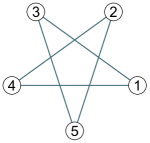
Figure 2: Pentagon graph $C_{5}$.

Example 9.

For the pentagon graph, its Lovász number can be achieved with the state $\langle u|=(1,0,0)$ and the following orthogonal representation $\{|v_{i}\rangle\}_{i=1}^{5}$, where

$$\langle v_{i}|=\left(\tau,\tau^{\prime}\cos(2\pi i/5),\tau^{\prime}\sin(2\pi i/5)\right),$$ (15)

and $\tau=(1/5)^{1/4},\tau^{\prime}=\sqrt{1-\tau^{2}}$.

Hence, by choosing

$$S_{i}=\sum_{k}v_{ik}\sigma_{k},\forall i=1,\ldots,5,$$ (16)

$$\rho=(\mathbb{I}+\sigma_{1})/2,$$ (17)

where $\sigma_{1}=X,\sigma_{2}=Y,\sigma_{3}=Z$ are Pauli matrices, then we have $\sum_{i}\left\langle S_{i}\right\rangle_{\rho}^{2}=\sqrt{5}$.

There is another concise proof of Theorem 8. In fact, $\left\langle S_{i}\right\rangle_{\rho}=x\langle v_{i}|u\rangle$ if we take $\rho=(\mathbb{I}+x\sum_{k}u_{k}A_{k})/d$, where $|x|\leq 1$. We note that $\rho\succeq 0$ is a legal state since the maximal eigenvalue of $\sum_{k}u_{k}A_{k}$ is no more than $1$. Thus, $\sum_{i}w_{i}\left\langle S_{i}\right\rangle_{\rho}^{2}=x^{2}\sum_{i}w_{i}(\langle v_{i}|u\rangle)^{2}=x^{2}\vartheta(G,w)$ by definition. By taking $x=\pm 1$, we complete the proof.

Along this direction, there are further results.

Tighter bound based on purity

Note that the purity $\operatorname{Tr}(\rho^{2})=(1+x^{2})/d$, which provides the intuition that the purity of the state could affect the joint expectation values. A direct observation is that $\sum_{i}\left\langle S_{i}\right\rangle^{2}=0$ always holds for the maximally mixed state. By making use of the information of purity, we can improve the estimation of joint expectation values.

Theorem 10.

For a given set of $d$-dimensional observables $\{S_{i}\}\in\mathcal{S}_{a}(G)$, and a state $\rho$, we have

$$\sum_{i}\left\langle S_{i}\right\rangle_{\rho}^{2}\leq\min\{[d\operatorname{Tr}(\rho^{2})-1]\vartheta(G),\vartheta(G)\}.$$ (18)

Furthermore, for any given graph $G$ and the purity of state, the upper bound in Eq. (18) is always tight.

The discussion at the beginning of this section works as a constructive proof. We remark that $[d\operatorname{Tr}(\rho^{2})-1]\vartheta(G)\leq\vartheta(G)$ always hold when the dimensional is $2$, like the case in Example 9. Notice that $\operatorname{Tr}(\rho^{2})$ is related to the linear entropy of the state, the inequality shows how the entropy of the state affects the joint expectation values. It is interesting to see that the linear entropy of the state affects the joint expectation values only when the linear entropy is large enough, i.e., when $\operatorname{Tr}(\rho^{2})\leq 2/d$. This happens when the temperature of the thermal state is high, or the system is highly entangled with the environment.

Relaxation of anticommutation relation

The anticommutation relation of operators leads to the orthogonality of them in the sense of trace product. That is, if $\{S_{i},S_{j}\}=0$, then $\operatorname{Tr}(S_{i}S_{j})=0$. However, the converse is not necessarily true, e.g., $S_{1}=XX$ and $S_{2}=ZZ$. For convenience, denote $|S\rangle$ as the vector obtained by flattening the operator $S$ row by row. With this notation, $\operatorname{Tr}(S_{i}S_{j})=\langle S_{i}|S_{j}\rangle$. As we will see later, $\{S_{i},S_{j}\}=0$ also implies $\operatorname{Tr}(S_{i})=\operatorname{Tr}(S_{j})=0$. Hence, $\left\langle S_{i}\right\rangle_{\rho}=\langle S_{i}|\tilde{\rho}\rangle$, where $\tilde{\rho}=\rho-\mathbb{I}/d$ and $d$ is the dimension. Notice that $\langle\tilde{\rho}|\tilde{\rho}\rangle=\operatorname{Tr}(\rho^{2})-1/d$, $\langle S_{i}|S_{i}\rangle=d$. By comparing with the definition of Lovász number, we have a generalization of Theorem 8.

Theorem 11.

For a given graph $G$ and its $d$-dimensional orthogonality representation with $\{S_{i}\}$ such that $\langle S_{i}|S_{i}\rangle=d$ and $\langle S_{i}|S_{j}\rangle=0$ if $i\sim j$, then

$$\sum_{i}\left\langle S_{i}\right\rangle_{\rho}^{2}\leq[d\operatorname{Tr}(\rho^{2})-1]\vartheta(G).$$ (19)

We have two remarks: first, the constructive proof of Theorem 8 implies that the bound in Theorem 11 is tight whenever $\operatorname{Tr}(\rho^{2})\leq 2/d$. Secondly, Lemma 7 and the vectorization of matrices, Theorem 8 and Theorem 11 give hints to the similarity of the role of $\vartheta(G)$ in quantum contextuality and joint expectation values.

IV Selfadjoint unitary representations

The set of operators, where any pair either commutes or anticommutes, plays an important role as exemplified by the Pauli strings. The commutation and anticommutation relations of such a set $\{S_{i}\}$ can be encoded into a so-called frustration graph $G$ [12, 11], where $i\sim j$ if $\{S_{i},S_{j}\}=0$, and $i\not\sim j$ if $[S_{i},S_{j}]=0$. By checking extensive examples, it is conjectured in Ref. [34] that

$$\mathit{q}\left(\{S_{i}\}\right)=\alpha(G).$$ (20)

Whether Eq. (20) can be violated is also an open question in Ref. [25]. Conversely, for a given graph $G$, we can consider its representation by a set $\{S_{i}\}$ of selfadjoint unitaries, in the sense that $\{S_{i},S_{j}\}=0$ if $i\sim j$ and $[S_{i},S_{j}]=0$ if $i\not\sim j$. This representation is called selfadjoint unitary representation (SAUR) [41]. By taking the graph-theoretic approach instead of starting from a special set, we denote $\beta(G,w)=\mathit{q}\left(\mathcal{S}_{ac}(G),w\right)$, where $\mathcal{S}_{ac}(G)$ is the set of all SAURs of $G$. The conjecture in Eq. (20) is equivalent to $\beta(G)=\alpha(G)$. In Ref. [25], no such an example is known that $\beta(G)>\alpha(G)$. To continue, we first introduce the standard SAUR of a given graph, which is defined deductively. The standard SAUR can help us to reduce the complexity of considerations, since we only need to focus on the standard SAUR to obtain $\beta(G)$ as we will see later.

Definition 12.

For a given graph $G$ and one of its edges $(i_{0},j_{0})$, other vertices except $i_{0}$ and $j_{0}$ can be devided into four groups $V_{0},V_{1},V_{2},V_{3}$, such that

• $i\not\sim i_{0}$ and $i\not\sim j_{0}$ for any $i\in V_{0}$;

• $i\not\sim i_{0}$ and $i\sim j_{0}$ for any $i\in V_{1}$;

• $i\sim i_{0}$ and $i\sim j_{0}$ for any $i\in V_{2}$;

• $i\sim i_{0}$ and $i\not\sim j_{0}$ for any $i\in V_{3}$.

The subgraph $G^{\prime}$ of $G$ with vertices in $\cup_{i=0}^{4}V_{i}$ is said to be a Pauli-$(i_{0},j_{0})$-induced subgraph of $G$ if

• when $i\in V_{k_{1}},j\in V_{k_{2}}$ where $k_{1}\neq k_{2}\in\{1,2,3\}$, we have $i\sim j$ (or $i\not\sim j$) in $G^{\prime}$ if and only if $i\not\sim j$ (or $i\sim j$) in $G$;

• otherwise, $i\sim j$ in $G^{\prime}$ if and only if $i\sim j$ in $G$.

Definition 13.

For a given graph $G$ and one of its edges $(i_{0},j_{0})$, denote $G^{\prime}$ the Pauli-$(i_{0},j_{0})$-induced subgraph of $G$, from a standard SAUR $\{S^{\prime}_{i}\}$ of $G^{\prime}$, we call the following SAUR a standard one of $G$:

$$\left(\bigcup_{k=0}^{3}\{\sigma_{k}\otimes S^{\prime}_{i}\}_{i\in V_{k}}\right)\cup\{X_{i_{0}}\otimes\mathbb{I},Z_{j_{0}}\otimes\mathbb{I}\}.$$ (21)

If $G$ has no edge, we assign $\mathbb{I}$ or $1$ to all its vertices.

If we take the pentagon $C_{5}$ in Fig. 2 as the original graph, and $(1,3)$ as the edge, then the Pauli-$(1,3)$-induced subgraph $G^{\prime}$ is a triangle. Continually, the Pauli-$(4,5)$-induced subgraph $G^{\prime\prime}$ of $G^{\prime}$ is just the vertex $2$. Hence, the standard SAURs $\{S^{\prime\prime}_{i}\},\{S^{\prime}_{i}\}$ and $\{S_{i}\}$ of $G^{\prime\prime},G^{\prime}$ and $G$, respectively, are

$$S^{\prime\prime}_{2}=1,S^{\prime}_{2}=Y,S^{\prime}_{4}=X,S^{\prime}_{5}=Z,$$ (22)

$$S_{1}=X\mathbb{I},S_{2}=\mathbb{I}Y,S_{3}=Z\mathbb{I},S_{4}=XX,S_{5}=ZZ,$$ (23)

where we have omitted the symbol of tensor product, and $X\mathbb{I}$ means $X\otimes\mathbb{I}$ etc.

Theorem 14 (Cf. [41]).

For a given graph $G$ and one SAUR $\{S_{i}\}$ of $G$, there is a unitary $U$ and standard SAUR $\{\bar{S}_{i}\}$ such that $US_{i}U^{\dagger}=\bar{S}_{i}\otimes D_{i}$, where $\{D_{i}\}$ is a set of commuting selfadjoint unitaries.

The standard SAUR is succinct, however, it loses the information of the symmetry in the graph. To reflect the structure of the graph, we introduce the edge SAUR.

Definition 15.

For a given graph $G$ with $n$ vertices and the edge set $E$, the set of selfadjoint operators $\{A_{i}\}_{i=1}^{n}$ with $A_{i}=\otimes_{e\in E}O_{e,i}$ is called the edge SAUR of $G$, where $O_{e,i}=X$ if $i$ is the start of $e$, and $O_{e,i}=Z$ if $i$ is the end of $e$, otherwise, $O_{e,i}=\mathbb{I}$.

For different SAURs of the same graph $G$, their joint expectation values are related.

Theorem 16.

For a given graph $G$, $\mathit{q}\left(\{S_{i}\}\right)=\mathit{q}\left(\{\bar{S}_{i}\}\right)$ where $\{S_{i}\}$ is a SAUR of $G$ and $\{\bar{S}_{i}\}$ is a standard one.

Proof.

From the convexity of $\sum_{i}\left\langle S_{i}\right\rangle^{2}$, we know that we only need to prove for the case that $\rho$ is a pure state $|\psi\rangle\langle\psi|$. Since $D_{i}$ commutes with each other, we can assume $D_{i}$’s are diagonal matrices. Denote $d_{2}$ the dimension of $D_{i}$’s, then we have the decomposition

$$U|\psi\rangle=\sum_{i=1}^{d_{2}}\sqrt{p_{i}}|\phi_{i}\rangle\otimes|i\rangle,$$ (24)

where $p_{i}\geq 0$ and $\sum_{i}p_{i}=1$.

Hence,

$$\left\langle S_{i}\right\rangle =\sum_{kl}\sqrt{p_{i}p_{j}}\langle\phi_{k}|\bar{S}_{i}|\phi_{l}\rangle\langle k|D_{i}|l\rangle$$

$$=\sum_{k}p_{k}\langle\phi_{k}|s_{ik}\bar{S}_{i}|\phi_{k}\rangle,$$ (25)

where $s_{ik}\in\{-1,1\}$ is the $k$-th diagonal element in $D_{i}$.

Then we have

$$\left\langle S_{i}\right\rangle^{2}=\left(\sum_{k}p_{k}\langle\phi_{k}|s_{ik}\bar{S}_{i}|\phi_{k}\rangle\right)^{2}\leq\sum_{k}p_{k}\langle\phi_{k}|\bar{S}_{i}|\phi_{k}\rangle^{2},$$ (26)

which implies that

$$\sum_{i}\left\langle S_{i}\right\rangle^{2} \leq\sum_{k}p_{k}\left(\sum_{i}|\langle\phi_{k}|\bar{S}_{i}|\phi_{k}\rangle|^{2}\right)$$

$$\leq\max_{k}\sum_{i}\langle\phi_{k}|\bar{S}_{i}|\phi_{k}\rangle^{2}.$$ (27)

Thus, $\mathit{q}\left(\{S_{i}\}\right)\leq\mathit{q}\left(\{\bar{S}_{i}\}\right)$.

On the other hand, denote $|\phi\rangle$ the optimal state for $\mathit{q}\left(\{\bar{S}_{i}\}\right)$ and $|\psi_{0}\rangle$ the common eigenstate for $D_{i}$’s, then

$$\sum_{i}\left\langle S_{i}\right\rangle^{2}_{\rho}=\sum_{i}\langle\phi|\bar{S}_{i}|\phi\rangle^{2},$$ (28)

where $\rho=|\psi\rangle\langle\psi|$ and $|\psi\rangle=U^{\dagger}[|\phi\rangle\otimes|\psi_{0}\rangle]$. Thus, we have $\mathit{q}\left(\{S_{i}\}\right)\geq\mathit{q}\left(\{\bar{S}_{i}\}\right)$. This finishes the proof. ∎

Hence, we have $\beta(G)=\mathit{q}\left(\{\bar{S}_{i}\}\right)$ where $\{\bar{S}_{i}\}$ is any standard SAUR of $G$. A similar result of Theorem 16 for the weighted version can be proven in the same way. Consequently, $\mathcal{Q}\left(\mathcal{S}_{ac}(G)\right)=\mathcal{Q}\left(\{{S}_{i}\}\right)$ where $\{{S}_{i}\}$ is any SAUR of $G$. However, $\mathcal{J}\left(\mathcal{S}_{ac}(G)\right)$ might be strictly larger than $\mathcal{J}\left(\{S_{i}\}\right)$ due to the sign of each expectation value. To recover the whole set of $\mathcal{J}\left(\mathcal{S}_{ac}(G)\right)$, it is enough to consider the complete SAUR as defined below.

Definition 17.

For a given graph $G$ with $n$ vertices and its standard SAUR $\{\bar{S}_{i}\}$, the set $\{S_{i}\}$ consisting of

$$S_{i}=\bar{S}_{i}\otimes\Big{(}\bigotimes_{k=1}^{n}Z^{\delta_{ik}}\Big{)}$$ (29)

is said to be a complete SAUR, where $\delta_{ik}=1$ if $i=k$, otherwise, $\delta_{ik}=0$.

As we can see, the auxiliary part $\{\otimes_{k=1}^{n}Z^{\delta_{ik}}\}$ can recover all signs in $\{-1,1\}^{\otimes n}$. Effectively, this provides a cover of $\mathcal{J}\left(\mathcal{S}_{ac}(G)\right)$ with multiple copies of $\mathcal{J}\left(\{\bar{S}_{i}\}\right)$.

V The beta parameter

For the characterization of the graph parameter $\beta(G)$, we consider some properties of it in this section. First, we show that $\beta(G)$ is indeed a parameter different from $\alpha(G)$, although for certain graphs it can occur that $\alpha(G)=\beta(G)$.

Corollary 18.

For the graph $G_{10}$ and $C_{5}$ in Fig. 3,

$$\beta(G_{10})=\alpha(G_{10})=\beta(C_{5})=\alpha(C_{5})=2.$$ (30)

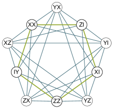
Figure 3: A graph $G_{10}$ with $10$ vertices and one of its standard realizations, which contains a pentagon $C_{5}$ as an induced subgraph (green, thick).

Proof.

Notice that $\beta(G)\geq\alpha(G)$, $\beta(G_{10})\geq\beta(C_{5})$ and $\alpha(G_{10})=\alpha(C_{5})=2$, we only need to prove $\beta(G_{10})=2$. According to Theorem 16, it is sufficient to consider the standard SAUR of $G_{10}$ as the one in Fig. 3 and denote it by $\{S_{i}\}_{i=1}^{10}$.

Because of the convexity of $\sum_{i}\left\langle S_{i}\right\rangle_{\rho}^{2}$ in terms of state $\rho$, we only need to consider the state to be a pure $4$-dimensional state

$$|\psi\rangle=\{ \cos\theta_{1},e^{it_{1}}\sin\theta_{1}\cos\theta_{2},e^{it_{2}}\sin\theta_{1}\sin\theta_{2}\cos\theta_{3},$$

$$e^{it_{3}}\sin\theta_{1}\sin\theta_{2}\sin\theta_{3}\}.$$ (31)

A direct calculation shows that

$$\sum_{i=1}^{10}\left\langle S_{i}\right\rangle^{2}=2.$$ (32)

∎

The fact that $\beta(C_{5})=2$ has also been proven in Ref. [25] in another approach. We have two remarks: first, for any $4$-dimensional pure state, Eq. (32) is equivalent to

$$\left\langle\mathbb{I}X\right\rangle^{2}+\left\langle\mathbb{I}Z\right\rangle^{2}+\left\langle XY\right\rangle^{2}+\left\langle YY\right\rangle^{2}+\left\langle ZY\right\rangle^{2}=1.$$ (33)

By permuting $X,Y,Z$ and the parties, we can obtain other equalities. Secondly, the standard SAUR of $G_{10}$ cannot be generated by the construction in Lemma 7, since there is no operator anticommuting with $X\mathbb{I},Y\mathbb{I},Z\mathbb{I}$ at the same time, meanwhile, the dimension of the linear span of all the operators in this standard SAUR is $10$.

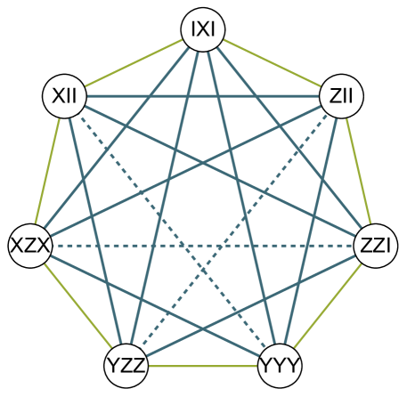
Figure 4: Graph of the counterexample and its SAUR. A pair of observables anticommute when the corresponding vertices are connected by an edge in the graph of an anti-heptagon $\bar{C}_{7}$ (blue, thick) and commute when connected by an edge in the graph of a heptagon $C_{7}$ (green, thin). The subgraph of $\bar{C}_{7}$ (blue, real, thick) is named as $G_{7}$.

However, the conjecture in Eq. (20) is not true generally. A simple counterexample is the anti-heptagon and its standard SAUR as shown in Fig. 4. To be more explicit, the seven operators are

$$S_{1} =ZZ\mathbb{I}, S_{2} =Z\mathbb{I}\mathbb{I}, S_{3} =\mathbb{I}X\mathbb{I}, S_{4} =X\mathbb{I}\mathbb{I},$$

$$S_{5} =XZX, S_{6} =YZZ, S_{7} =YYY.$$ (34)

It can be checked by hand that these operators form one standard SAUR of $\bar{C}_{7}$, and $\alpha(\bar{C}_{7})=2$.

Let $\rho=|v\rangle\langle v|$ be the state that corresponds to the largest eigenvector of $\sum_{i}S_{i}$. With a little bit more hand work, or by using a computer algebra system, one can check that

$$\sum\langle S_{i}\rangle_{\rho}^{2}=(9+4\sqrt{2})/7\approx 2.09384>2=\alpha(\bar{C}_{7}),$$ (35)

which disproves the conjecture in Eq. (20). Besides, $\vartheta(\bar{C}_{7})=1+1/\cos(\pi/7)\approx 2.10992$. Thus, in general, $\alpha(G)\leq\beta(G)\leq\vartheta(G)$ are indeed three different graph parameters.

Then we consider properties of the beta number under graph operations, e.g., the addition, graph products like lexicographic product and XOR product. Those properties are helpful for the estimation of the $\beta(G)$ for large graph $G$, which might be impossible with the numerical methods.

Theorem 19.

For a given graph $G$ which can be divided into two subgraphs $G_{1},G_{2}$ where all vertices in $G_{1}$ are connected with all vertices in $G_{2}$, then $\beta(G)=\max\{\beta(G_{1}),\beta(G_{2})\}$.

Proof.

For a given SAUR of $G$, we label the operators for $G_{1}$ as $\{A_{i}\}$, the ones for $G_{2}$ as $\{B_{j}\}$.

On the one hand, for any state $\rho$ (for convenience, we omit the state $\rho$ in the mean value), we have

$$\sum_{i}\left\langle A_{i}\right\rangle^{2}+\sum_{j}\left\langle B_{j}\right\rangle^{2}$$

$$= \max_{x,y}\left[\left\langle\sum_{i}x_{i}A_{i}\right\rangle^{2}+\left\langle\sum_{j}y_{j}B_{j}\right\rangle^{2}\right]$$

$$= \max_{x,y,t}\left[\left\langle t_{1}\sum_{i}x_{i}A_{i}+t_{2}\sum_{j}y_{j}B_{j}\right\rangle^{2}\right]$$

$$\leq \max_{x,y,t}\left\langle\left(t_{1}\sum_{i}x_{i}A_{i}+t_{2}\sum_{j}y_{j}B_{j}\right)^{2}\right\rangle,$$ (36)

where $x,y,t$ are unit real vectors.

By definition of $\{A_{i}\}$ and $\{B_{j}\}$, we have

$$\max_{x,y,t}\left\langle\left(t_{1}\sum_{i}x_{i}A_{i}+t_{2}\sum_{j}y_{j}B_{j}\right)^{2}\right\rangle$$

$$= \max_{x,y,t}\left[t_{1}^{2}\left\langle\left(\sum_{i}x_{i}A_{i}\right)^{2}\right\rangle+t_{2}^{2}\left\langle\left(\sum_{j}y_{j}B_{j}\right)^{2}\right\rangle\right]$$

$$= \max_{x,y,t}\max\left\{\left\langle\left(\sum_{i}x_{i}A_{i}\right)^{2}\right\rangle,\left\langle\left(\sum_{j}y_{j}B_{j}\right)^{2}\right\rangle\right\}$$

$$\leq \max_{x,y,t}\max\{\beta(G_{1}),\beta(G_{2})\}$$

$$= \max\{\beta(G_{1}),\beta(G_{2})\},$$ (37)

By definition,

$$\beta(G) =\max_{\rho,\{A_{i}\},\{B_{j}\}}\left[\sum_{i}\left\langle A_{i}\right\rangle^{2}_{\rho}+\sum_{j}\left\langle B_{j}\right\rangle^{2}_{\rho}\right],$$ (38)

which implies that $\beta(G)\leq\max\{\beta(G_{1}),\beta(G_{2})\}$.

On the other, $\beta(G)\geq\max\{\beta(G_{1}),\beta(G_{2})\}$, which completes the proof. ∎

Corollary 20.

If we add one new vertex to a graph $G$ and result in a graph $G^{\prime}$ in the way that the new vertex is connected to all vertices in $G$, then $\beta(G^{\prime})=\beta(G)$.

Theorem 21.

For a given graph $G$ which can be divided into two subgraphs $G_{1},G_{2}$ where any vertex in $G_{1}$ is disconnected with any vertex in $G_{2}$, $\beta(G)=\beta(G_{1})+\beta(G_{2})$.

Proof.

Without loss of generality, we assume that the state $\rho$ and the SAUR $\{A_{i}\}$ result in $\beta(G_{1})$, and the state $\sigma$ and the SAUR $\{B_{j}\}$ result in $\beta(G_{2})$. Then $\{A_{i}\otimes\mathbb{I}_{B}\}\cup\{\mathbb{I}_{A}\otimes B_{j}\}$ is a SAUR of $G$. Direct calculation shows that

$$\sum_{i}\!\left\langle A_{i}\!\otimes\!\mathbb{I}\right\rangle_{\rho\otimes\sigma}^{2}\!+\!\sum_{j}\left\langle\mathbb{I}\otimes B_{j}\right\rangle_{\rho\otimes\sigma}^{2}\!=\!\beta(G_{1})\!+\!\beta(G_{2}).$$ (39)

Besides, for any SAUR $\{\tilde{A}_{i}\}\cup\{\tilde{B}_{j}\}$ of $G$ and any state $\tau$, we have

$$\sum_{i}\left\langle\tilde{A}_{i}\right\rangle_{\tau}^{2}+\sum_{j}\left\langle\tilde{B}_{j}\right\rangle_{\tau}^{2}$$

$$\leq \max_{\rho,\{A_{i}\}}\sum_{i}\left\langle A_{i}\right\rangle_{\rho}^{2}+\max_{\sigma,\{B_{j}\}}\sum_{j}\left\langle B_{j}\right\rangle_{\sigma}^{2}$$

$$= \beta(G_{1})+\beta(G_{2}).$$ (40)

In total, we have $\beta(G)=\beta(G_{1})+\beta(G_{2})$ by definition. ∎

For two given graphs $G_{1}$ and $G_{2}$, we denote by $G_{1}[G_{2}]$ their lexicographic product, whose vertex set is the Cartesian product of the graphs’ vertex sets and then $(i_{1},j_{1})\sim(i_{2},j_{2})$ if $i_{1}\sim i_{2}$, or $j_{1}\sim j_{2}$ when $i_{1}=i_{2}$.

Theorem 22.

For two given graphs $G_{1}$ and $G_{2}$, $\beta(G)$ is multiplicative under the lexicographic product: $\beta(G_{1}[G_{2}])=\beta(G_{1})\beta(G_{2})$.

Proof.

Denote $\{A_{ij}\}$ any SAUR of $G=G_{1}[G_{2}]$, where $A_{ij}$ represents the vertex in $G$ which corresponds to $i$ in $G_{1}$ and $j$ in $G_{2}$. Denote $\bar{A}_{i}=\sum_{j}x_{ij}A_{ij}/\lambda_{i}$, where $\{x_{ij}\}_{j}$ is the normalized vector of $\{\left\langle A_{ij}\right\rangle\}_{j}$, and $\lambda_{i}$ is the maximal eigenvalue of $\sum_{j}x_{ij}A_{ij}$. We remark that $\{\bar{A}_{i}\}\in\mathcal{S}^{{\scriptscriptstyle\leq}}_{ac}(G_{1})$, and $\{A_{ij}\}_{j}\in\mathcal{S}_{ac}(G_{2})$ for all $i$.

By definition,

$$\beta(G) =\max_{\rho,\{A_{ij}\}\in\mathcal{S}_{ac}(G)}\sum_{i}\sum_{j}\left\langle A_{ij}\right\rangle_{\rho}^{2}$$

$$=\max_{\rho,\{A_{ij}\}\in\mathcal{S}_{ac}(G)}\sum_{i}\left\langle\sum_{j}x_{ij}A_{ij}\right\rangle_{\rho}^{2}$$

$$=\max_{\rho,\{A_{ij}\}\in\mathcal{S}_{ac}(G)}\sum_{i}\lambda_{i}^{2}\left\langle\bar{A}_{i}\right\rangle_{\rho}^{2}$$

$$\leq\beta(G_{2})\max_{\rho,\{A_{i}\}\in\mathcal{S}^{{\scriptscriptstyle\leq}}_{ac}(G_{1})}\sum_{i}\left\langle A_{i}\right\rangle_{\rho}^{2}$$

$$=\beta(G_{2})\beta(G_{1}),$$ (41)

where the inequality in the fourth line is from the following fact:

$$\lambda_{i}^{2}=\max_{\rho}\left\langle\sum_{j}x_{ij}A_{ij}\right\rangle_{\rho}^{2}\leq\beta(G_{2}),$$ (42)

and the last equality is proven in Sec. VI.

On the other hand, without loss of generality, we assume that the state $\rho$ and the SAUR $\{A_{i}\}$ result in $\beta(G_{1})$, the state $\sigma$ and the SAUR $\{B_{j}\}$ result in $\beta(G_{2})$. Denote

$$A_{ij}=A_{i}\otimes\left[\bigotimes_{k\in G_{1}}B_{j}^{\delta_{ik}}\right],$$ (43)

where $\delta_{ik}=1$ if $k=i$, otherwise, $\delta_{ik}=0$. By construction, $\{A_{ij}\}\in\mathcal{S}(G)$. Let $\tau:=\rho\otimes\sigma^{\otimes n_{1}}$, where $n_{1}$ is the number of vertices in $G_{1}$. Then we have

$$\sum_{ij}\left\langle A_{ij}\right\rangle_{\tau}^{2}=\sum_{ij}\left\langle A_{i}\right\rangle_{\rho}^{2}\left\langle B_{j}\right\rangle_{\sigma}^{2}=\beta(G_{1})\beta(G_{2}),$$ (44)

concluding the proof. ∎

For any large graph with decomposition into small graphs with known beta numbers through the two addition operations and lexicographic product, its exact beta number can be obtained. For example, if we take the lexicographic product of five $\bar{C}_{7}$, that is, $G=\bar{C}_{7}^{[\ ]5}$, then $\beta(G)=\beta^{5}(\bar{C}_{7})\approx 40.2452$. However, $\alpha(G)=\alpha^{5}(\bar{C}_{7})=32$ and $\vartheta(G)=\vartheta^{5}(\bar{C}_{7})\approx 41.8144$ since those two parameters are also multiplicative under the lexicographic product [42, 43, 44]. Hence, the integer part of $\beta(G)$, $\alpha(G)$ and $\vartheta(G)$ can be all different. This closes the open question in Ref. [25] with the answer: there are indeed graphs with beta number strictly larger than the independence number, the gap between them can even be large.

The removal of one edge is also one basic graph operation, which can relate different graph products. One important property shared by the independence number and the Lovász number is that they do not decrease under the edge-removal. However, this does not hold for the beta number. Here we take $\bar{C}_{7}$ and its subgraph $G_{7}$ (see Fig. 4) as an example.

Theorem 23.

$\beta(G_{7})=2<\beta(\bar{C}_{7})$.

Proof.

Notice that $G_{7}$ is isomorphic to an induced subgraph of $C_{5}[K_{2}]$, where $K_{2}$ is just one edge. Thus,

$$\beta(G_{7})\leq\beta(C_{5})\beta(K_{2})=2.$$ (45)

On the other hand, $\beta(G_{7})\geq\alpha(G_{7})=2$, which completes the proof. ∎

Although the beta number is between the independence number and the Lovász number, its behavior under edge-removal is rather strange. Nevertheless, the beta number does not increase under the vertex-removal, same as the independence number and the Lovász number. More explicitly, $\beta(G^{\prime})\leq\beta(G)$ if $G^{\prime}$ is an induced subgraph of $G$.

Tensor product of systems is used in quantum mechanics often. Denote $G$ the anticommutativity and commutativity graph corresponding to the tensor product of the SAURs of $G_{1}$ and $G_{2}$. We can directly verify that $G$ is the XOR product of $G_{1},G_{2}$, that is, $(i_{1},j_{1})\sim(i_{2},j_{2})$ if and only if only one of $i_{1}\sim i_{2}$ and $j_{1}\sim j_{2}$ holds. In this case, denote $G=G_{1}\times G_{2}$.

Theorem 24.

For two given graphs $G_{1}$ and $G_{2}$, $\beta(G_{1}\times G_{2})\geq\beta(G_{1})\beta(G_{2})$.

Proof.

Denote $\{A_{i}\}$ and $\{B_{j}\}$ the standard SAUR of $G_{1}$ and $G_{2}$, respectively. Then we know that

$$\mathit{q}\left(\{A_{i}\}\right)=\beta(G_{1}),\mathit{q}\left(\{B_{j}\}\right)=\beta(G_{2}).$$ (46)

Hence,

$$\beta(G_{1}\times G_{2}) \geq\mathit{q}\left(\{A_{i}\otimes B_{j}\}\right)$$

$$\geq\max_{\rho_{1}\otimes\rho_{2}}\sum_{ij}\left\langle A_{i}\otimes B_{j}\right\rangle_{\rho_{1}\otimes\rho_{2}}^{2}$$

$$=\beta(G_{1})\beta(G_{2}),$$ (47)

since $\{A_{i}\otimes B_{j}\}_{ij}$ is a SAUR of $G_{1}\times G_{2}$. ∎

For a perfect graph $G$, we know that $\alpha(G)=\vartheta(G)=\alpha^{\star}(G)$ which implies that $\alpha(G)=\beta(G)=\vartheta(G)=\alpha^{\star}(G)$. For imperfect graphs, odd cycles and odd anticycles are basic building blocks. To continue, we make the following claim:

Theorem 25.

$$\max_{\rho}\!\left[\left\langle\mathbb{I}Y\right\rangle_{\rho}^{2}\!+\!\left\langle XX\right\rangle_{\rho}^{2}\!+\!\left\langle ZZ\right\rangle_{\rho}^{2}\!-\!\left\langle YY\right\rangle_{\rho}^{2}\right]\!=\!1.$$ (48)

Proof.

It is enough to show that the maximum of the following SDP is $1$, as a relaxation of the original theorem:

$$l= \max_{\gamma}\operatorname{Tr}\left[\gamma W\right]$$

such that $$\operatorname{Tr}(A_{0}\gamma)=1,\gamma\succeq 0,$$

$$\operatorname{Tr}[A_{i}\gamma]\geq 0,i=1,2,3,$$ (49)

where $W=\mathbb{I}Y\mathbb{I}Y+XXXX+ZZZZ-YYYY$, $A_{0}=\mathbb{I}\mathbb{I}\mathbb{I}\mathbb{I}$, $A_{1}=XZXZ$, $A_{2}=Y\mathbb{I}Y\mathbb{I}$ and $A_{3}=ZXZX$.

Then the dual SDP is

$$l^{\prime}= \min y_{0}$$

such that $$\sum_{i=0}^{3}y_{i}A_{i}-{W}\succeq 0,$$

$$y_{i}\leq 0,i=1,2,3.$$ (50)

Since the case that $y_{0}=1$ and $y_{i}=-1$ for $i=1,2,3$ is a feasible solution, we know that $l\leq l^{\prime}\leq 1$. However, by taking $\rho=|\Psi^{+}\rangle\langle\Psi^{+}|$ with $|\Psi^{+}\rangle=(|00\rangle+|11\rangle)/\sqrt{2}$ in Eq. (48), we have $l\geq 1$. Consequently, $l=1$. ∎

We remark that it is already known that [45] $l=1$ if we only consider the state in the form $\rho=(\mathbb{I}+xXX+yYY+zZZ)/4$, for which $\left\langle\mathbb{I}Y\right\rangle_{\rho}=0$. Hence, our result generalizes the known one, which is considered often in quantum correlations like discord [45].

By considering the relation between the standard SAUR of different odd cycles, we have

Lemma 26.

$\beta(C_{2n+3})-\beta(C_{2n+1})\leq 1$.

Proof.

For convenience, we label the vertice of $C_{2k+1}$ in the way such that

$$1\sim 3\sim\cdots\sim 2k+1\sim 2(k-1)\sim\cdots\sim 2,$$ (51)

where $k=n,n+1$.

The proof is based on the observation that the standard SAUR $\{S^{\prime}_{i}\}_{i=1}^{2n+3}$ of $C_{2n+3}$ can be constructed as follows:

$$S^{\prime}_{i}=S_{i}\mathbb{I}_{2},\ \forall i=1,\ldots,2n,$$

$$S^{\prime}_{2n+1}=\mathbb{I}_{2^{n-1}}XX,S^{\prime}_{2n+2}=\mathbb{I}_{2^{n-1}}ZZ,$$

$$S^{\prime}_{2n+3}=\mathbb{I}_{2^{n}}Y,$$ (52)

where $\{S_{i}\}_{i=1}^{2n}\cup\{\mathbb{I}_{2^{n-1}}Y\}$ is the standard SAUR of $C_{2n+1}$.

Denote $S^{\prime\prime}_{2n+1}=\mathbb{I}_{2^{n-1}}YY$, we have

$$\beta(C_{2n+3})= \max_{\sigma^{\prime}}\left[\sum_{i=1}^{2n}\left\langle S^{\prime}_{i}\right\rangle_{\sigma^{\prime}}^{2}+\sum_{i=2n+1}^{2n+3}\left\langle S^{\prime}_{i}\right\rangle_{\sigma^{\prime}}^{2}\right]$$

$$= \max_{\sigma^{\prime}}\left[\left(\sum_{i=1}^{2n}\left\langle S^{\prime}_{i}\right\rangle_{\sigma^{\prime}}^{2}+\left\langle S^{\prime\prime}_{2n+1}\right\rangle_{\sigma^{\prime}}^{2}\right)+\right.$$

$$\left.\qquad\left(\sum_{i=2n+1}^{2n+3}\left\langle S^{\prime}_{i}\right\rangle_{\sigma^{\prime}}^{2}-\left\langle S^{\prime\prime}_{2n+1}\right\rangle_{\sigma^{\prime}}^{2}\right)\right]$$

$$\leq \beta(C_{2n+1})+1,$$ (53)

where the last inequality is from the fact that $\{S^{\prime}_{i}\}_{i=1}^{2n}\cup\{S^{\prime\prime}_{2n+1}\}$ is one SAUR of $C_{2n+1}$ and Theorem 25. ∎

Since $\alpha(C_{2n+1})=n$, $\beta(C_{5})=\alpha(C_{5})=2$, Theorem 25 and Lemma 26 lead to the following theorem.

Theorem 27.

$\overline{\mathcal{Q}}\left(\mathcal{S}_{ac}(C_{m})\right)=\operatorname{STAB}(C_{m})$.

Proof.

Since $C_{m}$ is a perfect graph when $m$ is an even number, the fact that $\operatorname{STAB}(C_{m})=\operatorname{TH}(C_{m})$ implies $\overline{\mathcal{Q}}\left(\mathcal{S}_{ac}(C_{m})\right)=\operatorname{STAB}(C_{m})$.

When $m=2n+1$ is an odd number, Theorem 25 and Lemma 26 result in the fact that $\beta(C_{2n+1})=\alpha(C_{2n+1})$. Consequently, this implies that $\overline{\mathcal{Q}}\left(\mathcal{S}_{ac}(C_{2n+1})\right)=\operatorname{STAB}(C_{2n+1})$, since the only nontrivial facet of $\operatorname{STAB}(C_{2n+1})$ has the norm vector $(1,\cdots,1)$ [46]. ∎

Numerically, we have $\vartheta(\bar{C}_{2n+1})>\beta(\bar{C}_{2n+1})>\alpha(\bar{C}_{2n+1})=2$ for $n\leq 10$, see Fig. 5 for more details; for any graph $G$ with no more than $9$ vertices, if $\beta(G)>\alpha(G)$, then $G$ has either $\bar{C}_{7}$ or $\bar{C}_{9}$ as an induced subgraph.

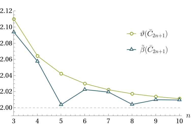
Figure 5: The estimation $\tilde{\beta}(\bar{C}_{2n+1})$ of $\beta(\bar{C}_{2n+1})$ in comparison with $\vartheta(\bar{C}_{2n+1})$. For each estimation, we have used the second See-Saw method with $500$ rounds of iteration.

These observations motivate the following conjectures.

Conjecture 28.

$\overline{\mathcal{Q}}\left(\mathcal{S}_{ac}(G)\right)=\operatorname{TH}(G)$ if and only if $G$ is perfect.

Conjecture 29.

$\overline{\mathcal{Q}}\left(\mathcal{S}_{ac}(G)\right)\supsetneq\operatorname{STAB}(G)$ if and only if $G$ has some $\bar{C}_{2n+1}$ as an induced subgraph where $n\geq 3$.

The second conjecture, which we dub “quasi-perfect graph conjecture”, is similar to the strong perfect graph theorem which states that $\operatorname{STAB}(G)\subsetneq\operatorname{TH}(G)$ if and only if $G$ is imperfect, i.e., $G$ has one $C_{2n+1}$ or $\bar{C}_{2n+1}$ as an induced subgraph where $n\geq 2$. We believe that “quasi-perfect graph conjecture” could have an important impact in graph theory if it holds.

VI Selfadjoint representations and return to joint numerical range beyond $\mathbf{\pm 1}$-observables

Whether in SAURA or in SAUR, we have only considered selfadjoint unitaries, which can limit the range of applications. We generalize our setting to non-unitary operators in this section.

Definition 30.

For a given graph $G$, a set of operators $\{A_{i}\}$ is said to be a selfadjoint representation for anticommutativity (SARA) of $G$ if each $A_{i}$ is selfadjoint, $\{A_{i},A_{j}\}=0$ when $i\sim j$. Furthermore, if $[A_{i},A_{j}]=0$ whenever $i\not\sim j$, $\{A_{i}\}$ is said to be a selfadjoint representation (SAR) of $G$.

For a given graph $G$, denote $\mathcal{S}^{{\scriptscriptstyle\leq}}_{a}(G)$ the set of all its SARAs, and $\mathcal{S}^{{\scriptscriptstyle\leq}}_{ac}(G)$ the set of all its SARs. By definition, $\mathcal{S}_{a}(G)\subseteq\mathcal{S}^{{\scriptscriptstyle\leq}}_{a}(G)$, and $\mathcal{S}_{ac}(G)\subseteq\mathcal{S}^{{\scriptscriptstyle\leq}}_{ac}(G)$. Surprisingly, maximizing over $\mathcal{S}^{{\scriptscriptstyle\leq}}_{a}(G)$ instead of $\mathcal{S}_{a}(G)$ does not result in a larger value, same for $\mathcal{S}^{{\scriptscriptstyle\leq}}_{ac}(G)$ and $\mathcal{S}_{ac}(G)$.

Theorem 31.

$\mathcal{Q}\left(\mathcal{S}^{{\scriptscriptstyle\leq}}_{a}(G)\right)=\mathcal{Q}\left(\mathcal{S}_{a}{G}\right)=\operatorname{TH}(G)$.

Proof.

Notice that $\operatorname{TH}(G)\subseteq\mathcal{Q}\left(\mathcal{S}_{a}(G)\right)\subseteq\mathcal{Q}\left(\mathcal{S}^{{\scriptscriptstyle\leq}}_{a}{G}\right)$. Hence, it is sufficient to prove $\mathcal{Q}\left(\mathcal{S}^{{\scriptscriptstyle\leq}}_{a}{G}\right)\subseteq\operatorname{TH}(G)$, equivalently, $\mathit{q}\left(\mathcal{S}^{{\scriptscriptstyle\leq}}_{a}(G),w\right)\leq\vartheta(G,w)$ for any non-negative weight vector $w$.

For a given SARA $\{A_{i}\}$ and a state $\rho$, denote $\omega_{i}=\operatorname{Tr}(A_{i}^{2}\rho)$. The fact that $A_{i}^{2}\leq\mathbb{I}$ leads to $\omega_{i}\leq 1$. Then [47]

$$\sum_{i}w_{i}\left\langle A_{i}\right\rangle_{\rho}^{2}\leq\lambda(\mathcal{A}),$$ (54)

where $\mathcal{A}$ is a matrix with $(i,j)$-th element $\sqrt{w_{i}w_{j}}\left\langle\{A_{i},A_{j}\}\right\rangle/2$. Thus, the $i$-th diagonal term of $\mathcal{A}$ is $w_{i}\omega_{i}$, and $(i,j)$-th element is $0$ if $i\sim j$. Denote $w^{\prime}=(w_{i}\omega_{i})$. Notice that [38]

$$\vartheta(G,w^{\prime}) =\max_{\mathcal{B}}\lambda(\mathcal{B}),$$

s.t. $$\mathcal{B}_{ij}=0,\text{ if }i\sim j,$$ (55)

$$\mathcal{B}_{ii}=w^{\prime}_{i},$$ (56)

$$\mathcal{B}\geq 0.$$ (57)

Thus, by definition, we have $\lambda(\mathcal{A})\leq\vartheta(G,w^{\prime})$. Meanwhile, $\vartheta(G,w^{\prime})\leq\vartheta(G,w)$ since $w^{\prime}_{i}\leq w_{i}$ for each $i$. ∎

Lemma 32.

For a given graph $G$ and one SAR $\{A_{i}\}$ of it, there is a unitary $U$ such that

$$UA_{i}U^{\dagger}=\oplus_{t=1}^{T}A_{i}^{(t)},\ [A_{i}^{(t)}]^{2}=[\lambda_{i}^{(t)}]^{2}\mathbb{I}_{d_{t}},$$ (58)

where $\{\lambda_{i}^{(t)}\}$ are singular values of $A_{i}$. Besides, $\{A_{i}^{(t)}\}$ is an SAR of $G$ for any $t=1,\ldots,T$.

Proof.

We notice that $[A_{i}^{2},A_{j}]=0$ and $[A_{i}^{2},A_{j}^{2}]=0$ for any pair $(i,j)$. Hence, there is a unitary $U$ to diagonalize all the $A_{i}^{2}$’s simultaneously. By ordering the diagonal terms properly, we have the decomposition

$$UA_{i}^{2}U^{\dagger}=\oplus_{t=1}^{T}[\lambda_{i}^{(t)}]^{2}\mathbb{I}_{d_{t}}.$$ (59)

Denote $\{\langle u|\}$ the rows of $U$. Then by choosing $|u\rangle,|v\rangle$ such that $A_{i}^{2}|u\rangle=[\lambda_{i}^{(t)}]^{2}|u\rangle$ and $A_{i}^{2}|v\rangle=[\lambda_{i}^{(l)}]^{2}|v\rangle$, we have

$$\langle u|A_{i}^{2}A_{j}|v\rangle=[\lambda_{i}^{t}]^{2}\langle u|A_{j}|v\rangle$$

$$= \langle u|A_{j}A_{i}^{2}|v\rangle=[\lambda_{i}^{l}]^{2}\langle u|A_{j}|v\rangle.$$ (60)

Hence, $\langle u|A_{j}|v\rangle=0$ whenever $\lambda_{i}^{(t)}\neq\lambda_{i}^{(l)}$. This leads to the desired decomposition as in Eq. (58). ∎

Lemma 33.

For any given $\{S_{i}\}\in\mathcal{S}_{ac}(G)$, state $\rho$ and weight vector $w$ where $|w_{i}|\leq 1$, there exists $\{P_{i}\}\in\mathcal{S}_{ac}(G)$ and state $\tau$ such that $\left\langle P_{i}\right\rangle_{\tau}=w_{i}\left\langle S_{i}\right\rangle_{\rho}$.

Proof.

Denote

$$P_{i}=S_{i}\otimes(\otimes_{j}Z(w_{i})^{\delta_{ij}}),\ \tau=\rho\otimes(|+\rangle\langle+|)^{\otimes n},$$ (61)

where $Z(w)=wX+\sqrt{1-w^{2}}Z$ for $t\in[-1,1]$, $\delta_{ij}=1$ if $i=j$, otherwise, $\delta_{ij}=0$, and $n$ is the number of vertices in $G$.

Direct calculation concludes the proof. ∎

Theorem 34.

$\mathcal{Q}\left(\mathcal{S}^{{\scriptscriptstyle\leq}}_{ac}(G)\right)=\mathcal{Q}\left(\mathcal{S}_{ac}{G}\right)$.

Proof.

It is equivalent to prove that, for any given $\{S_{i}\}\in\mathcal{S}^{{\scriptscriptstyle\leq}}_{ac}(G)$ and state $\rho$, there is a $\{P_{i}\}\in\mathcal{S}_{ac}(G)$ and state $\tau$ such that $\left\langle S_{i}\right\rangle_{\rho}=\left\langle P_{i}\right\rangle_{\tau}$. Without loss of generality, we assume that $S_{i}=\oplus_{t=1}^{T}S_{i}^{(t)}$, where $S_{i}^{(t)}$ acts on $\mathcal{H}^{(t)}$. A direct calculation shows that

$$\left\langle S_{i}\right\rangle_{\rho}=\sum_{t}p_{t}\left\langle S_{i}^{(t)}\right\rangle_{\rho_{t}},$$ (62)

where $\rho_{t}$ is the block of $\rho$ in $\mathcal{H}^{(t)}$ up to the normalization coefficient $p_{t}$.

From Lemma 33, we know that there exists $\{P_{i}^{(t)}\}\in\mathcal{S}_{ac}(G)$ and state $\tau_{t}$ such that $\left\langle S_{i}^{(t)}\right\rangle_{\rho_{t}}=\left\langle P_{i}^{(t)}\right\rangle_{\tau_{t}}$. Consequently,

$$\left\langle S_{i}\right\rangle_{\rho}=\sum_{t}p_{t}\left\langle P_{i}^{(t)}\right\rangle_{\tau_{t}}.$$ (63)

Denote $P_{i}=\oplus_{t}P_{i}^{(t)}$ and $\tau=\oplus_{t}p_{t}\tau_{t}$, we have $\{P_{i}\}\in\mathcal{S}_{ac}(G)$ and $\tau$ is a quantum state. Equation (63) implies that $\left\langle S_{i}\right\rangle_{\rho}=\left\langle P_{i}\right\rangle_{\tau}$. ∎

A set is said to be star-convex if all the points, which are on the line segment between the origin and any point in the set, are in the set, too. Lemma 33 also implies that $\mathcal{Q}\left(\mathcal{S}_{ac}(G)\right)$ is star-convex.

VII Applications

As an application, we can provide bounds for sum uncertainty relations among sets of observables with certain anticommutation or commutation relations.

Theorem 35.

For a set of observables $\{A_{i}\}_{i=1}^{n}$ that is a SARA of $G$, we have

$$\sum_{i}\Delta^{2}(A_{i})\geq\lambda_{\min}-\vartheta(G,\lambda),$$ (64)

where $\lambda_{\min}$ is the minimal eigenvalue of $\sum_{i}A_{i}^{2}$, and $\lambda=(a_{1}^{2},\ldots,a_{n}^{2})$ with $a_{i}$ the maximal eigenvalue of $A_{i}$. Besides, if $\{A_{i}\}$ is a SAR of $G$, then

$$\sum_{i}\Delta^{2}(A_{i})\geq\lambda_{\min}-\beta(G,\lambda).$$ (65)

For a given set of observables $\{A_{i}\}_{i=1}^{n}$, the estimation of $\lambda_{\min}$ is a relatively easy problem. In the case that each $A_{i}$ has only two outcomes $\pm a_{i}$, then $\lambda_{\min}=\sum_{i}a_{i}^{2}$.

Our results can also be used to estimate the ground-state energy, which is of high interest in quantum many-body systems [10, 23]. For a given frustration graph $G$ with $n$ vertices, the dimension of the system to realize it is exponential of $n$ [36]. This can make the problem notoriously challenging to solve.

Theorem 36.

For a given set of Pauli strings $\{A_{i}\}_{i=1}^{n}$ whose frustration graph is $G$,

$$\Big{(}\sum_{i}a_{i}\left\langle A_{i}\right\rangle_{\rho}\Big{)}^{2} \leq\min_{w}\Big{(}\sum_{i}a_{i}^{2}/w_{i}\Big{)}\beta(G,w)$$ (66)

$$\leq\min_{w}\Big{(}\sum_{i}a_{i}^{2}/w_{i}\Big{)}\vartheta(G,w),$$ (67)

for any state $\rho$ and any real coefficients $a_{i}$’s.

Proof.

By employing the Cauchy-Schwarz inequality, we have

$$\Big{(}\sum_{i}a_{i}\left\langle A_{i}\right\rangle\Big{)}^{2} \leq\Big{(}\sum_{i}a_{i}^{2}/w_{i}\Big{)}\Big{(}\sum_{i}w_{i}\left\langle A_{i}\right\rangle^{2}\Big{)}$$ (68)

$$\leq\Big{(}\sum_{i}a_{i}^{2}/w_{i}\Big{)}\beta(G,w),$$ (69)

where $w_{i}$’s are positive. Thus, the inequality still holds when we take the minimization over possible $w$. ∎

Especially, we can set $w_{i}=|a_{i}|^{t}$ for $t=0,1,2$. In the case that $t=0$, we recover the result in Ref. [25] with Eq. (66). However, when some $a_{i}$’s are much larger than others, much better performance can be obtained by taking $t=1$ or $t=2$. For example, $a_{1}=1$ and all the others are $0$, then the results for $t=0$ and $t=1$ are $\vartheta(G)$ and $1$ respectively. And $\vartheta(G)$ can be much larger than $1$ for a big graph $G$. In general, a tighter bound can be obtained from Eq. (68) than the case where $w_{i}=|a_{i}|^{t}$ for $t=0,1,2$. More precisely, the bound reads

$$\min_{w}\max_{v\in Q}\Big{(}\sum_{i}a_{i}^{2}/w_{i}\Big{)}\Big{(}\sum_{i}w_{i}v_{i}\Big{)},$$ (70)

where $Q=\operatorname{TH}(G)$ or $Q=\overline{\mathcal{Q}}\left(\mathcal{S}_{ac}(G)\right)$. In the case that $G$ is either a perfect graph or a cycle, $Q=\overline{\mathcal{Q}}\left(\mathcal{S}_{ac}(G)\right)=\operatorname{STAB}(G)$. This becomes a Min-Max problem of size $n$, which is relatively much easier than the original problem.

We take the Hamiltonian $H=\sum_{i=1}^{7}A_{i}$ on $14$ qubits as the first example, where

$$A_{1}\! =\!Z_{1}Z_{2}Z_{3}Z_{4}, A_{2}\! =\!Z_{5}Z_{6}Z_{7}Z_{8},$$

$$A_{3}\! =\!X_{1}Z_{9}Z_{10}Z_{11}, A_{4}\! =\!X_{2}X_{5}Z_{12}Z_{13},$$

$$A_{5}\! =\!X_{3}X_{6}X_{9}Z_{14}, A_{6}\! =\!X_{4}X_{7}X_{10}X_{12},$$

$$A_{7}\! =\!X_{8}X_{11}X_{13}X_{14}.$$ (71)

This set $\{A_{i}\}_{i=1}^{7}$ is in fact the edge SAUR of $\bar{C}_{7}$ as in Fig. 4. Direct calculation shows that minimal and maximal eigenvalues of $H$ are $\mp 3.828427$, respectively. This agrees with the upper bound in Eq. (69) by setting the $w_{i}$’s equal to $1$, i.e., $\sqrt{7\beta(\bar{C}_{7})}=1+2\sqrt{2}$.

We take the Hamiltonian $H=\sum_{i=1}^{9}A_{i}$ on $27$ qubits as the second example, where

$$A_{1}\! =\!Z_{1}Z_{2}Z_{3}Z_{4}Z_{5}Z_{6}, A_{2}\! =\!Z_{7}Z_{8}Z_{9}Z_{10}Z_{11}Z_{12},$$

$$A_{3} \!=\!X_{1}Z_{13}Z_{14}Z_{15}Z_{16}Z_{17}, A_{4}\! =\!X_{2}X_{7}Z_{18}Z_{19}Z_{20}Z_{21},$$

$$A_{5}\! =\!X_{3}X_{8}X_{13}Z_{22}Z_{23}Z_{24}, A_{6}\! =\!X_{4}X_{9}X_{14}X_{18}Z_{25}Z_{26},$$

$$A_{7}\! =\!X_{5}X_{10}X_{15}X_{19}X_{22}Z_{27}, A_{8}\! =\!X_{6}X_{11}X_{16}X_{20}X_{23}X_{25},$$

$$A_{9}\! =\!X_{12}X_{17}X_{21}X_{24}X_{26}X_{27}.$$ (72)

This set $\{A_{i}\}_{i=1}^{9}$ is in fact the edge SAUR of $\bar{C}_{9}$. Direct calculation of the minimal and maximal eigenvalues of $H$ is hard since its dimension is $2^{27}$. An easy numerical calculation shows that $\beta(\bar{C}_{9})=2.057505$, which implies that the maximal singular value of $H$ is bounded by $\sqrt{9\beta(\bar{C}_{9})}=4.303201$, where we have utilized Eq. (69) by setting $w_{i}$’s equal to $1$. This bound is in fact tight, as we can verify by converting $\{A_{i}\}$ into the standard SAUR with an auxiliary system as in Theorem 14.

For a general frustration graph with $n$ vertices, the dimension of the edge SAUR is $2^{|E|}$, where $|E|$ is the number of edges in the frustration graph, and typically $|E|=O(n^{2})$. Hence, the direction evaluation of the ground-state energy is in dimension $2^{O(n^{2})}$. The estimation as in Eq. (69) deals only with a graph with $n$ vertices, which could be much simpler.

VIII Conclusion and discussion

By taking the graph-theoretic approach instead of focusing on the set of exact operators, we open a fruitful new perspective in the field of joint numerical range and its applications, especially for the Pauli strings. First, the comparison with the graph-theoretic approach in other fields builds up a channel, through which we can convert known results into the field of joint numerical range. In current work, the graph-theoretic approach in contextuality leads to the proof of the tight bound for the SAURA case, and the generalization of the SAURA case. Secondly, the graph-theoretic approach can pick up the most relevant representations and discover new crucial gradients like purity. In the SAUR case, only after proving that the upper bound is always achievable by the standard representation, it becomes possible to enumerate graphs to compare the upper bound with other graph parameters. As it turned out, the upper bound beta number in the SAUR case is indeed a new graph parameter, which is different from both the independence number and the Lovász number. According to the known evidence, the beta number can be used as a quite good approximation of the independence number. Thirdly, the graph-theoretic approach provides another level, i.e., the graph level, to study the joint numerical range. By considering graph operations and special graphs, we can characterize the beta number and get the beta number for large graphs, or large sets of operators, which might be impossible for direct numerical calculations. Hence, the graph-theoretic approach not only deepens and expands the field of joint numerical range, it also connects to other fields like quantum contextuality and graph theory. In our current work, we have also developed numerical methods for the estimation of the upper bound from below and from above. At last, we generalized this approach to general selfadjoint operators which do not need to be unitaries.

However, there are still lots of open problems, some of which we highlight here:

• How to calculate the beta number, especially approximate it from above, more efficiently?

• The beta number is closely related to the algebra generated by the standard SAUR. How to characterize the beta number from the algebraic graph theory? In the case that the graph has the whole algebra as its SAUR, Ref. [48] already has a complete characterization.

• Denote $\otimes$ the OR product of graphs. Does $\beta(G_{1}\otimes G_{2})=\beta(G_{1})\beta(G_{2})$ hold? If this is true, then the beta number could be closely related to the Shannon capacity of the graph [49].

• Could the graph-theoretic approach be applied to the variance-based criteria for quantum correlations, like the one for entanglement [50]?

• How could we develop the graph-theoretic approach for other kinds of uncertainty relations? The fractional packing number $\alpha^{\star}(G)$ might play an important role, which is defined as the maximum of $\sum_{i=1}^{n}x_{i}$ where $x_{i}\geq 0$ and $\sum_{i\in C}x_{i}\leq 1$ for any clique $C$ in graph $G$. For example, for the quantum entropic uncertainty relation of a set of anticommuting selfadjoint unitaries, it is known [51] that $\sum_{i\in C}[1-H(S_{i}|\rho)]\leq 1$ holds and $0\leq H(S_{i}|\rho)\leq 1$, where $H(S|\rho)$ is the Shannon entropy of the statistics from the two-outcome measurement $S$ with the state $\rho$. This leads to $\sum_{i=1}^{n}H(S_{i}|\rho)\geq n-\alpha^{\star}(G)$, where $G$ is the anticommutativity graph of $\{S_{i}\}$.

Acknowledgments.— The authors would like to thank Carlos de Gois, Felix Huber, Kiara Hansenne, Nikolai Wyderka, Reinhard F. Werner, Ties Ohst and Otfried Gühne for discussion. Z.P.X. acknowledges support from the Deutsche Forschungsgemeinschaft (DFG, German Research Foundation, project numbers 447948357 and 440958198), the Sino-German Center for Research Promotion (Project M-0294), the ERC (Consolidator Grant 683107/TempoQ), and the Alexander von Humboldt Foundation. RS acknowledges financial support by the Quantum Valley Lower Saxony and by the BMBF projects ATIQ and QuBRA. A.W. was supported by the European Commission QuantERA grant ExTRaQT (Spanish MICINN project PCI2022-132965), by the Spanish MINECO (project PID2019-107609GB-I00) with the support of FEDER funds, by the Spanish MCIN with funding from European Union NextGenerationEU (PRTR-C17.I1) and the Generalitat de Catalunya, by the Alexander von Humboldt Foundation, and by the Institute for Advanced Study of the Technical University Munich.

Appendix A Numerical methods

The independence number $\alpha(G)$ is an important graph parameter, which has application in the characterization of channel capacity. The calculation of $\alpha(G)$ is NP-hard [52], the calculation of $\vartheta(G)$ is just a semi-definite programming. Thus, $\vartheta(G)$ can be used as an approximation of $\alpha(G)$. Since $\beta(G)$ is a tighter upper bound of $\alpha(G)$ than $\vartheta(G)$, efficient methods to estimate $\beta(G)$ are necessary. As we have proven, $\beta(G)=\mathit{q}\left(\{\bar{S}_{i}\}\right)$ where $\{\bar{S}_{i}\}$ is any standard SAUR of $G$, a more general problem is to estimate $\mathit{q}\left(\{S_{i}\}\right)$ for a given set of $\{S_{i}\}$. For example, there might be only some anticommutation relations in $\{S_{i}\}$. In this section, we provide two efficient see-saw methods to give lower bounds of $\beta(G)$, and one complete hierarchy of semi-definite programming to approximate $\beta(G)$ from upper bound.

A.1 Lower bounds

We notice that

$$\mathit{q}\left(\{S_{i}\}\right) =\max_{\rho}\sum_{i=1}^{n}\operatorname{Tr}\left[(\rho\otimes\rho)(S_{i}\otimes S_{i})\right]$$ (73)

$$=\max_{\rho}\operatorname{Tr}\left[(\rho\otimes\rho)\sum_{i=1}^{n}(S_{i}\otimes S_{i})\right].$$ (74)

On the one hand, we have

$$\operatorname{Tr}\left[(\rho_{1}\otimes\rho_{2})\sum_{i=1}^{n}(S_{i}\otimes S_{i})\right] \leq\left(\sum_{i=1}^{n}\langle S_{i}\rangle_{\rho_{1}}^{2}\sum_{i=1}^{n}\langle S_{i}\rangle_{\rho_{2}}^{2}\right)^{1/2}$$

$$\leq\mathit{q}\left(\{S_{i}\}\right).$$ (75)

On the other,

$$\mathit{q}\left(\{S_{i}\}\right)\leq\max_{\rho_{1},\rho_{2}}\operatorname{Tr}\left[(\rho_{1}\otimes\rho_{2})\sum_{i=1}^{n}(S_{i}\otimes S_{i})\right].$$ (76)

Consequently, we have

$$\mathit{q}\left(\{S_{i}\}\right)=\max_{\rho_{1},\rho_{2}}\operatorname{Tr}\left[(\rho_{1}\otimes\rho_{2})\sum_{i=1}^{n}(S_{i}\otimes S_{i})\right].$$ (77)

For a given $\rho_{1}$, the optimal $\rho_{2}$ corresponds to the eigenstate with the maximal singular value of $\sum_{i=1}^{n}\operatorname{Tr}(\rho_{1}S_{i})S_{i}$. Similarly, for a given $\rho_{2}$, the optimal $\rho_{1}$ corresponds to the eigenstate with the maximal singular value of $\sum_{i=1}^{n}\operatorname{Tr}(\rho_{2}S_{i})S_{i}$. Hence, we can use a See-Saw method to estimate $\mathit{q}\left(\{S_{i}\}\right)$, where each step is only an SVD decomposition. We remark that this See-Saw method can be generalized for any polynomials of mean values by considering $\rho_{1},\ldots,\rho_{k}$, where $k$ is the order of the polynomial.

Another observation is that

$$\mathit{q}\left(\{S_{i}\}\right)=\max_{\rho,\ c\ s.t.\ |c|=1}\left(\sum_{i}c_{i}\left\langle S_{i}\right\rangle_{\rho}\right)^{2},$$ (78)

which leads to another See-Saw method for the lower bound. As it turns out, for a given $\rho$, the optimal vector $c$ is the normalized vector of $(\left\langle S_{i}\right\rangle_{\rho})_{i=1}^{n}$. For a given vector $c$, the optimal $\rho$ corresponds to the eigenstate with the maximal singular value of $\sum_{i=1}^{n}c_{i}S_{i}$.

A.2 Upper bounds

According to Eq. (77) and the linearity on $\rho_{1}\otimes\rho_{2}$ as a whole state, we have

$$\mathit{q}\left(\{S_{i}\}\right)=\max_{\gamma\in\operatorname{SEP}}\operatorname{Tr}\left[\gamma\sum_{i=1}^{n}(S_{i}\otimes S_{i})\right],$$ (79)

where $\operatorname{SEP}$ is the set of separable states.

Our first observation is that the maximum can always be achieved in the case that $\gamma$ is a pure state, and the set of pure separable states can be fully characterized by the PPT condition and the rank-$1$ constraint.

Thus, we can reformulate the optimization into a rank-constrained problem,

$$\mathit{q}\left(\{S_{i}\}\right)= \max_{\gamma}\operatorname{Tr}\left[\gamma\sum_{i}(S_{i}\otimes S_{i})\right]$$

such that $$\operatorname{Tr}(\gamma)=1,\gamma\succeq 0,\gamma^{T_{2}}\succeq 0,$$ (80)

$$F_{12}\gamma=\gamma,$$ (81)

$$\operatorname{Rank}(\gamma)=1,$$ (82)

where $F_{12}$ is the swap operator $\sum_{ij}|ij\rangle\langle ji|$, $T_{2}$ means the partial transpose on the second party.

According to Eq. (73), the condition in Eq. (81) can be added.

As proposed in Ref. [53], there is a complete hierarchy of relaxation with semi-definite programming for the rank-constrained problem, which leads to such a complete hierarchy for the problem in our consideration. However, this technique is not so practical here. Denote $d$ the dimension of $S_{i}$, then the dimension of $\gamma$ is $d^{2}$. The size of the matrix on the $k$-th level is then $d^{2k}$. Even if $d=8$ like in the standard SAUR of $\bar{C}_{7}$, by taking $k=2$, we have $d^{2k}=4096$, which is quite hard for a normal computer. For the practical purpose, we propose the following relaxation of the rank-$1$ constraints:

$$\mathit{q}\left(\{S_{i}\}\right)= \max_{\gamma}\operatorname{Tr}\left[\gamma\sum_{i}(S_{i}\otimes S_{i})\right]$$

such that $$\operatorname{Tr}(\gamma)=1,\gamma\succeq 0,\gamma^{T_{2}}\succeq 0,$$

$$F_{12}\tau=F_{23}\tau=\tau,$$

$$\operatorname{Tr}_{3}(\tau)=\gamma,$$ (83)

which can be seen as the $3/2$-level of the hierarchy. This technique is special for our case since the state $\gamma$ is already two copies of the state in the system of $\{S_{i}\}$.

Another approach to make relaxation of $\operatorname{SEP}$ is to add more semi-definite conditions like the PPT condition and linear conditions like entanglement witness. We recommend the reader to look at Appendix B of Ref. [54] for detailed discussions. The conditions in Eq. (49) in the main text are such an example.

References

- Kaye et al. [2006] P. Kaye, R. Laflamme, and M. Mosca, An introduction to quantum computing (OUP Oxford, 2006).
- Stolze and Suter [2008] J. Stolze and D. Suter, Quantum computing: a short course from theory to experiment (John Wiley & Sons, 2008).
- Briegel et al. [2009] H. J. Briegel, D. E. Browne, W. Dür, R. Raussendorf, and M. Van den Nest, Measurement-based quantum computation, Nat. Phys. 5, 19 (2009).
- Cafaro and Mancini [2011] C. Cafaro and S. Mancini, A geometric algebra perspective on quantum computational gates and universality in quantum computing, Adv. Appl. Clifford Algebras 21, 493 (2011).
- Bharti et al. [2022] K. Bharti, A. Cervera-Lierta, T. H. Kyaw, T. Haug, S. Alperin-Lea, A. Anand, M. Degroote, H. Heimonen, J. S. Kottmann, T. Menke, et al., Noisy intermediate-scale quantum algorithms, Reviews of Modern Physics 94, 015004 (2022).
- Bennett and Brassard [2020] C. H. Bennett and G. Brassard, Quantum cryptography: Public key distribution and coin tossing, arXiv preprint arXiv:2003.06557 (2020).
- Hahn et al. [2019] F. Hahn, A. Pappa, and J. Eisert, Quantum network routing and local complementation, npj Quantum Inf. 5, 76 (2019).
- Nema and Nene [2020] P. Nema and M. J. Nene, Pauli matrix based quantum communication protocol, in 2020 IEEE International Conference on Advent Trends in Multidisciplinary Research and Innovation (ICATMRI) (IEEE, 2020) pp. 1–6.
- Mastriani et al. [2021] M. Mastriani, S. S. Iyengar, and L. Kumar, Satellite quantum communication protocol regardless of the weather, Opt. Quantum. Electron. 53, 181 (2021).
- Luttinger and Ward [1960] J. M. Luttinger and J. C. Ward, Ground-state energy of a many-fermion system II, Phys. Rev. 118, 1417 (1960).
- Chapman et al. [2023] A. Chapman, S. J. Elman, and R. L. Mann, A unified graph-theoretic framework for free-fermion solvability (2023), arXiv:2305.15625 [quant-ph] .
- Chapman and Flammia [2020] A. Chapman and S. T. Flammia, Characterization of solvable spin models via graph invariants, Quantum 4, 278 (2020).
- Kitaev [2015] A. Kitaev, A simple model of quantum holography, KITP program: Entanglement in strongly-correlated quantum matter, Unpublished (2015).
- Sachdev and Ye [1993] S. Sachdev and J. Ye, Gapless spin-fluid ground state in a random quantum Heisenberg magnet, Phys. Rev. Lett. 70, 3339 (1993).
- Pirandola et al. [2020] S. Pirandola, U. L. Andersen, L. Banchi, M. Berta, D. Bunandar, R. Colbeck, D. Englund, T. Gehring, C. Lupo, C. Ottaviani, et al., Advances in quantum cryptography, Advances in optics and photonics 12, 1012 (2020).
- Fannes et al. [1992] M. Fannes, B. Nachtergaele, and R. F. Werner, Finitely correlated states on quantum spin chains, Communications in mathematical physics 144, 443 (1992).
- Halmos [2012] P. R. Halmos, A Hilbert space problem book, Vol. 19 (Springer Science & Business Media, 2012).
- Perez-Garcia et al. [2007] D. Perez-Garcia, F. Verstraete, M. M. Wolf, and J. I. Cirac, Matrix product state representations, Quantum Info. Comput. 7, 401–430 (2007).
- Schuch et al. [2008] N. Schuch, I. Cirac, and F. Verstraete, Computational difficulty of finding matrix product ground states, Phys. Rev. Lett. 100, 250501 (2008).
- Hadfield et al. [2019] S. Hadfield, Z. Wang, B. O’gorman, E. G. Rieffel, D. Venturelli, and R. Biswas, From the quantum approximate optimization algorithm to a quantum alternating operator ansatz, Algorithms 12, 34 (2019).
- Farhi et al. [2014] E. Farhi, J. Goldstone, and S. Gutmann, A quantum approximate optimization algorithm (2014), arXiv:1411.4028.
- Binkowski et al. [2023] L. Binkowski, G. Koßmann, T. Ziegler, and R. Schwonnek, Elementary Proof of QAOA Convergence (2023), arXiv:2302.04968.
- Li and Lu [2023] B. Li and J. Lu, Quantum variational embedding for ground-state energy problems: Sum of squares and cluster selection (2023), arxiv:2305.18571 [quant-ph] .
- Kandala et al. [2017] A. Kandala, A. Mezzacapo, K. Temme, M. Takita, M. Brink, J. M. Chow, and J. M. Gambetta, Hardware-efficient variational quantum eigensolver for small molecules and quantum magnets, nature 549, 242 (2017).
- Hastings and O’Donnell [2022] M. B. Hastings and R. O’Donnell, Optimizing strongly interacting fermionic Hamiltonians, in Proceedings of the 54th Annual ACM SIGACT Symposium on Theory of Computing (2022) pp. 776–789.
- Kull et al. [2022] I. Kull, N. Schuch, B. Dive, and M. Navascués, Lower bounding ground-state energies of local Hamiltonians through the renormalization group (2022), arXiv:2212.03014 [quant-ph] .
- Eisert [2023] J. Eisert, A note on lower bounds to variational problems with guarantees (2023), arXiv:2301.06142.
- Ligthart et al. [2023] L. T. Ligthart, M. Gachechiladze, and D. Gross, A convergent inflation hierarchy for quantum causal structures, Commun. Math. Phys. 402, 1 (2023).
- Pironio et al. [2010] S. Pironio, M. Navascués, and A. Acín, Convergent relaxations of polynomial optimization problems with noncommuting variables, SIAM J. Optim. 20, 2157 (2010).
- Kellner et al. [2013] K. Kellner, T. Theobald, and C. Trabandt, Containment problems for polytopes and spectrahedra, SIAM J. Optim. 23, 1000 (2013).
- Kellner et al. [2015] K. Kellner, T. Theobald, and C. Trabandt, A semidefinite hierarchy for containment of spectrahedra, SIAM J. Optim. 25, 1013 (2015).
- Gokhale et al. [2019] P. Gokhale, O. Angiuli, Y. Ding, K. Gui, T. Tomesh, M. Suchara, M. Martonosi, and F. T. Chong, Minimizing state preparations in variational quantum eigensolver by partitioning into commuting families (2019), arXiv:1907.13623 [quant-ph] .
- Kirby and Love [2019] W. M. Kirby and P. J. Love, Contextuality test of the nonclassicality of variational quantum eigensolvers, Phys. Rev. Lett. 123, 200501 (2019).
- de Gois et al. [2022] C. de Gois, K. Hansenne, and O. Gühne, Uncertainty relations from graph theory (2022), arXiv:2207.02197 [quant-ph] .
- Kaniewski et al. [2014] J. Kaniewski, M. Tomamichel, and S. Wehner, Entropic uncertainty from effective anticommutators, Phys. Rev. A 90, 012332 (2014).
- Gastineau-Hills [1982] H. Gastineau-Hills, Quasi clifford algebras and systems of orthogonal designs, J. Aust. Math. Soc. 32, 1 (1982).
- Gastineau-Hills [1981] H. M. Gastineau-Hills, Systems of orthogonal designs and quasi clifford algebras, Bull. Aust. Math. Soc. 24, 157 (1981).
- Knuth [1994] D. E. Knuth, The sandwich theorem, Electron. J. Comb. 1, A1 (1994).
- Budroni et al. [2022] C. Budroni, A. Cabello, O. Gühne, M. Kleinmann, and J.-Å. Larsson, Kochen-Specker contextuality, Rev. Mod. Phys. 94, 045007 (2022).
- Cabello et al. [2014] A. Cabello, S. Severini, and A. Winter, Graph-theoretic approach to quantum correlations, Phys. Rev. Lett. 112, 040401 (2014).
- Samoilenko [1991] A. M. Samoilenko, Spectral theory of families of self-adjoint operators, Vol. 57 (Springer Science & Business Media, 1991).
- Geller and Stahl [1975] D. Geller and S. Stahl, The chromatic number and other functions of the lexicographic product, J. Comb. Theory. Ser. B 19, 87 (1975).
- Lovász [1979] L. Lovász, On the Shannon capacity of a graph, IEEE Trans. Inf. Theory 25, 1 (1979).
- Cubitt et al. [2014] T. Cubitt, L. Mančinska, D. E. Roberson, S. Severini, D. Stahlke, and A. Winter, Bounds on entanglement-assisted source-channel coding via the Lovász number and its variants, IEEE Trans. Inf. Theory 60, 7330 (2014).
- Luo [2008] S. Luo, Quantum discord for two-qubit systems, Phys. Rev. A 77, 042303 (2008).
- Benchetrit [2017] Y. Benchetrit, Integer round-up property for the chromatic number of some h-perfect graphs, Math. Program. 164, 245 (2017).
- Wang et al. [2022] Y.-X. Wang, Z.-P. Xu, and O. Gühne, Quantum networks cannot generate graph states with high fidelity (2022), arXiv:2208.12100 [quant-ph] .
- de Guise et al. [2018] H. de Guise, L. Maccone, B. C. Sanders, and N. Shukla, State-independent uncertainty relations, Phys. Rev. A 98, 042121 (2018).
- Fritz [2021] T. Fritz, A unified construction of semiring-homomorphic graph invariants, J. Algebraic Comb. 54, 693 (2021).
- Hofmann and Takeuchi [2003] H. F. Hofmann and S. Takeuchi, Violation of local uncertainty relations as a signature of entanglement, Phys. Rev. A 68, 032103 (2003).
- Wehner and Winter [2008] S. Wehner and A. Winter, Higher entropic uncertainty relations for anti-commuting observables, J. Math. Phys. 49, 062105 (2008).
- Karp [1972] R. M. Karp, Reducibility among combinatorial problems, in Complexity of computer computations (Springer, 1972) pp. 85–103.
- Yu et al. [2022] X.-D. Yu, T. Simnacher, H. C. Nguyen, and O. Gühne, Quantum-inspired hierarchy for rank-constrained optimization, PRX Quantum 3, 010340 (2022).
- Wyderka and Gühne [2020] N. Wyderka and O. Gühne, Characterizing quantum states via sector lengths, J. Phys. A: Math. Theor. 53, 345302 (2020).