Fast and efficient identification of anomalous galaxy spectra with neural density estimation

Abstract

Current large-scale astrophysical experiments produce unprecedented amounts of rich and diverse data. This creates a growing need for fast and flexible automated data inspection methods. Deep learning algorithms can capture and pick up subtle variations in rich data sets and are fast to apply once trained. Here, we study the applicability of an unsupervised and probabilistic deep learning framework, the Probabilistic Autoencoder (PAE), to the detection of peculiar objects in galaxy spectra from the SDSS survey. Different to supervised algorithms, this algorithm is not trained to detect a specific feature or type of anomaly, instead it learns the complex and diverse distribution of galaxy spectra from training data and identifies outliers with respect to the learned distribution. We find that the algorithm assigns consistently lower probabilities (higher anomaly score) to spectra that exhibit unusual features. For example, the majority of outliers among quiescent galaxies are E+A galaxies, whose spectra combine features from old and young stellar population. Other identified outliers include LINERs, supernovae and overlapping objects. Conditional modeling further allows us to incorporate additional information. Namely, we evaluate the probability of an object being anomalous given a certain spectral class, but other information such as metrics of data quality or estimated redshift could be incorporated as well. We make our code publicly available.

Figure 1: The two-step training of a Probabilistic Autoencoder (PAE) illustrated on an image data set. In the first stage, an autoencoder (AE) consisting of two neural networks is trained to minimize the reconstruction error after compressing (encoding) the data in a lower-dimensional latent space and decompressing (decoding) it back into the high-dimensional data space. In the second stage, a normalizing flow (NF) is trained to learn a bijective mapping from the AE-encoded latent space to a space in which the encoded data follows a Gaussian distribution.

1 Introduction

Current and upcoming stage-4 astronomical surveys are about to provide astronomers with an overwhelming amount of data. Among them are the Dark Energy Spectroscopic Instrument (DESI) Survey (DESI Collaboration et al., 2016a), which is in the process of taking high-resolution spectra of tens of millions of galaxies. In light of the exponential increase in the size of astronomical data sets, there is a need for methods that allow for fast and efficient online inspection of data samples.

In particular, methods that can identify and flag candidates for follow-up observations. The most prominent examples are transients such as supernovae, kilonovae, or tidal disruption events. Machine learning algorithms are extremely fast to evaluate once an upfront computational cost in training has been paid. They are further known for their generalization properties and ability to extract information from complex and high-dimensional data. Because of these properties, they are a natural candidate for the task. In the paper, we explore the use of unsupervised machine learning to mine spectral data sets for anomalous objects.

Deep learning approaches can be broadly grouped into two categories- supervised and unsupervised (semi- and self-supervised approaches exist, too). In supervised learning we have access to a training set for which the solution of the task to be learned is known and we train the algorithm to reproduce the known results. In astronomy, the labeled training data set is often produced by means of data simulations. The generalization properties of neural networks guarantee that the algorithm can be applied to new unseen data. Supervised learning has the advantage that it provides a label for the identified object and that it is extremely accurate at identifying objects similar to ones it has seen during training. However, supervised learning can miss objects that are atypical or simply have slightly different properties to the ones it was trained on.

A complementary approach is to use unsupervised learning to identify special objects. Here, the task becomes a type of anomaly or out-of-distribution detection. This approach is extremely general and less targeted, but can capture a wide range of anomalies, including unanticipated ones. These approaches do not require a labeled training set and can be trained on the actual data. The advantage of training on the real data is that the algorithm will not be sensitive to potential differences between the real data and data simulations. In this paper we explore the second route and suggest ways in which the identified anomalies can be organized and analyzed.

Reliable and efficient anomaly detection in very large and rich data sets is an extremely active field of research in many domains, including astronomy (Baron & Poznanski, 2017; Villar et al., 2021; Stein et al., 2022), high energy physics (Farina et al., 2020; Blance et al., 2019; Cerri et al., 2019), and computer science (Ruff et al., 2021; Pang et al., 2021). Proposed methods cover a wide range of machine learning models and anomaly metrics ranging from the reconstruction error of autoencoders (Farina et al., 2020), over distance estimates obtained from Random Forests (Baron & Poznanski, 2017) to density estimates obtained from Variational Autoencoders or Normalizing Flows (Nalisnick et al., 2019a, b). While all of these methods have been shown to work in some contexts, each of them is also subject to certain limitations. For example, the anomaly detection accuracy of the reconstruction error of AEs depends on the latent space dimensionality and expressiveness of the employed neural network. A powerful decoder network combined with a latent space of high enough dimensionality is able to reconstruct even out-of-distribution samples with small reconstruction error. Random Forest estimates have achieved impressive results in the context of finding ‘weird’ galaxy spectra and identifying transients, but their results are sometimes hard to interpret and it is unclear whether they cover the entire space of anomalies.

In this paper, we briefly investigate the reconstruction error method but we focus on the third approach – density estimation. In the context of density estimation, anomalies are supposed to have low probability under a probability density estimate obtained from training data. Until recently, flexible density estimation was mostly limited to the method of Kernel Density Estimation (KDE), which is computationally intractable in high dimensions and for large data samples and has limited flexibility due to the restricted space of kernel functions. However, recent advancements in neural network-based density estimation have produced models such as normalizing flows (Papamakarios et al., 2019) or autoregressive flows (Papamakarios et al., 2017), which are able to efficiently learn probability densities of relatively high-dimensional and complex data. This is demonstrated through their ability to sample extremely realistic data realizations from these distributions (Kingma & Dhariwal, 2018a).

Despite their successes in data generation, neural density estimators in their vanilla form have been found to be inadequate for or even exhibit catastrophic failure in anomaly detection (Nalisnick et al., 2019a). A number of adapted models, however, have been able to resolve these issues and have demonstrated excellent separations between in- and out-of-distribution data on standard test examples (Ren et al., 2019; Nalisnick et al., 2019b). Here, we use a Probabilistic Autoencoder (PAE) (Böhm & Seljak, 2022), which removes troublesome singular dimensions through data compression before applying a neural density estimator in the compressed space. This approach is well suited for the galaxy spectra, which are well known to reside on a lower dimensional manifold, allowing for almost lossless compression to comparatively low dimensionalities (Chen et al., 2012).

The PAE framework has been successfully applied to spectroscopic astrophysical data by Stein et al. (2022) to learn the intrinsic diversity of Type Ia supernovae from a sparse spectral time series and more recently by Pat et al. (2022) to study intrinsic degeneracies in galaxy spectra.  Portillo et al. (2020) studied the spectral components learned by a Variational Autoencoder (VAE). Compression through autoencoding (AE) is also part of the recently published SPENDER framework for analyzing, representing, and creating galaxy spectra (Melchior et al., 2022; Liang et al., 2023).

This paper is organized as follows: We start by describing the data set and data preparation. This is followed by a general description of the anomaly detection method and how it is adapted to fit the specific spectroscopic data set. We take great care to explain our choices for the neural network architecture, test the robustness of the method to these choices and describe the exact training procedure for reproducibility. Results are presented in Section §4 together with a comprehensive analysis of the identified outliers. We conclude in Section §5.

2 Data set and data preparation

We use publicly available data from the SDSS-BOSS DR16 release (York et al., 2000; Strauss et al., 2002; Richards et al., 2002; Gunn et al., 2006; Ahumada et al., 2020) and employ a number of data cuts in order to ensure a minimum data quality and ease comparison with prior work. In particular, our target selection mirrors that of Portillo et al. (2020), who selected from the main galaxy and quasar samples. In addition we require the data come from plates with PLATEQUALITY="good". The resulting set contains only objects that have been classified as galaxy (GAL) or quasar (QSO) by the SDSS pipeline.

We preprocess the data by de-redshifting into the rest frame using redshift estimates obtained by the RedRock algorithm (Bolton et al., 2012). We further rebin the spectra onto a logarithmically spaced grid with $D{=}1000$ bins ranging from $3388\textup{\AA}$ to $8318\textup{\AA}$. We note that these choices are somewhat arbitrary and that higher resolutions or different minimal and maximal wavelengths could be used. The new bins contain the average of previous pixel values, and bins containing no measurements are masked. The amplitude of each spectrum is re-scaled to a luminosity distance corresponding to a redshift of $z{=}0.1$ in the Planck 2018 best fit cosmology (Planck Collaboration et al., 2020).

We restrict the data set to redshifts $0.05{<}z{<}0.36$, remove spectra with masked fractions $f_{m}{>}0.4$, and add a noise-floor to pixels with signal-to-noise $S/N{>}50$, such that the signal-to-noise of any pixel never exceeds 50. This last step helps ease the network training, since high S/N pixels are likely to dominate the training loss, while not necessarily being the most relevant for the task. We further only include spectra with a cumulative signal-to-noise $S/N{>}50$ in our data set. This cut removes objects on the extreme tail of the signal-to-noise distribution, which goes beyond what would be expected from the magnitude limit of SDSS sample selection ($S/N{\gtrsim}200$ in our redshift range). The purpose of removing low-quality data is to ensure that the algorithm focuses on outliers that are anomalous because of the properties of the observed spectrum and not because of anomalously low data quality. While the algorithm could also be used to identify glitches in the reduction pipeline or other problems such as a misaligned fiber, it makes sense to remove quality issues that can be identified through other means.

To facilitate the training of the neural networks we further divide the data by their pixel-wise mean value before feeding it into the networks. The total size of the data set after cuts is $N{=}$349,104, which we split into a training ($N_{\mathrm{train}}{=}$209,462) and test set ($N_{\mathrm{test}}{=}$139,642), respectively. The training set is used to train and calibrate the algorithm. Once the training is completed, we run the algorithm on the test sample. We present results obtained for the test sample in §4.

We additionally obtained spectral measurements for the test set from the Portsmouth Stellar Kinematics and Emission Line Fluxes value-added catalog (Thomas et al., 2013). This catalog was last generated for SDSS DR12, and we found matches for 136,876 galaxies (98% of 139,642) based on the plate, MJD (modified Julian date) and fiberid identifiers. For those cases, we retrieved H$\alpha$ emission line flux and equivalent width as well as the stellar velocity dispersion ($\sigma_{\textrm{stars}}$) and their measurement uncertainties. On average, H$\alpha$ equivalent width is a proxy for the specific star formation rate of galaxies (star formation rate divided by the total stellar mass; Brinchmann et al., 2004) while $\sigma_{\textrm{stars}}$ is a proxy for the mass enclosed within the SDSS fiber aperture. These quantities will be used to assess general galaxy population properties and verify our selection of “normal” quiescent galaxies in §4.1 but not for any precise quantitative analyses.

3 Methods

Our anomaly detection algorithm is based on a deep machine model, the probabilistic autoencoder (PAE) (Böhm & Seljak, 2022). We start by a description of this algorithm in its vanilla form and then discuss the adaptions made for the specific task at hand.

3.1 Introduction to Probabilistic Autoencoder

Figure 2: Re-scaled noisy and incomplete galaxy spectra from the test data set (black) and their denoised and inpainted reconstructions (orange). The spectra have been randomly selected. Masked pixels are indicated by blue lines. We show the MJD number, plate and fiber id, as well as the estimated redshift of each spectrum in the panel titles.

The probabilistic autoencoder is a two-stage probabilistic machine learning model composed of an autoencoder and a normalizing flow. An autoencoder is a dimensionality reduction algorithm, and a normalizing flow is a neural density estimator. The two stages, autoencoder (AE) and normalizing flow (NF) are trained separately. The AE consists of two approximately symmetrical neural networks. The encoder network, $f_{\phi}$, with trainable network parameters $\phi$, maps the high dimensional data into a lower dimensional latent space, $z$. The decoder network, $g_{\psi}$, with trainable network parameters $\psi$, decompresses latent space points and maps them back into data space. The two networks are trained jointly. The training objective is to minimize the average reconstruction error or mean squared error (MSE) between the input data $x$ and the decompressed data $x^{\prime}$. The loss function that is minimized during training is,

$$\mathcal{L}_{\mathrm{AE}}(\phi,\psi)=\underset{x\sim p(x)}{\mathbb{E}}\left[\frac{1}{D}\sum_{i=0}^{D-1}\left(x_{i}-g_{\psi}[f_{\phi}(x)]_{i}\right)^{2}\right],$$ (1)

where the index $i$ is used to label individual pixels in the data. The dimensionality of the AE encoded space is $K{\ll}D$.

Autoencoders are sometimes described as a non-linear generalization of principal component analysis (PCA). Different to a PCA, an autoencoder does not enforce a diagonal covariance in encoded space. Because AEs leverage non-linear neural network-based transformations, the AE compressed space can be irregular and its exact shape can depend on the random initial conditions of the training process. This dependence is cured by the density estimation in the second step of the PAE training. We verified that our results are indeed robust to changing random variables, such as the randomly drawn initial values of the network parameters and the order of data samples presented to the algorithm during training. We choose a Probabilistic Autoencoder over altenative models, such as the Variational Autoencoder (Kingma & Welling, 2014; Rezende et al., 2014), in this work since PAEs have been shown to reach lower reconstruction errors, exhibit better generative properties and, most importantly, reach higher anomaly detection accuracy than their variational counterparts (Böhm & Seljak, 2022). PAEs also do not require any annealing schemes or fine-tuning during training and therefore alleviate many of the well known problems associated with the optimization of Variational Autoencoders (Alemi et al., 2018; Hoffman & Johnson, 2016).

The second stage of the PAE training is a normalizing flow (Rippel & Adams, 2013; Dinh et al., 2015, 2017; Kingma & Dhariwal, 2018b; Grathwohl et al., 2019), a neural density estimator, which is trained on the encoded data. A normalizing flow (NF) is a bijective mapping $b_{\varphi}$, parameterized by a neural network with trainable parameters $\varphi$. The NF maps the training data into a space where it follows a tractable target distribution, $p_{t}$. We make the common choice of choosing a standard normal distribution as target distribution in this work. Normalizing flows are designed to have a computationally tractable Jacobian determinant, which enables the estimation of the log probability density at a data point $z=f_{\phi}(x)$ through,

$$\log p(z)\approx\log p_{\varphi}(z)=\log p_{t}(b_{\varphi}^{-1}(z))+\log\det\left[\frac{\partial b^{-1}_{\varphi}(z)}{\partial z}\right].$$ (2)

The training objective of normalizing flows is to maximize the estimated average log probability under the model. The loss function is

$$\mathcal{L}_{\mathrm{NF}}(\varphi)=\underset{x\sim p(x)}{\mathbb{E}}\left[-\log p_{\varphi}[f_{\phi}(x)]\right],$$ (3)

where only the NF parameters $\varphi$ are optimized in the neural network training. Normalizing flows are powerful density estimator that outperform Kernel Density Estimators in their generalization properties.

The normalizing flow in the PAE maps the irregular encoded distribution into a standard normal distribution. This two-step process ensures that the PAE first identifies an optimal compression before it Gaussianizes the latent space. A Variational Autoencoder is trained to achieve a similar objective, but has to balance reconstruction quality and the regularity of the latent space at the same time. This is known to lead to suboptimal results in practice.

We illustrate the PAE 2-stage training process in Fig. 1.

A probabilistic autoencoder is a generative model. Realistic artificial data samples can be generated by sampling from the Gaussian target distribution of the normalizing flow and passing the samples through both the NF bijector and AE decoder subsequently. However, we do not make use of the generative functionality of the PAE in this work. Instead we leverage its anomaly detection functionality. The combination of data compression and density estimation enables accurate out-of-distribution detection based on the density estimate in latent space.

3.2 Modified PAE for identifying anomalous galaxy spectra

We use the probabilistic autoencoder to learn the probability distribution of galaxy spectra from training data. We then evaluate the probability of new data points under the PAE model and label data points with low probability as outliers. Galaxy spectra are noisy, incomplete and rich in diversity, which creates the need for a more elaborate anomaly detection pipeline. We describe this PAE-based pipeline in the following sections.

3.2.1 Denoising and inpainting

Given the estimated noise levels from the SDSS-pipeline and the known mask for each spectrum, we modify the autoencoder loss function from mean squared error to $\chi^{2}$. The $\chi^{2}$-loss accounts for both pixel-wise noise with variance $\sigma_{i}$ and binary mask $M_{i}$,

$$\mathcal{L}_{AE1}(\phi_{1},\psi_{1})=\underset{x\sim p(x)}{\mathbb{E}}\left[\sum_{i=0}^{D-1}M_{i}\frac{\left(x_{i}-g_{\psi_{1}}[f_{\phi_{1}}(x)]_{i}\right)^{2}}{\sigma_{i}^{2}}\right].$$ (4)

Training on this objective encourages reconstructions that are equal to the maximum likelihood uncorrupted spectrum. This means that the reconstructions of a $\chi^{2}$-trained autoencoder are inpainted and denoised.

Figure 3: Average pixelwise $\chi^{2}-1$ of the first autoencoder measured on the test set. The first autoencoder is trained on $\chi^{2}$ loss.

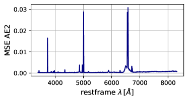
Figure 4: The pixelwise mean squared reconstruction error of the second autoencoder, i.e. the mean squared difference between its inputs and outputs. The reconstruction error is extremely small, showing that we sacrifice close to no information about the spectra by adding this second auto-encoding step.

We show examples of the input and output to the autoencoder in Figure 2 and the average pixelwise $\chi^{2}-1$ in Figure 3.

We find that the mean $\chi^{2}$ is close to unity near the middle of the spectrum and shows departures toward the edges and at the expected location of emission lines. These features are independent of the latent space dimensionality and neural network architecture we choose. This is not surprising given observational effects such as variations in throughput, detector sensitivity or sky background in particular toward the edges. Furthermore, the SDSS survey team documented 10-20% error on the error due to not accounting for the covariance between adjacent spectral bins. While the wavelength-dependent $\chi^{2}$ indicates that an optimal training would require a better description of the error covariance, particularly in spectral regions with low signal or high background, we opt to proceed with the published error model.

Upon application of the above autoencoder, we found the set of extreme outliers to be dominated by galaxies with large masked fractions (P22; their Figure 12). This effect is mitigated by inpainting a model prediction over the masked regions. For instance, Yip et al. (2004); Portillo et al. (2020) used an iterative PCA for the inpainting whereas we inpaint with the denoised spectra, $x^{\prime}$ obtained with our first autoencoder. The resulting inpainted spectra are used to train a second autoencoder of the same architecture and use the encoded distribution of this second autoencoder in the anomaly detection. We train the second autoencoder with a mean-squared error (MSE) loss as objective function,

$$\mathcal{L}_{\mathrm{AE2}}(\phi_{2},\psi_{2})=\underset{x\sim p(x)}{\mathbb{E}}\left[\frac{1}{D}\sum_{i=0}^{D-1}\left(x^{\prime}_{i}-g_{{\psi_{2}}}[f_{\phi_{2}}(x^{\prime})]_{i}\right)^{2}\right].$$ (5)

The training of the second AE is initialized with the weights from the first AE. We find in our experiments that the pixelwise mean squared error of this autoencoder is extremely low (Figure 4), demonstrating that practically no information about the spectra is lost in this additional step. We note that other deep learning approaches that motivate robustness to data corruptions, such as contrastive learning might be employed instead of two autoencoders. We choose AEs in order to evaluate the reconstruction error as an additional anomaly metric.

3.2.2 Density Estimation

We then move on to fit a normalizing flow to the encoded distribution of the second AE. A plethora of normalizing flow models have been proposed in the literature. Here, we use a Sliced Iterative Normalizing Flow (SINF) (Dai & Seljak, 2021). The concept behind this flow is to identify directions in which the difference between the current and target marginal distributions are maximal and fit transformations to reduce this difference one direction at a time. SINF achieves state-of-the-art results on standard machine learning datasets and requires little to no hyperparameter tuning.

3.2.3 Conditional Density by Spectral Class

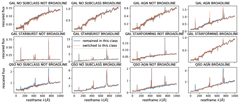
Figure 5: Examples of spectra that switch class in the relabeling process. For each class (each panel) we show a spectrum that was newly assigned to this class in red together with a similar spectrum that remained in the class (blue).

Galaxy spectra form a very diverse data set. To better organize the results of our algorithm we separate spectra by their spectral class and perform anomaly detection conditional on the class. We start by using pre-defined classes assigned by the SDSS pipeline and provided in the CLASS and SUBCLASS parameters. The class parameter separates the data set into quasars and galaxies. Galaxies can be assigned an additional subclass parameter, which is determined by their line ratios and widths. The subclass parameters are STARFORMING, STARBURST and AGN. An additional parameter BROADLINE is used to label spectra with emission lines that surpass a certain width threshold . We use these class labels (first and second row in Table 1) to train a conditional density estimator, which estimates the conditional probability of each encoded data point, $p(z|\mathrm{class})$. The bounds that determine the SDSS classes are sharp cutoffs in a continuous space. For our application, the exact definition of the classes are irrelevant, instead we are interested in grouping spectra by similarity. We therefore define new classes by reversing the process after training the density estimator on the pipeline assigned labels: We use the trained density estimator to determine the most likely class of each spectrum under the model,

$$\mathrm{class_{max}}=\underset{\mathrm{class}\in\mathrm{classes}}{\mathrm{argmax}}\left[\log p_{\varphi}(z|\mathrm{class})\right].$$ (6)

We find that a very small fraction (0.75%) of spectra were assigned a different CLASS from galaxy to QSO or vice versa but about $25\%$ of spectra are assigned to a new SUBCLASS in this process. These changes are mostly minor in the sense that the new labels tend to be similar to the original ones. We show examples of spectra that change class (CLASS$+$SUBCLASS) under this reassignment alongside their nearest neighbor among the spectra that remained in the newly assigned class in Figure 5. This demonstrates that the relabeling indeed assigns spectra to new classes by similarity.

We retrain the density estimator on the new labels. The re-labeling step is not strictly necessary, since we marginalize over all possible classes for our anomaly detection. However, having less ‘noisy’ labels during training helps the density estimator reach lower loss and thus higher accuracy. The number of objects in each class is tabulated along with an assigned galaxy category to broadly split the test sample into quiescent galaxies, star-forming or AGN host (SF/AGN) galaxies and QSOs (Table 1).

Label	Class Label Name	Category	N
0	GAL NO SUBCLASS NOT BROADLINE	quiescent	60427
1	GAL NO SUBCLASS BROADLINE	quiescent	11991
2	GAL AGN NOT BROADLINE	SF/AGN	8017
3	GAL AGN BROADLINE	SF/AGN	1217
4	GAL STARBURST NOT BROADLINE	SF/AGN	11835
5	GAL STARBURST BROADLINE	SF/AGN	107
6	GAL STARFORMING NOT BROADLINE	SF/AGN	39319
7	GAL STARFORMING BROADLINE	SF/AGN	3168
8	QSO NO SUBCLASS NOT BROADLINE	QSO	186
9	QSO NO SUBCLASS BROADLINE	QSO	1012
10	QSO AGN NOT BROADLINE	QSO	396
11	QSO AGN BROADLINE	QSO	253
12	QSO STARBURST NOT BROADLINE	QSO	74
13	QSO STARBURST BROADLINE	QSO	1212
14	QSO STARFORMING NOT BROADLINE	QSO	13
15	QSO STARFORMING BROADLINE	QSO	415

Table 1: List of labels with the label number, class label name, assigned galaxy category and the number of galaxies from the test set for each class after the relabeling step.

3.2.4 Anomaly Score

Our final anomaly score, $\mathrm{AS}_{PAE}$, is the probability of a data point marginalized over all possible classes

$$\mathrm{AS}_{PAE}=-\log p_{\varphi}(z)=-\log\sum_{\mathrm{classes}}p_{\varphi}(z|\mathrm{class})p(\mathrm{class}),$$ (7)

where the prior $p(\mathrm{class})$ is determined by the frequency of each class in the training set (after re-labeling). We use the scipy’s (Virtanen et al., 2020) logsumexp function to perform the marginalization in a numerically stable manner.

3.3 PAE architecture and training

Parameter	Value Range	Scale	Value
Network Depth	$[2,5]$	lin	2
FC Units	$[\mathrm{Latent\,Size},\mathrm{Layer\,Input\,Size}]$	lin	100,590
Latent Size	$[2,14]$	lin	10
Dropout Rate	$[1\times 10^{-3},0.5]$	log	0
Initial L-Rate	$[1\times 10^{-4},2\times 10^{-3}]$	lin	$7\times 10^{-4}$
Final L-Rate	$[5\times 10^{-6}$, Initial L-Rate]	log	$1.3\times 10^{-5}$
Decay Steps	$[2000,40000//\mathrm{Batch\,Size}\times 10]$	log	2300
Optimizer	[Adam, RMSprop, SGD]	-	Adam
Batch Size	$[16,256]$	lin	33

Table 2: Parameters governing the autoencoder network architecture and training procedure that were optimized in order to achieve low reconstruction error. The values used in the analysis are listed in the last column.

We choose a standard multilayer perceptron (MLP) architecture for the autoencoder, which we found to reach lower reconstruction error than convolutional architectures, but verified that other architectures result in anomaly scores that are highly correlated with the presented results. The architecture and training parameters are optimized with OPTUNA (Akiba et al., 2019), an automatic hyperparameter optimization software framework for machine learning. We run ca. 1500 training trials over 10 epochs to sample the network performance measured in terms of the validation loss as a function of these parameters. The parameters we vary, the explored ranges and (rounded) values for the best performing model are given in Table 2. We build the decoder as an exact mirror of the decoder. The best performing model consists of three layers. We optimized the number of units in the first two layers (of the encoder). Both of them are followed by a LeakyReLU activation function and Dropout layer. The last layer is a fully connected (FC) layer without activation that maps the output of the previous layers to the desired latent space dimensionality. Tests with convolutional architectures did not result in better reconstruction performance. We use a polynomial decay schedule from an initial learning rate (initial L-Rate) to a final learning rate (final L-rate) over an optimized number of decay steps. The second autoencoder stage shares the same architecture as the first one and we use the pre-trained weights from the first stage as initial values. We monitored the loss on the test set during training of the autoencoders and did not observe any overfitting. The density estimation is trained for 50 epochs. We chose the Sliced Iterative Normalizing Flow as a density estimator not only because of its proven performance, but also because it requires practically no hyperparameter tuning. The model simply adds transformation layers until the loss on the test set stops improving.

4 Results

The test set is diverse as it includes QSOs, quiescent galaxies, and SF/AGN galaxies (Table 1). After briefly investigating the distribution of properties and probability scores for each category of galaxies (§4.1), we will focus our analysis on quiescent galaxies because they represent a more homogeneous population as a starting point. By focusing on spectra that do not fall into one of the more easily defined categories with strong spectral signatures $-$ such as starburst, AGN, QSO, etc. $-$ we have a chance of uncovering some of the more subtle anomalies that the algorithm picks up and that might be difficult to identify otherwise.

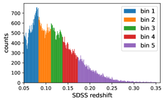
Figure 6: Redshift distribution of quiescent galaxies from the test sample and definition of redshift bins.

To stratify our analysis, we further split the test quiescent galaxy sample into five redshift bins (Figure 6) with each bin containing about 20% of the sample. This ensures that presented anomalies are not biased by redshift dependencies.

We then use both, the density-based anomaly detection score proposed in this work, $\mathrm{AS}_{PAE}$, as well as the AE reconstruction error to identify the top-eight most outlying spectra in each redshift bin (Tables 3 and  4). The anomaly detection score is good at identifying rare objects with counterparts in the training sample, whereas reconstruction error is good at detecting objects not at all represented in the training sample. We determine the most likely reason for the anomaly of each spectrum by visual inspection of the spectrum, the corresponding image, and in some cases a derivative-based sensitivity analysis. In the sensitivity analysis we take the derivative of the anomaly score with respect to the (encoded) input spectrum, and use a gradient descent method to track how the spectrum changes as we follow the gradient to higher probabilities. We discuss the most common types of anomalies in the following subsections. In some cases, a data or astronomical anomaly also results in a faulty SDSS redshift determination, exacerbating its outlier score.

Objects are referred to by their SDSS (MJD, plate, fiber).

4.1 Galaxy population global properties and probability scores

To illustrate global properties of the galaxy populations from the test set, we show in Figure 7 their bivariate distribution in terms of H$\alpha$ equivalent widths $-$ a proxy for their specific star formation rate $-$ and $\sigma_{\textrm{stars}}$ $-$ a proxy for their mass. This figure recovers a well known galaxy bimodality between star-forming and quiescent galaxies (e.g., Strateva et al., 2001; Mateus et al., 2006). On the one hand, SF/AGN galaxies tend to have high values of EW(H$\alpha$) due to ongoing star formation and/or nuclear activity. They also preferentially exhibit low and mid range values of $\sigma_{\textrm{stars}}$. On the other hand, quiescent galaxies preferentially have low values of EW(H$\alpha$) consistently with little to no ongoing star formation, and are found to reach high values of $\sigma_{\textrm{stars}}$, consistently with the majority of massive galaxies at low redshift being “quenched”.

While we expect that low-mass (and therefore low $\sigma_{\textrm{stars}}$) quiescent galaxies exist, they are much more challenging to detect owing to their faint apparent magnitudes. Therefore, the lack of their representation is likely due to survey detection limits and the difficulty in measuring extremely faint emission lines. Similarly, the lower envelope around $EW(\textrm{H}\alpha)\sim 0.5~{}$Å is due to the emission line detection limit as we impose a signal-to-noise cut of $S/N>2$ in the H$\alpha$ emission line for Figure 7. Of the 72,418 quiescent galaxies in the test sample 33,690 (47%) pass the H$\alpha$ S/N cut while the remaining 53% are not detected in H$\alpha$ or missing $\sigma_{\textrm{stars}}$ information (0.2%) and thus not shown on the figure. In contrast, the bulk of the 67,224 SF/AGN galaxies have an H$\alpha$ detection with only 0.35% failing the S/N cut. However, we note that 6,486 (9.6%) SF/AGN galaxies are not shown on Figure 7 due to unresolved (<30 km/s) $\sigma_{\textrm{stars}}$ or due to missing a DR12 value added catalog counterpart (5.6% and 4%, respectively). Despite these limitations, it is clear that the SF/AGN and quiescent galaxy populations strongly differ from one another. In fact, the difference in H$\alpha$ EW values would be even more pronounced if we could detect yet fainter emission lines.

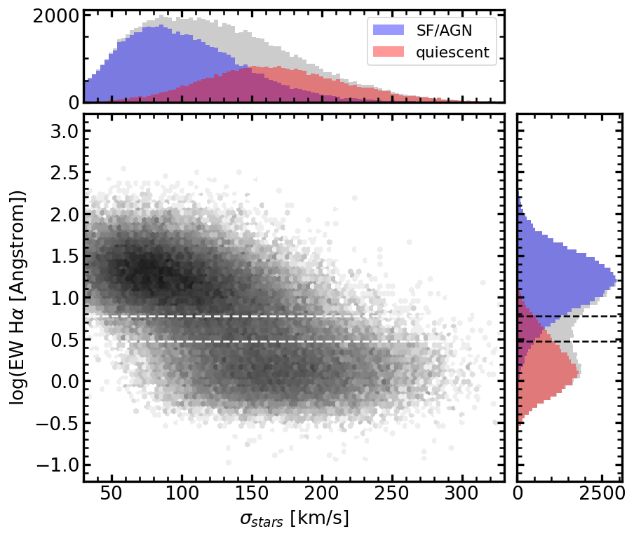
Figure 7: H$\alpha$ equivalent width as a function of the stellar velocity dispersion for the test sample. The top and side panels show the total distribution along each axis (grey) as well as the separate distributions for the quiescent galaxies (red) and SF/AGN galaxies (blue). Horizontal dashed lines correspond to 3 $\AA$ and 6 $\AA$, where there is significant overlap between the SF/AGN and quiescent galaxy populations.

The QSO category is omitted from Figure 7 because $\sigma_{\textrm{stars}}$ is not available for spectra dominated by the power-law continuum from the accretion disk as is often the case for luminous QSOs. This important difference in spectral shape also means that we expect QSO spectra to score lower values of $\log{p}$ relative to the bulk of non-QSO galaxies. To a lesser extent, we expect the SF/AGN galaxies to have a more significant tail of less probable (more anomalous) spectra due to phenomena like starbursts and strong AGN episodes that produce obvious spectral signatures such as enhanced emission line strengths and widths. Indeed, we can observe these trends by comparing the normalized distributions of $\log{p}$ values for the QSOs, SF/AGN galaxies, and quiescent galaxies (Figure 8). As expected, the quiescent galaxies (in red) have the narrowest peak with the least prominent tail toward low probability scores (i.e., high anomaly scores). This motivates our choice to focus on the quiescent galaxies in the remainder of this paper.

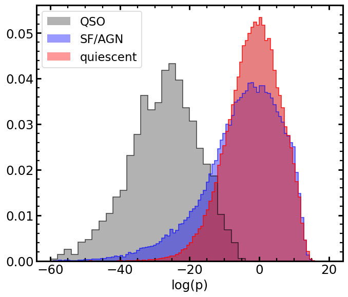
Figure 8: Distribution of $\log{p}$ values for QSOs (grey), quiescent galaxies (red) and SF/AGN galaxies (blue) in the test sample.

4.2 Identified anomalies

The anomaly score is used to identify those spectra which, after compression into latent-parameter space, have parameter values that are the least probable. The eight most anomalous spectra for the five redshift bins are listed in Table 3 and the SDSS spectrum plot (York et al., 2000; Szalay et al., 2002) of highest outlier per redshift bin is shown in Figure 9. Each panel was generated using the SDSS SkyServer and includes information on the corresponding target.

The original spectrum, its reconstruction, and the closest training spectrum along the path in latent parameter space that maximizes $\log{p}$ ascent were visually inspected for each of the forty outliers. The anomalies can be categorized as follows. In some cases the reconstructions are poor, indeed six objects that are extreme anomalies also appear in the extreme reconstruction outlier list to be introduced in §4.3; it is not surprising that their latent parameters are improbable. In other cases, the reconstruction is good, the slope of ascent in $\log{p}$ with respect to the latent parameters is large, and it is clear by the difference between the spectra along the ascent which features are “anomalous”. In most cases, the reconstruction is good but the slope of $\log{p}$ is shallow, and produces only subtle differences between the spectra. These objects lie at the tail of a continuous distribution.

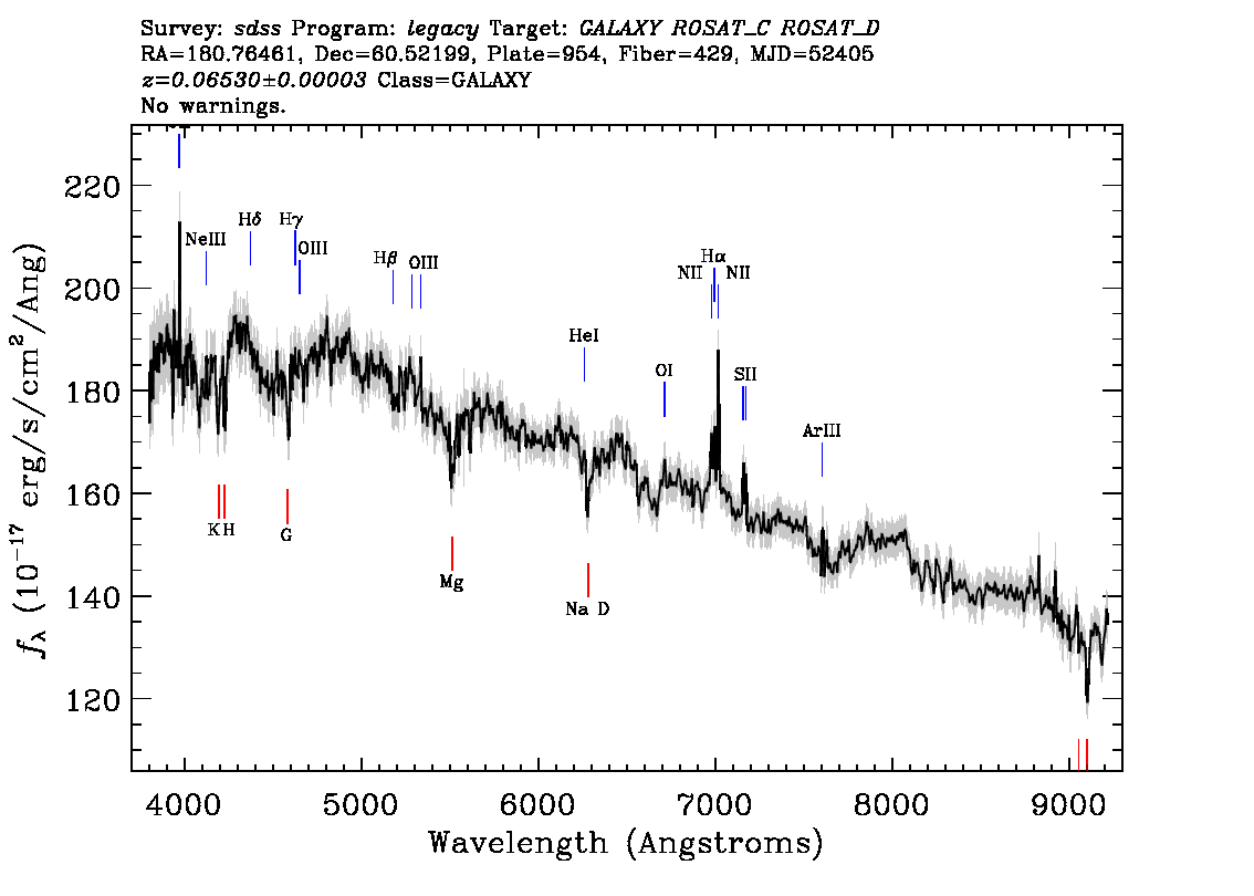
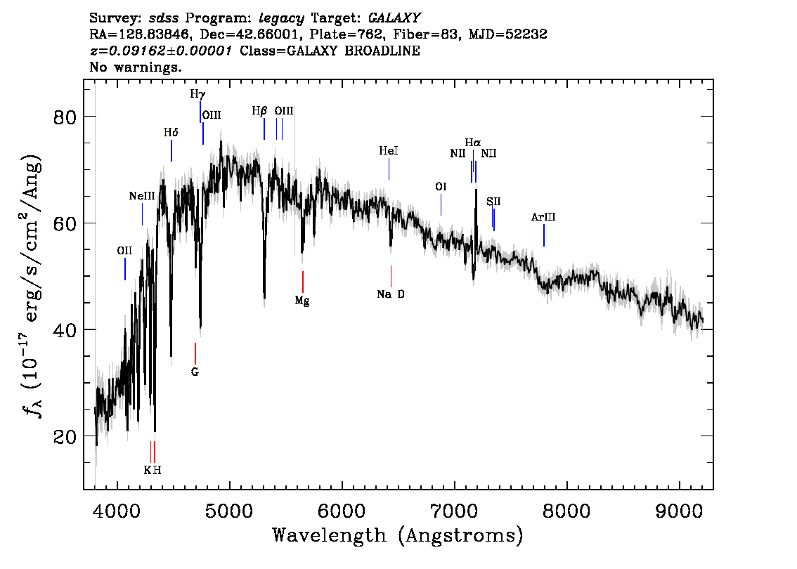
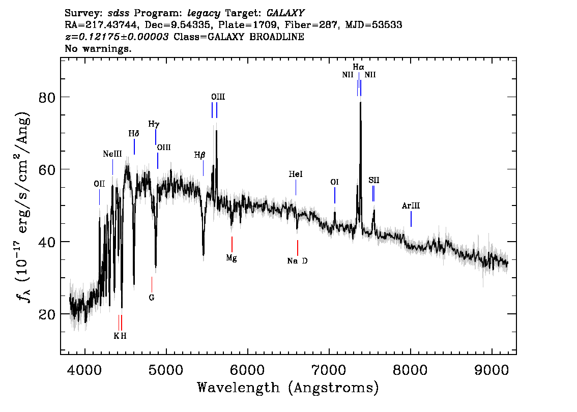
Figure 9: The most anomolous spectrum for each of the five redshift bins, with increasing redshift going from top left to bottom right. Each panel, generated with the SDSS SkyServer, shows the original spectrum in gray, a smoothed version in black, and labels at the expected location of emission and absorption lines in blue and red, respectively. Information on each target is listed above its corresponding spectrum.

In the following subsections, we identify the physical causes that make the outliers outliers. In a few cases, physical effects give rise to an incorrect redshift, which in turn exacerbates the outlier appearance of these sources.

4.2.1 AGN/QSO

There are two objects that are visually clear outliers that can be assigned as AGN. Object (52405, 954, 429) is the top outlier in redshift bin 1 and is shown in Figure 9. Its spectrum is dominated by a strong blue continuum with comparatively weak emission lines relative to typical QSOs. This object was targeted by SDSS as a ROSAT source (Boller et al., 2016) that is bright and/or moderately blue (ROSAT_C) and also bright enough for follow-up spectroscopy (ROSAT_D). It has been classified as a BL Lacertae object (Anderson et al., 2007; Plotkin et al., 2008), which is a rare QSO sub-type. This classification is reported in the SIMBAD astronomical database (Wenger et al., 2000), and differs from both the SDSS pipeline and PAE classification as a GALAXY. The erroneous spectral types and large anomaly score likely all arise from the unusual spectral shape which appears somewhat intermediate between a featureless BL Lac blazar (BZB) spectrum and a BL Lac Galaxy-dominated (BZG) spectrum as defined by de Menezes et al. (2019) and lacks strong broad QSO lines.

The SDSS redshift of the second clear AGN/QSO outlier is incorrect. Object (53084, 388, 1440), whose spectrum is shown in Figure 10, is identified as a broadline galaxy at $z=0.05$ by SDSS though it was targeted as and is in fact a quasar at $z=1.84$. The PAE reconstruction of this object is also poor. This is expected as such a catastrophic redshift failure would not be represented in the training dataset, and our approach does not vary the redshift and assumes correct rest-frame wavelengths.

Figure 10: Left: Spectrum of object (53084, 388, 1440), an anomaly identified by our pipeline, which is a quasar assigned to an incorrect redshift and incorrect spectral type by the SDSS pipeline. Right: Spectrum of object (54141, 2513, 264), the one example that is unlike the others in the E+A anomaly sample, due to its extremely blue color and its lack of prominent [NII] lines. This object was targeted by SDSS as a GALAXY; it was also tagged as being in an area of QSO color-color space with a high contamination rate, hence the QSO_REJECT label.

More AGNs and quasars among our outliers that share distinguishing features are described in subsequent subsections.

4.2.2 E+A Galaxies

The majority of the outliers are visually classified as E+A galaxies, whose spectra exhibit both old (elliptical) and young (represented by A stars) stellar populations (Dressler & Gunn, 1983). They are characterized by having deep Balmer absorption lines but no significant [O II] emission, indicative of being post-starburst (see review by French, 2021, and references therein). Objects (53533, 1709, 287) and (53534, 2112, 512) shown in Figure 9 are examples of this type of outlier.

Almost all of these objects exhibit the presence of [N ii] and weak to absent H$\alpha$, and so are classified as either AGN or galaxy with a low-ionization nuclear emission-line region (LINER; Heckman, 1980) based on their spectral features and/or position on the BPT emission-line diagnostic diagram (Baldwin et al., 1981). Three of the E+A galaxies, including (53533, 1709, 287), also have a prominent [OIII] line, putting them into the AGN class. Note that Meusinger et al. (2017) find that only 2-3% of E+A galaxies are found to host AGNs using conventional search criteria.

From among this class of outliers, one stands out as being particularly unlike the others. Object (54141, 2513, 264) is extremely blue, dominated by the spectra of OBA-type stars, and does not have [N ii] emission. The spectrum of this object is shown in Figure 10. The optical image from the Legacy Surveys (LS; Dey et al., 2019) Sky Viewer shows the galaxy to be blue, diffuse, and asymmetric, indicating possible tidal interaction.

We conclude that E+A galaxies with evidence of AGN activity through their significant [N ii] emission are relatively rare in our sample and these spectra that make the top outlier list represent the extreme tail of their distribution. Indeed, these are the rare galaxies that bridge the dominant populations of red inactive galaxies and blue galaxies with significant star formation (Meusinger et al., 2017).

4.2.3 [N ii] emission/LINERs

Most of the anomaly sample have a high [N ii]/H$\alpha$ ratio, with almost all of those exhibiting weak to no [O iii], H$\alpha$, nor H$\beta$ emission. Based on these features, these anomalies are identified as LINERs, as distinguished from star-forming galaxies and normal AGNs, based on their inferred position in the BPT diagram (Baldwin et al., 1981).

In details, different mechanisms have been proposed to explain LINER-like spectral signatures such as weak AGNs (Ho, 2008) or retired galaxies with spectra dominated by an aging stellar populations with gas ionized by low-mass stars (Cid Fernandes et al., 2011). Similarly, Agostino et al. (2021) recently presented an approach to distinguish two sub-populations differing in the hardness of the ionization field (dubbed soft and hard LINERs). While a detailed investigation is beyond the scope of this exploratory work, the identification of LINER-like spectra as PAE anomalies could motivate future effort.

4.2.4 Neighboring Contaminating Sources

Inspection of LS DR9 optical imaging using the LS Sky Viewer showed four cases of a secondary source within the fiber aperture placed at the primary target. An example is (53054, 1436, 407), shown in Figure 9, which looks like an M star overlapping a galaxy. This object is also selected as having a poor reconstruction, as seen in Figure 13: the features of the M star are not accommodated by the PAE model. The odd occurrence of multiple sources entering a fiber has already been documented in Bolton et al. (2012), who present example contaminated spectra from the BOSS Survey.

In addition, there were a number of cases of possibly overlapping sources. Spectroscopically, the visual characteristic for these anomalies is a slight tilt in the observed continuum color relative to the reconstructed continuum color.

4.2.5 Supernovae

One outlier is SN2001km, a Type Ia supernova discovered by Madgwick et al. (2003).

There are other supernovae in our sample previously identified using template-based (not machine learning) algorithms (Madgwick et al., 2003; Graur & Maoz, 2013). The distribution of their anomaly scores is poor relative to the general population, but are not isolated in the tail. The PAE outlier criterion in this work was not tailored to identify known SNe within SDSS spectra, but the procedure could be adapted and calibrated to be more sensitive to a specific type of anomaly such as supernova. Curent machine-learning methods tailored for supernova detection and classification in spectra (e.g. Muthukrishna et al., 2019; Palmese et al., 2021) are based on supervised learning.

4.2.6 Local low surface brightness galaxies

Object (53520, 1657, 126) is one of four sources with similar and poor PAE reconstructions, which we show in §4.3.6 to be local ($z<0.1$) low surface brightness galaxies. Of these four, only this one had a top-8 anomaly score. Note that some other sources with poor PAE reconstructions that have been identified as QSO, supernova, or overlapping sources, also have top-8 anomaly scores. Generally, however, objects with extreme reconstruction errors do not necessarily find themselves in the top anomaly list.

4.2.7 Externally classified Active Galaxies

In this subsection we depart from discussing anomalous features identified within the SDSS spectra, but rather refer to AGN classifications reported by SIMBAD based on X-ray data.

Seventeen outliers are identified in SIMBAD as LINER, AGN or QSO. Of these, slightly more than half are “E+A” galaxies. The remaining “AGN” outliers are weak-line radio galaxies (Hine & Longair, 1979; Tadhunter et al., 1998; Buttiglione et al., 2010), classified as radio-loud AGN whose optical spectra the appearance of an old elliptical galaxy and no or weak [O iii] emission. An example of such a spectrum is shown in Figure 11. All of the weak-line radio galaxies exhibit [N ii] emission and no H$\alpha$, to which we attribute to a LINER rather than an AGN classification.

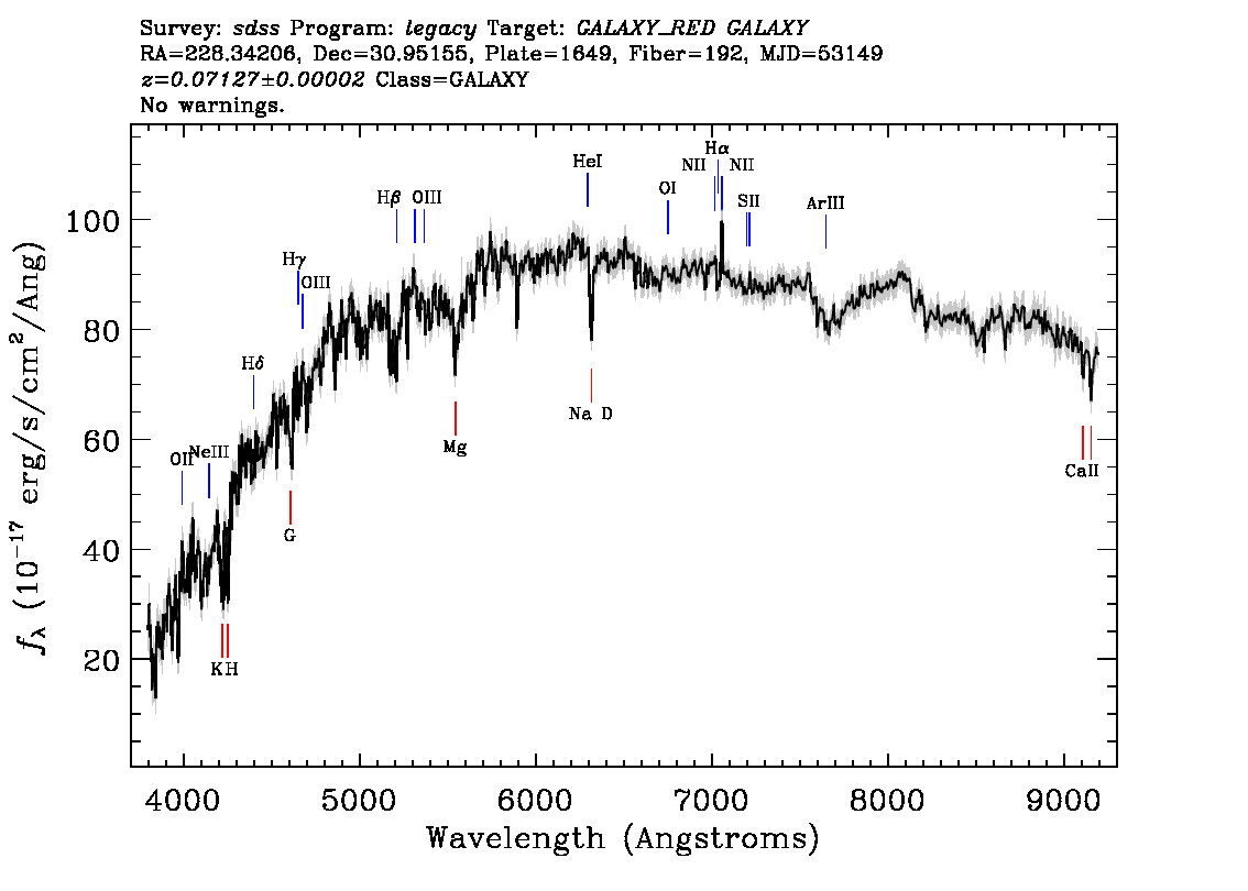
Figure 11: Spectrum of object (53149,1649,192) from the SDSS SkyServer. The source is labeled as a LINER in the SIMBAD database and the spectrum is that of an elliptical galaxy. Note the presence of [N ii] emission and the absence of H$\alpha$.

4.2.8 Comparison with Previous Work

Baron & Poznanski (2017) [B17] performed outlier detection on SDSS data. They trained a random forest labeling real data and synthetic spectra drawn from the per-feature distribution of the real data and no covariance between features. Outliers were then identified in a metric space based on distance between their nodes in the forest.

The samples in which we and [B17] search for outliers are significantly different. We restrict our redshift range, use a higher data resolution, and divide the spectra into training and test samples. In this article we focus on the subset of galaxies that are not classified as STARFORMING, STARBURST, or AGN, whereas [B17]’s approach is particularly sensitive to sharp emission lines that would often put a galaxy in one of the above classes.

Considering these differences, the classes of outlier identified in both works are identical. One class are E+A Galaxies with strong Balmer absorption, both with and without ongoing star formation. [B17] find a class of outliers in the BPT diagram, at the edges of both [OIII]/H$\beta$ and [NII]/H$\alpha$. Our outliers rarely exhibit either [OIII] or H$\beta$ emission (a large fraction having Balmer absorption) but we have identified high [NII]/H$\alpha$, which we associate with AGN. Strong NaID absorption appears in many of the outliers we associate with AGNs. Other common outlier classes are SNe, blends, calibration errors. Our extremely red outliers have been associated with a red background source seen in imaging.

Portillo et al. (2020) used VAE as a method to reduce the dimensionality of SDSS spectra. The focus was on the quality of their reconstruction and identifying tracks in their latent space that traverse astrophysical classes of objects. Their top ten outliers are explained as stars that were erroneously classified as galaxies, low SNR, contaminating neighbor, missing data, and poor calibration.

Pat et al. (2022, hereafter P22) used the same training and test sets as this work and employed a similar method except that they included only one round of AE therefore skipping the in-painting step. That earlier work also did not employ labels for conditional probability estimation, and was thus more subject to probability density scores being affected by the relative importance of QSO and galaxy populations. As a result, the most outlier spectra tended to be biased toward cases with a higher fraction of masked pixels and/or QSO spectra (see their Figure 12). While that work was not focused on identifying outliers, noting these behaviors has helped improve our choices for the present experiment aiming at finding outlier spectra among subsets of galaxies (specifically quiescent galaxies in this work).

More recently, Liang et al. (2023, hereafter L23) presented an overall similar study to that of P22 and to this work. Despite the general similarity, two notable differences lead to slightly distinct and complementary results. These authors used the SPENDER neural network architecture (Melchior et al., 2022) to train a model of SDSS spectra and inspect outliers. The first important difference is that L23 added a loss term to account for redshift variations whereas we opted to split the sample into redshift bins. The second difference is that we employed a conditional density estimation based on labels whereas L23 did not use labels $-$ more similarly to P22. To compare the results we combined the catalog from L23 with our test set, finding 132,257 common entries among our test set of 139,642 (95%). In particular, we focus on the subset of 71,703 quiescent galaxies and show a comparison of the $\log{p}$ values from L23 and from this work in Figure 12. Each panel corresponds to a redshift bin increasing from left to right as labeled.

The outliers based on their anomaly scores from this work are shown with blue circles and they tend to also be outliers according to the L23 model. This implies that the two trained models are largely consistent in their outlier detection. We also note differences that we attribute to the distinct decisions described earlier. Namely, the difference in using a loss term to correct for redshift (L23) versus splitting the sample into redshift bins (this work) manifests itself as a redshift dependent offset when comparing directly $\log{p}$ values (one-on-one dotted line). The second difference is that the use (or absence) of conditional probability results in the QSO (small orange dots) being more heavily biased toward a tail of outliers in the L23 model compared to this model. There are advantages and disadvantages to each set of decisions, which ultimately needs to be tailored to the science question at hand.

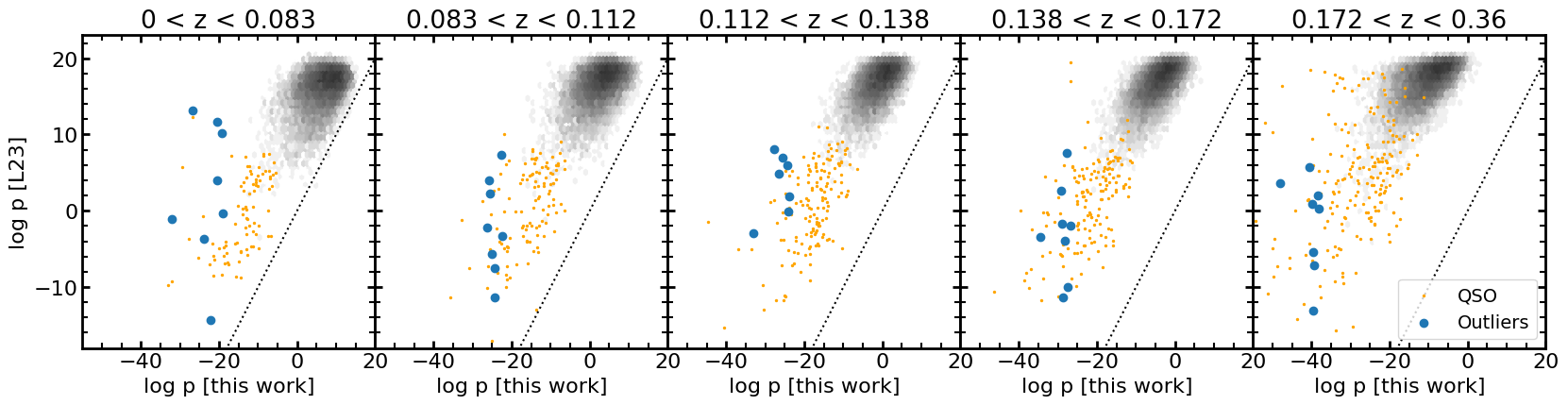
Figure 12: Comparison of the $\log{p}$ values from L23 and from this work for the overlapping sample of 71,703 quiescent galaxies (grey shaded bivariate distribution) split into the five redshift bins used in this work. The redshift ranges increase from left to right as labeled. We show the outliers based on the lowest anomaly scores from this work (blue filled circles) and the 771 overlapping QSO spectra (orange dots). The black dotted line corresponds to the one-to-one relationship.

4.3 Most outlying reconstruction error

We define reconstruction error as the masked and inverse-noise weighted L2-distance between the original input spectrum and the output of the second decoder

$$RE_{PAE}=\sum_{i=0}^{D-1}M_{i}\frac{\left(x_{i}-g_{\psi_{2}}[f_{\phi_{2}}(x^{\prime})]_{i}\right)^{2}}{\sigma_{i}^{2}}.$$ (8)

The eight spectra with highest reconstruction error for the five redshift bins were identified and visually inspected. These spectra are given in Table 4. In this subsection, we discuss sources of reconstruction error in these forty spectra that were identified by humans. We do not plot the largest outlier for each redshift bin as was done for anomaly detection, as they do not fairly represent cases of interest.

4.3.1 Airglow

Four outliers occur on Plate/MJD 362/51999 that exhibit [OI] airglow emission lines at observer-frame 6302, 6365Å. Of these, three are the largest outlier in their respective redshift bin. Inspection of other spectra not in our top 40 list but taken in this exposure exhibit the same lines.

4.3.2 Contaminating Sources

Images of eighteen of the forty outliers exhibit the clear overlap of distinct astronomical sources. While the spectral features of the dominant source upon which the fiber is centered is well reconstructed by the PAE, the continuum is not.

One example already noted in §4.2.4 is object (53054, 1436, 407), an M star overlapping a galaxy. Its poor reconstruction, shown in Figure 13, demonstrates that the PAE model does not simultaneously accommodate the combination of M star and galaxy.

Two other outliers exhibit problems with the reconstruction of their continua, though visual inspection could not confirm nor preclude the presence of a neighboring contaminant.

4.3.3 QSO with Foreground absorption – Bad $z$

Two objects are quasars misclassified by SDSS as galaxies at incorrect redshifts. Object (53084,1440,388) is a quasar at $z=1.838$ but has an SDSS redshift of $z=0.05146$. (53167,1423,287) is at $z=1.965$ but has an SDSS redshift of $z=0.08944$. Absorption lines assigned to Hydrogen as the nominal SDSS redshifts are responsible for these misclassifications.

One of our first processing steps is to blueshift the spectra, so it is expected that catastrophic redshift errors produce outlier spectra.

4.3.4 Red continuum

One red galaxy, Object (52262, 743, 561) shown in Figure 13, has a continuum that is bluer than its PAE reconstruction. The SDSS colors of this galaxy are extremely red: $u-g=2.8$ mag, $g-r=1.51$ mag, $g-i=2.39$ mag, which is an extreme red outlier . As evidenced in the reconstructed spectrum, the PAE can accommodate spectra redder than the data.

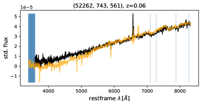
Figure 13: Two objects with visually clear reconstruction error. The black curve is the data and the orange is the reconstruction. Left: Object (52262, 743, 561) has extreme red colors relative to the entire SDSS sample. Right: Object (53054, 1436, 407) appears to include an overlap of an M star and an emission line galaxy in the same fiber. The reconstruction does not reproduce any of the M star features. Masked pixels are indicated by blue vertical lines.

4.3.5 Supernova

SN2001km, already identified as highly anomalous in §4.2.5, also has large reconstruction error. In addition, Object (53770, 2376, 183) is SN 2006af discovered by the spectroscopic search of Graur & Maoz (2013).

4.3.6 Low-redshift, low surface brightness galaxies

Four spectra have reconstructions that look nearly identical to each other but do not look like the data. The spectrum and reconstruction are similar in that they both have high-frequency ‘noise’ fluctuations but are otherwise dissimilar in both their broad and narrow band features. The reconstruction error is catastrophic, as seen by the high scores in Table B1.

The imaging and spectra of these four objects share common features, as shown in Figure 14. Their spectra are characterized by narrow, unresolved emission lines and their continua show a red slope with noticeable noise likely due to the low surface brightness of the galaxy. They all share the same SDSS-determine redshift of $z=0.05$. The reconstructed spectra of all four objects are similar to each other but are dissimilar to the original data. The images show that the galaxies are characterised by a low surface brightness with a red central region upon which the SDSS fiber is placed. Those features are unusual relative to the majority of normal low-redshift galaxies with H$\alpha$ emission lines, which instead tend to be galaxies with star formation, blue continuum slopes and a higher surface brightness.

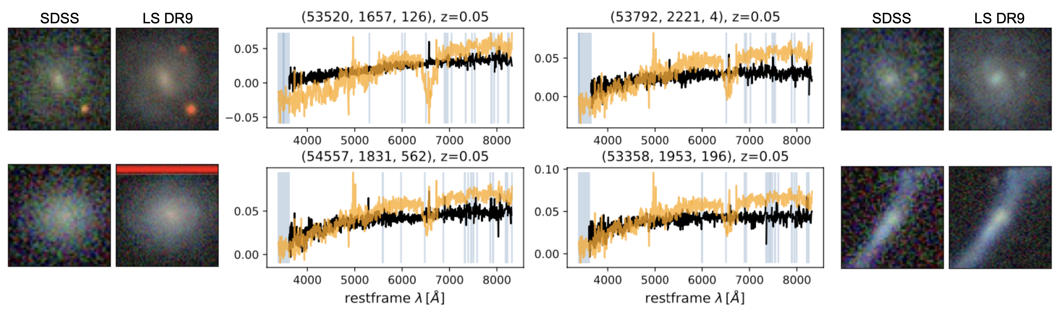
Figure 14: Imaging and spectra of four select objects, (53520, 1656, 216), (53792, 2221, 4), (54557, 1831, 562), and (53358, 1953, 196), that have large reconstruction errors and similar observed properties. In the spectra, the black curve is the data, the orange is the reconstruction and the blue vertical lines indicate the masked pixels. The images are 20″$\times$ 20″cutouts from SDSS Imaging and the Legacy Survey DR9. (the SDSS fiber diameter was 2″)

Recall from §4.2.4 that we found that autoencoding the output of a previous autoencoding (Eqs. 4, 5), effectively interpolates the masked regions in the input spectra. Large reconstruction errors in cases such as Object (53520, 1657, 126) do not occur in the output of the first autoencoder.

4.3.7 Misextraction

Both (53473, 1627, 374) and (54154, 2497, 491) have sharp negative flux lines and (52443, 986, 297) has a deep absorption adjacent to a sharp emission line that has been masked. The spectrum of Object (51614, 281, 34) has asymptotically increasing red flux. This source was observed in the DESI survey (DESI Collaboration et al., 2016b); the spectra look similar except that DESI does not exhibit a red runaway.

5 Conclusions

We have demonstrated that a Probabilistic Autoencoder is able to learn the complex intrinsic distribution of galaxy spectra and can be used to identify rare and outlier objects from a set of SDSS spectra. When examining the histogram of probabilities, we find that the model on average assigns lowest probabilities to quasars, which is expected, given their respective rareness in our training sample and large intrinsic variability. The mean probabilities of SF/AGN galaxies and quiescent galaxies are similar, but SF/AGN galaxies exhibit a longer tail to small probabilities and quiescent galaxies have the narrowest peak.

Focusing on galaxies previously labeled as generic galaxies by the default SDSS classifier, we find that the majority of the rare objects have significant Balmer absorption, no [OII] emission, but exhibit [NII] emission. These are associated with the rare E+A galaxies with evidence of AGN activity described by Meusinger et al. (2017).

The PAE also identifies expected anomalies, such as blends of multiple sources and supernovae. In addition to these expected anomalies, the PAE picked out two singular objects, one an extremely blue E+A galaxy and the other a spectral mix of an early elliptical and emission-line galaxy.

The PAE implementation used in this work includes a conditional density estimation, which can be used to incorporate data labels and additional information such as spectral classes. In reverse, this conditional model allows us to perform a probabilistic classification of unlabeled objects. Generally, because of its probabilistic layout, the PAE can be used as part of a larger probabilistic framework, such as a Bayesian parameter inference pipeline (demonstrated in  Stein et al. (2022)).

In the current form the PAE anomaly detection is not tailored toward a specific type of outlier, for example, neither the low-probability nor outlier-reconstruction scores accentuate the peculiarities of supernovae relative to other outliers. The method could be tailored to a specific anomaly, e.g., through calibration or suitable probabilistic conditioning.

In principle, the ranking of rarity of the anomaly detector is sensitive to the training data, its preprocessing, and the dimensionality of the encoded space. However, we find that the rankings for different model architectures and different random seeds are highly correlated.

When using reconstruction errors as an outlier detection metric, we find that the results are sensitive to large point deviations away from the learned spectral behavior. These can be caused by misextractions and unanticipated issues with the observation itself. Conversely, large errors are also caused by subtle differences that persist over large ranges of wavelength, which can be cased by a faint background source contaminating the primary source signal. In addition, we find that reconstruction can sometimes fail for the noisier data in our sample.

Data Availability

The data underlying this article were accessed from the SDSS-BOSS DR16 release (York et al., 2000; Strauss et al., 2002; Richards et al., 2002; Gunn et al., 2006; Ahumada et al., 2020) available at https://skyserver.sdss.org/dr16/en/home.aspx. The derived data generated in this research will be shared on reasonable request to the corresponding author.

Appendix A Top Anomalies

Table 3 presents the eight objects for each redshift bin with the highest anomaly score. The peculiar features described in §4.2 associated with each outlier are given in the ‘explanation’ column. AGN/QSO are visually identified as an AGN or quasar. E+A galaxies are characterized by Balmer absorption. LINERS are galaxies with a high [NII]/H$\alpha$ ratio, and generally have no other strong emission lines. ‘Neighbor‘ indicates the presence of multiple sources entering the fiber. ‘SN’ refers to a previously identified supernova. Low SB refers to one galaxy with a noticeably low surface brightness and red center. Objects with SIMBAD LINER, AGN, or QSO classification are labeled with brackets, e.g. ‘[AGN]’.

MJD	fiber	plate	z	z-bin	logp	explanation
52405	429	954	0.07	1	-32.11	AGN.QSO, [AGN]
51691	640	350	0.08	1	-26.84	LINER
51820	45	429	0.07	1	-23.78	LINER, [AGN]
51955	247	472	0.07	1	-22.17	SN
52258	399	412	0.07	1	-20.49	E+A, LINER, [QSO]
53520	126	1657	0.05	1	-19.38	Low SB
53149	192	1649	0.07	1	-19.16	LINER, [LINER]
53084	388	1440	0.05	1	-19.14	AGN/QSO, [QSO]
52232	83	762	0.09	2	-25.72	E+A, LINER
53386	368	1755	0.11	2	-25.54	E+A, LINER
54141	264	2513	0.11	2	-25.18	E+A, LINER
51882	11	435	0.1	2	-24.36	E+A, LINER, [AGN]
54561	586	1833	0.1	2	-24.34	E+A, LINER, [AGN]
53729	142	2236	0.09	2	-22.62	Neighbor
51984	374	498	0.09	2	-22.52	E+A, LINER, [AGN]
52991	533	1270	0.08	2	-20.4	E+A, LINER
53533	287	1709	0.12	3	-33.14	E+A, LINER, [AGN]
51986	81	294	0.12	3	-27.78	E+A, LINER
53327	603	1928	0.13	3	-26.46	E+A, LINER
52964	91	1587	0.11	3	-26.19	E+A, LINER, [LINER]
53469	205	2099	0.13	3	-25.69	E+A
51873	487	443	0.13	3	-24.35	E+A
52000	259	288	0.12	3	-24.18	Neighbor
51930	256	285	0.12	3	-23.84	E+A, LINER
53054	407	1436	0.14	4	-34.58	Neighbor
53386	163	1755	0.14	4	-29.26	E+A, LINER
51930	115	285	0.17	4	-28.88	LINER, [AGN]
52615	233	961	0.16	4	-28.77	E+A, LINER, [LINER]
51929	115	470	0.16	4	-28.14	E+A, LINER
53089	114	1623	0.17	4	-27.84	E+A, LINER
52672	4	934	0.14	4	-27.53	LINER, [AGN]
54589	77	2532	0.14	4	-26.9	Neighbor
53534	512	2112	0.29	5	-48.2	E+A, LINER
52238	530	757	0.29	5	-40.6	LINER
52368	575	607	0.24	5	-39.93	E+A, LINER, [LINER]
52724	234	1195	0.23	5	-39.56	E+A, LINER
53875	327	1805	0.25	5	-39.51	LINER [AGN]
52056	446	610	0.24	5	-39.26	Neighbor
53358	184	1953	0.26	5	-38.29	E+A, LINER, [LINER]
53358	199	1750	0.21	5	-38.23	E+A, LINER, [LINER]

Table 3: Spectra contained in the test set that were identified as anomalous because of their low probability.

Appendix B Top Reconstruction error

Table 4 presents the eight objects for each redshift bin with the highest reconstruction error. The peculiar features described in §4.3 associated with each outlier are given in the ‘explanation’ column. Several objects in the same exposure exhibit lines associated with ‘Airglow’. Four ‘Low SB’ objects exhibit low surface brightness star forming regions and a red galaxy center leading to spectra with an unusual combination of a noisy red continuum with narrow emission lines with poor reconstructions that do not look like the original spectra. ‘QSO-Foreground’ have an incorrect SDSS redshift due to foreground absorption lines.

MJD	fiber	plate	z	z-bin	recon error	explanation
51999	37	362	0.06	1	96.16	Airglow
53520	126	1657	0.05	1	25.57	Low SB
53792	4	2221	0.05	1	15.63	Low SB
53084	388	1440	0.05	1	14.39	QSO-Foreground
51955	247	472	0.07	1	9.93	SN
54557	562	1831	0.05	1	8.94	Low SB
53358	196	1953	0.05	1	8.3	Low SB
52262	561	743	0.06	1	7.21	Red
51999	72	362	0.1	2	20.8	Airglow
53167	287	1423	0.09	2	5.46	QSO-Foreground
53473	374	1627	0.09	2	4.35	Misextraction
53729	142	2236	0.09	2	3.56	Subtle (Neighbor)
53327	499	1928	0.08	2	3.54	Subtle (Neighbor)
53770	183	2376	0.09	2	3.3	SN
52443	297	986	0.09	2	3.17	Misextraction
52441	60	790	0.1	2	2.93	Subtle (Neighbor)
52000	259	288	0.12	3	4.44	Subtle (Neighbor)
53494	379	1829	0.12	3	3.28	Subtle (Neighbor)
51614	34	281	0.13	3	3.24	Misextraction
54464	360	1876	0.13	3	2.97	Subtle (Neighbor)
51999	273	362	0.12	3	2.8	Airglow
51908	301	450	0.12	3	2.62	Subtle (Neighbor)
53379	43	1752	0.12	3	2.46	Subtle (Neighbor)
54154	491	2497	0.12	3	2.33	Misextraction
51999	20	362	0.14	4	8.72	Airglow
53054	407	1436	0.14	4	5.06	Neighbor
51959	428	541	0.16	4	4.88	Subtle (Neighbor)
51820	210	429	0.16	4	2.82	Subtle (Neighbor)
53149	595	1570	0.15	4	2.49	Subtle
54178	43	2492	0.14	4	2.43	Subtle (Neighbor)
51993	166	334	0.16	4	2.41	Subtle
52465	473	1043	0.14	4	2.22	Subtle (Neighbor)
52345	483	613	0.18	5	3.34	Subtle (Neighbor)
53504	119	1828	0.19	5	3.22	Misextraction
54510	524	2150	0.18	5	3.21	Subtle (Neighbor)
51671	460	348	0.21	5	3.07	Subtle (Neighbor)
53818	291	2013	0.21	5	2.81	Subtle (Neighbor)
53815	177	2427	0.22	5	2.65	Misextraction
53682	16	2268	0.19	5	2.48	Subtle (Neighbor)
53035	421	1735	0.21	5	2.44	Subtle (Neighbor)

Table 4: Spectra contained in the test set that were identified as anomalous because of their high reconstruction error

References

- Agostino et al. (2021) Agostino C. J., et al., 2021, ApJ, 922, 156
- Ahumada et al. (2020) Ahumada R., et al., 2020, ApJS, 249, 3
- Akiba et al. (2019) Akiba T., Sano S., Yanase T., Ohta T., Koyama M., 2019, in Proceedings of the 25rd ACM SIGKDD International Conference on Knowledge Discovery and Data Mining.
- Alemi et al. (2018) Alemi A. A., Poole B., Fischer I., Dillon J. V., Saurous R. A., Murphy K., 2018, in Dy J. G., Krause A., eds, Proceedings of Machine Learning Research Vol. 80, Proceedings of the 35th International Conference on Machine Learning, ICML 2018, Stockholmsmässan, Stockholm, Sweden, July 10-15, 2018. PMLR, pp 159–168, http://proceedings.mlr.press/v80/alemi18a.html
- Anderson et al. (2007) Anderson S. F., et al., 2007, AJ, 133, 313
- Baldwin et al. (1981) Baldwin J. A., Phillips M. M., Terlevich R., 1981, PASP, 93, 5
- Baron & Poznanski (2017) Baron D., Poznanski D., 2017, MNRAS, 465, 4530
- Blance et al. (2019) Blance A., Spannowsky M., Waite P., 2019, Journal of High Energy Physics, 2019, 47
- Böhm & Seljak (2022) Böhm V., Seljak U., 2022, Transactions on Machine Learning Research, p. arXiv:2006.05479
- Boller et al. (2016) Boller T., Freyberg M. J., Trümper J., Haberl F., Voges W., Nandra K., 2016, A&A, 588, A103
- Bolton et al. (2012) Bolton A. S., et al., 2012, AJ, 144, 144
- Brinchmann et al. (2004) Brinchmann J., Charlot S., White S. D. M., Tremonti C., Kauffmann G., Heckman T., Brinkmann J., 2004, MNRAS, 351, 1151
- Buttiglione et al. (2010) Buttiglione S., Capetti A., Celotti A., Axon D. J., Chiaberge M., Macchetto F. D., Sparks W. B., 2010, A&A, 509, A6
- Cerri et al. (2019) Cerri O., Nguyen T. Q., Pierini M., Spiropulu M., Vlimant J.-R., 2019, Journal of High Energy Physics, 2019, 36
- Chen et al. (2012) Chen Y.-M., et al., 2012, MNRAS, 421, 314
- Cid Fernandes et al. (2011) Cid Fernandes R., Stasińska G., Mateus A., Vale Asari N., 2011, MNRAS, 413, 1687
- DESI Collaboration et al. (2016a) DESI Collaboration et al., 2016a, arXiv e-prints, p. arXiv:1611.00036
- DESI Collaboration et al. (2016b) DESI Collaboration et al., 2016b, arXiv e-prints, p. arXiv:1611.00036
- Dai & Seljak (2021) Dai B., Seljak U., 2021, in Meila M., Zhang T., eds, Proceedings of Machine Learning Research Vol. 139, Proceedings of the 38th International Conference on Machine Learning, ICML 2021, 18-24 July 2021, Virtual Event. PMLR, pp 2352–2364, http://proceedings.mlr.press/v139/dai21a.html
- Dey et al. (2019) Dey A., et al., 2019, AJ, 157, 168
- Dinh et al. (2015) Dinh L., Krueger D., Bengio Y., 2015, in Bengio Y., LeCun Y., eds, 3rd International Conference on Learning Representations, ICLR 2015, San Diego, CA, USA, May 7-9, 2015, Workshop Track Proceedings. http://arxiv.org/abs/1410.8516
- Dinh et al. (2017) Dinh L., Sohl-Dickstein J., Bengio S., 2017, in 5th International Conference on Learning Representations, ICLR 2017, Toulon, France, April 24-26, 2017, Conference Track Proceedings. OpenReview.net, https://openreview.net/forum?id=HkpbnH9lx
- Dressler & Gunn (1983) Dressler A., Gunn J. E., 1983, ApJ, 270, 7
- Farina et al. (2020) Farina M., Nakai Y., Shih D., 2020, Phys. Rev. D, 101, 075021
- French (2021) French K. D., 2021, PASP, 133, 072001
- Grathwohl et al. (2019) Grathwohl W., Chen R. T. Q., Bettencourt J., Sutskever I., Duvenaud D., 2019, in 7th International Conference on Learning Representations, ICLR 2019, New Orleans, LA, USA, May 6-9, 2019. OpenReview.net, https://openreview.net/forum?id=rJxgknCcK7
- Graur & Maoz (2013) Graur O., Maoz D., 2013, MNRAS, 430, 1746
- Gunn et al. (2006) Gunn J. E., et al., 2006, AJ, 131, 2332
- Heckman (1980) Heckman T. M., 1980, A&A, 87, 152
- Hine & Longair (1979) Hine R. G., Longair M. S., 1979, MNRAS, 188, 111
- Ho (2008) Ho L. C., 2008, ARA&A, 46, 475
- Hoffman & Johnson (2016) Hoffman M. D., Johnson M. J., 2016, in Advances in Approximate Bayesian Inference. NIPS 2016 Workshop. http://approximateinference.org/accepted/HoffmanJohnson2016.pdf
- Kingma & Dhariwal (2018a) Kingma D. P., Dhariwal P., 2018a, in Bengio S., Wallach H. M., Larochelle H., Grauman K., Cesa-Bianchi N., Garnett R., eds, Advances in Neural Information Processing Systems 31: Annual Conference on Neural Information Processing Systems 2018, NeurIPS 2018, 3-8 December 2018, Montréal, Canada. pp 10236–10245, http://papers.nips.cc/paper/8224-glow-generative-flow-with-invertible-1x1-convolutions
- Kingma & Dhariwal (2018b) Kingma D. P., Dhariwal P., 2018b, in Advances in Neural Information Processing Systems 31: Annual Conference on Neural Information Processing Systems 2018, NeurIPS 2018, 3-8 December 2018, Montréal, Canada.. pp 10236–10245, http://papers.nips.cc/paper/8224-glow-generative-flow-with-invertible-1x1-convolutions
- Kingma & Welling (2014) Kingma D. P., Welling M., 2014, in Bengio Y., LeCun Y., eds, 2nd International Conference on Learning Representations, ICLR 2014, Banff, AB, Canada, April 14-16, 2014, Conference Track Proceedings. http://arxiv.org/abs/1312.6114
- Liang et al. (2023) Liang Y., Melchior P., Lu S., Goulding A., Ward C., 2023, arXiv e-prints, p. arXiv:2302.02496
- Madgwick et al. (2003) Madgwick D. S., Hewett P. C., Mortlock D. J., Wang L., 2003, The Astrophysical Journal, 599, L33
- Mateus et al. (2006) Mateus A., Sodré L., Cid Fernandes R., Stasińska G., Schoenell W., Gomes J. M., 2006, MNRAS, 370, 721
- Melchior et al. (2022) Melchior P., Liang Y., Hahn C., Goulding A., 2022, arXiv e-prints, p. arXiv:2211.07890
- Meusinger et al. (2017) Meusinger H., Brünecke J., Schalldach P., in der Au A., 2017, A&A, 597, A134
- Muthukrishna et al. (2019) Muthukrishna D., Narayan G., Mandel K. S., Biswas R., Hložek R., 2019, PASP, 131, 118002
- Nalisnick et al. (2019a) Nalisnick E. T., Matsukawa A., Teh Y. W., Görür D., Lakshminarayanan B., 2019a, in 7th International Conference on Learning Representations, ICLR 2019, New Orleans, LA, USA, May 6-9, 2019. OpenReview.net, https://openreview.net/forum?id=H1xwNhCcYm
- Nalisnick et al. (2019b) Nalisnick E. T., Matsukawa A., Teh Y. W., Lakshminarayanan B., 2019b, CoRR, abs/1906.02994
- Palmese et al. (2021) Palmese A., et al., 2021, GRB Coordinates Network, 30923, 1
- Pang et al. (2021) Pang G., Shen C., Cao L., Hengel A. V. D., 2021, ACM Comput. Surv., 54
- Papamakarios et al. (2017) Papamakarios G., Murray I., Pavlakou T., 2017, in Guyon I., von Luxburg U., Bengio S., Wallach H. M., Fergus R., Vishwanathan S. V. N., Garnett R., eds, Advances in Neural Information Processing Systems 30: Annual Conference on Neural Information Processing Systems 2017, December 4-9, 2017, Long Beach, CA, USA. pp 2338–2347, https://proceedings.neurips.cc/paper/2017/hash/6c1da886822c67822bcf3679d04369fa-Abstract.html
- Papamakarios et al. (2019) Papamakarios G., Nalisnick E. T., Rezende D. J., Mohamed S., Lakshminarayanan B., 2019, CoRR, abs/1912.02762
- Pat et al. (2022) Pat F., et al., 2022, arXiv e-prints, p. arXiv:2211.11783
- Planck Collaboration et al. (2020) Planck Collaboration et al., 2020, A&A, 641, A6
- Plotkin et al. (2008) Plotkin R. M., Anderson S. F., Hall P. B., Margon B., Voges W., Schneider D. P., Stinson G., York D. G., 2008, AJ, 135, 2453
- Portillo et al. (2020) Portillo S. K. N., Parejko J. K., Vergara J. R., Connolly A. J., 2020, AJ, 160, 45
- Ren et al. (2019) Ren J., Liu P. J., Fertig E., Snoek J., Poplin R., DePristo M. A., Dillon J. V., Lakshminarayanan B., 2019, CoRR, abs/1906.02845
- Rezende et al. (2014) Rezende D. J., Mohamed S., Wierstra D., 2014, in Proceedings of the 31th International Conference on Machine Learning, ICML 2014, Beijing, China, 21-26 June 2014. pp 1278–1286, http://jmlr.org/proceedings/papers/v32/rezende14.html
- Richards et al. (2002) Richards G. T., et al., 2002, AJ, 123, 2945
- Rippel & Adams (2013) Rippel O., Adams R. P., 2013, CoRR, abs/1302.5125
- Ruff et al. (2021) Ruff L., Kauffmann J. R., Vandermeulen R. A., Montavon G., Samek W., Kloft M., Dietterich T. G., Müller K.-R., 2021, Proceedings of the IEEE, 109, 756
- Stein et al. (2022) Stein G., et al., 2022, The Astrophysical Journal, 935, 5
- Strateva et al. (2001) Strateva I., et al., 2001, AJ, 122, 1861
- Strauss et al. (2002) Strauss M. A., et al., 2002, AJ, 124, 1810
- Szalay et al. (2002) Szalay A. S., Gray J., Thakar A. R., Kunszt P. Z., Malik T., Raddick J., Stoughton C., vandenBerg J., 2002, arXiv e-prints, p. cs/0202013
- Tadhunter et al. (1998) Tadhunter C. N., Morganti R., Robinson A., Dickson R., Villar-Martin M., Fosbury R. A. E., 1998, MNRAS, 298, 1035
- Thomas et al. (2013) Thomas D., et al., 2013, MNRAS, 431, 1383
- Villar et al. (2021) Villar V. A., Cranmer M., Berger E., Contardo G., Ho S., Hosseinzadeh G., Lin J. Y.-Y., 2021, ApJS, 255, 24
- Virtanen et al. (2020) Virtanen P., et al., 2020, Nature Methods, 17, 261
- Wenger et al. (2000) Wenger M., et al., 2000, A&AS, 143, 9
- Yip et al. (2004) Yip C. W., et al., 2004, AJ, 128, 585
- York et al. (2000) York D. G., et al., 2000, AJ, 120, 1579
- de Menezes et al. (2019) de Menezes R., et al., 2019, A&A, 630, A55