Machine learning density functionals from the random-phase approximation

Abstract

Kohn-Sham density functional theory (DFT) is the standard method for first-principles calculations in computational chemistry and materials science. More accurate theories such as the random-phase approximation (RPA) are limited in application due to their large computational cost. Here, we construct a DFT substitute functional for the RPA using supervised and unsupervised machine learning (ML) techniques. Our ML-RPA model can be interpreted as a non-local extension to the standard gradient approximation. We train an ML-RPA functional for diamond surfaces and liquid water and show that ML-RPA can outperform the standard gradient functionals in terms of accuracy. Our work demonstrates how ML-RPA can extend the applicability of the RPA to larger system sizes, time scales and chemical spaces.

University of Vienna, Vienna Doctoral School in Physics, Boltzmanngasse 5, A-1090 Vienna, Austria School of Physics, The University of Sydney, Sydney, NSW 2006, Australia VASP Software GmbH, Sensengasse 8/12, A-1090 Vienna, Austria

1 Introduction

For over half a century, generations of researchers have been looking to find ever better approximations for the elusive exchange-correlation (xc) functional of Kohn-Sham density functional theory (DFT).^{1, 2} The Hohenberg-Kohn theorems guarantee this exchange-correlation functional to be a universal functional of the electronic density $n$, in other words, there exists a map $n\mapsto E_{\rm xc}[n]$.³ However, the exact functional is of complex non-local form and in general unknown. Common approximations for the exchange-correlation energy are built on the principle of near-sightedness:⁴ in the local density approximation (LDA),⁵ the exchange-correlation energy density is approximated to be locally that of a homogeneous electron gas with the same density.

To improve the accuracy of the approximation, one can add more non-local information by climbing up Jacob’s ladder of DFT.⁶ Next to the local density, one includes its gradient $|\nabla n|$ as ingredient to the exchange-correlation functional (generalized gradient approximation or GGA). Going beyond the GGA, more non-local information is added in the form of the kinetic energy density (meta-GGA), and fractions of exact exchange (hybrids). However, strictly speaking, most meta-GGA and hybrid functional approaches deviate from “pure” Kohn-Sham DFT, as the ingredients go beyond the electronic density alone.⁷ A different route beyond GGA are non-local van der Waals (vdW) functionals,^{8, *Dion2005, 10} which account for pair-wise dispersion interactions between densities $n(\textbf{r})$ and $n(\textbf{r}^{\prime})$. As the ingredients are only the electronic density and its gradient at points r and $\textbf{r}^{\prime}$, the non-local vdW method stays within pure KS-DFT.

Given ingredients X for the exchange-correlation functional, one still has to find the actual functional form, that is the map $\textbf{X}\mapsto E_{\rm xc}[\textbf{X}]$. In the analytical approach developed by Perdew and others,^{11, *Perdew1997, 13, 14} those maps are found by satisfying exact constraints. The empirical approach pursued by Becke and others^{15, 16, 17, 18} optimizes a small number of adjustable parameters to experimental data or higher level theory. Broadly speaking, the analytical functionals are more universally applicable, whereas the empirical approach can achieve higher accuracy for systems similar to the ones represented in their respective training sets.² This comes at the cost of worse performance for systems not represented by these training sets. For example, the widely used B3LYP functional,¹⁹ whose parameters have been optimized for small main group molecules, performs well for main group chemistry but struggles when applied to extended systems²⁰ and transition metal chemistry.²¹

Recently, machine learning (ML) techniques have been taking the empirical approach to its extreme.^{22, 23, 24, 25} Not limited by human parametrizations, machine learning approaches can optimize the maps $\textbf{X}\mapsto E_{\rm xc}[\textbf{X}]$ using complicated non-linear functional forms. The first attempt of creating an ML density functional goes back to Tozer et al.,²⁶ an effort which culminated in the development of the HTCH functional (Hamprecht-Tozer-Cohen-Handy, a popular GGA functional).²⁷ The full potential of ML approaches has been demonstrated in pioneering work by Burke and coworkers, who showed that orbital-free density functionals can be learned from the full non-local density.^{28, 29} Their approach was later applied to standard Kohn-Sham DFT, enabling molecular dynamics simulations of single molecules with chemical accuracy.^{30, 23, 31} Though this is very impressive, these ML-DFT functionals are tailor-made for this specific purpose and have to be retrained for every new molecule. A different approach was taken by Nagai et al.,²² who complemented meta-GGA ingredients by a non-local density descriptor, achieving remarkable accuracy for a large molecular test set with training data from only three molecules. For a broader discussion of different ML-DFT approaches, we refer also to the review of Schmidt et al.³²

In the current work, we propose an approach to construct machine learned density functionals from the random-phase approximation (RPA, a high-level functional from the top of Jacob’s ladder⁶). We adapt the power spectrum representation of atomic environments used for machine-learned force fields^{33, *Bartok2013a, *Bartok2017, 36} (MLFF) to construct ingredients for ML-DFT. We show that these ingredients can be considered to be a non-local extension of GGA. In MLFF, data efficiency can be improved by training not only on energies alone but rather also on atomic forces.³⁷ Analogously, derivative information in DFT can be supplied via the exchange-correlation potentials,

$$v_{\rm xc}(\textbf{r})=\delta E_{\rm xc}/\delta n(\textbf{r}).$$ (1)

However, obtaining accurate exchange-correlation potentials from beyond GGA functionals is generally difficult, and aside from the early work of Tozer et al., this approach has only been applied to simple model systems.^{38, 39, 40} Here, we supply such derivative information by using our recent implementation of the optimized effective potential method to obtain exchange-correlation potentials from the RPA.⁴¹ We demonstrate our method by fitting ML-RPA to diamond and liquid water and show that it enables larger scale RPA calculations. ML-RPA achieves its speed-up via bypassing the optimized effective potential equation, substituting the complicated RPA exchange-correlation functional with pure KS-DFT. Further, our efficient plane-wave implementation brings the system size scaling of ML-RPA down to that of standard DFT. Finally, our approach enables self-consistent calculations, force and stress predictions, and even molecular dynamics simulations for molecules, solids and their surfaces. The rest of this paper is organized as follows. Sec. 2 introduces the ML-RPA formalism. In Sec. 3, we briefly discuss the optimized effective potential method and comment on the issue of electronic self-consistency. Results are presented in Sec. 4 and discussed in Sec. 5. Conclusion are drawn in Sec. 6.

2 ML-RPA formalism

2.1 Representation of the electronic density

We adapt the power spectrum representation of atomic environments^{33, *Bartok2013a, *Bartok2017} to electronic densities as follows. The electronic density around each real-space grid point r is expanded into radial basis functions $\phi_{nl}$ (described in Supplementary Sec. S1) times real spherical harmonics $Y_{l}^{m}$

$$n(\textbf{r}+\textbf{r}^{\prime})f_{\rm cut}(r^{\prime})=\sum_{nlm}c_{nlm}(\textbf{r})\phi_{nl}(r^{\prime})Y_{l}^{m}(\widehat{\textbf{r}^{\prime}}).$$ (2)

The cutoff function $f_{\rm cut}$ puts emphasis on nearby densities ($r^{\prime}\leq R_{\rm cut}$), following Kohn’s principle of nearsightedness.^{42, 4} Here, we use a cutoff radius of $R_{\rm cut}=1.5\text{ \AA}$.
The expansion coefficients $c_{n00}$ are the equivalents of rotationally invariant two-body descriptors used in MLFF, thus we write $X_{n}^{(2)}=c_{n00}$. In the limit of small cutoffs $R_{\rm cut}$, the $X_{n}^{(2)}$ reduce to the local density

$$X_{n}^{(2)}(\textbf{r})\propto n(\textbf{r})+\mathcal{O}(R_{\rm cut}^{2})\hskip 14.0pt\text{for }R_{\rm cut}\to 0,$$ (3)

as shown in Supplementary Sec. S1. It is interesting that the well-known weighted density approximation⁴³ can be viewed as the special case where only a single two-body descriptor is taken, compare also the non-local density descriptor introduced by Nagai et al.²²

Further, angular information is accounted for by forming rotationally invariant combinations of the $l=1$ expansion coefficients to construct additional density descriptors $X_{n}^{(3)}$, similar to the three-body descriptors in MLFF,

$$X_{n}^{(3)}=\frac{\sigma^{(3)}}{R_{\rm cut}}\sqrt{c_{n1x}^{2}+c_{n1y}^{2}+c_{n1z}^{2}}.$$ (4)

Here, $\sigma^{(3)}$ is an ML hyperparameter that weighs the $X^{(3)}_{n}$ relative to the $X_{n}^{(2)}$.⁴⁴ For small cutoffs, the $X_{n}^{(3)}$ reduce to the local gradient

$$X_{n}^{(3)}(\textbf{r})\propto|\bm{\nabla}n(\textbf{r})|+\mathcal{O}(R_{\rm cut}^{2})\hskip 14.0pt\text{for }R_{\rm cut}\to 0,$$ (5)

as demonstrated in Supplementary Sec. S1. In summary, an exchange-correlation functional with $X_{n}^{(2)}$ and $X_{n}^{(3)}$ as its ingredients can be considered as a non-local extension of the generalized gradient approximation. Here, we use 4 radial basis functions, thus in total we have $4+4=8$ density descriptors. A representation based on non-local convolutions of the electronic density has been previously suggested by Lei and Medford,⁴⁵ who also showed how the representation can be systematically completed by adding higher body-order descriptors. Likewise, representations of atomic environments for MLFF can be completed via moment tensor potentials⁴⁶ or the atomic cluster expansion.^{47, *Drautz2019a} Next to density convolutions proposed by Lei and Medford,⁴⁵ descriptors similar to ours have been used also in several other recent works, see Refs. 49, 50, 51, 52. A key distinction is that some of these works use density fitting to construct descriptors for the electronic density. As pointed out by Chen et al.,⁵³ the explicit dependence on chemical species makes those ML-DFT functionals less universal.

2.2 Machine learning scheme

The exchange-correlation energy for any GGA functional can be written as

$$E_{\rm xc}^{\rm GGA}=\int\text{d}\textbf{r}\;n(\textbf{r})\varepsilon_{\rm x,HEG}[n(\textbf{r})]F_{\rm xc}[n(\textbf{r}),|\bm{\nabla}n(\textbf{r})|],$$ (6)

where $\varepsilon_{\rm x,HEG}$ is the exchange energy density for the homogeneous electron gas of uniform density $n$, and $F_{\rm xc}$ is the enhancement factor. We use the same form as an ansatz for our ML-RPA model,

$$E_{\rm xc}^{\rm ML-RPA}=\int\text{d}\textbf{r}\;n(\textbf{r})\varepsilon_{\rm x,HEG}[n(\textbf{r})]F_{\rm xc}^{\rm ML-RPA}[\textbf{X}(\textbf{r})],$$ (7)

where X is a supervector containing the two- and three-body descriptors. The map $\textbf{X}(\textbf{r})\mapsto F_{\rm xc}^{\rm ML-RPA}(\textbf{r})$ is found by kernel regression using a Gaussian kernel,

$$F_{\rm xc}^{\rm ML-RPA}[\textbf{X}(\textbf{r})]=\sum_{i_{B}}w_{i_{B}}\exp\left\{-\frac{[\textbf{X}(\textbf{r})-\textbf{X}^{i_{B}}]^{2}}{2\sigma^{2}}\right\}.$$ (8)

Here, the kernel width $\sigma$ is an ML hyperparameter, and the $\textbf{X}^{i_{B}}$ are representative kernel control points chosen from the training data. The corresponding weights $w_{i_{B}}$ are found by solving a linear regression problem. That is, the ML-RPA exchange-correlation energies and ML-RPA exchange-correlation potentials have to agree with exact RPA reference data in a least square sense. The ML-RPA exchange-correlation potentials are obtained by inserting the ansatz (7) into Eq. (1) and applying the chain rule, see Supplementary Sec. S2.

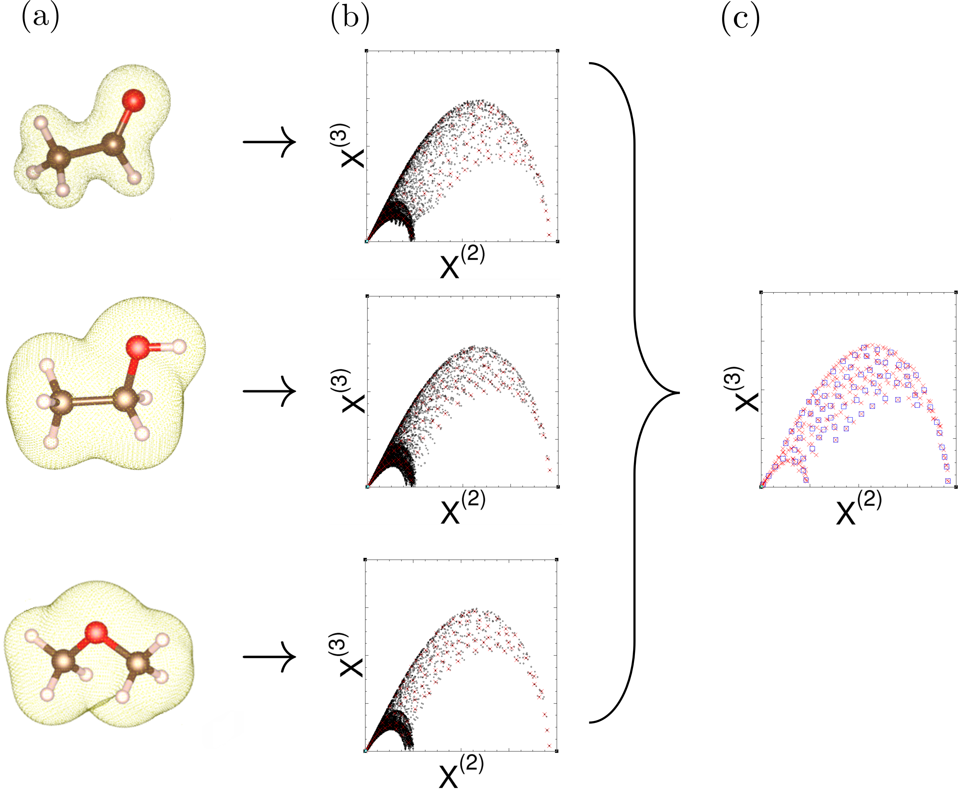
Figure 1: Data sparsification scheme for a training set consisting of three molecules, depicted in column (a). First, using the electronic density as input, we calculate the two-body descriptors $X_{n}^{(2)}(\textbf{r})$ and three-body descriptors $X_{n}^{(3)}$(r) at each real-space grid point [black dots in column (b)]. A single radial basis function is used here for visualization purposes. Next, a metric is introduced via the Gaussian kernel and representative density environments (red crosses) are chosen via k-means clustering for each training structure separately. The chosen points are concatenated and a second k-means layer selects the kernel control points $\textbf{X}^{i_{B}}$ used in Eq. (8) [blue squares in column (c)]. For more details, see Supplementary Sec. S3.

The exchange-correlation potentials provide derivative information for the ML fit as atomic forces do in MLFF, thus improving data efficiency. That is, instead of a single data point per structure for $E_{\rm xc}^{\rm RPA}$, we have additional data for $v_{\rm xc}^{\rm RPA}(\textbf{r})$ on typically $\mathcal{O}(10^{5})-\mathcal{O}(10^{6})$ grid points r. As this large amount of data cannot be handled by kernel methods, we have to employ data sparsification tools. Without loss of accuracy, the training data can be compressed dramatically by combining k-means clustering⁵⁴ with the metric induced by the Gaussian kernels (see Supplementary Sec. S3). This is illustrated in Fig. 1 using a single radial basis function, such that the descriptors can be easily visualized in 2D. Once training is complete, the computational cost of evaluating ML-RPA depends linearly on the number of kernel control points used. Further, efficient evaluation of the ML-RPA functional is achieved by extensive use of fast Fourier transforms. We find that ML-RPA is slower than standard GGA functionals by some prefactor for typical applications, but ML-RPA scales as $\mathcal{O}(N\log N)$ with system size $N$ like GGA does.⁵⁵ In comparison, non-local vdW functionals can have the same system size scaling and similar computational cost as ML-RPA,⁵⁶ whereas exact RPA is several orders of magnitude slower and has at least $\mathcal{O}(N^{3})$ scaling.^{57, 58}

3 Methods

3.1 Random-phase approximation

As the RPA includes information from unoccupied orbitals as ingredients, it sits on the fifth (highest) rung of Jacob’s ladder. In the last two decades, the RPA has been successfully employed for a multitude of problems, see Refs. 59 and 60 for reviews. In particular, the RPA is considered a “gold standard” for first-principles surface studies^{61, 62, 63} due to its seamless inclusion of vdW interactions next to the good description of covalent and metallic bonds. Combining exact exchange and a good description of dispersion interactions makes the RPA also suitable for water and ice.^{64, 65} The usual expression for the RPA exchange-correlation energy reads⁶⁶

$$E_{\rm xc}^{\rm RPA}=\text{Tr}[\ln(1-\chi_{0}V)],$$ (9)

where $\chi_{0}$ is the Kohn-Sham response function, $V$ is the Coulomb kernel, and we have used a symbolic notation for sake of brevity. As in standard Kohn-Sham DFT, one can obtain the exchange-correlation potential corresponding to the RPA exchange-correlation energy by taking the functional derivative with respect to the electronic density,

$$v_{\rm xc}^{\rm RPA}(\textbf{r})=\delta E_{\rm xc}^{\rm RPA}/\delta n(\textbf{r}).$$ (10)

Plugging in Eq. (9) and using the chain rule, one can derive the so-called optimized effective potential (OEP) equation,^{67, 68, 69, 70} symbolically

$$\chi_{0}v_{\rm xc}=G_{0}\Sigma_{\rm xc}^{G_{0}W_{0}}G_{0},$$ (11)

where $G_{0}$ is the non-interacting (Kohn-Sham) Greens-function and $\Sigma_{\rm xc}^{G_{0}W_{0}}$ is the self-energy in the $G_{0}W_{0}$ approximation. For more details on the implementations of the RPA exchange-correlation energies and the RPA-OEP method, we refer to Refs. 58 and 41, respectively.

3.2 Electronic self-consistency

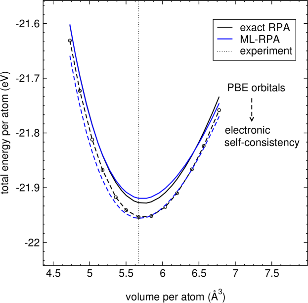
Figure 2: Energy-volume curves of bulk diamond obtained using exact RPA and ML-RPA. Full lines indicate calculations on-top of PBE orbitals, and dashed lines indicate self-consistent calculations. Self-consistent RPA reference energies are obtained using the RPA-OEP method. The dotted vertical line indicates the experimental equilibrium volume.⁷¹

Even tough the RPA-OEP method allows in principle to perform RPA calculations self-consistently,⁴¹ this procedure is seldom carried out due to the large computational overhead. A more common approach is to evaluate the RPA using orbitals from a semi-local DFT base functional (“RPA on-top of DFT”, RPA@DFT).⁷² Here, we calculate all RPA reference data using PBE as base functional (Perdew-Burke-Ernzerhof, a popular GGA functional^{11, *Perdew1997}). That is, RPA@PBE is the ground truth for ML-RPA, and we denote this ground truth in the following as “exact RPA”. Unless stated otherwise, all RPA calculations and ML-RPA calculations are thus performed non-self-consistently on-top of PBE orbitals. A ML substitute functional that reproduces only RPA@PBE would already be very useful, we reiterate that RPA@PBE is standard practice.

For the calculation of atomic forces, however, it is convenient to perform self-consistent calculations to avoid tedious non-Hellman-Feynman terms. Wherever exact RPA reference forces are required, for instance for phonon calculations, we calculate such non-Hellman-Feynman terms explicitly.⁷³ In contrast, ML-RPA can be simply run self-consistently like any semi-local density functional since the exchange-correlation potential is readily available. As a validation, we used the computationally demanding RPA-OEP method to calculate the equilibrium volume of bulk diamond self-consistently. Fig. 2 shows that ML-RPA reproduces the RPA@PBE ground truth well (solid lines). Further, ML-RPA correctly predicts a small downward shift due to electronic self-consistency (dashed lines).

We would like to emphasize that this result is not obvious, as the training set covers only PBE densities. To this point, Snyder et al.²⁸ have reported early on that electronic self-consistency can grossly deteriorate the performance of ML-DFT functionals, as self-consistency leads the functional away from its training manifold. Likewise, we observed that earlier versions of ML-RPA became inaccurate when applied self-consistently. However, we find that the current ML-RPA is very stable and reliably converges to a tight energy threshold of $10^{-8}$ eV. Key hyperparameters in this regard are the cutoff radius ($R_{\rm cut}=1.5\text{ \AA}$) and the Tikhonov regularization parameter ($t_{\rm SVD}=1.0\times 10^{-9}$, see Supplementary Sec. S2). Even atomic densities can be used as starting points, tough preconverging with PBE typically speeds up the ML-RPA self-consistency cycle. Lastly, the ML-RPA stress tensor has also been implemented via finite differences, which is useful for example for volume relaxations and the training of machine learned force fields (see Supplementary Sec. S5).

3.3 Computational details

We use the PAW code VASP (Vienna Ab Initio Simulation Package),⁷⁴ adopting the C_GW, H_GW and O_GW pseudo-potentials. All DFT and RPA calculations are performed spin-non-polarized. An energy cutoff of 600 eV is used for the plane-wave orbital basis set (ENCUT in VASP). For RPA calculations, a reduced cutoff of 400 eV is used to expand the response function $\chi_{0}$ (ENCUTGW in VASP), using a cosine window to smoothen the cutoff of the Coulomb kernel.^{72, 75} Basis set incompleteness errors are discussed in Supplementary Sec. S4. The one-center PAW contributions to the RPA exchange-correlation energy are treated on the level of Hartree-Fock, consistently for RPA and ML-RPA calculations. The good agreement of total energies in Fig. 2, rather than relative energies only, demonstrates the consistency of the ML-RPA implementation. Similar agreement is observed for all materials, with fit errors around 1 meV/electron.

4 Results

4.1 Bulk diamond

We apply our ML scheme to create an RPA substitute functional for diamond and liquid water. Following a common MLFF practice,⁴² bulk diamond training data are iteratively added from molecular dynamics (MD) simulations, using prior versions of the ML-RPA functional to create the MD trajectories. We pick 10 MD snapshots from the 8 atom supercell and 5 snapshots from the 16 atom supercell. The full ML-RPA training set is further detailed in Supplementary Sec. S4. The equilibrium lattice constant obtained by ML-RPA (3.582 Å) agrees well with the exact RPA value (3.581 Å).
Next, we calculate phonon dispersions using the finite displacement method.^{76, 77} Converged results are obtained in the large supercell limit, which is hard to achieve with exact RPA due to its unfavorable scaling behavior. Fig. 3 compares the ML-RPA phonon dispersions for different supercell sizes to exact RPA results. For contrast, phonon dispersions obtained using PBE are shown as well. For the 16 atom supercell [panel (a)], where training data are available, the ML-RPA phonon dispersion is generally in good agreement with exact RPA, though high-frequency modes are slightly underestimated. Exact RPA calculations for the larger 128 atom supercells validates the extrapolation ability of ML-RPA, as no training data are included for this supercell size. A prominent finite size effect is the closing of the gap near the K-point with respect to the smaller 16 atom cell. Further, the overbending of the LO modes reduces with increasing supercell size, which is most notable along $\Delta$ ($\Gamma$-X). These characteristic features are well reproduced with ML-RPA. The phonon dispersions obtained using exact RPA are overall in good agreement with experimental data,^{71, 78} whereas ML-RPA and PBE slightly underestimate the high-frequency modes.

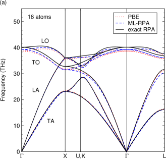
(a)

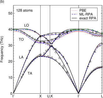
(b)

Figure 3: Phonon dispersion of diamond, calculated at the respective equilibrium lattice constants, using supercells containing (a) 16 atoms, (b) 128 atoms. Phonons obtained using exact RPA are represented as solid black lines, blue dashed lines represent ML-RPA. PBE calculations are also shown for comparison (red dotted lines). ML-RPA has training data only for the smaller supercell size [16 atoms, panel (a)]. Black and green symbols indicate experimental data from Refs. 71 and 78, respectively.

4.2 Diamond surfaces

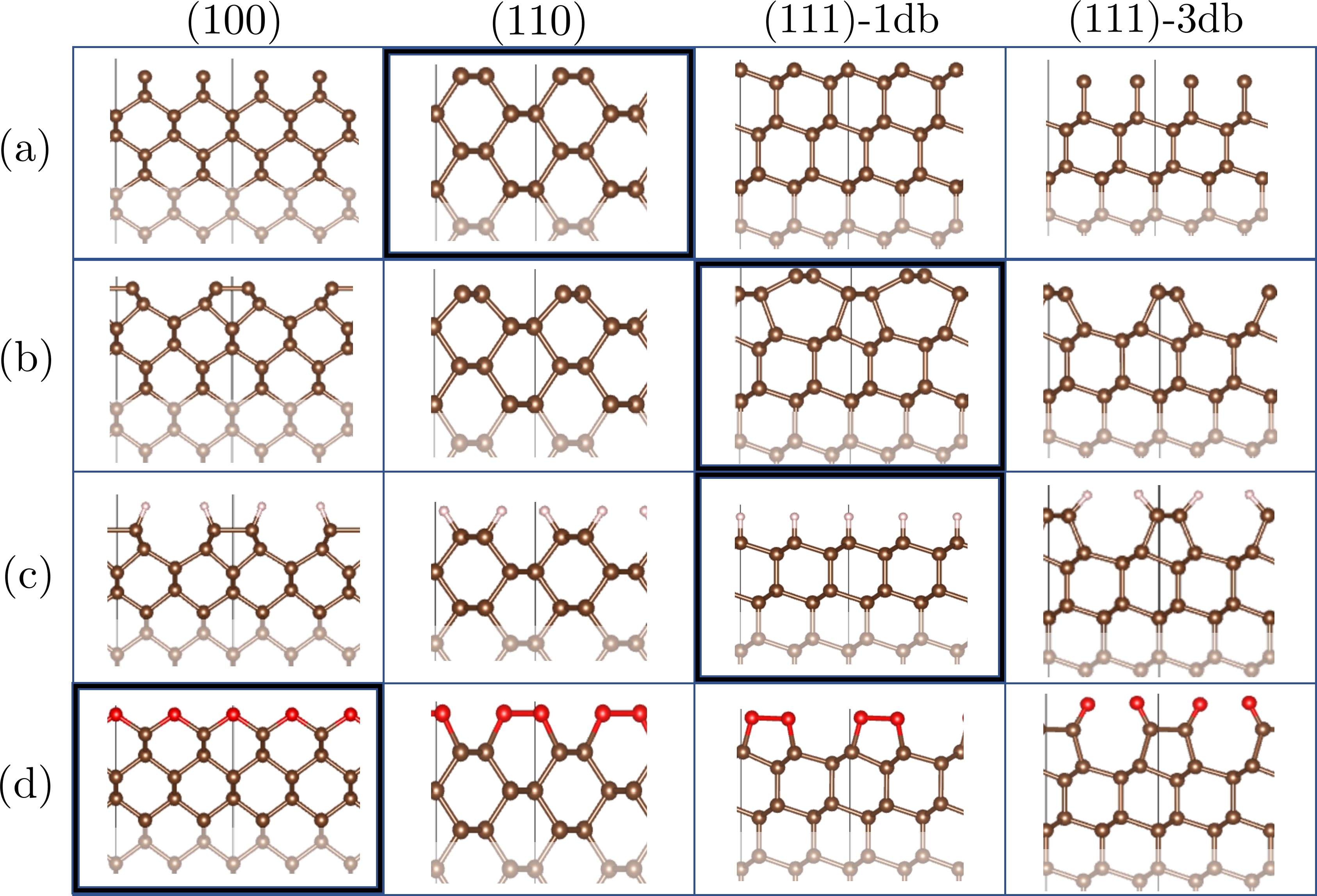
Figure 4: Side view of crystallographic diamond surfaces.⁷⁹ The $2\times 1$ simulation cells are indicated by black vertical lines, and bulk regions are indicated by faded atoms. From top to bottom: (a) clean surfaces, (b) reconstructed surfaces, (c) hydrogenated surfaces (1 ML), (d) oxygenated surfaces (1 ML). Bold edges indicate the most stable orientation for a given surface termination as predicted by exact RPA. Whereas the (111)-1db surface dereconstructs upon the chemisorption of hydrogen and oxygen,⁸⁰ the (100) surface dereconstructs only upon the chemisorption of oxygen.⁸¹ The (111)-3db surface retains the $2\times 1$ geometry throughout,⁸² and the (110) surface shows no $2\times 1$ reconstruction at all.⁸³

The advent of chemical vapor deposition (CVD) has encouraged detailed first-principles simulations of diamond surfaces. Specifically, the characterization of ideal crystallographic surfaces has proven useful for the theoretical understanding of CVD grown diamond.⁸⁴ When a diamond surface is cut, the outer surface layers can rearrange to partially eliminate the exposed dangling bonds, see Fig. 4. These reconstructions significantly change the properties of the surfaces. Further, important material properties such as electron affinity can be modified via chemisorption processes in a controlled fashion, the most important surface adsorbates being H and O.
The (100) surface is the most relevant crystallographic surface and has been thoroughly studied.^{85, 81} While the (111) surface has also received a lot of attention,^{86, 80} most studies neglect that there are two possible ways to cut this surface.^{87, 82} Namely, via the so-called glide and shuffle planes, one can expose (111) diamond surfaces with one dangling bond (1db) or three dangling bonds (3db) per surface atom, respectively. Even though the clean 1db surface is clearly more stable, 3db surfaces naturally occur in growth and etching processes. Finally, the (110) surface, which is difficult to prepare experimentally, has only recently been fully characterized.⁸⁸
In the following, we calculate diamond surface energies of formation via

$$E_{\rm surf}=(E-E_{\rm dia}/N_{\rm dia}-E_{\text{H}_{2}}/N_{\text{H}}-E_{\text{O}}/N_{\text{O}})/N_{\rm surf},$$ (12)

where $E$ is the total energy of the surface, $E_{\rm dia}$ and $E_{\text{H}_{2}}$ are the energies of bulk diamond and the $\text{H}_{2}$ molecule, and $E_{\text{O}}$ is calculated using the water monomer as reference

$$E_{\text{O}}=E_{\text{H}_{2}\text{O}}-E_{\text{H}_{2}}.$$ (13)

Vibrational contributions to the formation energies due to zero-point motion are neglected. Diamond surface calculations are performed in $2\times 1$ supercells using symmetric slabs. We use 18 surface layers for the (111)-1db surface and 16 layers for the rest. This assures convergence of the surface formation energies to better than 10 meV accuracy.^{86, 83} The surface geometries were obtained using the PBE functional, further details are given in Supplementary Sec. S4.
RPA formation energies of diamond surfaces are collected in Table 1. (100) and (111)-1db surfaces were included in training, whereas (110) and (111)-3db surfaces are left as independent tests for ML-RPA. For all surface terminations studied, ML-RPA correctly predicts the most stable surface orientation (underlined values). For example, of the clean surfaces (as cut), both RPA and ML-RPA predict the order (110) $<$ (111)-1db $<$ (100) $<$ (111)-3db, which can be qualitatively understood via coordination of the surface atoms.⁸⁶ Note that the (111)-3db surface becomes increasingly competitive with the (111)-1db surface as more dangling bonds are eliminated via reconstruction (-1 db) and chemisorption (-2 db for H, -3 db for O).

Including calculations of metastable surfaces (see Supplementary Sec. S4), we have assembled a database of 28 RPA surface formation energies in total. It is interesting to use these data as benchmark for other exchange-correlation functionals. Table 2 shows that all functionals including ML-RPA tend to predict smaller formation energies than exact RPA (negative mean relative errors). In terms of accuracy, ML-RPA performs very well, with a mean absolute error of 70 meV per surface atom. Surface energies predicted by the meta-GGA functional SCAN as well as the vdW functionals PBE+TS and SCAN+rVV10 are also in very good agreement with exact RPA, with mean absolute errors slightly larger than ML-RPA. Finally, we comment again on the stability of electronic self-consistancy. Going from ML-RPA@PBE to self-consistent ML-RPA, individual surface energies change by 60 meV per surface atom or less, and the mean absolute error of self-consistent ML-RPA (compared to exact RPA@PBE) is only 80 meV per surface atom. Thus, the accuracy of ML-RPA is not significantly diminished by electronic self-consistency.

Table 1: RPA energies of formation for diamond surfaces, calculated via Eq. (12) (in eV per surface atom). The most stable surface orientation for a given surface termination is underlined, and surfaces included in the ML-RPA training set are marked by asterisks. Surface calculations are performed in $2\times 1$ supercells, with geometries illustrated in Fig. 4.

	$(100)^{*}$		(110)		(111)-1db∗		(111)-3db
	exact	ML	exact	ML	exact	ML	exact	ML
clean	3.66	3.57	2.09	1.95	2.69	2.52	4.37	4.37
reconstructed	$2.08$	2.03	1.70	1.59	1.41	1.34	2.70	2.56
+H (1 ML)	$0.20$	0.11	-0.11	-0.12	-0.19	-0.24	0.17	0.11
+O (1 ML)	1.99	1.91	3.23	3.21	$2.99$	2.94	2.90	2.79
∗included in the ML-RPA training set

Table 2: Surface formation energies from different exchange-correlation functionals compared to values from exact RPA. Mean signed error (MSE), mean absolute error (MAE) and maximum absolute error (MAX) are given in eV per surface atom. Averages are over 28 diamond surfaces of which 16 are in the ML-RPA training set, see Supplementary Section D.

	MSE	MAE	MAX
LDA	-0.06	0.14	0.34
PBEsol	-0.10	0.12	0.33
PBE	-0.19	0.19	0.39
RPBE	-0.23	0.24	0.44
PBE+TS	-0.01	0.08	0.25
RPBE+D3(BJ)	-0.09	0.12	0.48
optB88-vdW	-0.19	0.19	0.62
rev-vdW-DF2	-0.13	0.14	0.52
rVV10	-0.18	0.18	0.57
SCAN	-0.08	0.11	0.25
SCAN+rVV10	-0.03	0.10	0.24
ML-RPA	-0.07	0.07	0.18

4.3 Liquid water

Water with its many anomalies is both an important and challenging system for first-principles molecular dynamics simulations.⁸⁹ The role of the exchange-correlation functional for the description of liquid water and ice has been studied extensively.^{64, 90, 91, 92} This has made water an interesting target for several recent MLFF^{93, 94, 65} and ML-DFT^{50, 24} approaches.
In particular, Yao and Kanai⁶⁵ used MLFF to perform RPA-level calculations for liquid water with the inclusion of nuclear quantum effects. They showed that the RPA can well reproduce experimental data for numerous water properties at different temperatures. Due to the small mass of the hydrogen atom, the oxygen-hydrogen radial distribution function (RDF) and especially the hydrogen-hydrogen RDF are significantly altered by nuclear quantum effects. Namely, classical MD predicts an oxygen-hydrogen RDF that is overstructured compared to experimental data, and even more so for the hydrogen-hydrogen RDF. In contrast, the oxygen-oxygen RDF is far less affected, especially for higher temperatures.

To perform calculations on liquid water, we add 32 liquid water structures containing 8 water molecules to the ML-RPA training set, as well as 39 structures using larger supercells (31 or 32 water molecules). The structures are again sampled from MD trajectories created by earlier ML-RPA versions. In addition, the ML-RPA training set contains 6 structures sampling the water monomer.

Accurate determination of the water RDFs require long MD simulations that are computationally expensive even without nuclear quantum corrections. Thus, we perform classical MDs using 64 water molecules and speed them up by combining ML-RPA with MLFF. That is, we train a machine learning force field “on-the-fly”^{95, 36} using the energies and forces predicted by ML-RPA. In order to obtain an RPA reference for the radial distribution function, we also train an MLFF directly on exact RPA energies and forces (RPA-MLFF). The RPA-MLFF training set contains all water structures from the ML-RPA training set plus 30 additional structures containing 32 molecules. To validate our machine learning force fields, we also trained on-the-fly MLFFs for the vdW functionals RPBE+D3(BJ)^{96, 97} and PBE+TS.⁹⁸ Further details of the MLFF setups are given in Supplementary Sec. S5.

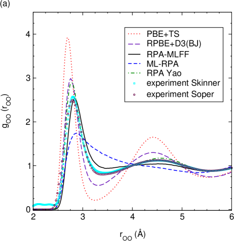
(a)

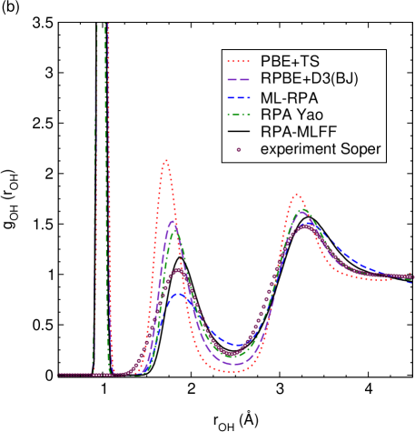
(b)

Figure 5: Partial radial distribution functions of liquid water at ambient conditions ($\text{T}=300\text{ K}$, $\rho=1\text{ g/cm}^{3}$), details of the MD simulations are given in Supplementary Sec. S5. (a) oxygen-oxygen radial distribution function, (b) oxygen-hydrogen radial distribution function. RPA results from Yao and Kanai are extracted from Ref. 65, experimental data are taken from Refs. 99, 100. See text for a discussion of nuclear quantum effects.

Fig 5 shows the oxygen-oxygen RDF, $g_{\rm OO}$, and oxygen-hydrogen RDF, $g_{\rm OH}$, at ambient conditions. First, we note that the RDFs obtained from PBE+TS and RPBE+D3(BJ) are in good agreement with respective literature results^{101, 102} (for PBE+TS, we compared the RDF at T = 330 K, not shown). The PBE+TS RDF is clearly overstructured compared to experimental data. The water structure is “too tetragonal”, even more so when the TS vdW correction is not included, see Ref. 101. The RPBE+D3(BJ) RDF is in better agreement with experiment, but is still somewhat overstructured. This is a specific effect of the Becke-Johnson (BJ) damping, that is, the RPBE+D3(0) RDF (using zero damping) is closer to experiment (see Ref. 102). Next, the RDFs predicted by RPA-MLFF are less structured than the RPA references of Yao and Kanai, compare the first peaks and minima of both $g_{\rm OO}$ and $g_{\rm OH}$. This discrepancy is possibly due to technical convergence of either RPA calculation, in particular, basis set incompleteness errors. The fact that RPA-MLFF closely reproduces the first experimental peak height of $g_{\rm OO}$ is arguably accidental, since nuclear quantum effects are not included. For $g_{\rm OH}$, however, the result of Yao and Kanai is still more structured than experiment even with nuclear quantum effects included (see Fig. 1 in Ref. 65), indicating that our RPA reference is potentially more accurate.

That said, overall both RPA reference results agree well with experimental data. Turning to the water structure predicted by ML-RPA, there are some clear discrepancies from both RPA references. The first peak of $g_{\rm OO}$ is smaller in height, and the second peak is completely missing. The $g_{\rm OH}$ predicted by ML-RPA is also somewhat less structured than the RPA references, but the overall agreement is better than for $g_{\rm OO}$. Importantly, the discrepancies are mainly due to the actual ML-RPA density functional, since the on-the-fly MLFF is very accurate (see Supplementary Sec. S5). Specifically, atomic forces for all MLFFs trained here exhibit an root mean square error of roughly $30\text{ meV \AA}^{-1}$, whereas the respective force errors for liquid water due to ML-RPA are roughly $90\text{ meV \AA}^{-1}$. It is also important to point out that the RPA-MLFF is a single-purpose force field, trained specifically to simulate liquid water in the bulk (and the water monomer). In contrast, the ML-RPA functional is not limited in this way as will be demonstrated in the following section.

4.4 Smaller water clusters

Table 3: Ground state properties of the $\text{H}_{2}\text{O}$ dimer. Dimer binding energies, $E_{\rm b}^{\rm dim}=-E[(\text{H}_{2}\text{O})_{2}]+2E[\text{H}_{2}\text{O}]$, are given in eV. Equilibrium bond lengths $d_{\rm OO}^{\rm dim}$ and $d_{\rm OH}^{\rm dim}$ are given in Å. All calculations are performed fully self-consistently.

	$E_{\rm b}^{\rm dim}$	$d_{\rm OO}^{\rm dim}$	$d_{\rm OH}^{\rm dim}$
LDA	0.39	2.72	1.73
PBEsol	0.27	2.80	1.82
PBE	0.23	2.88	1.91
RPBE	0.17	3.02	2.04
PBE+TS	0.24	2.89	1.92
RPBE+D3(BJ)	0.21	2.94	1.97
optB88-vdW	0.22	2.90	1.93
rev-vdW-DF2	0.23	2.89	1.92
rVV10	0.25	2.88	1.90
SCAN	0.25	2.84	1.88
SCAN+rVV10	0.26	2.84	1.88
ML-RPA	0.18	3.07	2.10
RPA-MLFF	0.21	3.28	2.30
CCSD(T)103	0.22	2.91	1.96

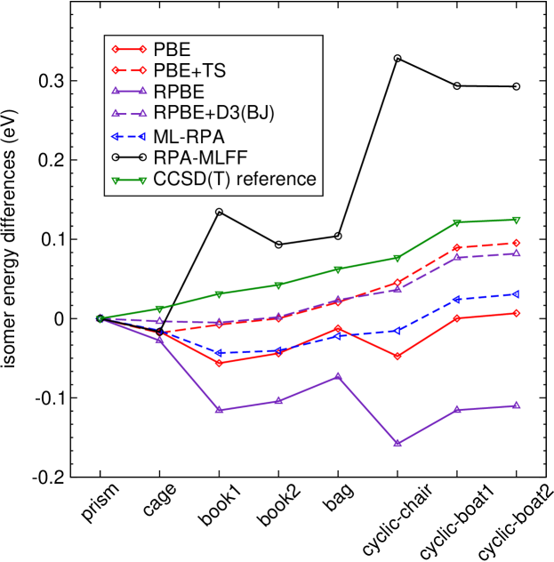
Figure 6: Binding energy differences of eight $\text{H}_{2}\text{O}$ hexamers. Geometries and CCSD(T) reference data are taken from Ref. 104. The vdW functionals PS+TS and RPBE+D3(BJ) largely correct the errors of their respective GGA base functionals, see also Supplementary Sec. S6. Lines drawn are only guides to the eye.

An important $\text{H}_{2}\text{O}$ benchmark is the performance for smaller water clusters.⁹¹ Already the simple $\text{H}_{2}\text{O}$ dimer gives a predictive measure of the strength of a hydrogen bond in liquid water. Table 3 shows that ML-RPA predicts a somewhat underbound dimer, consistent with the understructured liquid. Going to larger clusters, the water hexamers present a difficult challenge for DFT, as three-dimensional structures (“prism”,”cage”,”bag”) compete energetically with two-dimensional ones (“book”,”chair”,”boat”). Fig. 6 shows that ML-RPA erroneously predicts two-dimensional structures to be most stable, as do all GGA functionals (see also Supplementary Sec. S6). LDA and the SCAN meta-GGA functional perform well in this regard, but overbind the dimer, compare Table 3. All vdW functionals tested give excellent results for both the dimer as well as the hexamers. This confirms the critical role that vdW interactions play for the structure of water.^{91, 93} Further, RPA-MLFF clearly fails for water clusters, but we reiterate that it has been trained only for liquid water in the bulk. The fact that RPA-MLFF extrapolates is substantiated by large Bayesian error predictions: compared to typical bulk water configurations, the maximum force Bayesian error is three times as large for the hexamers and five times as large for the dimer.

Finally, we investigated cubic ice, specifically, the $\rm I_{c}$(a) proton-ordered ice phase as described in Ref. 64. The equilibrium volume predicted by RPA-MLFF is $\text{32.3 \AA}^{3}{\text{ per H}}_{2}{\text{O}}$, in good agreement with the $\text{32.6 \AA}^{3}{\text{ per H}}_{2}{\text{O}}$ obtained using exact RPA. The ML-RPA equilibrium volume is somewhat smaller ($\text{31.2 \AA}^{3}{\text{ per H}}_{2}{\text{O}}$). For comparison, the equilibrium volumes predicted by PBE and PBE+TS are $\text{30.2 \AA}^{3}{\text{ per H}}_{2}{\text{O}}$ and $\text{30.0 \AA}^{3}{\text{ per H}}_{2}{\text{O}}$, respectively. In summation, ML-RPA provides a consistent but somewhat inaccurate description of water and ice. The fact that ML-RPA misses the second $g_{\rm OO}$ maximum, underbinds the water dimer, and provides a PBE-like description of the water hexamers and cubic ice strongly indicates that the current ML-RPA misses some crucial non-local interactions. This is likely connected to the rather small cutoff radius used here for ML-RPA ($R_{\rm cut}=1.5\text{ \AA}$). However, increasing the cutoff is not beneficial for the current ML-RPA, our tests indicate that this diminishes ML-RPA accuracy (not shown).

4.5 Homogeneous electron gas

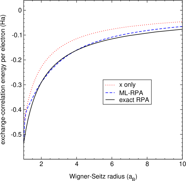
Figure 7: Application of ML-RPA to the homogeneous electron gas. Exact RPA results were taken from Ref. 75, the exchange only approximation $\varepsilon_{\rm x,HEG}$ is also shown for comparison. No HEG data were added to the ML-RPA training set.

To challenge the extrapolation abilities of our ML-RPA functional, we apply it to the homogeneous electron gas (HEG). The HEG constitutes an “appropriate norm”, that is an important theoretical limit that density functionals should fulfill. Due to symmetry, the HEG is completely characterized by the electron density $n$, or equivalently the Wigner-Seitz radius $r_{\rm s}=(3/4\pi n)^{1/3}$. Starting with LDA, many successful exchange-correlation functionals are designed such that they describe the HEG exactly, but this is not the case for the present ML-RPA functional. It is important to point out that the ground truth here is the exchange-correlation energy per electron as given by exact RPA. As the RPA is itself an approximation, $\varepsilon_{\rm xc,HEG}^{\rm RPA}$ differs from the usual LDA which is based on exact numerical data from Quantum Monte Carlo calculations.¹⁰⁵ Figure 7 shows that ML-RPA for intermediate densities ($r_{\rm s}\sim 2-5$) closely follows the exact RPA reference. Since this is the range of physical densities, ML-RPA seems to have learned the HEG indirectly from diamond and water data. Still, this excellent agreement comes somewhat surprising considering that no HEG data were explicitly added to the ML-RPA training set. Furthermore, for small densities ($r_{\rm s}\gtrsim 5$), ML-RPA is slightly less accurate but still well behaved. Finally, for large densities ($r_{\rm s}\lesssim 2$), ML-RPA develops an unphysical kink. This indicates the presence of an “extrapolation hole”, that is, the complete lack of training data can cause erratic behavior.

5 Discussion

The LDA and different GGA functionals differ in the strength of their respective enhancement factors. This results, for example, in the following trend for cohesive energies of solids

$$\text{LDA}>\text{PBEsol}>\text{PBE}>\text{RPBE}.$$ (14)

The same trend is also manifest for surface formation energies and molecular adsorption energies.⁶¹ As different enhancement strengths fit better for different physical properties, this leads to a well-known trade-off for GGA functionals. This trade-off is visible also in the current study: LDA and PBEsol give better diamond surface energies (Table 2). PBE and RPBE perform better for the water dimer (Table 3), but the trend is reversed for the hexamer puzzle (Supplementary Sec. S6). This means that no GGA functional can give a completely satisfactory description of liquid water and ice, see also Ref. 91 for a more in-depth discussion. We have demonstrated that the non-local gradient approximation used in our ML-RPA model can overcome the GGA trade-off to some extend. While ML-RPA does not exceed a GGA-level description of liquid water, it clearly outperforms all GGA functionals for the diamond surface benchmark.

Traditional routes beyond GGA are metaGGA and hybrid functionals on the one hand, and vdW functionals on the other hand. The RPA itself can be considered as the “gold standard” of vdW functionals.¹⁰⁶ Different vdW functionals tested here generally outperform their respective semi-local DFT base functionals, though the improvement is not always consistent. For example, the rVV10 vdW correction slightly increases the surface energies of the pristine SCAN functional, achieving good agreement with exact RPA (Table 2, Ref. 62). On the other hand, SCAN already slightly overbinds the water dimer and gives a somewhat overstructured liquid. Thus, it is plausible that additional binding in the form of rVV10 can only deteriorate the performance of SCAN for water (Supplementary Sec. S6, Ref. 107). We reason that the rather small cutoff radius adapted here for ML-RPA is not sufficient to capture the full non-locality that is required for a complete description of liquid water (ML-RPA uses a cutoff radius of 1.5 Å, whereas RPA-MLFF uses a larger cutoff of 6.0 Å). However, simply increasing the cutoff radius is not an option with the current implementation and training database. We repeat that our tests show that a larger cutoff would diminish fit accuracy. Future work could instead focus on the construction of explicitly long-range descriptors as present in non-local vdW functionals or in recent extensions of MLFF frameworks.¹⁰⁸

Finally, a common problem of ML techniques is extrapolation, that is, one can only expect good performance if applications are similar enough to the respective training sets. Here, this point was demonstrated by the poor performance of RPA-MLFF for water clusters (RPA-MLFF has been trained only for bulk water and the water monomer). In contrast, ML-RPA gives consistent if inaccurate predictions, though it has less water training data. We speculate that this is due to ML-RPA descriptors being much more compact, which makes extrapolation more manageable. Specifically, here we used 8 density descriptors for ML-RPA versus 408 atomic descriptors for RPA-MLFF (204 for both O and H). It is worth pointing out that this difference will be exacerbated when more chemical species have to be described at the same time. That is, the number of descriptors in MLFF schemes generally scales unfavorably with the number of chemical species, whereas the density descriptors used for ML-RPA do not depend explicitly on atom type. On the other side, RPA-MLFF is in the present implementation undeniable superior in terms of raw fit accuracy. ML-RPA and RPA-MLFF thus strike different balances between model flexibility and universality.

When pushed even further outside of its training set, however, ML-RPA eventually extrapolates as well as demonstrated for the homogeneous electron gas. The obvious but costly solution to the extrapolation problem is the construction of ever larger training databases. A more elegant alternative would be to enforce ML-RPA to obey known exact constraints. Exact constraints have been used in the past to construct successful functionals such as the SCAN functional (“Strongly constrained and appropriately normed”).¹⁴ Recently, there have been some promising efforts to incorporate exact constraints also into machine learned density functionals.^{109, 24, 110, 52}

6 Conclusion and Outlook

In this work we have machine learned a substitute density functional based on the random-phase approximation. The ingredients of ML-RPA are density descriptors constructed analogously to the two- and three-body descriptors used for machine learned force fields. These ingredients can be considered as non-local extensions of the local density and its gradient. As a first application, we have constructed an ML-RPA functional for diamond and liquid water. We have demonstrated how such a functional can be used to enable RPA calculations at a larger scale. For a data set of 28 diamond surfaces, ML-RPA surpasses all tested GGA functionals in terms of accuracy and reaches the level of state-of-the-art vdW functionals. For liquid water, ML-RPA is less accurate and falls back to a GGA-level description, which we traced back to an insufficient description of non-local interactions.

Our ML-RPA scheme was demonstrated to learn fairly quickly from small amounts of exact RPA data, with the entire data base consisting of less than 200 structures. We credit this data efficiency to the inclusion of derivative information in the form of RPA exchange-correlation potentials, which are obtained via the optimized effective potential method. This is in close analogy to fitting atomic forces in MLFF. Generally, the tasks of machine learning atomic force fields and machine learning density functionals are closely related. We hope to see continued exchange of concepts and techniques, as we believe that both fields can benefit immensely from such a “cross-fertilization” of ideas.

Finally, our machine learning method using optimized effective potentials is general and not limited to the random-phase approximation. For example, beyond RPA theories can be constructed by including vertex correction to the screened Coulomb interaction and/or self energy. One can also envision to extract high accuracy exchange-correlation potentials from accurate coupled-cluster densities via Kohn-Sham inversion. Our method can also be applied to learn hybrid functionals, where large databases can be obtained more easily, thus facilitating large-scale hybrid functional simulations.

Computation time at the Vienna Scientific Cluster (VSC) is gratefully acknowledged. The authors thank K. Burke as well as K. Bystrom and B. Kozinsky for fruitful discussions.

Author declarations

Conflict of interest

The authors declare no competing interests.

Data availability

The ML-RPA training data is freely available at https://doi.org/10.25365/phaidra.418.

Analytical proof of Eqs. (3) and (5) (S1), analytical expressions for the ML-RPA exchange-correlation potentials (S2), details of our data sparsification scheme (S3), training details for ML-RPA (S4) and RPA-MLFF (S5), water hexamer benchmark for more DFT functionals (S6).

References

- Burke 2012 Burke, K. Perspective on density functional theory. The Journal of Chemical Physics 2012, 136, 150901
- Medvedev et al. 2017 Medvedev, M. G.; Bushmarinov, I. S.; Sun, J.; Perdew, J. P.; Lyssenko, K. A. Density functional theory is straying from the path toward the exact functional. Science 2017, 355, 49–52
- Hohenberg and Kohn 1964 Hohenberg, P.; Kohn, W. Inhomogeneous Electron Gas. Phys. Rev. 1964, 136, B864–B871
- Kohn 1999 Kohn, W. Nobel Lecture: Electronic structure of matter—wave functions and density functionals. Reviews of Modern Physics 1999, 71, 1253–1266
- Kohn and Sham 1965 Kohn, W.; Sham, L. J. Self-Consistent Equations Including Exchange and Correlation Effects. Phys. Rev. 1965, 140, A1133–A1138
- Perdew and Schmidt 2001 Perdew, J. P.; Schmidt, K. Jacob’s ladder of density functional approximations for the exchange-correlation energy. AIP Conference Proceedings 2001, 577, 1–20
- Seidl et al. 1996 Seidl, A.; Görling, A.; Vogl, P.; Majewski, J. A.; Levy, M. Generalized Kohn-Sham schemes and the band-gap problem. Physical Review B 1996, 53, 3764–3774
- Dion et al. 2004 Dion, M.; Rydberg, H.; Schröder, E.; Langreth, D. C.; Lundqvist, B. I. Van der Waals Density Functional for General Geometries. Physical Review Letters 2004, 92, 246401
- Dion et al. 2005 Dion, M.; Rydberg, H.; Schröder, E.; Langreth, D. C.; Lundqvist, B. I. Erratum: Van der Waals Density Functional for General Geometries [Phys. Rev. Lett. 92, 246401 (2004)]. Physical Review Letters 2005, 95, 109902
- Berland et al. 2015 Berland, K.; Cooper, V. R.; Lee, K.; Schröder, E.; Thonhauser, T.; Hyldgaard, P.; Lundqvist, B. I. van der Waals forces in density functional theory: a review of the vdW-DF method. Reports on Progress in Physics 2015, 78, 066501
- Perdew et al. 1996 Perdew, J. P.; Burke, K.; Ernzerhof, M. Generalized Gradient Approximation Made Simple. Phys. Rev. Lett. 1996, 77, 3865–3868
- Perdew et al. 1997 Perdew, J. P.; Burke, K.; Ernzerhof, M. Generalized Gradient Approximation Made Simple [Phys. Rev. Lett. 77, 3865 (1996)]. Phys. Rev. Lett. 1997, 78, 1396–1396
- Perdew et al. 1996 Perdew, J. P.; Ernzerhof, M.; Burke, K. Rationale for mixing exact exchange with density functional approximations. The Journal of Chemical Physics 1996, 105, 9982–9985
- Sun et al. 2015 Sun, J.; Ruzsinszky, A.; Perdew, J. P. Strongly Constrained and Appropriately Normed Semilocal Density Functional. Phys. Rev. Lett. 2015, 115, 036402
- Becke 1988 Becke, A. D. Density-functional exchange-energy approximation with correct asymptotic behavior. Physical Review A 1988, 38, 3098–3100
- Lee et al. 1988 Lee, C.; Yang, W.; Parr, R. G. Development of the Colle-Salvetti correlation-energy formula into a functional of the electron density. Physical Review B 1988, 37, 785–789
- Becke 1993 Becke, A. D. Density-functional thermochemistry. III. The role of exact exchange. The Journal of Chemical Physics 1993, 98, 5648–5652
- Zhao and Truhlar 2007 Zhao, Y.; Truhlar, D. G. The M06 suite of density functionals for main group thermochemistry, thermochemical kinetics, noncovalent interactions, excited states, and transition elements: two new functionals and systematic testing of four M06-class functionals and 12 other functionals. Theoretical Chemistry Accounts 2007, 120, 215–241
- Stephens et al. 1994 Stephens, P. J.; Devlin, F. J.; Chabalowski, C. F.; Frisch, M. J. Ab Initio Calculation of Vibrational Absorption and Circular Dichroism Spectra Using Density Functional Force Fields. The Journal of Physical Chemistry 1994, 98, 11623–11627
- Paier et al. 2007 Paier, J.; Marsman, M.; Kresse, G. Why does the B3LYP hybrid functional fail for metals? The Journal of Chemical Physics 2007, 127, 024103
- Cramer and Truhlar 2009 Cramer, C. J.; Truhlar, D. G. Density functional theory for transition metals and transition metal chemistry. Physical Chemistry Chemical Physics 2009, 11, 10757
- Nagai et al. 2020 Nagai, R.; Akashi, R.; Sugino, O. Completing density functional theory by machine learning hidden messages from molecules. npj Computational Materials 2020, 6, 1–8
- Bogojeski et al. 2020 Bogojeski, M.; Vogt-Maranto, L.; Tuckerman, M. E.; Müller, K.-R.; Burke, K. Quantum chemical accuracy from density functional approximations via machine learning. Nature Communications 2020, 11, 1–11
- Dick and Fernandez-Serra 2021 Dick, S.; Fernandez-Serra, M. Highly accurate and constrained density functional obtained with differentiable programming. Physical Review B 2021, 104, l161109
- Kirkpatrick et al. 2021 Kirkpatrick, J.; McMorrow, B.; Turban, D. H. P.; Gaunt, A. L.; Spencer, J. S.; Matthews, A. G. D. G.; Obika, A.; Thiry, L.; Fortunato, M.; Pfau, D.; Castellanos, L. R.; Petersen, S.; Nelson, A. W. R.; Kohli, P.; Mori-Sánchez, P.; Hassabis, D.; Cohen, A. J. Pushing the frontiers of density functionals by solving the fractional electron problem. Science 2021, 374, 1385–1389
- Tozer et al. 1996 Tozer, D. J.; Ingamells, V. E.; Handy, N. C. Exchange-correlation potentials. The Journal of Chemical Physics 1996, 105, 9200–9213
- Hamprecht et al. 1998 Hamprecht, F. A.; Cohen, A. J.; Tozer, D. J.; Handy, N. C. Development and assessment of new exchange-correlation functionals. The Journal of Chemical Physics 1998, 109, 6264–6271
- Snyder et al. 2012 Snyder, J. C.; Rupp, M.; Hansen, K.; Müller, K.-R.; Burke, K. Finding Density Functionals with Machine Learning. Phys. Rev. Lett. 2012, 108, 253002
- Li et al. 2015 Li, L.; Snyder, J. C.; Pelaschier, I. M.; Huang, J.; Niranjan, U.-N.; Duncan, P.; Rupp, M.; Müller, K.-R.; Burke, K. Understanding machine-learned density functionals. International Journal of Quantum Chemistry 2015, 116, 819–833
- Brockherde et al. 2017 Brockherde, F.; Vogt, L.; Li, L.; Tuckerman, M. E.; Burke, K.; Müller, K.-R. Bypassing the Kohn-Sham equations with machine learning. Nature Communications 2017, 8, 1–10
- Kalita et al. 2021 Kalita, B.; Li, L.; McCarty, R. J.; Burke, K. Learning to Approximate Density Functionals. Accounts of Chemical Research 2021, 54, 818–826
- Schmidt et al. 2019 Schmidt, J.; Marques, M. R. G.; Botti, S.; Marques, M. A. L. Recent advances and applications of machine learning in solid-state materials science. npj Computational Materials 2019, 5, 1–36
- Bartók et al. 2013 Bartók, A. P.; Kondor, R.; Csányi, G. On representing chemical environments. Physical Review B 2013, 87, 184115
- Bartók et al. 2013 Bartók, A. P.; Kondor, R.; Csányi, G. Publisher’s Note: On representing chemical environments [Phys. Rev. B 87, 184115 (2013)]. Physical Review B 2013, 87, 219902
- Bartók et al. 2017 Bartók, A. P.; Kondor, R.; Csányi, G. Erratum: On representing chemical environments [Phys. Rev. B 87, 184115 (2013)]. Physical Review B 2017, 96, 019902
- Jinnouchi et al. 2019 Jinnouchi, R.; Karsai, F.; Kresse, G. On-the-fly machine learning force field generation: Application to melting points. Physical Review B 2019, 100, 014105
- Chmiela et al. 2017 Chmiela, S.; Tkatchenko, A.; Sauceda, H. E.; Poltavsky, I.; Schütt, K. T.; Müller, K.-R. Machine learning of accurate energy-conserving molecular force fields. Science Advances 2017, 3, e1603015
- Nagai et al. 2018 Nagai, R.; Akashi, R.; Sasaki, S.; Tsuneyuki, S. Neural-network Kohn-Sham exchange-correlation potential and its out-of-training transferability. The Journal of Chemical Physics 2018, 148, 241737
- Zhou et al. 2019 Zhou, Y.; Wu, J.; Chen, S.; Chen, G. Toward the Exact Exchange–Correlation Potential: A Three-Dimensional Convolutional Neural Network Construct. The Journal of Physical Chemistry Letters 2019, 10, 7264–7269
- Schmidt et al. 2019 Schmidt, J.; Benavides-Riveros, C. L.; Marques, M. A. L. Machine Learning the Physical Nonlocal Exchange–Correlation Functional of Density-Functional Theory. The Journal of Physical Chemistry Letters 2019, 10, 6425–6431
- Riemelmoser et al. 2021 Riemelmoser, S.; Kaltak, M.; Kresse, G. Optimized effective potentials from the random-phase approximation: Accuracy of the quasiparticle approximation. The Journal of Chemical Physics 2021, 154, 154103
- Behler and Parrinello 2007 Behler, J.; Parrinello, M. Generalized Neural-Network Representation of High-Dimensional Potential-Energy Surfaces. Physical Review Letters 2007, 98, 146401
- Gunnarsson et al. 1979 Gunnarsson, O.; Jonson, M.; Lundqvist, B. I. Descriptions of exchange and correlation effects in inhomogeneous electron systems. Physical Review B 1979, 20, 3136–3164
- Jinnouchi et al. 2020 Jinnouchi, R.; Karsai, F.; Verdi, C.; Asahi, R.; Kresse, G. Descriptors representing two- and three-body atomic distributions and their effects on the accuracy of machine-learned inter-atomic potentials. The Journal of Chemical Physics 2020, 152, 234102
- Lei and Medford 2019 Lei, X.; Medford, A. J. Design and analysis of machine learning exchange-correlation functionals via rotationally invariant convolutional descriptors. Physical Review Materials 2019, 3, 063801
- Shapeev 2016 Shapeev, A. V. Moment Tensor Potentials: A Class of Systematically Improvable Interatomic Potentials. Multiscale Modeling & Simulation 2016, 14, 1153–1173
- Drautz 2019 Drautz, R. Atomic cluster expansion for accurate and transferable interatomic potentials. Physical Review B 2019, 99, 014104
- Drautz 2019 Drautz, R. Erratum: Atomic cluster expansion for accurate and transferable interatomic potentials [Phys. Rev. B 99, 014104 (2019)]. Physical Review B 2019, 100, 249901
- Grisafi et al. 2018 Grisafi, A.; Fabrizio, A.; Meyer, B.; Wilkins, D. M.; Corminboeuf, C.; Ceriotti, M. Transferable Machine-Learning Model of the Electron Density. ACS Central Science 2018, 5, 57–64
- Margraf and Reuter 2021 Margraf, J. T.; Reuter, K. Pure non-local machine-learned density functional theory for electron correlation. Nature Communications 2021, 12, 1–7
- Dick and Fernandez-Serra 2020 Dick, S.; Fernandez-Serra, M. Machine learning accurate exchange and correlation functionals of the electronic density. Nature Communications 2020, 11, 1–10
- Bystrom and Kozinsky 2022 Bystrom, K.; Kozinsky, B. CIDER: An Expressive, Nonlocal Feature Set for Machine Learning Density Functionals with Exact Constraints. Journal of Chemical Theory and Computation 2022, 18, 2180–2192
- Chen et al. 2020 Chen, Y.; Zhang, L.; Wang, H.; E, W. DeePKS: A Comprehensive Data-Driven Approach toward Chemically Accurate Density Functional Theory. Journal of Chemical Theory and Computation 2020, 17, 170–181
- Arthur and Vassilvitskii 2006 Arthur, D.; Vassilvitskii, S. k-means++: The Advantages of Careful Seeding; Technical Report 2006-13, 2006
- White and Bird 1994 White, J. A.; Bird, D. M. Implementation of gradient-corrected exchange-correlation potentials in Car-Parrinello total-energy calculations. Phys. Rev. B 1994, 50, 4954–4957
- Román-Pérez and Soler 2009 Román-Pérez, G.; Soler, J. M. Efficient Implementation of a van der Waals Density Functional: Application to Double-Wall Carbon Nanotubes. Physical Review Letters 2009, 103, 096102
- Rojas et al. 1995 Rojas, H. N.; Godby, R. W.; Needs, R. J. Space-Time Method for Ab Initio Calculations of Self-Energies and Dielectric Response Functions of Solids. Phys. Rev. Lett. 1995, 74, 1827–1830
- Kaltak et al. 2014 Kaltak, M.; Klimeš, J.; Kresse, G. Low Scaling Algorithms for the Random Phase Approximation: Imaginary Time and Laplace Transformations. Journal of Chemical Theory and Computation 2014, 10, 2498–2507
- Ren et al. 2012 Ren, X.; Rinke, P.; Joas, C.; Scheffler, M. Random-phase approximation and its applications in computational chemistry and materials science. Journal of Materials Science 2012, 47, 7447–7471
- Eshuis et al. 2012 Eshuis, H.; Bates, J. E.; Furche, F. Electron correlation methods based on the random phase approximation. Theoretical Chemistry Accounts 2012, 131, 1–18
- Schimka et al. 2010 Schimka, L.; Harl, J.; Stroppa, A.; Grüneis, A.; Marsman, M.; Mittendorfer, F.; Kresse, G. Accurate surface and adsorption energies from many-body perturbation theory. Nature Materials 2010, 9, 741–744
- Patra et al. 2017 Patra, A.; Bates, J. E.; Sun, J.; Perdew, J. P. Properties of real metallic surfaces: Effects of density functional semilocality and van der Waals nonlocality. Proceedings of the National Academy of Sciences 2017, 114, E9188–E9196
- Brandenburg et al. 2019 Brandenburg, J. G.; Zen, A.; Fitzner, M.; Ramberger, B.; Kresse, G.; Tsatsoulis, T.; Grüneis, A.; Michaelides, A.; Alfè, D. Physisorption of Water on Graphene: Subchemical Accuracy from Many-Body Electronic Structure Methods. The Journal of Physical Chemistry Letters 2019, 10, 358–368
- Macher et al. 2014 Macher, M.; Klimeš, J.; Franchini, C.; Kresse, G. The random phase approximation applied to ice. The Journal of Chemical Physics 2014, 140, 084502
- Yao and Kanai 2021 Yao, Y.; Kanai, Y. Nuclear Quantum Effect and Its Temperature Dependence in Liquid Water from Random Phase Approximation via Artificial Neural Network. The Journal of Physical Chemistry Letters 2021, 12, 6354–6362
- Langreth and Perdew 1977 Langreth, D. C.; Perdew, J. P. Exchange-correlation energy of a metallic surface: Wave-vector analysis. Phys. Rev. B 1977, 15, 2884–2901
- Sham and Schlüter 1983 Sham, L. J.; Schlüter, M. Density-Functional Theory of the Energy Gap. Phys. Rev. Lett. 1983, 51, 1888–1891
- Sham 1985 Sham, L. J. Exchange and correlation in density-functional theory. Phys. Rev. B 1985, 32, 3876–3882
- Görling and Levy 1994 Görling, A.; Levy, M. Exact Kohn-Sham scheme based on perturbation theory. Physical Review A 1994, 50, 196–204
- Niquet et al. 2003 Niquet, Y. M.; Fuchs, M.; Gonze, X. Exchange-correlation potentials in the adiabatic connection fluctuation-dissipation framework. Phys. Rev. A 2003, 68, 032507
- Warren et al. 1967 Warren, J. L.; Yarnell, J. L.; Dolling, G.; Cowley, R. A. Lattice Dynamics of Diamond. Physical Review 1967, 158, 805–808
- Harl et al. 2010 Harl, J.; Schimka, L.; Kresse, G. Assessing the quality of the random phase approximation for lattice constants and atomization energies of solids. Phys. Rev. B 2010, 81, 115126
- Ramberger et al. 2017 Ramberger, B.; Schäfer, T.; Kresse, G. Analytic Interatomic Forces in the Random Phase Approximation. Physical Review Letters 2017, 118, 106403
- Kresse and Furthmüller 1996 Kresse, G.; Furthmüller, J. Efficient iterative schemes for ab initio total-energy calculations using a plane-wave basis set. Phys. Rev. B 1996, 54, 11169–11186
- Riemelmoser et al. 2020 Riemelmoser, S.; Kaltak, M.; Kresse, G. Plane wave basis set correction methods for RPA correlation energies. The Journal of Chemical Physics 2020, 152, 134103
- Kresse et al. 1995 Kresse, G.; Furthmüller, J.; Hafner, J. Ab initio Force Constant Approach to Phonon Dispersion Relations of Diamond and Graphite. Europhysics Letters (EPL) 1995, 32, 729–734
- Engel et al. 2020 Engel, M.; Marsman, M.; Franchini, C.; Kresse, G. Electron-phonon interactions using the projector augmented-wave method and Wannier functions. Physical Review B 2020, 101, 184302
- Kulda et al. 2002 Kulda, J.; Kainzmaier, H.; Strauch, D.; Dorner, B.; Lorenzen, M.; Krisch, M. Overbending of the longitudinal optical phonon branch in diamond as evidenced by inelastic neutron and x-ray scattering. Physical Review B 2002, 66, 241202
- Momma and Izumi 2011 Momma, K.; Izumi, F. VESTA3 for three-dimensional visualization of crystal, volumetric and morphology data. Journal of Applied Crystallography 2011, 44, 1272–1276
- Loh et al. 2002 Loh, K. P.; Xie, X. N.; Yang, S. W.; Zheng, J. C. Oxygen Adsorption on (111)-Oriented Diamond: A Study with Ultraviolet Photoelectron Spectroscopy, Temperature-Programmed Desorption, and Periodic Density Functional Theory. The Journal of Physical Chemistry B 2002, 106, 5230–5240
- Sque et al. 2006 Sque, S. J.; Jones, R.; Briddon, P. R. Structure, electronics, and interaction of hydrogen and oxygen on diamond surfaces. Physical Review B 2006, 73, 085313
- Kern et al. 1996 Kern, G.; Hafner, J.; Kresse, G. Atomic and electronic structure of diamond (111) surfaces II. (2 × 1) and ( × ) reconstructions of the clean and hydrogen-covered three dangling-bond surfaces. Surface Science 1996, 366, 464–482
- Kern and Hafner 1997 Kern, G.; Hafner, J. Ab initio calculations of the atomic and electronic structure of clean and hydrogenated diamond (110) surfaces. Physical Review B 1997, 56, 4203–4210
- Ristein 2006 Ristein, J. Surface science of diamond: Familiar and amazing. Surface Science 2006, 600, 3677–3689
- Furthmüller et al. 1996 Furthmüller, J.; Hafner, J.; Kresse, G. Dimer reconstruction and electronic surface states on clean and hydrogenated diamond (100) surfaces. Physical Review B 1996, 53, 7334–7351
- Kern et al. 1996 Kern, G.; Hafner, J.; Kresse, G. Atomic and electronic structure of diamond (111) surfaces I. Reconstruction and hydrogen-induced de-reconstruction of the one dangling-bond surface. Surface Science 1996, 366, 445–463
- Zheng and Smith 1992 Zheng, X.; Smith, P. The stable configurations for oxygen chemisorption on the diamond (100) and (111) surfaces. Surface Science 1992, 262, 219–234
- Chaudhuri et al. 2022 Chaudhuri, S.; Hall, S. J.; Klein, B. P.; Walker, M.; Logsdail, A. J.; Macpherson, J. V.; Maurer, R. J. Coexistence of carbonyl and ether groups on oxygen-terminated (110)-oriented diamond surfaces. Communications Materials 2022, 3, 1–9
- Brini et al. 2017 Brini, E.; Fennell, C. J.; Fernandez-Serra, M.; Hribar-Lee, B.; Lukšič, M.; Dill, K. A. How Water’s Properties Are Encoded in Its Molecular Structure and Energies. Chemical Reviews 2017, 117, 12385–12414
- Del Ben et al. 2015 Del Ben, M.; Hutter, J.; VandeVondele, J. Probing the structural and dynamical properties of liquid water with models including non-local electron correlation. The Journal of Chemical Physics 2015, 143, 054506
- Gillan et al. 2016 Gillan, M. J.; Alfè, D.; Michaelides, A. Perspective: How good is DFT for water? The Journal of Chemical Physics 2016, 144, 130901
- Chen et al. 2017 Chen, M.; Ko, H.-Y.; Remsing, R. C.; Andrade, M. F. C.; Santra, B.; Sun, Z.; Selloni, A.; Car, R.; Klein, M. L.; Perdew, J. P.; Wu, X. Ab initio theory and modeling of water. Proceedings of the National Academy of Sciences 2017, 114, 10846–10851
- Morawietz et al. 2016 Morawietz, T.; Singraber, A.; Dellago, C.; Behler, J. How van der Waals interactions determine the unique properties of water. Proceedings of the National Academy of Sciences 2016, 113, 8368–8373
- Dasgupta et al. 2021 Dasgupta, S.; Lambros, E.; Perdew, J. P.; Paesani, F. Elevating density functional theory to chemical accuracy for water simulations through a density-corrected many-body formalism. Nature Communications 2021, 12, 1–12
- Jinnouchi et al. 2019 Jinnouchi, R.; Lahnsteiner, J.; Karsai, F.; Kresse, G.; Bokdam, M. Phase Transitions of Hybrid Perovskites Simulated by Machine-Learning Force Fields Trained on the Fly with Bayesian Inference. Physical Review Letters 2019, 122, 225701
- Grimme et al. 2010 Grimme, S.; Antony, J.; Ehrlich, S.; Krieg, H. A consistent and accurate ab initio parametrization of density functional dispersion correction (DFT-D) for the 94 elements H-Pu. J. Chem. Phys. 2010, 132, 154104
- Grimme et al. 2011 Grimme, S.; Ehrlich, S.; Goerigk, L. Effect of the damping function in dispersion corrected density functional theory. J. Comput. Chem. 2011, 32, 1456–1465
- Tkatchenko and Scheffler 2009 Tkatchenko, A.; Scheffler, M. Accurate Molecular Van Der Waals Interactions from Ground-State Electron Density and Free-Atom Reference Data. Phys. Rev. Lett. 2009, 102, 073005
- Skinner et al. 2013 Skinner, L. B.; Huang, C.; Schlesinger, D.; Pettersson, L. G. M.; Nilsson, A.; Benmore, C. J. Benchmark oxygen-oxygen pair-distribution function of ambient water from x-ray diffraction measurements with a wide -range. The Journal of Chemical Physics 2013, 138, 074506
- Soper 2013 Soper, A. K. The Radial Distribution Functions of Water as Derived from Radiation Total Scattering Experiments: Is There Anything We Can Say for Sure? ISRN Physical Chemistry 2013, 2013, 1–67
- Zheng et al. 2018 Zheng, L.; Chen, M.; Sun, Z.; Ko, H.-Y.; Santra, B.; Dhuvad, P.; Wu, X. Structural, electronic, and dynamical properties of liquid water by ab initio molecular dynamics based on SCAN functional within the canonical ensemble. J. Chem. Phys. 2018, 148
- Sakong et al. 2016 Sakong, S.; Forster-Tonigold, K.; Groß, A. The structure of water at a Pt(111) electrode and the potential of zero charge studied from first principles. The Journal of Chemical Physics 2016, 144, 194701
- Lane 2012 Lane, J. R. CCSDTQ Optimized Geometry of Water Dimer. Journal of Chemical Theory and Computation 2012, 9, 316–323
- Reddy et al. 2016 Reddy, S. K.; Straight, S. C.; Bajaj, P.; Pham, C. H.; Riera, M.; Moberg, D. R.; Morales, M. A.; Knight, C.; Götz, A. W.; Paesani, F. On the accuracy of the MB-pol many-body potential for water: Interaction energies, vibrational frequencies, and classical thermodynamic and dynamical properties from clusters to liquid water and ice. The Journal of Chemical Physics 2016, 145, 194504
- Ceperley and Alder 1980 Ceperley, D. M.; Alder, B. J. Ground State of the Electron Gas by a Stochastic Method. Physical Review Letters 1980, 45, 566–569
- Klimeš and Michaelides 2012 Klimeš, J.; Michaelides, A. Perspective: Advances and challenges in treating van der Waals dispersion forces in density functional theory. The Journal of Chemical Physics 2012, 137, 120901
- Wiktor et al. 2017 Wiktor, J.; Ambrosio, F.; Pasquarello, A. Note: Assessment of the SCAN+rVV10 functional for the structure of liquid water. The Journal of Chemical Physics 2017, 147, 216101
- Grisafi and Ceriotti 2019 Grisafi, A.; Ceriotti, M. Incorporating long-range physics in atomic-scale machine learning. J. Chem. Phys. 2019, 151
- Hollingsworth et al. 2018 Hollingsworth, J.; Baker, T. E.; Burke, K. Can exact conditions improve machine-learned density functionals? The Journal of Chemical Physics 2018, 148, 241743
- Nagai et al. 2022 Nagai, R.; Akashi, R.; Sugino, O. Machine-learning-based exchange correlation functional with physical asymptotic constraints. Physical Review Research 2022, 4, 013106