Hierarchical Space Exploration Campaign Schedule Optimization With Ambiguous Programmatic Requirements

Abstract

Space exploration plans are becoming increasingly complex as public agencies and private companies target deep-space locations, such as cislunar space and beyond, which require long-duration missions and many supporting systems and payloads. Optimizing multi-mission exploration campaigns is challenging due to the large number of required launches as well as their sequencing and compatibility requirements, making the conventional space logistics formulations not scalable. To tackle this challenge, this paper proposes an alternative approach that leverages a two-level hierarchical optimization algorithm: an evolutionary algorithm is used to explore the campaign scheduling solution space, and each of the solutions is then evaluated using a time-expanded multi-commodity flow mixed-integer linear program. A number of case studies, focusing on the Artemis lunar exploration program, demonstrate how the method can be used to analyze potential campaign architectures. The method enables a potential mission planner to study the sensitivity of a campaign to program-level parameters such as logistics vehicle availability and performance, payload launch windows, and in-situ resource utilization infrastructure efficiency.

Nomenclature

$c$  =	Crew consumables consumption rate (kg per crew member per day)
$C$  =	MILP objective function cost multiplier
$\mathcal{C}$  =	Set of co-payloads
$d$  =	Demand matrix
$\mathcal{D}$  =	Spacecraft domain
$\mathcal{E}$  =	Boolean variable defining whether an arc exists.
$f$  =	Objective function of commodity flow MILP
$\mathcal{F}$  =	Objective function of metaheuristic optimizer and output value of MILP commodity flow function
$i$  =	Origin node
$I$  =	Total number of logistics network nodes
$io$  =	Flow direction (in-to- or out-of-arc)
$I_{\mathrm{sp}}$  =	Specific impulse (s)
$j$  =	Target node
$m$  =	Quantity or mass (kg)
$m_{\mathrm{dry}}$  =	Dry Mass (kg)
$m_{\mathrm{pay}}$  =	Payload capacity (kg)
$m_{\mathrm{prop}}$  =	Propellant capacity (kg)
$m_{R}$  =	ISRU infrastructure reactor mass (kg reactor per kg oxygen per year)
$n$  =	vehicle index
$N$  =	Total number of vehicle designs
$p$  =	Payload type index
$P$  =	Total number of commodity types
$P_{F}$  =	Number of float (continuous) commodity types
$P_{I}$  =	Number of integer commodity types
$\mathcal{P}$  =	Set of soft precursor payloads
$\mathcal{Q}$  =	Set of strict precursors payloads
$\mathcal{R}$  =	Set of programmatic requirements
$\mathcal{S}$  =	Set of vehicle stacks to which a vehicle can belong
$t$  =	Time index
$t_{F}$  =	Minimum time bewteen launches (months)
$t_{L}$  =	Lower bound of launch window
$t_{U}$  =	Upper bound of launch window
$T_{\mathrm{LP}}$  =	Total number of time steps in the linear program
$x$  =	Commodity flow (decision variable of MILP function)
x  =	Metaheuristic decision vector and input variable to $\mathcal{F}$
$Z$  =	Propellant mass fraction
$\alpha$  =	ISRU infrastructure power requirement, (W per kg oxygen per year)
$\beta$  =	Propellant boil-off rate ($\%$ per day)
$\gamma$  =	ISRU infrastructure power system specific power (W per kg)
$\phi$  =	Propellant oxidizer mass ratio
$\mu$  =	ISRU maintenance supply requirement (kg per kg ISRU infrastructure per day)
$\rho$  =	ISRU propellant production rate (kg propellant per kg ISRU infrastructure per day)
$\tau$  =	Time of flight

1 Introduction

The Global Exploration Roadmap (GER), published by the International Space Exploration Coordination Group (ISECG) [1], lays out the development of a sustained crewed presence in beyond-low Earth orbit (LEO) locations over the coming decades. The document focuses particularly on lunar surface exploration and the planned Artemis program and supporting missions. Figure 1 of [1] shows a possible sequence of missions in the Artemis and supporting programs, demonstrating the increasing cadence of missions launched to cislunar space over the coming decade. Historically, however, the crewed exploration of space has taken one of two forms:

• Early LEO missions, through the Apollo era, and the early Shuttle era, largely consisted of single-shot missions that carried all of the required material in a single launch.

• The International Space Station (ISS) era required a more sophisticated logistics plan, with a variety of resources sourced from different providers being delivered to the space station.

The plans laid out in the GER combine the challenges of deep-space exploration of the Apollo era with the complex logistics requirements of the ISS. This combination of increasing complexity and cadence of missions, many of which are interdependent, manufactures a necessity for efficient planning. It would be useful, therefore, for a would-be campaign architect to be able to find an optimal campaign plan for a particular set of programmatic and system assumptions, and to be able to study how the optimal plan reacts to changes in those assumptions.

Space Logistics is a field that was established during the development of ISS-servicing vehicles to tackle such challenges. Network-based optimization, along with mixed-integer linear programming (MILP), was used to model ISS resource and traffic management and used to assess the usefulness of logistics vehicle designs [2, 3]. More recently, the field has expanded to address the problems of modern space systems optimization problems. Taylor et al [4] developed a MILP-based heuristic commodity flow model for interplanetary transport, in which commodity flow paths are pre-determined and then assigned to logistics vehicles. Later, the SpaceNet space logistics modeling framework utilized time-expanded networks and was used to study ISS, lunar, and interplanetary logistics [5, 6]. More recently, multi-commodity flow models have been developed to calculate the optimal flow of spacecraft, payloads, and propellant through space [7, 8]. Furthermore, space logistics models have been developed further to incorporate spacecraft design into the overall mission optimization framework [9, 10, 11, 12]. In practice, uncertainty can arise in many aspects of space mission planning. For example, Blossey [13] constructed a stochastic MILP to tackle commodity demand uncertainty in Mars mission planning. Other examples of sources of uncertainty could result from launch delay, in-space maneuver error, operational risks, and/or system failures. Chen et al established a method for adjusting an optimal commodity flow, for a given schedule, for robustness to launch delays [14].

While most of the existing space logistics mission design studies assumed a relatively well-defined set of requirements and hypothetical/simplified vehicles, in practice, space mission designers need to explore a large design space with an ambiguous yet interdependent set of requirements. For example, a multi-mission campaign needs to be scheduled with large possible launch windows while satisfying the payload delivery sequencing requirements and availability of each potential vehicle. Considering the large number of payloads that can feature in multi-mission exploration campaigns, there can be many combinations of choices of launch times for each payload within their respective launch windows, each with many choices of available vehicles. Different combinations can result in different logistics solutions, some more efficient than others. For smaller campaigns, an obvious solution might be, for example, to group all payloads into a single, larger spacecraft as a “ride-share” mission. However, the more payloads and possible vehicles that are involved in the campaign, the more difficult it becomes to navigate the solution space efficiently. This is due to the complex combinations of programmatic requirements and vehicle availability constraints creating a sparse solution space.

While some of these complexity challenges have been tackled by MILP in conventional studies, these methods have significant limitations in terms of their scalability to the mission sequencing requirements and the number/types of payloads/vehicles. For example, the lower and upper bounds of payload launch times and vehicle availability can be translated into supply/demand times within the commodity flow in the conventional MILP formulation. However, more complex types of constraints such as payload or mission sequencing (e.g. payload X must launch before payload Y) place constraints on the interactions between the commodities within the MILP. This can be handled in the MILP by treating each individual payload as a separately-indexed commodity type, and tailoring sequencing constraints to each of those commodities, but creating more commodity types increases the size of the problem, and solving times can grow rapidly. While other approaches exist by introducing auxiliary variables to enforce mission sequencing [15], those approaches still increase the numbers of (integer) variables and constraints and thus complexity. In addition to this, the solution space is sparse: a large number of infeasible solutions can lie between two feasible ones, which poses challenges to the solver.

To tackle the above challenges, this work aims to propose a generalized schedule optimization by using a multi-level optimization. Namely, an evolutionary optimization algorithm is used to explore scheduling solutions, which are evaluated using a logistics MILP formulation. Metaheuristic optimization has been utilized in previous space logistics works. Taylor et al used a heuristic random search algorithm to navigate solution to a commodity flow problem [4]; Chen and Ho used simulated annealing optimization to integrate vehicle design with commodity flow; and Jagannatha and Ho used a multi-objective genetic algorithm to find optimal parameters for in-space propellant depot supply chain design. In this work, the intended use of the evolutionary scheduling algorithm is to schedule the demand times of program payloads such as crew, habitats, rovers, or scientific equipment, for example, considering nonlinear constraints. At the same time, the MILP handles the "supporting" payloads such as crew supplies and maintenance equipment. This limits the number of payload-type indices required and therefore keeps the scale of the MILP problem manageable. The results are validated and demonstrated with realistic case studies based on NASA’s Apollo, Commercial Lunar Payload Services (CLPS) programs, and Artemis programs.

The rest of the paper is organized in the following way. First, Section 2 describes the two-layer optimization algorithm in detail, with Section 2.2 focusing on the metaheuristic schedule optimizer and 2.3 focusing on the commodity flow MILP. Then, the method is tested on a number of case studies in Section 3. The commodity flow MILP is verified in Section 3.1 using programmatic requirements based on an Apollo mission as input. In Section 3.2, NASA’s CLPS program is studied as a verification of the scheduling algorithm. Finally in Sections 3.3 and 3.4, the first phases (1, 2A, and 2B) of the Artemis program according to the GER are studied.

2 Method

2.1 Overview

The overarching method of the campaign planner is as follows:

• Vehicle design and campaign programmatic requirements are defined in input databases. The structure of the data is defined in Sections 2.1.1 and 2.1.2.

• A series of initial feasible guesses of the scheduling solutions are generated and used to initialize a genetic algorithm population. The decision variable contains the launch time of each payload in the campaign and this determines the network and the “demand matrix” of the logistics model.

• With each solution assessment, a MILP is constructed to solve the logistics optimization problem. If the model is feasible, it returns the total launch mass across the campaign as the objective to the genetic algorithm.

The evolutionary algorithm repeats this process in search of more optimal (minimized total launch mass) solutions. This workflow is illustrated in Figure 1.

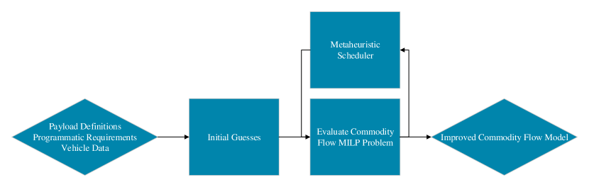
Figure 1: Overall structure of the generic campaign optimization problem [16].

2.1.1 Vehicle Data

The vehicle data input database file contains a list of logistics vehicles that are available for the lunar exploration campaign. Table 2 lists the parameters associated with each vehicle. The "secondary" parameters are determined based on the values of $I_{sp}$, which is used as a proxy for propellant type. $I_{sp}<370$ was taken to be a storable propellant type, $I_{sp}\geq 370$ s was taken to be cryogenic propellant. No high-$I_{sp}$ propulsion options such as electric or nuclear propulsion were considered. Throughout all case studies, oxidizer the boil-off rate was 0.016 fractional loss per day for liquid oxygen and 0 for storable propellants. Fuel boil-off was neglected. Table 3 gives an example of vehicle data input format, in which Vehicle 1 is a small lander and Vehicle 2 is a larger service module.

In addition to the list of vehicles, a list of vehicle “stacks” is defined. A “stack” is an aggregation of individual space vehicles into a single unit, that can be assembled through rendezvous or disconnected. The vehicle stacking system implemented in the linear program was inspired by the ontologies developed by Trent, Edwards et al, and Downs [17, 18, 19]. A vehicle stack is formatted as a list of its constituent vehicles and creates a new vehicle with the $I_{sp}$ and domain of the leading element, which is taken to be the active element. For example, referring to the example vehicles in Table 3, if the stack [2,1] is allowed, then Vehicle 3 becomes the stack and has the domain and $I_{sp}$ of Vehicle 2. Dry masses are summed together. The payload capability of the stack is the payload capability of the leading element minus the dry masses of the inactive elements.

Table 2: Definitions of the input vehicle parameters.

Parameter	Description
$m_{\mathrm{pay}}$	Payload capacity
$m_{\mathrm{prop}}$	Propellant capacity
$m_{\mathrm{dry}}$	Dry Mass
$I_{\mathrm{sp}}$	Specific impulse
$t_{F}$	Launch frequency
$t_{L}$	Earliest allowed launch
$\mathcal{D}$	Domain: a set of arcs along which the vehicle is allowed to travel.
Secondary Parameter	Description
$\phi$	Propellant oxidizer mass ratio
$\beta$	Boil-off rate

Table 3: Example vehicle data input.

Name	$m_{\mathrm{pay}}$, kg	$m_{\mathrm{prop}}$, kg	$m_{\mathrm{dry}}$, kg	$I_{\mathrm{sp}}$, s	$t_{F}$	$t_{L}$	$\mathcal{D}$
Vehicle 1	90	720	470	340	12	1	[0,0], [0,1], [1,2], [2,2], [2,3], [3,3]
Vehicle 2	1400	3320	1950	340	12	24	[0,0], [0,1], [1,2], [2,2]

2.1.2 Programmatic Requirements

The campaign program definition database file contains a list of payloads to be launched throughout the campaign. Table 4 lists the parameters associated with each payload. Payloads are indexed by $l\in[0,N_{p})$, where $N_{p}$ is the total number of campaign payloads. So, the first payload is $l=0$, for example. The sets of pre- and co-payloads contain the indices of those payloads. The type indices are the same as those used in [9, 16]. Table 5 gives an example of the payload data input format.

Table 4: Definitions of the programmatic parameters.

Parameter	Description
$p_{l}$	Payload type
$m_{l}$	Quantity/mass
$i_{l}$	Start node
$j_{l}$	Target node
$t_{L,l}$	Lower bound of launch window
$t_{U,l}$	Upper bound of launch window
$\mathcal{P}_{l}$	Set of soft precursors (payload $l$ must arrive before or with payloads in this set)
$\mathcal{Q}_{l}$	Set of strict precursors (payload $l$ must arrive strictly before payloads in this set)
$\mathcal{C}_{l}$	Set of co-payloads (payload $l$ must launch with payloads in this set)

Table 5: Example payload data input.

$\#$	Name	Type Index	Quantity	Supply Node $i$	Demand Node $j$	$t_{L}$	$t_{U}$	Co-Payloads
0	Crew	1	2	0	3	0	12
1	Science Payload	5	14	0	3	0	6	0

2.2 Metaheuristics Layer

The “outer layer” of the optimization algorithm searches for optimal launch schedules. A genetic algorithm is used, where the decision vector $\textbf{x}\in\boldsymbol{Z}^{N_{P}}$ contains the launch time of each payload in the campaign. The integer time steps chosen by the metaheuristics are a month in length. This allows for simplified synergy with the periodic nature of the low-energy transfers. x has the form $\textbf{x}=[t_{0},t_{1},...t_{N_{p}}]$

The genetic algorithm searches for solutions to the problem stated in Equation (1), where $\mathcal{F}$ is the output of the MILP, described in Section 2.3, given the input schedule x and set of programmatic requirements $\mathcal{R}$.

$$\begin{split}\min_{t_{l}}&\quad\mathcal{F}(\textbf{x}(t_{l}),\mathcal{R})\\ \text{s.t.}&\quad t_{L,l}\leq t_{l}\leq t_{U,l}\\ \end{split}$$ (1)

The metaheuristics problem is subject to constraints imposed by the programmatic payload-sequencing requirements. Equation (2) lists constraints corresponding to the soft precursor, strict precursor, and co-payload requirements respectively.

$$\begin{split}t_{q}-t_{l}\leq 0&\quad\forall\;q\in\mathcal{P}_{l}\\ t_{q}-t_{l}<0&\quad\forall\;q\in\mathcal{Q}_{l}\\ t_{q}-t_{l}=0&\quad\forall\;q\in\mathcal{C}_{l}\\ \end{split}$$ (2)

The metaheuristic-layer optimization was carried out using the genetic algorithm of the pygmo [20] metaheuristic optimization python library.

2.3 Logistics Mixed-Integer Linear Program (MILP) Layer

In space logistics, the transfer of vehicles, crew, payloads, and propellant are modeled as commodities flowing through a network. A mixed-integer linear program, an extension of the models described in [9, 16], is used to find the flow that results in a minimized launch mass, subject to certain constraints. Table 6 lists the constants, indices, and variables used in the linear program. Table 7 lists the locations represented in the model, and Table 8 lists the types of commodities and their costs. The cost of each commodity is its mass per unit.

Table 6: Definitions of the constants, indices, and variables used in the linear program.

Constant	Description
$N$	Total number of vehicles designs
$I$	Total number of network nodes
$P_{I}$	Number of integer commodity types
$P_{F}$	Number of float commodity types
$P=P_{I}+P_{F}$	Total number of commodity types
$T_{LP}$	Total number of time steps in the linear program
Index	Description
$n\in[0,N)$	Vehicle
$i\in[0,I)$	Start node
$j\in[0,I)$	Final node
$p\in[0,P)$	Payload type
$io\in\{0,1\}$	In-to- or out-of-arc
$t\in[0,T_{LP})$	Time
Variables	Description
$x_{n,i,j,p,io,t}$	Quantity of commodity type $p$, carried by vehicle $n$,
	from node $i$ to node $j$ at time $t$.
Terms	Description
$C_{n,j,p}$	Cost of launching commodity type $p$, carried by vehicle $n$,
	to node $j$ at time $t$.
$d_{n,i,p,t}$	Demand matrix defining the supply (positive value) or demand
	(negative value) of commodity type $p$, at node $i$ at time $t$.
$Z_{n,i,j}$	Propellant mass fraction associated with vehicle $n$
	travelling from node $i$ to node $j$.
$c$	Crew consumables consumption rate
$\rho$	ISRU propellant production rate
$\mu$	ISRU maintenance supply requirement
$\tau_{i,j,t}$	Real time of flight between node $i$ and node $j$ at discrete time index $t$
$\mathcal{E}_{i,j}$	Boolean variable defining whether the arc from node $i$ to node $j$ exists.

Table 7: Network nodes and arcs.

Node Index	Name	Arcs to
0	Earth Surface	0, 1
1	Low Earth Orbit (LEO)	0, 2
2	Low Lunar Orbit (LLO)	0, 1, 2, 3
3	Lunar Surface	2, 3

Table 8: Payload types and their costs per unit used in the logistics formulation. Payloads 0 and 1 are integer quantities, and payloads 2 - 7 are continuous quantities.

Index	Payload Type	Cost, kg per unit
0	Vehicle	$m_{dry}$
1	Crew	100
2	ISRU Plant	1
3	Maintenance Supplies	1
4	Crew Consumables	1
5	Miscellaneous Non-Consumable Payload	1
6	Oxidiser	1
7	Fuel	1

The network describes the Earth, Moon, and various orbits as “nodes”, and the transfers between them as “arcs”. Each arc has a cost ($\Delta V$) and a time-of-flight $\mathrm{TOF}$ associated with it. In a static network, only the nodes and the arcs representing their spacial separation are considered. The static network including the arc costs is shown in Figure 2. A network becomes “time-expanded” by repeating the static network across many discrete time steps, with “holdover” arcs connecting a location to its future counterpart. This is illustrated in Figure 3. The time expansion repeats with every second time step. That is to say, $\tau_{i,j,0}=\tau_{i,j,2}$. On these even time steps, only outbound flow is allowed. On odd time steps, return flow is allowed. A holdover arc on node 3 (lunar surface) from an even step to an odd step represents a short mission to the lunar surface, reminiscent of Apollo. The corresponding time of flight is 3 days. Meanwhile, the holdover arc in node 2 (lunar orbit) must equal the total of the time of flights for descent, surface stay, and ascent to maintain consistency, so its time of flight is 5 days. It is assumed that a long-duration mission would last some integer number of months, so the odd-to-even holdover arcs have time of flight such that 30 days have passed in total when returning to an even step. Node 0 (Earth surface) has a holdover arc, but no associated time of flight, because time of flight is only used in consumable loss calculations and this is not considered to be relevant pre-launch.

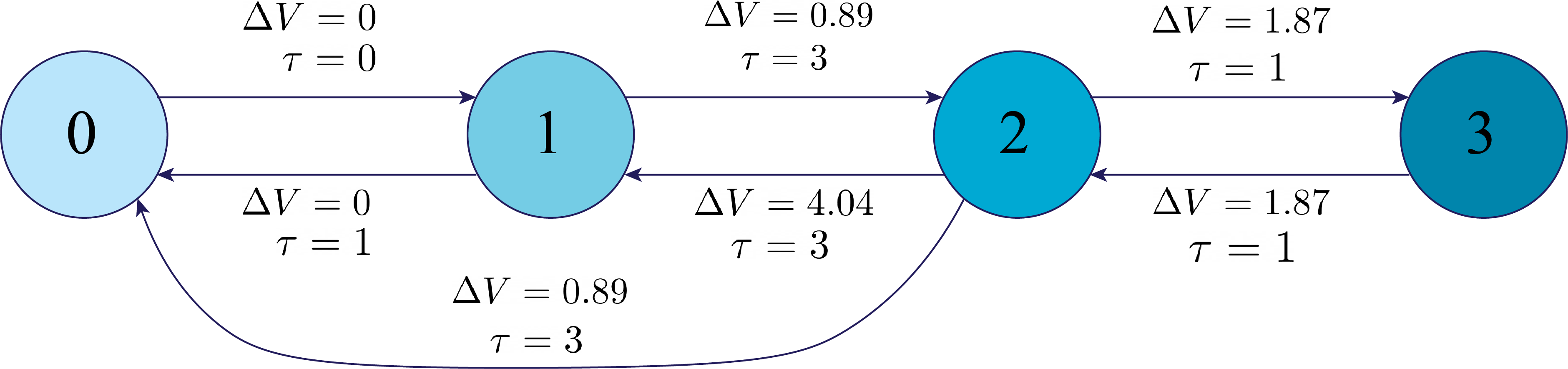
Figure 2: Diagram of the network model. $\Delta V$ measured in km s^-1, values from [21]. Lunar ascent neglects gravity losses. The arcs to and from the Earth node have 0 $\Delta V$ because it is assumed that a separate vehicle (launcher or reentry vehicle) from the logistics vehicle would make these transfers. Additionally, the $\Delta V$ from node 1 to node 2 is smaller than the reverse because it is assumed that the launch vehicle performs the lunar transfer injection. Time of flight measured in days. Adapted from [16].

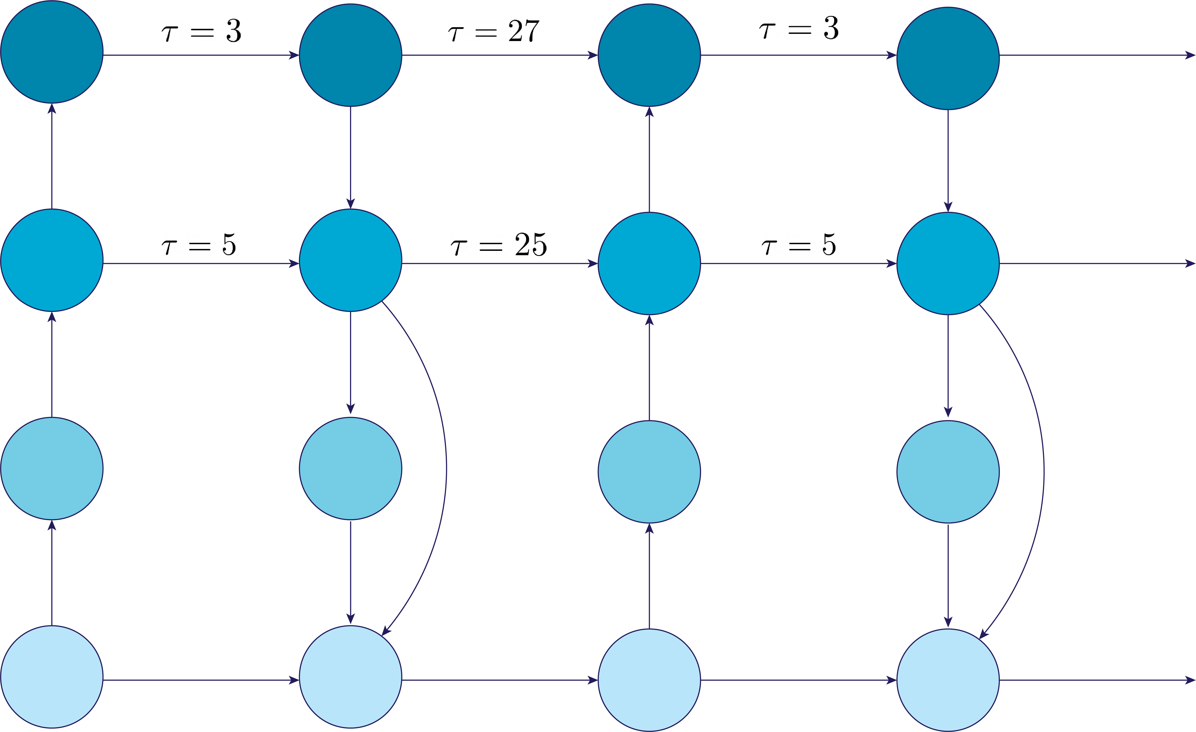
Figure 3: Diagram of the time-expanded network demonstrating the direction of commodity flow on each time step, including "time of flight" $t_{of}$ of the holdover arcs. Time of flight measured in days.

The objective of the MILP is to minimize the total mass delivered to LEO across the campaign, as specified in Equation (3).

$$\min_{x}f(x)=\sum_{t}\sum_{n}\sum_{p}\sum_{j}C_{p,n,j}x_{n,0,1,p,0,t}$$ (3)

Programmatic requirements are imposed on the commodity flow using a demand matrix $d_{n,i,p,t}$. This defines the supply or demand of commodities at specific nodes to be delivered at a specific time. Equations (4) and (5) state that the difference between the total amount of commodity flowing into a node from all others and the amount of the same commodity leaving the node to all others, is limited by the supply (positive value) or demand (negative value). Note that vehicles satisfy the demand/supply of their specific type, or vehicle stacks in which they appear, $\mathcal{S}_{n}$, whilst for all other payloads, only the sum of the payloads delivered by all logistics vehicles is considered. This allows commodities to transfer between vehicles, but maintain proper supply rules for the vehicles themselves.

$$c_{1a}(x):\quad\sum_{n\in\mathcal{S}_{n}}\sum_{j}\left(x_{n,i,j,p,0,t}-x_{n,j,i,p,1,t}\right)\leq d_{n,i,p,t}\quad\forall\;\mathcal{S},t\quad\text{if}\;p=0$$ (4)

$$c_{1b}(x):\quad\sum_{n}\sum_{j}\left(x_{n,i,j,p,0,t}-x_{n,j,i,p,1,t}\right)\sum_{n}\leq d_{n,i,p,t}\quad\forall\;t\quad\text{if}\;p>0$$ (5)

The second constraint enforces vehicle payload capacities. Crew, which are treated as integer payloads, have a mass of 100 kg per crew member. Note that the mass of the ISRU plants (index $p=2$) is excluded from the capacity for holdover arcs and the lunar surface as, in ISRU-based scenarios, they are intended to remain in place on the lunar surface independent of the movement of logistics vehicles.

$$c_{2}(x):\quad\begin{cases}100x_{n,i,j,1,0,t}+\sum_{p=2}^{5}x_{n,i,j,p,0,t}\leq x_{n,i,j,0,0,t}m_{pay,n},&\forall\;n,t\quad\text{if}\;i\neq j\;\text{or}\;i\neq 3\\[10.00002pt] 100x_{n,i,j,1,0,t}+\sum_{p=3}^{5}x_{n,i,j,0,0,t}\leq x_{n,i,j,0,0,t}m_{pay,n},&\forall\;n,t\quad\text{otherwise}\\ \end{cases}$$ (6)

The third constraint imposes the propellant capacity constraints.

$$c_{3a}(x):\quad x_{n,i,j,6,0,t}\leq x_{n,i,j,0,0,t}\>\phi_{n}\>m_{prop,n}\quad\forall\;n,t,i,j$$ (7)

$$c_{3b}(x):\quad x_{n,i,j,7,0,t}\leq x_{n,i,j,0,0,t}\>(1-\phi_{n})\>m_{prop,n}\quad\forall\;n,t,i,j$$ (8)

The fourth constraint ensures that changes in commodity quantities follow proper dynamics or conservation rules. Firstly, Equation (9) shows how crew consumables are consumed at a constant rate. In all case studies, a consumable rate of 8.655 kg per crew member per day was used, in consistency with [9].

$$c_{4a}(x):\quad x_{n,i,j,4,1,t}-x_{n,i,j,4,0,t}+c\>\tau_{i,j,t}\>x_{n,i,j,0,1,t}=0\quad\forall\;n,t,i,j$$ (9)

Equation (10) governs the maintenance supplies associated with ISRU infrastructure. The amount of maintenance supplies per day required is proportional to the mass of ISRU infrastructure present on the lunar surface.

$$c_{4b}(x):\quad\sum_{n}x_{n,3,3,3,1,t}-\sum_{n}x_{n,3,3,3,0,t}+\mu\>\tau_{3,3,t}\>x_{n,3,3,2,1,t}=0\quad\forall\;t$$ (10)

Equations (11) and (12) describe oxidizer and fuel consumption when traveling over arcs. Holdover arcs (except the lunar surface) suffer from oxygen boil-off, which is modeled as a fractional loss-per-day $\beta$. Holdover arcs on the lunar surface ($i=3$) allow for refueling from ISRU-produced propellant, produced at a constant rate $\rho$. Transfer arcs are sufficiently short that boil-off was neglected.

$$c_{4c}(x):\begin{cases}(1-\beta_{n})^{\tau_{i,j,t}}x_{n,i,j,6,1,t}-x_{n,i,j,6,0,t}=0&\forall\;n,t\quad\text{if}\;i=j\neq 3\\[10.00002pt] x_{n,i,j,6,1,t}-x_{n,i,j,6,0,t}+\rho\>\tau_{i,j,t}\sum_{n}x_{n,i,j,2,1,t}=0&\forall\;n,t\quad\text{if}\;i=j=3\\[10.00002pt] \phi_{n}Z_{n,i,j}\left(x_{n,i,j,0,0,t}m_{dry,n}+100x_{n,i,j,1,0,t}+\sum_{p=2}^{7}x_{n,i,j,p,1,t}\right)=0&\forall\;n,t,i,j\quad\text{otherwise}\\[10.00002pt] \end{cases}$$ (11)

$$\begin{split}c_{4d}(x):\quad&x_{n,i,j,7,1,t}-x_{n,i,j,7,0,t}+\\ &(1-\phi_{n})Z_{n,i,j}\left(x_{n,i,j,0,0,t}m_{dry,n}+100x_{n,i,j,1,0,t}+\sum_{p=2}^{7}x_{n,i,j,p,1,t}\right)=0\quad\forall\;n,t,i,j\end{split}$$ (12)

Equation (13) states that other commodities are simply conserved across arcs.

$$c_{4d}(x):\quad x_{n,i,j,p,1,t}-x_{n,i,j,p,0,t}=0\quad\forall\;n,t,i,j\quad\forall\;p\in\{0,1,3,4,5\}$$ (13)

The final constraint ensures that commodities only flow along arcs that exist at the current time step, and that vehicles remain within their domains.

$$c_{5}(x):\quad x_{n,i,j,p,io,t}=\begin{cases}0\quad\forall\;i,j,p,io\quad\text{if}\;[i,j]\notin\mathcal{D}_{n}\\[10.00002pt] 0\quad\forall\;n,p,io,t\quad\text{if}\;\mathcal{E}_{i,j}=0\\[10.00002pt] 0\quad\forall\;n,p,io\quad\text{if}\;i>j\;\text{and}\;t\;\text{even}\\[10.00002pt] 0\quad\forall\;n,p,io\quad\text{if}\;i<j\;\text{and}\;t\;\text{odd}\\[10.00002pt] \text{unconstrained otherwise}\end{cases}$$ (14)

To summarize, the MILP problem solved is shown in Equation (15).

$$\begin{split}\min_{x}&\quad\mathrm{Eqn.\;(\ref{eqn:LP_obj})}\\ \mathrm{s.t.}&\quad\mathrm{Eqns\;(\ref{eqn:LP_demand_constr_veh})\sim(\ref{eq:other_pay_constr})}\\ \end{split}$$ (15)

The MILP-layer commodity flow optimization was carried out using the Gurobi optimization software [22].

2.4 Model Construction

Two aspects of the commodity flow model change between iterations: the timeline, and the demand matrix. Both of these are determined by the decision vector chosen by the metaheuristic layer. Firstly, the metaheuristic chooses time stamps for each payload relative to the campaign timeline. So, for example, in a 12-month campaign, if payload 0 launches in the third month, then $t_{0}=2$ (indexing starts at 0). The MILP, however, only cares about time steps where events happen. So if another payload 1 launches in month 7, $t_{1}=6$, then the MILP does not consider what happens on months 0, 1, 3, 4, or 5. So, the 12-month campaign timeline is mapped onto a reduced timeline, which in this case only has 4 time steps (the 2 steps where launches occur, and the half-steps allowing for return flows). Of course, the “real” (non-reduced) time that has passed must be tracked between the reduced steps, so that consumable calculations are made properly. So for every time step that was cut from the campaign timeline when producing the reduced timeline, 30 days is added to the “time of flight” of the corresponding holdover arcs.

The demand matrix is generated by creating positive demands (supplies) at the source nodes specified in the programmatic input data, and negative demands at the targets nodes, of the quantity and type of payload specified, at the time indicated in the metaheuristic decision vector. Vehicles are also supplied according the to vehicle data file. One unit of a vehicle is supplied at Earth on its first available timestep, and subsequent units are supplied with every multiple of that vehicles launch frequency. If a timestep in the reduced timeline corresponds to multiple launch frequency periods of that vehicle, then the model construction algorithm calculates how many units should be added at the next step. The MILP commodity flow model was constructed using the Pyomo python library [23, 24].

2.5 Initial Feasible Guess Generation

The feasible space of the problem solved by the metaheuristic layer is very sparse, so it was necessary to create an algorithm that can generate pseudo-random (although naïve) initial feasible guesses, otherwise the feasible space is difficult to find. The guess generation method is summarised in Algorithm 1.

x = 0

  // Initialize x with 0’s.

v = rand (0, $Nv$)

  // Initialize a list of vehicles assigned to each payload with random choices.

1 for $i\in[0,N_{P}]$ do

2       if $\mathcal{C}_{i}\neq\emptyset$ then

3             $\textbf{x}[i]=\textbf{x}[j]\;,\;j\in\mathcal{C}_{i}$

4      

      $t_{L,i}=\max{\left(t_{L,i},\textbf{x}[j]\;\forall j\in\mathcal{P}_{i},\textbf{x}[j]+1\;\forall j\in\mathcal{Q}_{i}\right)}$

        // Update lower bound $t_{L,i}$ of $\textbf{x}[i]$ to whichever is most constraining between its programmatic lower bound, or launch times of any necessary pre-cursors.

5       if $t_{L,i}=t_{U,i}$ then

             x[i] = $t_{L,i}=t_{U,i}$

              // Only one feasible choice of launch time.

6            

       x[i] = rand($t_{L,i},t_{U,i}$)

        // If multiple choices are feasible, pick a random one.

      

       // Next, it is necessary to check that there are usable vehicles available at this time stamp.

7       while Valid Vehicle Check is False do

            

             // Maintain a list of vehicles which are valid for this payload. Initialize with full list of vehicles:

8             Valid Vehicle List = $[0,N]$

9             if Payload origin node is Earth then

10                   for $n\in[0,N]$ do

11                         if $t_{L,n}>\textbf{x}[i]$ then // Check vehicle $n$ is available at launch time x[i].

12                               Remove vehicle $n$ from the Valid Vehicle List.

13                        

14                  if Valid Vehicle List $\neq\emptyset$ then // If any valid vehicles remain, continue.

15                         for $n\in$ Valid Vehicle List do

                               Payload Mass = $m_{i}C_{i}$

                                // Check that the payload capacity of each vehicle is not broken by adding this payload.

16                              

17                              for $j\in[0,i]$ do // Find other payloads launching at the same time, on vehicle $n$.

18                                     if $\textbf{x}[i]=\textbf{x}[j]$ and $\textbf{v}[j]=n$ then

19                                           Payload Mass += $m_{j}C_{j}$

20                                    

21                              if Payload Mass $>m_{pay,n}$ then // If the payload capacity of vehicle $n$ is broken.

22                                     Remove vehicle $n$ from the Valid Vehicle List.

23                              

24                        

25                   if Valid Vehicle List $\neq\emptyset$ then // If any valid vehicles remain, continue.

26                         for $n\in$ Valid Vehicle List do // Check that the same vehicle is not used within a launch frequency period $t_{F,n}$

27                               for $j\in[0,i]$ do

28                                     if $\textbf{v}[j]=n$ and $0<\lvert\textbf{x}[j]-\textbf{x}[i]\rvert<t_{F,n}$ then

29                                           Remove vehicle $n$ from the Valid Vehicle List.

30                                    

31                              

32                        

33                  

34             for $n\in[0,N]$ do

35                   if $[3,2]\notin\mathcal{D}_{n}$ or $[2,0]\notin\mathcal{D}_{n}$ then // If payload not sourced at Earth, must be assigned to a return vehicle.

36                         Remove vehicle $n$ from the Valid Vehicle List.

37                  

38             if Valid Vehicle List $\neq\emptyset$ then

39                   $\textbf{v}[i]=$ rand(Valid Vehicle List)

                   Valid Vehicle Check = True

                    // Successfully found a valid vehicle for payload $i$.

40                  

             $t_{L,i}=$ rand($t_{L,i},t_{U,i}$)

              // If there are no valid vehicles, try a later time step.

41             if $t_{L,i}\neq t_{U,i}$ then

42                   x[i] = rand($t_{L,i},t_{U,i}$)

43             x[i] = $t_{L,i}$

44      

Algorithm 1 Initial feasible guess generator pseudo-code.

The objective of the algorithm is to find a launch time stamp for each payload in the programmatic requirements. It starts by checking the co-payload requirements, which if present would enforce a particular time stamp. If no co-payloads are found, then it checks for precursors. The allowed launch window is then updated with the new lower bound defined by the launch time of the most-constraining precursor. Then a random time stamp is chosen from the updated launch window. Finally, the algorithm checks that a suitable vehicle is available at this time stamp. If not, the launch window lower bound is set to the previous guess, and a new random-but-later time stamp is selected.

3 Results

This section will provide verification of both the commodity flow MILP and the metaheuristic scheduling algorithm. Then, the results of the Artemis program case studies will be presented and discussed.

3.1 Logistics MILP Verification Case: Apollo

Before moving on to the case studies, the commodity flow MILP is first verified using a simple, single-mission Apollo study. In this simplified Apollo model, 3 astronauts are launch from Earth, with two headed for the lunar surface, and one remaining in lunar orbit. 10 kg of payload (representing a rock sample) are carried on the return leg. This programmatic data is summarized in Table 9, and the available vehicles are summarized in Table 10. The allowed vehicle stacks are [2, 0, 1] and [0, 1]. The linear program is provided with the input decision vector $\textbf{x}(t_{l})=[0,0,0,0,0]$, indicating that the mission is launched and returned within the same time step (month), corresponding to a 3 day lunar surface mission.

The output of the linear program is summarized in Figure 4. The returned objective value (total mass to LEO) is 37486 kg. This is not dissimilar to the values found by logistics MILP developed by Chen et al [9], with discrepancies being attributed to updates to the model and deviations in input. However, it is short of the 43572 kg mass at lunar orbit injection burn start of Apollo 11 quoted by [25], due to the full inventory of payload and equipment not being included in this test.

Table 9: Apollo payload data input.

$\#$	Name	Type Index	Quantity	$i$	$j$	$t_{L}$	$t_{U}$	Co-Payloads
0	Lunar Surface Crew	1	2	2	3	0	0	1
1	Lunar Orbit Crew	1	3	0	3	0	0
2	Surface Crew Return	1	2	3	2	0	1	3
3	Orbit Crew Return	1	3	2	0	0	1
4	Sample Return	5	10	3	0	0	1	2

Table 10: Apollo vehicle data input. Lunar module (L.M.) data from [26], command module data from [25].

$\#$	Name	$m_{pay}$, kg	$m_{prop}$, kg	$m_{dry}$, kg	$I_{sp}$, s	$t_{F}$	$t_{L}$	$\mathcal{D}$
0	L.M. Descent Element	5300	8900	2217	311	1	0	[0,1], [2, 2], [2, 3], [3, 3]
1	L.M. Ascent Element	350	2670	2020	311	1	0	[0,1], [3, 3], [3, 2]
2	Command Module	22510	16870	11930	314.5	1	0	[0,1], [1,1], [1, 2], [2, 2],
								[2,0], [2,1], [1,0]

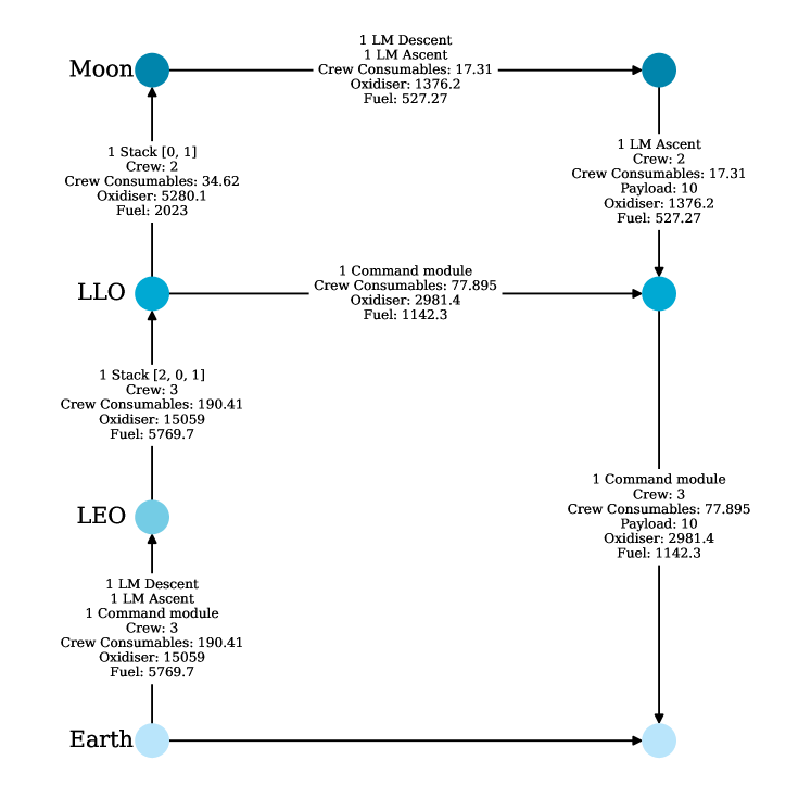
Figure 4: Optimal commodity flow calculated by the MILP given the Apollo programmatic inputs.

3.2 Metaheuristic Scheduler Verification Case: Commercial Lunar Payloads Services (CLPS) Program

Next, the campaign scheduling aspect of the method is demonstrated by applying it to the NASA CLPS program. The CLPS program is a planned series of payloads to be delivered to the lunar surface by private companies. The payloads are a series of scientific missions that are in support of the following Artemis program. It should be noted, that the primary aim of program is to fund the development of a wide variety of commercial lunar landers for future robustness of lunar exploration campaigns, and is not optimized for the most efficient delivery of the payloads. This means, though, that it provides a relatively easy case study in which to attempt to optimize the schedule of the campaign.

In the following ConOps definitions, time $t=0$ corresponds to the month of December 2022. The list of CLPS payloads considered in this analysis are listed in Table 11, and the vehicles are listed in Table 12. Stacking is not allowed in this ConOps. Note that this is not an exhaustive list of CLPS vehicles, but those with sufficient publicly available data to build the model are included. Results will be compared to an assumed baseline scenario which is illustrated in Figure 5.

Table 11: Payload data used in the CLPS analysis. Data quoted from sources where possible, and best approximations made otherwise. Time indices correspond to months with $t=0$ being December 2022. From [16]. Payload mass estimations were made according to publicly available information as of December 2022.

$\#$	Name	Type Index	Quantity	$i$	$j$	$t_{L}$	$t_{U}$	Co-Payloads $\mathcal{C}$
0	First shared payloads [27]	5	14	0	3	0	12
1	First shared payloads	5	14	0	3	0	12
2	CLPS-1 [27, 28]	5	50	0	3	0	12	0
3	Lunar Flashlight	5	12	0	2	0	12
4	CLPS-2 [27, 28]	5	50	0	3	0	12	1
5	CLPS-3 / PRIME-1 [29, 28]	5	36	0	3	7	12
6	CLPS-4 [28]	5	300	0	3	13	13
7	CLPS-5 [28]	5	50	0	3	13	24
8	VIPER [30, 28]	5	430	0	3	12	25
9	Mare Crisium mission [31, 28]	5	94	0	3	13	25
10	Schrödinger mission [32, 28]	5	95	0	3	25	36

Table 12: Lunar lander data used in the CLPS analysis. Data quoted from sources where possible, and best approximations made otherwise. For example, assumptions about launch mass have been made based on the assumed launch vehicle in some cases. Time indices correspond to months with $t=0$ being December 2022. Adapted from [16].

$\#$	Name	$m_{pay}$, kg	$m_{prop}$, kg	$m_{dry}$, kg	$I_{sp}$, s	$t_{F}$	$t_{L}$	$\mathcal{D}$
0	Astrobotic "Peregrine" [33]	90	720	470	340	12	1	[0,0], [0,1], [1, 2], [2,3], [3,3]
1	Astrobotic "Griffin" [34, 35]	630	3320	1950	340	12	24	[0,0], [0,1], [1, 2], [2,3], [3,3]
2	B.O. "Blue Moon" [36, 37]	4500	6350	2150	420	12	24	[0,0], [0,1], [1, 2], [2,3], [3,3]
3	ispace S1 [38]	30	700	300	340	12	0	[0,0], [0,1], [1, 2], [2,3], [3,3]
4	Draper/ispace S2 [39]	500	3380	2120	340	12	13	[0,0], [0,1], [1, 2], [2,3], [3,3]
5	Firefly "Blue Ghost" [40]	155	3380	2470	340	12	13	[0,0], [0,1], [1, 2], [2,3], [3,3]
6	I.M. "Nova-C" [41]	100	1010	790	370	6	0	[0,0], [0,1], [1, 2], [2,3], [3,3]
7	L.M. "McCandless" [42]	350	3380	2270	340	12	48	[0,0], [0,1], [1, 2], [2,3], [3,3]
8	M.E. MX-1 "Scout" [43]	30	150	70	320	12	48	[0,0], [0,1], [1, 2], [2,3], [3,3]

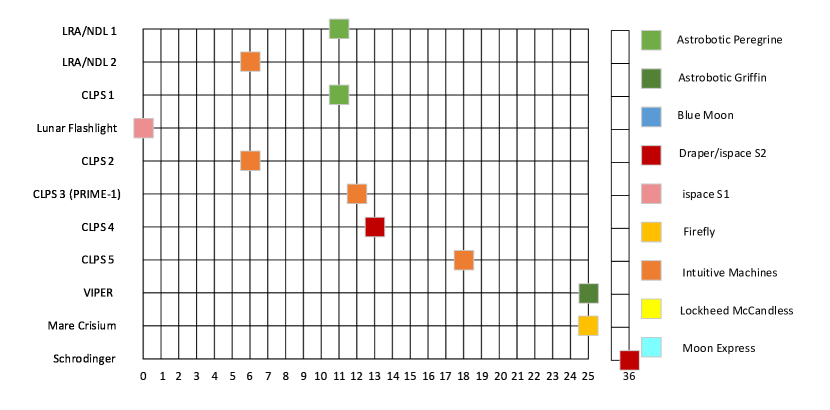
Figure 5: Assumed baseline schedule and vehicle assignments of the CLPS campaign. Adapted from [16], based on assumptions made from publicly available data as of December 2022. Updated with real-world delays as of May 2023.

The MILP level input decision vector that corresponds to the baseline scenario of Figure 5 is:

$$\textbf{x}=[11,6,11,0,6,12,13,18,25,25,36]$$

First, this vector is passed to the MILP which will solve the commodity flow optimization. The output commodity flow is shown in Figure 6, with an objective value of 19061 kg. Note that the vehicle assignments here do not match those assumed in the baseline scenario - this is because the vehicles themselves are treated as commodities, so payload-to-vehicle assignment is optimized at the MILP level.

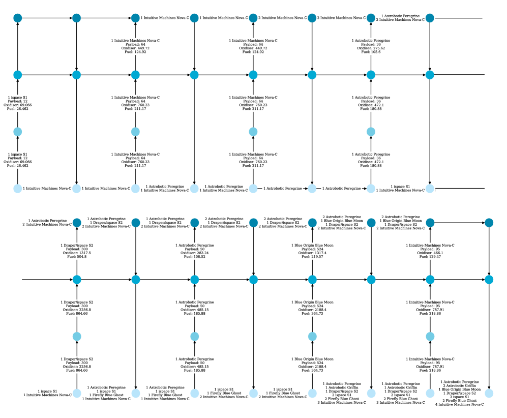
Figure 6: CLPS ConOps with baseline launch schedule and optimized commodity flown.

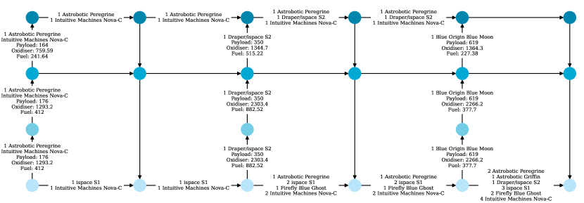
Figure 7: CLPS ConOps with both optimized schedule and optimized commodity flow.

Next, the overall campaign will be optimized using the metaheuristic schedule optimizer. This was done by generating 20 initial feasible guesses using Algorithm 1 and using them to initialize the genetic algorithm population. 5 such populations were initialized as pygmo “island” objects. Islands are a framework for parallelized function evaluation with metaheuristic optimization algorithms [44]. Then, the genetic algorithm evolved the “archipelago” of islands through 200 generations with a mutation probability of 0.05. With each generation, the best solutions can migrate between islands, providing a form of parallelized evolution. The best-found solution through this evolution returned an objective of 14207 kg, which was found after 29 generations / 590 MILP evaluations. The commodity flow for the optimized launch schedule is shown in Figure 7.

As stated in the introduction, commodity flow LPs can handle scheduling with constraints no more complex than upper and lower bounds. Therefore, the CLPS case study also serves as a verification case for the scheduling algorithm, as the scheduling requirements are simple enough that they can be handled directly by the logistics MILP algorithm if Payloads 0 and 1 from Table 11 are directly combined with payloads 2 and 4 such that the co-payloads requirements $\mathcal{C}$ were enforced. The new model was constructed by creating a new demand matrix in which the supply time is defined as the lower bound of the payload’s availability window $t_{L}$ and the demand time is defined as the upper bound of the availability window $t_{U}$. When this new model is solved, an objective of 14207 kg is found, verifying that the scheduling algorithm found an optimal schedule.

3.3 Case Study 1: Artemis Phases 1 and 2A

The first full case study expands the CLPS case to include the lunar surface missions of Artemis Phases 1 and 2A. Artemis Phase 1 is assumed to include the CLPS missions and the first crewed lunar landing (Artemis 3). Phase 2A then consists of the following surface missions up to Artemis 6. Artemis missions 3 - 5 are all 3 day missions (in terms of the timeline used in the metaheuristic scheduling algorithm, the return missions happens in the same time step as the outbound), whereas Artemis 6 is required to be at least a month long. Artemis 5 has the pressurized crew rover as a pre-requisite payload. The list of payloads in the campaign is appended with those listed in Table 13 and the list of available vehicles is appended with those in Table 14. The allowed vehicle stacks are [12, 10, 11], [10, 11], and [12, 11].

Again, an initial population of 20 random feasible guesses was generated using Algorithm 1, and used to populate 5 islands. The islands were evolved through 400 generations, again with cross-migrations. In this analysis, a smaller mutation probability of 0.01 was used. This is because the decision vector is larger, due to the larger list of payloads, so there are more opportunities for mutations to occur. The smaller probability was used to balance this so that the overall mutation rate did not increase.

The best found solution is shown in Figure 10 (from here onward, unused vehicles remaining at the Earth node will not be shown for simplicity). The solution shows a quirk of the commodity flow model in that, in December 2027, the crew are launched on CLPS vehicle and rendezvous with a pre-launched Orion capsule in lunar orbit. The commodity flow solver chose this solution because it is agnostic to whether a vehicle is a crew-rated or not, and the Blue Origin lander has the highest $I_{sp}$ of the available vehicles. Though this could easily be implemented in future models if necessary, it does of course indicate the value of high-$I_{sp}$ crewed vehicles.

Table 13: Additonal payload data used in the Artemis phase 1 and 2A analysis. Data quoted from sources where possible, and best approximations made otherwise. Time indices correspond to months with $t=0$ being December 2022. From [16]. Payload mass estimations were made according to publicly available information as of December 2022.

$\#$	Name	Type Index	Quantity	$i$	$j$	$t_{L}$	$t_{U}$	$\mathcal{P}$	$\mathcal{Q}$	$\mathcal{C}$
11	LUPEX [45]	5	350	0	3	25	36
12	LEAP Rover [46]	5	30	0	3	37	48
13	Unpressurised Crew Rover	5	300	0	3	12	24
14	Artemis 3 Launch	1	2	0	2	24	39
15	Artemis 3 Landing	1	2	2	3	24	39			14
16	Artemis 3 Ascent	1	2	3	2	24	39			14
17	Artemis 3 Return	1	2	2	0	24	39			14
18	Artemis 4 Launch	1	2	0	2	40	55
19	Artemis 4 Landing	1	2	2	3	40	55			18
20	Artemis 4 Ascent	1	2	3	2	40	55			18
21	Artemis 4 Return	1	2	2	0	40	55			18
22	ISRU demo	2	300	0	3	37	49
23	Small Pressurised Rover	5	4000	0	3	56	71
24	Artemis 5 Launch	1	2	0	2	56	71	23
25	Artemis 5 Landing	1	2	2	3	56	71			24
26	Artemis 5 Ascent	1	2	3	2	56	71			24
27	Artemis 5 Return	1	2	2	0	56	71			24
28	Artemis 6 Launch	1	4	0	2	72	87
29	Artemis 6 Landing	1	4	2	3	72	87			28
30	Artemis 6 Ascent	1	4	3	2	72	87		28
31	Artemis 6 Return	1	4	2	0	72	87			30

Table 14: Additonal lunar lander data used in the Artemis phase 1 and 2A analysis. Data quoted from sources where possible, and best approximations made otherwise. The figures regarding the Orion spacecraft differ from the real-world equivalent because this model requires that Orion deliver its crew to LLO, rather than the real-world requirement of higher lunar orbits such as NRHOs. Time indices correspond to months with $t=0$ being December 2022. Adapted from [16].

$\#$	Name	$m_{pay}$, kg	$m_{prop}$, kg	$m_{dry}$, kg	$I_{sp}$, s	$t_{F}$	$t_{L}$	$\mathcal{D}$
9	ESA EL3 [47]	1800	5580	2520	340	24	84	[0,1], [1, 2], [2,3], [3,3]
10	ISECG lander [48]	9000	23660	9340	340	12	12	[0,0], [0,1], [2,2], [2,3], [3,3]
11	ISECG ascender	500	10000	1000	340	12	12	[0,0], [0,1], [3,3], [3,2]
12	Orion	11800	22000	16520	316	12	0	[0,0], [0,1], [1,1], [1,2],
								[2,2], [2,0], [2,1], [1,0]
13	JAXA/ISRO lander [45]	350	3510	2140	320	36	25	[0,1], [1, 2], [2,3], [3,3]

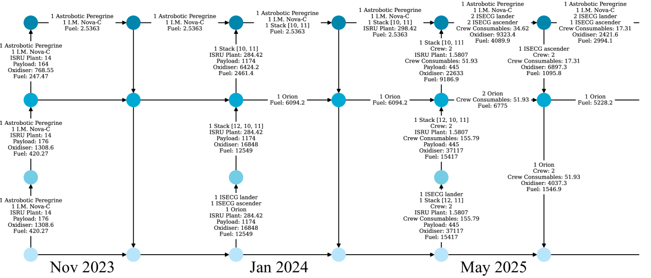
Figure 8: (continued on next page).

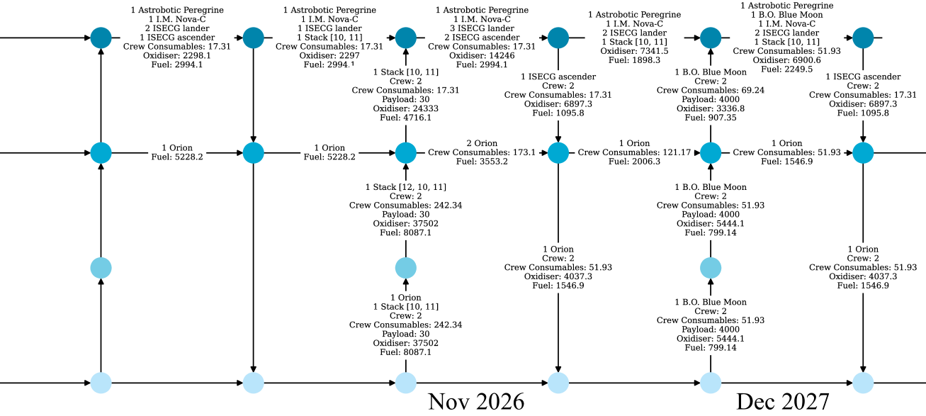
Figure 9: (continued on next page).

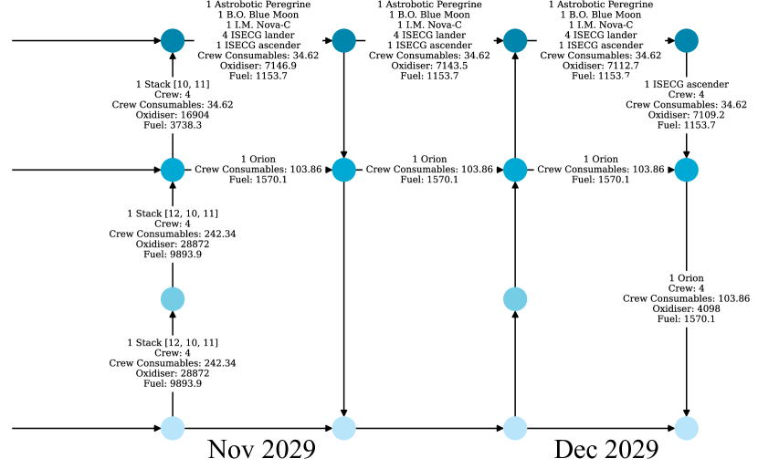
Figure 10: Artemis phase 1 and 2A ConOps with optimized schedule and optimized commodity flow.

Table 15: Number of times each vehicle was used in the optimized Artemis phase 1 and 2A ConOps.

Name	No. times used
Astrobotic Peregrine	1
I.M Nova-C	1
B.O. Blue Moon	1
ISECG lander	4
ISECG ascender	4
Orion	4

Table 15 summarizes the number of times that vehicles were used in the optimized Artemis phase 1 and 2A ConOps. It can be seen that the optimal solution features only a small number of the available vehicles, with the optimal strategy typically being to include as many payloads in the larger capacity crewed launches as the programmatic requirements allow. Although the unused vehicles do not contribute to the optimal results within the constraints of the ambiguous campaign definition, they would have usefulness in terms of robustness against certain aleatory uncertainties such as payload development delays.

3.4 Case Study 2: Artemis Phase 2B

A major advantage of the development of time-expanded commodity flow models for space logistics [7, 9] is the ability to model the impact that in-situ resource utilization (ISRU) infrastructure has on the overall logistics of a campaign. This final case study looks to demonstrate how this can improve longer-term campaign planning and scheduling, in addition to testing a more complex set of programmatic requirements with a much larger solution space. To do this, the case study will consider the Artemis Phase 2B scenario, building towards the sustainable permanent lunar outpost of Artemis Phase 3, or the "Moon Village" concepts [49]. It features the delivery of large habitation and power generation elements, and pressurized rovers. Phase 2B includes crewed missions 7 through 14, each with large sample return masses. Finally, because the impact of ISRU on the campaign was to be studied, "Mk 2" versions of the ISECG vehicles were added to the scenario, each assumed to have the same dry masses and propellant capacities but with upgraded $I_{sp}$ of 370s, indicating the upgrade to ISRU-compatible cryogenic propellant. The payload capabilities of the lander were expanded accordingly with the new $I_{sp}$.

In the following analysis, an ISRU infrastructure maintenance supply delivery rate of $10\%$ of the total infrastructure mass per year is used. The rate of production of in-situ produced oxygen was calculated using the parametric sizing model developed by Schreiner et al [50]. Figure 10 of [50] offers values for reactor mass and power requirements as a function of production rate. From this, a relatively conservative production rate value of $m_{R}=2000$ kg oxygen per year per kg of reactor mass is chosen, with a power requirement of $\alpha=10$ W per kg oxygen per year. The power requirement is then converted to a power system mass using data from the NASA Small Fission Power System study [51], in which Table 1 offers expected specific power (W per kg) for multi-kW capable, lunar surface fission reactors. A specific power of $\gamma=6.5$ W per kg is used here. With values for reactor mass, reactor power requirements, and power system mass, the total resource production rate per ISRU infrastructure mass can be calculated according to Equation (16. With the quoted values, the resulting ISRU oxygen production rate is 0.00153 kg oxygen per day per kg of infrastructure.

$$\rho=\left(\frac{1}{m_{R}}+\frac{\alpha}{\gamma}\right)^{-1}$$ (16)

The Artemis Phase 2B campaign is defined in this analysis by the list of payloads in Table 16. These payloads are adapted from [52]. $t=0$ is undefined, assumed to be some date later than the December 2029 end date of the Artemis 1 and 2A analysis. The same list of vehicles from the previous case studies is used again, with the lower bound of availability removed, as this campaign is further in the future. The additional Mk 2 ISECG vehicles are listed in Table 17. Additional vehicle stacks are defined such that the Mk2 landers can stack together, as well as mixed stacks of Mk1 and Mk2 landers.

Table 16: Payload data used in the Artemis phase 2B analysis. Adapted from [52].

$\#$	Name	Type Index	Quantity	$i$	$j$	$t_{L}$	$t_{U}$	$\mathcal{P}$	$\mathcal{Q}$	$\mathcal{C}$
0	Power Plant element	5	1500	0	3	0	48
1	Artemis 7 Crew	1	4	0	2	0	48	0
2	Artemis 7 Crew Landing	1	4	2	3	0	48			1
3	Artemis 7 Crew Ascent	1	4	3	2	0	48		2
4	Artemis 7 Crew Return	1	4	2	0	0	48			3
5	Sample return	5	200	3	0	0	48
6	Habitat	5	4500	0	3	0	54
7	Artemis 8 Crew	1	4	0	2	0	54	6	4
8	Artemis 8 Crew Landing	1	4	2	3	0	54			7
9	Artemis 8 Crew Ascent	1	4	3	2	0	54		8
10	Artemis 8 Crew Return	1	4	2	0	0	54			9
11	Sample return	5	200	3	0	0	54
12	Artemis 9 Crew	1	4	0	2	12	60		10
13	Artemis 9 Crew Landing	1	4	2	3	12	60			12
14	Artemis 9 Crew Ascent	1	4	3	2	12	60		13
15	Artemis 9 Crew Return	1	4	2	0	12	60			14
16	Sample return	5	200	3	0	12	60
17	Pressurised Rover	5	4500	0	3	0	66
18	Pressurised Rover	5	4500	0	3	0	66
19	Artemis 10 Crew	1	4	0	2	24	66	17, 18	15
20	Artemis 10 Crew Landing	1	4	2	3	24	66			19
21	Artemis 10 Crew Ascent	1	4	3	2	24	66		20
22	Artemis 10 Crew Return	1	4	2	0	24	66			21
23	Sample return	5	200	3	0	24	66
24	Artemis 11 Crew	1	4	0	2	36	72		22
25	Artemis 11 Crew Landing	1	4	2	3	36	72			24
26	Artemis 11 Crew Ascent	1	4	3	2	36	72		25
27	Artemis 11 Crew Return	1	4	2	0	36	72			26
28	Sample return	5	200	3	0	36	72
29	Artemis 12 Crew	1	4	0	2	48	84		27
30	Artemis 12 Crew Landing	1	4	2	3	48	84			29
31	Artemis 12 Crew Ascent	1	4	3	2	48	84		30
32	Artemis 12 Crew Return	1	4	2	0	48	84			31
33	Sample return	5	200	3	0	48	84
34	Fission Power Plant	5	4500	0	3	48	84
35	Habitat	5	4500	0	3	48	84
36	Artemis 13 Crew	1	4	0	2	60	96	34, 35	32
37	Artemis 13 Crew Landing	1	4	2	3	60	96			36
38	Artemis 13 Crew Ascent	1	4	3	2	60	96		37
39	Artemis 13 Crew Return	1	4	2	0	60	96			38
40	Sample return	5	200	3	0	60	96
41	Artemis 14 Crew	1	4	0	2	72	96		39
42	Artemis 14 Crew Landing	1	4	2	3	72	96			41
43	Artemis 14 Crew Ascent	1	4	3	2	72	96		42
43	Artemis 14 Crew Return	1	4	2	0	72	96			43
44	Sample return	5	200	3	0	72	96

Table 17: Mk 2 ISECG vehicles used in the Artemis 2B analysis.

$\#$	Name	$m_{pay}$, kg	$m_{prop}$, kg	$m_{dry}$, kg	$I_{sp}$, s	$t_{F}$	$t_{L}$	$\mathcal{D}$
14	MK2 ISECG lander	11390	23660	9340	370	12	0	[0, 0], [0,1], [2, 2], [2, 3], [3, 3]
15	MK2 ISECG ascender	500	10000	1000	370	12	0	[0, 0], [0, 1], [3, 3], [3, 2]

20 initial feasible guesses were generated using Algorithm 1. Theses guesses were used to initialize two metaheuristic algorithm populations. Only two population islands were used in this analysis because of the larger computing power requirements of the increased model size. A mutation probability of 0.01 was used.

After evolution through 40 generations, the objective value improved from 886750 kg to 819650 kg. The commodity flow produced by this solution is shown in Figure 17.

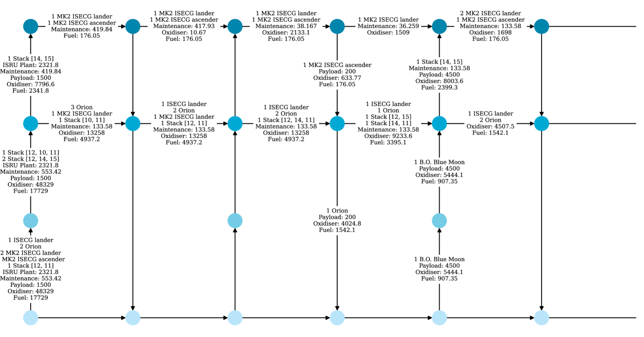
Figure 11: (continued on next page).

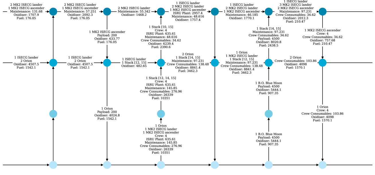
Figure 12: (continued on next page).

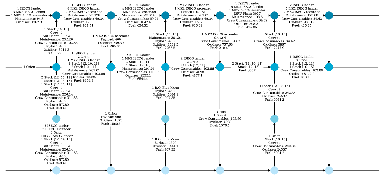
Figure 13: (continued on next page).

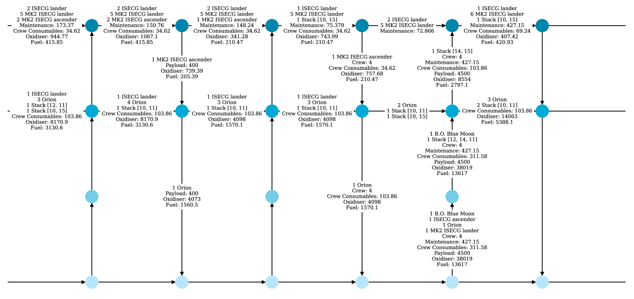
Figure 14: (continued on next page).

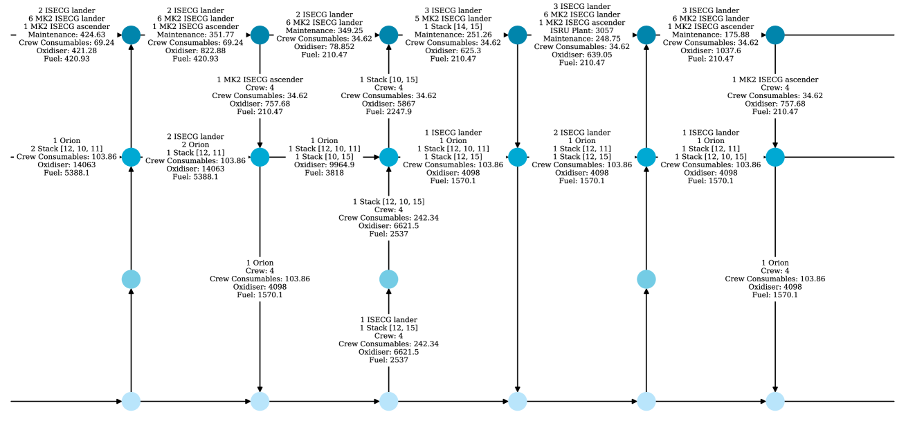
Figure 15: (continued on next page).

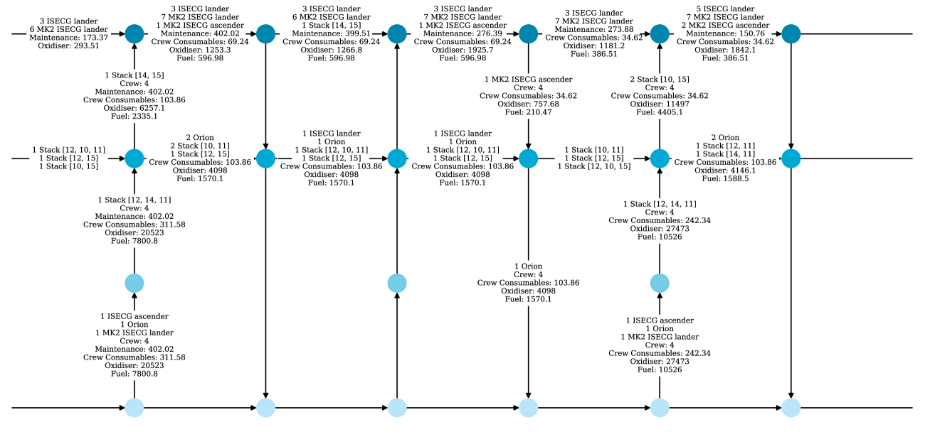
Figure 16: (continued on next page).

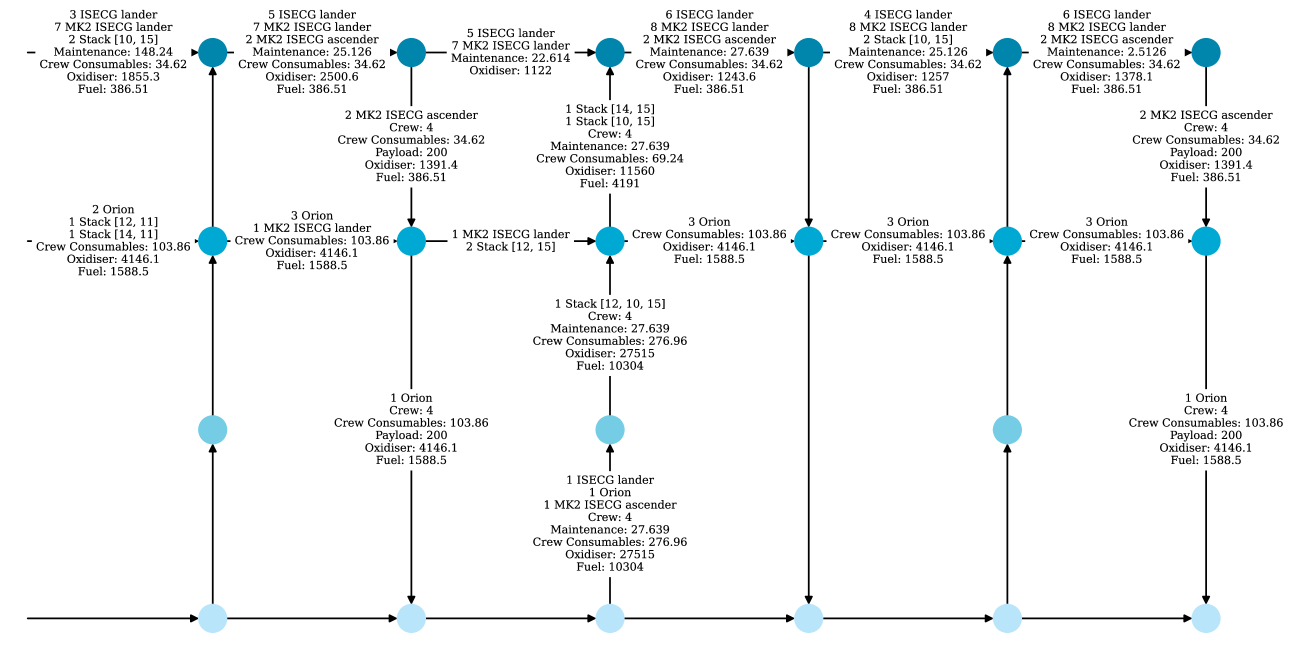
Figure 17: Artemis phase 2B ConOps with improved schedule and optimized commodity flow.

As expected, it can be seen that the commodity flow optimizer ships ISRU infrastructure and maintenance supplies with the first mission of the campaign. Further maintenance supplies are shipped with later missions. The inclusion of ISRU infrastructure prompts the scheduler to place the later missions later in their allowed windows, so that more propellant can be produced in-situ and reduce the amount required to be launched from Earth.

4 Conclusion

This paper has presented a method for finding feasible exploration campaign plans subject to programmatic requirements, and in particular finding schedules that produce optimal commodity flow such that total launch mass across the entire campaign is minimized. By using a mixed-integer linear program to solve the optimal commodity flow for a given campaign plan, a genetic algorithm can then be used to find improved schedules. The scheduling algorithm was verified against the output of the commodity flow LP without scheduling constraints. In a series of case studies, it was found that medium-to-large class lunar landers are most effective in optimizing lunar exploration logistics and, in cases of low availability of those landers, smaller and readily available landers provide useful, though sub-optimal, alternatives.

Acknolwedgment

The authors acknowledge Yuri Shimane and Masafumi Isaji for their helpful feedback and suggestions.

References

- International Space Exploration Coordination Group (2020) [ISECG] International Space Exploration Coordination Group (ISECG), Global Exploration Roadmap (GER) Supplement August 2020: Lunar Surface Exploration Scenario Update, 2020. URL https://www.globalspaceexploration.org/wp-content/uploads/2020/08/GER_2020_supplement.pdf.
- Fasano [1996] Fasano, G., “Mixed integer linear approach for the space station on-orbit resources re-supply,” AIRO 96 Annual Conference Proceedings, Perugia, Italy, 1996.
- Fasano and Provera [1997] Fasano, G., and Provera, R., “A traffic model for the space station on-orbit re-supply problem,” The International Society of Logistics Engineering (SOLE), Logistics National Conference Proceedings, Turin, Italy, 1997.
- Taylor et al. [2006] Taylor, C., Klabjanz, D., Simchi-levi, D., Song, M., and De Weck, O., “Modeling Interplanetary Logistics: A Mathematical Model for Mission Planning,” AIAA Journal, 2006. 10.2514/6.2006-5735.
- Gralla et al. [2006] Gralla, E., Shull, S., and de Weck, O., “A Modeling Framework for Interplanetary Supply Chains,” Space 2006, American Institute of Aeronautics and Astronautics, San Jose, California, 2006. 10.2514/6.2006-7229, URL http://arc.aiaa.org/doi/10.2514/6.2006-7229.
- Grogan et al. [2011] Grogan, P., Yue, H., and De Weck, O., “Space Logistics Modeling and Simulation Analysis using SpaceNet: Four Application Cases,” AIAA SPACE 2011 Conference Exposition, American Institute of Aeronautics and Astronautics, Long Beach, California, 2011. 10.2514/6.2011-7346.
- Ho et al. [2014] Ho, K., de Weck, O., Hoffman, J., and Shishko, R., “Dynamic modeling and optimization for space logistics using time-expanded networks,” Acta Astronautica, Vol. 105, 2014. 10.1016/j.actaastro.2014.10.026.
- Ishimatsu et al. [2016] Ishimatsu, T., de Weck, O. L., Hoffman, J. A., Ohkami, Y., and Shishko, R., “Generalized Multicommodity Network Flow Model for the Earth–Moon–Mars Logistics System,” Journal of Spacecraft and Rockets, Vol. 53, No. 1, 2016, p. 25–38. 10.2514/1.A33235.
- Chen and Ho [2018] Chen, H., and Ho, K., “Integrated Space Logistics Mission Planning and Spacecraft Design with Mixed-Integer Nonlinear Programming,” Journal of Spacecraft and Rockets, Vol. 55, No. 2, 2018, p. 365–381. 10.2514/1.A33905.
- Isaji et al. [2021] Isaji, M., Takubo, Y., and Ho, K., “Multidisciplinary Design Optimization Approach to Integrated Space Mission Planning and Spacecraft Design,” Journal of Spacecraft and Rockets, Vol. 59, No. 5, 2021, p. 1660–1670. 10.2514/1.A35284.
- Chen et al. [2021a] Chen, H., Sarton du Jonchay, T., Hou, L., and Ho, K., “Multifidelity Space Mission Planning and Infrastructure Design Framework for Space Resource Logistics,” Journal of Spacecraft and Rockets, Vol. 58, No. 2, 2021a, p. 538–551. 10.2514/1.A34666.
- Takubo et al. [2022] Takubo, Y., Chen, H., and Ho, K., “Hierarchical Reinforcement Learning Framework for Stochastic Spaceflight Campaign Design,” Journal of Spacecraft and Rockets, Vol. 59, No. 2, 2022, p. 421–433. 10.2514/1.A35122.
- Blossey [2023] Blossey, G., “A Stochastic Modeling Approach for Interplanetary Supply Chain Planning,” Space: Science & Technology, Vol. 3, 2023, p. 0014. 10.34133/space.0014.
- Chen et al. [2021b] Chen, H., Gardner, B. M., Grogan, P. T., and Ho, K., “Flexibility Management for Space Logistics via Decision Rules,” Journal of Spacecraft and Rockets, Vol. 58, No. 5, 2021b, p. 1314–1324. 10.2514/1.A34985.
- Sarton du Jonchay et al. [2021] Sarton du Jonchay, T., Chen, H., Gunasekara, O., and Ho, K., “Framework for modeling and optimization of on-orbit servicing operations under demand uncertainties,” Journal of Spacecraft and Rockets, Vol. 58, No. 4, 2021, pp. 1157–1173.
- Gollins et al. [2023] Gollins, N. J., Isaji, M., Shimane, Y., and Ho, K., “A Heuristic Method for Determining Payload-to-Vehicle Assignment Launch Order for Multi-Vehicle Exploration Campaigns,” AIAA SCITECH 2023 Forum, American Institute of Aeronautics and Astronautics, National Harbor, MD, 2023. 10.2514/6.2023-1965, URL https://arc.aiaa.org/doi/10.2514/6.2023-1965.
- Trent [2017] Trent, D., “Integrated Architecture Analysis and Technology Evaluation for Systems of Systems Modeled at the Subsystem Level,” Ph.D. thesis, Georgia Institute of Technology, Atlanta, GA, Nov 2017. URL https://repository.gatech.edu/entities/publication/79512a85-fe5f-4f18-9ef3-ffbb29df593e.
- Edwards et al. [2018] Edwards, S. J., Trent, D., Diaz, M. J., and Mavris, D. N., “A Model-Based Framework for Synthesis of Space Transportation Architectures,” 2018 AIAA SPACE and Astronautics Forum and Exposition, American Institute of Aeronautics and Astronautics, Orlando, FL, 2018. 10.2514/6.2018-5133, URL https://arc.aiaa.org/doi/10.2514/6.2018-5133.
- Downs et al. [2023] Downs, C., Prasad, A., Robertson, B. E., and Mavris, D. N., “A Spaceflight Logistics Approach to Modeling Novel Vehicle Concepts,” AIAA SCITECH 2023 Forum, American Institute of Aeronautics and Astronautics, National Harbor, MD Online, 2023. 10.2514/6.2023-1964, URL https://arc.aiaa.org/doi/10.2514/6.2023-1964.
- Biscani and Izzo [2020] Biscani, F., and Izzo, D., “A parallel global multiobjective framework for optimization: pagmo,” Journal of Open Source Software, Vol. 5, No. 53, 2020, p. 2338. 10.21105/joss.02338, URL https://doi.org/10.21105/joss.02338.
- Parker and Anderson [2014] Parker, J. S., and Anderson, R. L., Low-Energy Lunar Trajectory Design, John Wiley Sons, Inc., Hoboken, NJ, USA, 2014. 10.1002/9781118855065, URL http://doi.wiley.com/10.1002/9781118855065.
- Gurobi Optimization, LLC [2022] Gurobi Optimization, LLC, “Gurobi Optimizer Reference Manual,” , 2022. URL https://www.gurobi.com.
- Hart et al. [2011] Hart, W. E., Watson, J.-P., and Woodruff, D. L., “Pyomo: modeling and solving mathematical programs in Python,” Mathematical Programming Computation, Vol. 3, No. 3, 2011, pp. 219–260.
- Bynum et al. [2021] Bynum, M. L., Hackebeil, G. A., Hart, W. E., Laird, C. D., Nicholson, B. L., Siirola, J. D., Watson, J.-P., and Woodruff, D. L., Pyomo–optimization modeling in python, 3rd ed., Vol. 67, Springer Science & Business Media, 2021.
- Orloff [2000] Orloff, R. W., Apollo by the numbers: a statistical reference, NASA-SP, National Aeronautics and Space Administration, Washington, D.C, 2000.
- Isaji et al. [2020] Isaji, M., Maynard, I., and Chudoba, B., “A New Sizing Methodology for Lunar Surface Access Systems,” AIAA Scitech 2020 Forum, American Institute of Aeronautics and Astronautics, Orlando, FL, 2020. 10.2514/6.2020-1775, URL https://arc.aiaa.org/doi/10.2514/6.2020-1775.
- Warner [2020] Warner, C., “First Commercial Moon Delivery Assignments to Advance Artemis,” NASA, 2020. URL http://www.nasa.gov/feature/first-commercial-moon-delivery-assignments-to-advance-artemis, accessed: 2023-05-29.
- Dunbar [2019] Dunbar, B., “Commercial Lunar Payload Services Overview,” NASA, 2019. URL http://www.nasa.gov/content/commercial-lunar-payload-services-overview, accessed: 2022-11-18.
- Vitug [2020] Vitug, E., “Polar Resources Ice Mining Experiment-1 (PRIME-1),” NASA, 2020. URL http://www.nasa.gov/directorates/spacetech/game_changing_development/projects/PRIME-1, accessed: 2022-11-18.
- Colaprete [2020] Colaprete, A., “A lunar water reconnaissance mission,” NASA, 2020, p. 25. URL https://science.nasa.gov/science-pink/s3fs-public/atoms/files/09-Colaprete-VIPER%20Overview%20for%20PAC%2008172020.pdf, accessed: 2022-11-18.
- Potter [2021] Potter, S., “NASA Selects Firefly Aerospace for Artemis Commercial Moon Delivery,” NASA, 2021. URL http://www.nasa.gov/press-release/nasa-selects-firefly-aerospace-for-artemis-commercial-moon-delivery-in-2023, accessed: 2022-11-18.
- Dodson [2022] Dodson, G., “NASA Selects Draper to Fly Research to Far Side of Moon,” NASA, 2022. URL http://www.nasa.gov/press-release/nasa-selects-draper-to-fly-research-to-far-side-of-moon, accessed: 2022-11-18.
- Astrobotic [2019] Astrobotic, “Astrobotic - Payload User Guide,” , 2019. URL https://web.archive.org/web/20220907185216/https://www.astrobotic.com/wp-content/uploads/2021/01/Peregrine-Payload-Users-Guide.pdf, accessed: 2022-11-18.
- Astrobotic [2021] Astrobotic, “Astrobotic Lunar Landers Payload User’s Guide v.5,” , 2021. URL https://www.astrobotic.com/wp-content/uploads/2022/01/PUGLanders_011222.pdf, accessed: 2022-11-18.
- Astrobotic [2022] Astrobotic, “Griffin Lunar Test Model Complete,” , Feb 2022. URL https://www.astrobotic.com/griffin-lunar-test-model-complete/, accessed: 2022-11-18.
- Blue Origin [2022] Blue Origin, “Blue Moon,” , 2022. URL https://www.blueorigin.com/blue-moon, accessed: 2022-11-16.
- Blue Origin [2018] Blue Origin, “New Glenn Payload User’s Guide,” , 2018.
- ispace [2020] ispace, “Payload User’s Guide,” , 2020. URL https://www.mach5lowdown.com/wp-content/uploads/PUG/ispace_PayladUserGuide_v2_202001.pdf.
- ispace [2021] ispace, “ispace Unveils Mission 3 Lander Design, Set to Launch in 2024,” , 2021. URL https://ispace-inc.com/jpn/news/?p=2042, accessed: 2022-11-18.
- Firefly Aerospace [2021] Firefly Aerospace, “Blue Ghost Lunar Lander Condensed Payload User’s Guide,” , 2021. URL https://firefly.com/wp-content/uploads/2022/01/Blue_Ghost_PUG-1.pdf.
- Berger [2021] Berger, E., “For lunar cargo delivery, NASA accepts risk in return for low prices,” Ars Technica, 2021. URL https://arstechnica.com/science/2021/05/for-lunar-cargo-delivery-nasa-accepts-risk-in-return-for-low-prices/, accessed: 2022-11-18.
- Lockheed Martin [2019] Lockheed Martin, “McCandless Lunar Lander User’s Guide,” , 2019. URL https://cdn2.hubspot.net/hubfs/517792/Space/McCandless_Lander_User_Guide_Release1.pdf, accessed: 2022-11-18.
- Moon Express [2019] Moon Express, “MX-1 Scout Class Explorer,” , Oct 2019. URL https://web.archive.org/web/20191027184953/http://www.moonexpress.com/robotic-explorers/mx-1-scout-class-explorer/, accessed: 2022-11-01.
- Izzo et al. [2012] Izzo, D., Ruciński, M., and Biscani, F., The Generalized Island Model, Springer Berlin Heidelberg, Berlin, Heidelberg, 2012, Studies in Computational Intelligence, Vol. 415, p. 151–169. 10.1007/978-3-642-28789-3_7, URL https://link.springer.com/10.1007/978-3-642-28789-3_7.
- Hoshino et al. [2020] Hoshino, T., Wakabayashi, S., Ohtake, M., Karouji, Y., Hayashi, T., Morimoto, H., Shiraishi, H., Shimada, T., Hashimoto, T., Inoue, H., Hirasawa, R., Shirasawa, Y., Mizuno, H., and Kanamori, H., “Lunar polar exploration mission for water prospection - JAXA’s current status of joint study with ISRO,” Acta Astronautica, Vol. 176, 2020, p. 52–58. 10.1016/j.actaastro.2020.05.054.
- Morisset et al. [2022] Morisset, C.-E., Picard, M., and Moroso, F., “The Canadian Lunar Exploration Accelerator Program (LEAP) Rover Mission (LRM): Rove, Gather, Overcome, and Inspire.” 53rd Lunar and Planetary Science Conference, Texas, USA, 2022.
- Landgraf et al. [2022] Landgraf, M., Duvet, L., Cropp, A., Alvarez, G., Ambroszkiewicz, G., Bottacini, M., Brunner, P., Bucci, L., Carey, W., Casini, A. E. M., Cifani, G., Dubois-Matra, O., Ellwood, J., Gonzalez Fernandez, A., Gernoth, A., Getimis, A., Gonzalez Gomez, G., Greuel, D., Hager, P., Heindel, S., Lanucara, M., Le Deuff, Y., Mangunsong, S., Murray, N. P., Nardi, C.-V., Nasca, R., Nergaard, K., Nzokira, G., Renk, F., Rovelli, D., Schlutz, J., Schonenborg, R., Stephenson, K., Tavoularis, A., Termtanasombat, N., Thirkettle, A., Ventura, S., Sanchez de la Villa, B., Wohlhuter, M., and Magistrati, G., “Autonomous Access to the Moon for Europe: The European Large Logistic Lander,” 73rd International Astronautical Congress, Paris, France, 2022.
- Guidi et al. [2022] Guidi, J., Haese, M., Landgraf, M., Lange, C., Pirrotta, S., and Sato, N., “The 2022 Updated Lunar Exploration Scenario for the Global Exploration Roadmap (GER): The Growing Global Effort and Momentum Going Forward to the Moon and Mars,” 73rd International Astronautical Congress, Paris, France, 2022.
- Biesbroek [2020] Biesbroek, R., CDF STUDY REPORT: MOON VILLAGE - Conceptual Design of a Lunar Habitat, 2020. URL https://www.lpi.usra.edu/lunar/strategies/ESA-ESTEC_2020_MoonVillageLunarHabitatStudy.pdf.
- Schreiner et al. [2016] Schreiner, S. S., Sibille, L., Dominguez, J. A., and Hoffman, J. A., “A parametric sizing model for Molten Regolith Electrolysis reactors to produce oxygen on the Moon,” Advances in Space Research, Vol. 57, No. 7, 2016, p. 1585–1603. 10.1016/j.asr.2016.01.006.
- Gibson et al. [2015] Gibson, M. A., Mason, L. S., Bowman, C. L., Poston, D. I., McClure, P. R., Creasy, J., and Robinson, C., “Development of NASA’s Small Fission Power System for Science and Human Exploration,” 2015.
- Landgraf [2021] Landgraf, M., “Pathways to Sustainability in Lunar Exploration Architectures,” Journal of Spacecraft and Rockets, Vol. 58, No. 6, 2021, p. 1681–1693. 10.2514/1.A35019.