Lee-Yang zeros at $O(3)$ and deconfined quantum critical points

Abstract

Lee-Yang theory, based on the study of zeros of the partition function, is widely regarded as a powerful and complimentary approach to the study of critical phenomena and forms a foundational part of the theory of phase transitions. Its widespread use, however, is complicated by the fact that it requires introducing complex-valued fields that create an obstacle for many numerical methods, especially in the quantum case where very limited studies exist beyond one dimension. Here we present a simple and statistically exact method to compute partition function zeros with general complex-valued external fields in the context of large-scale quantum Monte Carlo simulations. We demonstrate the power of this approach by extracting critical exponents from the leading Lee-Yang zeros of 2D quantum antiferromagnets with a complex staggered field, focusing on the Heisenberg bilayer and square-lattice $J$-$Q$ models. The method also allows us to introduce a complex field that couples to valence bond solid order, where we observe extended rings of zeros in the $J$-$Q$ model with purely imaginary staggered and valence bond solid fields.

Introduced over a half century ago, the Lee-Yang theory of phase transitions [Yang and Lee, 1952,Lee and Yang, 1952] provides deep insights into how non-analyticities of the free energy arise in the thermodynamic limit of finite-size systems. The theory rests on the fact that while finite systems are manifestly analytic in the domain of real-valued physical control parameters, they can display singularities—zeros of the partition function—when the control parameters are extended to the complex plane. As the thermodynamic limit is approached, these zeros can accumulate near and eventually pinch the real axis, producing a genuine phase transition. In fact, even when zeros accumulate away from the real-axis they provide an interesting example of non-unitary critical points [Fisher, 1978, Cardy, 1985].

While the study of Lee-Yang zeros may seem relegated to the realm of pure theory, they have in fact been demonstrated in several experimental systems [Binek, 1998; Peng et al., 2015; Brandner et al., 2017] and quantum computers [Francis et al., 2021]. But perhaps the greatest impact of the theory lies in computational studies of many-body systems where the themes range from protein folding [Lee, 2013] and DNA zippers [Deger et al., 2018,Majumdar and Bhattacharjee, 2020] to quantum chromodynamics [Nagata et al., 2015], to name but a few. See Ref. [Bena et al., 2005] for a review. However, despite the broad range of studies, there remains a glaring disparity between the strength of numerical methods in the classical versus the quantum case, an issue that we seek to address in this work.

While classical systems with complex fields can be efficiently treated with a variety of methods, from histogram-based approaches [Ferrenberg and Swendsen, 1988; Kenna and Lang, 1993, 1994] or high-order cumulants [Flindt and Garrahan, 2013,Deger et al., 2020] to tensor network methods [Shimizu and Kuramashi, 2014a, b; García-Saez and Wei, 2015; Hong and Kim, 2022], the quantum case is more restrictive, mainly being limited to 1D [Heyl et al., 2013; Ananikian et al., 2014; Peotta et al., 2021] or small 2D lattices [Kist et al., 2021; Vecsei et al., 2022; Brange et al., 2022; Vecsei et al., 2023]. Here we develop a statistically exact method for extracting Lee-Yang zeros in large-scale quantum Monte Carlo (QMC) simulations of spin systems. The method builds on a simple, yet so far unused, formula for computing free energy differences in QMC, and allows for the computation of partition function ratios for a whole range of complex external fields based a single simulation in zero field.

Free energy differences in QMC: We work in the context of the stochastic series expansion (SSE) quantum Monte Carlo algorithm [Sandvik, 2010a], which is a statistically exact method for sampling the partition function as a Taylor expansion: $Z(\beta)=\text{Tr}\left(e^{-\beta H}\right)=\textstyle\sum^{\infty}_{n=0}\frac{\beta^{n}}{n!}\text{Tr}\left((-H)^{n}\right).$ The trace is then further decomposed into a sum of powers of Hamiltonian matrix elements by inserting complete sets of states, giving a sum over SSE configurations [Sandvik, 2010a].

In this formulation it is simple to show that partition function ratios at different inverse temperatures can be computed as follows:

$$R_{\beta}(\tilde{\beta})\equiv\frac{Z(\tilde{\beta})}{Z(\beta)}=\left\langle\left(\frac{\tilde{\beta}}{\beta}\right)^{n}\right\rangle_{\beta},$$ (1)

where $n$ is the expansion order of the SSE configuration and the average is taken in the ensemble with inverse temperature $\beta$. To the best of our knowledge, Eqn. (1) has not yet been used nor has appeared in the literature.

The ratio formula can be extended to the case where the partition functions differ only in the value of a Hamiltonian coupling $J$. In this case we simply replace $\beta\to J$, $\tilde{\beta}\to\tilde{J}$, and $n\to n_{J}$ in Eq. (1) where $n_{J}$ refers to the number of $J$-type matrix elements in the SSE configuration.

Note that in these computations, only the denominator partition function needs to be simulated, and the ratio with any “nearby” partition function can be computed by recording a histogram of the number of operators ($n$) during an SSE simulation. This formula then allows us to extend the ratio estimator to complex values of its argument, which is the focus of this work. Before demonstrating this, we first will describe how to introduce a complex-valued staggered field that couples to the Néel order parameter, which will allow for the meaningful extraction of Lee-Yang zeros in the case of quantum anti-ferromagnets.

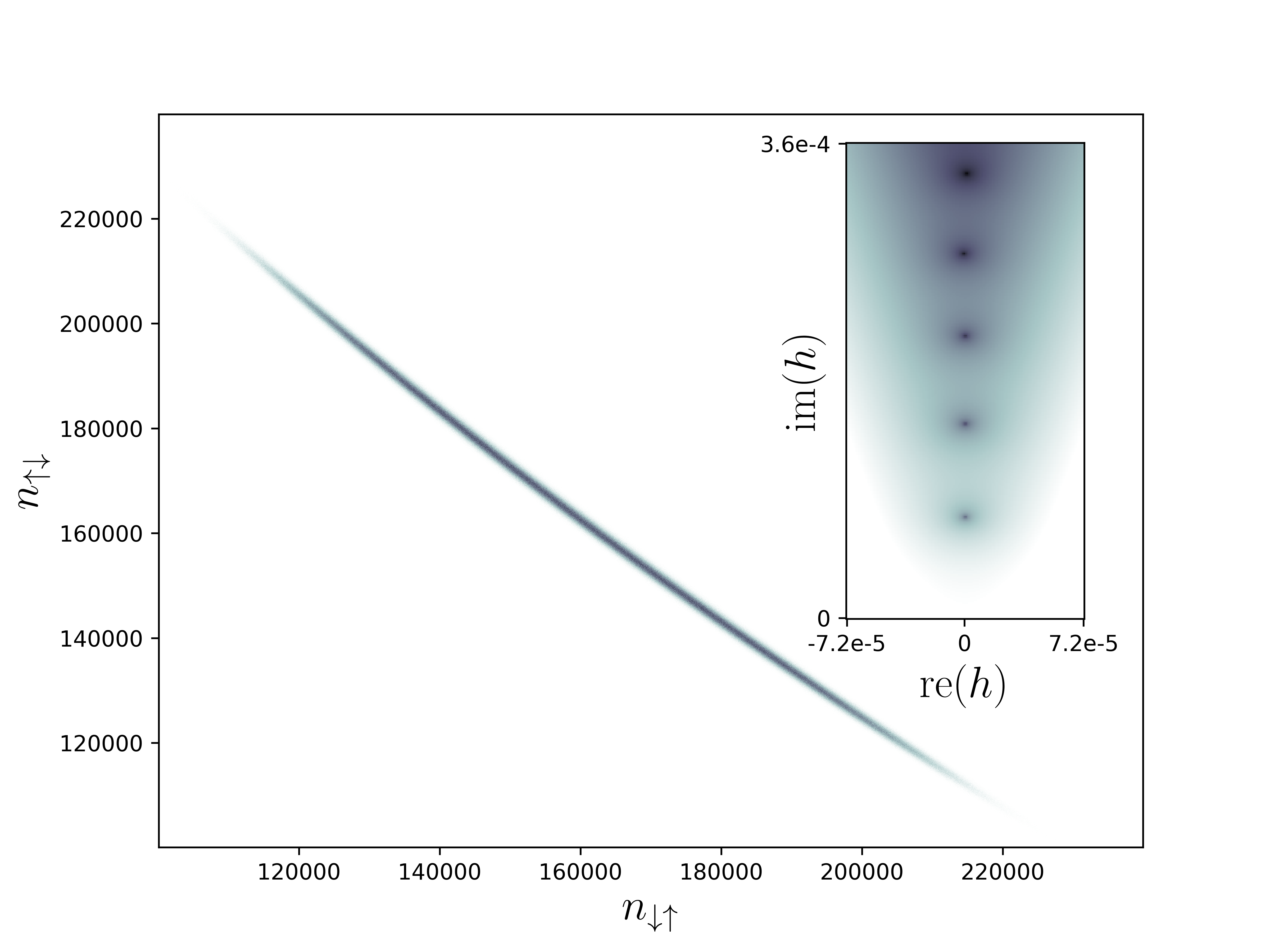
Figure 1: Main panel: A histogram of the number operators from Eq. (2) for the Heisenberg bilayer with $L=80$, $J_{\perp}=2.5222$ and $\beta=40$ with $J=1$. Inset: Eq. (2) applied to the histogram with complex-valued external Néel field $h$, where we plot $-\ln(|R_{0}(h)|)$ and the Lee-Yang zeros appear as the dark points.

Lee-Yang fields for quantum antiferromagnets: The classic case for Lee-Yang zeros is that of the Ising model in an external magnetic field, which is taken to be complex. The Lee-Yang circle theorem [Lee and Yang, 1952] then states that all of the Ising partition function zeros with a complex magnetic field lie on the imaginary axis. In order to extend this picture to quantum antiferromagnets we introduce a field that couples to the Néel order parameter. Here, remarkably, we will show that it is possible to compute the ratio at finite complex field while simulating the partition function in zero field.

The idea is to imagine embedding the $z-$component of the Néel field operator inside nearest-neighbor operators that are already present in the Hamiltonian $h_{i,j}=J(\vec{S}_{i}\cdot\vec{S}_{j}-\tfrac{1}{4})\to J(\vec{S}_{i}\cdot\vec{S}_{j}-\tfrac{1}{4})+\tfrac{h}{N_{c}}(S^{z}_{i}-S^{z}_{j})$. Here $i\in$ sublattice $A$ and $j\in$ sublattice $B$ and $N_{c}$ is the number of $J$-operators that touch each site (usually the coordination number of the lattice). The diagonal matrix elements then change as $-\langle\uparrow_{i}\downarrow_{j}|h_{i,j}|\uparrow_{i}\downarrow_{j}\rangle=\tfrac{J}{2}\to\tfrac{J}{2}-\tfrac{h}{N_{c}}$ and $-\langle\downarrow_{i}\uparrow_{j}|h_{i,j}|\downarrow_{i}\uparrow_{j}\rangle=\tfrac{J}{2}\to\tfrac{J}{2}+\tfrac{h}{N_{c}}$. The ratio of these matrix elements before and after the change gives $1\mp\frac{2h}{N_{c}J}$. If we denote the number of such matrix elements in an SSE configuration by $n_{\uparrow\downarrow}$ and $n_{\downarrow\uparrow}$ then the ratio formula with a Néel field reads

$$R_{0}(h)=\left\langle\left(1-\frac{2h}{N_{c}J}\right)^{n_{\uparrow\downarrow}}\left(1+\frac{2h}{N_{c}J}\right)^{n_{\downarrow\uparrow}}\right\rangle_{h=0}.$$ (2)

We emphasize that this formula only requires a histogram of the values $(n_{\uparrow\downarrow},n_{\downarrow\uparrow})$ obtained by QMC simulation (see Fig. (1)) of typical Heisenberg models in the absence of external fields, and allows for the statistically exact extraction of partition function zeros with a complex-valued Néel field. We now demonstrate this with a concrete example, the $O(3)$ quantum critical Heisenberg bilayer.

Heisenberg bilayer: As a first test case for this technique we select a well studied 2D quantum spin model for the $O(3)$ transition in $d=2+1$ dimensions, the Heisenberg bilayer given by the Hamiltonian

$$H_{\text{bl}}=J\sum_{\langle i,j\rangle,a=1,2}(\vec{S}_{i,a}\cdot\vec{S}_{j,a}-\tfrac{1}{4})+J_{\perp}\sum_{i}(\vec{S}_{i,1}\cdot\vec{S}_{i,2}-\tfrac{1}{4}),$$ (3)

where $\langle i,j\rangle$ are nearest neighbor pairs of a square lattice and $a$ is the layer index. When $J_{\perp}=0$ the model reduces to two independent Heisenberg models, which exhibits long-range Néel order at zero temperature, while for strong $J_{\perp}$ singlets are formed on the interlayer bonds and Néel order is destroyed. A continuous transition in the $O(3)$ universality class occurs at $J_{\perp}/J=2.5220(1)$ [Wang et al., 2006].

Here we will focus on extracting the Lee-Yang zeros, zeros of Eq. (2) at the critical point. First we show that the zeros of the partition function with a complex-valued Néel field lie exactly on the imaginary axis, akin to the Lee-Yang circle theorem for the Ising model [Lee and Yang, 1952] and its generalization to the classical Heisenberg model [Harris, 1970]. This is shown if Fig. (1), where in the main panel we display the histogram of the number operators from Eq. (2) that are used to compute the partition function ratio. The data is collected for a bilayer system with side length $L=80$ at the critical point, fixing $J=1,J_{\perp}=2.5222$ and $\beta=L/2$. The inset shows $-\ln(|R_{0}(h)|)$ computed with this histogram, where the dark spikes indicate the first five zeros near $|h|=0$, which lie directly on the imaginary axis.

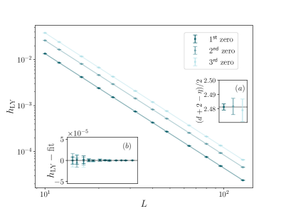
Figure 2: Main panel: The location on the imaginary axis of the first three Lee-Yang zeros of the Heisenberg bilayer in a complex Néel field at the critical point $J_{\perp}/J=2.5222$ and $\beta=L/2$. Panel (a): the exponent extracted from a fit of the data to the form $h_{\text{LY}}(L)\sim L^{-(d+2-\eta)/2}(1+bL^{-\omega})$, where the fit is performed separately for each of the first three zeros. The grey line is the best estimate of the exponent from the literature [Campostrini et al., 2002]. Panel (b): the raw data minus the fit.

Now we investigate the critical scaling of the leading zeros of the Heisenberg bilayer as we approach the thermodynamic limit, using finite-size scaling of the location of the zeros to extract critical exponents. At a critical point, Lee-Yang zeros are expected to scale as $h_{\text{LY}}(L)\sim L^{-\beta\delta/\nu}$ [Itzykson et al., 1983], where, through scaling relations, the exponent can be expressed as $\beta\delta/\nu=(d+2-\eta)/2$. For the Heisenberg bilayer, we find it necessary to include corrections to scaling of the form $h_{\text{LY}}(L)\sim L^{-(d+2-\eta)/2}(1+bL^{-\omega})$, as has been previously observed with Lee-Yang zeros for the 3D classical Heisenberg model [Gordillo-Guerrero et al., 2013]. Fig. (2) shows the first three zeros extracted from bilayer systems collected at $J=1,J_{\perp}=2.5222$ and $\beta=L/2$. The extracted exponent is given in inset $(a)$, which agrees perfectly with the best estimate from classical Monte Carlo simulations [Campostrini et al., 2002]. Interestingly, we also find the correction to scaling $\omega\approx 1$ in agreement with the classical case [Gordillo-Guerrero et al., 2013].

Deconfined criticality: Now that we have demonstrated the ability to extract critical exponents from the finite-size scaling of Lee-Yang zeros for the first time at a quantum critical point, we move on to a more exotic quantum spin model that shows criticality and emergent symmetry between two seemingly unrelated order parameters.

The $J$-$Q$ model [Sandvik, 2007] is given by the following Hamiltonian:

$$H_{JQ}=J\sum_{\langle i,j\rangle}(\vec{S}_{i}\cdot\vec{S}_{j}-\tfrac{1}{4})-Q\sum_{\langle i,j,k,l\rangle}(\vec{S}_{i}\cdot\vec{S}_{j}-\tfrac{1}{4})(\vec{S}_{k}\cdot\vec{S}_{l}-\tfrac{1}{4}),$$ (4)

where $J$ is the nearest-neighbor coupling on a square lattice and $Q$ is a four-spin interaction that acts on elementary plaquettes of the square lattice. $Q$ can be thought of as a product of two $J$’s and the sum over $\langle i,j,k,l\rangle$ includes both $\hat{x}$ and $\hat{y}$ orientations to preserve lattice symmetries. When $Q=0$ the $J$-$Q$ model reduces to the Heisenberg antiferromagnet, which exhibits long-range Néel order at $T=0$. However, for large $Q$, magnetic order is destroyed by locally forming singlets that stack along columns of the square lattice, referred to as valence-bond solid (VBS) order, which breaks lattice translation symmetry. At $J/Q\approx 0.045$ the system undergoes a seemingly continuous transition between these two distinct ordered phases, which belongs to a class of transitions known as deconfined quantum critical points (DQCP) [Senthil et al., 2004a, Senthil et al., 2004b].

The true nature of the phase transition in the $J$-$Q$ model has been the topic of continued debate. While most studies observe a direct continuous transition between Néel and VBS order [Sandvik, 2007; Lou et al., 2009; Sandvik, 2010b; Harada et al., 2013; Block et al., 2013; Shao et al., 2016; Sandvik and Zhao, 2020; Zhao et al., 2020], other studies show evidence of a weak first-order transition [Kuklov et al., 2008; Jiang et al., 2008; Chen et al., 2013; D’Emidio et al., 2021; Zhao et al., 2022; Song et al., 2023]. The $J$-$Q$ model therefore provides us with an important case for the study of Lee-Yang zeros.

Having already developed the methodology to extract Lee-Yang zeros associated with fluctuations of the Néel order parameter, we would now like to develop an analogous treatment for the VBS order parameter. Here we must introduce a complex-valued field that couples to the VBS order parameter, which is a field that preserves spin rotation symmetry but breaks lattice translation symmetry. In order to do so, we make use of the $Q$ plaquette terms that are already present in the Hamiltonian, and we introduce the field $d\sum_{\langle i,j,k,l\rangle\in\hat{x}_{e}}P_{i,j,k,l}-d\sum_{\langle i,j,k,l\rangle\in\hat{x}_{o}}P_{i,j,k,l}$ where $P_{i,j,k,l}\equiv(\vec{S}_{i}\cdot\vec{S}_{j}-\tfrac{1}{4})(\vec{S}_{k}\cdot\vec{S}_{l}-\tfrac{1}{4})$ and $\hat{x}_{e}$ are all $\hat{x}$-oriented plaquettes on even columns of the square lattice and $\hat{x}_{o}$ are all $\hat{x}$-oriented plaquettes on odd columns. $d$ is the coupling strength of the VBS field, which we will take to be complex-valued.

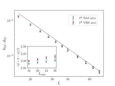
Figure 3: Main panel: the locations of the first Lee-Yang zeros in the $J$-$Q$ model at the critical point in two separate cases: with a complex Néel field and with a complex VBS field. The thin black line shows the power law behavior expected at a first order transition with $\eta=0$. Inset: The fitted exponent from a simple power law fit of the zeros to the form $\sim L^{-(d+2-\eta)/2}$ as a function of the smallest system size used in the fit.

Following the same prescription as the ratio formula with a complex Néel field, we have the ratio with a complex VBS field as follows:

$$R_{0}(d)=\left\langle\left(1-\frac{d}{Q}\right)^{n_{Q_{xe}}}\left(1+\frac{d}{Q}\right)^{n_{Q_{xo}}}\right\rangle_{d=0}.$$ (5)

Here $n_{Q_{xe}}$ is the number $\hat{x}$-oriented $Q$ matrix elements on even columns of the square lattice and $n_{Q_{xo}}$ is the same but for odd columns. Again, we only require a histogram of the values $(n_{Q_{xe}},n_{Q_{xo}})$ obtained from QMC simulation of the pure $J$-$Q$ model without any fields, and Eqn. (5) allows for the statistically exact extraction of Lee-Yang zeros of the partition function with a complex VBS field. For the $J$-$Q$ model we can simultaneously gather histograms for both the Néel zeros and VBS zeros in a single simulation.

In Fig. (3) we plot the location of the Lee-Yang zeros $h_{\text{LY}},d_{\text{LY}}$ as a function of system size at the critical point $J=0.04502$, $Q=1$ with $\beta=L/2$. Indeed, as with the Néel zeros, we find the nearest VBS zeros lie exactly on the imaginary axis: re$(h_{\text{LY}})=$ re$(d_{\text{LY}})=0$. For simplicity we plot only the location of the leading zeros. In the $J$-$Q$ model, contrary to the Heisenberg bilayer, we achieve much better fits using only a simple power law with no corrections to scaling. The extracted exponents are far below the values of the bilayer, signaling a much larger value of $\eta$ here, with our values in the range of previous studies. We do, however, observe drifting of the critical exponents, as shown in the inset, which is also similar to what was observed in other studies [Harada et al., 2013, Nahum et al., 2015].

Combined Néel and VBS fields: The transition in the $J$-$Q$ model is frequently described in terms of an emergent SO(5) symmetry that arises between the Néel and VBS order parameters exactly at the critical point. From this point of view, it is interesting to ask the how the zeros of the partition function are distributed in the presence of combined Néel and VBS fields. Fortunately, our formulation allows us to simply compute the ratio when both fields are nonzero, again, while the actual simulation is carried out in zero field. We can straightforwardly define the combined ratio as:

$$\begin{split}R_{0}(h,d)&=\left\langle\left(1-\frac{2h}{N_{c}J}\right)^{n_{\uparrow\downarrow}}\left(1+\frac{2h}{N_{c}J}\right)^{n_{\downarrow\uparrow}}\right.\\ &\left.\quad\quad\left(1-\frac{d}{Q}\right)^{n_{Q_{xe}}}\left(1+\frac{d}{Q}\right)^{n_{Q_{xo}}}\right\rangle_{h=0,d=0}.\end{split}$$ (6)

In Fig. (4) we plot $-\ln(|R_{0}(h,d)|)$ for purely imaginary values of $h$ and $d$ at the critical point. Interestingly, we see that the partition function zeros form extended rings in the plane (im($h$),im($d$)). On either side of the transition the ovals become elongated in either the vertical or horizontal direction (see supplemental materials). Our conclusion is that at the critical point these rings shrink down to the origin in the thermodynamic limit, whereas on either side of the transition they become squashed in either the horizontal or vertical direction. It is interesting to note that although the values of $J$ and $Q$ differ by an order of magnitude at the transition, the lines of zeros are nearly circular in terms of $h$ and $d$.

Conclusions: We have presented the first large-scale QMC computations of Lee-Yang zeros in quantum spin systems. Our formulation is simple to implement, in that it only requires gathering a histogram of the number of certain types of matrix elements that appear during standard QMC simulations in the absence of any external fields. Furthermore, we find that the location of Lee-Yang zeros computed in this way is extremely precise, easily allowing for the extraction of the the first three zeros for the critical Heisenberg bilayer on system sizes up to $L=128$ and excellent agreement with known critical exponents. We also have demonstrated the generality of this approach by using it to extract Lee-Yang zeros associated with critical Néel, VBS and combined Néel-VBS fluctuations in the $J$-$Q$ model, the emblematic model of deconfined criticality.

Moving forward, we envision that this technique could be applied to extract properties of non-unitary critical points that occur at finite imaginary field values. Specifically, with the partition function ratio in hand, it allows one to compute expectation values in the ensemble with a complex field. This seems promising given that the ratio is computed to high precision in this framework. On a speculative note, these types of studies could aid in understanding lattice models with pseudo-critical behavior, where the true critical point lies in the complex plane but with a small imaginary component, as has been proposed to explain anomalous behavior in models of deconfined criticality [Nahum et al., 2015; Gorbenko et al., 2018; Ma and Wang, 2020; Nahum, 2020; Song et al., 2023].

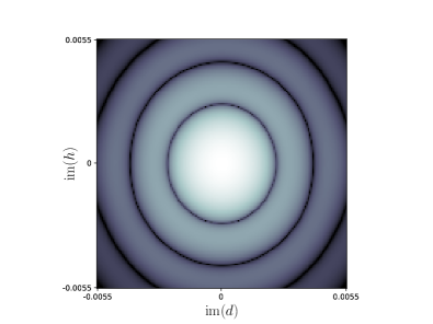
Figure 4: A density plot of $-\ln(|R_{0}(h,d)|)$ for the $J$-$Q$ model at the critical coupling with $L=32$. The dark lines indicate zeros of the partition function in the $J$-$Q$ model subjected to combined Néel and VBS fields.

Acknowledgements: We thank Román Orús for his support for this project. Computing resources were used from the XSEDE allocation NSF DMR-130040 using the Expanse cluster at the San Diego Supercomputer Center.

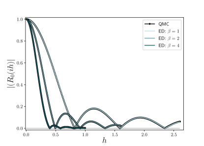
Figure 5: A comparison of data obtained with the QMC method versus exact diagonalization. The system is an $L=2$ Heisenberg bilayer with $J=1,J_{\perp}=2.52205$ with three different values of $\beta$. The ratio $|R_{0}(h)|$ is plotted as a function of the Néel field $h$ along the imaginary axis.

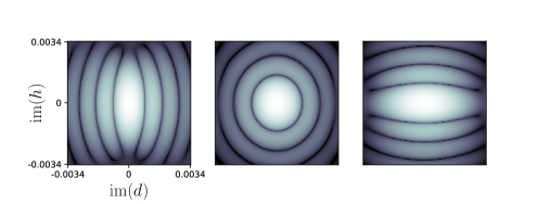
Figure 6: A density plot of $-\ln(|R_{0}(h,d)|)$ for the $J$-$Q$ model at the critical coupling with $L=40$ at three different values of the coupling: $J/Q=0.015,0.045,0.085$ from left to right.

I Supplemental material

I.1 QMC versus exact diagonalization

Here we demonstrate the validity of Eqn. (2) by comparing against exact results for a small system size. Fig. (5) shows $|R_{0}(h)|$ computed with a purely imaginary Néel field on a $2\times 2$ Heisenberg bilayer system compared against exact diagonalization of the whole spectrum. We make the comparison for three different values of $\beta$, where in each case the first three Lee-Yang zeros are visible. The QMC values match the exact results perfectly within the statistical uncertainty.

I.2 Data away from deconfined critical point

Here we would like to show what happens to the nearly circular distribution of zeros, with combined imaginary Néel and VBS fields, away from the critical point in the $J$-$Q$ model. In Fig. (6) we show density plots (similar to Fig. (4)) for three different values of the coupling: $J/Q=0.015,0.045,0.085$ from left to right for system size $L=40$. Here we see on the left, which is on the VBS side of the transition, the Néel zeros get pushed away from the origin, relative to their values at the transition given, and in fact are not clearly detectable on this plot. A similar story goes for the right panel. While we believe our data to be statistically converged for the field values shown, which would indicate a potential rearrangement of the lines of zeros away from the critical point, we cannot rule out the possibility of under sampling at the larger field values.

References

- Yang and Lee (1952) C. N. Yang and T. D. Lee, “Statistical theory of equations of state and phase transitions. i. theory of condensation,” Phys. Rev. 87, 404–409 (1952).
- Lee and Yang (1952) T. D. Lee and C. N. Yang, “Statistical theory of equations of state and phase transitions. ii. lattice gas and ising model,” Phys. Rev. 87, 410–419 (1952).
- Fisher (1978) Michael E. Fisher, “Yang-lee edge singularity and field theory,” Phys. Rev. Lett. 40, 1610–1613 (1978).
- Cardy (1985) John L. Cardy, “Conformal invariance and the yang-lee edge singularity in two dimensions,” Phys. Rev. Lett. 54, 1354–1356 (1985).
- Binek (1998) Ch. Binek, “Density of zeros on the lee-yang circle obtained from magnetization data of a two-dimensional ising ferromagnet,” Phys. Rev. Lett. 81, 5644–5647 (1998).
- Peng et al. (2015) Xinhua Peng, Hui Zhou, Bo-Bo Wei, Jiangyu Cui, Jiangfeng Du, and Ren-Bao Liu, “Experimental observation of lee-yang zeros,” Phys. Rev. Lett. 114, 010601 (2015).
- Brandner et al. (2017) Kay Brandner, Ville F. Maisi, Jukka P. Pekola, Juan P. Garrahan, and Christian Flindt, “Experimental determination of dynamical lee-yang zeros,” Phys. Rev. Lett. 118, 180601 (2017).
- Francis et al. (2021) Akhil Francis, Daiwei Zhu, Cinthia Huerta Alderete, Sonika Johri, Xiao Xiao, James K. Freericks, Christopher Monroe, Norbert M. Linke, and Alexander F. Kemper, “Many-body thermodynamics on quantum computers via partition function zeros,” Science Advances 7, eabf2447 (2021), https://www.science.org/doi/pdf/10.1126/sciadv.abf2447 .
- Lee (2013) Julian Lee, “Exact partition function zeros of the wako-saitô-muñoz-eaton protein model,” Phys. Rev. Lett. 110, 248101 (2013).
- Deger et al. (2018) Aydin Deger, Kay Brandner, and Christian Flindt, “Lee-yang zeros and large-deviation statistics of a molecular zipper,” Phys. Rev. E 97, 012115 (2018).
- Majumdar and Bhattacharjee (2020) Debjyoti Majumdar and Somendra M. Bhattacharjee, “Zeros of partition function for continuous phase transitions using cumulants,” Physica A: Statistical Mechanics and its Applications 553, 124263 (2020).
- Nagata et al. (2015) Keitaro Nagata, Kouji Kashiwa, Atsushi Nakamura, and Shinsuke M. Nishigaki, “Lee-yang zero distribution of high temperature qcd and the roberge-weiss phase transition,” Phys. Rev. D 91, 094507 (2015).
- Bena et al. (2005) Ioana Bena, Michel Droz, and Adam Lipowski, “Statistical mechanics of equilibrium and nonequilibrium phase transitions: The yang–lee formalism,” International Journal of Modern Physics B 19, 4269–4329 (2005), https://doi.org/10.1142/S0217979205032759 .
- Ferrenberg and Swendsen (1988) Alan M. Ferrenberg and Robert H. Swendsen, “New monte carlo technique for studying phase transitions,” Phys. Rev. Lett. 61, 2635–2638 (1988).
- Kenna and Lang (1993) R. Kenna and C.B. Lang, “Lee-yang zeroes and logarithmic corrections in the theory,” Nuclear Physics B - Proceedings Supplements 30, 697–700 (1993), proceedings of the International Symposium on.
- Kenna and Lang (1994) R. Kenna and C. B. Lang, “Scaling and density of lee-yang zeros in the four-dimensional ising model,” Phys. Rev. E 49, 5012–5017 (1994).
- Flindt and Garrahan (2013) Christian Flindt and Juan P. Garrahan, “Trajectory phase transitions, lee-yang zeros, and high-order cumulants in full counting statistics,” Phys. Rev. Lett. 110, 050601 (2013).
- Deger et al. (2020) Aydin Deger, Fredrik Brange, and Christian Flindt, “Lee-yang theory, high cumulants, and large-deviation statistics of the magnetization in the ising model,” Phys. Rev. B 102, 174418 (2020).
- Shimizu and Kuramashi (2014a) Yuya Shimizu and Yoshinobu Kuramashi, “Grassmann tensor renormalization group approach to one-flavor lattice schwinger model,” Phys. Rev. D 90, 014508 (2014a).
- Shimizu and Kuramashi (2014b) Yuya Shimizu and Yoshinobu Kuramashi, “Critical behavior of the lattice schwinger model with a topological term at using the grassmann tensor renormalization group,” Phys. Rev. D 90, 074503 (2014b).
- García-Saez and Wei (2015) Artur García-Saez and Tzu-Chieh Wei, “Density of yang-lee zeros in the thermodynamic limit from tensor network methods,” Phys. Rev. B 92, 125132 (2015).
- Hong and Kim (2022) Seongpyo Hong and Dong-Hee Kim, “Tensor network calculation of the logarithmic correction exponent in the xy model,” Journal of the Physical Society of Japan 91, 084003 (2022), https://doi.org/10.7566/JPSJ.91.084003 .
- Heyl et al. (2013) M. Heyl, A. Polkovnikov, and S. Kehrein, “Dynamical quantum phase transitions in the transverse-field ising model,” Phys. Rev. Lett. 110, 135704 (2013).
- Ananikian et al. (2014) N.S. Ananikian, V.V. Hovhannisyan, and R. Kenna, “Partition function zeros of the antiferromagnetic spin-12 ising–heisenberg model on a diamond chain,” Physica A: Statistical Mechanics and its Applications 396, 51–60 (2014).
- Peotta et al. (2021) Sebastiano Peotta, Fredrik Brange, Aydin Deger, Teemu Ojanen, and Christian Flindt, “Determination of dynamical quantum phase transitions in strongly correlated many-body systems using loschmidt cumulants,” Phys. Rev. X 11, 041018 (2021).
- Kist et al. (2021) Timo Kist, Jose L. Lado, and Christian Flindt, “Lee-yang theory of criticality in interacting quantum many-body systems,” Phys. Rev. Res. 3, 033206 (2021).
- Vecsei et al. (2022) Pascal M. Vecsei, Jose L. Lado, and Christian Flindt, “Lee-yang theory of the two-dimensional quantum ising model,” Phys. Rev. B 106, 054402 (2022).
- Brange et al. (2022) Fredrik Brange, Sebastiano Peotta, Christian Flindt, and Teemu Ojanen, “Dynamical quantum phase transitions in strongly correlated two-dimensional spin lattices following a quench,” Phys. Rev. Res. 4, 033032 (2022).
- Vecsei et al. (2023) Pascal M. Vecsei, Christian Flindt, and Jose L. Lado, “Lee-yang theory of quantum phase transitions with neural network quantum states,” (2023), arXiv:2301.09923 [cond-mat.str-el] .
- Sandvik (2010a) Anders W. Sandvik, “Computational studies of quantum spin systems,” AIP Conference Proceedings 1297, 135–338 (2010a), https://aip.scitation.org/doi/pdf/10.1063/1.3518900 .
- Wang et al. (2006) Ling Wang, K. S. D. Beach, and Anders W. Sandvik, “High-precision finite-size scaling analysis of the quantum-critical point of heisenberg antiferromagnetic bilayers,” Phys. Rev. B 73, 014431 (2006).
- Harris (1970) A.Brooks Harris, “Generalizations of the lee-yang theorem,” Physics Letters A 33, 161–162 (1970).
- Campostrini et al. (2002) Massimo Campostrini, Martin Hasenbusch, Andrea Pelissetto, Paolo Rossi, and Ettore Vicari, “Critical exponents and equation of state of the three-dimensional heisenberg universality class,” Phys. Rev. B 65, 144520 (2002).
- Itzykson et al. (1983) C. Itzykson, R.B. Pearson, and J.B. Zuber, “Distribution of zeros in ising and gauge models,” Nuclear Physics B 220, 415–433 (1983).
- Gordillo-Guerrero et al. (2013) A. Gordillo-Guerrero, R. Kenna, and J. J. Ruiz-Lorenzo, “Scaling behavior of the heisenberg model in three dimensions,” Phys. Rev. E 88, 062117 (2013).
- Sandvik (2007) Anders W. Sandvik, “Evidence for deconfined quantum criticality in a two-dimensional heisenberg model with four-spin interactions,” Phys. Rev. Lett. 98, 227202 (2007).
- Senthil et al. (2004a) T. Senthil, Ashvin Vishwanath, Leon Balents, Subir Sachdev, and Matthew P. A. Fisher, “Deconfined quantum critical points,” Science 303, 1490–1494 (2004a), https://www.science.org/doi/pdf/10.1126/science.1091806 .
- Senthil et al. (2004b) T. Senthil, Leon Balents, Subir Sachdev, Ashvin Vishwanath, and Matthew P. A. Fisher, “Quantum criticality beyond the landau-ginzburg-wilson paradigm,” Phys. Rev. B 70, 144407 (2004b).
- Lou et al. (2009) Jie Lou, Anders W. Sandvik, and Naoki Kawashima, “Antiferromagnetic to valence-bond-solid transitions in two-dimensional heisenberg models with multispin interactions,” Phys. Rev. B 80, 180414 (2009).
- Sandvik (2010b) Anders W. Sandvik, “Continuous quantum phase transition between an antiferromagnet and a valence-bond solid in two dimensions: Evidence for logarithmic corrections to scaling,” Phys. Rev. Lett. 104, 177201 (2010b).
- Harada et al. (2013) Kenji Harada, Takafumi Suzuki, Tsuyoshi Okubo, Haruhiko Matsuo, Jie Lou, Hiroshi Watanabe, Synge Todo, and Naoki Kawashima, “Possibility of deconfined criticality in su() heisenberg models at small ,” Phys. Rev. B 88, 220408 (2013).
- Block et al. (2013) Matthew S. Block, Roger G. Melko, and Ribhu K. Kaul, “Fate of fixed points with monopoles,” Phys. Rev. Lett. 111, 137202 (2013).
- Shao et al. (2016) Hui Shao, Wenan Guo, and Anders W. Sandvik, “Quantum criticality with two length scales,” Science 352, 213–216 (2016), https://www.science.org/doi/pdf/10.1126/science.aad5007 .
- Sandvik and Zhao (2020) Anders W. Sandvik and Bowen Zhao, “Consistent scaling exponents at the deconfined quantum-critical point*,” Chinese Physics Letters 37, 057502 (2020).
- Zhao et al. (2020) Bowen Zhao, Jun Takahashi, and Anders W. Sandvik, “Multicritical deconfined quantum criticality and lifshitz point of a helical valence-bond phase,” Phys. Rev. Lett. 125, 257204 (2020).
- Kuklov et al. (2008) A. B. Kuklov, M. Matsumoto, N. V. Prokof’ev, B. V. Svistunov, and M. Troyer, “Deconfined criticality: Generic first-order transition in the su(2) symmetry case,” Phys. Rev. Lett. 101, 050405 (2008).
- Jiang et al. (2008) F-J Jiang, M Nyfeler, S Chandrasekharan, and U-J Wiese, “From an antiferromagnet to a valence bond solid: evidence for a first-order phase transition,” Journal of Statistical Mechanics: Theory and Experiment 2008, P02009 (2008).
- Chen et al. (2013) Kun Chen, Yuan Huang, Youjin Deng, A. B. Kuklov, N. V. Prokof’ev, and B. V. Svistunov, “Deconfined criticality flow in the heisenberg model with ring-exchange interactions,” Phys. Rev. Lett. 110, 185701 (2013).
- D’Emidio et al. (2021) Jonathan D’Emidio, Alexander A. Eberharter, and Andreas M. Läuchli, “Diagnosing weakly first-order phase transitions by coupling to order parameters,” (2021), arXiv:2106.15462 [cond-mat.str-el] .
- Zhao et al. (2022) Jiarui Zhao, Yan-Cheng Wang, Zheng Yan, Meng Cheng, and Zi Yang Meng, “Scaling of entanglement entropy at deconfined quantum criticality,” Phys. Rev. Lett. 128, 010601 (2022).
- Song et al. (2023) Menghan Song, Jiarui Zhao, Lukas Janssen, Michael M. Scherer, and Zi Yang Meng, “Deconfined quantum criticality lost,” (2023), arXiv:2307.02547 [cond-mat.str-el] .
- Nahum et al. (2015) Adam Nahum, J. T. Chalker, P. Serna, M. Ortuño, and A. M. Somoza, “Deconfined quantum criticality, scaling violations, and classical loop models,” Phys. Rev. X 5, 041048 (2015).
- Gorbenko et al. (2018) Victor Gorbenko, Slava Rychkov, and Bernardo Zan, “Walking, weak first-order transitions, and complex cfts,” Journal of High Energy Physics 2018, 108 (2018).
- Ma and Wang (2020) Ruochen Ma and Chong Wang, “Theory of deconfined pseudocriticality,” Phys. Rev. B 102, 020407 (2020).
- Nahum (2020) Adam Nahum, “Note on wess-zumino-witten models and quasiuniversality in dimensions,” Phys. Rev. B 102, 201116 (2020).