PVG: Progressive Vision Graph for Vision Recognition

Abstract.

Convolution-based and Transformer-based vision backbone networks process images into the grid or sequence structures, respectively, which are inflexible for capturing irregular objects. Though Vision GNN (ViG) adopts graph-level features for complex images, it has some issues, such as inaccurate neighbor node selection, expensive node information aggregation calculation, and over-smoothing in the deep layers. To address the above problems, we propose a Progressive Vision Graph (PVG) architecture for vision recognition task. Compared with previous works, PVG contains three main components: 1) Progressively Separated Graph Construction (PSGC) to introduce second-order similarity by gradually increasing the channel of the global graph branch and decreasing the channel of local branch as the layer deepens; 2) Neighbor nodes information aggregation and update module by using Max pooling and mathematical Expectation (MaxE) to aggregate rich neighbor information; 3) Graph error Linear Unit (GraphLU) to enhance low-value information in a relaxed form to reduce the compression of image detail information for alleviating the over-smoothing. Extensive experiments on mainstream benchmarks demonstrate the superiority of PVG over state-of-the-art methods, e.g., our PVG-S obtains 83.0% Top-1 accuracy on ImageNet-1K that surpasses GNN-based ViG-S by +0.9$\uparrow$ with the parameters reduced by 18.5%, while the largest PVG-B obtains 84.2% that has +0.5$\uparrow$ improvement than ViG-B. Furthermore, our PVG-S obtains +1.3$\uparrow$ box AP and +0.4$\uparrow$ mask AP gains than ViG-S on COCO dataset.

1. Introduction

The Convolutional Neural Network (CNN) (LeCun et al., 1998) has been the dominant approach for general Computer Vision (CV) tasks (Li et al., 2019b, 2021b) due to its powerful inductive bias for capturing local information (Simonyan and Zisserman, 2014; Krizhevsky et al., 2017; Szegedy et al., 2015; He et al., 2016). However, the recent introduction of the transformer with attention mechanism from Natural Language Processing (NLP) into CV by ViT (Dosovitskiy et al., 2020) has shown that the vision transformer can achieve better performance than CNN with a large amount of pre-training. Subsequent ViT-based works (Liu et al., 2021a; Wang et al., 2021; Liu et al., 2022a; Dong et al., 2022; Li et al., 2022b; Zhang et al., 2022, 2021, 2023) further demonstrate the powerful capabilities of the transformer in various downstream tasks, such as object detection (Wu et al., 2023) and segmentation (Li et al., 2022c; Han et al., 2023). The studies have expedited the trend of unifying the Transformer architecture in the fields of NLP and CV.

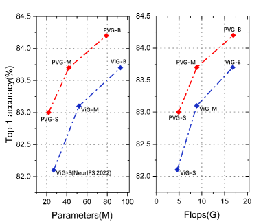
Figure 1. The comparison of Accuracy vs. Parameters and FLOPs between PVG and ViG. Our PVG achieves the best balance between accuracy and computation on the Imagenet.

However, the above CNNs and Transformers are designed to handle regular grid data (e.g., images) or sequential data (e.g., text) and are not flexible enough to capture non-Euclidean graph-structured data. To address this challenge, researchers have proposed a number of graph neural networks (GNN) technologies (Bruna et al., 2013; Defferrard et al., 2016; Levie et al., 2018; Niepert et al., 2016; Veličković et al., 2017; Monti et al., 2017). Since real-world objects often have irregular structures and various sizes, images can be viewed as a graph composition of parts. Some advanced graph-based approaches (Chen et al., 2019a; You et al., 2020; Yang et al., 2020; Ma et al., 2019; Roy et al., 2021) have been proposed for visual recognition. In addition, various GNN methods have been proposed for various downstream tasks, such as point cloud (Li et al., 2019a), object detection (Zhao et al., 2021), and segmentation (Wu et al., 2020). Moreover, some graph-based works (Chen et al., 2019b, 2020, c; Wang et al., 2020) achieve competitive results in language processing tasks. Given these advancements, it is reasonable to ask whether GNN can serve as the backbone of computer vision and become a strong contender for the unified architecture of image, language, and graph-structured data in the future.

ViG (Han et al., 2022) is the pioneering work in the field of computer vision that uses Vision Graph Neural Network (GNN) to process images. The model divides the input image into several patches and treats each patch as a node to enable information interaction. Despite significant progress, ViG still faces several challenges that remain unaddressed. ViG constructs graphs for images using only simple first-order similarity, which can result in inaccurate selection and connections among neighbor nodes. For graph information interaction, ViG applies two advanced Graph node information update functions in the GNN field: MR GraphConv (Li et al., 2019a), which has the lowest computational burden but poor performance, and EdgeConv (Wang et al., 2019), which performs well but has a high computational burden. Therefore, a node aggregation and an update function that can balance computation and performance well is needed. Additionally, ViG still experiences over-smoothing issues (Li et al., 2019a) in deep layers. As the GNN goes deeper, the node representations become similar or even identical after certain layers, leading to a loss of information and reduced performance.

Towards the problems above, in this paper, we propose a new vision GNN architecture called Progressive Vision Graph (PVG) for general-purpose vision tasks. Fig. 2 illustrates our PVG structure design, which follows previous pyramid principles (Wang et al., 2021) and is designed in a cascaded four-stage manner, with each stage composed of several graph blocks. Fig. 2 also highlights three key contributions of our PVG. Our first contribution is Progressively Separated Graph Construction (PSGC), which captures crucial second-order similarity information without increasing computation cost. PSGC splits the vision graph into three graphs constructed from different similarity measures in the channel dimension. In the shallow layer, we allocate a small part of the channel to the global graph. As the layer deepens, the channel ratio of the global graph gradually increases, fully absorbing the local information obtained from the local branch. This process calculates the second-order similarity of the nodes’ features, which is equivalent to the similarity of their neighbors. PSGC is the first method to generalize the second-order similarity (Wang et al., 2016), an important concept in the GNN field, to vision tasks. The whole process is computationally efficient and does not introduce additional costs. We also propose a new node information aggregation and update method called MaxE, which is based on the distribution of neighbor representations. MaxE consists of three parts: node self-representation, the mathematical expectation of neighbor nodes, and the maximum Euclidean distance between the central node and its neighbor. Our experiments show that the proposed MaxE is effective and efficient, achieving the same performance as the powerful EdgeConv (Wang et al., 2019) while reducing the number of parameters by 70%. To address the over-smoothing problem, we propose GraphLU, a simple yet effective method that regenerates the node features to increase their diversity at deep layers with minimal computation and memory cost. GraphLU is a concise activation function that can be generalized to various computer vision backbone networks. Our proposed PVG achieves significant performance gains compared to the advanced graph-based backbone ViG (Han et al., 2022), while reducing the model parameters by around 20%. Fig. 1 illustrates the performance improvement of PVG over VIG. To summarise, the main contributions of this paper are as follows:

• PSGC method introduces the important second-order similarity concept from the GNN field into the computer vision, providing more accurate neighbor node selection;

• A novel graph node aggregation and update mechanism MaxE to obtains state-of-the-art performance and low computation cost for vision tasks;

• An improved concise activation function GraphLU to solve the over-smoothing in the deep layers of Vision GNN without any addition computation cost;

• Our proposed PVG accelerates the generalization progress of Graph Neural Network (GNN) to Computer Vision (CV).

2. Related Work

2.1. CNN and Transformer for Vision

Convolutional neural networks (CNNs) have been highly successful in modeling local dependencies, making them the leading approach in computer vision since the introduction of AlexNet (Krizhevsky et al., 2017). Over time, researchers have developed increasingly effective CNN architectures, including VGG (Simonyan and Zisserman, 2014), GoogleNet (Szegedy et al., 2015), ResNet (He et al., 2016), MobileNet (Howard et al., 2017), and others, which have further propelled the field forward.

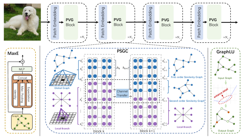
Figure 2. Our PVG architecture is designed in a cascaded four-stage manner, with each stage adopting the Progressively Separated Graph Construction (PSGC) to introduce second-order similarity, which transfers channels from local to global graphs between adjacent blocks. After graph construction, PVG uses our proposed MaxE in each block for information aggregation and update. Additionally, PVG utilizes a concise activation function GraphLU to enhance detail for alleviating the over-smoothing problem.

However, the introduction of ViT (Dosovitskiy et al., 2020) has challenged the dominance of CNNs in computer vision. Subsequent works, such as Deit (Touvron et al., 2021), PVT (Wang et al., 2021), T2T (Yuan et al., 2021) and Swin (Liu et al., 2021a), have achieved impressive performance in various downstream vision tasks. Additionally, some research efforts have proposed novel hybrid structures, such as CvT (Wu et al., 2021), Coatnet (Dai et al., 2021), Container (Gao et al., 2021), and ViTAE (Xu et al., 2021), which leverage the strengths of both CNN and Transformer models. These efforts elevate the field of computer vision to a higher level. Recently, some works make attempts to strike back at Transformer architecture in computer vision by designing advanced pure CNN architectures, such as ConvNeXt (Liu et al., 2022b) and RepLKNet (Ding et al., 2022), which show competitive results across various vision tasks and are faster than Transformer models in inference.

2.2. Graph Neural Network

There are two main branches of graph neural network research for non-European graph data: frequency domain graph convolution (Bruna et al., 2013; Henaff et al., 2015; Defferrard et al., 2016; Kipf and Welling, 2016; Levie et al., 2018; Li et al., 2018b) and spatial domain convolution (Atwood and Towsley, 2016; Niepert et al., 2016; Hamilton et al., 2017; Veličković et al., 2017; Monti et al., 2017; Huang et al., 2018). Representative works that improve GNN performance by enabling convolution operations on non-Euclidean datasets, including ChebNet (Defferrard et al., 2016), GCNs(Kipf and Welling, 2016), GraphSAGE (Hamilton et al., 2017) and GAT (Veličković et al., 2017). Furtherly, DeepGCNs (Li et al., 2019a) introduces concepts from CNNs such as residual structure and dilated convolution, into GNNs, realizing a 56-layer graph convolution network. Subsequent works including Mixhop (Abu-El-Haija et al., 2019), GDC (Gasteiger et al., 2019), and S2GC (Zhu and Koniusz, 2021), have further extended the depth and generalization capabilities of GNNs for graph data such as social network and biochemical graphs.

GNNs have been extensively applied in computer vision tasks, such as few-shot learning and zero-shot learning (Chen et al., 2019a; You et al., 2020; Yang et al., 2020; Kampffmeyer et al., 2019; Liu et al., 2021b). They have also facilitated advancements in domain adaptation and generalization (Ma et al., 2019; Roy et al., 2021; Luo et al., 2020; Chen et al., 2022). In addition, some works have also utilized GNNs to enhance the features of the CNN backbone in object detection tasks (Zhao et al., 2021; Li et al., 2022a; Zhang et al., 2020), perform graph reasoning on class pixels (Hu et al., 2020), and design bidirectional graph reasoning networks for panoramic segmentation (Wu et al., 2020). Few works have directly utilized GNNs as the backbone network for computer vision. ViG (Han et al., 2022) is the only such work, which uses patches from the input image as nodes and dynamically selects nodes with the top first-order similarity as neighbors. Despite these contributions, ViG still faces several challenges that remain unaddressed, such as inaccurate neighbor node selection, expensive node information aggregation and update calculation, and over-smoothing in the deep layers.

2.3. Over-smoothing Problem of GNN

The over-smoothing (Li et al., 2018a) problem in GNNs is typically described as node features becoming excessively similar or even identical after a certain layer in the model, leading to a decline in model performance. Some works (Li et al., 2019a; Xu et al., 2018) propose improvements on GNN structures to alleviate the over-smoothing issue. The essence of structural methods is to increase the nonlinear connections in the model to enrich the node features, but it may increase the computational cost. In addition, some works propose a variety of regularization methods (Rong et al., 2019; Zhao and Akoglu, 2019) to address the over-smoothing problem. Furthermore, there are various other methods proposed in the literature, including MixHop (Abu-El-Haija et al., 2019), which aims to increase the receptive field of GNNs, and GDC (Gasteiger et al., 2019), which leverages graph diffusion for regularization. While these methods are effective for non-Euclidean graph data, they have poor generalization performance, and directly applying them to visual tasks often leads to performance degradation. In addition to adopting an FFN module like VIG for node feature transformation and encouraging node diversity, Our PVG also utilizes a concise activation function GraphLU to alleviate the over-smoothing.

3. Method

3.1. Recap the concept of Vision Graph

We introduce the abstract concept of the Vision Graph, which refers to a general structure for representing visual information. Specifically, the input data is initially embedded into a sequence of nodes:

(1) $$H=NodeEmbedding\left(X\right).$$

The sequence of nodes ${H^{\left({N\times C}\right)}}$ is subsequently inputted into a sequence of graph blocks:

(2) $$H^{\prime}=H+f\left({g\left({Norm\left(H\right)}\right)}\right)$$

(3) $$H^{\prime\prime}=H^{\prime}+FFN\left({Norm\left({H^{\prime}}\right)}\right),$$

where $g$ is a graph structure learning function that constructs images into graphs; $f$ is the node information aggregation and update function after constructing the graphs; FFN is the feed-forward network.

3.2. First-order and Second-order Similarity

Theorem 3.1.

First-order Similarity. The first-order similarity between nodes ”i” and ”j” can be expressed as follows:

(4) $$S_{ij}^{1}=l\left({{v_{i}},{v_{j}}}\right)$$

where l represents a distance metric such as Euclidean distance, cosine distance, or dot product distance.

Theorem 3.2.

Second-order Similarity. The second-order similarity between nodes ”i” and ”j” in a graph can be expressed as follows:

(5) $$S_{ij}^{2}=l\left({\varphi(N({v_{i}})),\varphi(N({v_{j}}))}\right)$$

where $N({v_{i}})$ represents the local neighbors of node i, and $\varphi$ is the information aggregation function such as summation, averaging, or other suitable methods.

3.3. Progressively Separated Graph Construction

Compared to fully-connected transformers, accurately describing the similarity between nodes is crucial when constructing a graph, as the connections in the graph are sparse. Missing essential connections or connecting noisy edges can significantly harm the model’s performance. A straightforward approach is to calculate the first-order similarity between nodes and subsequently remove unimportant connection edges through a specific sparsification method.

(6) $${{\vec{A}}_{i,:}}=topk\left({{{S_{i,:}}}}\right)$$

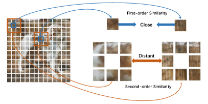
Figure 3. Illustration of First-order similarity and Second-order similarity.

However, the first-order similarity measure may not be sufficient to accurately capture complex inter-node relationships. As illustrated in Figure 3, the first-order similarity metric exhibits a bias towards low-level features such as color and texture, leading the model to select noisy neighbor nodes. In contrast, the second-order similarity is more semantic, as it describes the feature similarity of the central node’s neighbors in the Euclidean space. Second-order similarity can effectively compensate for the limitations of first-order similarity by rewarding connections between nodes that are similar to both themselves and their neighbors while penalizing the noisy nodes that are similar to themselves but dissimilar to their surroundings. This results in the model selecting more precise and semantically relevant node connections under sparse, limited connectivity.

To introduce the second-order similarity without additional computational cost, we propose a Progressively Separated Graph Construction called PSGC. As shown in Figure 2, the PSGC consists of two branches. The local branch has more channels to capture the contextual information of each node in the shallow layer. The other branch constructs the graph globally by computing the first-order similarity between nodes. Mathematically, we denote the input sequence of nodes as $x=\left({{x_{1}},\ldots,{x_{n}}}\right)$, and the output of the graph nodes $\tilde{x}=\left({{{\tilde{x}}_{1}},\ldots,{{\tilde{x}}_{n}}}\right)$, where ${x_{i}},{{\tilde{x}}_{i}}\in{R^{c}}$. The computation of our PVG block could be formulated as:

(7) $${{\tilde{x}}_{i}}=Concat\left[{f\left({{S_{ij}},x_{i}^{{h_{k}}},x_{j}^{{h_{k}}}}\right),\mathop{\sum}\limits_{j=1}^{n}{\alpha_{ij}}x_{j}^{C-{h_{k}}}}\right]$$

where $f$ is the nodes’ information aggregation and update function of the global graph. In addition, we set a distance threshold to the local branch, specifically set it to 0 if the Chebyshev distance of node $i$ and $j$ is greater than a threshold $r$($r$ defaults to 3).

As the model goes deeper, the proportion of local branch channels reduces, and the local branch gradually transfers a portion of its channels to the global graph. These channels have sufficiently absorbed local information in the shallow layers. Therefore, when the global graph computes the first-order similarity between nodes on these channels, it is equivalent to computing the second-order similarity between the nodes, which can be expressed as follows:

(8) $$S_{ij}^{2}=\mathop{\sum}\limits_{l}^{{h_{k+1}}-{h_{k}}}\left({\mathop{\sum}\limits_{t}^{{N_{i}}}{\alpha_{it}}x_{t}^{l}\cdot\mathop{\sum}\limits_{t}^{{N_{j}}}{\alpha_{jt}}x_{t}^{l}}\right)$$

where $h_{k}$ denotes the channels in the kth layer of the global graph and $x_{t}^{l}$ denotes the neighbor of node i or node j in the local branch.

PVG ultimately manifests as a trident structure, consisting of a local branch, a first-order similarity graph, and a second-order similarity graph. These three branches represent three distinct inductive biases in visual tasks: the local branch represents local dependency, the first-order similarity graph represents global dependency, and the second-order similarity graph represents a mixed dependency between local and global. The channel allocation ratio of the three branches can be controlled by adjusting the number of channels allocated to the progressive separation operation. However, we posit that all three structures at different levels are necessary, and the absence of any one of them would lead to a decrease in model capacity.

3.4. MaxE on node representation learning

After constructing the graph, it is necessary to design a nodes information update mechanism. Similar to CNNs, GNNs’ update process of node information at the l-th layer can be abstractly described as follows:

(9) $$x_{i}^{l+1}=\phi\left({x_{i}^{l},\rho\left({\{x_{j}^{l}|x_{j}^{l}\in{\rm N}\left({x_{i}^{l}}\right)\},x_{i}^{l},{W_{1}}}\right),{W_{2}}}\right)$$

where ${{\rm N}\left({x_{i}^{l}}\right)}$ represents the set of neighbors of node i at the l-th layer. $\rho$ is a node feature aggregation function and $\phi$ is a node feature update function. ${{W_{1}}}$ and ${{W_{2}}}$ are learnable matrices.

The difficulty of the node aggregation and update function $\phi$ lies in how to sample limited nodes from a given set of neighboring nodes to sufficiently represent the information of the entire set, as full sampling is expensive. We propose a concise yet comprehensive sampling strategy for the $\phi$, which is formulated as follows:

(10) $$x_{i}^{l+1}=W\cdot Concat\left[{x_{i}^{l},\max\left({x_{j}^{l}-x_{i}^{l}}\right),mean(x_{j}^{l})}\right]$$

It consists of three parts: self identity map, the maximum pooling of the difference between self and neighbor nodes, and the mathematical expectation of neighbor nodes. In other words, for a given set of neighboring nodes, the neighborhood information could be fully expressed by only sampling two points: the mean point and the point with the maximum difference from the central node.

To better understand the working mechanism of Formula 10, we need to have a detailed discussion on the key term $\rho$.

(11) $$\rho\left(\cdot\right)=\max\left({x_{j}^{l}-x_{i}^{l}|x_{j}^{l}\in{\rm N}\left({x_{i}^{l}}\right)}\right)$$

Another common form of $\rho$ in the field of GNN is as follows:

(12) $$\rho\left(\cdot\right)=\frac{1}{m}{\mathop{\sum}\limits_{j=1}^{m}\left({x_{j}^{l}-x_{i}^{l}|x_{j}^{l}\in{\rm N}\left({x_{i}^{l}}\right)}\right)}$$

Setting ${z_{1}}={x_{j}^{l}}-{x_{i}^{l}}$, then we define the following:

(13) $$z_{1}^{\prime}=\max\left({{z_{1}}}\right),{{\bar{z}}_{1}}=mean\left({{z_{1}}}\right)$$

(14) $$z_{1}^{\prime\prime}=\mathop{\arg\max}\limits_{{z_{1j}}}\left({z_{1}^{\prime}-{z_{1j}}}\right)$$

Then Formula 11 can be expressed as:

(15) $$\rho\left(\cdot\right) =\max\left({{z_{1}}}\right)$$

(16) $$={{\bar{z}}_{1}}+\left({z_{1}^{\prime}-{{\bar{z}}_{1}}}\right)$$

(17) $$={{\bar{z}}_{1}}+\left({z_{1}^{\prime\prime}-{{\bar{z}}_{1}}}\right)+\left({z_{1}^{\prime}-z_{1}^{\prime\prime}}\right)$$

(18) $$={{\bar{z}}_{1}}+\left({z_{1}^{\prime\prime}-{{\bar{z}}_{1}}}\right)+\max\left({z_{1}^{\prime}-{z_{1j}}}\right)$$

$\rho\left(\cdot\right)$ is divided into three parts: the first item is ${{\bar{z}}_{1}}$, which implies that Formula 12 is a subset of Formula 11; the second part is $\left({z_{1}^{\prime\prime}-{{\bar{z}}_{1}}}\right)$, which tends to be small so we call it the remainder; the third part is $\max\left({z_{1}^{\prime}-{z_{1j}}}\right)$, which we call the maximum bound within the class.

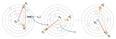
Figure 4. Illustration of neighbor sampling in MaxE.

We provide an illustration of the above ideas, as shown in Figure 4. In particular, if we let ${z_{2}}=z_{1}^{\prime}-{z_{1j}}$ for the third item above, there will be the following iterative form:

(19) $$\rho^{\prime}\left(\cdot\right) =\max\left(z_{1}^{\prime}-{{z_{1j}}}\right)$$

(20) $$={{\bar{z}}_{2}}+\left({z_{2}^{\prime\prime}-{{\bar{z}}_{2}}}\right)+\max\left({z_{2}^{\prime}-{z_{2j}}}\right)$$

If k times are iterated, there is the following k-order feature aggregation function $\rho$:

(21) $${\rho^{k-1}}\left(\cdot\right)={{\bar{z}}_{k}}+\left({z_{k}^{\prime\prime}-{{\bar{z}}_{k}}}\right)+\max\left(z_{k}^{\prime}-{{z_{kj}}}\right)$$

The final form of aggregate function $\rho$ can be expressed in the following abstract form:

(22) $$\rho\left(\cdot\right)=[{{\bar{z}}_{1}}+\cdots+{{\bar{z}}_{k}}]+\tilde{C}+{\rho^{k}}\left(\cdot\right)$$

where ${z_{1}}={x_{j}^{l}}-{x_{\scriptstyle i\hfill\atop\scriptstyle\hfill}^{l}}$, …, ${z_{2}}=z_{1}^{\prime}-{z_{1j}}$; ${\tilde{C}}$ is the accumulated remainder; ${\rho^{k}}\left(\cdot\right)$ is the k-order feature aggregation function.

Formula 22 is a form similar to the Taylor expansion, indicating that max pooling sampling iteratively retains the information of neighboring nodes at each order in an iterative manner. However, it still leaves out the zero-order neighbor information ${z_{0}}={x_{j}^{l}}-0$. For the completeness of information at each order, we add $mean(z_{0})$ in the final Formula 10. We refer to the final form as MaxE, it is a sufficiently rich sampling scheme for neighbor information. Adequate comparative experiments show that MaxE outperforms existing state-of-the-art graph representation learning methods for visual tasks.

3.5. GraphLU towards over-smoothing

In ViG (Han et al., 2022), over-smoothing phenomenon still appears in the deep layers. One intuitive solution is to add a non-linear transformation layer to enrich the node representation. However, this operation would increase computational overhead and model parameters. Therefore, we aimed to alleviate the over-smoothing problem with almost no increase in computation, and designed a new general activation function called Graph Linear Units (GraphLU).

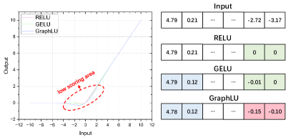
Figure 5. Illustration of GraphLU ($\varepsilon=1$) for alleviating the over-smoothing problem of graph network.

Firstly we review Relu (Hahnloser et al., 2000), from which we will derive the GraphLU. Relu is a zero-or-identity mapping, it performs an identity output for the high-value part of the input x, and zeros the low-value part:

(23) $$\operatorname{Re}LU\left(x\right)=\max\left({0,x}\right)$$

Our main idea is that the ReLU activation function discards some ”unimportant” parts of node representations, which results in a reduction of the node representation space and causes all outputs to converge to the same representation at deep layers. We think that these discarded ”unimportant” low-value information still contribute to the richness of the final node representations, as they often contain detailed information. Retaining some of these low-scoring information can significantly enrich the node representation. GELU (Hendrycks and Gimpel, 2016) is another activation function that retains some low-scoring information and has shown SOTA performance in Transformer models. We further discuss the potential of this relaxation operation by introducing a random variable $X_{ij}$.

(24) $${X_{ij}}\sim N\left({0,{{\left({1+\varepsilon}\right)}^{2}}}\right),{X_{ij}}\in{R^{m\times n}}$$

where m is the batch size , n is the number of nodes and $\varepsilon$ a learnable parameter. We hope that ${X_{ij}}$ with large values have a greater probability of being retained, but at the same time retain some ${X_{ij}}$ with small values hovering around 0. Assuming the input is ${x_{ij}}$, we can achieve this by defining the following probability:

(25) $$\phi\left({{x_{ij}}}\right)=p\left({{X_{ij}}\leq{x_{ij}}}\right)$$

That means, for an input ${x_{ij}}$, we describe the probability that the random variable ${X_{ij}}$ has a value less than its value, which can be found by integrating:

(26) $$\phi\left({{x_{ij}}}\right)=\mathop{\smallint}\nolimits_{-\infty}^{{x_{ij}}}\frac{1}{{\sqrt{2\pi}\left({1+\varepsilon}\right)}}{{\text{e}}^{-\frac{{{t^{2}}}}{{2{{\left({1+\varepsilon}\right)}^{2}}}}}}{\text{d}}t$$

An approximate expression is the Gauss Error function (erf), which is well supported in various deep learning frameworks, and the mathematical description is as follows:

(27) $$erf\left(\xi\right)=\frac{2}{{\sqrt{\pi}}}\mathop{\smallint}\nolimits_{0}^{\xi}{{\text{e}}^{-{t^{2}}}}{\text{dt}}$$

Let $t=\frac{z}{{\sqrt{2}(1+\varepsilon)}}$,then:

(28) $$erf\left(\xi\right)=\frac{2}{{\sqrt{2\pi}\left({1+\varepsilon}\right)}}[\mathop{\smallint}\nolimits_{-\infty}^{\sqrt{2}(1+\varepsilon)\xi}{{\text{e}}^{-\frac{{{z^{2}}}}{{2{{\left({1+\varepsilon}\right)}^{2}}}}}}{\text{dz - }}\phi\left(0\right)]$$

(29) $$2\phi\left({\sqrt{2}(1+\varepsilon)\xi}\right)=erf\left(\xi\right)+2\phi\left(0\right)$$

where $\phi\left(0\right)=\frac{1}{2}$, let $x=\sqrt{2}(1+\varepsilon)\xi$, we can get the final form of $\phi(x)$:

(30) $$\phi(x)=\frac{1}{2}erf\left[{\frac{x}{{\sqrt{2}(1+\varepsilon)}}+1}\right]$$

Multiply the input x by the probability $\phi(x)$ to get the final form of GraphLU:

(31) $$GraphLU(x)=0.5x\cdot erf\left[{\frac{x}{{\sqrt{2}(1+\varepsilon)}}+1}\right]$$

The above derivation follows the principle of GELU, but it reveals a key insight: by just adding a small relaxation perturbation $\varepsilon$ to the variance of the random variable $X_{ij}$, we can elegantly amplify detail information and enrich node features without introducing additional computational cost, thus alleviating over-smoothing issues.

4. Experiments

To demonstrate the effectiveness of PVG as a computer vision backbone, we conduct classification experiments on ImageNet1K (Deng et al., 2009), object detection experiments on COCO (Lin et al., 2014). In addition, we conduct comprehensive ablation experiments on the three main components in PVG to demonstrate that each part brings tangible improvements to the model. Furthermore, we provide some visualization experimental results to support our point of view.

4.1. Evaluation On IMAGENET-1K

For the fairness of the experiment,the input image size is 224x224,and we follow the training strategy in DeiT (Touvron et al., 2021), using the same data augmentations and regularization methods. Specifically, we use AdamW optimizer, and init learning rate $1\times{10^{-3}}$ with via cosine decaying. Furthermore, in order to support the generalization of downstream tasks and the stability of training, we use LePE (Dong et al., 2022) as the position embedding and use LayerScale (Zhu et al., 2021) in the last two layers.

We compare our PVG with those representative vision networks in Table 1, our PVG series can be comparable to the Transformer variants, and outperform the state-of-the-art CNN networks. In particular, compared with ViG (Han et al., 2022), which is also based on GNN, PVG has a significant lead in Top1-accuracy.

Table 1. Comparison of different models on ImageNet-1K.

Model	Mixing Type	Resolution	#Param.	FLOPs	Top-1
ResNet-50 (Wightman et al., 2021)	Conv	224$\times$224	26M	4.1G	79.8
ConvNeXt-T (Liu et al., 2022b)	Conv	224$\times$224	29M	4.5G	82.1
PVT-S (Wang et al., 2021)	Attn	224$\times$224	25M	3.8G	79.8
T2T-ViT-14 (Yuan et al., 2021)	Attn	224$\times$224	22M	4.8G	81.5
Swin-T (Liu et al., 2021a)	Attn	224$\times$224	29M	4.5G	81.3
ViL-S (Li et al., 2021a)	Attn	224$\times$224	25M	4.9G	81.8
Focal-T (Yang et al., 2021)	Attn	224$\times$224	29M	4.9G	82.2
CrossFormer-S (Wang et al., 2023)	Attn	224$\times$224	31M	4.9G	82.5
RegionViT-S (Chen et al., 2021a)	Attn	224$\times$224	31M	5.3G	82.6
ViG-S (Han et al., 2022)	Graph	224$\times$224	27M	4.6G	82.1
PVG-S(ours)	Graph	224$\times$224	22M	5.0G	83.0
ResNet-101 (Wightman et al., 2021)	Conv	224$\times$224	45M	7.9G	81.3
ConvNeXt-S (Liu et al., 2022b)	Conv	224$\times$224	50M	8.7G	83.1
PVT-M (Wang et al., 2021)	Attn	224$\times$224	44M	6.7G	81.2
T2T-ViT-19 (Yuan et al., 2021)	Attn	224$\times$224	39M	8.5G	81.9
Swin-S (Liu et al., 2021a)	Attn	224$\times$224	50M	8.7G	83.0
Focal-S (Yang et al., 2021)	Attn	224$\times$224	51M	9.1G	83.5
CrossFormer-B (Wang et al., 2023)	Attn	224$\times$224	52M	9.2G	83.4
RegionViT-M (Chen et al., 2021a)	Attn	224$\times$224	41M	7.4G	83.1
ViG-M (Han et al., 2022)	Graph	224$\times$224	52M	8.9G	83.1
PVG-M(ours)	Graph	224$\times$224	42M	8.9G	83.7
ResNet-152 (Wightman et al., 2021)	Conv	224$\times$224	60M	11.5G	81.8
ConvNeXt-B (Liu et al., 2022b)	Conv	224$\times$224	89M	15.4G	83.8
PVT-L (Wang et al., 2021)	Attn	224$\times$224	61M	9.8G	81.7
T2T-ViT-24 (Yuan et al., 2021)	Attn	224$\times$224	64M	13.8G	82.3
Swin-B (Liu et al., 2021a)	Attn	224$\times$224	88M	15.4G	83.5
ViL-B (Li et al., 2021a)	Attn	224$\times$224	56M	13.4G	83.2
Focal-B (Yang et al., 2021)	Attn	224$\times$224	90M	16.0G	83.8
CrossFormer-L (Wang et al., 2023)	Attn	224$\times$224	92M	16.6G	84.0
RegionViT-B (Chen et al., 2021a)	Attn	224$\times$224	73M	13.0G	83.2
ViG-B (Han et al., 2022)	Graph	224$\times$224	93M	16.8G	83.7
PVG-B(ours)	Graph	224$\times$224	79M	16.9G	84.2

(a) Input image

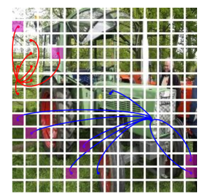
(b) ViG

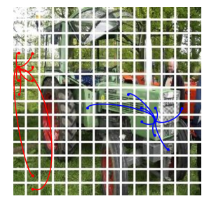
(c) PVG(ours)

Figure 6. Due to its monotonous first-order similarity measure, ViG finds some unreasonable neighbor nodes(the part marked in purple). Our PVG employs a hybrid similarity measure, which finds neighbors that are more accurate and focused.

To better understand how our PVG model works, we visualize the constructed graph structure in PVG-S and compare it with ViG-S. In Figure 6, we show a graph sample in the 12th blocks. Two center nodes are visualized as drawing all the edges will be messy. We can observe that ViG, lacking second-order similarity information, erroneously connects the grass node and the truck node (highlighted in purple) due to their similar green color. However, since our PVG employs a more complex hybrid similarity measure, it does not solely rely on low-level features such as color or texture to select neighboring nodes. Consequently, the neighbors of center nodes in PVG are more semantic and belong to the same category.

4.2. Evaluation On COCO

We conduct experiments on the COCO detection dataset to evaluate the generalization of PVG. We pretrain the backbones on the ImageNet-1K dataset and follow the finetuning used in Swin Transformer (Liu et al., 2021a) on the COCO dataset. The models are trained in the commonly-used “1x” schedule with 1280×800 input size.

Table 2. Object detection and instance segmentation results.

	MASK R-CNN 1$\times$ Schedule
	#Param(M)	FLOPs(G)	$A{P^{b}}$	$AP_{50}^{b}$	$AP_{75}^{b}$	$A{P^{m}}$	$AP_{50}^{m}$	$AP_{75}^{m}$
ResNet-50 (Wightman et al., 2021)	44.2	260.1	38.0	58.6	41.4	34.4	55.1	36.7
PVT-S (Wang et al., 2021)	44.1	245.1	40.4	62.9	43.8	37.8	60.1	40.3
Swin-T (Liu et al., 2021a)	47.8	264.0	42.2	64.6	46.2	39.1	61.6	42.2
CycleMLP-B2 (Chen et al., 2021b)	46.5	249.5	42.1	64.0	45.7	38.9	61.2	41.8
ViG-S (Han et al., 2022)	45.8	258.8	42.6	65.2	46.0	39.4	62.4	41.6
PVG-S(ours)	40.9	267.9	43.9	66.3	48.0	39.8	62.8	42.4

Table 2 compares our PVG with state-of-the-art GNN-based and Transformer-based architecture. The experimental results demonstrate that our PVG achieves further improvements in performance in object detection and can compete with other mainstream architectures. Additionally, Figure 7 visualizes some results of object detection and instance segmentation and achieves good detection and instance segmentation performance on sparse objects, dense objects, and moving objects.

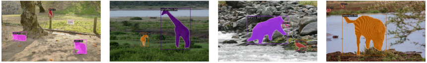
(a) Sparse objects

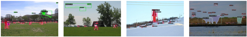
(b) Dense objects

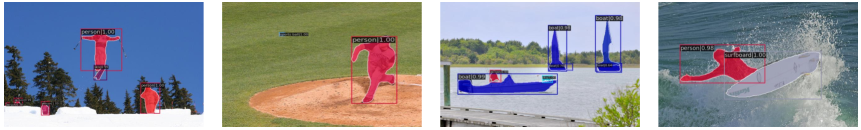
(c) Moving objects

Figure 7. Qualitative examples for object detection and instance segmentation on PVG-S+Mask R-CNN. Our PVG achieves good detection and instance segmentation performance on sparse objects, dense objects, and moving objects.

4.3. Ablation Study

In order to thoroughly examine the effectiveness of different PVG methods, we meticulously design a series of ablation experiments under a completely fair setting. Each experiment strictly adheres to the same architecture and hyperparameters, with only one component altered per ablation experiment. The comprehensive results of these ablation experiments are presented in Table 3. The findings clearly demonstrate the substantial impact of introducing second-order similarity information in the graph structure, as it significantly improves the overall performance. Additionally, our proposed novel graph node aggregation and update function, MaxE, as well as the newly designed activation function aimed at addressing over-smoothing, both contribute to further enhancing the model’s performance without introducing any additional computational cost.

Table 3. Ablation experiments of main methods in PVG.

Architecture design	Params(M)	FLOPs(G)	Top1(%)
Baseline (ViG-S layout)	27	4.6	81.9*
+PSGC for second-order similarity	22	4.9	82.5(+0.6)
MR GraphConv$\to$MaxE	22	4.9	82.8(+0.3)
GELU$\to$GraphLU	22	4.9	83.0(+0.2)

• denotes the reproduced result in our experimental settings.

In order to demonstrate the superiority of our designed nodes’ information update function MaxE, Table 4 conducts comparative experiments under the same settings. Compared with the two advanced methods in vision GNN, our MaxE has a best balance between accuracy and parameters, which achieve the accuracy improvements from 84.3 of MR GraphConv to 85.0. The benchmark unit of the parameters in the table is the parameters in GIN. (Due to limited computing resources, the data is a randomly selected subset of Imagenet, with a training set of 60,000 images and 150 categories.)

Table 4. Comparison of MaxE with other aggregate functions.

	GIN	MR GraphConv	EdgeConv	GraphSAGE	MaxE(ours)
Top1-acc	80.55	84.3	85.0	83.76	85.0
Params	1	2	10	11	3

4.4. Over-smoothing analysis

Figure 8. GraphLU alleviates the over-smoothing phenomenon in the deep layer without increasing the computational cost.

We use Imagenet-1K to train two small PVG models with 21 layers under the exact same setting. The only difference between them is that one uses GELU as the activation function, and the other uses our GraphLU. As shown in Figure 8, the node features distinctiveness of PVG using GELU drops sharply from layer 17 to layer 21 until the last layer is almost 0, where $diversity=\frac{1}{n}\sum\limits_{i=1}^{n}\left\|{x_{i}-\frac{1}{n}\sum\limits_{i=1}^{n}x_{i}}\right\|_{2}$. However, the over-smoothing phenomenon of PVG with GraphLU has been alleviated. The node features distinctiveness only decreases once, and stay at an acceptable level in the last few layers instead of dropping to 0. Notably, GraphLU achieves a certain level of alleviation of the over-smoothing issue, albeit not as pronounced as in some other methods. Importantly, this improvement is attained with minimal computational overhead. Furthermore, it outperforms any previous endeavors dedicated to tackling the over-smoothing problem, exhibiting notably higher training efficiency.

5. Conclusion

In this work, we explore graph-based backbone network design for vision and introduce a novel structure named Progressive Vision Graph (PVG). PVG constructs two separate graphs for global and local modeling and a fast graph node aggregation and update mechanism MaxE for neighbor nodes. In addition, we propose a concise activation function to effectively solve the over-smoothing phenomenon in previous work, which allows the vision GNN network to be stacked to 20 layers or even deeper to deal with various complex vision tasks. Extensive experiments on image recognition and object detection demonstrate the superiority of the proposed PVG architecture compared with previous state-of-the-art works. In summary, our proposed PVG accelerates the generalization process of graph neural networks towards computer vision tasks. This advancement positions GNN as a compelling contender for the unified architecture of image, language, and graph-structured data in the future.

References

- (1)
- Abu-El-Haija et al. (2019) Sami Abu-El-Haija, Bryan Perozzi, Amol Kapoor, Nazanin Alipourfard, Kristina Lerman, Hrayr Harutyunyan, Greg Ver Steeg, and Aram Galstyan. 2019. Mixhop: Higher-order graph convolutional architectures via sparsified neighborhood mixing. In international conference on machine learning. PMLR, 21–29.
- Atwood and Towsley (2016) James Atwood and Don Towsley. 2016. Diffusion-convolutional neural networks. Advances in neural information processing systems 29 (2016).
- Bruna et al. (2013) Joan Bruna, Wojciech Zaremba, Arthur Szlam, and Yann LeCun. 2013. Spectral networks and locally connected networks on graphs. arXiv preprint arXiv:1312.6203 (2013).
- Chen et al. (2022) Chaoqi Chen, Jiongcheng Li, Xiaoguang Han, Xiaoqing Liu, and Yizhou Yu. 2022. Compound domain generalization via meta-knowledge encoding. In Proceedings of the IEEE/CVF Conference on Computer Vision and Pattern Recognition. 7119–7129.
- Chen et al. (2021a) Chun-Fu Chen, Rameswar Panda, and Quanfu Fan. 2021a. Regionvit: Regional-to-local attention for vision transformers. arXiv preprint arXiv:2106.02689 (2021).
- Chen et al. (2021b) Shoufa Chen, Enze Xie, Chongjian Ge, Runjian Chen, Ding Liang, and Ping Luo. 2021b. Cyclemlp: A mlp-like architecture for dense prediction. arXiv preprint arXiv:2107.10224 (2021).
- Chen et al. (2020) Yu Chen, Lingfei Wu, and Mohammed Zaki. 2020. Iterative deep graph learning for graph neural networks: Better and robust node embeddings. Advances in neural information processing systems 33 (2020), 19314–19326.
- Chen et al. (2019b) Yu Chen, Lingfei Wu, and Mohammed J Zaki. 2019b. Graphflow: Exploiting conversation flow with graph neural networks for conversational machine comprehension. arXiv preprint arXiv:1908.00059 (2019).
- Chen et al. (2019c) Yu Chen, Lingfei Wu, and Mohammed J Zaki. 2019c. Reinforcement learning based graph-to-sequence model for natural question generation. arXiv preprint arXiv:1908.04942 (2019).
- Chen et al. (2019a) Zhao-Min Chen, Xiu-Shen Wei, Peng Wang, and Yanwen Guo. 2019a. Multi-label image recognition with graph convolutional networks. In Proceedings of the IEEE/CVF conference on computer vision and pattern recognition. 5177–5186.
- Dai et al. (2021) Zihang Dai, Hanxiao Liu, Quoc V Le, and Mingxing Tan. 2021. Coatnet: Marrying convolution and attention for all data sizes. Advances in Neural Information Processing Systems 34 (2021), 3965–3977.
- Defferrard et al. (2016) Michaël Defferrard, Xavier Bresson, and Pierre Vandergheynst. 2016. Convolutional neural networks on graphs with fast localized spectral filtering. Advances in neural information processing systems 29 (2016).
- Deng et al. (2009) Jia Deng, Wei Dong, Richard Socher, Li-Jia Li, Kai Li, and Li Fei-Fei. 2009. Imagenet: A large-scale hierarchical image database. In 2009 IEEE conference on computer vision and pattern recognition. Ieee, 248–255.
- Ding et al. (2022) Xiaohan Ding, Xiangyu Zhang, Jungong Han, and Guiguang Ding. 2022. Scaling up your kernels to 31x31: Revisiting large kernel design in cnns. In Proceedings of the IEEE/CVF Conference on Computer Vision and Pattern Recognition. 11963–11975.
- Dong et al. (2022) Xiaoyi Dong, Jianmin Bao, Dongdong Chen, Weiming Zhang, Nenghai Yu, Lu Yuan, Dong Chen, and Baining Guo. 2022. Cswin transformer: A general vision transformer backbone with cross-shaped windows. In Proceedings of the IEEE/CVF Conference on Computer Vision and Pattern Recognition. 12124–12134.
- Dosovitskiy et al. (2020) Alexey Dosovitskiy, Lucas Beyer, Alexander Kolesnikov, Dirk Weissenborn, Xiaohua Zhai, Thomas Unterthiner, Mostafa Dehghani, Matthias Minderer, Georg Heigold, Sylvain Gelly, et al. 2020. An image is worth 16x16 words: Transformers for image recognition at scale. arXiv preprint arXiv:2010.11929 (2020).
- Gao et al. (2021) Peng Gao, Jiasen Lu, Hongsheng Li, Roozbeh Mottaghi, and Aniruddha Kembhavi. 2021. Container: Context aggregation network. arXiv preprint arXiv:2106.01401 (2021).
- Gasteiger et al. (2019) Johannes Gasteiger, Stefan Weißenberger, and Stephan Günnemann. 2019. Diffusion improves graph learning. Advances in neural information processing systems 32 (2019).
- Hahnloser et al. (2000) Richard HR Hahnloser, Rahul Sarpeshkar, Misha A Mahowald, Rodney J Douglas, and H Sebastian Seung. 2000. Digital selection and analogue amplification coexist in a cortex-inspired silicon circuit. nature 405, 6789 (2000), 947–951.
- Hamilton et al. (2017) Will Hamilton, Zhitao Ying, and Jure Leskovec. 2017. Inductive representation learning on large graphs. Advances in neural information processing systems 30 (2017).
- Han et al. (2022) Kai Han, Yunhe Wang, Jianyuan Guo, Yehui Tang, and Enhua Wu. 2022. Vision gnn: An image is worth graph of nodes. arXiv preprint arXiv:2206.00272 (2022).
- Han et al. (2023) Yue Han, Jiangning Zhang, Zhucun Xue, Chao Xu, Xintian Shen, Yabiao Wang, Chengjie Wang, Yong Liu, and Xiangtai Li. 2023. Reference Twice: A Simple and Unified Baseline for Few-Shot Instance Segmentation. arXiv preprint arXiv:2301.01156 (2023).
- He et al. (2016) Kaiming He, Xiangyu Zhang, Shaoqing Ren, and Jian Sun. 2016. Deep residual learning for image recognition. In Proceedings of the IEEE conference on computer vision and pattern recognition. 770–778.
- Henaff et al. (2015) Mikael Henaff, Joan Bruna, and Yann LeCun. 2015. Deep convolutional networks on graph-structured data. arXiv preprint arXiv:1506.05163 (2015).
- Hendrycks and Gimpel (2016) Dan Hendrycks and Kevin Gimpel. 2016. Bridging nonlinearities and stochastic regularizers with gaussian error linear units. CoRR, abs/1606.08415 3 (2016).
- Howard et al. (2017) Andrew G Howard, Menglong Zhu, Bo Chen, Dmitry Kalenichenko, Weijun Wang, Tobias Weyand, Marco Andreetto, and Hartwig Adam. 2017. Mobilenets: Efficient convolutional neural networks for mobile vision applications. arXiv preprint arXiv:1704.04861 (2017).
- Hu et al. (2020) Hanzhe Hu, Deyi Ji, Weihao Gan, Shuai Bai, Wei Wu, and Junjie Yan. 2020. Class-wise dynamic graph convolution for semantic segmentation. In Computer Vision–ECCV 2020: 16th European Conference, Glasgow, UK, August 23–28, 2020, Proceedings, Part XVII 16. Springer, 1–17.
- Huang et al. (2018) Wenbing Huang, Tong Zhang, Yu Rong, and Junzhou Huang. 2018. Adaptive sampling towards fast graph representation learning. Advances in neural information processing systems 31 (2018).
- Kampffmeyer et al. (2019) Michael Kampffmeyer, Yinbo Chen, Xiaodan Liang, Hao Wang, Yujia Zhang, and Eric P Xing. 2019. Rethinking knowledge graph propagation for zero-shot learning. In Proceedings of the IEEE/CVF conference on computer vision and pattern recognition. 11487–11496.
- Kipf and Welling (2016) Thomas N Kipf and Max Welling. 2016. Semi-supervised classification with graph convolutional networks. arXiv preprint arXiv:1609.02907 (2016).
- Krizhevsky et al. (2017) Alex Krizhevsky, Ilya Sutskever, and Geoffrey E Hinton. 2017. Imagenet classification with deep convolutional neural networks. Commun. ACM 60, 6 (2017), 84–90.
- LeCun et al. (1998) Yann LeCun, Léon Bottou, Yoshua Bengio, and Patrick Haffner. 1998. Gradient-based learning applied to document recognition. Proc. IEEE 86, 11 (1998), 2278–2324.
- Levie et al. (2018) Ron Levie, Federico Monti, Xavier Bresson, and Michael M Bronstein. 2018. Cayleynets: Graph convolutional neural networks with complex rational spectral filters. IEEE Transactions on Signal Processing 67, 1 (2018), 97–109.
- Li et al. (2019a) Guohao Li, Matthias Muller, Ali Thabet, and Bernard Ghanem. 2019a. Deepgcns: Can gcns go as deep as cnns?. In Proceedings of the IEEE/CVF international conference on computer vision. 9267–9276.
- Li et al. (2019b) Jian Li, Yabiao Wang, Changan Wang, Ying Tai, Jianjun Qian, Jian Yang, Chengjie Wang, Jilin Li, and Feiyue Huang. 2019b. DSFD: dual shot face detector. In Proceedings of the IEEE/CVF Conference on Computer Vision and Pattern Recognition. 5060–5069.
- Li et al. (2021b) Jian Li, Bin Zhang, Yabiao Wang, Ying Tai, Zhenyu Zhang, Chengjie Wang, Jilin Li, Xiaoming Huang, and Yili Xia. 2021b. ASFD: Automatic and scalable face detector. In Proceedings of the 29th ACM International Conference on Multimedia. 2139–2147.
- Li et al. (2022b) Kunchang Li, Yali Wang, Peng Gao, Guanglu Song, Yu Liu, Hongsheng Li, and Yu Qiao. 2022b. Uniformer: Unified transformer for efficient spatiotemporal representation learning. arXiv preprint arXiv:2201.04676 (2022).
- Li et al. (2018a) Qimai Li, Zhichao Han, and Xiao-Ming Wu. 2018a. Deeper insights into graph convolutional networks for semi-supervised learning. In Proceedings of the AAAI conference on artificial intelligence, Vol. 32.
- Li et al. (2018b) Ruoyu Li, Sheng Wang, Feiyun Zhu, and Junzhou Huang. 2018b. Adaptive graph convolutional neural networks. In Proceedings of the AAAI conference on artificial intelligence, Vol. 32.
- Li et al. (2022a) Wuyang Li, Xinyu Liu, and Yixuan Yuan. 2022a. Sigma: Semantic-complete graph matching for domain adaptive object detection. In Proceedings of the IEEE/CVF Conference on Computer Vision and Pattern Recognition. 5291–5300.
- Li et al. (2022c) Xiangtai Li, Jiangning Zhang, Yibo Yang, Guangliang Cheng, Kuiyuan Yang, Yu Tong, and Dacheng Tao. 2022c. SFNet: Faster, Accurate, and Domain Agnostic Semantic Segmentation via Semantic Flow. ArXiv abs/2207.04415 (2022).
- Li et al. (2021a) Yawei Li, Kai Zhang, Jiezhang Cao, Radu Timofte, and Luc Van Gool. 2021a. Localvit: Bringing locality to vision transformers. arXiv preprint arXiv:2104.05707 (2021).
- Lin et al. (2014) Tsung-Yi Lin, Michael Maire, Serge Belongie, James Hays, Pietro Perona, Deva Ramanan, Piotr Dollár, and C Lawrence Zitnick. 2014. Microsoft coco: Common objects in context. In Computer Vision–ECCV 2014: 13th European Conference, Zurich, Switzerland, September 6-12, 2014, Proceedings, Part V 13. Springer, 740–755.
- Liu et al. (2021b) Lu Liu, Tianyi Zhou, Guodong Long, Jing Jiang, Xuanyi Dong, and Chengqi Zhang. 2021b. Isometric propagation network for generalized zero-shot learning. arXiv preprint arXiv:2102.02038 (2021).
- Liu et al. (2022a) Ze Liu, Han Hu, Yutong Lin, Zhuliang Yao, Zhenda Xie, Yixuan Wei, Jia Ning, Yue Cao, Zheng Zhang, Li Dong, et al. 2022a. Swin transformer v2: Scaling up capacity and resolution. In Proceedings of the IEEE/CVF conference on computer vision and pattern recognition. 12009–12019.
- Liu et al. (2021a) Ze Liu, Yutong Lin, Yue Cao, Han Hu, Yixuan Wei, Zheng Zhang, Stephen Lin, and Baining Guo. 2021a. Swin transformer: Hierarchical vision transformer using shifted windows. In Proceedings of the IEEE/CVF international conference on computer vision. 10012–10022.
- Liu et al. (2022b) Zhuang Liu, Hanzi Mao, Chao-Yuan Wu, Christoph Feichtenhofer, Trevor Darrell, and Saining Xie. 2022b. A convnet for the 2020s. In Proceedings of the IEEE/CVF Conference on Computer Vision and Pattern Recognition. 11976–11986.
- Luo et al. (2020) Yadan Luo, Zijian Wang, Zi Huang, and Mahsa Baktashmotlagh. 2020. Progressive graph learning for open-set domain adaptation. In International Conference on Machine Learning. PMLR, 6468–6478.
- Ma et al. (2019) Xinhong Ma, Tianzhu Zhang, and Changsheng Xu. 2019. Gcan: Graph convolutional adversarial network for unsupervised domain adaptation. In Proceedings of the IEEE/CVF Conference on Computer Vision and Pattern Recognition. 8266–8276.
- Monti et al. (2017) Federico Monti, Davide Boscaini, Jonathan Masci, Emanuele Rodola, Jan Svoboda, and Michael M Bronstein. 2017. Geometric deep learning on graphs and manifolds using mixture model cnns. In Proceedings of the IEEE conference on computer vision and pattern recognition. 5115–5124.
- Niepert et al. (2016) Mathias Niepert, Mohamed Ahmed, and Konstantin Kutzkov. 2016. Learning convolutional neural networks for graphs. In International conference on machine learning. PMLR, 2014–2023.
- Rong et al. (2019) Yu Rong, Wenbing Huang, Tingyang Xu, and Junzhou Huang. 2019. Dropedge: Towards deep graph convolutional networks on node classification. arXiv preprint arXiv:1907.10903 (2019).
- Roy et al. (2021) Subhankar Roy, Evgeny Krivosheev, Zhun Zhong, Nicu Sebe, and Elisa Ricci. 2021. Curriculum graph co-teaching for multi-target domain adaptation. In Proceedings of the IEEE/CVF Conference on Computer Vision and Pattern Recognition. 5351–5360.
- Simonyan and Zisserman (2014) Karen Simonyan and Andrew Zisserman. 2014. Very deep convolutional networks for large-scale image recognition. arXiv preprint arXiv:1409.1556 (2014).
- Szegedy et al. (2015) Christian Szegedy, Wei Liu, Yangqing Jia, Pierre Sermanet, Scott Reed, Dragomir Anguelov, Dumitru Erhan, Vincent Vanhoucke, and Andrew Rabinovich. 2015. Going deeper with convolutions. In Proceedings of the IEEE conference on computer vision and pattern recognition. 1–9.
- Touvron et al. (2021) Hugo Touvron, Matthieu Cord, Matthijs Douze, Francisco Massa, Alexandre Sablayrolles, and Hervé Jégou. 2021. Training data-efficient image transformers & distillation through attention. In International conference on machine learning. PMLR, 10347–10357.
- Veličković et al. (2017) Petar Veličković, Guillem Cucurull, Arantxa Casanova, Adriana Romero, Pietro Lio, and Yoshua Bengio. 2017. Graph attention networks. arXiv preprint arXiv:1710.10903 (2017).
- Wang et al. (2016) Daixin Wang, Peng Cui, and Wenwu Zhu. 2016. Structural deep network embedding. In Proceedings of the 22nd ACM SIGKDD international conference on Knowledge discovery and data mining. 1225–1234.
- Wang et al. (2020) Tianming Wang, Xiaojun Wan, and Hanqi Jin. 2020. Amr-to-text generation with graph transformer. Transactions of the Association for Computational Linguistics 8 (2020), 19–33.
- Wang et al. (2023) Wenxiao Wang, Wei Chen, Qibo Qiu, Long Chen, Boxi Wu, Binbin Lin, Xiaofei He, and Wei Liu. 2023. CrossFormer++: A Versatile Vision Transformer Hinging on Cross-scale Attention. arXiv preprint arXiv:2303.06908 (2023).
- Wang et al. (2021) Wenhai Wang, Enze Xie, Xiang Li, Deng-Ping Fan, Kaitao Song, Ding Liang, Tong Lu, Ping Luo, and Ling Shao. 2021. Pyramid vision transformer: A versatile backbone for dense prediction without convolutions. In Proceedings of the IEEE/CVF international conference on computer vision. 568–578.
- Wang et al. (2019) Yue Wang, Yongbin Sun, Ziwei Liu, Sanjay E Sarma, Michael M Bronstein, and Justin M Solomon. 2019. Dynamic graph cnn for learning on point clouds. Acm Transactions On Graphics (tog) 38, 5 (2019), 1–12.
- Wightman et al. (2021) Ross Wightman, Hugo Touvron, and Hervé Jégou. 2021. Resnet strikes back: An improved training procedure in timm. arXiv preprint arXiv:2110.00476 (2021).
- Wu et al. (2021) Haiping Wu, Bin Xiao, Noel Codella, Mengchen Liu, Xiyang Dai, Lu Yuan, and Lei Zhang. 2021. Cvt: Introducing convolutions to vision transformers. In Proceedings of the IEEE/CVF International Conference on Computer Vision. 22–31.
- Wu et al. (2023) Jianzong Wu, Xiangtai Li, Shilin Xu Haobo Yuan, Henghui Ding, Yibo Yang, Xia Li, Jiangning Zhang, Yunhai Tong, Xudong Jiang, Bernard Ghanem, et al. 2023. Towards Open Vocabulary Learning: A Survey. arXiv preprint arXiv:2306.15880 (2023).
- Wu et al. (2020) Yangxin Wu, Gengwei Zhang, Yiming Gao, Xiajun Deng, Ke Gong, Xiaodan Liang, and Liang Lin. 2020. Bidirectional graph reasoning network for panoptic segmentation. In Proceedings of the IEEE/CVF Conference on Computer Vision and Pattern Recognition. 9080–9089.
- Xu et al. (2018) Keyulu Xu, Chengtao Li, Yonglong Tian, Tomohiro Sonobe, Ken-ichi Kawarabayashi, and Stefanie Jegelka. 2018. Representation learning on graphs with jumping knowledge networks. In International conference on machine learning. PMLR, 5453–5462.
- Xu et al. (2021) Yufei Xu, Qiming Zhang, Jing Zhang, and Dacheng Tao. 2021. Vitae: Vision transformer advanced by exploring intrinsic inductive bias. Advances in Neural Information Processing Systems 34 (2021), 28522–28535.
- Yang et al. (2021) Jianwei Yang, Chunyuan Li, Pengchuan Zhang, Xiyang Dai, Bin Xiao, Lu Yuan, and Jianfeng Gao. 2021. Focal self-attention for local-global interactions in vision transformers. arXiv preprint arXiv:2107.00641 (2021).
- Yang et al. (2020) Ling Yang, Liangliang Li, Zilun Zhang, Xinyu Zhou, Erjin Zhou, and Yu Liu. 2020. Dpgn: Distribution propagation graph network for few-shot learning. In Proceedings of the IEEE/CVF conference on computer vision and pattern recognition. 13390–13399.
- You et al. (2020) Renchun You, Zhiyao Guo, Lei Cui, Xiang Long, Yingze Bao, and Shilei Wen. 2020. Cross-modality attention with semantic graph embedding for multi-label classification. In Proceedings of the AAAI conference on artificial intelligence, Vol. 34. 12709–12716.
- Yuan et al. (2021) Li Yuan, Yunpeng Chen, Tao Wang, Weihao Yu, Yujun Shi, Zi-Hang Jiang, Francis EH Tay, Jiashi Feng, and Shuicheng Yan. 2021. Tokens-to-token vit: Training vision transformers from scratch on imagenet. In Proceedings of the IEEE/CVF international conference on computer vision. 558–567.
- Zhang et al. (2023) Jiangning Zhang, Xiangtai Li, Jian Li, Liang Liu, Zhucun Xue, Boshen Zhang, Zhengkai Jiang, Tianxin Huang, Yabiao Wang, and Chengjie Wang. 2023. Rethinking Mobile Block for Efficient Neural Models. ICCV (2023).
- Zhang et al. (2022) Jiangning Zhang, Xiangtai Li, Yabiao Wang, Chengjie Wang, Yibo Yang, Yong Liu, and Dacheng Tao. 2022. Eatformer: Improving vision transformer inspired by evolutionary algorithm. arXiv preprint arXiv:2206.09325 (2022).
- Zhang et al. (2021) Jiangning Zhang, Chao Xu, Jian Li, Wenzhou Chen, Yabiao Wang, Ying Tai, Shuo Chen, Chengjie Wang, Feiyue Huang, and Yong Liu. 2021. Analogous to evolutionary algorithm: Designing a unified sequence model. NeurIPS 34 (2021), 26674–26688.
- Zhang et al. (2020) Li Zhang, Dan Xu, Anurag Arnab, and Philip HS Torr. 2020. Dynamic graph message passing networks. In Proceedings of the IEEE/CVF Conference on Computer Vision and Pattern Recognition. 3726–3735.
- Zhao et al. (2021) Gangming Zhao, Weifeng Ge, and Yizhou Yu. 2021. GraphFPN: Graph feature pyramid network for object detection. In Proceedings of the IEEE/CVF international conference on computer vision. 2763–2772.
- Zhao and Akoglu (2019) Lingxiao Zhao and Leman Akoglu. 2019. Pairnorm: Tackling oversmoothing in gnns. arXiv preprint arXiv:1909.12223 (2019).
- Zhu et al. (2021) Chen Zhu, Renkun Ni, Zheng Xu, Kezhi Kong, W Ronny Huang, and Tom Goldstein. 2021. Gradinit: Learning to initialize neural networks for stable and efficient training. Advances in Neural Information Processing Systems 34 (2021), 16410–16422.
- Zhu and Koniusz (2021) Hao Zhu and Piotr Koniusz. 2021. Simple spectral graph convolution. In International conference on learning representations.