\jvol

XX \jnumXX \jmonthXXXXX \paper1234567 \doiinfoTAES.2020.Doi Number

\member

Member, IEEE

\authoraddress

Z. Guo, X. Gu, Y. Han, and J. Guo are with the Institute of Precision Guidance, and Control, Northwestern Polytechnical University, Xi’an 710072, China, (e-mail: guozongyi@nwpu.edu.cn; guxiyu@mail.nwpu.edu.cn; hanyonglin@mail.nwpu.edu.cn; guojianguo@nwpu.edu.cn). T. Berger is with the Universität Paderborn, Institut für Mathematik, Warburger Str. 100, 33098 Paderborn, Germany, (thomas.berger@math.upb.de). (Corresponding author: Zongyi Guo.)

\editor

This work was supported by the National Natural Science Foundation of China under Grant 92271109 and Grant 52272404 and the Deutsche Forschungsgemeinschaft (DFG, German Research Foundation) under Project-IDs 362536361 and 471539468.

Maneuvering tracking algorithm for reentry vehicles with guaranteed prescribed performance

ZONGYI GUO    XIYU GU    YONGLIN HAN    JIANGUO GUO Northwestern Polytechnical University Xi’an, China    THOMAS BERGER Institut für Mathematik, Universität Paderborn, Germany
(2020)
Abstract

This paper presents a prescribed performance-based tracking control strategy for the atmospheric reentry flight of space vehicles subject to rapid maneuvers during flight mission. A time-triggered non-monotonic performance funnel is proposed with the aim of constraints violation avoidance in the case of sudden changes of the reference trajectory. Compared with traditional prescribed performance control methods, the novel funnel boundary is adaptive with respect to the reference path and is capable of achieving stability under disturbances. A recursive control structure is introduced which does not require any knowledge of specific system parameters. By a stability analysis we show that the tracking error evolves within the prescribed error margin under a condition which represents a trade-off between the reference signal and the performance funnel. The effectiveness of the proposed control scheme is verified by simulations.

Index Terms–Reentry vehicles, tracking with prescribed performance, funnel control, maneuvering trajectory tracking

1 INTRODUCTION

For the cost efficiency of space missions it is imperative that spacecrafts are able to return to earth through its atmosphere, following a prescribed trajectory. Such atmospheric reentry problems are a main focus of the aerospace industry and have received a large amount of attention during the last decade. Trajectory tracking strategies for reentry vehicles (RVs), characterized by high flight velocity, short response time and large envelope advantages, have long been considered as a hot research area due to its extensive applications in engineering [1]-[4]. Maneuvering flight has stimulated extensive research in the areas of evasion, pursuit and obstacle avoidance for missions achievement [5]-[8]. Commonly, the main objective of maneuvering flight control is stability and robustness of the system and to provide the stabilization capabilities in RV tracking either on-line or for off-line planned reference trajectories. Some widespread control approaches, including PID [9], sliding mode control [10], backstepping control [11], adaptive control [12]-[13] and intelligent algorithms [14]-[15], are the popular choice owing to their simplicity and effectiveness in RV tracking problems. However, apart from the steady state characteristics, also the transient behavior must be taken into account for a successful mission. As RVs travel at very high velocities, the aforementioned control methods, which only focus on the steady state behavior, are not applicable in this context. Although those results demonstrated that the tracking objective can be successfully accomplished, it remains an open issue how to guarantee its high speed convergence, minimum accuracy and small overshoot.

To resolve these drawbacks, control algorithms for constraining the transient performance are flourishing during the past few decades, and two different approaches have been developed. Prescribed performance control (PPC) has been proposed in [16]-[18] and is regarded as a representative nowadays. It relies on an error transformation, which is designed to transform the original output error restrictions into an equivalent interval one. Since its universal control structure, PPC has been thoroughly investigated in combination with unconstrained control methods like backstepping and sliding mode control. Funnel control (FC) is the second control mechanism for guaranteeing a prescribed performance of the tracking error [19]-[23] by introducing a time-varying high-gain feedback in the control law. If the error tends towards the funnel boundary, the gain increases so that the error is kept inside the performance funnel. Both PPC and FC have already been investigated for the control algorithm design for RVs with a focus on the transient performance [24]-[26]. Notice that almost all funnel boundaries selected in works on funnel control are monotonically decreasing functions, although the theory guarantees the stability of the closed-loop system for a vast variety of non-monotonic funnel boundaries. It turns out that for flight maneuvering, non-monotonic funnel boundaries are more suitable. Sudden flight maneuvers may lead to a drastic increase of the control effort or even drive the tracking error across the funnel boundary, resulting in closed-loop system instability.

Considering the various demands of trajectory tracking for RVs during different phases, a control law which adapts itself to the prescribed boundary function is required to guarantee the transient behavior in flight maneuvering. Therefore, a time triggered non-monotonic funnel boundary is proposed in this paper. Using a priori information of the reference trajectory, we design a boundary function which is widened during critical phases, e.g. in the case of sudden course corrections. In this way, peaks in the control input signal are avoided. Additionally, disturbances (such as noises, uncertainties or unmodeled dynamics) are taken into account, as they might have a detrimental effect on the system’s performance. A significant challenge in stability analysis is imposed by the dynamics of the RV, where the flight altitude (which is the system output) is influenced by the deflection angle only in a saturated way (via a sin\sin function). Therefore, arbitrary instantaneous changes of the altitude are not possible. Any prescribed trajectory can only be tracked up to a certain accuracy, i.e., there is a trade-off between the derivative of the reference and the funnel boundary function. To the best of our knowledge, this is the first work where such a trade-off is found for RV tracking problems with guaranteed prescribed performance.

Focusing on the issues mentioned above, the main contributions of this paper are summarized as follows.

  • A recursive funnel control structure with low complexity is adopted to avoid the requirement of a priori knowledge of system parameters.

  • We design a robust funnel control law with time triggered non-monotonic funnel boundary for flight maneuvering with guaranteed transient performance under disturbances.

  • We derive a condition representing a trade-off between the reference trajectory and the funnel boundaries, under which the RV is amenable to the proposed funnel control law.

The remainder of this paper is organized as follows. The dynamic model of the RV in yaw channel is presented in Section 2, together with the proposed funnel boundary and the control objective. In Section 3 we state the funnel-based control law design and provide the stability analysis. Simulation results are given in Section 4 and Section 5 finally concludes this article.

2 PROBLEM FORMULATION

2.1 RV Dynamics

Considering horizontal lateral maneuvers with constant velocity, the simplified model of a RV in yaw channel is established in [27, 28] and is of the form

z˙h(t)subscript˙𝑧𝑡\displaystyle{{\dot{z}}_{h}}\left(t\right) =Vsin(ψV(t))+Δ0(t)absent𝑉subscript𝜓𝑉𝑡subscriptΔ0𝑡\displaystyle=-V\sin\left({{\psi_{V}}\left(t\right)}\right)+\Delta_{0}(t) (1)
ψ˙V(t)subscript˙𝜓𝑉𝑡\displaystyle{{\dot{\psi}}_{V}}\left(t\right) =1mVZ(t)+Δ1(t)absent1𝑚𝑉𝑍𝑡subscriptΔ1𝑡\displaystyle=-\frac{1}{{mV}}Z\left(t\right)+\Delta_{1}(t) (2)
ψ˙(t)˙𝜓𝑡\displaystyle\dot{\psi}\left(t\right) =ωy(t)+Δ2(t)absentsubscript𝜔𝑦𝑡subscriptΔ2𝑡\displaystyle={\omega_{y}}\left(t\right)+\Delta_{2}(t) (3)
ω˙y(t)subscript˙𝜔𝑦𝑡\displaystyle{{\dot{\omega}}_{y}}\left(t\right) =My(t)Jy+Δ3(t)absentsubscript𝑀𝑦𝑡subscript𝐽𝑦subscriptΔ3𝑡\displaystyle=\frac{{{M_{y}}\left(t\right)}}{{{J_{y}}}}+\Delta_{3}(t) (4)
β(t)𝛽𝑡\displaystyle\beta\left(t\right) =ψ(t)ψV(t)absent𝜓𝑡subscript𝜓𝑉𝑡\displaystyle=\psi\left(t\right)-{\psi_{V}}\left(t\right) (5)

where zhsubscript𝑧z_{h} is the flight altitude, m𝑚m is the mass, V𝑉V is the flight speed, ψVsubscript𝜓𝑉\psi_{V}, ψ𝜓\psi, β𝛽\beta represent the deflection angle, yaw angle and sideslip angle, ωysubscript𝜔𝑦\omega_{y} is the yaw rate, Jysubscript𝐽𝑦J_{y} denotes the yaw rotational inertia and ΔisubscriptΔ𝑖\Delta_{i} (i=0,1,2,3)𝑖0123(i=0,1,2,3) are bounded disturbances. The functions Z𝑍Z and Mysubscript𝑀𝑦M_{y} are the aerodynamic force and moment in yaw channel, expressed by Z(t)=q¯S(czαα+czββ(t)+cz0)𝑍𝑡¯𝑞𝑆superscriptsubscript𝑐𝑧𝛼𝛼superscriptsubscript𝑐𝑧𝛽𝛽𝑡superscriptsubscript𝑐𝑧0Z(t)=\bar{q}S({c_{z}^{\alpha}\alpha+c_{z}^{\beta}\beta(t)+c_{z}^{0}}), My(t)=q¯Sl(cMαα+cMββ(t)+cMδyδy(t)+cM0)subscript𝑀𝑦𝑡¯𝑞𝑆𝑙superscriptsubscript𝑐𝑀𝛼𝛼superscriptsubscript𝑐𝑀𝛽𝛽𝑡superscriptsubscript𝑐𝑀subscript𝛿𝑦subscript𝛿𝑦𝑡superscriptsubscript𝑐𝑀0{M_{y}}(t)=\bar{q}Sl({c_{M}^{\alpha}\alpha+c_{M}^{\beta}\beta(t)+c_{M}^{{\delta_{y}}}{\delta_{y}}(t)+c_{M}^{0}}), where α𝛼\alpha is the angle of attack, δysubscript𝛿𝑦\delta_{y} represents the rudder angle, q¯¯𝑞\bar{q} is the dynamic pressure, S𝑆S and l𝑙l are the reference area and aerodynamic chord of the RV, and czisuperscriptsubscript𝑐𝑧𝑖c_{z}^{i} and cMjsuperscriptsubscript𝑐𝑀𝑗c_{M}^{j} (i=α,β,0,j=α,β,δy,0)formulae-sequence𝑖𝛼𝛽0𝑗𝛼𝛽subscript𝛿𝑦0(i=\alpha,\beta,0,j=\alpha,\beta,\delta_{y},0) are the aerodynamic coefficients for force and moment, respectively. The rudder angle δysubscript𝛿𝑦\delta_{y} can be manipulated and serves as the control input.

We introduce the variables y0(t)=zh(t)subscript𝑦0𝑡subscript𝑧𝑡y_{0}(t)=z_{h}(t), y1(t)=ψV(t)subscript𝑦1𝑡subscript𝜓𝑉𝑡y_{1}(t)=\psi_{V}(t), y2(t)=β(t)=ψ(t)ψV(t)subscript𝑦2𝑡𝛽𝑡𝜓𝑡subscript𝜓𝑉𝑡y_{2}(t)=\beta(t)=\psi(t)-\psi_{V}(t), y3(t)=ωy(t)subscript𝑦3𝑡subscript𝜔𝑦𝑡y_{3}(t)=\omega_{y}(t) and the control input u(t)=δy(t)𝑢𝑡subscript𝛿𝑦𝑡u(t)=\delta_{y}(t) to rewrite the dynamic model (1)–(5) in the form

y˙0(t)subscript˙𝑦0𝑡\displaystyle{{\dot{y}}_{0}}\left(t\right) =Vsin(y1(t))+Δ0(t)absent𝑉subscript𝑦1𝑡subscriptΔ0𝑡\displaystyle=-V\sin\left({{y_{1}}\left(t\right)}\right)+{\Delta_{0}}(t) (6)
y˙1(t)subscript˙𝑦1𝑡\displaystyle{{\dot{y}}_{1}}\left(t\right) =c1c2y2(t)+Δ1(t)absentsubscript𝑐1subscript𝑐2subscript𝑦2𝑡subscriptΔ1𝑡\displaystyle=-{c_{1}}-{c_{2}}{y_{2}}\left(t\right)+{\Delta_{1}}(t) (7)
y˙2(t)subscript˙𝑦2𝑡\displaystyle{{\dot{y}}_{2}}\left(t\right) =y3(t)+c1+c2y2(t)+Δ2(t)Δ1(t)absentsubscript𝑦3𝑡subscript𝑐1subscript𝑐2subscript𝑦2𝑡subscriptΔ2𝑡subscriptΔ1𝑡\displaystyle={y_{3}}\left(t\right)+{c_{1}}+{c_{2}}{y_{2}}\left(t\right)+{\Delta_{2}}(t)-{\Delta_{1}}(t) (8)
y˙3(t)subscript˙𝑦3𝑡\displaystyle{{\dot{y}}_{3}}\left(t\right) =c3+c4y2(t)+c5u(t)+Δ3(t)absentsubscript𝑐3subscript𝑐4subscript𝑦2𝑡subscript𝑐5𝑢𝑡subscriptΔ3𝑡\displaystyle={c_{3}}+{c_{4}}{y_{2}}\left(t\right)+{c_{5}}u\left(t\right)+{\Delta_{3}}(t) (9)

with the constants c1=1mVq¯S(czαα+cz0)subscript𝑐11𝑚𝑉¯𝑞𝑆superscriptsubscript𝑐𝑧𝛼𝛼superscriptsubscript𝑐𝑧0{c_{1}}=\frac{1}{{mV}}\bar{q}S\left({c_{z}^{\alpha}\alpha+c_{z}^{0}}\right), c2=1mVq¯Sczβsubscript𝑐21𝑚𝑉¯𝑞𝑆superscriptsubscript𝑐𝑧𝛽{c_{2}}=\frac{1}{{mV}}\bar{q}Sc_{z}^{\beta}, c3=1Jyq¯Sl(cMαα+cM0)subscript𝑐31subscript𝐽𝑦¯𝑞𝑆𝑙superscriptsubscript𝑐𝑀𝛼𝛼superscriptsubscript𝑐𝑀0{c_{3}}=\frac{1}{{{J_{y}}}}\bar{q}Sl\left({c_{M}^{\alpha}\alpha+c_{M}^{0}}\right), c4=1Jyq¯ScMβsubscript𝑐41subscript𝐽𝑦¯𝑞𝑆superscriptsubscript𝑐𝑀𝛽{c_{4}}=\frac{1}{{{J_{y}}}}\bar{q}Sc_{M}^{\beta}, c5=1Jyq¯ScMδysubscript𝑐51subscript𝐽𝑦¯𝑞𝑆superscriptsubscript𝑐𝑀subscript𝛿𝑦{c_{5}}=\frac{1}{{{J_{y}}}}\bar{q}Sc_{M}^{{\delta_{y}}}.

It can be seen from the dynamics (1) that the flight altitude zhsubscript𝑧z_{h} is influenced only by the deflection angle ψVsubscript𝜓𝑉\psi_{V} and that this influence is saturated by the sin\sin function. Therefore, it is clear that it is impossible to achieve tracking of arbitrary reference signals with arbitrary prescribed performance. There must be a trade-off between the reference signal (z˙hrefsubscript˙𝑧subscript𝑟𝑒𝑓{{\dot{z}}_{h_{ref}}}) and the funnel boundary. This trade-off is formulated as condition (31) in Theorem 1.
Refer to caption
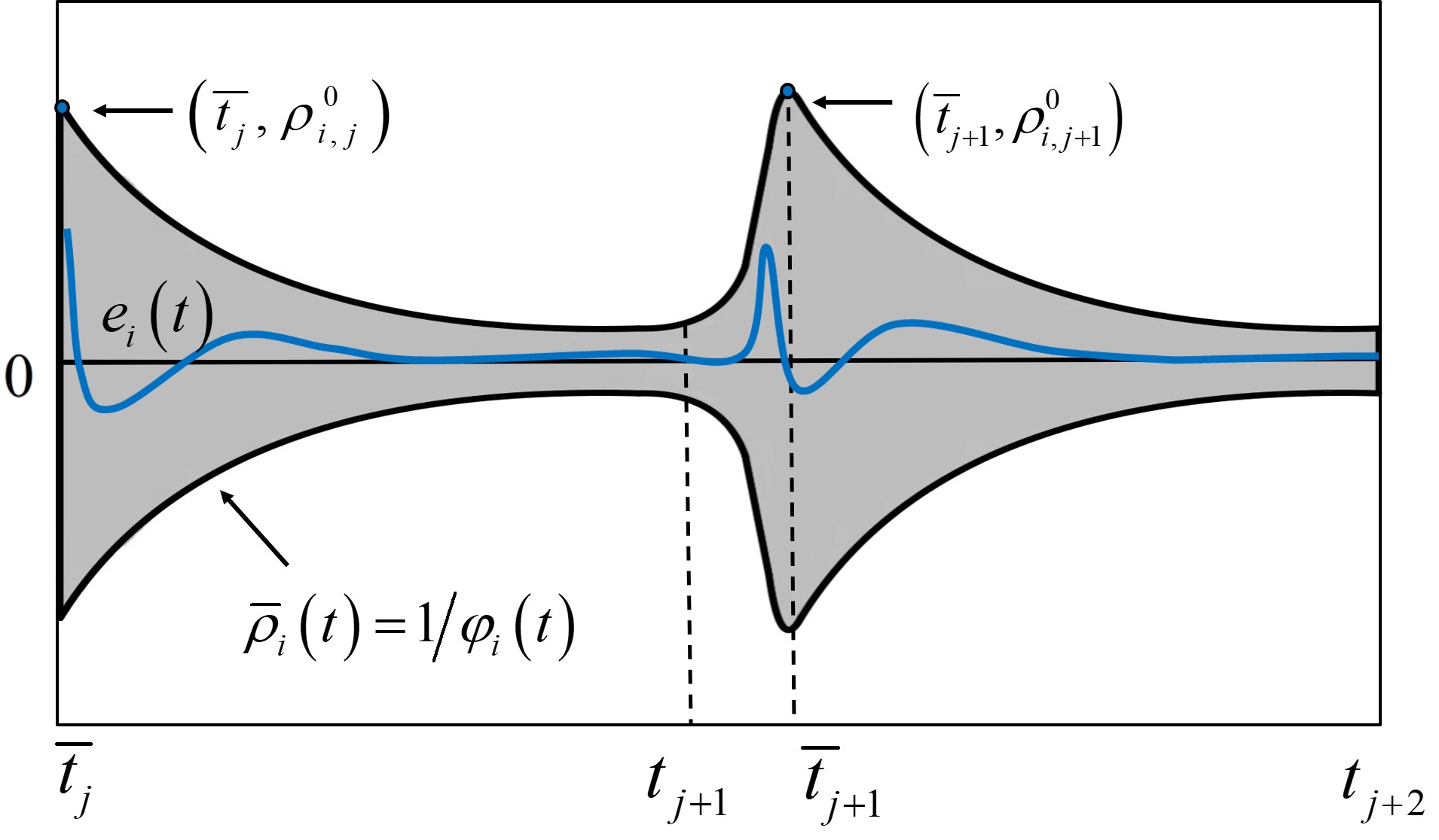
Figure 1: Tracking error evolution in the funnel Γφi(i=0,1,2,3)subscriptΓsubscript𝜑𝑖𝑖0123{\Gamma_{\varphi_{i}}}(i=0,1,2,3).

2.2 Funnel Boundary

We define functions φisubscript𝜑𝑖\varphi_{i} (i=0,1,2,3)𝑖0123(i=0,1,2,3) as the reciprocal of the funnel boundary ρ¯i(t)subscript¯𝜌𝑖𝑡{\bar{\rho}_{i}}\left(t\right), which describe the performance funnel ΓφisubscriptΓsubscript𝜑𝑖{\Gamma_{\varphi_{i}}} (cf. [19]) as

Γφi::subscriptΓsubscript𝜑𝑖absent\displaystyle{\Gamma_{\varphi_{i}}}: ={(t,ei)0×φi(t)|ei|<1}.absentconditional-set𝑡subscript𝑒𝑖subscriptabsent0subscript𝜑𝑖𝑡subscript𝑒𝑖1\displaystyle=\{\left({t,{e_{i}}}\right)\in{\mathbb{R}_{\geq 0}}\times\mathbb{R}\mid{\varphi_{i}}\left(t\right)|{e_{i}}|<1\}. (10)

The functions φisubscript𝜑𝑖\varphi_{i} are continuously differentiable, bounded with bounded derivatives, and satisfy φi(t)>0subscript𝜑𝑖𝑡0\varphi_{i}(t)>0 for all t0𝑡0t\geq 0 and lim inftφi(t)>0subscriptlimit-infimum𝑡subscript𝜑𝑖𝑡0\liminf_{t\to\infty}\varphi_{i}(t)>0. Fig. 1 displays the reciprocal ρ¯i(t)=1/φi(t)subscript¯𝜌𝑖𝑡1subscript𝜑𝑖𝑡\bar{\rho}_{i}(t)=1/\varphi_{i}(t).

In order to avoid peaks in the control input signal due to a strongly varying reference trajectory, we employ a non-monotonic funnel boundary defined as

1/φi(t)=ρ¯i(t)=1/subscript𝜑𝑖𝑡subscript¯𝜌𝑖𝑡absent\displaystyle{1\mathord{\left/{\vphantom{1{{\varphi_{i}}\left(t\right)}}}\right.\kern-1.2pt}{{\varphi_{i}}\left(t\right)}}={{\bar{\rho}}_{i}}\left(t\right)=
{ρ¯i,0(t)0t<t1ai,0(tt1)3+bi,0(tt1)2+ci,0(tt1)+di,0t1t<t¯1ρ¯i,1(t)t¯1t<t2ai,j1(ttj)3+bi,j1(ttj)2+ci,j1(ttj)+di,j1tjt<t¯jρ¯i,j(t)t¯jt<tj+1ai,p1(ttp)3+bi,p1(ttp)2+ci,p1(ttp)+di,p1tpt<t¯pρ¯i,p(t)t¯ptcasessubscript¯𝜌𝑖0𝑡0𝑡subscript𝑡1missing-subexpressionmissing-subexpressionmissing-subexpressionmissing-subexpressionmissing-subexpressionmissing-subexpressionmissing-subexpressionmissing-subexpressionmissing-subexpressionmissing-subexpressionmissing-subexpressionmissing-subexpressionmissing-subexpressionmissing-subexpressionmissing-subexpressionmissing-subexpressionmissing-subexpressionmissing-subexpressionsubscript𝑎𝑖0superscript𝑡subscript𝑡13subscript𝑏𝑖0superscript𝑡subscript𝑡12subscript𝑐𝑖0𝑡subscript𝑡1subscript𝑑𝑖0subscript𝑡1𝑡subscript¯𝑡1missing-subexpressionmissing-subexpressionmissing-subexpressionmissing-subexpressionmissing-subexpressionmissing-subexpressionmissing-subexpressionmissing-subexpressionmissing-subexpressionmissing-subexpressionmissing-subexpressionmissing-subexpressionmissing-subexpressionmissing-subexpressionmissing-subexpressionmissing-subexpressionmissing-subexpressionmissing-subexpressionsubscript¯𝜌𝑖1𝑡subscript¯𝑡1𝑡subscript𝑡2missing-subexpressionmissing-subexpressionmissing-subexpressionmissing-subexpressionmissing-subexpressionmissing-subexpressionmissing-subexpressionmissing-subexpressionmissing-subexpressionmissing-subexpressionmissing-subexpressionmissing-subexpressionmissing-subexpressionmissing-subexpressionmissing-subexpressionmissing-subexpressionmissing-subexpressionmissing-subexpressionmissing-subexpressionmissing-subexpressionmissing-subexpressionmissing-subexpressionmissing-subexpressionmissing-subexpressionmissing-subexpressionmissing-subexpressionmissing-subexpressionmissing-subexpressionmissing-subexpressionmissing-subexpressionmissing-subexpressionmissing-subexpressionmissing-subexpressionmissing-subexpressionmissing-subexpressionmissing-subexpressionsubscript𝑎𝑖𝑗1superscript𝑡subscript𝑡𝑗3subscript𝑏𝑖𝑗1superscript𝑡subscript𝑡𝑗2subscript𝑐𝑖𝑗1𝑡subscript𝑡𝑗subscript𝑑𝑖𝑗1missing-subexpressionmissing-subexpressionmissing-subexpressionmissing-subexpressionmissing-subexpressionmissing-subexpressionmissing-subexpressionmissing-subexpressionmissing-subexpressionmissing-subexpressionmissing-subexpressionmissing-subexpressionmissing-subexpressionmissing-subexpressionmissing-subexpressionmissing-subexpressionmissing-subexpressionmissing-subexpressionmissing-subexpressionsubscript𝑡𝑗𝑡subscript¯𝑡𝑗missing-subexpressionmissing-subexpressionmissing-subexpressionmissing-subexpressionmissing-subexpressionmissing-subexpressionmissing-subexpressionmissing-subexpressionmissing-subexpressionmissing-subexpressionmissing-subexpressionmissing-subexpressionmissing-subexpressionmissing-subexpressionmissing-subexpressionmissing-subexpressionmissing-subexpressionmissing-subexpressionsubscript¯𝜌𝑖𝑗𝑡subscript¯𝑡𝑗𝑡subscript𝑡𝑗1missing-subexpressionmissing-subexpressionmissing-subexpressionmissing-subexpressionmissing-subexpressionmissing-subexpressionmissing-subexpressionmissing-subexpressionmissing-subexpressionmissing-subexpressionmissing-subexpressionmissing-subexpressionmissing-subexpressionmissing-subexpressionmissing-subexpressionmissing-subexpressionmissing-subexpressionmissing-subexpressionmissing-subexpressionmissing-subexpressionmissing-subexpressionmissing-subexpressionmissing-subexpressionmissing-subexpressionmissing-subexpressionmissing-subexpressionmissing-subexpressionmissing-subexpressionmissing-subexpressionmissing-subexpressionmissing-subexpressionmissing-subexpressionmissing-subexpressionmissing-subexpressionmissing-subexpressionmissing-subexpressionsubscript𝑎𝑖𝑝1superscript𝑡subscript𝑡𝑝3subscript𝑏𝑖𝑝1superscript𝑡subscript𝑡𝑝2subscript𝑐𝑖𝑝1𝑡subscript𝑡𝑝subscript𝑑𝑖𝑝1subscript𝑡𝑝𝑡subscript¯𝑡𝑝missing-subexpressionmissing-subexpressionmissing-subexpressionmissing-subexpressionmissing-subexpressionmissing-subexpressionmissing-subexpressionmissing-subexpressionmissing-subexpressionmissing-subexpressionmissing-subexpressionmissing-subexpressionmissing-subexpressionmissing-subexpressionmissing-subexpressionmissing-subexpressionmissing-subexpressionmissing-subexpressionsubscript¯𝜌𝑖𝑝𝑡subscript¯𝑡𝑝𝑡missing-subexpressionmissing-subexpressionmissing-subexpressionmissing-subexpressionmissing-subexpressionmissing-subexpressionmissing-subexpressionmissing-subexpressionmissing-subexpressionmissing-subexpressionmissing-subexpressionmissing-subexpressionmissing-subexpressionmissing-subexpressionmissing-subexpressionmissing-subexpressionmissing-subexpressionmissing-subexpression\displaystyle\left\{{\begin{array}[]{*{20}{c}}{{{\bar{\rho}}_{i,0}}\left(t\right)}&{0\leq t<{t_{1}}}\\ \begin{array}[]{l}{a_{i,0}}{\left({t-{t_{1}}}\right)^{3}}+{b_{i,0}}{\left({t-{t_{1}}}\right)^{2}}\\ \;\;\;\;\;\;\;\;\;\;\;\;+{c_{i,0}}\left({t-{t_{1}}}\right)+{d_{i,0}}\end{array}&{{t_{1}}\leq t<{{\bar{t}}_{1}}}\\ {{{\bar{\rho}}_{i,1}}\left(t\right)}&{{{\bar{t}}_{1}}\leq t<{t_{2}}}\\ \vdots&\vdots\\ {\begin{array}[]{*{20}{l}}\begin{array}[]{l}{a_{i,j-1}}{\left({t-{t_{j}}}\right)^{3}}+{b_{i,j-1}}{\left({t-{t_{j}}}\right)^{2}}\\ \;\;\;\;\;\;\;\;\;\;\;\;+{c_{i,j-1}}\left({t-{t_{j}}}\right)+{d_{i,j-1}}\end{array}\end{array}}&{{t_{j}}\leq t<{{\bar{t}}_{j}}}\\ {{{\bar{\rho}}_{i,j}}\left(t\right)}&{{{\bar{t}}_{j}}\leq t<{t_{j+1}}}\\ \vdots&\vdots\\ \begin{array}[]{l}{a_{i,p-1}}{\left({t-{t_{p}}}\right)^{3}}+{b_{i,p-1}}{\left({t-{t_{p}}}\right)^{2}}\\ \;\;\;\;\;\;\;\;\;\;\;\;+{c_{i,p-1}}\left({t-{t_{p}}}\right)+{d_{i,p-1}}\end{array}&{{t_{p}}\leq t<{{\bar{t}}_{p}}}\\ {{{\bar{\rho}}_{i,p}}\left(t\right)}&{{{\bar{t}}_{p}}\leq t}\end{array}}\right. (27)

where tjsubscript𝑡𝑗t_{j} and t¯jsubscript¯𝑡𝑗\bar{t}_{j} (j=1,,p)𝑗1𝑝(j=1,...,p) are the triggered time and initial time points of every phase after maneuvering, t¯jtjsubscript¯𝑡𝑗subscript𝑡𝑗{{\bar{t}}_{j}}-{t_{j}} is the time range for maneuvering and p𝑝p represents the number of triggered times. The polynomials in each interval of the form [tj,t¯j]subscript𝑡𝑗subscript¯𝑡𝑗[t_{j},\bar{t}_{j}] are chosen based on the current maneuver encoded in the reference trajectory, and they ensure a widening of the funnel boundary. The functions ρ¯i,j(t)(i=0,1,2,3,j=1,2,,p)subscript¯𝜌𝑖𝑗𝑡formulae-sequence𝑖0123𝑗12𝑝{{{\bar{\rho}}_{i,j}}\left(t\right)}\;(i=0,1,2,3,j=1,2,...,p) are of the form

ρ¯i,j(t)=(ρi,j0ρi,j)eli,jt+ρi,jsubscript¯𝜌𝑖𝑗𝑡superscriptsubscript𝜌𝑖𝑗0superscriptsubscript𝜌𝑖𝑗superscript𝑒subscript𝑙𝑖𝑗𝑡superscriptsubscript𝜌𝑖𝑗\displaystyle{{\bar{\rho}}_{i,j}}\left(t\right)=\left({\rho_{i,j}^{0}-\rho_{i,j}^{\infty}}\right){e^{-{l_{i,j}}t}}+\rho_{i,j}^{\infty} (28)

with initial funnel width ρi,j0>0subscriptsuperscript𝜌0𝑖𝑗0{{\rho^{0}_{i,j}}}>0, required minimum exponential convergence rate li,j>0subscript𝑙𝑖𝑗0l_{i,j}>0 and the maximum steady state error ρi,j>0superscriptsubscript𝜌𝑖𝑗0\rho_{i,j}^{\infty}>0, respectively. In order to guarantee that ρ¯isubscript¯𝜌𝑖\bar{\rho}_{i} is continuously differentiable, the parameters ai,j,bi,j,ci,j,di,jsubscript𝑎𝑖𝑗subscript𝑏𝑖𝑗subscript𝑐𝑖𝑗subscript𝑑𝑖𝑗a_{i,j},b_{i,j},c_{i,j},d_{i,j} are chosen such that limttjρ¯i(t)=limttj+ρ¯i(t)subscript𝑡superscriptsubscript𝑡𝑗subscript¯𝜌𝑖𝑡subscript𝑡superscriptsubscript𝑡𝑗subscript¯𝜌𝑖𝑡\mathop{\lim}\limits_{t\to t_{j}^{-}}{{\bar{\rho}}_{i}}\left(t\right)=\mathop{\lim}\limits_{t\to t_{j}^{+}}{{\bar{\rho}}_{i}}\left(t\right), limtt¯jρ¯i(t)=limtt¯j+ρ¯i(t)subscript𝑡superscriptsubscript¯𝑡𝑗subscript¯𝜌𝑖𝑡subscript𝑡superscriptsubscript¯𝑡𝑗subscript¯𝜌𝑖𝑡\mathop{\lim}\limits_{t\to\bar{t}_{j}^{-}}{{\bar{\rho}}_{i}}\left(t\right)=\mathop{\lim}\limits_{t\to\bar{t}_{j}^{+}}{{\bar{\rho}}_{i}}\left(t\right), limttjρ¯˙i(t)=limttj+ρ¯˙i(t)subscript𝑡superscriptsubscript𝑡𝑗subscript˙¯𝜌𝑖𝑡subscript𝑡superscriptsubscript𝑡𝑗subscript˙¯𝜌𝑖𝑡\mathop{\lim}\limits_{t\to t_{j}^{-}}{{\dot{\bar{\rho}}}_{i}}\left(t\right)=\mathop{\lim}\limits_{t\to t_{j}^{+}}{{\dot{\bar{\rho}}}_{i}}\left(t\right), limtt¯jρ¯˙i(t)=limtt¯j+ρ¯˙i(t)subscript𝑡superscriptsubscript¯𝑡𝑗subscript˙¯𝜌𝑖𝑡subscript𝑡superscriptsubscript¯𝑡𝑗subscript˙¯𝜌𝑖𝑡\mathop{\lim}\limits_{t\to\bar{t}_{j}^{-}}{{\dot{\bar{\rho}}}_{i}}\left(t\right)=\mathop{\lim}\limits_{t\to\bar{t}_{j}^{+}}{{\dot{\bar{\rho}}}_{i}}\left(t\right) for j=1,,p𝑗1𝑝j=1,\ldots,p.

The proposed funnel boundary is displayed in Fig. 1 and we stress that it is different from the monotonically decreasing boundary functions of the form (28) widely used in [18], [20], [23]. Instead, it is a time triggered mechanism with trigger time points tjsubscript𝑡𝑗t_{j}, chosen in accordance with the reference trajectory, so that the proposed funnel (2.2) adapts itself and is suitable for the time-varying maneuvering command of RVs. For t>tp𝑡subscript𝑡𝑝t>t_{p} the novel funnel boundary converges to a neighbourhood of the origin, satisfying limtρ¯i(t)=ρi,p>0subscript𝑡subscript¯𝜌𝑖𝑡superscriptsubscript𝜌𝑖𝑝0\mathop{\lim}\limits_{t\to\infty}{{\bar{\rho}}_{i}}\left(t\right)=\rho_{i,p}^{\infty}>0.

2.3 Control Objective

The control objective is to design an output derivative feedback such that for any sufficiently smooth reference trajectory zhrefsubscript𝑧subscript𝑟𝑒𝑓{z_{h_{ref}}}, any initial values and under the influence of disturbances, the tracking error zhzhrefsubscript𝑧subscript𝑧subscript𝑟𝑒𝑓z_{h}-z_{h_{ref}} evolves within a prescribed performance funnel Γφ0subscriptΓsubscript𝜑0\Gamma_{\varphi_{0}} as in (10) and hence exhibits the desired transient and steady behavior. Furthermore, all signals u𝑢u, zhsubscript𝑧z_{h}, ψVsubscript𝜓𝑉\psi_{V}, ψ𝜓\psi, β𝛽\beta and ωysubscript𝜔𝑦\omega_{y} in the closed-loop system should remain bounded.

3 FUNNEL CONTROLLER DESIGN

3.1 Funnel-based control law design

Before we define the control law we introduce the following assumptions.

Assumption 1.

The reference trajectory zhrefsubscript𝑧subscript𝑟𝑒𝑓{z_{h_{ref}}} is known, it is four times continuously differentiable and its first four derivatives are bounded.

Assumption 2.

The disturbances ΔisubscriptΔ𝑖\Delta_{i} are measurable and essentially bounded with ΔiDisubscriptnormsubscriptΔ𝑖subscript𝐷𝑖\|\Delta_{i}\|_{\infty}\leq D_{i} for known constants Di0subscript𝐷𝑖0D_{i}\geq 0 (i=0,1,2,3)𝑖0123(i=0,1,2,3).

Assumptions 1 and 2 are reasonable and frequently used in the literature. The disturbances ΔisubscriptΔ𝑖\Delta_{i} (i=0,1,2,3)𝑖0123(i=0,1,2,3) involved in (1)-(5) account for uncertainties in the aerodynamic coefficients, noises and external disturbances, which are usually bounded throughout the flight process.

We define the tracking error as

e0(t)=y0(t)zhref(t)=zh(t)zhref(t)subscript𝑒0𝑡subscript𝑦0𝑡subscript𝑧subscript𝑟𝑒𝑓𝑡subscript𝑧𝑡subscript𝑧subscript𝑟𝑒𝑓𝑡e_{0}(t)=y_{0}(t)-{z_{h_{ref}}(t)}=z_{h}(t)-{z_{h_{ref}}(t)}

and introduce the following recursive structure

ei(t)=yi(t)zhref(i)(t)+ki1(t)ϖi1(t),i=1,2,3formulae-sequencesubscript𝑒𝑖𝑡subscript𝑦𝑖𝑡superscriptsubscript𝑧subscript𝑟𝑒𝑓𝑖𝑡subscript𝑘𝑖1𝑡subscriptitalic-ϖ𝑖1𝑡𝑖123\displaystyle{e_{i}}\left(t\right)={y_{i}}\left(t\right)-z_{{h_{ref}}}^{\left(i\right)}\left(t\right)+{k_{i-1}}\left(t\right){\varpi_{i-1}}\left(t\right),\ i=1,2,3 (29)

where ki(t)=11ϖi2(t)subscript𝑘𝑖𝑡11superscriptsubscriptitalic-ϖ𝑖2𝑡{k_{i}}\left(t\right)=\frac{1}{{1-\varpi_{i}^{2}\left(t\right)}} and ϖi(t)=φi(t)ei(t)subscriptitalic-ϖ𝑖𝑡subscript𝜑𝑖𝑡subscript𝑒𝑖𝑡{\varpi_{i}}\left(t\right)={\varphi_{i}}\left(t\right){e_{i}}\left(t\right) for φisubscript𝜑𝑖\varphi_{i} as in (2.2).

Then the funnel-based control law is given by

u(t)=k3(t)e3(t)=e3(t)1φ32(t)e32(t)𝑢𝑡subscript𝑘3𝑡subscript𝑒3𝑡subscript𝑒3𝑡1superscriptsubscript𝜑32𝑡superscriptsubscript𝑒32𝑡\displaystyle u\left(t\right)=-k_{3}\left(t\right){{e_{3}}\left(t\right)}=-\frac{{{e_{3}}\left(t\right)}}{{1-\varphi_{3}^{2}\left(t\right)e_{3}^{2}\left(t\right)}} (30)

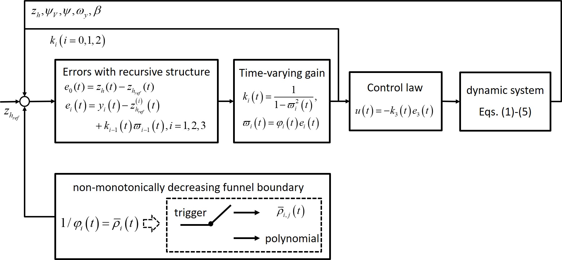
and the block diagram of the proposed control scheme is shown in Fig. 2.
Refer to caption
Figure 2: Funnel control structure for RV tracking issue.

In the sequel we investigate existence of solutions of the initial value problem resulting from the application of the funnel controller (30) to the RV with dynamics (1)-(5). By a solution of (1)-(5), (30) we mean a function (zh,ψV,ψ,ωy):[0,tf)4:subscript𝑧subscript𝜓𝑉𝜓subscript𝜔𝑦0subscript𝑡𝑓superscript4(z_{h},\psi_{V},\psi,\omega_{y}):[0,t_{f})\to\mathbb{R}^{4}, tf(0,]subscript𝑡𝑓0t_{f}\in(0,\infty], which is locally absolutely continuous and satisfies the initial conditions as well as the differential equations (1)-(5) for almost all t[0,tf)𝑡0subscript𝑡𝑓t\in[0,t_{f}). A solution is called maximal, if it has no right extension that is also a solution.

3.2 Stability Analysis

In this part, we present the stability analysis of the proposed control law.

Theorem 1.

Consider a RV with dynamics (1)-(5), satisfying Assumptions 1-2, under the funnel control law (30). Choose funnel boundaries φisubscript𝜑𝑖\varphi_{i} (i=0,1,2,3)𝑖0123(i=0,1,2,3) as in (2.2) such that the initial values satisfy

φi(0)|ei(0)|<1(i=0,1,2,3).subscript𝜑𝑖0subscript𝑒𝑖01𝑖0123\varphi_{i}(0)|e_{i}(0)|<1\quad(i=0,1,2,3).

Additionally, assume that the functions φ0,φ1subscript𝜑0subscript𝜑1\varphi_{0},\varphi_{1} and zhrefsubscript𝑧subscript𝑟𝑒𝑓z_{h_{ref}} satisfy the following condition:

μ(0,1)t0::𝜇01for-all𝑡0absent\displaystyle\exists\,\mu\in(0,1)\ \forall\,t\geq 0: (31)
|φ˙0(t)|Vφ02(t)+1φ1(t)+D0V+(1+V)V|z˙href(t)|μ.subscript˙𝜑0𝑡𝑉superscriptsubscript𝜑02𝑡1subscript𝜑1𝑡subscript𝐷0𝑉1𝑉𝑉subscript˙𝑧subscript𝑟𝑒𝑓𝑡𝜇\displaystyle\;\;\;\;\frac{{|{{\dot{\varphi}}_{0}}(t)|}}{{V\varphi_{0}^{2}(t)}}+\frac{1}{{{\varphi_{1}}(t)}}+\frac{{{D_{0}}}}{V}+\frac{{(1+V)}}{V}|{{\dot{z}}_{{h_{ref}}}}(t)|\leq\mu.

Then the funnel controller (30) applied to (1)-(5) yields an initial-value problem which has a solution, every solution can be maximally extended and every maximal solution (zh,ψV,ψ,ωy):[0,tf)4:subscript𝑧subscript𝜓𝑉𝜓subscript𝜔𝑦0subscript𝑡𝑓superscript4(z_{h},\psi_{V},\psi,\omega_{y}):[0,t_{f})\to\mathbb{R}^{4}, tf(0,]subscript𝑡𝑓0t_{f}\in(0,\infty] has the following properties:

  • global existence: tf=subscript𝑡𝑓t_{f}=\infty;

  • all errors evolve uniformly in the respective prescribed performance funnels, that is for all i=0,1,2,3𝑖0123i=0,1,2,3 there exists εi(0,1)subscript𝜀𝑖01{\varepsilon_{i}}\in(0,1) such that for all t0𝑡0t\geq 0 we have |ϖi(t)|εisubscriptitalic-ϖ𝑖𝑡subscript𝜀𝑖|{\varpi_{i}}\left(t\right)|\leq{\varepsilon_{i}}.

  • all signals zhsubscript𝑧z_{h}, ψVsubscript𝜓𝑉\psi_{V}, ψ𝜓\psi, ωysubscript𝜔𝑦\omega_{y}, δysubscript𝛿𝑦\delta_{y} and kisubscript𝑘𝑖k_{i} (i=0,1,2,3)𝑖0123(i=0,1,2,3) in the closed-loop system are bounded.

Proof.

Before the analysis, we record that it follows from (6)-(9) that the derivatives of ei(t)subscript𝑒𝑖𝑡e_{i}(t) (i=0,1,2,3)𝑖0123(i=0,1,2,3) can be expressed as

e˙0(t)subscript˙𝑒0𝑡\displaystyle{{\dot{e}}_{0}}\left(t\right) =Vsin(y1(t))z˙href(t)+Δ0(t)absent𝑉subscript𝑦1𝑡subscript˙𝑧subscript𝑟𝑒𝑓𝑡subscriptΔ0𝑡\displaystyle=-V\sin\left({{y_{1}}\left(t\right)}\right)-{{\dot{z}}_{{h_{ref}}}}\left(t\right)+{\Delta_{0}}(t) (32)
e˙1(t)subscript˙𝑒1𝑡\displaystyle{{\dot{e}}_{1}}\left(t\right) =e2(t)k1(t)ϖ1(t)+ddt(k0(t)ϖ0(t))absentsubscript𝑒2𝑡subscript𝑘1𝑡subscriptitalic-ϖ1𝑡𝑑𝑑𝑡subscript𝑘0𝑡subscriptitalic-ϖ0𝑡\displaystyle={e_{2}}\left(t\right)-{k_{1}}\left(t\right){\varpi_{1}}\left(t\right)+\frac{d}{{dt}}\left({{k_{0}}\left(t\right){\varpi_{0}}\left(t\right)}\right)
(1+c2)y2(t)c1+Δ1(t)1subscript𝑐2subscript𝑦2𝑡subscript𝑐1subscriptΔ1𝑡\displaystyle\;\;\;\;-(1+c_{2}){y_{2}}\left(t\right)-{c_{1}}+{\Delta_{1}}(t) (33)
e˙2(t)subscript˙𝑒2𝑡\displaystyle{{\dot{e}}_{2}}\left(t\right) =e3(t)k2(t)ϖ2(t)+ddt(k1(t)ϖ1(t))absentsubscript𝑒3𝑡subscript𝑘2𝑡subscriptitalic-ϖ2𝑡𝑑𝑑𝑡subscript𝑘1𝑡subscriptitalic-ϖ1𝑡\displaystyle={e_{3}}\left(t\right)-{k_{2}}\left(t\right){\varpi_{2}}\left(t\right)+\frac{d}{{dt}}\left({{k_{1}}\left(t\right){\varpi_{1}}\left(t\right)}\right)
+c1+c2y2(t)+Δ2(t)Δ1(t)subscript𝑐1subscript𝑐2subscript𝑦2𝑡subscriptΔ2𝑡subscriptΔ1𝑡\displaystyle\;\;\;\;+{c_{1}}+{c_{2}}{y_{2}}\left(t\right)+{\Delta_{2}}(t)-{\Delta_{1}}(t) (34)
e˙3(t)subscript˙𝑒3𝑡\displaystyle{{\dot{e}}_{3}}\left(t\right) =c5u(t)zhref(4)(t)+ddt(k2(t)ϖ2(t))absentsubscript𝑐5𝑢𝑡superscriptsubscript𝑧subscript𝑟𝑒𝑓4𝑡𝑑𝑑𝑡subscript𝑘2𝑡subscriptitalic-ϖ2𝑡\displaystyle={c_{5}}u\left(t\right)-z_{{h_{ref}}}^{\left(4\right)}\left(t\right)+\frac{d}{{dt}}\left({{k_{2}}\left(t\right){\varpi_{2}}\left(t\right)}\right)
+c3+c4y2(t)+Δ3(t)subscript𝑐3subscript𝑐4subscript𝑦2𝑡subscriptΔ3𝑡\displaystyle\;\;\;\;+{c_{3}}+{c_{4}}{y_{2}}\left(t\right)+{\Delta_{3}}(t) (35)

In the following, we will first show that a local solution exists on [0,tf)0subscript𝑡𝑓[0,t_{f}) and the tracking error evolves uniformly within the prescribed performance funnel, and we show tf=subscript𝑡𝑓t_{f}=\infty in the last step.

Step 1: To show existence of a solution of the closed-loop system, consider the functions

e~0:D0,(t,y0)y0zhref(t):subscript~𝑒0formulae-sequencesubscript𝐷0maps-to𝑡subscript𝑦0subscript𝑦0subscript𝑧subscript𝑟𝑒𝑓𝑡\displaystyle{{\tilde{e}}_{0}}:{D_{0}}\to\mathbb{R},\ \left({t,{y_{0}}}\right)\mapsto{y_{0}}-{z_{h_{ref}}}(t) (36)

with the set D0:=0×assignsubscript𝐷0subscriptabsent0{D_{0}}:={\mathbb{R}_{\geq 0}}\times\mathbb{R} and

e~i:Di,(t,y0,,yi)yizhref(i)(t):subscript~𝑒𝑖formulae-sequencesubscript𝐷𝑖maps-to𝑡subscript𝑦0subscript𝑦𝑖subscript𝑦𝑖superscriptsubscript𝑧subscript𝑟𝑒𝑓𝑖𝑡\displaystyle{{\tilde{e}}_{i}}:{D_{i}}\to\mathbb{R},\ \left({t,{y_{0}},\ldots,{y_{i}}}\right)\mapsto{y_{i}}-z_{h_{ref}}^{(i)}(t) (37)
+φi1(t)e~i1(t,y0,,yi1)1φi12(t)e~i12(t,y0,,yi1)subscript𝜑𝑖1𝑡subscript~𝑒𝑖1𝑡subscript𝑦0subscript𝑦𝑖11superscriptsubscript𝜑𝑖12𝑡superscriptsubscript~𝑒𝑖12𝑡subscript𝑦0subscript𝑦𝑖1\displaystyle\;\;\;\;\;\;\;\;\;\;\;\;\;+\frac{{{\varphi_{i-1}}(t){{\tilde{e}}_{i-1}}(t,{y_{0}},\ldots,{y_{i-1}})}}{{1-\varphi_{i-1}^{2}(t)\tilde{e}_{i-1}^{2}(t,{y_{0}},\ldots,{y_{i-1}})}}

with the sets

Di:={(t,y0,,yi)Di1×\displaystyle{D_{i}}:=\left\{{\left({t,{y_{0}},\ldots,{y_{i}}}\right)\in{D_{i-1}}\times\mathbb{R}\mid}\right. (38)
φi1(t)|e~i1(t,y0,,yi)|<1},(i=1,2,3),\displaystyle\;\;\;\;\;{\varphi_{i-1}}(t)|{{\tilde{e}}_{i-1}}\left({t,{y_{0}},\ldots,{y_{i}}}\right)|<1\},\ \left({i=1,2,3}\right),
D4:={(t,y0,,y3)D3\displaystyle{D_{4}}:=\left\{{\left({t,{y_{0}},\ldots,{y_{3}}}\right)\in{D_{3}}\mid}\right.
φ3(t)|e~3(t,y0,,y3)|<1}.\displaystyle\;\;\;\;\;{\varphi_{3}}(t)|{{\tilde{e}}_{3}}\left({t,{y_{0}},\ldots,{y_{3}}}\right)|<1\}.

Introducing Y(t)=(y0(t),,y3(t))𝑌𝑡superscriptsubscript𝑦0𝑡subscript𝑦3𝑡topY(t)=(y_{0}(t),\ldots,y_{3}(t))^{\top} and the function

F:D44,(t,y0,,y3):𝐹subscript𝐷4superscript4𝑡subscript𝑦0subscript𝑦3\displaystyle F:{D_{4}}\to{\mathbb{R}^{4}},\;(t,{y_{0}},\ldots,{y_{3}}) (39)
(Vsin(y1)+Δ0(t)c1c2y2+Δ1(t)y3+c1+c2y2+Δ2(t)Δ1(t)c3+c4y2+Δ3(t)c5φ3(t)e~3(t,y0,,y3)1φ32(t)e~(t,y0,,y3)32)\displaystyle\mapsto\left({\begin{array}[]{*{20}{c}}{-V\sin({y_{1}})+{\Delta_{0}}}(t)\\ {-{c_{1}}-{c_{2}}{y_{2}}+{\Delta_{1}}}(t)\\ {{y_{3}}+{c_{1}}+{c_{2}}{y_{2}}+{\Delta_{2}}(t)-{\Delta_{1}}}(t)\\ {{c_{3}}+{c_{4}}{y_{2}}+{\Delta_{3}}(t)-{c_{5}}\frac{{{\varphi_{3}}(t){{\tilde{e}}_{3}}(t,{y_{0}},\ldots,{y_{3}})}}{{1-\varphi_{3}^{2}(t)\tilde{e}{{{}_{3}^{2}}}(t,{y_{0}},\ldots,{y_{3}})}}}\end{array}}\right)

the closed-loop system takes the form

Y˙(t)=F(t,Y(t)),Y(0)=(y00,,y30).formulae-sequence˙𝑌𝑡𝐹𝑡𝑌𝑡𝑌0superscriptsuperscriptsubscript𝑦00superscriptsubscript𝑦30top\dot{Y}(t)=F(t,Y(t)),\quad Y(0)=(y_{0}^{0},\ldots,y_{3}^{0})^{\top}. (40)

Since (0,Y(0))D40𝑌0subscript𝐷4(0,Y(0))\in D_{4} and F𝐹F is measurable in t𝑡t, continuous in (y0,,y3)subscript𝑦0subscript𝑦3(y_{0},\ldots,y_{3}) and locally essentially bounded, an application of Theorem B.1 from [29] yields the existence of a solution and every solution can be extended to a maximal solution Y:[0,tf)4:𝑌0subscript𝑡𝑓superscript4Y:[0,t_{f})\to\mathbb{R}^{4} with tf(0,]subscript𝑡𝑓0t_{f}\in(0,\infty]. Furthermore, the graph of Y𝑌Y is not a compact subset of D4subscript𝐷4D_{4}.

Step 2: We show that k0subscript𝑘0k_{0} is bounded on [0,tf)0subscript𝑡𝑓[0,t_{f}). According to the definition of ϖ0(t)subscriptitalic-ϖ0𝑡\varpi_{0}(t) and (32) we have

ϖ˙0(t)subscript˙italic-ϖ0𝑡\displaystyle{{\dot{\varpi}}_{0}}\left(t\right) =φ˙0(t)φ0(t)ϖ0(t)φ0(t)Vsin(y1(t))absentsubscript˙𝜑0𝑡subscript𝜑0𝑡subscriptitalic-ϖ0𝑡subscript𝜑0𝑡𝑉subscript𝑦1𝑡\displaystyle=\frac{{{{\dot{\varphi}}_{0}}\left(t\right)}}{{{\varphi_{0}}\left(t\right)}}{\varpi_{0}}\left(t\right)-{\varphi_{0}}\left(t\right)V\sin\left({{y_{1}}\left(t\right)}\right) (41)
+φ0(t)(Δ0(t)z˙href(t)).subscript𝜑0𝑡subscriptΔ0𝑡subscript˙𝑧subscript𝑟𝑒𝑓𝑡\displaystyle+{\varphi_{0}}\left(t\right)\left({{\Delta_{0}}(t)-{{\dot{z}}_{{h_{ref}}}}\left(t\right)}\right).

By the mean value theorem, for each t[0,tf)𝑡0subscript𝑡𝑓t\in[0,t_{f}), there exists ξ(t)𝜉𝑡\xi\left(t\right) between k0(t)ϖ0(t)subscript𝑘0𝑡subscriptitalic-ϖ0𝑡-{k_{0}}\left(t\right){\varpi_{0}}\left(t\right) and k0(t)ϖ0(t)+e1(t)+z˙href(t)subscript𝑘0𝑡subscriptitalic-ϖ0𝑡subscript𝑒1𝑡subscript˙𝑧subscript𝑟𝑒𝑓𝑡-{k_{0}}\left(t\right){\varpi_{0}}\left(t\right)+{e_{1}}\left(t\right)+{{\dot{z}}_{{h_{ref}}}}\left(t\right) such that

sin(y1(t))subscript𝑦1𝑡\displaystyle\sin\left({{y_{1}}\left(t\right)}\right) =sin(k0(t)ϖ0(t)+e1(t)+z˙href(t))absentsubscript𝑘0𝑡subscriptitalic-ϖ0𝑡subscript𝑒1𝑡subscript˙𝑧subscript𝑟𝑒𝑓𝑡\displaystyle=\sin\left({-{k_{0}}\left(t\right){\varpi_{0}}\left(t\right)+{e_{1}}\left(t\right)+{{\dot{z}}_{{h_{ref}}}}\left(t\right)}\right) (42)
=sin(k0(t)ϖ0(t))absentsubscript𝑘0𝑡subscriptitalic-ϖ0𝑡\displaystyle=\sin\left({-{k_{0}}\left(t\right){\varpi_{0}}\left(t\right)}\right)
+(e1(t)+z˙href(t))cos(ξ(t)).subscript𝑒1𝑡subscript˙𝑧subscript𝑟𝑒𝑓𝑡𝜉𝑡\displaystyle+\left({{e_{1}}\left(t\right)+{{\dot{z}}_{{h_{ref}}}}\left(t\right)}\right)\cos\left({\xi\left(t\right)}\right).

Now define U0(t)=12ϖ02(t)subscript𝑈0𝑡12superscriptsubscriptitalic-ϖ02𝑡{U_{0}}(t)=\frac{1}{2}\varpi_{0}^{2}\left(t\right), then from (31), (41) and (42), and invoking |ϖ0(t)|<1subscriptitalic-ϖ0𝑡1|{{\varpi_{0}}\left(t\right)}|<1 and |e1(t)|<1/φ1(t)subscript𝑒1𝑡1subscript𝜑1𝑡|e_{1}(t)|<1/\varphi_{1}(t), we find that

U˙0(t)=ϖ0(t)ϖ˙0(t)subscript˙𝑈0𝑡subscriptitalic-ϖ0𝑡subscript˙italic-ϖ0𝑡\displaystyle{\dot{U}_{0}}(t)={\varpi_{0}}\left(t\right){{\dot{\varpi}}_{0}}\left(t\right) (43)
=φ˙0(t)φ0(t)ϖ02(t)+φ0(t)ϖ0(t)(Vsin(k0(t)ϖ0(t))\displaystyle=\frac{{{{\dot{\varphi}}_{0}}(t)}}{{{\varphi_{0}}(t)}}{\varpi_{0}^{2}}{\left(t\right)}+{\varphi_{0}}\left(t\right){\varpi_{0}}\left(t\right)(-V\sin(-{k_{0}}(t){\varpi_{0}}\left(t\right))
V(e1(t)+z˙href(t))cos(ξ(t))+Δ0(t)z˙href(t))\displaystyle\;\;\;\;-V({e_{1}}(t)+{{\dot{z}}_{{h_{ref}}}}(t))\cos(\xi(t))+{\Delta_{0}}(t)-{{\dot{z}}_{{h_{ref}}}}(t))
Vφ0(t)sin(k0(t)ϖ0(t))ϖ0(t)+|φ˙0(t)|φ0(t)absent𝑉subscript𝜑0𝑡subscript𝑘0𝑡subscriptitalic-ϖ0𝑡subscriptitalic-ϖ0𝑡subscript˙𝜑0𝑡subscript𝜑0𝑡\displaystyle\leq-V{\varphi_{0}}(t)\sin\left({-{k_{0}}(t){\varpi_{0}}\left(t\right)}\right){\varpi_{0}}\left(t\right)+\frac{{|{{\dot{\varphi}}_{0}}(t)|}}{{{\varphi_{0}}(t)}}
+Vφ0(t)(1φ1(t)+D0V+(1+V)V|z˙href(t)|)𝑉subscript𝜑0𝑡1subscript𝜑1𝑡subscript𝐷0𝑉1𝑉𝑉subscript˙𝑧subscript𝑟𝑒𝑓𝑡\displaystyle\;\;\;\;+V{\varphi_{0}}(t)\left({\frac{1}{{{\varphi_{1}}(t)}}+\frac{{{D_{0}}}}{V}+\frac{{(1+V)}}{V}|{{\dot{z}}_{{h_{ref}}}}(t)|}\right)
Vφ0(t)(N(ϖ0(t))+μ)absent𝑉subscript𝜑0𝑡𝑁subscriptitalic-ϖ0𝑡𝜇\displaystyle\leq V{\varphi_{0}}(t)\left(-N(-{\varpi_{0}}\left(t\right))+\mu\right)

where N:(1,1)(1,1),ssin(s1s2)s:𝑁formulae-sequence1111maps-to𝑠𝑠1superscript𝑠2𝑠N:(-1,1)\to(-1,1),\ s\mapsto\sin\left(\tfrac{s}{1-s^{2}}\right)s. The function N𝑁N is symmetric and satisfies N(s)=N(s)𝑁𝑠𝑁𝑠N(-s)=N(s).

Choose ε0(0,1)subscript𝜀001\varepsilon_{0}\in(0,1) such that |ϖ0(0)|<ε0subscriptitalic-ϖ00subscript𝜀0|\varpi_{0}(0)|<\varepsilon_{0} and N(ε0)<μ𝑁subscript𝜀0𝜇N(\varepsilon_{0})<-\mu. In the following, we show that |ϖ0(t)|ε0subscriptitalic-ϖ0𝑡subscript𝜀0|\varpi_{0}(t)|\leq\varepsilon_{0} for all t[0,tf)𝑡0subscript𝑡𝑓t\in[0,t_{f}). Assume there exists some t[0,tf)𝑡0subscript𝑡𝑓t\in[0,t_{f}) with |ϖ0(t)|>ε0subscriptitalic-ϖ0𝑡subscript𝜀0|\varpi_{0}(t)|>\varepsilon_{0} and define

t¯0:=inf{t[0,tf)|ϖ0(t)|>ε0}>0.assignsubscript¯𝑡0infimumconditional-set𝑡0subscript𝑡𝑓subscriptitalic-ϖ0𝑡subscript𝜀00{{\bar{t}}_{0}}:=\inf\left\{{t\in[0,{\color[rgb]{0,0,0}t_{f}})\mid\left|{{\varpi_{0}}(t)|>\varepsilon_{0}}\right.}\right\}>0.

Since N𝑁N is continuous there exists η>0𝜂0\eta>0 such that N(s)μ𝑁𝑠𝜇N(s)\leq-\mu for all s𝑠s\in\mathbb{R} with |sε0|η𝑠subscript𝜀0𝜂|s-\varepsilon_{0}|\leq\eta. By symmetry of N𝑁N we also have N(s)μ𝑁𝑠𝜇N(s)\leq-\mu for all s𝑠s\in\mathbb{R} with |s+ε0|η𝑠subscript𝜀0𝜂|s+\varepsilon_{0}|\leq\eta. Since ϖ0subscriptitalic-ϖ0\varpi_{0} is continuous with |ϖ0(t¯0)|=ε0subscriptitalic-ϖ0subscript¯𝑡0subscript𝜀0|\varpi_{0}(\bar{t}_{0})|=\varepsilon_{0}, there exists t¯1(t¯0,tf)subscript¯𝑡1subscript¯𝑡0subscript𝑡𝑓\bar{t}_{1}\in(\bar{t}_{0},t_{f}) such that |ϖ0(t)|>ε0subscriptitalic-ϖ0𝑡subscript𝜀0|\varpi_{0}(t)|>\varepsilon_{0} and |ϖ0(t¯0)ϖ0(t)|<ηsubscriptitalic-ϖ0subscript¯𝑡0subscriptitalic-ϖ0𝑡𝜂|\varpi_{0}(\bar{t}_{0})-\varpi_{0}(t)|<\eta for all t(t¯0,t¯1]𝑡subscript¯𝑡0subscript¯𝑡1t\in(\bar{t}_{0},\bar{t}_{1}].

Let σ=sgnϖ0(t¯0)𝜎sgnsubscriptitalic-ϖ0subscript¯𝑡0\sigma=\mathop{\rm sgn}\varpi_{0}(\bar{t}_{0}), then ϖ0(t¯0)=σ|ϖ0(t¯0)|=σε0subscriptitalic-ϖ0subscript¯𝑡0𝜎subscriptitalic-ϖ0subscript¯𝑡0𝜎subscript𝜀0\varpi_{0}(\bar{t}_{0})=\sigma|\varpi_{0}(\bar{t}_{0})|=\sigma\varepsilon_{0} and hence |ϖ0(t)ϖ0(t¯0)|=|ϖ0(t)σε0|ηsubscriptitalic-ϖ0𝑡subscriptitalic-ϖ0subscript¯𝑡0subscriptitalic-ϖ0𝑡𝜎subscript𝜀0𝜂|\varpi_{0}(t)-\varpi_{0}(\bar{t}_{0})|=|\varpi_{0}(t)-\sigma\varepsilon_{0}|\leq\eta for all t[t¯0,t¯1]𝑡subscript¯𝑡0subscript¯𝑡1t\in[\bar{t}_{0},\bar{t}_{1}]. It follows that N(ϖ0(t))μ𝑁subscriptitalic-ϖ0𝑡𝜇N(\varpi_{0}(t))\leq-\mu for all t[t¯0,t¯1]𝑡subscript¯𝑡0subscript¯𝑡1t\in[\bar{t}_{0},\bar{t}_{1}], and hence U˙0(t)Vφ0(t)(N(ϖ0(t))+μ)0subscript˙𝑈0𝑡𝑉subscript𝜑0𝑡𝑁subscriptitalic-ϖ0𝑡𝜇0{\dot{U}_{0}}(t)\leq V\varphi_{0}(t)\big{(}{\color[rgb]{0,0,0}N(\varpi_{0}(t))}+\mu\big{)}\leq 0, which upon integration gives ε02=ϖ0(t¯0)2ϖ0(t¯1)2>ε02superscriptsubscript𝜀02subscriptitalic-ϖ0superscriptsubscript¯𝑡02subscriptitalic-ϖ0superscriptsubscript¯𝑡12superscriptsubscript𝜀02\varepsilon_{0}^{2}=\varpi_{0}(\bar{t}_{0})^{2}\geq\varpi_{0}(\bar{t}_{1})^{2}>\varepsilon_{0}^{2}, a contradiction. Hence, |ϖ0(t)|ε0subscriptitalic-ϖ0𝑡subscript𝜀0|\varpi_{0}(t)|\leq\varepsilon_{0} for all t[0,tf)𝑡0subscript𝑡𝑓t\in[0,t_{f}) and thus k0subscript𝑘0k_{0} is bounded on [0,tf)0subscript𝑡𝑓[0,t_{f}).

Step 3: We show that k1subscript𝑘1k_{1} is bounded on [0,tf)0subscript𝑡𝑓[0,t_{f}). A standard procedure in funnel control is used by seeking a contradiction. For some ε1(0,1)subscript𝜀101\varepsilon_{1}\in(0,1), which we will determine later, suppose that there exists t1[0,tf)superscriptsubscript𝑡10subscript𝑡𝑓t_{1}^{*}\in[0,t_{f}) such that ϖ1(t1)>ε1subscriptitalic-ϖ1superscriptsubscript𝑡1subscript𝜀1{\varpi_{1}}\left(t_{1}^{*}\right)>\varepsilon_{1} and define

t0:=max{t[0,t1)ϖ1(t)=ε1}.assignsuperscriptsubscript𝑡0𝑡conditional0superscriptsubscript𝑡1subscriptitalic-ϖ1𝑡subscript𝜀1t_{0}^{*}:=\max\{t\in[0,t_{1}^{*})\mid{\varpi_{1}}\left(t\right)=\varepsilon_{1}\}.

Then we find that

t[t0,t1]:ϖ1(t)ε1:for-all𝑡superscriptsubscript𝑡0superscriptsubscript𝑡1subscriptitalic-ϖ1𝑡subscript𝜀1\displaystyle\forall\,t\in\left[{t_{0}^{*},t_{1}^{*}}\right]:\ {\varpi_{1}}\left(t\right)\geq{\varepsilon_{1}} (44)

and hence

t[t0,t1]:k1(t)=11ϖ12(t)11ε12.:for-all𝑡superscriptsubscript𝑡0superscriptsubscript𝑡1subscript𝑘1𝑡11superscriptsubscriptitalic-ϖ12𝑡11superscriptsubscript𝜀12\displaystyle\forall\,t\in\left[{t_{0}^{*},t_{1}^{*}}\right]:\ {k_{1}}\left(t\right)=\frac{1}{{1-\varpi_{1}^{2}\left(t\right)}}\geq\frac{1}{{1-\varepsilon_{1}^{2}}}. (45)

Define U1(t)=12ϖ12(t)subscript𝑈1𝑡12superscriptsubscriptitalic-ϖ12𝑡{U_{1}}(t)=\frac{1}{2}\varpi_{1}^{2}\left(t\right), then according to (3.2) we have

U˙1(t)=ϖ1(t)ϖ˙1(t)subscript˙𝑈1𝑡subscriptitalic-ϖ1𝑡subscript˙italic-ϖ1𝑡\displaystyle{{\dot{U}}_{1}}(t)={\varpi_{1}}\left(t\right){{\dot{\varpi}}_{1}}\left(t\right) (46)
=ϖ1(t)(φ˙1(t)e1(t)+φ1(t)e˙1(t))absentsubscriptitalic-ϖ1𝑡subscript˙𝜑1𝑡subscript𝑒1𝑡subscript𝜑1𝑡subscript˙𝑒1𝑡\displaystyle={\varpi_{1}}\left(t\right)\left({{{\dot{\varphi}}_{1}}\left(t\right){e_{1}}\left(t\right)+{\varphi_{1}}\left(t\right){{\dot{e}}_{1}}\left(t\right)}\right)
=φ˙1(t)φ1(t)ϖ12(t)φ1(t)k1(t)ϖ12(t)c1φ1(t)ϖ1(t)absentsubscript˙𝜑1𝑡subscript𝜑1𝑡superscriptsubscriptitalic-ϖ12𝑡subscript𝜑1𝑡subscript𝑘1𝑡superscriptsubscriptitalic-ϖ12𝑡subscript𝑐1subscript𝜑1𝑡subscriptitalic-ϖ1𝑡\displaystyle=\frac{{{{\dot{\varphi}}_{1}}(t)}}{{{\varphi_{1}}(t)}}{\varpi_{1}^{2}}{(t)}-{\varphi_{1}}(t){k_{1}}(t){\varpi_{1}^{2}}{(t)}-{c_{1}}{\varphi_{1}}(t){\varpi_{1}}(t)
+φ1(t)ϖ1(t)(c2y2(t)+Δ1(t)+e2(t)y2(t))subscript𝜑1𝑡subscriptitalic-ϖ1𝑡subscript𝑐2subscript𝑦2𝑡subscriptΔ1𝑡subscript𝑒2𝑡subscript𝑦2𝑡\displaystyle\;\;\;\;+{\varphi_{1}}(t){\varpi_{1}}(t)\left({-{c_{2}}{y_{2}}(t)+{\Delta_{1}}(t)+{e_{2}}(t)-{y_{2}}(t)}\right)
+φ1(t)ϖ1(t)(1+2ϖ02(t)k0(t))k0(t)ϖ˙0(t).subscript𝜑1𝑡subscriptitalic-ϖ1𝑡12superscriptsubscriptitalic-ϖ02𝑡subscript𝑘0𝑡subscript𝑘0𝑡subscript˙italic-ϖ0𝑡\displaystyle{\color[rgb]{0,0,0}\;\;\;\;+{\varphi_{1}}(t){\varpi_{1}}(t)\left({1+2{\varpi_{0}^{2}}{{(t)}}{k_{0}}\left(t\right)}\right){k_{0}}(t){{\dot{\varpi}}_{0}}(t)}.

From Step 2 we have that k0subscript𝑘0k_{0} is bounded on t[0,tf)𝑡0subscript𝑡𝑓t\in[0,t_{f}). Furthermore, ϖ˙0subscript˙italic-ϖ0\dot{\varpi}_{0} is bounded by (41), |e2(t)|<1/φ2(t)subscript𝑒2𝑡1subscript𝜑2𝑡|e_{2}(t)|<1/\varphi_{2}(t) and y2,Δ1,φ1,φ˙1subscript𝑦2subscriptΔ1subscript𝜑1subscript˙𝜑1y_{2},\Delta_{1},\varphi_{1},\dot{\varphi}_{1} are clearly bounded as well, hence there exists an upper bound C1>0subscript𝐶10C_{1}>0 such that for all t[0,tf)𝑡0subscript𝑡𝑓t\in[0,t_{f}) we have

|φ˙1(t)|φ12(t)+c1+(1+c2)|y2(t)|+|Δ1(t)|+|e2(t)|subscript˙𝜑1𝑡superscriptsubscript𝜑12𝑡subscript𝑐11subscript𝑐2subscript𝑦2𝑡subscriptΔ1𝑡subscript𝑒2𝑡\displaystyle\ \frac{|\dot{\varphi}_{1}(t)|}{\varphi_{1}^{2}(t)}+c_{1}+(1+c_{2})|y_{2}(t)|+|\Delta_{1}(t)|+|e_{2}(t)| (47)
+(1+2ϖ02(t)k0(t))k0(t)ϖ˙0(t)C1.12superscriptsubscriptitalic-ϖ02𝑡subscript𝑘0𝑡subscript𝑘0𝑡subscript˙italic-ϖ0𝑡subscript𝐶1\displaystyle{\color[rgb]{0,0,0}+\left({1+2{\varpi_{0}^{2}}{{(t)}}{k_{0}}\left(t\right)}\right){k_{0}}(t){{\dot{\varpi}}_{0}}(t)\leq C_{1}}.

Invoking |ϖ1(t)|<1subscriptitalic-ϖ1𝑡1|{{\varpi_{1}}\left(t\right)}|<1 we thus obtain

U˙1(t)subscript˙𝑈1𝑡\displaystyle{{\dot{U}}_{1}}(t) φ1(t)|ϖ1(t)|(k1(t)|ϖ1(t)|+C1)0absentsubscript𝜑1𝑡subscriptitalic-ϖ1𝑡subscript𝑘1𝑡subscriptitalic-ϖ1𝑡subscript𝐶10\displaystyle\leq{\varphi_{1}}(t)|{\varpi_{1}}(t)|\left({-{k_{1}}(t)|{\varpi_{1}}(t)|+C_{1}}\right){\color[rgb]{0,0,0}\leq 0} (48)

when we choose ε1(0,1)subscript𝜀101\varepsilon_{1}\in(0,1) large enough so that ε11ε12C1subscript𝜀11superscriptsubscript𝜀12subscript𝐶1\frac{\varepsilon_{1}}{1-\varepsilon_{1}^{2}}\geq C_{1}. Upon integration over [t0,t1]superscriptsubscript𝑡0superscriptsubscript𝑡1[t_{0}^{*},t_{1}^{*}] we find that

ε12=ω1(t0)2ω1(t1)2>ε12,superscriptsubscript𝜀12subscript𝜔1superscriptsuperscriptsubscript𝑡02subscript𝜔1superscriptsuperscriptsubscript𝑡12superscriptsubscript𝜀12\displaystyle\varepsilon_{1}^{2}=\omega_{1}(t_{0}^{*})^{2}\geq\omega_{1}(t_{1}^{*})^{2}>\varepsilon_{1}^{2}, (49)

a contradiction. Hence |ϖ1(t)|ε1subscriptitalic-ϖ1𝑡subscript𝜀1|\varpi_{1}(t)|\leq\varepsilon_{1} for all t[0,tf)𝑡0subscript𝑡𝑓t\in[0,t_{f}), and thus k1subscript𝑘1k_{1} is bounded on [0,tf)0subscript𝑡𝑓[0,t_{f}).

Step 4: We prove that k2subscript𝑘2k_{2} is bounded on [0,tf)0subscript𝑡𝑓[0,t_{f}). With U2(t)=12ϖ22(t)subscript𝑈2𝑡12superscriptsubscriptitalic-ϖ22𝑡{U_{2}}(t)=\frac{1}{2}\varpi_{2}^{2}\left(t\right) it follows from (3.2) that

U˙2(t)=ϖ2(t)ϖ˙2(t)subscript˙𝑈2𝑡subscriptitalic-ϖ2𝑡subscript˙italic-ϖ2𝑡\displaystyle{{\dot{U}}_{2}}(t)={\varpi_{2}}\left(t\right){{\dot{\varpi}}_{2}}\left(t\right) (50)
=ϖ2(t)(φ˙2(t)e2(t)+φ2(t)e˙2(t))absentsubscriptitalic-ϖ2𝑡subscript˙𝜑2𝑡subscript𝑒2𝑡subscript𝜑2𝑡subscript˙𝑒2𝑡\displaystyle={\varpi_{2}}\left(t\right)\left({{{\dot{\varphi}}_{2}}\left(t\right){e_{2}}\left(t\right)+{\varphi_{2}}\left(t\right){{\dot{e}}_{2}}\left(t\right)}\right)
=φ˙2(t)φ2(t)ϖ22(t)φ2(t)k2(t)ϖ22(t)absentsubscript˙𝜑2𝑡subscript𝜑2𝑡superscriptsubscriptitalic-ϖ22𝑡subscript𝜑2𝑡subscript𝑘2𝑡superscriptsubscriptitalic-ϖ22𝑡\displaystyle=\frac{{{{\dot{\varphi}}_{2}}(t)}}{{{\varphi_{2}}(t)}}{\varpi_{2}^{2}}{(t)}-{\varphi_{2}}(t){k_{2}}(t){\varpi_{2}^{2}}{(t)}
+φ2(t)ϖ2(t)(c1+c2y2(t)+Δ2(t)Δ1(t)+e3(t))subscript𝜑2𝑡subscriptitalic-ϖ2𝑡subscript𝑐1subscript𝑐2subscript𝑦2𝑡subscriptΔ2𝑡subscriptΔ1𝑡subscript𝑒3𝑡\displaystyle\;\;\;\;+{\varphi_{2}}(t){\varpi_{2}}(t)\left({{c_{1}}+{c_{2}}{y_{2}}(t)+{\Delta_{2}}(t)-{\Delta_{1}}(t)+{e_{3}}(t)}\right)
+φ2(t)ϖ2(t)(1+2ϖ12(t)k1(t))k1(t)ϖ˙1(t).subscript𝜑2𝑡subscriptitalic-ϖ2𝑡12superscriptsubscriptitalic-ϖ12𝑡subscript𝑘1𝑡subscript𝑘1𝑡subscript˙italic-ϖ1𝑡\displaystyle{\color[rgb]{0,0,0}\;\;\;\;+{\varphi_{2}}(t){\varpi_{2}}(t)\left({1+2{\varpi_{1}^{2}}{{(t)}}{k_{1}}\left(t\right)}\right){k_{1}}(t){{\dot{\varpi}}_{1}}(t)}.

By Step 3 it follows that k1subscript𝑘1k_{1} is bounded on t[0,tf)𝑡0subscript𝑡𝑓t\in[0,t_{f}). Furthermore, |e3(t)|<1/φ3(t)subscript𝑒3𝑡1subscript𝜑3𝑡|e_{3}(t)|<1/\varphi_{3}(t) and ϖ1subscriptitalic-ϖ1\varpi_{1}, ϖ˙1subscript˙italic-ϖ1\dot{\varpi}_{1}, y2,Δ1,Δ2,φ2,φ˙2subscript𝑦2subscriptΔ1subscriptΔ2subscript𝜑2subscript˙𝜑2y_{2},\Delta_{1},\Delta_{2},\varphi_{2},\dot{\varphi}_{2} are bounded on [0,tf)0subscript𝑡𝑓[0,t_{f}), hence there exists a constant C2>0subscript𝐶20C_{2}>0 satisfying

|φ˙2(t)|φ22(t)+c1+c2|y2(t)|+|Δ2(t)|+|Δ1(t)|+|e3(t)|subscript˙𝜑2𝑡superscriptsubscript𝜑22𝑡subscript𝑐1subscript𝑐2subscript𝑦2𝑡subscriptΔ2𝑡subscriptΔ1𝑡subscript𝑒3𝑡\displaystyle\frac{{|{{\dot{\varphi}}_{2}}(t)|}}{{{\varphi_{2}^{2}}(t)}}+{c_{1}}+{c_{2}}|{y_{2}}(t)|+|{\Delta_{2}}(t)|+|{\Delta_{1}}(t)|+|{e_{3}}(t)| (51)
+(1+2ϖ12(t)k1(t))k1(t)|ϖ˙1(t)|C2.12superscriptsubscriptitalic-ϖ12𝑡subscript𝑘1𝑡subscript𝑘1𝑡subscript˙italic-ϖ1𝑡subscript𝐶2\displaystyle{\color[rgb]{0,0,0}+\left({1+2{\varpi_{1}^{2}}{{(t)}}{k_{1}}\left(t\right)}\right){k_{1}}(t)|{{\dot{\varpi}}_{1}}(t)|\leq{C_{2}}}.

Invoking |ϖ2(t)|<1subscriptitalic-ϖ2𝑡1|{{\varpi_{2}}\left(t\right)}|<1 we thus obtain

U˙2(t)subscript˙𝑈2𝑡\displaystyle{{\dot{U}}_{2}}(t) φ2(t)|ϖ2(t)|(k2(t)|ϖ2(t)|+C2)absentsubscript𝜑2𝑡subscriptitalic-ϖ2𝑡subscript𝑘2𝑡subscriptitalic-ϖ2𝑡subscript𝐶2\displaystyle\leq{\varphi_{2}}(t)|{\varpi_{2}}(t)|\left({-{k_{2}}(t)|{\varpi_{2}}(t)|+C_{2}}\right) (52)

and with a similar argument as in Step 3 it can be shown that k2subscript𝑘2k_{2} is bounded on [0,tf)0subscript𝑡𝑓{[0,t_{f})}.

Step 5: We show that k3subscript𝑘3k_{3} is bounded on [0,tf)0subscript𝑡𝑓[0,t_{f}). To this end, we substitute (30) into (3.2), yielding

e˙3(t)subscript˙𝑒3𝑡\displaystyle{{\dot{e}}_{3}}\left(t\right) =c5k3(t)ϖ3(t)φ3(t)zhref(4)(t)+ddt(k2(t)ϖ2(t))absentsubscript𝑐5subscript𝑘3𝑡subscriptitalic-ϖ3𝑡subscript𝜑3𝑡superscriptsubscript𝑧subscript𝑟𝑒𝑓4𝑡𝑑𝑑𝑡subscript𝑘2𝑡subscriptitalic-ϖ2𝑡\displaystyle=-{c_{5}}{k_{3}}(t)\frac{{{\varpi_{3}}(t)}}{{{{\color[rgb]{0,0,0}\varphi_{3}}\left(t\right)}}}-z_{{h_{ref}}}^{\left(4\right)}\left(t\right)+\frac{d}{{dt}}\left({{k_{2}}\left(t\right){\varpi_{2}}\left(t\right)}\right) (53)
+c3+c4y2(t)+Δ3(t)subscript𝑐3subscript𝑐4subscript𝑦2𝑡subscriptΔ3𝑡\displaystyle\;\;\;\;+{c_{3}}+{c_{4}}{y_{2}}\left(t\right)+{\Delta_{3}}(t)

Define U3(t)=12ϖ32(t)subscript𝑈3𝑡12superscriptsubscriptitalic-ϖ32𝑡{U_{3}}(t)=\frac{1}{2}\varpi_{3}^{2}\left(t\right) and calculate

U˙3(t)=ϖ3(t)ϖ˙3(t)subscript˙𝑈3𝑡subscriptitalic-ϖ3𝑡subscript˙italic-ϖ3𝑡\displaystyle{{\dot{U}}_{3}}(t)={\varpi_{3}}\left(t\right){{\dot{\varpi}}_{3}}\left(t\right) (54)
=ϖ3(t)(φ˙3(t)e3(t)+φ3(t)e˙3(t))absentsubscriptitalic-ϖ3𝑡subscript˙𝜑3𝑡subscript𝑒3𝑡subscript𝜑3𝑡subscript˙𝑒3𝑡\displaystyle={\varpi_{3}}\left(t\right)\left({{{\dot{\varphi}}_{3}}\left(t\right){e_{3}}\left(t\right)+{\varphi_{3}}\left(t\right){{\dot{e}}_{3}}\left(t\right)}\right)
=c5k3(t)ϖ32(t)+φ˙3(t)φ3(t)ϖ32(t)absentsubscript𝑐5subscript𝑘3𝑡superscriptsubscriptitalic-ϖ32𝑡subscript˙𝜑3𝑡subscript𝜑3𝑡superscriptsubscriptitalic-ϖ32𝑡\displaystyle=-{c_{5}}{k_{3}}(t){\color[rgb]{0,0,0}\varpi_{3}^{2}(t)}+\frac{{{{\dot{\varphi}}_{3}}(t)}}{{{\varphi_{3}}(t)}}\varpi_{3}^{2}(t)
+ϖ3(t)φ3(t)(zhref(4)(t)+c3+c4y2(t)+Δ3(t))subscriptitalic-ϖ3𝑡subscript𝜑3𝑡superscriptsubscript𝑧subscript𝑟𝑒𝑓4𝑡subscript𝑐3subscript𝑐4subscript𝑦2𝑡subscriptΔ3𝑡\displaystyle\;\;\;\;+{\varpi_{3}}\left(t\right){\varphi_{3}}\left(t\right)\left({-z_{{h_{ref}}}^{\left(4\right)}\left(t\right)+{c_{3}}+{c_{4}}{y_{2}}\left(t\right)+{\Delta_{3}}(t)}\right)
+ϖ3(t)φ3(t)(1+2ϖ22(t)k2(t))k2(t)ϖ˙2(t).subscriptitalic-ϖ3𝑡subscript𝜑3𝑡12superscriptsubscriptitalic-ϖ22𝑡subscript𝑘2𝑡subscript𝑘2𝑡subscript˙italic-ϖ2𝑡\displaystyle{\color[rgb]{0,0,0}\;\;\;\;+{\varpi_{3}}\left(t\right){\varphi_{3}}\left(t\right)\left({1+2\varpi_{2}^{2}(t){k_{2}}\left(t\right)}\right){k_{2}}(t){{\dot{\varpi}}_{2}}(t)}.

From Step 4 we find that k2subscript𝑘2k_{2} is bounded on [0,tf)0subscript𝑡𝑓[0,t_{f}). Because of |e3(t)|<1/φ3(t)subscript𝑒3𝑡1subscript𝜑3𝑡|e_{3}(t)|<1/\varphi_{3}(t) and boundedness of ϖ2subscriptitalic-ϖ2\varpi_{2}, ϖ˙2subscript˙italic-ϖ2\dot{\varpi}_{2}, y2,Δ3,φ3,φ˙3,zhref(4)subscript𝑦2subscriptΔ3subscript𝜑3subscript˙𝜑3superscriptsubscript𝑧subscript𝑟𝑒𝑓4y_{2},\Delta_{3},\varphi_{3},\dot{\varphi}_{3},{\color[rgb]{0,0,0}z_{{h_{ref}}}^{\left(4\right)}} on [0,tf)0subscript𝑡𝑓[0,t_{f}) it follows that there exists C3>0subscript𝐶30C_{3}>0 such that

φ3(t)(|φ˙3(t)|φ32(t)+|zhref(4)(t)|+c3+c4|y2(t)|\displaystyle{\color[rgb]{0,0,0}{{\varphi_{3}}(t)}\Big{(}\frac{{|{{\dot{\varphi}}_{3}}(t)|}}{{{\varphi_{3}^{2}}(t)}}+\left|z_{{h_{ref}}}^{\left(4\right)}\left(t\right)\right|+{c_{3}}+{c_{4}}|{y_{2}}\left(t\right)|} (55)
+|Δ3|+(1+2ϖ22(t)k2(t))k2(t)|ϖ˙2(t)|)C3.\displaystyle{\color[rgb]{0,0,0}+|{\Delta_{3}}|+\left({1+2\varpi_{2}^{2}(t){k_{2}}\left(t\right)}\right){k_{2}}(t)|{{\dot{\varpi}}_{2}}(t)|\Big{)}\leq C_{3}}.

Invoking |ϖ3(t)|<1subscriptitalic-ϖ3𝑡1|{{\varpi_{3}}\left(t\right)}|<1 we thus obtain

U˙3(t)|ϖ3(t)|(c5k3(t)|ϖ3(t)|+C3)subscript˙𝑈3𝑡subscriptitalic-ϖ3𝑡subscript𝑐5subscript𝑘3𝑡subscriptitalic-ϖ3𝑡subscript𝐶3\displaystyle{\color[rgb]{0,0,0}{{\dot{U}}_{3}}(t)\leq|{\varpi_{3}}(t)|\left({-{c_{5}}{{{k_{3}}(t)|{\varpi_{3}}(t)|}}+{C_{3}}}\right)} (56)

and with a similar argument as in Step 3 it can be shown that k3subscript𝑘3k_{3} is bounded on [0,tf)0subscript𝑡𝑓{[0,t_{f})}.

Step 6: We show that tf=subscript𝑡𝑓t_{f}=\infty. Assuming tf<subscript𝑡𝑓t_{f}<\infty it follows from Steps 2–5 that the closure of the graph of (y0,,y3)subscript𝑦0subscript𝑦3(y_{0},\ldots,y_{3}) is a compact subset of D4subscript𝐷4D_{4}, which contradicts the findings of Step 1. Therefore, tf=subscript𝑡𝑓t_{f}=\infty.

Note that the work [24] also employs funnel control techniques to solve the tracking problem with prescribed transient behavior for RVs. However, the controller there requires additional design parameters which need to be sufficiently large, but it is not known a priori how large they must be chosen. In the present paper, we avoid this problem by introducing a novel error variable form as in (29). This seems advantageous for practical engineering.

4 SIMULATION

In this section, we illustrate the performance of the funnel controller (30) by considering the lateral action of a RV with constant speed V=5Ma𝑉5𝑀𝑎V=5Ma at a height of 20 km. The initial states of the RV and the values of the geometric system parameters are shown in Table 1. As disturbances we choose Δ0(t)=157.35sin(π4t)subscriptΔ0𝑡157.35𝜋4𝑡{\Delta_{0}}(t)=\frac{1}{{57.3}}5\sin\left({\frac{\pi}{4}t}\right), Δ1(t)=157.30.2sin(π4t)subscriptΔ1𝑡157.30.2𝜋4𝑡{\Delta_{1}}(t)=\frac{1}{{57.3}}0.2\sin\left({\frac{\pi}{4}t}\right), Δ2(t)=157.32sin(π4t)subscriptΔ2𝑡157.32𝜋4𝑡{\Delta_{2}}(t)=\frac{1}{{57.3}}2\sin\left({\frac{\pi}{4}t}\right), Δ3(t)=157.310sin(π4t)subscriptΔ3𝑡157.310𝜋4𝑡{\Delta_{3}}(t)=\frac{1}{{57.3}}10\sin\left({\frac{\pi}{4}t}\right). The simulation was performed in MATLAB (solver: ode45, default tolerances).

In practical engineering applications, input constraints are always present. Therefore, although such constraints are not considered in the theoretical treatment in Theorem 1, we incorporated them in the simulation such that the actual control input is sat(u(t))sat𝑢𝑡\operatorname{sat}(u(t)), where sat(v)=vsat𝑣𝑣\operatorname{sat}(v)=v for |v|40𝑣40|v|\leq 40 and sat(v)=sgn(v)40sat𝑣sgn𝑣40\operatorname{sat}(v)=\operatorname{sgn}(v)40 for |v|>40𝑣40|v|>40.

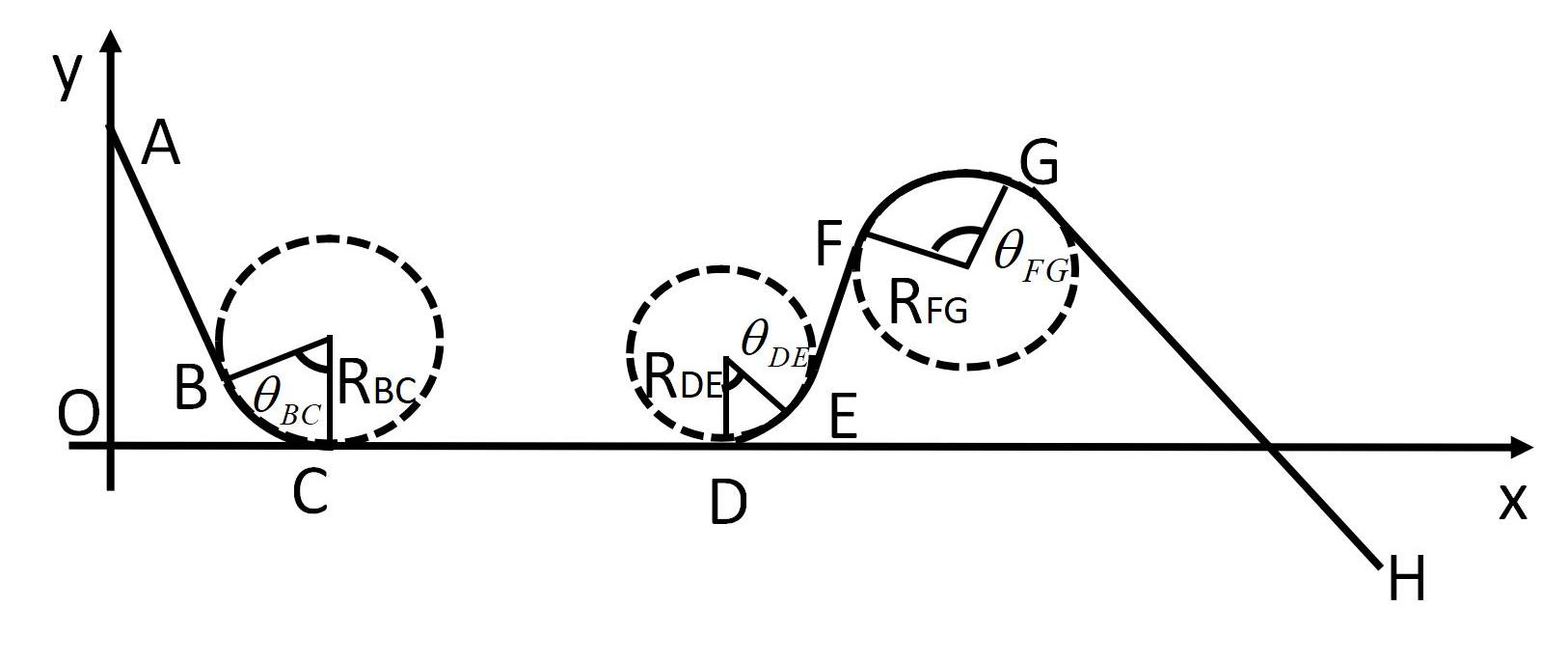
As for the maneuvering reference trajectory, an extensively used Dubins trajectory is selected as the planning path, shown in Fig. 3, where θjsubscript𝜃𝑗\theta_{j} (j=BC,DE,FG)𝑗𝐵𝐶𝐷𝐸𝐹𝐺(j=BC,DE,FG) and Rjsubscript𝑅𝑗R_{j} are the turning radius and central angles, respectively. The coordinates of the starting point, turning points and end point are A(0,450)𝐴0450A\left({0,450}\right), B(12000,50)𝐵1200050B\left({12000,50}\right), C(15000,0)𝐶150000C\left({15000,0}\right), D(24000,0)𝐷240000D\left({24000,0}\right), E(27000,50)𝐸2700050E\left({27000,50}\right), F(30000,150)𝐹30000150F\left({30000,150}\right), G(35000,260)𝐺35000260G\left({35000,260}\right) and H(48530,200)𝐻48530200H\left({48530,-200}\right). The time consumed per period is calculated by ti=l¯iVsubscript𝑡𝑖subscript¯𝑙𝑖𝑉{t_{i}}=\frac{{{{\bar{l}}_{i}}}}{V} (i=AB,CD,EF,GH)𝑖𝐴𝐵𝐶𝐷𝐸𝐹𝐺𝐻\left({i=AB,CD,EF,GH}\right) through straight regions and tj=ljV=θjRjVsubscript𝑡𝑗subscriptl𝑗𝑉subscript𝜃𝑗subscript𝑅𝑗𝑉{t_{j}}=\frac{{{{\mathord{\buildrel{\lower 3.0pt\hbox{$\scriptscriptstyle\frown$}}\over{l}}}_{j}}}}{V}=\frac{{{\theta_{j}}{R_{j}}}}{V} (j=BC,DE,FG)𝑗𝐵𝐶𝐷𝐸𝐹𝐺\left({j=BC,DE,FG}\right) in turning areas. Since the proposed performance funnel is time-triggered based on the planning path, the triggered times are set in accordance with the time points of the reference trajectory, resulting in p=3𝑝3p=3. Thus the parameters of the funnel boundary function of the form (2.2) are chosen as in Table 2.
Refer to caption
Figure 3: Planning trajectory for RV

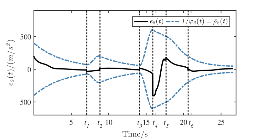
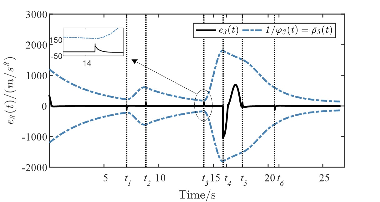
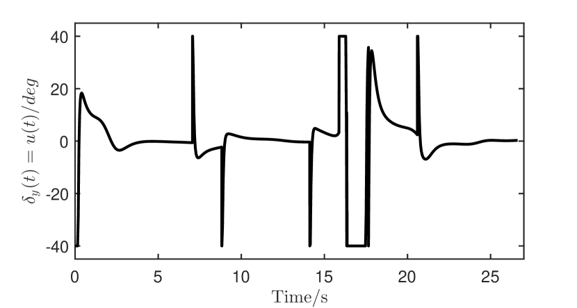
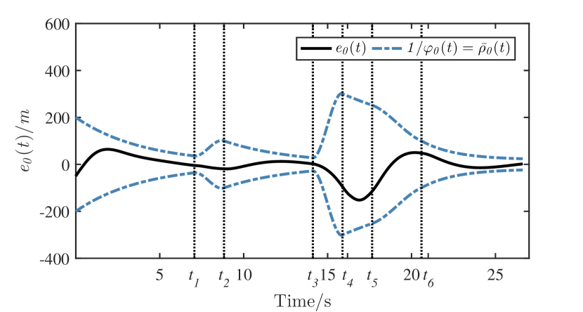
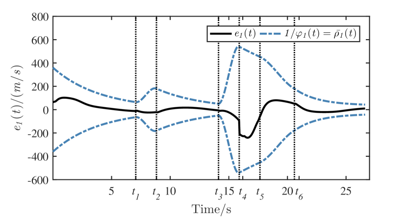
The simulation is depicted in Figs. 410. The tracking error e0subscript𝑒0e_{0} and the auxiliary errors e1,e2,e3subscript𝑒1subscript𝑒2subscript𝑒3e_{1},e_{2},e_{3} are shown in Figs. 47. It is found that e3subscript𝑒3e_{3} is more sensitive to maneuvering than e0subscript𝑒0e_{0}, where a slight jump appears near each trigger time. Every error eisubscript𝑒𝑖e_{i} (i=0,1,2,3)𝑖0123(i=0,1,2,3) is kept within its respective funnel through the whole process and under the influence of disturbances. The control input, namely the rudder angle, is shown in Fig. 8. It can be seen that the control input reaches saturation due to the input constraints. Although the saturation is not covered by Theorem 1, the controller obviously exhibits an exceptional performance under input constraints. Further research is necessary to find theoretical guarantees for this performance.

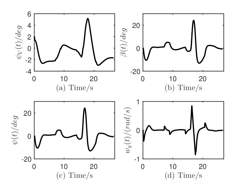
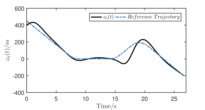
Fig. 9 shows the deflection angle, sideslip angle, yaw angle and yaw rate to illustrate that all variables in the closed-loop system are bounded. The tracking maneuver reference trajectory is shown in Fig. 10 together with the output signal generated under control. Although the performance of the vehicle in the continuous large maneuver segment is not as good as that in the single maneuver segment, we observe a decent tracking performance overall.

However, we like to note that in this example the theoretical condition (31) from Theorem 1 is not satisfied, yet the controller still works. This shows that the assumptions of Theorem 1 are quite conservative and further research is necessary to relax them. A thorough inspection of the proof of Theorem 1 reveals that the conservativeness of condition (31) is due to the utilization of the mean value theorem and avoiding it could lead to a weaker condition.
Refer to caption
Figure 4: Response of tracking error e0(t)subscript𝑒0𝑡e_{0}(t).
Refer to caption
Figure 5: Response of error e1(t)subscript𝑒1𝑡e_{1}(t).
Refer to caption
Figure 6: Response of error e2(t)subscript𝑒2𝑡e_{2}(t).
Refer to caption
Figure 7: Response of error e3(t)subscript𝑒3𝑡e_{3}(t).
Refer to caption
Figure 8: Response of control input δy(t)=u(t)subscript𝛿𝑦𝑡𝑢𝑡\delta_{y}(t)=u(t).
Refer to caption
Figure 9: Response of system: (a) ψV(t)subscript𝜓𝑉𝑡\psi_{V}(t), (b) β(t)𝛽𝑡\beta(t), (c) ψ(t)𝜓𝑡\psi(t), (d) ωy(t)subscript𝜔𝑦𝑡\omega_{y}(t).
Refer to caption
Figure 10: Tracking response of flight altitude zhsubscript𝑧z_{h}.
Table 1: Geometric parameters and initial state of RV
Variables Value Variables Value
m (kg) 1200 zh(0)subscript𝑧0z_{h}(0) (m) 400
S (m2superscriptm2\rm{m^{2}}) 1.3 ψV(0)subscript𝜓𝑉0\psi_{V}(0) (rad) 2/57.3
l𝑙l (m) 1.7 ψ(0)𝜓0\psi(0) (rad) 4/57.3
Jysubscript𝐽𝑦J_{y} (kgm2)kgsuperscriptm2({\rm{kg}}\cdot{{\rm{m}}^{2}}) 8110 ωy(0)subscript𝜔𝑦0\omega_{y}(0) (rad/s) 0.035
α𝛼\alpha (rad) 5/57.3 β(0)𝛽0\beta(0) 2/57.3
czαsuperscriptsubscript𝑐𝑧𝛼c_{z}^{\alpha} 0 czβsuperscriptsubscript𝑐𝑧𝛽c_{z}^{\beta} 0.1852
cz0superscriptsubscript𝑐𝑧0c_{z}^{0} -0.018714 cMαsuperscriptsubscript𝑐𝑀𝛼c_{M}^{\alpha} -0.1
cMβsuperscriptsubscript𝑐𝑀𝛽c_{M}^{\beta} 2.1335 cMδysuperscriptsubscript𝑐𝑀subscript𝛿𝑦c_{M}^{\delta_{y}} 5.1588
cM0superscriptsubscript𝑐𝑀0c_{M}^{0} 0.18979 q¯¯𝑞\bar{q} 3711.93329
Table 2: Parameters of the proposed funnel boundary
Variables Value
ρ¯0(t)subscript¯𝜌0𝑡\bar{\rho}_{0}(t) ρ¯0,10=200superscriptsubscript¯𝜌010200\bar{\rho}_{0,1}^{0}={\rm{200}}, ρ¯0,20=100superscriptsubscript¯𝜌020100\bar{\rho}_{0,2}^{0}=100, ρ¯0,30=300superscriptsubscript¯𝜌030300\bar{\rho}_{0,3}^{0}=300, ρ¯0,40=100superscriptsubscript¯𝜌040100\bar{\rho}_{0,4}^{0}=100, ρ¯0,1=2superscriptsubscript¯𝜌012\bar{\rho}_{0,1}^{\infty}=2, ρ¯0,2=2superscriptsubscript¯𝜌022\bar{\rho}_{0,2}^{\infty}=2, ρ¯0,3=2superscriptsubscript¯𝜌032\bar{\rho}_{0,3}^{\infty}=2, ρ¯0,4=10superscriptsubscript¯𝜌0410\bar{\rho}_{0,4}^{\infty}=10, l0,1=0.25subscript𝑙010.25{l_{0,1}}=0.25, l0,2=0.25subscript𝑙020.25{l_{0,2}}=0.25, l0,3=0.5,l0,4=0.1formulae-sequencesubscript𝑙030.5subscript𝑙040.1{l_{0,3}}=0.5,{l_{0,4}}=0.1
ρ¯i(t)subscript¯𝜌𝑖𝑡\bar{\rho}_{i}(t) (i=1,2,3)𝑖123(i=1,2,3) ρ¯1(t)=1.8ρ¯0(t)subscript¯𝜌1𝑡1.8subscript¯𝜌0𝑡{{\bar{\rho}}_{1}}\left(t\right)=1.8{{\bar{\rho}}_{0}}\left(t\right), ρ¯2(t)=2ρ¯0(t)subscript¯𝜌2𝑡2subscript¯𝜌0𝑡{{\bar{\rho}}_{2}}\left(t\right)=2{{\bar{\rho}}_{0}}\left(t\right), ρ¯3(t)=6ρ¯0(t)subscript¯𝜌3𝑡6subscript¯𝜌0𝑡{{\bar{\rho}}_{3}}\left(t\right)=6{{\bar{\rho}}_{0}}\left(t\right)

5 CONCLUSION

In this paper, we proposed a novel funnel-based tracking control algorithm for guaranteeing prescribed performance of the tracking error in reentry vehicle maneuvering flight. A time triggered non-monotonic funnel boundary is designed to successfully improve the controller performance, which is verified by simulations. The results show that the proposed control method has the ability to stabilize the closed-loop system under arbitrary bounded disturbances. Future research will focus on the relaxation of the conditions of Theorem 1 as well as their extension to the presence of input constraints. To this end, the recent results in [30] might be a starting point.

References

  • [1] Han T, Hu Q, Shin H S, et al. Incremental twisting fault tolerant control for hypersonic vehicles with partial model knowledge. IEEE Transactions on Industrial Informatics, 2021, 18(2): 1050-1060.
  • [2] Chai R, Tsourdos A, Savvaris A L, et al. Trajectory planning for hypersonic reentry vehicle satisfying deterministic and probabilistic constraints. Acta Astronautica, 2020, 177: 30-38.
  • [3] Shen G, Xia Y, Zhang J, et al. Adaptive super-twisting sliding mode altitude trajectory tracking control for reentry vehicle. ISA transactions, 2022.
  • [4] Mehra R. A comparison of several nonlinear filters for reentry vehicle tracking. IEEE Transactions on Automatic Control 1971, 16(4):307-319.
  • [5] Peng Z, Wang D, Li T, et al. Output-feedback cooperative formation maneuvering of autonomous surface vehicles with connectivity preservation and collision avoidance. IEEE Transactions on Cybernetics, 2019, 50(6): 2527-2535.
  • [6] Yao P, Wang H, Su Z. Real-time path planning of unmanned aerial vehicle for target tracking and obstacle avoidance in complex dynamic environment. Aerospace Science and Technology, 2015, 47: 269-279.
  • [7] Zhang R, Zong Q, Zhang X, et al. Game of Drones: Multi-UAV Pursuit-Evasion Game With Online Motion Planning by Deep Reinforcement Learning. IEEE Transactions on Neural Networks and Learning Systems, 2022.
  • [8] Yang H I, Zhao Y J. Trajectory planning for autonomous aerospace vehicles amid known obstacles and conflicts. J. Guid. Control Dyn, 2004, 27 (6): 997–1008.
  • [9] Pounds P E, Bersak D R, Dollar A M. Stability of small-scale UAV helicopters and quadrotors with added payload mass under PID control. Auton. Robots, 2012, 129–142.
  • [10] Elmokadem T, Zribi M, Youcef-Toumi K. Trajectory tracking sliding mode control of underactuated AUVs. Nonlinear Dynamics, 2016, 84(2): 1079-1091.
  • [11] Cho G R, Li J H, Park D, et al. Robust trajectory tracking of autonomous underwater vehicles using back-stepping control and time delay estimation. Ocean Engineering, 2020, 201: 107131.
  • [12] Beikzadeh H, Liu G. Trajectory tracking of quadrotor flying manipulators using L1 adaptive control. Journal of the Franklin Institute, 2018, 355(14): 6239-6261.
  • [13] Zuo Z, Ru P. Augmented L-1 adaptive tracking control of quad-rotor unmanned aircrafts. IEEE Trans. Aerosp. Electron. Syst, 2014, 50 (4): 3090–3101 .
  • [14] Mu C, Ni Z, Sun C, et al. Air-breathing hypersonic vehicle tracking control based on adaptive dynamic programming. IEEE transactions on neural networks and learning systems, 2016, 28(3): 584-598.
  • [15] Peng Z, Wang J. Output-feedback path-following control of autonomous underwater vehicles based on an extended state observer and projection neural networks. IEEE Transactions on Systems, Man, and Cybernetics: Systems, 2017, 48(4): 535-544.
  • [16] Bechlioulis C P, Rovithakis G A. Robust adaptive control of feedback linearizable MIMO nonlinear systems with prescribed performance. IEEE Transactions on Automatic Control, 2008, 53(9): 2090-2099.
  • [17] Bechlioulis C P, Rovithakis G A. Adaptive control with guaranteed transient and steady state tracking error bounds for strict feedback systems. Automatica, 2009, 45(2): 532-538.
  • [18] Bechlioulis C P, Rovithakis G A. A low-complexity global approximation-free control scheme with prescribed performance for unknown pure feedback systems. Automatica, 2014, 50(4): 1217-1226.
  • [19] Ilchmann A, Ryan E P, Sangwin C J. Tracking with prescribed transient behaviour. ESAIM: Control, Optimisation and Calculus of Variations, 2002, 7: 471-493.
  • [20] Berger T, Lê H H, Reis T. Funnel control for nonlinear systems with known strict relative degree. Automatica, 2018, 87: 345-357.
  • [21] Berger T, Ilchmann A, Ryan E P. Funnel control of nonlinear systems. Mathematics of Control, Signals, and Systems, 2021, 33: 151-194.
  • [22] Berger T, Rauert A L. Funnel cruise control. Automatica, 2020, 119: 109061.
  • [23] Berger T, Puche M, Schwenninger F L. Funnel control for a moving water tank. Automatica, 2022, 135: 109999.
  • [24] Gu X, Guo J, Guo Z, et al. Performance improvement-oriented reentry attitude control for reusable launch vehicles with overload constraint. ISA transactions, 2022, 128: 386-396.
  • [25] Bu X. Guaranteeing prescribed performance for air-breathing hypersonic vehicles via an adaptive non-affine tracking controller. Acta Astronautica, 2018, 151: 368-379.
  • [26] Bu X, Wei D, Wu X, et al. Guaranteeing preselected tracking quality for air-breathing hypersonic non-affine models with an unknown control direction via concise neural control. Journal of the Franklin Institute, 2016, 353(13): 3207-3232.
  • [27] Chai R, Tsourdos A, Savvaris A L, et al. Trajectory planning for hypersonic reentry vehicle satisfying deterministic and probabilistic constraints. Acta Astronautica, 2020, 177: 30-38.
  • [28] Hu G, Guo J, Guo Z, et al. ADP-based intelligent tracking algorithm for reentry vehicles subjected to model and state uncertainties. IEEE Transactions on Industrial Informatics, 2022.
  • [29] Ilchmann A, Ryan E P. Performance funnels and tracking control. International Journal of Control, 2009, 82(10): 1828-1840.
  • [30] Berger T. Input-constrained funnel control of nonlinear systems. Submitted for publication, preprint available on arXiv: https://arxiv.org/abs/2202.05494.