Orbital-free Density Functional Theory: differences and similarities between electronic and nuclear systems

Abstract

Orbital-free Density Functional Theory (OF-DFT) has been used when studying atoms, molecules and solids. In nuclear physics, there has been basically no application of OF-DFT so far, as the Density Functional Theory (DFT) has been widely applied to the study of many nuclear properties mostly within the Kohn-Sham (KS) scheme. There are many realizations of nuclear KS-DFT, but computations become very demanding for heavy systems, such as superheavy nuclei and the inner crust of neutron stars, and it is hard to describe exotic nuclear shapes using a finite basis made with a limited number of orbitals. These bottlenecks could, in principle, be overcome by an orbital-free formulation of DFT. This work is a first step towards the application of OF-DFT to nuclei. In particular, we have implemented possible choices for an orbital-free kinetic energy and solved the associated Schrödinger equation either with simple potentials or with simplified nuclear density functionals. While the former choice sheds light on the differences between electronic and nuclear systems, the latter choice allows us discussing the practical applications to nuclei and the open questions.

Density Functional Theory, Nuclear physics, Nuclear ground-state properties, Thomas-Fermi approximation

1 Introduction

Orbital-free Density Functional Theory (OF-DFT) has been introduced in Ref. PhysRevA.30.2745 , in which an interestng remark was introduced, related to the original Hohenberg-Kohn (HK) theorem HK.64 . This HK theorem sets an exact one-to-one correspondence between the energy $E$ of an interacting fermion system and that of a fictitious, non-interacting fermion systems ($E_{\rm f}$) with the same density $\rho$. If $\rho$ is, in turn, expressed in terms of orbitals like $\rho=\sum_{j}|\phi_{j}|^{2}$ we have the usual Kohn-Sham (KS) formulation of DFT KS.65 . The Kohn-Sham form of the Energy Density Functional (EDF) is

$$E_{\rm f}=E_{\rm KS}=\sum_{j}\int d^{3}r\ \phi_{j}^{*}(\mbox{\boldmath$r$})\left(-\frac{\hbar^{2}}{2m}\nabla^{2}\right)\phi_{j}(\mbox{\boldmath$r$})+\int d^{3}r\ {\cal V}_{\rm KS}[\rho],$$ (1)

where the first term is the kinetic energy with a mass $m$ and the second term includes all interactions (for electronic systems, this means Hartree energy, exchange-correlation energy, and interaction with the external potential).

In Ref. PhysRevA.30.2745 , the authors have noted that one can actually map the interacting fermion system onto a non-interacting boson system. In fact, in the proof of the HK theorem, no special role is played by the statistics of the particles (as well as by their mass). Therefore, one could write the energy of the system as

$$E_{\rm b}=E_{\rm OF-DFT}=\frac{\hbar^{2}}{2m}\ \int d^{3}r\ \left(\mbox{\boldmath$\nabla$}\sqrt{\rho}\right)^{2}+\int d^{3}r\ {\cal V}[\rho],$$ (2)

where now the first term is the boson kinetic energy. The second term could be, at least in principle, related to the KS interaction energy by adding the KS kinetic energy and subtracting the boson kinetic energy (one should remember here that the KS kinetic energy, although written in terms of orbitals, must be a functional of $\rho$ as every property of the system at hand is).

Either from Eq. (1) or (2), one can minimize the energy using the variational principle with a fixed number or particles. From Eq. (1) one easily obtains the famous Kohn-Sham set of equations,

$$\left(-\frac{\hbar^{2}}{2m}\nabla^{2}+v_{KS}\right)\phi_{j}(\mbox{\boldmath$r$})=\varepsilon_{j}\phi_{j}(\mbox{\boldmath$r$}),$$ (3)

where the effective KS potential is $v_{KS}\equiv\frac{\delta}{\delta\rho}\int d^{3}r\ {\cal V}[\rho]=\frac{\partial{\cal V}}{\partial\rho}$ and $\varepsilon_{j}$ are the Lagrange multipliers associated with the normalisation of the single orbitals, that are interpreted as eigenenergies of those orbitals. On the other hand, if one starts from Eq. (2) and applies

$$\frac{\delta}{\delta\rho}\left(E-\mu\int d^{3}r\ \rho\right)=0,$$ (4)

one easily arrives at

$$\left(-\frac{\hbar^{2}}{2m}\nabla^{2}+\frac{\partial{\cal V}}{\partial\rho}\right)\sqrt{\rho}=\mu\sqrt{\rho},$$ (5)

which is the basic (Euler) equation of OF-DFT. We shall simply write $v=\frac{\partial{\cal V}}{\partial\rho}$ in what follows.

The practical advantage of the latter Eq. (5) over the conventional KS equations (3) is clear. Instead of solving $N$ equations for $N$ orbitals, one has to solve only one equation. All particles lie on a single orbital and this must have a simple shape, like that of a $\ell=0$ orbital in a spherical potential etc. This has motivated a series of applications for atoms, molecules and solids; useful papers that review many of these applications are, e.g., Chen2008 ; Karasiev2012 ; Witt2018 . Even public software is available Golub2020 . The time-dependent (TD) extension of OF-DFT is discussed in Ref. Pavanello2021 and references therein.

In the case of nuclear systems, the advantages brought by OF-DFT can be even stronger. Many finite nuclei have intrinsic deformed shapes, so that Kohn-Sham levels have little degeneracy and the set of equations can be very large. Super-heavy nuclei, or nucleons in the inner crust of neutron stars, are still a big challenge for conventional nuclear DFT and the same can be said for time-dependent calculations. OF-DFT can be very instrumental in all these cases and not only. Some nuclei are known to exhibit shape coexistence, and a description in terms of orbitals calls for a superposition of orbitals associated with different shapes, that are non-orthogonal. A prospective OF-DFT description would be simpler to implement and to interpret.

Despite these motivations, to the best of our knowledge the only mention of nuclear OF-DFT is in Ref. Bulgac2018 , where an orbital-free formulation is proposed as an alternative to KS for the global fit of masses but no details are provided. Therefore, our purpose in the present work is to start to fill this gap. In particular, the scope of the paper is to explore different prescriptions for the orbital-free kinetic energy, and see how they perform for simple nuclei. One of the key questions that we have in mind is if there are basic differences between electronic and nuclear systems due to the long-range or short-range character of the underlying interaction. Ultimately, we would like to assess to which extent OF-DFT is useful for nuclear systems.

Notice that OF-DFT bears some resemblance with what has been called in the nuclear physics context as Thomas-Fermi (TF) approximation or extended TF (ETF) Brack1985 ; Centelles1990 ; ETFSI1986 ; ETFSI1987 ; ETFSI1991 ; ETFSI1992 ; ETFSI2001 . In Ref. Brack1985 , it was demonstrated that the ETF approximation provides a good description of the ground state energy but it yields a wrong tail of the density distribution (see also Ref. Bohigas1976 ). A simple recipe was considered in Ref. Brack1985 to cure this problem by changing the coefficient of the Weizäcker correction term in the kinetic energy in the ETF approximation. In this paper, we also address the question on the density distributions and the capability of OF-DFT to reproduce its asymptotic tail.

The paper is organized as follows. In Section 2, some possible choices of the OF-DFT ansatz, together with the relationship with ETF, are discussed. In Section 3, we present our first, exporatory results aimed at showing analogies and differences between nuclear and Coulomb systems. In Section 4, we move to applications based on a realistic albeit simplified nuclear interaction and we discuss the issue of the shell structure. Our conclusions are drawn in Section 5.

2 The OF-DFT kinetic energy

We go back to Eq. (2), that is,

$$E=\frac{\hbar^{2}}{2m}\ \int d^{3}r\ \left(\mbox{\boldmath$\nabla$}\sqrt{\rho}\right)^{2}+\int d^{3}r\ {\cal V}[\rho]\equiv T+V.$$

Let us assume we have an ansatz for $V$ and let us focus on how to start from the boson kinetic energy $T$ and approximate the fermion kinetic energy at best, keeping a density-dependent (and not orbital-dependent) form.

The mere replacement of the fermion kinetic energy with the boson one is named after Von Weiszäcker (vW). In this case,

$$T=T_{\rm vW}\equiv\frac{\hbar^{2}}{2m}\ \int d^{3}r\ \left(\mbox{\boldmath$\nabla$}\sqrt{\rho}\right)^{2}.$$ (6)

This expression is obviously exact for a single fermion, or two fermions in a spin-singlet state. In Coulomb systems, it provides a rigorous lower bound to the exact kinetic energy (cf. Sec. 1a of Ref. Witt2018 ). A sort of complementary choice is the kinetic energy given by the TF approximation, that takes care of the Pauli principle and is exact in a uniform system, but is approximate for finite systems. In this case,

$$T_{\rm TF}=\frac{\hbar^{2}}{2m}\ \int d^{3}r\ \frac{3}{5}\left(3\pi^{2}\right)^{2/3}\rho^{5/3}.$$ (7)

This form of the kinetic energy is close to another rigorous lower bound, as shown by E. Lieb RevModPhys.48.553 . The TF approximation is known to have shortcomings in the nuclear case, and in particular not to provide the correct asymptotic form of the nuclear densities Brack1985 ; Centelles1990 .

In the Coulomb case, there exist some pragmatic prescriptions to mix vW and TF. One possibility is

$$T_{\rm{TF},{\rm vW},\beta}=T_{\rm TF}+\beta T_{\rm vW},$$ (8)

even though one may also introduce another factor in front of the first term. This equation is motivated by a conjecture, again by E. Lieb Lieb1979 , namely that the exact kinetic energy $T$ should obey $T<T_{\rm vW}+T_{TF}$. Popular choices for $\beta$ are $\beta=\frac{1}{5}$ and $\frac{1}{9}$. One could use the response function of the uniform free electron gas $\chi_{0}$ and write the kinetic energy of the slightly perturbed gas: the second order expansion in $\nabla\rho$ is equivalent to $\beta=\frac{1}{9}$ in Eq. (8). The choice of $\beta=\frac{1}{9}$ can also be obtained with the semi-classical approximation to the kinetic energy, while $\beta=1$ is the original value derived by Weizäcker. $\beta=\frac{1}{5}$ was obtained from empirical fits.

Another possible choice is

$$T=\int d^{3}r\ \tau_{\rm TF}\ F(\mbox{\boldmath$r$}),$$ (9)

where $F$ is the so-called enhancement factor. We mention this choice because it has been adopted in Ref. Bulgac2018 ; the corresponding expression of $F$ is provided in the Appendix of this paper. We have tested this choice, and checked that we obtain results that lead to the same qualitative conclusions obtained with our simpler prescription (8). Notice that if one adopts

$$F=\left(1+\beta\frac{\tau_{\rm vW}}{\tau_{\rm TF}}\right),$$ (10)

then one goes back to Eq. (8).

In what follows, we are going to display results obtained by solving the Euler equation (5) in spherical symmetry. The explicit form of the equation in this case is provided in the Appendix.

3 Results for simple potential models

In this section, we use simple systems of non-interacting Fermions in a given potential. The model Hamiltonian for such systems reads

$$H=\sum_{i}\left(-\frac{\hbar^{2}}{2m}\mbox{\boldmath$\nabla$}_{i}^{2}+V(\mbox{\boldmath$r$}_{i})\right).$$ (11)

The total energy for this Hamiltonian is obviously,

$$E=\sum_{i:{\rm occ}}\epsilon_{i}$$ (12)

that is, the sum of the eigenenergies for the occupied orbits.

3.1 Nuclear systems

Let us first consider a system with 8 neutrons in a Woods-Saxon potential given by

$$V(r)=-\frac{V_{0}}{1+\exp[(r-R_{0})/a]},$$ (13)

with $V_{0}=$ 50 MeV, $R_{0}=1.2\times 16^{1/3}$ fm, and $a=0.65$ fm, mimicking the ¹⁶O nucleus. For simplicity, the spin-orbit interaction is ignored. The single-particle energies $\epsilon$ with this potential are $-32.6$ MeV and $-16.8$ MeV for the 1s and 1p states, respectively.

Table 1: Values of the total energy and of the r.m.s. radius of ¹⁶O, calculated either with the potential (13) (this result is labelled as exact) or with different prescriptions for the kinetic energy as defined by Eq. (8).

	$E$ (MeV)	$\sqrt{\langle r^{2}\rangle}$ (fm)
exact	$-142.27$	2.575
OF-DFT ($\beta=1/9$)	$-140.85$	2.500
OF-DFT ($\beta=1/5$)	$-135.19$	2.562
OF-DFT ($\beta=1$)	$-96.31$	3.12

The total energies and the root-mean-square radii for several values of $\beta$ are summarized in Table 1. The corresponding density distributions are shown in Fig. 1. These results indicate that $\beta=1/9$ is slightly better for the total energy while $\beta=1/5$ is slightly better for the r.m.s. radius. Both choices can be reasonable although not highly accurate, while $\beta=1$ should be discarded. This overall conclusion is confirmed by looking at the density distributions. In particular, the exponential tail shown in the middle panel indicates that the tail is not well reproduced with $\beta=1/9$ and $\beta=1$ as has been discussed in Ref. Brack1985 , while $\beta=1/5$ significantly improves the tail. This consideration may be important when applying OF-DFT, e.g., to nuclear reactions.

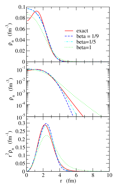
Figure 1: Density distributions as a function of the radius $r$ for a system with 8 neutrons in a Woods-Saxon potential given by Eq. (13). The top and the middle panels show the density distributions in the linear and in the logarithmic scales, respectively, while the bottom panel shows the densities in the linear scale multiplied by $r^{2}$. In each panel, the solid line denotes the exact density, while the dashed, the dot-dashed, and the dotted lines show the densities from the orbital-free DFT with $\beta$ = 1/5, 1/9, and 1, respectively.

3.2 Coulomb systems

We next consider a system of 10 electrons in the attractive Coulomb potential

$$V(r)=-\frac{10e^{2}}{r}.$$ (14)

We use atomic units in this subsection. The eigenenergies of this potential are $\epsilon=-50.0$ (Ha) for the 1S orbital and $-12.5$ (Ha) for the 2P and 2S orbitals. The results are shown in Table 2 and Fig. 2.

Table 2: Values of the total energy and of the r.m.s. radius of the 10 electrons bound by the Coulomb potential (14). The exact result is compared with different prescriptions for the kinetic energy as defined by Eq. (8).

method	$E$ (Ha)	$\sqrt{\langle r^{2}\rangle}$ (a.u.)
exact	$-200.0$	0.27
OF-DFT ($\beta=1/9$)	$-208.6$	0.30
OF-DFT ($\beta=1/5$)	$-196.1$	0.318
OF-DFT ($\beta=1$)	$-141.96$	0.482

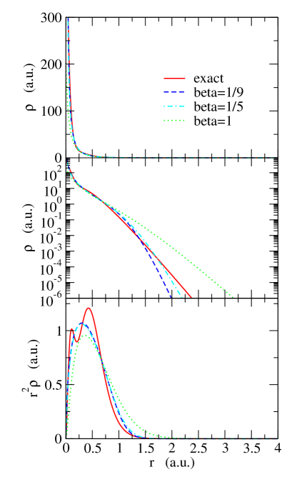
Figure 2: Same as Fig. 1, but for a system with 10 electrons in a Coulomb potential given by Eq. (14).

From Table 2, one can see that there is not a big difference between the results obtained with $\beta=1/5$ and $\beta=1/9$, while $\beta=1$ does not perform well, as it was the case for the nuclear system that we have just discussed. The same qualitative conclusion as in the nuclear case can be obtained for the tail of the density distributions: while the deviation is large for $\beta=1$ and 1/9, the choice of $\beta=1/5$ significantly improves the surface behavior of the density distribution. However, we notice that the central density is considerably larger in the Coulomb case, and the deviation of the tail appears only at much smaller densities (relative to the central density) as compared to the nuclear case. The wrong tail in the density distribution would thus be much less relevant here as compared with the nuclear case.

4 Towards realistic models

In a first attempt towards realistic nuclear OF-DFT calculations, we have solved the self-consistent equations associated with the potential part of a Skyrme EDF, for a few spherical nuclei. In fact, we have used the simple force introduced in Ref. Agrawal2005a , that is,

$$v_{NN}(\mbox{\boldmath$r$},\mbox{\boldmath$r$}^{\prime})=\left[t_{0}+\frac{t_{3}}{6}\rho\left(\frac{\mbox{\boldmath$r$}+\mbox{\boldmath$r$}^{\prime}}{2}\right)^{\alpha}\right]\delta(\mbox{\boldmath$r$}-\mbox{\boldmath$r$}^{\prime}),$$ (15)

with which the potential part of the energy functional in Eq. (1) reads

$${\cal V}_{\rm KS}[\rho]=\frac{3}{8}t_{0}\rho(\mbox{\boldmath$r$})^{2}+\frac{t_{3}}{16}\rho(\mbox{\boldmath$r$})^{\alpha+2}.$$ (16)

We have used the same values for the parameters, $t_{0},t_{3}$, and $\alpha$ as those in Ref. Agrawal2005a . This is a semi-realistic choice which is not as accurate as a standard, complete Skyrme EDF; still, we can learn about shell effects.

In fact, a criticism that has been raised against OF-DFT is that shell effects may be somehow missing. A discussion of shell effects, for the Coulomb case, can be found e.g. in Ref. Yannouleas2013 . Similar discussions can be found, for the nuclear case, in several ETF works. For instance, in the density distributions, oscillations associated with the occupancies of different orbitals do not show up, at least with simplified effective potentials. Ideally, the exact OF-DFT should reproduce the exact density, including the oscillations. This means that, most likely, the exact OF-EDF will include a potential with more, or higher-order, derivative terms than those we can build at present.

At the moment, we have not had yet built sophisticated new OF-EDFs and this is not doable within a short-range perspective. Even though the Strutinsky shell correction method can be applied to the ground state energies ETFSI1986 ; ETFSI1987 ; ETFSI1991 ; ETFSI1992 ; ETFSI2001 ; Yannouleas2013 , we would like to take into account the shell effect on the density distributions as well. For this purpose, we have found a simple prescription that allows recovering the shell-effects with little cost, on top of OF-DFT. As has been done in Ref. Zhou2006 for the Coulomb case and in Ref.Bohigas1976 for the nuclear case, we have implemented the following procedure. After arriving at a converged OF result, we have included the resultant effective potential into the Kohn-Sham equation and carried out just one further iteration.

The results of this procedure are shown in Fig. 3. It can be easily seen that just one iteration of the Kohn-Sham equations using the converged potential from the OF Euler equation is enough to produce density distributions that are similar to the ones obtained from the full iterative Kohn-Sham procedure. This holds true as far as we consider shell effects, that is, the oscillations in the inner region, but also as far as the tail is considered. In Fig. 3, we emphasize the two complementary aspects by displaying densities both in linear and logarithmic scales. Our conclusion is quite general and it is demonstrated by using two different nuclei and the two reasonable choices for $\beta$, namely $\beta=1/5$ and $\beta=1/9$.

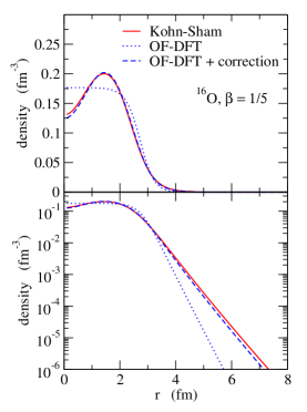
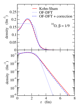
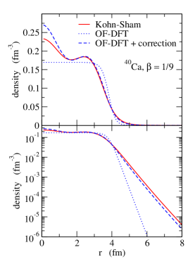
Figure 3: A comparison of the density distributions obtained with a simplified Skyrme EDF. The left, the middle, and the right panels show the density distributions for ¹⁶O from OF-DFT with $\beta=1/5$, those for ¹⁶O with $\beta=1/9$, and those for ⁴⁰Ca with $\beta=1/9$, respectively. The upper and the lower panels show the density distributions in the linear and the logarithmic scales, respectively. In each panel, the solid and the dotted lines show the density obtained with the Kohn-Sham method and the OF-DFT, respectively. The dashed lines show the densities with OF-DFT, but with the correction based on the last iteration using the Kohn-Sham method after the convergence is achieved with OF-DFT, as discussed in the text.

5 Conclusion

In this paper, we have made a first attempt to seriously answer the question if OF-DFT can be applied to nuclear systems with some chances of success. OF-DFT has been applied to Coulomb systems by different groups and in different ways. Nuclei are characterized by a different basic interaction, which is short-range rather than long-range; at the same time, nuclear DFT is more demanding from the computational viewpoint and the study of superheavy isotopes, or of the crust of neutron stars, would benefit from OF-DFT. Nuclei with shape coexistence, that are not easy to describe using a limited basis of single-particle orbitals, are a further motivation to explore OF-DFT for nuclei.

We have found that OF-DFT provides reasonable results for magic nuclei, once the kinetic energy has been approximated with Eq. (8) in a similar way as for electronic systems. A careful look into the density distributions reveals that the tails are not well reproduced both in the nuclear and the electronic cases, even though the long-range character of the Coulomb force does indeed play a role and washes out the discrepancies between the exact results and those with reasonable values of $\beta$, more than in the nuclear case. One of the interesting results of our work is that density distributions can be also markedly improved by just one last KS iteration, after the OF-DFT procedure has reached convergence.

Fine-tuning of the OF functionals is now in order. This is among our perspectives but, at the same time, one should develop the formalism to go beyond the simple EDFs that depend on the local number density only. OF versions of EDFs that depend on density gradients, higher-order derivatives or other generalized densities (spin-orbit densities, pairing densities etc.) should be investigated. We plan to go along this line, by comparing different formulations (for instance, spin polarization vs spin-orbit density). Another possible direction towards this goal may be to use deep learning techniques, as has been advocated in Ref. Hizawa2023 .

Last but not least, we should go beyond the spherical approximation and formulate OF-DFT for deformed nuclei. In this case, the way to optimize the energy may be re-discussed (see, e.g. Ref. Ryley2021 ). Moreover, it was argued in Ref. Brack1985 that the ETF approximation “fails to give reasonable deformation energies due to a drastic overestimation of the surface energy contributions” (see Sec. 3.3 in Ref. Brack1985 ). It would be interesting to see how well the deformation energy is described with the prescription of a singe KS iteration after convergence of OF-DFT.

More generally, past ETF studies of nuclear systems have not been able to go beyond some level of accuracy. The broad and novel perspective that we wish to highlight is going beyond ETF, with a more flexible form of the kinetic energy, and using state-of-the-art methods like Bayesian inference or machine learning Imoto2021 ; Zhao2022 to improve over ETF.

Appendix A Appendix: Euler equation and total energy in the spherical case

In this Appendix, we derive the Euler equation associated with the OF-DFT kinetic energy in the form of Eq. (8) and a generic potential part. We also specialize the result to the case of spherical symmetry.

The EDF with $T$ given by Eq. (8) reads

$$E=\beta\frac{\hbar^{2}}{2m}\ \int d^{3}r\ \left(\mbox{\boldmath$\nabla$}\sqrt{\rho}\right)^{2}+\alpha\frac{\hbar^{2}}{2m}\ \int d^{3}r\ \frac{3}{5}\left(3\pi^{2}\right)^{2/3}\rho^{5/3}+V[\rho].$$ (17)

The variation of the first term is

$$\frac{\delta T_{\rm vW}}{\delta\rho}=\frac{\partial\sqrt{\rho}}{\partial\rho}\frac{\delta T_{\rm vW}}{\delta\sqrt{\rho}}=\frac{1}{2\sqrt{\rho}}\left(-\mbox{\boldmath$\nabla$}\frac{\partial{\cal T}_{\rm vW}}{\partial\mbox{\boldmath$\nabla$}\rho}\right)=-\frac{\hbar^{2}}{2m}\frac{\nabla^{2}\sqrt{\rho}}{\sqrt{\rho}},$$ (18)

whereas, for the second term,

$$\frac{\delta T_{\rm TF}}{\delta\rho}=\frac{\hbar^{2}}{2m}\left(3\pi^{2}\right)^{2/3}\rho^{2/3}.$$ (19)

Then, the Euler equation becomes

$$\left[-\beta\frac{\hbar^{2}}{2m}\frac{\nabla^{2}\sqrt{\rho}}{\sqrt{\rho}}+\alpha\frac{\hbar^{2}}{2m}\left(3\pi^{2}\right)^{2/3}\rho^{2/3}+\frac{\delta V}{\delta\rho}\right]=\mu.$$ (20)

By multiplying $\sqrt{\rho}/\beta$ on both sides of this equation, one obtains

$$\left[-\frac{\hbar^{2}}{2m}\nabla^{2}+\frac{\alpha}{\beta}\frac{\hbar^{2}}{2m}\left(3\pi^{2}\right)^{2/3}\rho^{2/3}+\frac{1}{\beta}\frac{\delta V}{\delta\rho}\right]\sqrt{\rho}=\frac{\mu}{\beta}\sqrt{\rho}.$$ (21)

In general, using a spherical basis we can write

$$\sqrt{\rho}\equiv\Phi=\sum_{lm}\frac{\phi_{lm}}{r}Y_{lm},$$ (22)

In the spherical case, only $\phi_{00}$ is to be considered. From the previous equation (21) we easily obtain the reduced Schrödinger equation in the form

$$\left[-\frac{\hbar^{2}}{2m}\frac{d^{2}}{dr^{2}}+\frac{\hbar^{2}}{2m}\frac{l(l+1)}{r^{2}}+\frac{\alpha}{\beta}\frac{\hbar^{2}}{2m}\left(3\pi^{2}\right)^{2/3}\rho^{2/3}+\frac{1}{\beta}\frac{\delta V}{\delta\rho}\right]\phi=\frac{\mu}{\beta}\phi.$$ (23)

The total energy can be written in a useful form by exploiting the fact that

$$\mbox{\boldmath$\nabla$}\sqrt{\rho}=\frac{1}{2\sqrt{\rho}}\mbox{\boldmath$\nabla$}\rho=\frac{1}{2\rho}\frac{\partial\rho}{\partial r}\mbox{\boldmath$e$}_{r}.$$

In this way,

$$E = \beta\frac{\hbar^{2}}{2m}\ \int d^{3}r\ \frac{1}{4\rho}\left(\frac{\partial\rho}{\partial r}\right)^{2}+\alpha\frac{\hbar^{2}}{2m}\ \int d^{3}r\ \frac{3}{5}\left(3\pi^{2}\right)^{2/3}\rho^{5/3}+\int d^{3}r\ \frac{\delta V}{\delta\rho}\rho$$

$$= \beta\frac{\hbar^{2}}{2m}\ \int dr\ 4\pi r^{2}\frac{1}{4\rho}\left(\frac{\partial\rho}{\partial r}\right)^{2}+\alpha\frac{\hbar^{2}}{2m}\ \int dr\ 4\pi r^{2}\frac{3}{5}\left(3\pi^{2}\right)^{2/3}\rho^{5/3}+\int dr\ 4\pi r^{2}\frac{\delta V}{\delta\rho}\rho.$$

For the sake of completeness, we also report here the Euler equation and its reduction to the spherical case, in the specific case of the kinetic energy given by Eq. (9) with the enhancement factor proposed in Ref. Bulgac2018 , namely

$$F=\frac{1+\left(1+\kappa\right)X+9\kappa X^{2}}{1+\kappa X}$$ (25)

and

$$X=\frac{5}{27}\frac{|\nabla\sqrt{\rho}|^{2}}{\left(3\pi^{2}\right)^{2/3}\rho^{5/3}}.$$ (26)

In this case, the Euler equation becomes

$$\left[-\frac{\hbar^{2}}{2m}\frac{F^{\prime}}{9}\nabla^{2}+\frac{\hbar^{2}}{2m}\left(3\pi^{2}\right)^{2/3}\rho^{2/3}\left(F-F^{\prime}X\right)+\frac{\delta V}{\delta\rho}\right]\sqrt{\rho}=\mu\sqrt{\rho}.$$ (27)

In the spherical case, we easily arrive at

$$\frac{d^{2}\phi}{dr^{2}}=\left[\left(3\pi^{2}\right)^{2/3}\rho^{2/3}\frac{9\left(F-F^{\prime}X\right)}{F^{\prime}}+\frac{2m}{\hbar^{2}}\frac{9}{F^{\prime}}\frac{\delta V}{\delta\rho}-\frac{2m}{\hbar^{2}}\frac{9}{F^{\prime}}\mu\right]\phi.$$ (28)

The total energy reads

$$E=\frac{\hbar^{2}}{2m}\ \int d^{3}r\ \frac{3}{5}\left(3\pi^{2}\right)^{2/3}\rho^{5/3}F+\int d^{3}r\ \frac{\delta V}{\delta\rho}\rho$$ (29)

and we could also write

$$E=\mu-\frac{2}{5}\frac{\hbar^{2}}{2m}\ \int d^{3}r\left(F-F^{\prime}X\right)\left(3\pi^{2}\right)^{2/3}\rho^{5/3}.$$ (30)

The second term can be interpreted as a rearrangement energy.

References

- (1) Mel Levy, John P. Perdew, and Viraht Sahni, Phys. Rev. A, 30, 2745–2748 (Nov 1984).
- (2) P. Hohenberg and W. Kohn, Phys. Rev., 136, B864–B871 (1964).
- (3) W. Kohn and L. J. Sham, Phys. Rev., 140, A1133–A1138 (Nov 1965).
- (4) Huajie Chen and Aihui Zhou, Numer. Math. Theory, Methods Appl., 1(1), 1–28 (2008).
- (5) V. V. Karasiev and S. B. Trickey, Comput. Phys. Commun., 183(12), 2519–2527 (dec 2012), 1109.6602.
- (6) William C. Witt, Beatriz G. Del Rio, Johannes M. Dieterich, and Emily A. Carter, J. Mater. Res. 2017 337, 33(7), 777–795 (apr 2018).
- (7) Pavlo Golub and Sergei Manzhos, Computer Physics Communications, 256, 107365 (2020).
- (8) Kaili Jiang and Michele Pavanello, Phys. Rev. B, 103, 245102 (Jun 2021).
- (9) Aurel Bulgac, Michael Mc Neil Forbes, Shi Jin, Rodrigo Navarro Perez, and Nicolas Schunck, Phys. Rev. C, 97(4), 044313 (apr 2018), 1708.08771.
- (10) M Brack, C Guet, and H.-B Håkansson, Physics Reports, 123(5), 275–364 (1985).
- (11) M. Centelles, M. Pi, X. Viñas, F. Garcias, and M. Barranco, Nucl. Phys. A, 510(3), 397–416 (apr 1990).
- (12) A.K. Dutta, J.-P. Arcoragi, J.M. Pearson, R. Behrman, and F. Tondeur, Nuclear Physics A, 458(1), 77–94 (1986).
- (13) F. Tondeur, A.K. Dutta, J.M. Pearson, and R. Behrman, Nuclear Physics A, 470(1), 93–106 (1987).
- (14) J.M. Pearson, Y. Aboussir, A.K. Dutta, R.C. Nayak, M. Farine, and F. Tondeur, Nuclear Physics A, 528(1), 1–47 (1991).
- (15) Y. Aboussir, J.M. Pearson, A.K. Dutta, and F. Tondeur, Nuclear Physics A, 549(2), 155–179 (1992).
- (16) A. Mamdouh, J.M. Pearson, M. Rayet, and F. Tondeur, Nuclear Physics A, 679(3), 337–358 (2001).
- (17) O. Bohigas, X. Campi, H. Krivine, and J. Treiner, Physics Letters B, 64(4), 381–385 (1976).
- (18) Elliott H. Lieb, Rev. Mod. Phys., 48, 553–569 (Oct 1976).
- (19) Elliott Lieb, In Konrad Osterwalder, editor, Mathematical Problems in Theoretical Physics, page … Springer, Berlin-Heidelberg-New York (1980).
- (20) B K Agrawal, S Shlomo, and V Kim Au, Phys. Rev. C, 72, 14310 (2005).
- (21) Constantine Yannouleas and Uzi Landman, In Yan Alexander Wang and Tomasz Adam Wesolowski, editors, Recent Advances in Orbital-Free Density Functional Theory, page 203. World Scientific, Singapore (2013).
- (22) Baojing Zhou and Yan Alexander Wang, J. Chem. Phys., 124(8), 81107 (feb 2006).
- (23) N. Hizawa, K. Hagino, and K. Yoshida (2023), arXiv:2306.11314.
- (24) Matthew S. Ryley, Michael Withnall, Tom J. P. Irons, Trygve Helgaker, and Andrew M. Teale, The Journal of Physical Chemistry A, 125(1), 459–475, PMID: 33356245 (2021), https://doi.org/10.1021/acs.jpca.0c09502.
- (25) Fumihiro Imoto, Masatoshi Imada, and Atsushi Oshiyama, Phys. Rev. Res., 3, 033198 (Aug 2021).
- (26) X. H. Wu, Z. X. Ren, and P. W. Zhao, Phys. Rev. C, 105, L031303 (Mar 2022).