Deep Image Harmonization with Globally Guided Feature Transformation and Relation Distillation

Abstract

Given a composite image, image harmonization aims to adjust the foreground illumination to be consistent with background. Previous methods have explored transforming foreground features to achieve competitive performance. In this work, we show that using global information to guide foreground feature transformation could achieve significant improvement. Besides, we propose to transfer the foreground-background relation from real images to composite images, which can provide intermediate supervision for the transformed encoder features. Additionally, considering the drawbacks of existing harmonization datasets, we also contribute a ccHarmony dataset which simulates the natural illumination variation. Extensive experiments on iHarmony4 and our contributed dataset demonstrate the superiority of our method. Our ccHarmony dataset is released at https://github.com/bcmi/Image-Harmonization-Dataset-ccHarmony.

1 Introduction

Image composition [31, 6] is an essential editing operation to combine regions from different images to produce composite images, which has a variety of vision applications like advertisement propaganda and digital entertainment [34, 28]. Nevertheless, when pasting the foreground extracted from one image on another background image, the resultant composite image may have inconsistent illumination statistics. Image harmonization [10, 29] aims to adjust the foreground illumination for visual consistency within the composite image. In recent years, deep learning based image harmonization methods [10, 36, 18, 29, 20, 15] have sprouted out and achieved remarkable progress.

Existing methods [33, 49, 11, 34, 22] have developed myriads of techniques to address the mismatch between foreground and background illumination. Among them, some works [29, 11] revealed that specially transforming the foreground features can enhance the performance, since the main goal of image harmonization is adjusting the foreground. For example, [29, 17] transfer the feature statistics (e.g., mean, variance) from background to foreground. [11, 36] process foreground and background features separately using different channel attentions. These methods only leverage the information within the same feature map to transform the foreground features, lacking the guidance of global information. However, the global information of the whole composite image is very likely to be beneficial for foreground feature transformation.

In this work, we extract the bottleneck feature from encoder as the global feature, which is used to guide the transformation of foreground features in each feature map. Regarding the transformation manner, we opt for modulated convolution kernel proposed in [21], and other transformation manners are also applicable. In particular, we use global feature to obtain the modulated convolution kernel, which is applied to the foreground features. We name our method as GiftNet (globally guided feature transformation). It is worth noting that our method shares similar spirit with CDTNet [9]. CDTNet uses global feature to predict color transformation, while our GiftNet uses global feature to predict feature transformation.

In practice, we observe that globally guided feature transformation is effective for decoder features, but ineffective for encoder features. We conjecture that one reason is the lack of intermediate supervision for encoder features. Specifically, most of previous harmonization methods [33, 49, 11, 34, 22] only use the ground-truth image as the final supervision, without any intermediate supervision. In the auto-encoder based network, the encoder features may not be sufficiently harmonized, which could have negative impact on the harmonization performance. To address the above issue, we provide useful guidance for encoder features, by distilling foreground-background relation from the encoder feature maps of harmonious images to those of composite images. In particular, we design a two-branch network, in which the top branch reconstructs the harmonious real images and the bottom branch harmonizes the inharmonious composite image. We add a distillation loss to pull close the foreground-background relation in encoder feature maps between two branches.

Another contribution of this work is a new harmonization dataset. Training deep harmonization models requires abundant pairs of composite images and harmonious images. Due to the high cost of manually harmonizing composite images, the prevalent way to construct harmonization dataset is the inverse approach [10, 34, 43], i.e., adjusting the foreground of real images to create synthetic composite images. However, this manner may not faithfully reflect natural illumination variation, that is, the same foreground object captured under different illumination conditions. To faithfully reflect natural illumination variation, we need to capture a group of images for the same scene under varying illumination conditions, as Hday2night subdataset in iHarmony4 [10]. However, such data collection process is extremely expensive. In this work, we propose a novel way to construct harmonization dataset, aiming to simulate natural illumination variation. Specifically, we utilize existing datasets [7, 12], in which each image is associated with its illumination information recorded by color checker (see Figure 2). Based on the recorded illumination information, we can transfer each image across different illumination conditions to simulate natural illumination variation. We name our dataset as color-checker harmonization (ccHarmony) dataset, which offers a new perspective to construct harmonization dataset.

Our contributions can be summarized as follows. 1) We propose globally guided feature transformation to adjust the foreground features, which demonstrates the importance of global guidance for foreground feature transformation; 2) We propose to distill foreground-background relation from harmonious feature map to composite feature map, which provides useful intermediate supervision for image harmonization task. 3) We contribute a new dataset named ccHarmony to approximate natural illumination variation, which offers a new perspective for harmonization dataset construction. 4) Extensive experiments on the benchmark dataset iHarmony4 [10] and our contributed dataset show that our method significantly outperforms the existing methods.

2 Related Work

2.1 Image Harmonization

Image harmonization [10, 9, 5] aims to harmonize a composite image by adjusting foreground illumination to match background illumination. Early image harmonization methods [37, 45, 38, 24] used traditional color matching algorithms to match the low-level color statistics between foreground and background. In recent years, lots of supervised deep harmonization methods [39, 20, 43, 33, 49, 40, 2, 4] have emerged. For example, [11, 18, 36] proposed diverse attention modules to treat the foreground and background separately, or establish the relation between foreground and background. [10, 8, 29, 17] directed image harmonization to domain translation or style transfer by treating different illumination conditions as different domains or styles. [15, 16, 14] introduced Retinex theory [26, 25] to image harmonization task by decomposing an image into reflectance map and illumination map. More recently, [9, 22, 28, 44] used deep network to predict color transformation, striking a good balance between efficiency and effectiveness. Different from the above works, we explore global guidance for feature transformation and effective supervision for intermediate features.

2.2 Image Harmonization Datasets

Previous works have explored various ways to construct image harmonization dataset. 1) [10] contributes iHarmony4 dataset by adjusting the foregrounds in real images to generate synthetic composite images. However, such color adjustment may not faithfully reflect natural illumination variation. 2) The Hday2night subdataset in [10] captures a group of images for the same scene under different illumination conditions, which can reflect natural illumination variation. Nevertheless, such data collection process is extremely expensive. 3) [20] constructed RealHM by manually harmonizing the composite images, which is extremely expensive and not scalable. Moreover, the manually harmonized images are subjective and may not be reliable. 4) Other works [16, 4, 2] use 3D render to render the same 3D scene or the same 3D foreground object with different illumination conditions, resulting in a group of images. Then, they swap foregrounds within the same group to construct pairs of composite images and ground-truth images. However, rendered images have huge domain gap with real images, which may not be helpful when we have adequate real training data [4]. In this work, we propose a novel way to approximate natural illumination variation, based on the images with recorded illumination information.

2.3 Knowledge Distillation

Knowledge distillation [19] targets at transferring knowledge from teacher network to student network. Based on the type of knowledge, knowledge distillation can be divided into three groups [13]: response-based [19], feature-based [27], and relation-based [46]. Response-based knowledge distillation usually uses the neural response of the last output layer of the teacher model to supervise the student model [19, 47]. Feature-based knowledge distillation [35, 42, 41] targets at matching the feature activations between teacher network and student network. Relation-based knowledge distillation [46, 32] pays more attention to the relation between different model layers or data samples. Our work belongs to relation distillation. Precisely, we distill foreground-background relation from reconstruction network to harmonization network.

3 Our Method

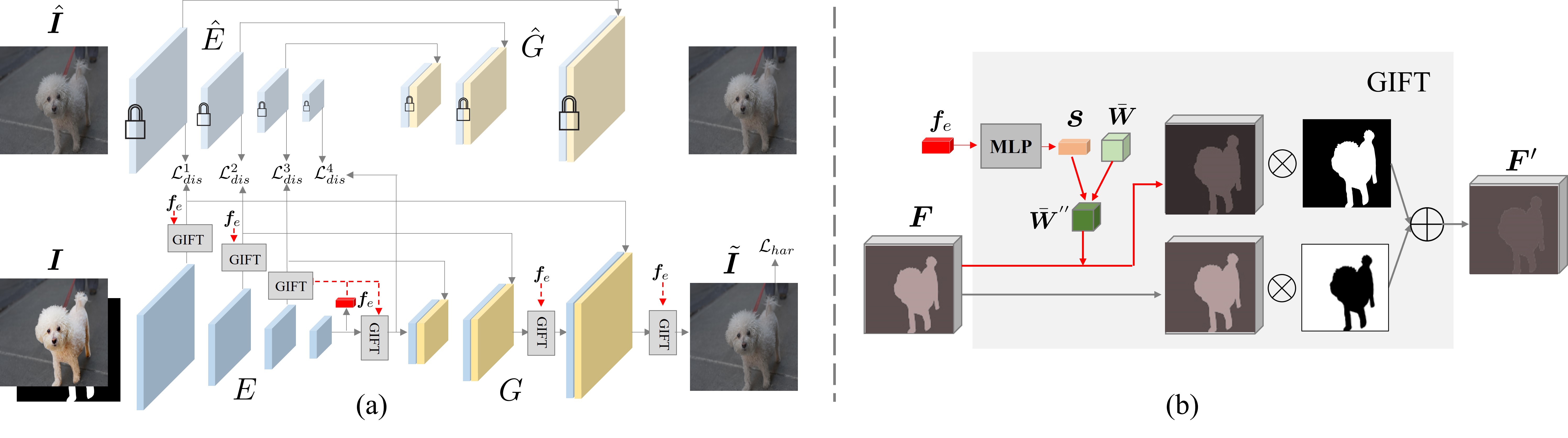
Figure 1: (a) Our network which consists of a reconstruction branch ($\hat{E},\hat{G}$) and a harmonization branch ($E,G$). The reconstruction branch is pretrained and fixed. In the harmonization branch, we use global feature $\bm{f}_{e}$ to guide feature transformation using our GIFT module. We also distill foreground-background relation from reconstruction branch to harmonization branch. (b) The detailed architecture of our GIFT module. We use global feature $\bm{f}_{e}$ to predict scale vector $\bm{s}$ and obtain the modulated convolution weights $\bar{\bm{W}}^{\prime\prime}$, which are used to adjust the foreground feature map while the background feature map remains unchanged.

We denote the composite image as $\bm{I}$, which is composed of foreground $\bm{I}^{f}$ and background $\bm{I}^{b}$. The ground-truth real image is $\hat{\bm{I}}$. The goal of image harmonization task is adjusting the composite foreground $\bm{I}^{f}$ and produce the harmonized image $\tilde{\bm{I}}$, which should be close to $\hat{\bm{I}}$. Our method is built upon the UNet-like network used in [36], which consists of an encoder $E$ with four encoder blocks, a decoder $G$ with three decoder blocks, and skip connections from the first three encoder blocks to the corresponding decoder blocks. We insert our designed globally guided feature transformation (GIFT) module into the network, which will be detailed in Section 3.1. Then, we introduce another reconstruction branch to distill the relation knowledge to the harmonization branch, which will be detailed in Section 3.2.

3.1 Globally Guided Feature Transformation

We design a globally guided feature transformation (GIFT) module, which transforms the foreground feature map using global guidance. We use $\bm{F}_{e,l}$ (resp., $\bm{F}_{d,l}$) to denote the output feature map from the $l$-th encoder (resp., decoder) block. There are four encoder blocks and thus $\bm{F}_{e,4}$ is the bottleneck feature map. We perform global average pooling over $\bm{F}_{e,4}$ and get the global feature vector $\bm{f}_{e}$, which encodes the global information beneficial for image harmonization task. We use $\bm{f}_{e}$ to guide the feature transformation for encoder/decoder feature maps. We adopt the feature transformation technique proposed in [21], which applies modulated convolution weights to the given feature map. Other feature transformation techniques are also applicable. In our task, we use global feature $\bm{f}_{e}$ to guide the modulation of convolution weights, which provides global guidance for feature transformation. Besides, we only transform the foreground feature map, since image harmonization aims to adjust the foreground to be compatible with the background.

Without loss of generality, we take one encoder/decoder feature map as an example. We have learnable base convolution weights $\bar{\bm{W}}$, in which each entry $\bar{W}(m,n,p)$ is the weight for the $m$-th input channel, $n$-th output channel, and the $p$-th spatial location. Then, we pass $\bm{f}_{e}$ through an Multi-Layer Perceptron (MLP) to predict the scale vector $\bm{s}$ corresponding to input channels. Our used MLP contains four fully-connected layers, in which the first three are shared by all feature maps and the last one is specific for each feature map. The predicted scale vector is used to modulate the base convolution weights:

$$\bar{W}^{\prime}(m,n,p)=\bar{W}(m,n,p)\cdot s(m),$$ (1)

where $s(m)$ is the $m$-th entry in $\bm{s}$ (the scale for the $m$-th input channel), and $\bar{W}^{\prime}(m,n,p)$ is the modulated weight. Next, we normalize the modulated weights following [21]:

$$\bar{W}^{\prime\prime}(m,n,p)=\frac{\bar{W}^{\prime}(m,n,p)}{\sqrt{{\sum_{m,p}\bar{W}^{\prime}(m,n,p)}^{2}+\epsilon}},$$ (2)

in which $\epsilon$ is a small constant to avoid numerical error. For more details of convolution weights modulation, please refer to [21]. Assuming that the feature map to be transformed is $\bm{F}$, which consists of the foreground feature map $\bm{F}^{f}$ and background feature map $\bm{F}^{b}$. As illustrated in Figure 1(b), we apply the modulated convolution weights $\bar{\bm{W}}^{\prime\prime}$ to the foreground feature map $\bm{F}^{f}$ and produce the transformed foreground feature map ${\bm{F}^{f}}^{\prime}$. Then, we combine ${\bm{F}^{f}}^{\prime}$ and $\bm{F}^{b}$ to obtain the transformed feature map $\bm{F}^{\prime}$.

We try applying our designed GIFT module to the output feature map from each encoder block or decoder block. We observe that the last two decoder blocks can obviously manifest the advantage of our designed GIFT, while the encoder blocks do not show clear advantage (see Section 5.3). We conjecture that the whole network is only supervised by the final ground-truth image and there is no intermediate supervision for the encoder feature maps. Lack of intermediate supervision might hinder the potential of our designed GIFT module. To provide intermediate supervision for the encoder features, we borrow the idea from knowledge distillation, which will be introduced next.

3.2 Relation Distillation

The difficulty of supervising encoder feature maps lies in the absence of ground-truth harmonized encoder feature maps. One intuitive thought is that the harmonized encoder feature maps should be close to the encoder feature maps of ground-truth real images. Therefore, besides the harmonization branch, we introduce another reconstruction branch which reconstructs the ground-truth real image $\hat{\bm{I}}$. The reconstruction branch shares similar UNet network structure (encoder $\hat{E}$ and decoder $\hat{G}$) with the harmonization branch. We denote the $l$-th encoder feature map in the reconstruction branch as $\hat{\bm{F}}_{e,l}$. Note that we perform distillation on the encoder feature maps $\bm{F}^{\prime}_{e,l}$ transformed by our GIFT module.

One naive approach is feature distillation, which enforces the encoder feature maps between two branches to be close, that is, $\hat{\bm{F}}_{e,l}$ is close to $\bm{F}^{\prime}_{e,l}$ for $l=1,\ldots,4$. However, the performance using feature distillation is unsatisfactory (see Section 5.3). One possible reason is that the encoder feature maps contain lots of redundant information and distilling the entire feature maps increases the difficulty of network training. Therefore, we turn to only distill the key information: foreground-background relation. Distilling foreground-background relation can ensure that the foreground feature map is compatible with the background feature map in $\bm{F}^{\prime}_{e,l}$, as in $\hat{\bm{F}}_{e,l}$.

There could be many possible ways to characterize foreground-background relation. To avoid the heavy computational cost of pixel-to-pixel relation, we first calculate the averaged foreground feature and then calculate the similarity between it and pixel-wise features. By taking $\bm{F}^{\prime}_{e,l}$ as an example, we calculate the averaged foreground feature $\bm{f}^{\prime}_{e,l}$ by performing average pooling within the foreground region. Then, we calculate the similarity between $\bm{f}^{\prime}_{e,l}$ and the $i$-th pixel-wise feature in $\bm{F}^{\prime}_{e,l}$ as follows,

$$R^{\prime}_{l}[i]=\frac{\exp(-\gamma\|\bm{f}^{\prime}_{e,l}-\bm{F}^{\prime}_{e,l}[i]\|^{2})}{\sum_{j}\exp(-\gamma\|\bm{f}^{\prime}_{e,l}-\bm{F}^{\prime}_{e,l}[j]\|^{2})},$$ (3)

in which $\gamma$ is a hyper-parameter. The similarities $R^{\prime}_{l}[i]$ of all pixels form a similarity map $\bm{R}^{\prime}_{l}$, in which the values in the background region represent the relation between foreground and background. The background regions with similar appearance to the foreground should have higher values. The similarity map $\hat{\bm{R}}_{l}$ for $\hat{\bm{F}}_{e,l}$ could be calculated in a similar way. Then, we distill foreground-background relation from $\hat{\bm{F}}_{e,l}$ to $\bm{F}^{\prime}_{e,l}$ using the distillation loss $\mathcal{L}^{l}_{dis}=\|\bm{R}^{\prime}_{l}-\hat{\bm{R}}_{l}\|^{2}$, which pushes the foreground-background relation in the harmonized feature map towards that in the real feature map, so that foreground is compatible with the background in the harmonized feature map.

During training, we first train and fix the reconstruction branch. Then, we train the harmonization branch. In addition to the distillation loss, we enforce the harmonized image $\tilde{\bm{I}}$ to be close to the ground-truth image $\hat{\bm{I}}$ by $\mathcal{L}_{har}=\|\tilde{\bm{I}}-\hat{\bm{I}}\|_{1}$.

After summing up the distillation losses for four encoder blocks, the total loss for the harmonization branch is

$$\mathcal{L}_{all}=\mathcal{L}_{har}+\lambda\sum_{l=1}^{4}\mathcal{L}^{l}_{dis},$$ (4)

in which $\lambda$ is a hyper-parameter.

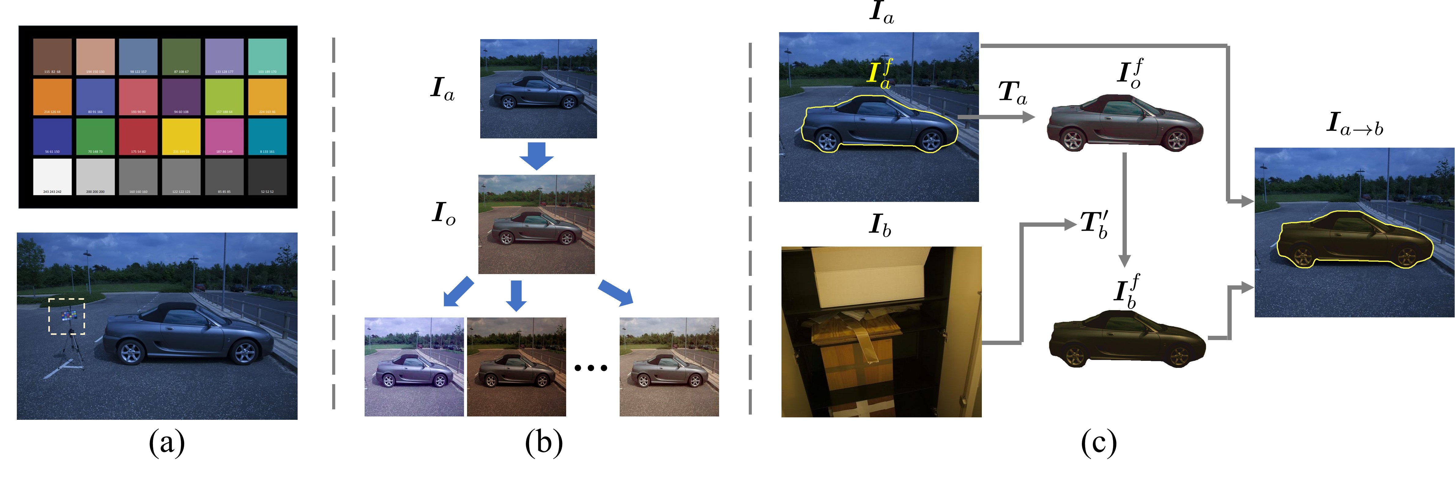
Figure 2: (a) A color checker in standard illumination condition and an image captured with color checker (see the yellow bounding box). (b) We first convert $\bm{I}_{a}$ to $\bm{I}_{o}$ in standard illumination condition, and then convert $\bm{I}_{o}$ to other illumination conditions. (c) The construction process of our dataset. Given a real image $\bm{I}_{a}$, we convert its foreground $\bm{I}_{a}^{f}$ to $\bm{I}_{o}^{f}$ in standard illumination condition using polynomial matching matrix $\bm{T}_{a}$. Then, we convert $\bm{I}_{o}^{f}$ to $\bm{I}_{b}^{f}$ in the illumination condition of reference image $\bm{I}_{b}$ using the inverse polynomial matching matrix $\bm{T}^{\prime}_{b}$. Finally, $\bm{I}_{b}^{f}$ is combined with the background of $\bm{I}_{a}$ to produce a synthetic composite image $\bm{I}_{a\rightarrow b}$.

4 Our ccHarmony Dataset

In this work, we explore a novel transitive way to construct image harmonization dataset, aiming to simulate the natural illumination variation. Specifically, based on the existing datasets with recorded illumination information, we first convert the foreground in a real image to the standard illumination condition, and then convert it to another illumination condition, which is combined with the original background to produce a synthetic composite image.

We build our dataset upon two publicly datasets with recorded illumination information: NUS dataset [7] and Gehler dataset [12], which were originally constructed for the research on color constancy. In these two datasets, each image is captured with a color checker placed in the scene that provides ground-truth reference for illumination estimation. Given a 24-patch Macbeth color checker, we have the original colors of 24 patches in standard illumination condition (see Figure 2(a)), which is referred to as standard patch color. Given an image with color checker, we can extract the colors of 24 patches, which is referred to as image patch color.

Inspired by previous works [48, 30, 1], we use polynomial matching to characterize the color transformation between standard patch colors and image patch colors. Formally, we denote the standard patch colors of 24 patches as $\mathcal{C}_{o}=\{\bm{c}^{o}_{1},\bm{c}^{o}_{2},\ldots,\bm{c}^{o}_{24}\}$ and image patch colors of 24 patches in image $\bm{I}_{a}$ as $\mathcal{C}_{a}=\{\bm{c}^{a}_{1},\bm{c}^{a}_{2},\ldots,\bm{c}^{a}_{24}\}$. We can learn a polynomial matching matrix $\bm{T}_{a}$ which converts $\mathcal{C}_{a}$ to $\mathcal{C}_{o}$. $\bm{T}_{a}$ could convert $\bm{I}_{a}$ to $\bm{I}_{o}$ in standard illumination condition. We can also learn an inverse polynomial matching matrix $\bm{T}^{\prime}_{a}$ which converts $\mathcal{C}_{o}$ to $\mathcal{C}_{a}$. Provided with inverse polynomial matching matrices from other images, we can convert $\bm{I}_{o}$ to the illumination conditions of other images. As shown in Figure 2(b), with standard illumination condition being the transitional state, we can transfer across different illumination conditions to simulate natural illumination variation.

Next, we briefly describe our way of creating synthetic composite images. As depicted in Figure 2(c), given an image $\bm{I}_{a}$ with foreground mask, we convert its foreground $\bm{I}_{a}^{f}$ to the one $\bm{I}_{o}^{f}$ in standard illumination condition using polynomial matching matrix $\bm{T}_{a}$. Next, by using the inverse polynomial matching matrix $\bm{T}^{\prime}_{b}$ of another reference image $\bm{I}_{b}$, we convert $\bm{I}_{o}^{f}$ to $\bm{I}_{b}^{f}$ in the illumination condition of $\bm{I}_{b}$. Finally, we replace the foreground $\bm{I}_{a}^{f}$ in $\bm{I}_{a}$ with its counterpart $\bm{I}_{b}^{f}$, yielding a synthetic composite image $\bm{I}_{a\rightarrow b}$. In this manner, we can acquire adequate pairs of synthetic composite images and real images like $\{\bm{I}_{a\rightarrow b},\bm{I}_{a}\}$. Because our dataset is constructed based on images with color checker (cc), we name our dataset as ccHarmony. The details of our dataset construction are left to supplementary due to space limitation.

5 Experiments

5.1 Datasets and Implementation Details

Method	All			HCOCO			HFlickr			HAdobe5k			Hday2night
	MSE	fMSE	PSNR	MSE	fMSE	PSNR	MSE	fMSE	PSNR	MSE	fMSE	PSNR	MSE	fMSE	PSNR
DoveNet [10]	52.36	549.96	34.75	36.72	554.55	35.83	133.14	832.64	30.21	52.32	383.91	34.34	54.05	1075.42	35.18
RainNet [29]	40.29	469.60	36.12	31.12	535.40	37.08	117.59	751.12	31.64	42.85	320.43	36.22	47.24	852.12	34.83
IIH [16]	38.71	400.29	35.90	24.92	416.38	37.16	105.13	716.60	31.34	43.02	284.21	35.20	55.53	797.04	35.96
IHT [15]	27.89	295.56	37.94	14.98	274.67	39.22	67.88	471.04	33.55	36.83	242.57	37.17	49.67	736.55	36.38
iSSAM [36]	24.64	262.67	37.95	16.48	266.14	39.16	69.68	443.63	33.56	22.59	166.19	37.24	40.59	591.07	37.72
CDTNet [9]	23.75	252.05	38.23	16.25	261.29	39.15	68.61	423.03	33.55	20.62	149.88	38.24	36.72	549.47	37.95
Harmonizer [22]	24.26	280.51	37.84	17.34	298.42	38.77	64.81	434.06	33.63	21.89	170.05	37.64	33.14	542.07	37.56
DCCF [44]	22.05	266.49	38.50	14.87	272.09	39.52	60.41	411.53	33.94	19.90	175.82	38.27	49.32	655.43	37.88
GiftNet	19.46	225.30	38.92	12.70	229.68	39.91	54.33	360.08	34.44	18.35	143.96	38.76	38.28	566.47	37.81

Table 1: Quantitative comparison on iHarmony4 [10] dataset. The best results are denoted in boldface.

We conduct experiments on the benchmark iHarmony4 [10] and our constructed ccHarmony dataset. iHarmony4 [10] is composed of four sub-datasets: HCOCO, HFlickr, HAdobe5K, Hday2night, which contains totally $65,742$ (resp., $7,404$) pairs of composite images and ground-truth real images in the training (resp., test) set. Following previous works [10, 36], we merge the training sets of four subdatasets as the whole training set and evaluate on each subdataset. Our constructed ccHarmony dataset has $3,080$ (resp., $1,180$) pairs of composite images and ground-truth real images in the training (resp., test) set. For the experiments on ccHarmony, we first pretrain the model on iHarmony4 [10] and then finetune the model on ccHarmony, in which the input image size is set as $256\times 256$.

For evaluation metrics, following previous works [10, 36, 16, 9], we adopt PSNR, MSE, fMSE, fSSIM, in which fMSE (resp., fSSIM) means MSE (resp., SSIM) within the foreground region. Our model is implemented using Pytorch 1.10.1 and trained using Adam optimizer with learning rate being $1e{-3}$ on ubuntu 20.04 operation system, Intel(R) Xeon(R) Silver 4116 CPU, and RTX 3090 GPUs with 24GB memory. We empirically set $\gamma$ as $0.01$ and $\lambda$ as $0.001$.

5.2 Comparison with Baselines

On iHarmony4, we compare with following image harmonization methods: DoveNet [36], RainNet [29], IIH [16], IHT [15], iSSAM [36], CDTNet [9], Harmonizer [22], DCCF [44]. In Table 1, we report the results on four sub test sets and the whole test set, which are copied from original papers or reproduced with the released models. For the overall results on the whole test set, our method outperforms the SOTA method by a large margin, e.g., 10.61% relative improvement over CDTNet on fMSE and 11.75% relative improvement over DCCF on MSE. Our method achieves the best results on HCOCO, HFlickr, HAdobe5k. Our method does not achieve satisfactory results on Hday2night, probably due to the limited training set (only $311$ images).

Method	MSE$\downarrow$	fMSE$\downarrow$	PSNR$\uparrow$	fSSIM $\uparrow$
DoveNet [10]	110.84	880.94	31.61	0.8231
RainNet [29]	58.11	519.32	34.78	0.8665
IIH [16]	83.72	636.28	33.64	0.7640
IHT [15]	55.73	514.47	35.07	0.8203
iSSAM [36]	28.83	264.84	36.05	0.9096
CDTNet [9]	27.87	264.51	36.62	0.9225
Harmonizer [22]	43.31	402.09	34.68	0.8951
DCCF [44]	29.25	259.83	36.62	0.9094
GiftNet	24.55	235.20	37.59	0.9322

Table 2: Quantitative comparison on our ccHarmony dataset. The best results are denoted in boldface.

On ccHarmony, we also report the results of our method and baselines in Table 2. Again, our method outperforms the baselines and achieves significant improvement.

For the competitive baselines [36, 9, 22, 44] and our method, we show the harmonized results on iHarmony4 in Figure 3 and the results on ccHarmony in Figure 4. Our method can usually produce visually pleasant results which are closer to the ground-truth real images. More visualization results can be found in the supplementary.

Row	GIFT		Distill		Evaluation
	Layer	Op	Layer	Op	MSE	fMSE	PSNR
1					24.64	262.67	37.95
2	$D_{3}$	*			21.39	243.23	38.71
3	$D_{2,3}$	*			20.82	238.89	38.76
4	$D_{1,2,3}$	*			20.79	237.06	38.78
5	$D_{2,3},E$	*			20.50	236.22	38.77
6	$D_{3}$	w/o g			24.33	263.22	38.18
7	$D_{3}$	$D_{3}\!\rightarrow$g			24.21	261.15	38.28
8	$D_{2,3},E$	*	$E$	*	19.46	225.30	38.92
9	$D_{2,3},E$	*	$D_{2,3},E$	*	21.31	242.58	38.73
10	$D_{2,3},E$	*	$E$	FD	21.58	240.18	38.67

Table 3: Ablation studies on iHarmony4 [10] dataset. * means the default operation. $D_{k}$ means the $k$-th decoder block. $E$ means all encoder blocks. “FD” is short for feature distillation. “w/o g” means without guidance. “$D_{3}\!\rightarrow$g” means using $D_{3}$ feature map as guidance. The best results are denoted in boldface.

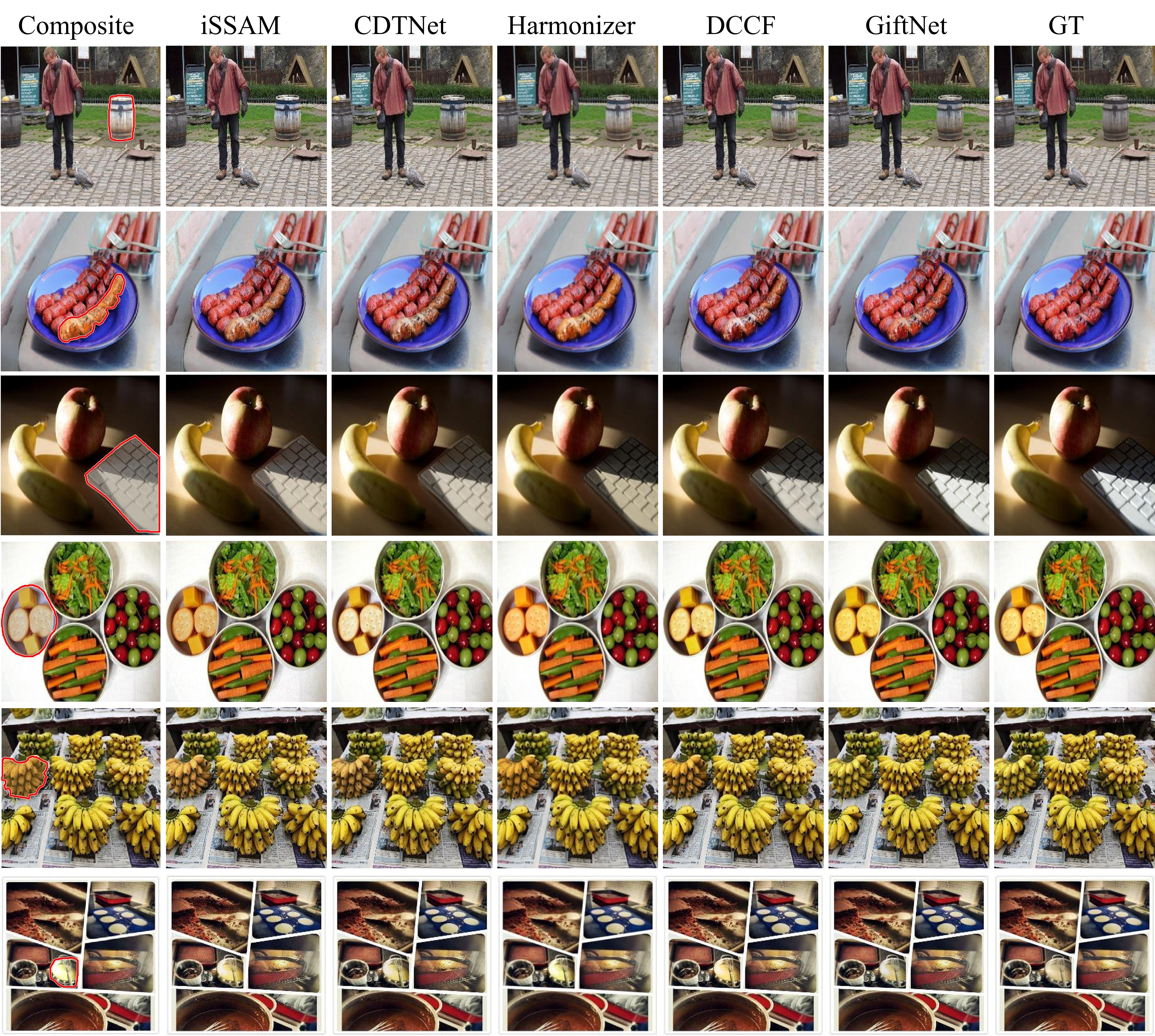
Figure 3: From left to right, we show the composite image (foreground outlined in red), the harmonized results of iSSAM [36], CDTNet [9], Harmonizer [22], DCCF [44], our GiftNet, and the ground-truth on iHarmony4 [10] dataset.

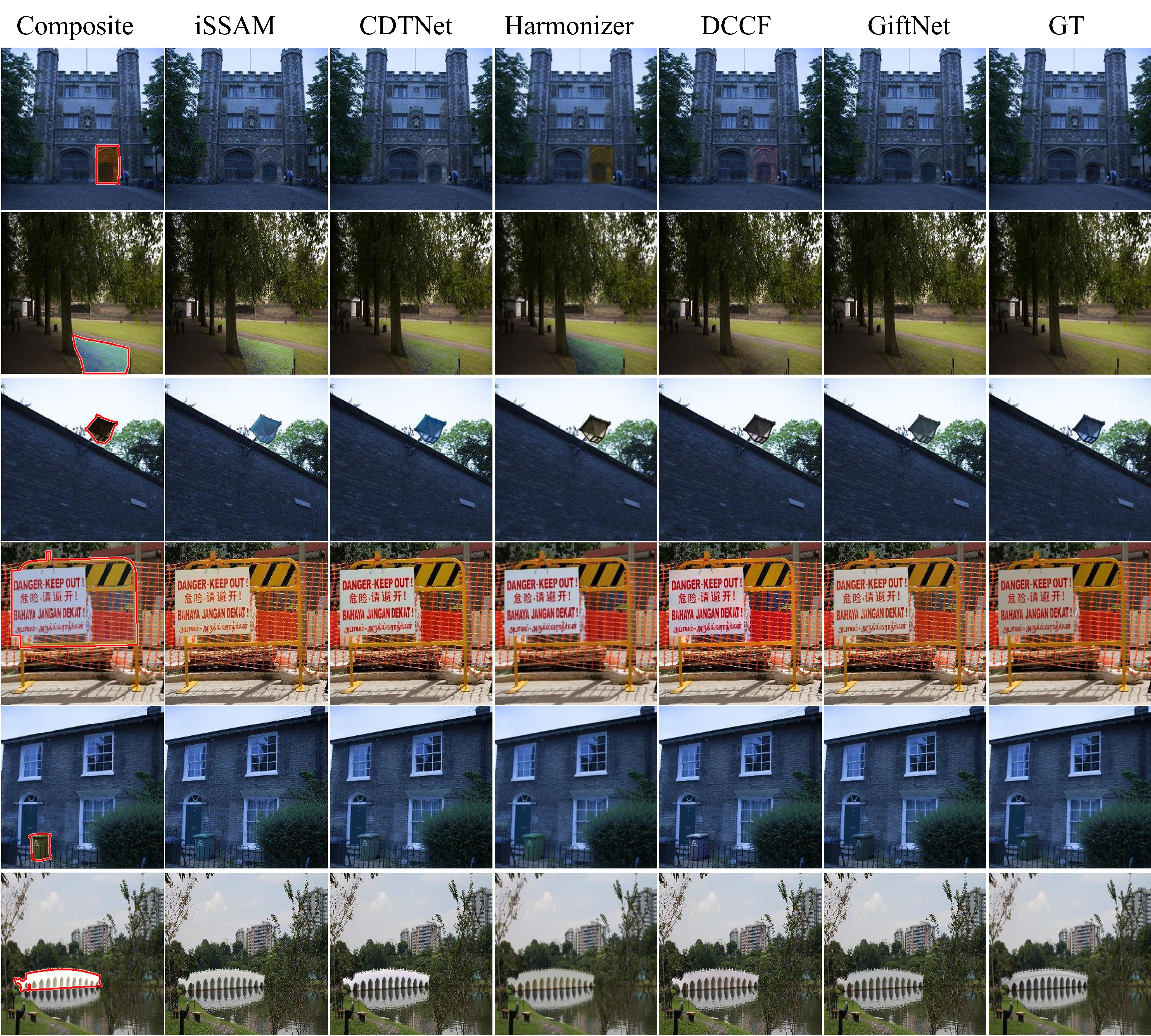
Figure 4: From left to right, we show the composite image (foreground outlined in red), the harmonized results of iSSAM [36], CDTNet [9], Harmonizer [22], DCCF [44], our GiftNet, and the ground-truth on our ccHarmony dataset.

5.3 Ablation Studies

We conduct ablation studies and report the results in Table 3. After removing GIFT module and relation distillation, our network reduces to [36], so we include the results of [36] in row 1 as the performance of basic model.

GIFT Module: We first investigate the effectiveness of our GIFT module. Recall that we have four encoder blocks and three decoder blocks. We first append GIFT module to each encoder block or decoder block. We observe that appending GIFT module to the last decoder block achieves the largest improvement. For brevity, we only report the performance of appending to the last decoder block ($D_{3}$ in row 2) in Table 3. Based on row 2, we further append GIFT module to the penultimate decoder block ($D_{2,3}$ in row 3) and the performance gain is relatively small. Then, we further append GIFT module to the first decoder block ($D_{1,2,3}$ in row 4) or the encoder blocks ($E$ in row 5), but the performance gains are very marginal.

Based on row 2, we compare with other types of guidance information for modulating convolution weights. The first type is no guidance information, that is, we use the same learnable input channel scales for all images. The performance is only comparable with row 1, which shows that simply adding more convolution layers does not work. The second type is using the feature map to be transformed to predict the input channel scales. In the case of $D_{3}$, we perform average pooling over the last decoder feature map and pass the averaged feature vector through an MLP to predict the input channel scales. Again, there is no obvious improvement over row 1, demonstrating the necessity of using global information to guide feature transformation.

Relation Distillation: Based on row 5, we add relation distillation to encoder feature maps and observe slight performance improvement (row 8 v.s. row 5). We also try adding relation distillation to decoder feature maps, but the performance becomes worse (row 9 v.s. row 8). One possible reason is that the supervision from the final ground-truth image is sufficient to learn effective decoder features, whereas the relation distillation may disturb the learning of decoder features. Therefore, we only employ relation distillation on encoder feature maps. We also compare relation distillation with feature distillation. In particular, we replace relation distillation loss with feature distillation loss. The obtained performance in row 10 is not satisfactory, which demonstrates the superiority of relation distillation. As explained in Section 1, the whole feature maps contain much redundant and noisy information, which may enlarge the training difficulty of network. In contrast, relation distillation solely distills the key information for image harmonization task.

Method	Composite	iSSAM [36]	CDTNet [9]	Harmonizer [22]	DCCF [44]	GiftNet
B-T score	-1.075	0.0755	0.212	0.117	0.235	0.436

Table 4: B-T scores of different methods on $100$ real composite images [9].

5.4 Real Composite Images

We additionally compare different methods on $100$ real composite images provided by [9]. Since there are no ground-truth for these real composite images, we conduct user study to compare with competitive baselines [36, 9, 22, 44]. Following [9], given each composite image and its $5$ harmonized results from different methods ($4$ baselines and our method), we can create image pairs by randomly choosing $2$ images from $6$ images ($5$ harmonized results and one composite image). Thus, we can construct $1500$ image pairs based on $100$ real composite images. We ask $50$ users to watch an image pair each time and choose the more harmonious image, leading to $75,000$ pairwise results. Then, we use the Bradley-Terry (B-T) model [3, 23] to calculate the global ranking of all methods, as reported in Table 4. Our method achieves the highest B-T score, which demonstrates the effectiveness of globally guided feature transformation and relation distillation. The visualization results on real composite images are left to the supplementary due to space limitation.

6 Conclusion

In this work, we have proposed globally guided feature transformation and relation distillation for image harmonization. We have also contributed a new dataset named ccHarmony, which provides a new perspective for harmonization dataset construction. Comprehensive experiments have demonstrated the superiority of our method.

References

- [1] Mahmoud Afifi, Brian Price, Scott Cohen, and Michael S Brown. When color constancy goes wrong: Correcting improperly white-balanced images. In CVPR, 2019.
- [2] Zhongyun Bao, Chengjiang Long, Gang Fu, Daquan Liu, Yuanzhen Li, Jiaming Wu, and Chunxia Xiao. Deep image-based illumination harmonization. In CVPR, 2022.
- [3] Ralph Allan Bradley and Milton E Terry. Rank analysis of incomplete block designs: I. the method of paired comparisons. Biometrika, 1952.
- [4] Junyan Cao, Wenyan Cong, Li Niu, Jianfu Zhang, and Liqing Zhang. Deep image harmonization by bridging the reality gap. BMVC, 2022.
- [5] Junyan Cao, Yan Hong, and Li Niu. Painterly image harmonization in dual domains. In AAAI, 2023.
- [6] Bor-Chun Chen and Andrew Kae. Toward realistic image compositing with adversarial learning. In CVPR, 2019.
- [7] Dongliang Cheng, Dilip K Prasad, and Michael S Brown. Illuminant estimation for color constancy: why spatial-domain methods work and the role of the color distribution. JOSA A, 31(5):1049–1058, 2014.
- [8] Wenyan Cong, Li Niu, Jianfu Zhang, Jing Liang, and Liqing Zhang. BargainNet: Background-guided domain translation for image harmonization. In ICME, 2021.
- [9] Wenyan Cong, Xinhao Tao, Li Niu, Jing Liang, Xuesong Gao, Qihao Sun, and Liqing Zhang. High-resolution image harmonization via collaborative dual transformations. CVPR, 2022.
- [10] Wenyan Cong, Jianfu Zhang, Li Niu, Liu Liu, Zhixin Ling, Weiyuan Li, and Liqing Zhang. Dovenet: Deep image harmonization via domain verification. In CVPR, 2020.
- [11] Xiaodong Cun and Chi-Man Pun. Improving the harmony of the composite image by spatial-separated attention module. IEEE Trans. Image Process., 29:4759–4771, 2020.
- [12] Peter Vincent Gehler, Carsten Rother, Andrew Blake, Tom Minka, and Toby Sharp. Bayesian color constancy revisited. In CVPR, 2008.
- [13] Jianping Gou, Baosheng Yu, Stephen J Maybank, and Dacheng Tao. Knowledge distillation: A survey. International Journal of Computer Vision, 129(6):1789–1819, 2021.
- [14] Zonghui Guo, Zhaorui Gu, Bing Zheng, Junyu Dong, and Haiyong Zheng. Transformer for image harmonization and beyond. IEEE Transactions on Pattern Analysis and Machine Intelligence, 2022.
- [15] Zonghui Guo, Dongsheng Guo, Haiyong Zheng, Zhaorui Gu, Bing Zheng, and Junyu Dong. Image harmonization with transformer. In ICCV, 2021.
- [16] Zonghui Guo, Haiyong Zheng, Yufeng Jiang, Zhaorui Gu, and Bing Zheng. Intrinsic image harmonization. In CVPR, 2021.
- [17] Yucheng Hang, Bin Xia, Wenming Yang, and Qingmin Liao. Scs-co: Self-consistent style contrastive learning for image harmonization. In CVPR, 2022.
- [18] Guoqing Hao, Satoshi Iizuka, and Kazuhiro Fukui. Image harmonization with attention-based deep feature modulation. In BMVC, 2020.
- [19] Geoffrey Hinton, Oriol Vinyals, and Jeff Dean. Distilling the knowledge in a neural network. arXiv preprint arXiv:1503.02531, 2015.
- [20] Yifan Jiang, He Zhang, Jianming Zhang, Yilin Wang, Zhe Lin, Kalyan Sunkavalli, Simon Chen, Sohrab Amirghodsi, Sarah Kong, and Zhangyang Wang. Ssh: A self-supervised framework for image harmonization. In ICCV, 2021.
- [21] Tero Karras, Samuli Laine, Miika Aittala, Janne Hellsten, Jaakko Lehtinen, and Timo Aila. Analyzing and improving the image quality of stylegan. In CVPR, 2020.
- [22] Zhanghan Ke, Chunyi Sun, Lei Zhu, Ke Xu, and Rynson WH Lau. Harmonizer: Learning to perform white-box image and video harmonization. In ECCV, 2022.
- [23] Wei-Sheng Lai, Jia-Bin Huang, Zhe Hu, Narendra Ahuja, and Ming-Hsuan Yang. A comparative study for single image blind deblurring. In CVPR, 2016.
- [24] Jean-François Lalonde and Alexei A. Efros. Using color compatibility for assessing image realism. In ICCV, 2007.
- [25] Edwin H Land. The retinex theory of color vision. Scientific american, 237(6):108–129, 1977.
- [26] Edwin H Land and John J McCann. Lightness and retinex theory. Josa, 61(1):1–11, 1971.
- [27] Quanquan Li, Shengying Jin, and Junjie Yan. Mimicking very efficient network for object detection. In CVPR, 2017.
- [28] Jingtang Liang, Xiaodong Cun, and Chi-Man Pun. Spatial-separated curve rendering network for efficient and high-resolution image harmonization. In ECCV, 2022.
- [29] Jun Ling, Han Xue, Li Song, Rong Xie, and Xiao Gu. Region-aware adaptive instance normalization for image harmonization. In CVPR, 2021.
- [30] Hang Luo and Xiaoxia Wan. Estimating polynomial coefficients to correct improperly white-balanced srgb images. IEEE Signal Processing Letters, 28:1709–1713, 2021.
- [31] Li Niu, Wenyan Cong, Liu Liu, Yan Hong, Bo Zhang, Jing Liang, and Liqing Zhang. Making images real again: A comprehensive survey on deep image composition. arXiv preprint arXiv:2106.14490, 2021.
- [32] Nikolaos Passalis, Maria Tzelepi, and Anastasios Tefas. Heterogeneous knowledge distillation using information flow modeling. In CVPR, 2020.
- [33] Jinlong Peng, Zekun Luo, Liang Liu, Boshen Zhang, Tao Wang, Yabiao Wang, Ying Tai, Chengjie Wang, and Weiyao Lin. Frih: Fine-grained region-aware image harmonization. arXiv preprint arXiv:2205.06448, 2022.
- [34] Xuqian Ren and Yifan Liu. Semantic-guided multi-mask image harmonization. In ECCV, 2022.
- [35] Adriana Romero, Nicolas Ballas, Samira Ebrahimi Kahou, Antoine Chassang, Carlo Gatta, and Yoshua Bengio. Fitnets: Hints for thin deep nets. arXiv preprint arXiv:1412.6550, 2014.
- [36] Konstantin Sofiiuk, Polina Popenova, and Anton Konushin. Foreground-aware semantic representations for image harmonization. In WACV, 2021.
- [37] Shuangbing Song, Fan Zhong, Xueying Qin, and Changhe Tu. Illumination harmonization with gray mean scale. In CGI, 2020.
- [38] Kalyan Sunkavalli, Micah K. Johnson, Wojciech Matusik, and Hanspeter Pfister. Multi-scale image harmonization. ACM Transactions on Graphics, 29(4):125:1–125:10, 2010.
- [39] Yi-Hsuan Tsai, Xiaohui Shen, Zhe Lin, Kalyan Sunkavalli, Xin Lu, and Ming-Hsuan Yang. Deep image harmonization. In CVPR, 2017.
- [40] Jeya Maria Jose Valanarasu, He Zhang, Jianming Zhang, Yilin Wang, Zhe Lin, Jose Echevarria, Yinglan Ma, Zijun Wei, Kalyan Sunkavalli, and Vishal M Patel. Interactive portrait harmonization. ICLR, 2023.
- [41] Xiaochuan Wang, Aiguo Chen, Liang Zhang, Yi Gu, Mang Xu, and Haoyuan Yan. Distilling the knowledge of multiscale densely connected deep networks in mechanical intelligent diagnosis. WCMC, 2021, 2021.
- [42] Xiaobo Wang, Tianyu Fu, Shengcai Liao, Shuo Wang, Zhen Lei, and Tao Mei. Exclusivity-consistency regularized knowledge distillation for face recognition. In ECCV, 2020.
- [43] Yazhou Xing, Yu Li, Xintao Wang, Ye Zhu, and Qifeng Chen. Composite photograph harmonization with complete background cues. In ACM MM, 2022.
- [44] Ben Xue, Shenghui Ran, Quan Chen, Rongfei Jia, Binqiang Zhao, and Xing Tang. Dccf: Deep comprehensible color filter learning framework for high-resolution image harmonization. In ECCV, 2022.
- [45] Su Xue, Aseem Agarwala, Julie Dorsey, and Holly E. Rushmeier. Understanding and improving the realism of image composites. ACM Transactions on Graphics, 31(4):84:1–84:10, 2012.
- [46] Junho Yim, Donggyu Joo, Jihoon Bae, and Junmo Kim. A gift from knowledge distillation: Fast optimization, network minimization and transfer learning. In CVPR, 2017.
- [47] Feng Zhang, Xiatian Zhu, and Mao Ye. Fast human pose estimation. In CVPR, 2019.
- [48] Yingjie Zhou, Kun Gao, Yue Guo, Zeyang Dou, Haobo Cheng, and Zhuoyi Chen. Color correction method for digital camera based on variable-exponent polynomial regression. In Communications, Signal Processing, and Systems: Proceedings of the 2018 CSPS Volume II: Signal Processing 7th, pages 111–118, 2020.
- [49] Ziyue Zhu, Zhao Zhang, Zheng Lin, Ruiqi Wu, Zhi Chai, and Chun-Le Guo. Image harmonization by matching regional references. arXiv preprint arXiv:2204.04715, 2022.