Trajectory Optimization for Cellular-Enabled UAV with Connectivity and Battery Constraints

Abstract

In this paper, we address the problem of path planning for a cellular-enabled UAV with connectivity and battery constraints. The UAV’s mission is to deliver a payload from an initial point to a final point as soon as possible, while maintaining connectivity with a BS and adhering to the battery constraint. The UAV’s battery can be replaced by a fully charged battery at a charging station, which may take some time depending on waiting time. Our key contribution lies in proposing an algorithm that efficiently computes an optimal UAV path in polynomial time. We achieve this by transforming the problem into an equivalent two-level shortest path finding problem over weighted graphs and leveraging graph theoretic approaches. In more detail, we first find an optimal path and speed to travel between each pair of charging stations without replacing the battery, and then find the optimal order of visiting charging stations. To demonstrate the effectiveness of our approach, we compare it with previously proposed algorithms and show that our algorithm outperforms those in terms of both computational complexity and performance. Furthermore, we propose another algorithm that computes the maximum payload weight that the UAV can deliver under the connectivity and battery constraints.

I Introduction

Unmanned aerial vehicles (UAVs) are widely used in various scenarios, including delivery or transportation [2], aerial surveillance and monitoring [3], flying base stations (BSs) [4], and data collection and/or power transfer for IoT devices [5, 6], due to their high mobility, free movement, and cost-effectiveness [4, 7, 8]. It has been actively studied to design the UAV trajectory according to each operational scenario. For UAV-aided communication scenarios [9, 10, 11, 6, 12, 13, 14], the UAV trajectory has been optimized taking into account various factors, e.g., minimizing energy while satisfying user-specific throughput demands [9, 10, 11, 6] or user fairness [12], and improving secrecy rate in the presence of an eavesdropper [13, 14]. For delivery or transportation scenarios, it is utmost important to swiftly and safely transport the given objects to their desired destinations. Thus, for such scenarios, the problem of designing UAV trajectory has been formulated as the minimization of the mission time with some constraints such as connectivity [15, 16, 17, 18, 19, 20, 21, 22, 23, 24, 25], restricted airspace [22, 24], collision avoidance between UAVs [24, 25], and battery constraints [26, 27, 28, 29]. In particular, it is important to track the path of UAVs, but maintaining direct communication with the control station becomes challenging when the UAV travels over long distances, due to factors such as large path loss and low line-of-sight probability [30, 31]. A promising solution to this problem is cellular-enabled UAV communication [15], wherein the UAV communicates with its control station by connecting with a close BS and the underlying cellular network [32].

In this paper, we address the problem of path planning for UAVs performing delivery or transportation missions, jointly considering connectivity with the cellular network and UAV’s limited battery capacity. In the absence of battery constraint, the problem of minimizing the mission time while maintaining the connectivity with the cellular network has been extensively studied [15, 16, 17, 18, 19, 20, 21, 22, 23, 25, 24]. In the work [15], the authors focused on optimizing the trajectory between an initial and a final location while maintaining communication with a base station (BS). They simplified the problem by assuming that the UAV can connect with a BS if the distance between them is less than a certain threshold. By doing so, they converted the problem into equivalent convex optimization and graph-theoretic path finding problems, and proposed one optimal (NP-hard) and two sub-optimal (NP-easy) algorithms. The study of characterizing an optimal path under the connectivity constraint has been extended in various directions, e.g., allow a certain duration or ratio of communication outage [16, 17], consider 3-dimensional (3D) space [18, 19], and consider the collaboration of multiple UAVs [20]. In particular, the work [17] introduced an intersection method, which effectively reduces the time complexity by converting the problem into a graph-theoretic path finding problem whose vertex set consists of the intersection points of the coverage boundaries of the BSs. Moreover, the work [19] also used a graph theoretic approach even for 3D path finding problem with a realistic communication environment considering signal blockage and reflection by buildings and interference from other BSs, by quantizing the radio map to finite grid points. On the other hand, for scenarios with limited prior knowledge about the communication environment, reinforcement learning (RL) [33] based approaches become effective, as they can approximate the communication environment empirically. The use of RL-based UAV path planning has been explored in several works [21, 22, 23, 25, 24]. However, note that the optimal path may not always be derived using the RL-based approach, and the training phase of RL can be time-consuming and resource-intensive.

In practice, it is important to consider the limited battery capacity of the UAV. There have been a few works on designing UAV trajectory performing delivery or transportation missions taking into account the limited battery capacity [26, 27, 28, 29]. The work [26] considered a variant of the travelling salesman problem (TSP) that aims to derive a shortest route visiting each target node once, while considering the limited battery capacity of the UAV and charging stations to replenish its energy. Such a UAV route optimization problem with TSP formulation taking into account the battery constraint has been extended by considering multiple UAVs [27, 28] and grouping target nodes into clusters [29]. However, the problem of designing an optimal UAV path under both the connectivity and the battery constraints has not been well studied.

Our key contribution lies in proposing an algorithm that efficiently computes an optimal UAV path in polynomial time (NP-easy) to deliver a payload from an initial point to a final point as soon as possible, while maintaining connectivity with a BS and adhering to the battery constraint. We assume that the UAV can connect with a BS if they are closer than a certain threshold similarly as in [15], but we allow that the threshold can be different for each BS due to interference from other BSs. The UAV’s battery can be replaced by a fully charged battery at a charging station, which may take some time depending on waiting time [34]. The contributions of this paper are summarized as follows:

• The primary challenge in this path planning problem is optimizing the route and the speed (since the energy consumption is affected by the speed) with the decisions about when and which charging station to visit. We solve this problem by transforming the problem into an equivalent two-level shortest path finding problem over weighted graphs and leveraging graph theoretic approaches to solve it. More specifically, we first find an optimal path and speed to travel between each pair of charging stations without replacing the battery. Then, we find the optimal order of visiting charging stations to replace the battery. To demonstrate the effectiveness of our approach, we analytically compare it with previously proposed algorithms in [15, 17] that are slightly modified to meet the battery constraint. The results show that our algorithm outperforms these existing approaches in terms of both performance (mission time) and computational complexity.

• Characterizing the maximum payload weight that the UAV can deliver under the connectivity and battery constraints is another interesting problem of practical importance in delivery missions. We propose a graph theory-based algorithm that yields an optimal solution to this problem NP-easily. It first transforms the delivery environment into a weighted graph and finds the longest connectivity-critical edge between the initial and the final points in the graph. Then, it derives the largest payload weight which can be delivered over the edge without replacing the battery.

• Various numerical results are provided to show the optimal path and the corresponding delivery time according to environmental parameters and compare with the previously proposed algorithms [15, 17].

The remaining of this paper is organized as follows. In Section II, we present the system model and formulate the optimization problem of finding the fastest UAV route under the connectivity and the battery constraints. Our propose algorithms that output optimal UAV trajectories without and with the battery constraint is presented in Sections III and IV, respectively. In Section V, the problem of characterizing the maximum deliverable payload weight is formulated and an optimal algorithm for this problem is presented. We provide various numerical results in Section VI. Finally, the paper is concluded in Section VII.

II Problem Statement

We consider a cellular network with $M$ base stations (BSs) and $N\leq M$ charging stations (CSs). In this network, a UAV delivers a payload from an initial point $\mathbf{U}_{0}$ to a final point $\mathbf{U}_{F}$ under limited battery capacity. The detailed description of the UAV model is in Section II-A. The UAV should maintain the connectivity with one of the BSs while delivering the payload. The BS model and the BS-UAV connectivity is described in Section II-B. The UAV can replace its battery at a CS if needed, as explained in Section II-C. The goal of this paper is to characterize the minimum delivery time from $\mathbf{U}_{0}$ to $\mathbf{U}_{F}$, including the flight time in the air and the battery swapping time at CSs. This optimization problem is formally presented in Section II-D. The overall model is illustrated in Fig. 1.

Figure 1: An example of delivery and communication scenario of a UAV with three BSs and one CS. The UAV delivers a payload from $\mathbf{U}_{0}$ to $\mathbf{U}_{F}$ under limited battery capacity while communicating with a BS. In the CS, the UAV can replace its battery.

II-A UAV Model

In the cellular network, a rotary-wing UAV has a mission of delivering a payload from an initial point $\mathbf{U}_{0}$ to a final point $\mathbf{U}_{F}$. We assume that the UAV flies with a fixed altitude $H\in[H_{\mathrm{min}},H_{\mathrm{max}}]$, where $H_{\mathrm{min}}$ is determined by the heights of obstacles in the network and $H_{\mathrm{max}}$ corresponds to the maximum allowable altitude according to government regulations. Let us denote the 3D coordinates of $\mathbf{U}_{0}$, $\mathbf{U}_{F}$, and the UAV location at time $t$ by $(x_{0},y_{0},H)$, $(x_{F},y_{F},H)$, and $(x(t),y(t),H)$, respectively. We also denote $\mathbf{u}_{0}=(x_{0},y_{0})$, $\mathbf{u}_{F}=(x_{F},y_{F})$, and $\mathbf{u}(t)=(x(t),y(t))$ as the horizontally projected locations of the 3D coordinates. The UAV flies with time-varying speed of $v(t)\triangleq\|\nabla_{t}\mathbf{u}(t)\|$ at time $t$, where the speed is selected from the finite set $\mathcal{V}=\{0,v_{1},...,v_{q}\}$ with $0<v_{1}<...<v_{q}$.

For energy consumption, we only consider the propulsion energy consumption by the UAV, since the communication energy consumption is relatively negligible [4]. Let the total weight of UAV and its payload be given as $w=w_{1}+w_{2}+w_{3}$, where $w_{1},w_{2}$, and $w_{3}$ denote the weights of the UAV body, its battery, and the payload, respectively. The propulsion power consumption (in Watts) when flying with speed $v$ is given as

$$\begin{split}&P_{\mathrm{UAV}}(v)=P_{1}\left(1+{{3v^{2}}/{v_{\mathrm{tip}}^{2}}}\right)+P_{2}(w)\\ &\ \cdot\big{(}\sqrt{1+{{v^{4}}/{4v_{0}(w)^{4}}}}-{{v^{2}}/{2v_{0}(w)^{2}}}\big{)}^{0.5}\!\!\!+0.5{\rho}S_{\mathrm{FP}}v^{3},\end{split}$$ (1)

where $P_{1}$, $P_{2}(w)$, $v_{\mathrm{tip}}$, $v_{0}(w)$, $\rho$, and $S_{\mathrm{FP}}$ are the parameters determined by the environment of the network and the physical structure of the UAV [10]. We note that only the parameters $P_{2}(w)$ and $v_{0}(w)$ depend on the total weight $w$. The power consumption model (LABEL:eq:1) and its parameters will be revisited with details in Section VI.

The UAV consumes the energy in its battery. The battery capacity (in Joules) is expressed as follows [2]:

$$C_{\mathrm{batt}}=\epsilon_{\mathrm{batt}}w_{2},$$ (2)

where $\epsilon_{\mathrm{batt}}$ is the maximum energy of the battery per unit weight. Note that the battery capacity is directly proportional to the battery weight. As proved in [2], when the UAV flies at the same speed $v$ without replacing its battery, then the maximum distance (in meters) that it can travel is given as

$$d_{\mathrm{fly}}(v)=v\cdot{{\gamma\eta C_{\mathrm{batt}}}\over{r_{\mathrm{safe}}P_{\mathrm{UAV}}(v)}},$$ (3)

where $0<\gamma<1$ is the maximum depth of discharge of the battery, $0<\eta<1$ is the power transfer efficiency from the battery to the UAV body, and $r_{\mathrm{safe}}>1$ is the safety factor to reserve energy in the battery for unexpected situations. We note that the maximum distance in (3) is because the maximum usable energy from the fully charged battery is ${\gamma C_{\mathrm{batt}}}\over r_{\mathrm{safe}}$ (in Joules) and the UAV consumes the energy in the battery at a rate of ${P_{\mathrm{UAV}}(v)}\over{\eta}$ (in Watts).

II-B BS-UAV Connectivity

There are $M$ BSs in the cellular network. The $m$th BS where $m\in\mathcal{M}\triangleq[1:M]$, $\mathrm{BS}_{m}$ is located at $(a_{m1},a_{m2},H_{\mathrm{BS}})$, where all BSs are assumed to be located at the same altitude $H_{\mathrm{BS}}<H$. We further denote $\mathbf{a}_{m}=(a_{m1},a_{m2})$ as the horizontally projected location of $\mathrm{BS}_{m}$. Each BS has a single omni-directional antenna and the same transmission power $P_{\mathrm{tx}}$. All the BSs are connected to a control station through a backhaul network to successfully hand over from a BS to another BS and control the UAV trajectory.

We assume that the channel between the UAV and a BS is determined by the line-of-sight (LoS) probabilistic model, where the LoS probability increases as the elevation angle between the UAV and the BS increases [30]. The expected path loss between the UAV and $\mathrm{BS}_{m}$ at time $t$, $\Lambda_{m}(t)$ (in $\mathrm{dB}$) is given as $\Lambda_{m}(t)=\mathrm{FSPL}_{m}(t)+p_{m}(t)\cdot\zeta_{1}+(1-p_{m}(t))\cdot\zeta_{2}$, where $\mathrm{FSPL}_{m}(t)$ and $p_{m}(t)\in[0,1]$ are the free space path loss and the LoS probability between the UAV and $\mathrm{BS}_{m}$ at time $t$, respectively, which only depend on the distance between the UAV and $\mathrm{BS}_{m}$, and $\zeta_{1}>0$ and $\zeta_{2}>\zeta_{1}$ refer to the excessive path losses for LoS and non-LoS (NLoS) links, respectively [31]. The received signal to interference plus noise ratio (SINR) from $\mathrm{BS}_{m}$ to the UAV at time $t$ is $\mathrm{SINR}_{m}(t)={{P_{\mathrm{tx}}\cdot 10^{\Lambda_{m}(t)/10}}\over{\sum_{m^{\prime}\in\mathcal{M}\setminus m}I_{m^{\prime}m}(t)+N_{0}}}$, where $I_{m^{\prime}m}(t)$ is the interference power by $\mathrm{BS}_{m^{\prime}}$ at time $t$ when the UAV is communicating with $\mathrm{BS}_{m}$ and $N_{0}$ is the additive noise power. Note that $I_{m^{\prime}m}$ would be equal to zero if $\mathrm{BS}_{m^{\prime}}$ uses a different frequency band from $\mathrm{BS}_{m}$, and even if the two BSs use the same frequency band, it will become negligible if $\mathrm{BS}_{m^{\prime}}$ is far away from the UAV.

To maintain the control of the UAV, the communication rate from a BS to the UAV should not be less than the minimum required data rate, i.e., the maximally achievable SINR of the UAV should satisfy

$$\max_{m\in\mathcal{M}}\mathrm{SINR}_{m}(t)\geq\mathrm{SINR}_{\mathrm{th}}$$ (4)

for any time $t$ where $\mathrm{SINR}_{\mathrm{th}}$ is the hard SINR threshold to achieve the minimum required data rate. In weak interference regime, i.e., the frequency reuse factor is sufficiently low, it can be easily checked that the condition (4) can be equivalently written as $\min_{m\in\mathcal{M}}\|\mathbf{u}(t)-\mathbf{a}_{m}\|\leq d_{0}$ for some $d_{0}$, where we call $d_{0}$ the base coverage radius of each BS. For other cases, however, it is in general hard to represent the exact coverage region satisfying (4) in a simple form. For tractable analysis, we introduce the coverage offset $\lambda_{m}\in[0,d_{0}]$ for $\mathrm{BS}_{m}$ and assume that the UAV can connect with $\mathrm{BS}_{m}$ with high probability if the UAV is in the effective coverage region of $\mathrm{BS}_{m}$ given as $\|\mathbf{u}(t)-\mathbf{a}_{m}\|\leq d_{0}-\lambda_{m}$. In other words, by introducing offsets $\lambda_{m}$ taking into account the effect of interference, we assume that (4) holds with high probability if the following equation holds:

$$\min_{m\in\mathcal{M}}\|\mathbf{u}(t)-\mathbf{a}_{m}\|+\lambda_{m}\leq d_{0}.$$ (5)

II-C Charging Station Model

To deliver the payload over a long distance with limited battery capacity, the UAV may replace its battery by visiting one of $N\leq M$ CSs. The $n$th charging station $C_{n}$ where $n\in\mathcal{N}\triangleq[1:N]$ is assumed to be located at $(c_{n1},c_{n2},H_{\mathrm{CS}})$, where all CSs are assumed to be located at the same altitude $H_{\mathrm{CS}}\leq H$. We further denote $\mathbf{c}_{n}=(c_{n1},c_{n2})$ as the horizontally projected location of $C_{n}$. To reduce the delay to replace the battery, each CS uses an autonomous battery swapping system [34]. The overall delay to replace the battery at charging station $C_{n}$, $\tau_{C_{n}}\in[0,\tau_{\mathrm{max}}]$ consists of the waiting time and the battery swapping time, where $\tau_{\mathrm{max}}$ is the upper bound on the delay. We note that the waiting time at charging station $C_{n}$ varies depending on the congestion of the CS and hence $\tau_{C_{n}}$ depends on $n$.

II-D Goal

The goal of this paper is to characterize the minimum delivery time $T$ from $\mathbf{U}_{0}$ to $\mathbf{U}_{F}$ of the UAV, including the flight time in the air and the overall delay to replace its battery at CSs. The optimization problem is formulated as

Problem 1 (6)

$$\mbox{Objective:~{}}~{}~{}~{}~{}\min_{T\geq 0,\{\mathbf{u}(t),\ \psi(t),\ t\in[0,T]\}}T$$ (7)

Constraints: (8)

$$\mathbf{u}(0)=\mathbf{u}_{0},\ \mathbf{u}(T)=\mathbf{u}_{F},\ E_{\mathrm{batt}}(0)=C_{\mathrm{batt}}$$ (9)

$$\mathbf{u}(t)\in\mathbb{R}^{2},\ \psi(t)\in[0:N]$$ (10)

$$v(t)\triangleq\|\nabla_{t}\mathbf{u}(t)\|\in\mathcal{V},\ t\in[0,T]$$ (11)

$$\min_{m\in\mathcal{M}}\|\mathbf{u}(t)-\mathbf{a}_{m}\|+\lambda_{m}\leq d_{0},\ t\in[0,T]$$ (12)

$$\psi(t)=0\ \mathrm{if~{}}\mathbf{u}(t)\not\in\{\mathbf{c}_{n}|n\in\mathcal{N}\},\ t\in[0,T]$$ (13)

$$\psi(t)\in\{0,n\}\ \mathrm{if~{}}\mathbf{u}(t)\in\{\mathbf{c}_{n}|n\in\mathcal{N}\},\ t\in[0,T]$$ (14)

$$E_{\mathrm{batt}}(t)\geq(1-(\gamma/r_{\mathrm{safe}}))C_{\mathrm{batt}},\ t\in[0,T]$$ (15)

$$\nabla_{t}E_{\mathrm{batt}}(t)=\!-P_{\mathrm{UAV}}(v(t))/\eta,\ \psi(t)=0,\ t\in[0,T]$$ (16)

$$\nabla_{t}E_{\mathrm{batt}}(t)=0\ \mathrm{if~{}}\psi(t)\in\mathcal{N},\ t\in[0,T]$$ (17)

$$E_{\mathrm{batt}}(t)=C_{\mathrm{batt}}\ \mathrm{if~{}}\psi(t)\in\mathcal{N}\text{ and }$$ (18)

$$~{}~{}t-\max_{t^{\prime}}\{t^{\prime}|\psi(t^{\prime})=0,t^{\prime}\in[0,t]\}=\tau_{C_{\psi(t)}},\ t\in[0,T]$$ (19)

where $\psi(t)\in[0:N]$ is an auxiliary variable indicating whether the UAV is in charging station $C_{n}$ $(\psi(t)=n)$ or in the air $(\psi(t)=0)$ at time $t$ and $E_{\mathrm{batt}}(t)\geq 0$ is the residual energy in the battery at time $t$. Here, (9) means that the UAV departs from $\mathbf{u}_{0}$ with fully charged battery and arrives at $\mathbf{u}_{F}$ at time $T$, (10) corresponds to the range of optimizing variables, (11) denotes that the UAV can fly with a speed in the set $\mathcal{V}$, (12) is the connectivity constraint in (5), and (13)-(14) determines whether the UAV is in a CS or in the air. Next, (15) is the constraint for the maximum depth of discharge of the battery, (16) and (17) represent the power consumption when flying in the air and staying at a CS, respectively, and (19) means that the battery has the maximum energy when the battery swapping process just finished.

Note that Problem 1 is not a convex optimization problem since the variable $\psi(t)$ is selected from a discrete set and constraint (12) is not convex. Moreover, $\mathbf{u}(t)$ should be optimized in continuous $t\in[0:T]$. Such difficulties make Problem 1 non-trivial. To solve this problem, in Sections III and IV, we first reformulate Problem 1 in a framework of weighted graph and then show that the problem can be solved NP-easily by graph theory-based algorithms.

III Optimal Trajectory with the Connectivity Constraint

In this section, we provide an optimal solution for Problem 1 without the battery constraint, i.e., the battery capacity is assumed to be unlimited. We note that the UAV flies with the maximum speed $v_{q}$ from $\mathbf{U}_{0}$ to $\mathbf{U}_{F}$ since traveling with the maximum speed minimizes the mission time without the battery constraint. Such an optimization problem can be reformulated as follows:

Problem 1-1 (20)

$$\mbox{Objective: }~{}~{}\min_{T\geq 0,\{\mathbf{u}(t),\ t\in[0,T]\}}T$$ (21)

Constraints: (22)

$$\mathbf{u}(0)=\mathbf{u}_{0},\ \mathbf{u}(T)=\mathbf{u}_{F},\ \mathbf{u}(t)\in\mathbb{R}^{2}$$ (23)

$$\|\nabla_{t}\mathbf{u}(t)\|=v_{q},\ t\in[0,T]$$ (24)

$$\min_{m\in\mathcal{M}}\|\mathbf{u}(t)-\mathbf{a}_{m}\|+\lambda_{m}\leq d_{0},\ t\in[0,T]$$ (25)

Note that the optimization is still not trivial since it is non-convex and has an infinite number of variables.

To attack Problem 1-1, we propose a generalized intersection method that finds a trajectory of UAV satisfying the connectivity constraint by converting Problem 1-1 as an equivalent problem of finding the shortest path in an undirected weighted graph, and show that this generalized intersection method yields an optimal UAV path NP-easily. The pseudo code of the generalized intersection method is described in Algorithm 1.

Algorithm 1 Generalized Intersection Method

Input: $v_{q}$, $\mathbf{u}_{0}$, $\mathbf{u}_{F}$, $\mathbf{a}_{m}$, $d_{0}$, $\lambda_{m}$ for $m\in\mathcal{M}$

1:Def: Function ChkFea($\mathbf{u}_{0},\mathbf{u}_{F},\mathbf{a}_{m},d_{0},\lambda_{m}$ for $m\in\mathcal{M}$) outputs whether Problem 1-1 is feasible $(h_{\mathrm{fea}}=1)$ or not $(h_{\mathrm{fea}}=0)$, where $\mathbf{u}_{0}$ is the initial point, $\mathbf{u}_{F}$ is the final point, and $d_{0}$ and $\lambda_{m}$ for $m\in\mathcal{M}$ are the parameters about the communication environment.

2:Def: Function Dijkstra$(\mathbf{x}_{1},\mathbf{x}_{2},G)$ for graph $G=(V,E)$ outputs $(T,\mathbf{S}_{V})$, where $T$ is the minimum total weight from $\mathbf{x}_{1}\in V$ to $\mathbf{x}_{2}\in V$ over the graph $G$ and $\mathbf{S}_{V}$ is the corresponding optimal sequence of visiting nodes in $V$.

3:$V_{0}\leftarrow\{\mathbf{u}_{0},\mathbf{u}_{F}\}$, $E_{0}\leftarrow\emptyset$

4:$h_{\mathrm{fea}}\leftarrow$ ChkFea$(\mathbf{u}_{0},\mathbf{u}_{F},\mathbf{a}_{m},d_{0},\lambda_{m}$ for $m\in\mathcal{M})$

5:if $h_{\mathrm{fea}}=1$ then $\triangleright$ Problem 1-1 is feasible

6:$\triangleright$ Step 1. Vertex construction: Construct a vertex set $V_{0}$ consisting of the initial, the final, and the intersection points.

7:     for $m,m^{\prime}\in\mathcal{M}$, $m<m^{\prime}$ do

8:         if $\|\mathbf{a}_{m}-\mathbf{a}_{m^{\prime}}\|\leq 2d_{0}-\lambda_{m}-\lambda_{m^{\prime}}$ then

9:              $V_{0}\leftarrow V_{0}\cup\{\mathbf{x}\in\mathbb{R}^{2}|\ \|\mathbf{x}-\mathbf{a}_{m}\|=d_{0}-\lambda_{m},$

10:     $\|\mathbf{x}-\mathbf{a}_{m^{\prime}}\|=d_{0}-\lambda_{m^{\prime}}\}$

11:         end if

12:     end for

13:$\triangleright$ Step 2. Edge construction: Construct an edge set $E_{0}$ consisting of the line segments lying inside the set of coverage regions.

14:     for $\mathbf{x}_{1},\mathbf{x}_{2}\in V_{0}$, $\mathbf{x}_{1}\neq\mathbf{x}_{2}$ do

15:         $h_{\mathrm{out}}\leftarrow$ ChkOut$(\mathbf{x}_{1},\mathbf{x}_{2},\mathbf{a}_{m},d_{0},\lambda_{m}$ for $m\in\mathcal{M})$

16:         if $h_{\mathrm{out}}=0$ then

17:              $E_{0}\leftarrow E_{0}\cup(\mathbf{x}_{1},\mathbf{x}_{2},\|\mathbf{x}_{1}-\mathbf{x}_{2}\|/v_{q})$

18:         end if

19:     end for

20:$\triangleright$ Step 3. Path search: Find an optimal path from the initial point to the final point over the graph.

21:     $G_{0}\leftarrow(V_{0},E_{0})$ $\triangleright$ Construct graph $G_{0}$

22:     $(T,\mathbf{S}_{V_{0}})\leftarrow$ Dijkstra$(\mathbf{u}_{0},\mathbf{u}_{F},G_{0})$

23:     $\mathbf{u}(t)\text{ for }t\in[0,T]\leftarrow$ FindPath$(\mathbf{S}_{V_{0}},v_{q})$

24:else$\triangleright$ Problem 1-1 is not feasible

25:     $T\leftarrow\infty$, $\mathbf{u}(t)\leftarrow\mathrm{Null}$ for $t\in[0,T]$

26:end if

Output: ($h_{\mathrm{fea}}$, $T$, $\mathbf{u}(t)$ for $t\in[0,T]$)

This algorithm first checks (in line 3) whether the problem is feasible or not via the checking feasibility function ChkFea, which outputs whether the problem 1-1 is feasible $(h_{\mathrm{fea}}=1)$ or not $(h_{\mathrm{fea}}=0)$ according to the initial point $\mathbf{u}_{0}$, the final point $\mathbf{u}_{F}$, and the location and the effective coverage region of each BS. This function can be constructed by applying [15, Proposition 1] in the case that the BSs have the different coverage radii and its pseudo code is omitted. If the problem is feasible, an undirected weighted graph $G_{0}=(V_{0},E_{0})$ is constructed based on the intersection points of the coverage boundaries (in lines $6$-$17$). Specifically, the vertex set $V_{0}$ consists of the initial point $\mathbf{u}_{0}$, the final point $\mathbf{u}_{F}$, and the intersection points of the coverage boundaries (in lines $6$-$10$). The edge set $E_{0}$ is constructed (in lines $11$-$16$) by including a line segment $\overline{\mathbf{x}_{1}\mathbf{x}_{2}}$ between two different vertices $\mathbf{x}_{1},\mathbf{x}_{2}\in V_{0}$ if the line segment lies inside the set of coverage regions, which is checked through the function ChkOut whose pseudo code is provided in Algorithm 2 and is explained later. Such an edge is denoted by a tuple $(\mathbf{x}_{1},\mathbf{x}_{2},\|\mathbf{x}_{1}-\mathbf{x}_{2}\|/{v_{q}})$, where the weight of the edge $\|\mathbf{x}_{1}-\mathbf{x}_{2}\|/{v_{q}}$ is given by the minimum travel time between $\mathbf{x}_{1}$ and $\mathbf{x}_{2}$. After constructing a weighted undirected graph, an optimal path from $\mathbf{u}_{0}$ to $\mathbf{u}_{F}$ over the graph is derived (in lines $18$-$19$). We first find an optimal sequence $\mathbf{S}_{V_{0}}$ of visiting nodes over the graph and the corresponding weight (equal to the mission time $T$) via the Dijkstra algorithm [35] that finds the minimum weight path between two nodes over a weighted graph with low complexity. Then, the corresponding UAV trajectory can be derived through the function FindPath, which outputs the UAV trajectory according to the sequence $\mathbf{S}_{V_{0}}$ of visiting points and the speed $v_{q}$. This function can be constructed similarly as in [15, $(25)$-$(27)$] and its pseudo code is omitted. An example of the graph $G_{0}$ and the corresponding optimal trajectory by Algorithm 1 is illustrated in Fig. 2.

Figure 2: An example of graph $G_{0}$ for $M=3$. The graph has vertex set $V_{0}$ including $\mathbf{u}_{0}$, $\mathbf{u}_{F}$, and all intersection points and edge set $E_{0}$ including the (solid) line segments between two vertices which lie inside the set of coverage regions.

Algorithm 2 describes the function ChkOut which tests whether a line segment $\overline{\mathbf{x}_{1}\mathbf{x}_{2}}$ between two different vertices $\mathbf{x}_{1},\mathbf{x}_{2}\in V_{0}$ lies in the set of coverage regions. We say that the line segment experiences an outage if there exists $\xi\in[0,1]$ that satisfies the following condition:

$$\min_{m\in\mathcal{M}}\|\boldsymbol{\alpha}(\xi)-\mathbf{a}_{m}\|+\lambda_{m}>d_{0},$$ (26)

where $\boldsymbol{\alpha}(\xi)\triangleq\mathbf{x}_{1}+\xi(\mathbf{x}_{2}-\mathbf{x}_{1})$ for $\xi\in[0,1]$ represents a point in the line segment $\overline{\mathbf{x}_{1}\mathbf{x}_{2}}$. Here, (26) means that the UAV experiences an outage at point $\boldsymbol{\alpha}(\xi)$, i.g., the UAV cannot be connected with every BS at point $\boldsymbol{\alpha}(\xi)$. To check whether the line segment experiences an outage, the function ChkOut verifies whether there exists $\xi\in[0,1]$ that satisfies (26). Let us define the safe interval $\mathcal{T}_{\mathrm{safe}}\triangleq[0,\xi^{\prime}]$ for some $\xi^{\prime}\in[0,1]$ as the line segment such that every $\boldsymbol{\alpha}(\xi)$ for $\xi\in\mathcal{T}_{\mathrm{safe}}$ has been checked to be inside the coverage regions, i.e., there exists $m\in\mathcal{M}$ such that $\|\boldsymbol{\alpha}(\xi)-\mathbf{a}_{m}\|+\lambda_{m}\leq d_{0}$. The function ChkOut first checks whether $\xi=0$ is included in the coverage regions and then repeatedly updates the safe interval or declares an outage in the following way. Let the current safe interval be given as $[0,\xi^{\prime}]\subseteq[0,1]$. If the point $\boldsymbol{\alpha}(\xi^{\prime}+\epsilon)$ is checked to be connected with $\mathrm{BS}_{m}$ for sufficiently small constant $\epsilon>0$, then the safe interval is extended by including the range of $\xi$ where $\mathbf{\alpha}(\xi)$ is connected with $\mathrm{BS}_{m}$, i.e., $\|\boldsymbol{\alpha}(\xi)-\mathbf{a}_{m}\|\leq d_{0}-\lambda_{m}$. This algorithm ends if $\boldsymbol{\alpha}(\xi^{\prime}+\epsilon)$ cannot be connected with every BS $(h_{\mathrm{out}}=1)$ or the safe interval reaches $[0,1]$ $(h_{\mathrm{out}}=0)$, where $h_{\mathrm{out}}$ is the indicator whether the line segment experiences an outage $(h_{\mathrm{out}}=1)$ or not $(h_{\mathrm{out}}=0)$. An example of updating the safe interval is shown in Fig. 3.

Algorithm 2 Function ChkOut

Input: $\mathbf{x}_{1},\mathbf{x}_{2}\in V_{0},\mathbf{a}_{m},d_{0},\lambda_{m}\text{ for }m\in\mathcal{M}$

1:Def: $\boldsymbol{\alpha}(\xi)\triangleq\mathbf{x}_{1}+\xi(\mathbf{x}_{2}-\mathbf{x}_{1})$ for $\xi\in[0,1]$

2:$h_{\mathrm{out}}\leftarrow 0$, $\xi^{\prime}\leftarrow 0$, $\xi^{\prime\prime}\leftarrow 0$

3:$\epsilon\leftarrow 10^{-10}$ $\triangleright$ Sufficiently small positive constant

4:while $\xi^{\prime}<1$ do

5:$\triangleright$ Update safe interval $\mathcal{T}_{\mathrm{safe}}$ from $[0,\xi^{\prime}]$ to $[0,\xi^{\prime\prime}]$ if $\boldsymbol{\alpha}(\xi^{\prime}+\epsilon)$ is included in the set of coverage regions.

6:     for $m\in\mathcal{M}$ do $\triangleright$ Find BS which covers $\boldsymbol{\alpha}(\xi^{\prime}+\epsilon)$.

7:         if $\|\boldsymbol{\alpha}(\xi^{\prime}+\epsilon)-\mathbf{a}_{m}\|\leq d_{0}-\lambda_{m}$ then

8:              $\xi^{\prime\prime}\!\leftarrow\!\max\{\xi\in[0,1]|\ \|\boldsymbol{\alpha}(\xi)-\mathbf{a}_{m}\|\leq d_{0}-\lambda_{m}\}$

9:              break

10:         end if

11:     end for

12:     if $\xi^{\prime\prime}=\xi^{\prime}$ then $\triangleright$ $\boldsymbol{\alpha}(\xi^{\prime}+\epsilon)$ experiences an outage.

13:         $h_{\mathrm{out}}\leftarrow 1$

14:         break

15:     end if

16:     $\xi^{\prime}\leftarrow\xi^{\prime\prime}$

17:end while$\triangleright$ $\xi^{\prime}=1$ means that $\mathcal{T}_{\mathrm{safe}}=[0,1]$.

Output: $h_{\mathrm{out}}$

Figure 3: An example of updating the safe interval $\mathcal{T}_{\mathrm{safe}}$ in line segment $\overline{\mathbf{x}_{1}\mathbf{x}_{2}}$ for $M=5$. $(a)$ It first checks whether $\boldsymbol{\alpha}(0)$ is connected with $\mathrm{BS}_{1}$ and then refines the safe interval $\mathcal{T}_{\mathrm{safe}}=[0,\xi_{1}]$ by considering the coverage region of $\mathrm{BS}_{1}$. $(b)$ Since the UAV at $\boldsymbol{\alpha}(\xi_{1}+\epsilon)$ is connected with $\mathrm{BS}_{2}$, the safe interval is updated to $\mathcal{T}_{\mathrm{safe}}=[0,\xi_{2}]$. Next, the UAV at $\boldsymbol{\alpha}(\xi_{2}+\epsilon)$ is not connected with every BS and hence $h_{\mathrm{out}}=1$.

Now, the following theorems show that our generalized intersection method yields an optimal solution of Problem 1-1 NP-easily.

Theorem 1.

The generalized intersection method outputs an optimal solution for Problem 1-1.

Proof.

It was previously shown in [15, Proposition 3] that an optimal solution of Problem 1-1 consists of line segments, where its breakpoints are selected in the overlapping regions of the coverage regions of two different BSs. Following the result of [15], in this proof, we show that the breakpoints of an optimal path should be selected in the intersection points of the coverage boundaries of BSs. Note that the problem is equivalent to deriving a path which achieves the shortest distance under the connectivity constraint since the speed of the UAV is fixed at $v_{q}$.

For a proof by contradiction, let us assume that an optimal path of the UAV has a breakpoint $\mathbf{x}_{\mathrm{br}}$ in the overlapping region of $\mathrm{BS}_{1}$ and $\mathrm{BS}_{2}$ except the corresponding intersection points. Then, there exists sufficiently small $\delta>0$ that the set $\mathcal{R}_{\delta}\triangleq\{\mathbf{x}\in\mathbb{R}^{2}|\ \|\mathbf{x}-\mathbf{x}_{\mathrm{br}}\|\leq\delta\}$ is included in the set of the coverage regions because the following inequality holds:

$$\|\mathbf{x}_{\mathrm{br}}-\mathbf{a}_{m}\|<d_{0}-\lambda_{m}\text{ at }m=1\text{ or }2.$$ (27)

Here, (27) means that the point $\mathbf{x}_{\mathrm{br}}$ is inside the coverage region of $\mathrm{BS}_{1}$ or $\mathrm{BS}_{2}$ except its coverage boundary. Now, let us denote $\boldsymbol{\beta}_{1}$ and $\boldsymbol{\beta}_{2}$ as two intersections of the boundary of $\mathcal{R}_{\delta}$ and the path of the UAV. Then the following holds by triangular inequality:

$$\|\boldsymbol{\beta}_{1}-\boldsymbol{\beta}_{2}\|<\|\boldsymbol{\beta}_{1}-\mathbf{x}_{\mathrm{br}}\|+\|\mathbf{x}_{\mathrm{br}}-\boldsymbol{\beta}_{2}\|.$$ (28)

We note that in $\eqref{eq:27}$, only strict inequality holds since the point $\mathbf{x}_{\mathrm{br}}$ is a breakpoint of the path of the UAV. The path of the UAV includes the line segments $\overline{\boldsymbol{\beta}_{1}\mathbf{x}_{\mathrm{br}}}$ and $\overline{\mathbf{x}_{\mathrm{br}}\boldsymbol{\beta}_{2}}$. Hence, it is a contradiction that the path is an optimal solution for Problem 1-1 because the overall length of the path can be strictly decreased by substituting $\overline{\boldsymbol{\beta}_{1}\boldsymbol{\beta}_{2}}$ for $\overline{\boldsymbol{\beta}_{1}\mathbf{x}_{\mathrm{br}}}$ and $\overline{\mathbf{x}_{\mathrm{br}}\boldsymbol{\beta}_{2}}$ as shown in Fig. 4. ∎

Figure 4: An example of proof of Theorem 1. In Fig. 4-$(a)$, the breakpoint $\mathbf{x}_{\mathrm{br}}$ of the path is not an intersection point. This path is not an optimal solution of Problem 1-1 since there exists a shorter path compared to the path in 4-$(a)$ as shown in 4-$(b)$.

Theorem 2.

The time complexity of the generalized intersection method is $O(M^{6})$.

Proof.

Let us first state the cardinality of the set $|V_{0}|=O(M^{2})$. The steps in Algorithm 1 have the following complexities:

• Complexity of function ChkFea: It was shown that the complexity to check whether Problem 1-1 is feasible is $O(M^{2})$ [15].

• Step 1. Vertex construction: This step has complexity $O(M^{2})$ since the intersection points of the coverage boundaries by a BS pair is derived by calculating the quadratic equations in Line $6$ of Algorithm 1 and the number of the possible BS pairs is $O(M^{2})$.

• Step 2. Edge construction: The complexity of testing whether a line segment experiences an outage via the function ChkOut is $O(M^{2})$ and every line segment $\overline{\mathbf{x}_{1}\mathbf{x}_{2}}$ by two different vertices $\mathbf{x}_{1},\mathbf{x}_{2}\in V_{0}$ should be tested. Hence, the complexity of this step is $O(M^{2})\cdot|V_{0}|^{2}=O(M^{6})$.

• Step 3. Path search: The complexity of the Dijkstra algorithm in the graph $G_{0}$ is $O(|V_{0}|^{2})=O(M^{4})$ [36].

Consequently, the complexity of the generalized intersection method is $O(M^{6})$, which is dominated at the edge $E_{0}$ construction step. ∎

Algorithm	Complexity	Performance gap
Exhaustive search [15]	$O(M!M^{3.5})$	0
Exhaustive search with fixed association [15]	$O(M^{3.5})$	$O(Md_{0}/{v_{q}})$
Exhaustive search with quantization [15]	$O(M^{4}Q^{2})$	$O((Md_{0}/{v_{q}})\sin(1/{Q}))$
Intersection method [17] by checking outages via Algorithm 2	$O(M^{4})$	$O(Md_{0}/{v_{q}})$
Ours (Generalized intersection method)	$O(M^{6})$	$0$

TABLE I: Comparison of algorithms for Problem 1-1

Now, let us compare our generalized intersection method with previously proposed algorithms to solve Problem 1-1. Table I summarizes the complexity and the performance gap from the optimal solution for each algorithm. In the following, we provide brief descriptions of previous algorithms and observations based on Table I.

• Among the algorithms in Table I, our generalized intersection method outputs an optimal solution NP-easily.

• The exhaustive search (ES), exhaustive search with fixed association (ES-FA), and exhaustive search with quantization (ES-Q) algorithms are proposed in [15]. In [15], it was shown that an optimal trajectory from $\mathbf{u}_{0}$ to $\mathbf{u}_{F}$ consists of line segments, where its breakpoints are selected inside the overlapping regions of the coverage regions of two different BSs [15, Proposition 3]. In this approach, it is not possible to find an optimal solution via a graph theoretic approach since the overlapping regions consist of infinite number of points. The ES algorithm [15] is an optimal algorithm that finds optimal breakpoints inside the overlapping regions based on convex optimization, which is NP-hard over $M$. To reduce the complexity, two suboptimal algorithms are also proposed in [15], i.e., ES-FA and ES-Q algorithms, which are NP-easy. The ES-FA algorithm is basically the same with ES algorithm, except that the sequence of BS association is fixed in advance, and the ES-Q algorithm applies a graph theoretic approach by quantizing each overlapping region to a finite number of the points. The ES-FA algorithm has lower complexity than the generalized intersection method, but its performance gap increases in $M$. For the ES-Q algorithm, let $Q$ denote the number of quantization points in each overlapping region. Note that this algorithm has an increasing performance gap in $M$ for $Q=O(M)$ and has a higher complexity than the generalized intersection method for $Q=\omega(M)$.

• The intersection method proposed in [17] only includes the intersection points as the possible breakpoints and applies a graph theoretic approach like our generalized intersection method. However, this algorithm is suboptimal because it searches a path for a fixed BS association sequence which is chosen in a heuristic way, similarly as the ES-FA algorithm [15]. Also, it does not explicitly suggest a function like our ChkOut function in Algorithm 2, checking whether each line segment between two vertices in the graph experiences an outage. If we apply the ChkOut function in Algorithm 2, the intersection method [17] has the same performance gap with the ES-FA algorithm [15] with a higher complexity.

IV Optimal Trajectory with the Connectivity and Battery Constraints

In this section, we target to solve Problem 1, i.e., optimize the UAV trajectory to minimize the mission time under the connectivity and the battery constraints. Note that it can be beneficial to change the UAV speed $v$ under the battery constraint since the maximum travel distance without replacing the battery depends on $v$ as shown in (3). For notational simplicity, we assume $H_{\mathrm{CS}}=H$, but the analysis can be easily extended for general case as mentioned in Remark 1.

For Problem 1, we propose a generalized intersection method with battery constraint (GIM-B) by modifying our generalized intersection method in Section III, and show that this GIM-B algorithm outputs an optimal solution for Problem 1 NP-easily. The pseudo code for this GIM-B algorithm is provided in Algorithm 3.

Algorithm 3 Generalized Intersection Method with Battery Constraint (GIM-B)

Input: $\mathbf{u}_{0}$, $\mathbf{u}_{F}$, $\mathbf{a}_{m}$, $d_{0}$, $\lambda_{m}$, $\mathcal{V}$, $\mathbf{c}_{n}$, $\tau_{C_{n}}$, $w$, $w_{2}$ for $m\in\mathcal{M}$, $n\in\mathcal{N}$

1:Def: Function BFS$(\mathbf{x}_{1},\mathbf{x}_{2},G)$ for graph $G=(V,E)$ outputs 1 if $\mathbf{x}_{1}\in V$ and $\mathbf{x}_{2}\in V$ are connected in the graph $G$ and otherwise outputs 0.

2:$V_{\mathrm{GL}}\leftarrow\{\mathbf{u}_{0},\mathbf{u}_{F},\mathbf{c}_{1},...,\mathbf{c}_{N}\}$, $V_{\mathrm{LO}},E_{\mathrm{LO}},E_{\mathrm{GL}}\leftarrow\emptyset$

3:$V_{\mathrm{in}},E_{\mathrm{in}},E_{1},...,E_{N+2}\leftarrow\emptyset$

4:$\triangleright$ Consider the initial and the final points as CSs.

5:$\mathbf{c}_{N+1}\leftarrow\mathbf{u}_{0}$, $\mathbf{c}_{N+2}\leftarrow\mathbf{u}_{F}$, $\tau_{C_{N+1}},\tau_{C_{N+2}}\leftarrow 0$

6:$V_{\mathrm{in}}\!\leftarrow\!\text{All intersection points}$ $\triangleright$ Lines $6$-$10$ at Algorithm 1

7:$V_{\mathrm{all}}\leftarrow V_{\mathrm{GL}}\cup V_{\mathrm{in}}$

8:$\triangleright$ Step 1. Outage test: Check whether each possible line segment experiences an outage.

9:for $\mathbf{x}_{1},\mathbf{x}_{2}\in V_{\mathrm{all}}$, $\mathbf{x}_{1}\neq\mathbf{x}_{2}$ do

10:     $h_{\mathrm{out}}\leftarrow$ ChkOut$(\mathbf{x}_{1},\mathbf{x}_{2},\mathbf{a}_{m},d_{0},\lambda_{m}\text{ for }m\in\mathcal{M})$

11:     for $n\in[1:N+2]$ do

12:         if $h_{\mathrm{out}}=0$, $\mathbf{c}_{n}\in\{\mathbf{x}_{1},\mathbf{x}_{2}\}$  then

13:              $E_{n}\leftarrow E_{n}\cup(\mathbf{x}_{1},\mathbf{x}_{2},\|\mathbf{x}_{1}-\mathbf{x}_{2}\|)$

14:         end if

15:     end for

16:     if $h_{\mathrm{out}}\!=\!0$, $\mathbf{c}_{n}\!\not\in\!\{\mathbf{x}_{1},\mathbf{x}_{2}\}$ for $n\in[1:N+2]$ then

17:         $E_{\mathrm{in}}\leftarrow E_{\mathrm{in}}\cup(\mathbf{x}_{1},\mathbf{x}_{2},\|\mathbf{x}_{1}-\mathbf{x}_{2}\|)$

18:     end if

19:end for

20:$\triangleright$ Step 2. Local level search: Derive optimal paths between each pair of CSs.

21:for $n\in[1:N+1]$, $n^{\prime}\in[1:N]\cup\{N+2\}$, $n\neq n^{\prime}$ do

22:$\triangleright$ Function ChkFea is described in line $1$ at Algorithm 1.

23:     $h_{\mathrm{Lfea}}\leftarrow$ ChkFea$(\mathbf{c}_{n},\mathbf{c}_{n^{\prime}},\mathbf{a}_{m},d_{0},\lambda_{m}$ for $m\in\mathcal{M})$

24:     if $h_{\mathrm{Lfea}}=1$ then

25:         $V_{\mathrm{LO}}\leftarrow V_{\mathrm{in}}\cup\{\mathbf{c}_{n},\mathbf{c}_{n^{\prime}}\}$, $E_{\mathrm{LO}}\leftarrow E_{\mathrm{in}}\cup E_{n}\cup E_{n^{\prime}}$

26:         $G_{\mathrm{LO}}\leftarrow(V_{\mathrm{LO}},E_{\mathrm{LO}})$

27:$\triangleright$ Function Dijkstra is described in line $2$ at Algorithm 1.

28:         $(\ell_{\mathrm{LO}},\mathbf{S}_{V_{\mathrm{LO}}}(c_{n},c_{n^{\prime}}))\leftarrow\textbf{Dijkstra}(\mathbf{c}_{n},\mathbf{c}_{n^{\prime}},G_{\mathrm{LO}})$

29:         ($h_{\mathrm{sp}},v(c_{n},c_{n^{\prime}}))\leftarrow$ ChkSp$(\ell_{\mathrm{LO}},\mathcal{V},w,w_{2})$

30:         if $h_{\mathrm{sp}}=1$ then

31:              $E_{\mathrm{GL}}\leftarrow E_{\mathrm{GL}}\cup(\mathbf{c}_{n},\mathbf{c}_{n^{\prime}},\ell_{\mathrm{LO}}/v(c_{n},c_{n^{\prime}})+\tau_{C_{n^{\prime}}})$

32:         end if

33:     end if

34:end for

35:$\triangleright$ Step 3. Global level search: Derive an optimal path from the initial point to the final point over the graph of CSs.

36:$\overrightarrow{G}_{\mathrm{GL}}\leftarrow(V_{\mathrm{GL}},E_{\mathrm{GL}})$ $\triangleright$ $\overrightarrow{G}_{\mathrm{GL}}$ is a directed graph.

37:$h_{\mathrm{Gfea}}\leftarrow$ BFS$(\mathbf{u}_{0},\mathbf{u}_{F},\overrightarrow{G}_{\mathrm{GL}})$

38:if $h_{\mathrm{Gfea}}=1$ then

39:     ($T$, $\mathbf{S}_{V_{\mathrm{GL}}})\leftarrow$ $\textbf{Dijkstra}(\mathbf{u}_{0},\mathbf{u}_{F},\overrightarrow{G}_{\mathrm{GL}})$

40:     ($\mathbf{u}(t)$, $\psi(t)$ for $t\in[0,T]$) $\leftarrow$ FindPathG$(\mathbf{S}_{V_{\mathrm{GL}}},$

41:  $v(c_{n},c_{n^{\prime}})$, $\mathbf{S}_{V_{\mathrm{LO}}}(c_{n},c_{n^{\prime}})$, $\tau_{C_{n^{\prime}}}$ for $n\in[1:N+1],$

42:  $n^{\prime}\in[1:N]\cup\{N+2\}$)

43:else

44:     $h_{\mathrm{Gfea}}\leftarrow 0$, $T\leftarrow\infty$, $\mathbf{u}(t),\psi(t)\leftarrow\mathrm{Null}$ for $t\in[0,T]$

45:end if

Output: ($h_{\mathrm{Gfea}}$, $T$, $\mathbf{u}(t)$, $\psi(t)$ for $t\in[0,T]$)

The resultant UAV trajectory from our algorithm consists of line segments between two points, where each point is one of the initial or final point, intersection points of the coverage boundaries, and CSs. The GIM-B algorithm determines the set of line segments (corresponding to edges in the equivalent graphs) that are connected one after another in three steps. First, it checks whether each possible line segment experiences an outage and constitutes the no-outage edge sets (in lines $7$-$17$). Then, the algorithm finds the optimal path in two levels. In the local level (in lines $18$-$29$), it finds the optimal path between each pair of CSs (by treating the initial and the final points also as CSs) by applying Dijkstra algorithm and derives the maximum allowable speed to travel between each pair of CSs by applying the function ChkSP whose pseudo code is in Algorithm 4. In this local level, note that it may not be possible to travel between two CSs because there is no path between them ($h_{\mathrm{Lfea}}=0$) or because the distance is too large to travel with the battery capacity ($h_{\mathrm{sp}}=0$). An example of the graph to derive an optimal path between two CSs at the local level is illustrated in Fig. 5.

Figure 5: An example of graph $G_{\mathrm{LO}}=(V_{\mathrm{LO}},E_{\mathrm{LO}})$ in the local level of Algorithm 3, where $M=3$ and $N=2$.

In the global level (in lines $30$-$35$), we consider a directed graph whose vertex set consists of CSs and edge set consists of edges between CSs which has been checked to be reachable in the local level, with the weights of traveling and battery swapping time. For this graph, the algorithm first checks whether it is feasible to travel from the initial to the final points via the function breadth-first search (BFS) [36], which searches all connected nodes from a start node in a graph with low complexity. If feasible, it constructs the UAV trajectory by applying the Dijkstra algorithm over the graph and then applying the function FindPathG that outputs the trajectory based on the sequence of visiting points in the global and the local levels, the speeds traveling between CSs, and the battery swapping times. An example of the graph to derive an optimal path between from the initial point to the final point at the global level is illustrated in Fig. 6.

Figure 6: An example of graph $\overrightarrow{G}_{\mathrm{GL}}=(V_{\mathrm{GL}},E_{\mathrm{GL}})$ in the global level of Algorithm 3, where $M=3$ and $N=2$.

Algorithm 4 describes the function ChkSp which checks whether the UAV can travel a distance $\ell_{\mathrm{LO}}\geq 0$ without replacing the battery $(h_{\mathrm{sp}}=1)$ or not $(h_{\mathrm{sp}}=0)$ by using the maximum possible traveling distance function $d_{\mathrm{fly}}(v)$ in (3) for speed $v\in\mathcal{V}$. If it is possible $(h_{\mathrm{sp}}=1)$, then it derives the maximum possible speed $v_{\mathrm{max}}\in\mathcal{V}$ whose maximum traveling distance $d_{\mathrm{fly}}(v_{\mathrm{max}})$ is not smaller than $\ell_{\mathrm{LO}}$. We note that the algorithm assumes that the UAV flies with a fixed speed between two CSs, while the speed can vary depending on the pair of CSs. The following theorem shows a sufficient condition for flying with a fixed speed between two CSs to be optimal.

Algorithm 4 Function ChkSp

Input: $\ell_{\mathrm{LO}}$, $\mathcal{V}$, $w$, $w_{2}$

1:if $\{v\in\mathcal{V}|d_{\mathrm{fly}}(v)\geq\ell_{\mathrm{LO}}\}\neq\emptyset$ then

2:     $h_{\mathrm{sp}}\leftarrow 1$ $\triangleright$ Can travel $\ell_{\mathrm{LO}}$ without battery swapping

3:$\triangleright$ Find the maximum possible speed $v_{\mathrm{max}}$ that can travel the length $\ell_{\mathrm{LO}}$ without battery swapping.

4:     $v_{\mathrm{max}}\leftarrow\max_{v\in\mathcal{V}}\{v|d_{\mathrm{fly}}(v)\geq\ell_{\mathrm{LO}}\}$

5:else

6:     $h_{\mathrm{sp}}\leftarrow 0$, $v_{\mathrm{max}}=0$

7:end if

Output: $(h_{\mathrm{sp}}$, $v_{\mathrm{max}})$

Theorem 3.

Assume that the UAV can fly with any speed $v\in[v_{1},v_{q}]$ and the power consumption model $P_{\mathrm{UAV}}(v)$ is convex for $v\in[v_{1},v_{q}]$. Then, for traveling between two CSs with the connectivity and battery constraints, flying with a fixed speed minimizes the traveling time.

Proof.

Let us assume that the path distance $\ell_{\mathrm{LO}}$ to travel between two CSs is partitioned by segments $\ell_{1},...,\ell_{K}$ where $\ell_{\mathrm{LO}}=\sum_{k=1}^{K}\ell_{k}$ and the UAV flies with speed $\tilde{v}_{k}\in[v_{1},v_{q}]$ for segment $\ell_{k}$ for $k\in[1:K]$. In this case, we have the total travel time $T_{\mathrm{LO}}=\sum_{k=1}^{K}\ell_{k}/\tilde{v}_{k}$ and the total consumed energy $E_{\mathrm{LO}}=\sum_{k=1}^{K}(\ell_{k}/\tilde{v}_{k})\cdot P_{\mathrm{UAV}}(\tilde{v}_{k})$. We prove this theorem by showing the UAV can travel $\ell_{\mathrm{LO}}$ within time $T_{\mathrm{LO}}$ by a fixed speed $\bar{v}\in[v_{1},v_{q}]$ while consuming energy equal to or less than $E_{\mathrm{LO}}$. First, the UAV can travel $\ell_{\mathrm{LO}}$ in time $T_{\mathrm{LO}}$ if it travels with the fixed speed $\bar{v}={\ell_{\mathrm{LO}}\over{\sum_{k^{\prime}=1}^{K}\ell_{k^{\prime}}/\tilde{v}_{k^{\prime}}}}$. Second, $E_{\mathrm{LO}}$ is lower-bounded as:

$$E_{\mathrm{LO}} =\sum_{k=1}^{K}(\ell_{k}/\tilde{v}_{k})\cdot P_{\mathrm{UAV}}(\tilde{v}_{k})$$ (29)

$$\overset{(a)}{\geq} \Biggl{(}\sum_{k^{\prime}=1}^{K}\ell_{k^{\prime}}/\tilde{v}_{k^{\prime}}\!\Biggr{)}\!\cdot P_{\mathrm{UAV}}\left(\sum_{k=1}^{K}{{\ell_{k}/\tilde{v}_{k}}\over{\sum_{k^{\prime}=1}^{K}\ell_{k^{\prime}}/\tilde{v}_{k^{\prime}}}}\cdot\tilde{v}_{k}\!\!\right)$$ (30)

$$= T_{\mathrm{LO}}\cdot P_{\mathrm{UAV}}(\bar{v}),$$ (31)

where $(a)$ is by Jensen’s inequality. Since the UAV with fixed speed $\bar{v}$ consumes less energy than $E_{\mathrm{LO}}$ as $\eqref{eq:32}$, this proves the theorem. ∎

We note that the power consumption model in (LABEL:eq:1) can be approximated as a convex function when $v\gg v_{0}(w)$ as proved in [10]. Hence, in Algorithm 1, traveling with a fixed speed between two CSs, while the speed can vary depending on the pair of CSs, is approximately optimal.

Now, the following theorems show that our GIM-B algorithm outputs an optimal solution of Problem 1 NP-easily under the assumption that the power consumption model $P_{\mathrm{UAV}}(v)$ is convex in the range of the UAV speed.

Theorem 4.

The GIM-B algorithm outputs an optimal solution for Problem 1 if the power consumption model $P_{\mathrm{UAV}}(v)$ is convex in the range of the UAV speed.

Proof.

This proof is immediate from Theorems 1 and 3 and the optimality of the Dijkstra algorithm because

1. Theorem 1 means that every path between two CSs at the local level has the minimum travel distance.

2. Theorem 3 implies that flying with the same speed in each path at the local level is optimal. Hence, the GIM-B algorithm derives the minimum travel time for the paths.

3. Under the graph $\overrightarrow{G}_{\mathrm{GL}}$ with the minimized edge weights, an optimal trajectory from $\mathbf{u}_{0}$ to $\mathbf{u}_{F}$ at the global level is derived by applying the Dijkstra algorithm.

∎

Theorem 5.

If the number of CSs is smaller than or equal to the number of BSs, i.e., $N\leq M$, then the time complexity of the GIM-B algorithm is $O(M^{6})$.

Proof.

Let us first state the cardinalities of the following sets: $|V_{\mathrm{all}}|=O(M^{2})$, $|V_{\mathrm{LO}}|=O(M^{2})$, and $|V_{\mathrm{GL}}|=O(N)$. The steps of Algorithm 3 have the following complexities:

• Step 1. Outage test: For a line segment, performing the function ChkOut and selecting a memory to save the line segment among $E_{\mathrm{in}},E_{1},...,E_{N+2}$ have the complexities $O(M^{2})$ and $O(N)$, respectively. Since each line segment $\overline{\mathbf{x}_{1}\mathbf{x}_{2}}$ for $\mathbf{x}_{1},\mathbf{x}_{2}\in V_{\mathrm{all}}$ and $\mathbf{x}_{1}\neq\mathbf{x}_{2}$ should be checked whether experiencing an outage, the complexity of this step is $(O(M^{2})+O(N))\cdot|V_{\mathrm{all}}|^{2}=O(M^{6})$.

• Step 2. Local level search: The complexity of deriving an optimal path between a pair of CSs at the local level can be proved similarly with the proof of Theorem 2. However, this algorithm constructs the edge set $E_{\mathrm{LO}}$ with only complexity $O(N)$ by just loading some of the saved memories $E_{\mathrm{in}},E_{1},...,E_{N+2}$. Hence, the complexity of deriving an optimal path in the local level is $O(N)$+$O(M^{4})=O(M^{4})$. Since there are $O(N^{2})$ pairs of the CSs, the complexity of the step is $O(M^{4}N^{2})$.

• Step 3. Global level search: This complexity is dominated by applying the Dijkstra algorithm at the graph $\overrightarrow{G}_{\mathrm{GL}}$ with the complexity $O(|V_{\mathrm{GL}}|^{2})=O(N^{2})$ [36].

Consequently, the complexity of the GIM-B algorithm is $O(M^{6})$ for $N\leq M$. ∎

We note that our GIM-B algorithm has the same complexity order as the generalized intersection method for $N\leq M$ despite considering the battery constraint. Note that the outage of every possible line segment is tested in advance in Step 1 of GIM-B algorithm. However, a direct extension from the GIM algorithm would be treating the pair of CSs as the initial and final points and applying a modified version of Algorithm 1, which implies performing the outage test in Step 2. The following corollary shows that such a direct extension of the GIM algorithm has a higher order of complexity.

Corollary 1.

If the outage test is separately performed in the derivation of an optimal path between each pair of CSs, the time complexity increases to $O(M^{6}N^{2})$.

Proof.

This method checks whether each line segment experiences an outage at the step 2 in Algorithm 3. In this case, the complexity for deriving a path between two CSs at the local level through the step 2 is the same as the complexity $O(M^{6})$ of the generalized intersection method. Hence, the complexity of this method is dominated at deriving $O(N^{2})$ paths for every CS pair: $O(M^{6})\cdot O(N^{2})=O(M^{6}N^{2})$. ∎

Table II compares the GIM-B algorithm with the benchmark algorithms for Problem 1.

Algorithm (∗modified considering the battery constraint)	Complexity	Performance gap
Exhaustive search∗ [15]	$O(M!M^{3.5}N^{2})$	0
Exhaustive search with fixed association∗ [15]	$O(M^{3.5}N^{2})$	$O(MNd_{0}/v_{q}+N\tau_{\mathrm{max}})$
Exhaustive search with quantization∗ [15]	$O(M^{4}Q^{2}N^{2})$	$O(MNd_{0}/v_{q}+N\tau_{\mathrm{max}})$
Intersection method∗ [17] by checking outages via Algorithm 2	$O(M^{4}N^{2})$	$O(MNd_{0}/v_{q}+N\tau_{\mathrm{max}})$
Ours (Generalized intersection method with battery constraint)	$O(M^{6})$	$0$

TABLE II: Comparison of algorithms for Problem 1

We note that the benchmark algorithms in Table II use the same name as Table I but they are modified by considering the battery constraint. Specifically, we modify each benchmark algorithm similarly as Algorithm 3: Step 1 is skipped since it is not applicable for the exhaustive search and its variants [15] and it is not beneficial for the intersection method [17], Step 2 applies the corresponding benchmark algorithm with slight modification by treating the two CSs as the initial and the final points and checking whether traveling the resultant path is affordable with the battery capacity, and Step 3 applies the Dijkstra algorithm to obtain the trajectory in the global level. To compare with the results in Table I, we assume that the UAV flies with a constant speed of $v_{q}$ for the analysis of performance gap in Table II, i.e., assume $\mathcal{V}=\{0,v_{q}\}$. Also, to avoid the meaningless bound of infinite gap, it is assumed that a path from the initial point to the final point exists in Step 3 for each algorithm, i.e., assume $h_{\mathrm{Gfea}}=1$. Main observations for Table II are summarized in the following:

• The GIM-B algorithm outputs an optimal solution of Problem 1 NP-easily.

• The performance gaps of the sub-optimal algorithms increase in $N$ due to the accumulation of the gaps in finding the path between each pair of CSs. Also, note that they depend on the maximum delay $\tau_{\mathrm{max}}$ for battery swapping because the number of visiting CSs can increase for the sub-optimal algorithms.

• Compared to Table I, the performance gap of the ES-Q algorithm with the finite number $Q$ of quantization points does not decrease in $Q$, because some of the edges in the graph $\overrightarrow{G}_{\mathrm{GL}}$ over the CSs of the GIM-B algorithm may disappear if we apply ES-Q algorithm in Step 2 due to the battery constraint.

The aforementioned analysis implies that our intersection point-based algorithms have more advantages compared to the benchmark algorithms in the presence of the battery constraint and the CSs.

Remark 1.

When $H_{\mathrm{CS}}<H$, we can solve Problem 1 by including the take-off and the landing times at charging station $C_{n}$ in overall delay $\tau_{C_{n}}$ for $n\in\mathcal{N}$ and considering the consumed energy for them in the battery capacity model (2).

V Maximum Deliverable Payload Weight

In this section, we characterize the maximum weight of the payload that can be delivered from the initial point $\mathbf{U}_{0}$ to the final point $\mathbf{U}_{F}$ under the connectivity and the battery constraints. By focusing on the maximum deliverable payload weight, not the minimum delivery time, we can formulate the optimization problem as

Problem 2 (32)

$$\mbox{Objective:~{}}~{}~{}~{}~{}\max_{w_{3}\geq 0,\{\mathbf{u}(t),\ \psi(t),\ t\in[0,T]\}}w_{3}$$ (33)

Constraints: (34)

$$0\leq T<\infty$$ (35)

$$\text{\eqref{eq:9}-\eqref{eq:17}},$$ (36)

where (35) means that the UAV succeeds to deliver the payload from $\mathbf{u}_{0}$ to $\mathbf{u}_{F}$ within a finite time. We note that the propulsion power consumption $P_{\mathrm{UAV}}(v(t))$ in (16) depends on the payload weight $w_{3}$.

To solve Problem 2, we propose the bottleneck edge search method described in Algorithm 5.

Algorithm 5 Bottleneck Edge Search Method

Input: $\mathbf{u}_{0}$, $\mathbf{u}_{F}$, $\mathcal{V}$, $\mathbf{c}_{n}$, $\ell_{\mathrm{LO}}(\mathbf{c}_{n},\mathbf{c}_{n^{\prime}})$, $h_{\mathrm{Lfea}}(\mathbf{c}_{n},\mathbf{c}_{n^{\prime}})$, $w_{1}$, $w_{2}$, $\epsilon_{w}$, $k_{\mathrm{max}}$ for $n\in[1:N+1]$, $n^{\prime}\in[1:N]\cup\{N+2\}$, $n<n^{\prime}$

1:$V_{\mathrm{GL}}\leftarrow\{\mathbf{u}_{0},\mathbf{u}_{F},\mathbf{c}_{1},...,\mathbf{c}_{N}\}$, $E^{\prime}_{\mathrm{GL}}\leftarrow\emptyset$, $w_{3}\leftarrow 0$

2:$\mathbf{c}_{N+1}\leftarrow\mathbf{u}_{0}$, $\mathbf{c}_{N+2}\leftarrow\mathbf{u}_{F}$, $h_{\mathrm{sp}}\leftarrow 1$

3:$\triangleright$ Step 1. Graph construction: Construct a graph $G^{\prime}_{\mathrm{GL}}$ whose vertex set consists of CSs and edge set consists of edges between two connected CSs. The weight of each edge is the minimum travel distance between two CSs.

4:for $n\in[1:N+1]$, $n^{\prime}\in[1:N]\cup\{N+2\}$, $n<n^{\prime}$ do

5:$\triangleright$ Parameters $h_{\mathrm{Lfea}}$ and $\ell_{\mathrm{LO}}$ are described in Algorithm 3.

6:     if $h_{\mathrm{Lfea}}(\mathbf{c}_{n},\mathbf{c}_{n^{\prime}})=1$ then

7:         $E^{\prime}_{\mathrm{GL}}\leftarrow E^{\prime}_{\mathrm{GL}}\cup(\mathbf{c}_{n},\mathbf{c}_{n^{\prime}},\ell_{\mathrm{LO}}(\mathbf{c}_{n},\mathbf{c}_{n^{\prime}}))$

8:     end if

9:end for

10:$G^{\prime}_{\mathrm{GL}}\leftarrow(V_{\mathrm{GL}},E^{\prime}_{\mathrm{GL}})$

11:$\triangleright$ Step 2. Bottleneck edge search: Find the longest connectivity-critical edge in $G^{\prime}_{\mathrm{GL}}$.

12:$\triangleright$ Function BFS is described in line $1$ at Algorithm 3.

13:$h^{\prime}_{\mathrm{Gfea}}\leftarrow$ BFS$(\mathbf{u}_{0},\mathbf{u}_{F},G^{\prime}_{\mathrm{GL}})$

14:if $h^{\prime}_{\mathrm{Gfea}}=1$ then

15:     while $h^{\prime}_{\mathrm{Gfea}}=1$ do

16:         $(\mathbf{c}_{k},\mathbf{c}_{k^{\prime}},\ell_{\mathrm{bott}})\leftarrow\!\!\!\!\!\!\!\!\!\!\!\!\!\!\!\!\!\!\underset{{(\mathbf{c}_{n},\mathbf{c}_{n^{\prime}},\ell_{\mathrm{LO}}(\mathbf{c}_{n},\mathbf{c}_{n^{\prime}}))\in E^{\prime}_{\mathrm{GL}}}}{\mathrm{argmax}}$​​​​​​​​​​​​​​​​​ $\ell_{\mathrm{LO}}(\mathbf{c}_{n},\mathbf{c}_{n^{\prime}})$

17:$\triangleright$ Eliminate the longest edge in $E^{\prime}_{\mathrm{GL}}$.

18:         $E^{\prime}_{\mathrm{GL}}\leftarrow E^{\prime}_{\mathrm{GL}}\setminus(\mathbf{c}_{k},\mathbf{c}_{k^{\prime}},\ell_{\mathrm{bott}})$

19:         $G^{\prime}_{\mathrm{GL}}\leftarrow(V_{\mathrm{GL}},E^{\prime}_{\mathrm{GL}})$

20:         $h^{\prime}_{\mathrm{Gfea}}\leftarrow$ BFS$(\mathbf{u}_{0},\mathbf{u}_{F},G^{\prime}_{\mathrm{GL}})$

21:     end while

22:else

23:     $\ell_{\mathrm{bott}}\leftarrow\infty$

24:end if

25:$\triangleright$ Step 3. Weight search: Derive the maximum deliverable payload weight $w_{3}$.

26:$\triangleright$ Parameter $\epsilon_{w}>0$ is a sufficiently small constant.

27:while $h_{\mathrm{sp}}=1$, $w_{3}\leq k_{\mathrm{max}}\epsilon_{w}$ do

28:     $w_{3}\leftarrow w_{3}+\epsilon_{w}$

29:$\triangleright$ Function ChkSp is described in Algorithm 4.

30:     $(h_{\mathrm{sp}},v)\leftarrow$ ChkSp$(\ell_{\mathrm{bott}},\mathcal{V},w_{1}+w_{2}+w_{3},w_{2})$

31:end while

32:$w_{3}\leftarrow w_{3}-\epsilon_{w}$

Output: $w_{3}$

This algorithm initially sets zero payload weight, i.e., $w_{3}=0$. It first constructs an undirected weighted graph $G^{\prime}_{\mathrm{GL}}$ whose vertex set consists of CSs (by treating the initial and the final points also as CSs) and whose edge set includes an edge between two CSs only when there exists a path between the two CSs $(h_{\mathrm{Lfea}}=1)$, with the weight of the travel distance $\ell_{\mathrm{LO}}$ (in lines $3$-$8$). Note that the parameters $h_{\mathrm{Lfea}}$ and $\ell_{\mathrm{LO}}$ for each pair of CSs can be obtained by Algorithm 3. After constructing the graph, it finds the bottleneck edge, which is the longest connectivity-critical edge in the graph (in lines $9$-$19$). To this end, the algorithm first checks whether $\mathbf{u}_{0}$ and $\mathbf{u}_{F}$ are connected by applying the function BFS [36]. If connected, it repeatedly eliminates the longest edge from the graph and then checks whether they are connected in the graph until not connected ($h^{\prime}_{\mathrm{Gfea}}=0$). After the repetition ends, the most recently deleted edge is set as the bottleneck edge, with the edge weight $\ell_{\mathrm{bott}}$. Finally, the maximum deliverable payload weight over the graph is derived (in lines $20$-$24$). It first checks whether the UAV can travel the distance $\ell_{\mathrm{bott}}$ without replacing the battery ($h_{\mathrm{sp}}=1$) or not ($h_{\mathrm{sp}}=0$) at $w_{3}=0$ via the function ChkSp whose pseudo code is in algorithm 4. Then, it iterates this process while increasing $w_{3}$ in sufficiently small increments $\epsilon_{w}>0$ until the UAV cannot deliver the payload over the bottleneck edge or $w_{3}$ exceeds the limit $k_{\mathrm{max}}\epsilon_{w}$ of the payload weight. This algorithm outputs the maximum payload weight $w_{3}\in\{0,\epsilon_{w},...,k_{\mathrm{max}}\epsilon_{w}\}$ which can be delivered over the bottleneck edge.

Now, the following theorem shows that our bottleneck edge search method yields the optimal solution of Problem 2.

Theorem 6.

Assume that the payload weight $w_{3}$ is selected from the set $\{0,\epsilon_{w},...,k_{\mathrm{max}}\epsilon_{w}\}$ for $\epsilon_{w}>0$ and $k_{\mathrm{max}}\in\mathbb{N}$. Then, the bottleneck edge search method outputs the optimal solution for Problem 2 if the power consumption model $P_{\mathrm{UAV}}(v)$ is convex in the range of the UAV speed.

Proof.

If the UAV can travel the bottleneck edge without replacing the battery, then the payload can be delivered from $\mathbf{u}_{0}$ to $\mathbf{u}_{F}$ since it can be also delivered over an edge shorter than the bottleneck edge under the battery constraint. Hence, it is sufficient only to consider whether the payload can be delivered over the bottleneck edge. For finding the maximum deliverable payload weight, we note that it is sufficient only to consider a fixed speed while traveling the bottleneck edge, as justified in Theorem 3. Consequently, our method yields the optimal solution for Problem 2. ∎

VI Numerical Results

In this section, we provide various numerical results to evaluate the performance of our GIM-B algorithm. We assume that $M=19$ BSs and $N=5$ CSs are distributed in a $10\mathrm{km}\times 10\mathrm{km}$ region wherein $\mathbf{u}_{0}$ and $\mathbf{u}_{F}$ are also located. The coverage radius of $\mathrm{BS}_{m}$ is set with $d_{0}=1400\mathrm{m}$ and $\lambda_{m}\in[0,700]\mathrm{m}$ for $m\in\mathcal{M}$. The overall delay to replace the battery at charging station $C_{n}$ is assumed to be $\tau_{C_{n}}=100\mathrm{s}$ for $n\in\mathcal{N}$. The speed set of the UAV is $\mathcal{V}=[0:1:30]\mathrm{m/s}$. The total weight of the UAV including its payload is given as $w=2.97\mathrm{kg}$, where $w_{1}=1.07\mathrm{kg}$, $w_{2}=0.9\mathrm{kg}$, and $w_{3}=1\mathrm{kg}$. In the propulsion power consumption model (LABEL:eq:1), $P_{1}$, $P_{2}(w)$, and the mean rotor induced speed for hovering $v_{0}(w)$ are given as the following:

$$P_{1} ={(\delta_{p}\rho/8)}(N_{r}N_{b}L_{c}R_{r})v_{\mathrm{tip}}^{3},$$ (37)

$$P_{2}(w) =(1+k_{\mathrm{cf}}){(wg)^{3/2}/\sqrt{2\rho N_{r}\pi R_{r}^{2}}},$$ (38)

$$v_{0}(w) =\sqrt{{wg}/({2\rho N_{r}\pi R_{r}^{2}})},$$ (39)

where the parameters in (37)-(39) are described in Table III. For simulations, our choice of parameter values for the power consumption model (37)-(39) and for the battery model (2)-(3) are summarized in Tables III and IV, respectively.

Notation	Parameter	Simulation
$\delta_{p}$	Profile drag coefficient	$0.012$
$N_{r}$	Number of rotors (quadcopter)	$4$
$N_{b}$	Number of blades per rotor	$4$
$L_{c}$	Blade chord length	$0.0157\mathrm{m}$
$R_{r}$	Rotor radius	$0.07\mathrm{m}$
$v_{\mathrm{tip}}$	Tip speed of a blade	$14\mathrm{m/s}$
$k_{\mathrm{cf}}$	Incremental correlation factor	$0.1$
$S_{\mathrm{FP}}$	Fuselage equivalent flat area	$0.03\mathrm{m^{2}}$
$\rho$	Air density	$1.225\mathrm{kg/m^{3}}$
$g$	Gravitational acceleration	$9.807\mathrm{m/s^{2}}$

TABLE III: Parameters for power consumption model

Notation	Parameter	Simulation
$\epsilon_{\mathrm{batt}}$	Maximum energy of battery per kg	$540\mathrm{kJ/kg}$
$\gamma$	Maximum depth of discharge	$0.7$
$\eta$	Power transfer efficiency	$0.7$
$r_{\mathrm{safe}}$	Safety factor	$1.2$

TABLE IV: Parameters for battery model

Fig. 7 plots the propulsion power consumption $P_{\mathrm{UAV}}(v)$ according to the flying speed $v$ in different payload weights $w_{3}$, where we can numerically check that $P_{\mathrm{UAV}}(v)$ is a convex function for $v\in[0,30]\mathrm{m/s}$ and hence the conditions in Theorems 3 and 4 hold.

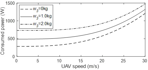
Figure 7: Propulsion power consumption (LABEL:eq:1) versus speed $v$ for different payload weights $w_{3}$.

Fig. 8 shows the UAV trajectory and the corresponding delivery time $T$ for our and benchmark algorithms.

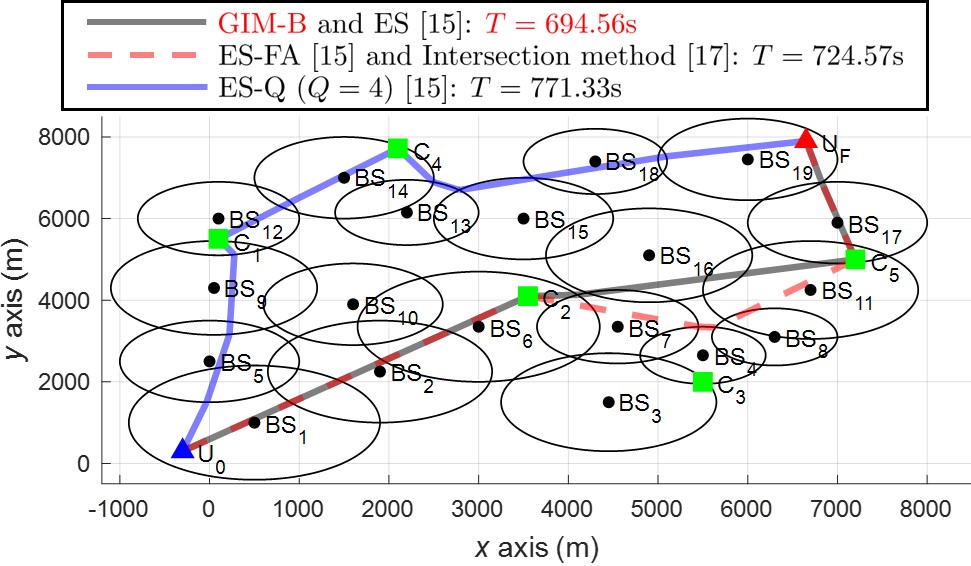
Figure 8: Comparison of trajectory and the corresponding delivery time $T$ for algorithms to solve Problem 1.

We note that the ES-FA algorithm [15] and intersection method [17] find the same trajectory, but different from the optimal trajectory of the ES algorithm [15] and our GIM-B algorithm. The ES-Q algorithm [15] with $Q=2$ cannot find any trajectory from $\mathbf{u}_{0}$ to $\mathbf{u}_{F}$ due to the battery constraint. The ES-Q algorithm with $Q=4$ has a higher complexity than our GIM-B algorithm because $QN>M$. However, it has a significant lower travel time $T$ even than the ES-FA and the intersection method algorithms, since it cannot derive a path $\mathbf{u}_{0}$ to $\mathbf{c}_{2}$ with the quantization points that the UAV can travel without battery replacement. Fig. 9 shows the optimal graph at the global level and the corresponding maximum possible speed $v_{\mathrm{max}}$ for each edge under the environment in Fig. 8. We can see that for each edge, the maximum travel speed $v_{\mathrm{max}}$ decreases as its travel distance increases.

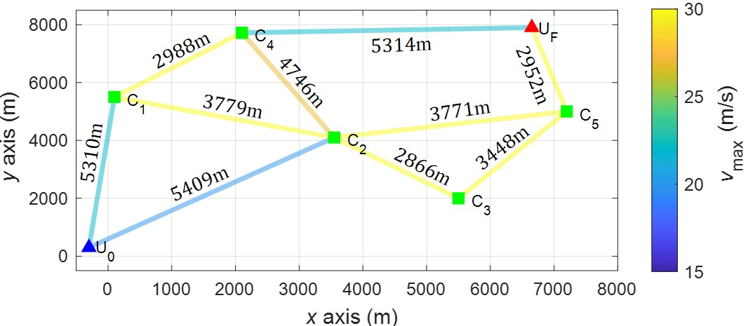
Figure 9: Optimal graph at the global level and the corresponding maximum possible speed $v_{\mathrm{max}}$ for each edge.

Fig. 10 compares the optimal UAV trajectory and the corresponding delivery time $T$ for different payload weight $w_{3}$, battery weight $w_{2}$, and delay $\tau_{C_{1}}$ at charging station $C_{1}$. We can see that the UAV avoids $C_{1}$ with the higher battery swapping delay $\tau_{C_{1}}=200\mathrm{s}$ (red), it visits more CSs with the larger payload weight $w_{3}=1.5\mathrm{kg}$ (blue), and it visits less CSs with the larger battery weight $w_{2}=1.2\mathrm{kg}$ (green).

Figure 10: Comparison of optimal trajectory and the corresponding delivery time $T$ for the cases that battery swapping delay $\tau_{C_{1}}=200\mathrm{s}$, payload weight $w_{3}=1.5\mathrm{kg}$, and battery weight $w_{2}=1.2\mathrm{kg}$.

In Fig. 11, the optimal delivery time $T$ is plotted for different battery swapping delays and payload weights $w_{3}\in[0:0.1:3.5]\mathrm{kg}$ under the same environment as in Fig. 10. We can verify that $T$ increases as the battery swapping delay and the payload weight increase and that the payload cannot be delivered from $\mathbf{u}_{0}$ to $\mathbf{u}_{F}$ if $w_{3}$ is too large, i.e., if it exceeds $2.8\mathrm{kg}$ under this setting.

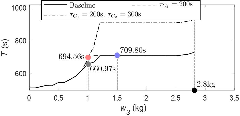
Figure 11: Payload weight $w_{3}$ versus optimal delivery time $T$ for different $\tau_{C_{1}}$ and $\tau_{C_{3}}$.

Fig. 12 compares the optimal delivery time $T$ for the case that the UAV can fly with a fixed speed of $v_{\mathrm{fix}}\in[15:1:30]\mathrm{m/s}$ (fixed speed) and for the case that it can change its speed in the speed set $\mathcal{V}$ (dynamic speed) under the same environment as in Fig. 10. Note that in the fixed speed case, the UAV chooses its speed in the set $\{0,v_{\mathrm{fix}}\}$. We can check that the dynamic speed case has a lower travel time than the fixed speed case for every $v_{\mathrm{fix}}\in[15:1:30]\mathrm{m/s}$ because the maximum allowable speed between each pair of CSs at the local level depends on its travel distance as shown in Fig. 9. In small battery weight $w_{2}=0.6\mathrm{kg}$, any trajectory from $u_{0}$ to $u_{F}$ cannot be derived in the fixed speed case with $v_{\mathrm{fix}}>22\mathrm{m/s}$ since flying at a high speed is not efficient in terms of the energy consumption as shown in Fig. 7.

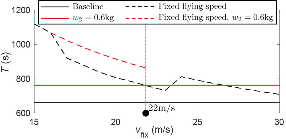
Figure 12: Flying speed $v_{\mathrm{fix}}$ versus optimal delivery time $T$ for the cases that the UAV can only fly with a fixed speed $v_{\mathrm{fix}}\in[15:1:30]\mathrm{m/s}$ and change its speed in the speed set $\mathcal{V}$.

Finally, Fig. 13 plots the maximum deliverable weight $w_{3}$ according to the battery weights $w_{2}\in[0.5:0.02:1]\mathrm{kg}$ for different unavailable CSs, where we say that charging station $C_{n}$ is unavailable if its battery swapping delay $\tau_{C_{n}}=\infty$. We can check that the maximum deliverable weight decreases as $w_{2}$ decreases and the number of unavailable CSs increases.

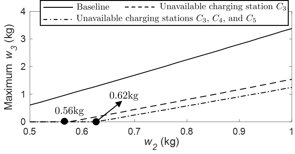
Figure 13: Battery weight $w_{2}$ versus maximum deliverable payload $w_{3}$ for different unavailable CSs.

VII Conclusion

For the problem of path planning for a cellular-enabled UAV with connectivity and battery constraints, the generalized intersection method with battery constraint (GIM-B) algorithm was proposed that computes an optimal path in polynomial time. Its effectiveness in terms of computational complexity and resultant mission completion time was demonstrated by comparing with previously proposed algorithms both in analytically and numerically. Furthermore, we proposed the bottleneck edge search method that finds the maximum deliverable payload weight under the connectivity and battery constraints. Various numerical results were presented to illustrate the effects of the environmental parameters on the optimal UAV path and the corresponding delivery time.

Let us conclude with some remarks on further works. We assumed that the delay at each CS is fixed over time, but in general it changes over time in practice. It would be interesting to consider the scenario with time-varying delays at charging stations and develop shortest path finding algorithms over time-dependent graphs [37, 38]. Another interesting scenario would be to consider more realistic coverage regions based on radio map taking into account signal blockage and reflection by buildings and interference from other BSs [39, 19].

References

- [1] H.-S. Im, K.-Y. Kim, and S.-H. Lee, “Trajectory optimization for cellular-enabled UAV with connectivity and battery constraints,” to be presented at IEEE Vehicular Technology Conference (VTC) 2023-Fall.
- [2] J. Zhang, J. F. Campbell, D. C. Sweeney II, and A. C. Hupman, “Energy consumption models for delivery drones: A comparison and assessment,” in Transportation Research Part D: Transport and Environment, vol. 90, 2021, p. 102668.
- [3] K. Kanistras, G. Martins, M. J. Rutherford, and K. P. Valavanis, “A survey of UAVs for traffic monitoring,” in 2013 International Conference on Unmanned Aircraft Systems, 2013, pp. 221–234.
- [4] M. Mozaffari, W. Saad, M. Bennis, Y.-H. Nam, and M. Debbah, “A tutorial on UAVs for wireless networks: Applications, challenges, and open problems,” in IEEE Communications Surveys and Tutorials, vol. 21, no. 3, 2019, pp. 2334–2360.
- [5] A. Al-Fuqaha, M. Guizani, M. Mohammadi, M. Aledhari, and M. Ayyash, “Internet of Things: A survey on enabling technologies, protocols, and applications,” in IEEE Communications Surveys and Tutorials, vol. 17, no. 4, 2015, pp. 2347–2376.
- [6] Y. Yu, J. Tang, J. Huang, X. Zhang, D. K. C. So, and K.-K. Wong, “Multi-objective optimization for UAV-assisted wireless powered IoT networks based on extended DDPG algorithm,” in IEEE Transactions on Communications, vol. 69, no. 9, 2021, pp. 6361–6374.
- [7] W. Shi, H. Zhou, J. Li, W. Xu, N. Zhang, and X. Shen, “Drone assisted vehicular networks: Architecture, challenges and opportunities,” in IEEE Network, vol. 32, no. 3, 2018, pp. 130–137.
- [8] A. Fotouhi et al., “Survey on UAV cellular communications: Practical aspects, standardization advancements, regulation, and security challenges,” in IEEE Communications Surveys and Tutorials, vol. 21, no. 4, 2019, pp. 3417–3442.
- [9] B. Li, Q. Li, Y. Zeng, Y. Rong, and R. Zhang, “3D trajectory optimization for energy-efficient UAV communication: A control design perspective,” in IEEE Transactions on Wireless Communications, vol. 21, no. 6, 2022, pp. 4579–4593.
- [10] Y. Zeng, J. Xu, and R. Zhang, “Energy minimization for wireless communication with rotary-wing UAV,” in IEEE Transactions on Wireless Communications, vol. 18, no. 4, 2019, pp. 2329–2345.
- [11] K. K. Nguyen, T. Q. Duong, T. Do-Duy, H. Claussen, and L. Hanzo, “3D UAV trajectory and data collection optimisation via deep reinforcement learning,” in IEEE Transactions on Communications, vol. 70, no. 4, 2022, pp. 2358–2371.
- [12] H. Qi, Z. Hu, H. Huang, X. Wen, and Z. Lu, “Energy efficient 3-D UAV control for persistent communication service and fairness: A deep reinforcement learning approach,” in IEEE Access, vol. 8, 2020, pp. 53 172–53 184.
- [13] A. Li, Q. Wu, and R. Zhang, “UAV-enabled cooperative jamming for improving secrecy of ground wiretap channel,” in IEEE Wireless Communications Letters, vol. 8, no. 1, 2019, pp. 181–184.
- [14] M. Cui, G. Zhang, Q. Wu, and D. W. K. Ng, “Robust trajectory and transmit power design for secure UAV communications,” in IEEE Transactions on Vehicular Technology, vol. 67, no. 9, 2018, pp. 9042–9046.
- [15] S. Zhang, Y. Zeng, and R. Zhang, “Cellular-enabled UAV communication: A connectivity-constrained trajectory optimization perspective,” in IEEE Transactions on Communications, vol. 67, no. 3, 2019, pp. 2580–2604.
- [16] S. Zhang and R. Zhang, “Trajectory design for cellular-connected UAV under outage duration constraint,” in 2019 IEEE International Conference on Communications, 2019, pp. 1–6.
- [17] Y.-J. Chen and D.-Y. Huang, “Trajectory optimization for cellular-enabled UAV with connectivity outage constraint,” in IEEE Access, vol. 8, 2020, pp. 29 205–29 218.
- [18] O. Esrafilian, R. Gangula, and D. Gesbert, “3D-map assisted UAV trajectory design under cellular connectivity constraints,” in 2020 IEEE International Conference on Communications, 2020, pp. 1–6.
- [19] S. Zhang and R. Zhang, “Radio map-based 3D path planning for cellular-connected UAV,” in IEEE Transactions on Wireless Communications, vol. 20, no. 3, 2021, pp. 1975–1989.
- [20] A. Chapnevis, İ. Güvenç, L. Njilla, and E. Bulut, “Collaborative trajectory optimization for outage-aware cellular-enabled UAVs,” in 2021 IEEE 93rd Vehicular Technology Conference, 2021, pp. 1–6.
- [21] Y. Zeng and X. Xu, “Path design for cellular-connected UAV with reinforcement learning,” in 2019 IEEE Global Communications Conference, 2019, pp. 1–6.
- [22] B. Khamidehi and E. S. Sousa, “A double Q-learning approach for navigation of aerial vehicles with connectivity constraint,” in 2020 IEEE International Conference on Communications, 2020, pp. 1–6.
- [23] Y. Zeng, X. Xu, S. Jin, and R. Zhang, “Simultaneous navigation and radio mapping for cellular-connected UAV with deep reinforcement learning,” in IEEE Transactions on Wireless Communications, vol. 20, no. 7, 2021, pp. 4205–4220.
- [24] X. Wang and M. C. Gursoy, “Learning-based UAV trajectory optimization with collision avoidance and connectivity constraints,” in IEEE Transactions on Wireless Communications, vol. 21, no. 6, 2022, pp. 4350–4363.
- [25] Y.-J. Chen and D.-Y. Huang, “Joint trajectory design and BS association for cellular-connected UAV: An imitation-augmented deep reinforcement learning approach,” in IEEE Internet of Things Journal, vol. 9, no. 4, 2022, pp. 2843–2858.
- [26] K. Sundar and S. Rathinam, “Algorithms for routing an unmanned aerial vehicle in the presence of refueling depots,” in IEEE Transactions on Automation Science and Engineering, vol. 11, no. 1, 2014, pp. 287–294.
- [27] B. N. Coelho et al., “A multi-objective green UAV routing problem,” in Computers and Operations Research, vol. 88, 2017, pp. 306–315.
- [28] M. Fan et al., “Deep reinforcement learning for UAV routing in the presence of multiple charging stations,” in IEEE Transactions on Vehicular Technology, vol. 72, no. 5, 2023, pp. 5732–5746.
- [29] M. Y. Arafat and S. Moh, “JRCS: Joint routing and charging strategy for logistics drones,” in IEEE Internet of Things Journal, vol. 9, no. 21, 2022, pp. 21 751–21 764.
- [30] A. Al-Hourani, S. Kandeepan, and S. Lardner, “Optimal LAP altitude for maximum coverage,” in IEEE Wireless Communications Letters, vol. 3, no. 6, 2014, pp. 569–572.
- [31] A. Al-Hourani, S. Kandeepan, and A. Jamalipour, “Modeling air-to-ground path loss for low altitude platforms in urban environments,” in 2014 IEEE Global Communications Conference, 2014, pp. 2898–2904.
- [32] P. K. Agyapong, M. Iwamura, D. Staehle, W. Kiess, and A. Benjebbour, “Design considerations for a 5G network architecture,” in IEEE Communications Magazine, vol. 52, no. 11, 2014, pp. 65–75.
- [33] R. S. Sutton and A. G. Barto, Reinforcement learning: An introduction. Cambridge, MA, USA: A Bradford Book, 2018, vol. 2.
- [34] D. Lee, J. Zhou, and W. T. Lin, “Autonomous battery swapping system for quadcopter,” in 2015 International Conference on Unmanned Aircraft Systems, 2015, pp. 118–124.
- [35] E. W. Dijkstra, “A note on two problems in connection with graphs.” in Numerische Mathematik, vol. 1, 1959, pp. 269–271.
- [36] D. B. West, Introduction to graph theory. New Jersey, USA: Prentice Hall, 2001, vol. 2.
- [37] A. Orda and R. Rom, “Shortest-path and minimum-delay algorithms in networks with time-dependent edge-length,” in Journal of the Association for Computing Machinery, vol. 37, no. 3, 1990, p. 607–625.
- [38] B. Ding, J. X. Yu, and L. Qin, “Finding time-dependent shortest paths over large graphs,” in Proceedings of the 11th International Conference on Extending Database Technology: Advances in Database Technology, 2008, p. 205–216.
- [39] J. Chen, U. Yatnalli, and D. Gesbert, “Learning radio maps for UAV-aided wireless networks: A segmented regression approach,” in 2017 IEEE International Conference on Communications, 2017, pp. 1–6.