- Supplementary Material -
Mesh Density Adaptation for
Template-based Shape Reconstruction

In this supplementary document, we provide technical details, additional discussion, and more visual results. In Sec. 1, we provide more information on the hyperparameters for the experiments conducted in the main paper. In Sec. 2, we provide an additional experiment and discussion on the behavior of diffusion re-parameterization in the context of density adaptation. In Secs. 3 and 4, we provide additional visual results for inverse rendering and non-rigid registration, respectively. Sec. 5 provides visual results for the limitation.

1. Implementation Details

1.1. Inverse Rendering

Given adaptation strength $m$ and the number of total iterations $T$, the scheduling for the weights $w_{u}$ and $w_{k}$ of our adaptation energies at the $t$-th iteration is defined as

(1) $$\begin{split}w_{u}&=\begin{cases}m&\text{ if }\frac{t}{T}<\frac{1}{4}\\ 0&\text{ otherwise}\\ \end{cases}\\ w_{k}&=\begin{cases}2m&\text{ if }\frac{1}{4}\leq\frac{t}{T}<\frac{1}{2}\\ 0&\text{ otherwise}.\\ \end{cases}\end{split}$$

The adaptation strength per reconstructed object is presented in Table 1.

The weights for Laplacian regularizations differ per reconstructed object. We reuse the regularization weights used for the comparison in (Nicolet et al., 2021). We list the values for the Laplacian regularizations in Table 2.

For (Nicolet et al., 2021) and ours, we use $\lambda=19$. Our method shares the same number of iterations as (Nicolet et al., 2021) using the UniformAdam optimizer in (Nicolet et al., 2021) with the same learning rate. Both (Nicolet et al., 2021) and ours do not employ learning late decay, so small high-frequency shakes around the end of the optimization may occur (see the supplementary video). We list the number of total iterations and learning rate per object in Table 3. The regularization weights and learning rates per example in Table 2 and Table 3 are set to the same values as in (Nicolet et al., 2021).

Table 1. Adaptation strength used for Ours in our experiments on inverse rendering

T-shirt	Suzanne	Bunny	Cranium	Plank	Bob
0.5	1.8	2.0	2.7	0.7	0.7

Table 2. Regularization weights used for the compared Laplacian regularizations in our experiments on inverse rendering.

	T-shirt	Suzanne	Bunny	Cranium	Plank	Bob
Laplacian	12	2.8	3.8	0.21	3.8	0.67
Bi-Laplacian	12	3.8	2.1	0.16	5.0	0.37

1.2. Non-rigid Surface Registration

Template mesh fitting

For our result, we use the same weight scheduling for density adaptation as in the inverse rendering. We fix $m=1.5$ and the number of total iterations $T=1400$. For both Ours and DR, diffusion re-parameterization without density adaptation, we use $\lambda=19$.

Landmark resampling

In the alignment of landmarks on sphere, we use a diagonal weight matrix

(2) $$\mathbf{W}_{ii}=\begin{cases}1.0\times 10^{4}&\text{ if }i=16\\ 1&\text{ otherwise},\end{cases}$$

where $16$ is the index for the landmark on the tip of the nose. The total number of landmarks is $38$. The landmarks for the artist-sculpted meshes are obtained from 3DCaricShop (Qiu et al., 2021). We used all faces in 3DCaricShop to perform the landmark resampling.

Table 3. Number of iterations and learning rate for the inverse rendering experiment.

	T-shirt	Suzanne	Bunny	Cranium	Plank	Bob
# input views	16	13	16	16	16	16
# iter (Laplacian & Bi-Laplacian)	390	1130	1450	1910	960	940
# iter (Ours & (Nicolet et al., 2021))	370	1080	1380	5000	1500	930
learning rate	3E-3	2E-3	1E-2	5E-3	3e-3	3e-3

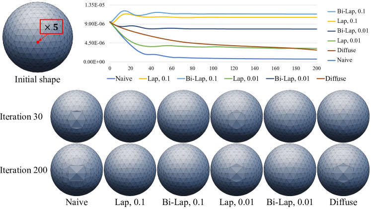
Figure 1. The behavior of different regularizations. We show the results of minimizing our adaptation energy with $\mathbf{l}^{\prime}$ constructed by multiplying the mean edge length of one vertex by five. $\mathbf{p}$ is constrained to be on a sphere. (Naive) Without any regularization, the update is instant, and the error is minimized in a short time. (Lap, Bi-Lap) Results with Laplacian or Bi-Laplacian energy with two different weights are shown. These regularizations conflict with our goal of adapting the mesh density, so giving high weight ends up with non-adjustment of the density. Using a smaller weight, Lap_0.01 allows the adaptation of mesh density but results in a quick update at almost same rate as the Naive case. (Diffuse) (Nicolet et al., 2021) does not conflict with density adaptation and prioritizes smooth deformation in the early stage, showing gradual decrease in the error and the eventual error minimization.

1.3. Running time

Our density adaptation term increases the optimization time by 10-15%. In inverse rendering, (Nicolet et al., 2021) takes 28 seconds and ours takes 32 seconds on average to reconstruct the shape of one instance. In non-rigid registration, the optimization takes 19 seconds without density adaptation and takes 22 seconds with our density adaptation.

2. Behavior of diffusion re-parameterization

Diffusion re-parameteterization helps density adaptation by stabilizing the optimization. Our density adaptation is based on the examination of Laplacian of intermediate results. However, because Laplacian is sensitive to local shape change, the intermediate results may contain noisy Laplacian. So, the adjustment in the density based on the Laplacian should not be instant. Quick fluctuations from instant adjustment may induce unstable optimization.

Diffusion re-parameterization generally prefers smooth deformation but eventually allows adjustment of regularity if the gradients are accumulated enough. This slow-starting but eventually-achieving behavior is presented in Fig. 1. In this sense, we find diffusion re-parameterization is an appropriate smoothness regularization for our method because it prevents quick fluctuations in the density adjustment while not conflicting with our goal.

3. Additional Results for Inverse Rendering

We provide more results for inverse rendering in Fig. 2. We show the results of (Nicolet et al., 2021) and ours using the same template mesh. Fig. 5 further visualizes the progression of optimization over time. Reported photometric mean absolute error (MAE) values are averaged using the results from scenes of Suzanne, Cranium, Bob, Bunny, T-shirt, and Plank. The weight scheduling for the density adaptation term increases the error of our method at 25% iteration mark, but due to better vertex density from the adaptation, our method results in the lowest error in the end.

4. Additional results for non-rigid registration

Fig. 3 presents more results from our non-rigid registration on the artist-sculpted 3D meshes in (Qiu et al., 2021). Our non-rigid registration using the sphere template mesh with automatically annotated landmarks produces more accurate reconstructions.

Template landmarks may hinder vertex relocation needed for density adaptation, as shown in Fig. 6. Configuration of landmarks affects the resulting mesh density; vertices would not freely relocate around landmarks because the energy term for the landmarks in the optimization pins the 3D coordinates of landmark vertices on the template. So, compared to without-landmark fitting, fitting with landmarks may exhibit sparser density in some regions. This side effect can be avoided by fitting with a fewer number of landmarks or without landmarks.

Using the dense correspondence obtained from our non-rigid registration, texture maps can be shared between the registration results, enabling texture transfer. We show texture transfer results in Fig. 4.

5. Limitations

Fig. 7 visualizes the limitation of our density adaptation based on Laplacian calculation from intermediate optimization results. While our proposed algorithm for calculating desired mesh density handles large structures well, fine details on flat region may not be benefited from the increase in density for better reconstruction.

(Nicolet et al., 2021)

Ours

GT

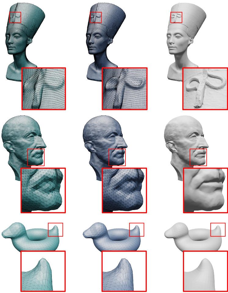
Figure 2. Additional visual results for inverse rendering.

GT                            Ours                  (Qiu et al., 2021)

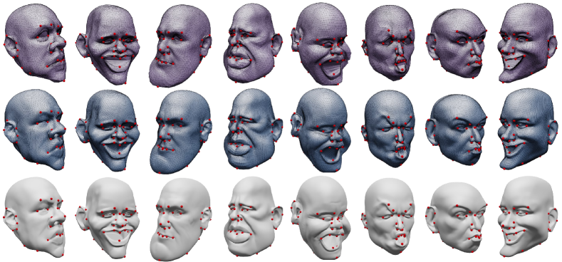
Figure 3. Additional visual results of non-rigid registration.

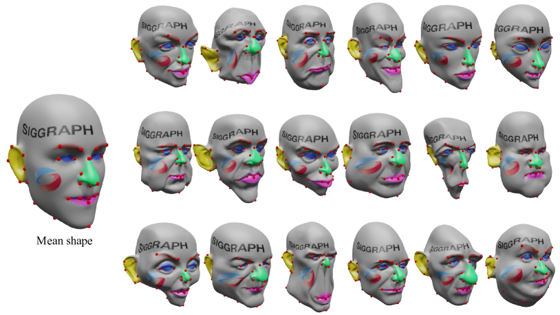
Figure 4. Texture transfer results using dense correspondences obtained from our non-rigid registration.

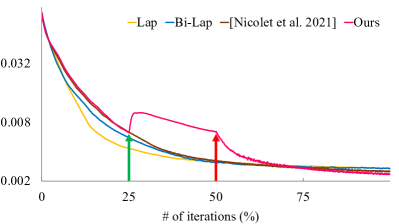
Figure 5. Progression of energy (MAE) over iterations in the inverse rendering experiment. Average energy is shown at each percentile. The Y axis is log-scaled using base $4$. In ours, introducing non-zero $w_{k}$ at 25% increases the energy (green arrow), but by setting $w_{u}=0$ and $w_{k}=0$ after 50% (red arrow), ours ends up with the lowest energy due to improved mesh density.

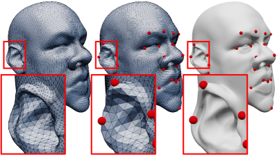
Ours w/o lmk               Ours w/ lmk                        GT

Figure 6. Side-effect of using template landmarks. In some instances, using our template landmarks may hinder vertex relocation.

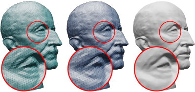
Figure 7. Limitations. The vertex density for fine-scale details on a flat region may not increase. Large extruded regions are manifested early in the iterative optimization, so our density adaptation attracts vertices to such regions. In this example, the density around the extruded chin is increased, but the density increase is accompanied by decreases in the density of other regions, such as the eyes. Fine details manifest late in the optimization, so vertices may not be strongly attracted to them. Left: Without density adaptation. Middle: With density adaptation. Right: Ground truth.

References

- (1)
- Nicolet et al. (2021) Baptiste Nicolet, Alec Jacobson, and Wenzel Jakob. 2021. Large steps in inverse rendering of geometry. ACM Trans. Graph. 40, 6 (2021), 1–13.
- Qiu et al. (2021) Yuda Qiu, Xiaojie Xu, Lingteng Qiu, Yan Pan, Yushuang Wu, Weikai Chen, and Xiaoguang Han. 2021. 3dcaricshop: A dataset and a baseline method for single-view 3d caricature face reconstruction. In Proc. CVPR. 10236–10245.