UPFL: Unsupervised Personalized Federated Learning towards New Clients

Abstract.

Personalized federated learning has gained significant attention as a promising approach to address the challenge of data heterogeneity. In this paper, we address a relatively unexplored problem in federated learning. When a federated model has been trained and deployed, and an unlabeled new client joins, providing a personalized model for the new client becomes a highly challenging task. To address this challenge, we extend the adaptive risk minimization technique into the unsupervised personalized federated learning setting and propose our method, FedTTA. We further improve FedTTA with two simple yet effective optimization strategies: enhancing the training of the adaptation model with proxy regularization and early-stopping the adaptation through entropy. Moreover, we propose a knowledge distillation loss specifically designed for FedTTA to address the device heterogeneity. Extensive experiments on five datasets against eleven baselines demonstrate the effectiveness of our proposed FedTTA and its variants. The code is available at: https://github.com/anonymous-federated-learning/code.

1. Introduction

Federated learning (FL) is a popular machine learning paradigm, in which multiple clients collaboratively train machine learning models without compromising their data privacy (Kairouz et al., 2021). During each FL communication round, the server synchronizes the latest global model with a subset of selected clients. These selected clients then optimize the model on their local data and send back the updated model parameters to the server. The server then aggregates the received model parameters and updates the global model.

Data heterogeneity often poses a significant challenge to FL, where the data distribution among clients is non-independent and non-identically distributed (non-IID). This non-IID nature of the data may significantly impact the model performance. To address this challenge, personalized federated learning has emerged as a promising approach, as it allows for a personalized model for each participating client (Arivazhagan et al., 2019; Fallah et al., 2020; Shamsian et al., 2021). Most of the works focus on improving the performance of the global model by tailoring it to the specific data distribution of each client, while few works have considered how to provide personalized models for clients that are not available during training time, i.e., new clients. Per-FedAvg (Fallah et al., 2020) and pFedHN (Shamsian et al., 2021) have made some explorations, which personalize the model for new clients by fine-tuning on their labeled datasets. However, during inference time, new clients often lack labeled data, which motivates us to investigate the unsupervised settings.

In this paper, we consider a practical yet more challenging task for heterogeneous federated learning: Unsupervised Personalized Federated Learning towards new clients (UPFL). Specifically, after a federated model has been trained and deployed, new clients may wish to join and utilize the deployed model for inferring their local unlabeled datasets. The data distribution of these new clients might significantly differ from that of the training clients. Providing personalized models for these new clients with only unlabeled datasets is a highly challenging task. To the best of our knowledge, the only work that addresses the same task as ours is ODPFL-HN (Amosy et al., 2021) , which extends pFedHN to the UPFL setting. Specifically, ODPFL-HN trains an encoder network to learn a representation for each client based on its unlabeled data, and then feeds the client representation to a hypernetwork that generates a personalized model for that client. However, ODPFL-HN involves additionally transmitting the client representation, which could potentially put the clients’ privacy at risk. And it would generate the same model structure for all clients, which limits its applicability in heterogeneous FL settings.

To effectively address the above-mentioned UPFL task, we leverage the idea of adaptive risk minimization (Zhang et al., 2021c) into federated learning and propose our approach FedTTA. Specifically, each client $c_{i}$ meta-learns a base prediction model $f(\cdot|\psi^{i})$ and an adaptation model $g(\cdot|\phi^{i})$, which takes in the outputs of $f(\cdot|\psi^{i})$ on unlabeled data points and produces personalized parameters $\tilde{\psi^{i}}$. The server aggregates the base prediction models and adaptation models from the clients to update the server base prediction model $\psi^{s}$ and adaptation model $\phi^{s}$. When a new client with unlabeled data joins, it downloads the server models $\psi^{s}$ and $\phi^{s}$, and adapts $\psi^{s}$ to a personalized one $\tilde{\psi^{s}}$ under the supervision of $\phi^{s}$.

We further introduce an improved version of FedTTA, denoted as FedTTA++, which leverages two simple yet effective optimization strategies: (1) enhancing the adaptation model’s personalization capability with regularization on the base prediction model and (2) early stopping the adaptation during testing based on the entropy of the prediction model’s outputs. First, the base prediction model in FL can easily overfit due to local data scarcity. Moreover, a highly personalized base prediction model could already perform very well on the local dataset, making it difficult for the adaptation model to learn the ability to customize the base prediction model. To address this, we introduce regularization on the outputs of the base prediction model to enhance the training of the adaptation model’s personalization capability. Second, we observe that only one-step update may result in an under-explored personalization model, while excessively updating the base prediction model during adaptation can lead to sub-optimal solutions. To address this, we propose to utilize the entropy of the personalized model’s predictions as an unsupervised metric for early stopping of the adaptation process, as personalized models generally exhibit low entropy in their predictions. Specifically, we stop the adaptation when the entropy of the personalized model’s predictions does not decrease within a certain steps.

Moreover, device heterogeneity is also prevalent in federated learning, with clients exhibiting varying computing and storage capabilities, thereby resulting in model structures and sizes that differ significantly. To address device heterogeneity, we develop a heterogeneous version of FedTTA, called HeteroFedTTA, based on a classic heterogeneous federated learning framework FedMD (Li and Wang, 2019) that enables knowledge transfer between heterogeneous clients through knowledge distillation. Based on FedTTA, a straightforward approach is to distill knowledge for student’s base prediction model and adaptation model in an end-to-end manner, with the aim of approximating the predictions of the student’s personalized model to those of the teacher. However in FedTTA, the knowledge from teacher model may arise from two sources: the general prediction capability of the base prediction model and the adaptation capability of the adaptation model in transforming a base prediction model into a personalized one. Thus, we suggest a novel knowledge distillation loss that enforces the student’s base prediction model and adaptation model to learn from the corresponding models of the teacher, respectively.

We summarize our contributions as follows:

• We address a practical and yet rarely studied task in federated learning, namely UPFL, where the primary challenge is to personalize models for new unlabeled clients. To address this challenge, we propose FedTTA.

• We further propose FedTTA++, an enhanced version of FedTTA, which leverages two simple optimization strategies to achieve remarkable performance improvements.

• Considering the heterogeneous model setting and the unique architecture of FedTTA, we suggest a novel knowledge distillation loss, which is empirically shown to be effective.

• We conduct extensive experiments on five benchmark datasets against eleven baselines to evaluate the effectiveness of our proposed methods, and the results demonstrate their efficacy in addressing the UPFL task.

2. Related Work

Personalized federated learning (PFL) customizes each client with a personalized model based on its local data (Arivazhagan et al., 2019; Fallah et al., 2020; Shamsian et al., 2021). PFL has gained significant advancements recently. For example, FedPer (Arivazhagan et al., 2019) learns a universal representation layer across clients and personalizes a local model with a unique classification head. pFedHN (Shamsian et al., 2021) leverages hyper-network to output a personalized model for each client, and Per-FedAvg (Fallah et al., 2020) coordinates clients to learn a global model, from which each client can quickly adapt to a personalized model through a one-step update. Most existing PFL methods focus solely on improving the performance of training clients, neglecting the crucial aspect of generalization to new clients. Although pFedHN and Per-FedAvg have made some attempts to address this, both of them rely on fine-tuning on new clients’ labeled datasets, which does not apply to our task.

Generalized federated learning (GFL) is proposed to enhance the performance of new clients by learning invariant mechanisms among training clients and expecting them to generalize well to new clients (Tenison et al., 2022; Nguyen et al., 2022; Liu et al., 2021a; Zhang et al., 2021b; Caldarola et al., 2022; Qu et al., 2022). For example, FedGMA (Tenison et al., 2022) presents a gradient-masked averaging approach to better capture the invariant mechanism across heterogeneous clients. FedSR (Nguyen et al., 2022) implicitly aligns the marginal and conditional distribution of the representation with two regularizers. A similar idea has also been exploited in FedADG (Zhang et al., 2021b), which adaptively learns a dynamic reference distribution to accommodate all source domains. GFL methods output a single model and directly apply it to test clients, while FedTTA  is an unsupervised PFL method that adapts the base prediction model to a personalized model based on hints from the new client’s unlabeled dataset. To the best of our knowledge, ODPFL-HN (Amosy et al., 2021) is the only work that addresses the same problem as ours. ODPFL-HN trains a client encoder network and a hypernetwork, where the client encoder network encodes an unlabeled client to a representation and the hypernetwork generates a personalized model based on that representation.

Test-Time Adaptation (TTA) refers to fine-tuning a model during inference time to adapt to specific test data. TTA was first introduced by Test-Time Training (TTT) (Sun et al., 2020), which additionally learns a self-supervised auxiliary task (rotation prediction) during training and fine-tunes the feature encoder based on this task during testing. Since then, test-time adaptation methods have been proposed one after another. For example, TTT++ (Liu et al., 2021b) builds upon TTT and introduces a test-time feature alignment strategy. TENT (Wang et al., 2020) fine-tunes the model at inference time to optimize the model confidence by minimizing the entropy of its predictions. However, there has been limited exploration of the intersection of personalized federated learning and test-time adaptation. The recently proposed work, FedTHE (Jiang and Lin, 2022), studies the problem that clients’ local test sets evolve during deployment and proposes to robustify federated learning models by adaptive ensembling of the global generic and local personalized classifier of a two-head federated learning model. This approach does not apply to our setting, as new clients lack personalized classifiers.

Knowledge Distillation (KD) has been receiving increasing attention from the federated learning community, as it enables the aggregation of knowledge from heterogeneous models (Gao et al., 2022). Existing heterogeneous federated learning methods typically aggregate the logits of clients rather than their model parameters on the server. Each client then updates the local model to approximate the global average logits. For instance, FedMD (Li and Wang, 2019) performs ensemble distillation on a public dataset, while KT-pFL (Zhang et al., 2021a) improves on FedMD by updating the local model with the personalized logits of each client through a parameterized knowledge coefficient matrix. However, our focus in this paper is not on the heterogeneous federated learning framework. Instead, our contribution is proposing a more effective knowledge distillation loss, which can better facilitate the distillation of the models in FedTTA.

3. Methodology

In this section, we will provide a detailed description of the learning setting of UPFL towards new clients. We will then introduce our proposed method FedTTA and propose an enhanced version FedTTA++ , which leverages two simple optimization strategies: enhancing the training of the adaptation model by regularizing the outputs of the base prediction model and early stopping the adaptation process during testing through entropy. We will also give a heterogeneous version of FedTTAbased on FedMD, denoted as HeteroFedTTA. We suggest a novel knowledge distillation loss for HeteroFedTTA, which facilitates the application of FedTTA in heterogeneous federated learning setting.

3.1. Problem Formulation

In this work, we focus on the scenario where training is performed on $N$ clients, denoted by $\{c_{1},\cdots,c_{N}\}$, each with a private dataset $\mathcal{D}_{i}=\{(x_{j}^{(i)},y_{j}^{(i)})\}_{j=1}^{m_{i}}$ of size $m_{i}$, and new clients may join in at the inference stage. Our objective is to learn an unsupervised adaptation strategy from the training clients, which can provide a personalized model for a new client based on its unlabeled dataset $\mathcal{D}_{new}=\{x_{j}^{(i)}\}_{j=1}^{m_{new}}$. We refer to this learning setting as the Unsupervised Personalized Federated Learning (UPFL) .

3.2. Algorithm FedTTA

The proposed framework is illustrated in Fig. 1. It can be seen from the figure that each client’s local models consist of two components: base prediction model $f(\cdot;\psi)$ and adaptation model $g(\cdot;\phi)$. The base prediction model $f$ is the task network for classification, which takes a batch of samples $X:=\{x_{1},\cdots,x_{B}\}$ and outputs the corresponding logits $Z:=\{z_{1},\cdots,z_{B}\}$  :

(1) $$Z=f(X,\psi)$$

The adaptation model $g$ is responsible for customizing the base prediction model to a personalized prediction model. $g$ takes the outputs of the base prediction model and outputs a scalar for each sample that measures how poorly current base prediction model $f$ performs on corresponding unlabeled data. Following (Zhang et al., 2021c), we use the $\ell_{2}$-norm of these scalars across the batch as the personalization loss of $f$ on the client. Adaptation is performed by updating $f(\cdot;\psi)$ towards minimizing the personalization loss. Specifically,

(2) $$\ell_{per}=\|g(Z;\phi)\|_{2}$$

Obviously, the output of the adaptation model is independent of samples order. Regardless of how the samples are sorted, the adaptation model’s evaluation of the base prediction model’s performance is consistent.

3.2.1. Training Phase

During training, each client has access to its labeled dataset $\mathcal{D}_{i}:=\{(x_{j}^{(i)},y_{j}^{(i)})\}_{j=1}^{m_{i}}$. We denote $X_{i}:=\{x_{j}^{(i)}\}_{j=1}^{m_{i}}$ and $Y_{i}:=\{y_{j}^{(i)}\}_{j=1}^{m_{i}}$. We simulate the testing environment to meta-train the base prediction model and the adaptation model. Specifically, we first adapt the base prediction model towards a personalized model:

(3) $$Z_{i}=f({X}_{i};\psi^{i})$$

(4) $$\ell_{per}=\|g(Z_{i};\phi^{i})\|_{2}$$

(5) $$\tilde{\psi}^{i}\leftarrow\psi^{i}-\eta_{inner}\nabla_{\psi}\ell_{per},$$

where $\eta_{inner}$ is the learning rate of the prediction model in the inner loop. Then, we optimize the parameters $\psi^{i}$ and $\phi^{i}$ to minimize the loss of the personalized model $\tilde{\psi}^{i}$ on its local dataset:

(6) $$\tilde{Z_{i}}=f({X}_{i};\tilde{\psi}^{i})$$

(7) $$\mathcal{L}=\ell_{CE}(\tilde{Z_{i}};Y_{i})$$

(8) $$\psi^{i}\leftarrow\psi^{i}-\eta_{outer}\nabla_{\psi}\mathcal{L}$$

(9) $$\phi^{i}\leftarrow\phi^{i}-\eta_{adapt}\nabla_{\phi}\mathcal{L},$$

where $\eta_{outer}$ is the learning rate of the prediction model in the outer loop and $\eta_{adapt}$ denotes the learning rate of the adaptation model.

3.2.2. Testing Phase

Once a new client $c_{new}$ joins after the federated model has been deployed, it downloads the models from the server and adapts the base prediction model under the supervision of the adaptation model, and then makes predictions based on the personalized prediction model:

(10) $$Z_{new}=f(\mathcal{D}_{new};\psi^{new})$$

(11) $$\psi^{new}\leftarrow\psi^{new}-\eta_{inner}\nabla_{\psi}\|g(Z_{new};\phi^{new})\|_{2}$$

(12) $$\tilde{Z}_{new}=f(\mathcal{D}_{new};\psi^{new})$$

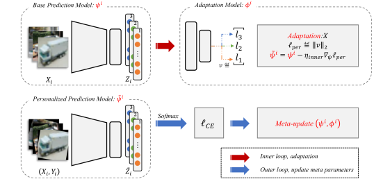
Figure 1. The figure depicts the local training process of client $c_{i}$ in FedTTA. The inner loop outputs a personalized prediction model, while the outer loop evaluates this model and meta-updates both the base prediction model and adaptation model accordingly.

3.3. Improved FedTTA (FedTTA++)

3.3.1. Enhance Adaptation Model with Regularization

In federated learning, the client data is often limited, which can easily lead to overfitting of the base prediction model. A highly personalized base prediction model can already perform very well on the client’s local data, making it difficult for the adaptation model to learn how to customize a general prediction model to a personalized prediction model. In addition, during testing, the base prediction model often gives general prediction results. Therefore, we expect the adaptation model to focus more on the general prediction model. Overfitting of the base prediction model can lead to poor generalization of the adaptation model. To mitigate the issue, during local training, we constrain the outputs of the local base prediction model to approach that of the server prediction model $\dot{Z}:=f(X_{i};\psi^{s})$, which enables the adaptation model to be effectively trained to adapt a general prediction model into a personalized one. We call such a variant of FedTTA as FedTTA-Prox. With the constraint, the loss function in Eq. 7 becomes:

(13) $$\mathcal{L}=\ell_{CE}(\tilde{Z_{i}};Y_{i})+\mu\ell_{KL}(\sigma(Z_{i})||\sigma(\dot{Z_{i}}))$$

, where $\ell_{KL}$ and $\sigma(\cdot)$ denote the KL divergence and softmax function, respectively, while $\mu$ serves as a balancing coefficient.

Different from FedProx (Li et al., 2020), which limits the local updates directly in parameter space for mitigating client variances, we regularize the base prediction model’s outputs (logits) to be general (less personalized) and expect the adaptation model can adjust them to be personalized ones.

3.3.2. Early Stop Adaptation through Entropy

FedTTA outputs a base prediction model and an adaptation model, aiming to personalize the base prediction model quickly for a new client through a one-step update under the adaptation model’s supervision. However, a one-step update may not be sufficient, and multi-step fine-tuning can often yield a better personalized model. We run FedTTA on CIFAR-10 dataset, and during testing, each client updates the base prediction model for 50 iterations. Interestingly, we have empirically observed a slight mismatch between $\ell_{per}$ (defined in Eq. 2) and the performance of the personalized model as fine-tuning progresses. The example in Fig. 2 shows that additional fine-tuning can improve the personalized model in the first 11 steps, but excessive fine-tuning can lead to a suboptimal personalized model. Obviously the number of fine-tuning steps is a crucial parameter that could vary among clients, and it is unreasonable to apply a universal hyperparameter to all clients.

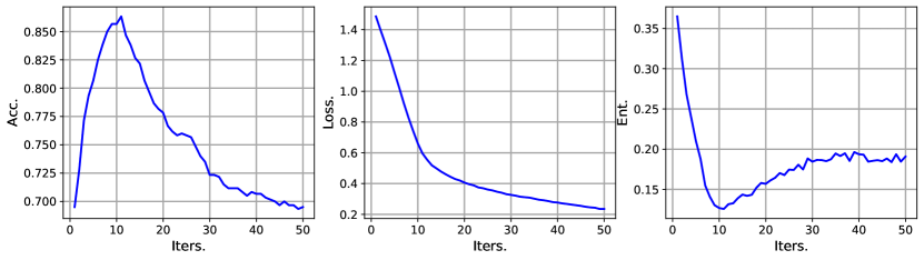
Figure 2. An example of mismatch between $\ell_{per}$ and the performance of the personalized prediction model. The figures show during adaptation a client’s change curves of the personalized prediction model’s accuracy (left), $\ell_{per}$ (middle), and the entropy of the personalized model’s predictions (right). While additional fine-tuning can improve the personalized model in the initial stages, excessive fine-tuning can lead to a suboptimal personalized model. To prevent this, we suggest early stopping the adaptation process when the entropy reaches its lowest point (at the 12-th iteration).

To address this, we suggest an adaptive early stopping strategy based on the entropy of the personalized model’s predictions. In general, a better personalized model will produce a more confident prediction with low entropy. Thus, we calculate the entropy of the personalized model’s predictions during fine-tuning and terminate fine-tuning when the entropy does not decrease within a certain steps. For example, we should stop the adaptation at the 12-th iteration for the client illustrated in Fig 2.

Input: initial parameters of base prediction model $\psi^{0}$ and adaptation model $\phi^{0}$, total communication rounds $R$, local iterations $\tau$, local minibatch size $B$, number of participating clients per round $M$, and maximum number of iterations for fine-tuning during testing $E$

Output: $\psi_{R}$ and $\phi_{R}$

[Training]

for each round $r$ : 0 to $R-1$ do

       Select a set of clients $\mathcal{S}_{r}$ of size $M$

       for each client $c_{i}\in\mathcal{S}_{r}$ do

             // Local Training

             $\{\psi^{i},\phi^{i}\}\leftarrow\{\psi_{r},\phi_{r}\}$

             $\mathcal{B}_{i}\leftarrow$ Split local dataset $\mathcal{D}_{i}$ into batches of size $B$

             for each iteration $t$ : 1 to $\tau$ do

                   Sample a batch $(X_{t},Y_{t})\sim\mathcal{B}_{i}$

                   $\dot{Z_{t}}=f(X_{t};\psi_{r})$

                   $Z_{t}=f(X_{t};\psi^{i})$

                   $\ell_{per}=\|g(Z_{t};\phi^{i})\|$

                   $\tilde{\psi}^{i}\leftarrow\psi^{i}-\eta_{inner}\nabla_{\psi}\ell_{per}$

                   $\tilde{Z_{t}}=f(X_{t};\tilde{\psi}^{i})$

                   $\mathcal{L}=\ell_{CE}(\tilde{Z_{t}};Y_{t})+\mu\ell_{KL}(\sigma(Z_{t})||\sigma(\dot{Z_{t}}))$

                   $\psi^{i}\leftarrow\psi^{i}-\eta_{base}\nabla_{\psi}\mathcal{L}$

                   $\phi^{i}\leftarrow\phi^{i}-\eta_{adapt}\nabla_{\phi}\mathcal{L}$

                  

             end for

            $\{\psi_{r+1}^{i},\phi_{r+1}^{i}\}\leftarrow\{\psi^{i},\phi^{i}\}$

             Client $c_{i}$ sends $\psi_{r+1}^{i}$ and $\phi_{r+1}^{i}$ back to server

            

       end for

      // Server Aggregation

       $\psi_{r+1}\leftarrow\frac{1}{M}\sum_{c_{i}\in\mathcal{S}_{r}}\psi_{r+1}^{i}$

       $\phi_{r+1}\leftarrow\frac{1}{M}\sum_{c_{i}\in\mathcal{S}_{r}}\phi_{r+1}^{i}$

      

end for

[Test of client $c_{new}$]

$\{\psi^{new},\phi^{new}\}\leftarrow\{\psi_{R},\phi_{R}\}$

for each epoch $e$: 1 to $E$ do

       $Z_{new}=f(\mathcal{D}_{new};\psi^{new})$

       $\psi^{new}\leftarrow\psi^{new}-\eta_{inner}\nabla_{\psi}g(Z_{new};\phi^{new})$

       $\tilde{Z}_{new}=f(\mathcal{D}_{new};\psi^{new})$

      

end for

Select the model whose predictions have the least entropy, i.e., $\mathcal{H}(\sigma(\tilde{Z}_{new}))$

Algorithm 1 FedTTA++

3.4. Heterogeneous FedTTA (HeteroFedTTA)

For heterogeneous federated learning, we propose HeteroFedTTA, which allows clients to have diverse model structures. HeteroFedTTA 
builds upon a classic heterogeneous federated learning framework called FedMD (Li and Wang, 2019), which facilitates knowledge transfer between heterogeneous clients through knowledge distillation on a public dataset. Our contribution lies in proposing a more efficient knowledge distillation loss function for FedTTA and FedTTA++, which significantly enhances the transfer of knowledge in generating personalized models.

Before presenting the details of our proposed loss function, we provide a brief overview of how HeteroFedTTA runs under the framework of FedMD. FedMD assumes that all clients have access to a public unlabeled dataset $\mathcal{D}_{p}:=\{x_{j}^{(p)}\}_{j=1}^{m_{p}}$ that can be collected from public sources or generated using generative methods (Goodfellow et al., 2014; Zhu et al., 2021). During training, the server sends each client the ensemble knowledge about $\mathcal{D}_{p}$, i.e., the average of the logits produced by clients’ personalized prediction models on $\mathcal{D}_{p}$. Each client first digests the ensemble knowledge via knowledge distillation and then meta-trains local models on its labeled dataset. Upon completion of local training, each client obtains the personalized prediction model by adapting its base prediction model under the adaptation model’s supervision and then sends the logits to the server made by the personalized prediction model on $\mathcal{D}_{p}$. The server aggregates received logits and updates the ensemble knowledge about $\mathcal{D}_{p}$. When a new client joins, it can customize the architecture of its base prediction model and adaptation model and then distills the ensemble knowledge about the public dataset to its local models.

Efficient knowledge distillation is crucial for HeteroFedTTA. Each client locally trains a pair of models, including a base prediction model and an adaptation model. For ease of description, we denote the base prediction model, personalized prediction model and adaptation model of the teacher and student as $\{\psi^{t},\tilde{\psi}^{t},\phi^{t}\}$ and $\{\psi^{s},\tilde{\psi}^{s},\phi^{s}\}$. A straightforward knowledge distillation approach for FedTTA and FedTTA++  is to meta-train ${\psi^{s},\phi^{s}}$ end-to-end such that the outputs of $\tilde{\psi}^{s}$ approximate that of $\tilde{\psi}^{t}$ as closely as possible. However, we believe that the teacher’s knowledge comes from two sources: the general prediction ability of the base prediction model and the adaptation model’s personalization capacity. The end-to-end knowledge distillation might result in insufficient training of $\phi^{s}$, as $\psi^{s}$ might lazily learn from $\tilde{\psi}^{t}$.

To address this, we propose that the student should enforce its base prediction model and adaptation model learn from the corresponding models of the teacher, respectively. Specifically, $\psi^{s}$ should mimic the outputs of $\psi^{t}$, while $\phi^{s}$ should learn the personalization capability of $\phi^{t}$. Under the constraint of minimizing the KL-divergence between the outputs of $\psi^{s}$ and $\psi^{t}$, $\phi^{s}$ can learn the personalization ability of $\phi^{t}$ by minimizing the KL-divergence between the outputs of $\tilde{\psi}^{s}$ and $\tilde{\psi}^{t}$. We formulate the knowledge distillation loss function as:

(14) $$\begin{split}\mathcal{L}_{KD}(\psi^{s},\phi^{s})=\sum_{x\in\mathcal{D}_{p}}\ell_{KL}(\sigma(f(x|\tilde{\psi}^{s})),\sigma(f(x|\tilde{\psi}^{t})))\\ +\lambda\ell_{KL}(\sigma(f(x|\psi^{s})),\sigma(f(x|\psi^{t})))\end{split}$$

, where $\ell_{KL}$ denotes the KL-divergence and $\sigma(\cdot)$ denotes the softmax function. We provide a schematic diagram of the knowledge distillation loss in the appendix.

Input: public unlabeled dataset $\mathcal{D}_{p}$, total communication rounds $R$ and local iterations $\tau$

[Training]

for each round $r$ : 0 to $R-1$ do

       // Local Training

       Distribute: Each client downloads the updated ensemble knowledge $\mathcal{F}_{base}(\mathcal{D}_{p})$ and $\mathcal{F}_{per}(\mathcal{D}_{p})$

       Digest: Each client distills the ensemble knowledge through the KD loss defined in Eq. 14

       Revisit: Each client meta-trains its local models on its own labeled dataset for $\tau$ iterations

       Communicate: Each client computes the logits on the public dataset made by the base prediction model and personalized prediction model, i.e., $f(\mathcal{D}_{p}|\psi^{i})$ and $f(\mathcal{D}_{p}|\tilde{\psi^{i}})$, and transmits the results to the central server

       // Server Aggregation

       Aggregate: The server updates the ensemble knowledge $\mathcal{F}_{base}(\mathcal{D}_{p})=\frac{1}{N}\sum_{i}f(\mathcal{D}_{p}|\psi^{i})$ and $\mathcal{F}_{per}(\mathcal{D}_{p})=\frac{1}{N}\sum_{i}f(\mathcal{D}_{p}|\tilde{\psi^{i}})$

      

end for

[Test of client $c_{new}$]

Digest: Client $c_{new}$ downloads the ensemble knowledge $\mathcal{F}_{base}(\mathcal{D}_{p})$ and $\mathcal{F}_{per}(\mathcal{D}_{p})$ and distills it to its local models through the KD loss defined in Eq. 14

Revisit: Client $c_{new}$ adapts its base prediction model with the adaptation model and makes predictions with the personalized prediction model

Algorithm 2 HeteroFedTTA

3.5. Summary

In Algorithm 1, we provide a detailed description of the training and testing procedures of FedTTA and FedTTA++. During training, FedTTA is trained solely on the training clients without accessing any data from new clients. During testing, a well-trained adaptation model personalizes the base prediction model for the new clients based on their unlabeled datasets. FedTTA++ improves FedTTA’s performance through two simple strategies: regularizing the outputs of the base prediction model and early stopping the adaptation based on entropy.

The detailed algorithm of HeteroFedTTA  is provided in Algorithm 2. HeteroFedTTA extends the application of FedTTA and FedTTA++ to device heterogeneous settings by transferring the knowledge of various base prediction models and adaptation models through knowledge distillation on a public dataset.

4. Experiments

In this section, we first introduce the experiment setup and then compare FedTTA and its variants against eleven representative baselines to date on five popular benchmark datasets. Then we perform additional experiments to thoroughly investigate the effectiveness of our proposed methods in various testing environments, including varying degrees of distribution shift, varying volumes of test datasets, and concept shift. Finally, we run HeteroFedTTA  with varying $\lambda$ to validate the effectiveness of our proposed KD loss.

4.1. Experimental Settings

4.1.1. Datasets

We conduct experiments on five benchmark datasets, namely MNIST (LeCun et al., 1998), CIFAR-10 (Krizhevsky, 2009), FEMNIST (Caldas et al., 2018), CIFAR-100 (Krizhevsky et al., 2009), and Fashion-MNIST (Xiao et al., 2017). To partition MNIST, CIFAR-10, and Fashion-MNIST, we employ the pathological partitioning method proposed by  McMahan et al. (2017). Specifically, we divide each dataset into 100 clients, where each client has at most two labels among the ten. For CIFAR-100, which contains twenty superclasses, each superclass has five fine-grained classes, and we evenly distribute the data of each superclass to five clients, resulting in a total of 100 clients. We sample 185 clients from FEMNIST, which is a naturally heterogeneous dataset with varying writing styles from client to client. We randomly select 50% of the clients as training clients and the remaining 50% as test clients. For each training client, we partition the local dataset into train and validation splits with a ratio of 85:15. We present detailed client statistics for all datasets in the appendix.

4.1.2. Baselines

In the experiments, we consider eleven baselines, which include generic FL methods (FedAvg (McMahan et al., 2017), FedProx (Li et al., 2020), and SCAFFOLD (Karimireddy et al., 2020) ), generalized FL methods (AFL (Mohri et al., 2019), FedGMA (Tenison et al., 2022), FedADG (Zhang et al., 2021b), and FedSR (Nguyen et al., 2022)), and the most related method to us ODPFL-HN (Amosy et al., 2021). In addition, we adapt a centralized test-time adaptation method TENT (Wang et al., 2020) with appropriate adjustments to our investigated UPFL  setting. We also compare FedTTA  with two PFL-based methods: PFL-Sampled and PFL-Ensemble. PFL-Sampled selects a personalized model randomly from the training clients and sends it to the new client, while PFL-Ensemble sends all models from the training clients to the new client, and predictions are made by averaging the logits of all models. We implement PFL-Sampled and PFL-Ensemble based on FedPer (Arivazhagan et al., 2019), a simple yet strong PFL method. Note that we use PFL-Sampled and PFL-Ensemble only as baselines, as sending training clients’ models to test clients could compromise the privacy of the training clients and PFL-Ensemble brings heavy communication and computation costs. We provide a detailed description of all baselines in the appendix.

4.1.3. Implementation Details

We implement FedTTA  and its variants using PyTorch and train them with the SGD optimizer. We perform 200, 1000, 200, 1500, and 300 global communication rounds for MNIST, CIFAR-10, FEMNIST, CIFAR-100, and Fashion-MNIST, respectively. For all datasets, we set the number of local iterations $\tau$ to 20 and the local minibatch size $B$ to 64. All clients participate in the training process. We adopt the same neural network model for all methods on the same dataset. Specifically, we use a fully connected network with two hidden layers of 200 units for MNIST. Following (McMahan et al., 2017), we use a ConvNet(LeCun et al., 1998) that contains two convolutional layers and two fully connected layers for the other four datasets. We implement the adaptation model with a lightweight fully connected network that has three hidden layers of 32 units for all datasets. All experiments are conducted three times with different random seeds, and we report the mean and variance of the results. For each run, we report the validation accuracy and the test accuracy, where the validation accuracy reflects the performance of the training clients and the test accuracy reflects that of the new (test) clients. Particularly, we report the test accuracy of the model with the best performance on the validation dataset. All experiments are run on six Tesla V100 GPUs. We perform a hyperparameter search for all methods and provide the resulting optimal hyperparameters. Due to the page limit, we defer further detailed implementation details to the appendix.

Table 1. Comparison of FedTTA and its variants with baselines in terms of top-1 accuracy. The best and second best results are marked with boldface and underline, respectively. In UPFL  task, we mainly focus on the evaluation metric of test accuracy.

Method	MNIST		CIFAR-10		FEMNIST		CIFAR-100		Fashion-MNIST
	Validation	Test	Validation	Test	Validation	Test	Validation	Test	Validation	Test
FedAvg	95.06 $\pm$ 0.07	94.69 $\pm$ 0.08	66.93 $\pm$ 0.47	62.81 $\pm$ 0.09	83.98 $\pm$ 0.14	63.62 $\pm$ 0.11	31.10 $\pm$ 0.15	23.32 $\pm$ 0.23	90.32 $\pm$ 0.52	86.99 $\pm$ 0.40
FedProx	96.27 $\pm$ 0.12	95.77 $\pm$ 0.07	66.96 $\pm$ 0.37	62.74 $\pm$ 0.12	83.85 $\pm$ 0.23	64.99 $\pm$ 0.20	31.16 $\pm$ 0.49	23.37 $\pm$ 0.17	90.35 $\pm$ 0.65	87.10 $\pm$ 0.55
SCAFFOLD	97.48 $\pm$ 0.10	97.26 $\pm$ 0.07	70.35 $\pm$ 0.27	66.52 $\pm$ 0.01	85.89 $\pm$ 0.17	67.10 $\pm$ 0.30	33.31 $\pm$ 0.38	25.53 $\pm$ 0.02	90.18 $\pm$ 0.16	87.28 $\pm$ 0.10
AFL	96.45 $\pm$ 0.15	96.01 $\pm$ 0.11	65.56 $\pm$ 0.30	62.05 $\pm$ 0.34	83.72 $\pm$ 0.31	64.91 $\pm$ 0.57	30.65 $\pm$ 1.02	22.74 $\pm$ 0.16	89.93 $\pm$ 0.36	87.33 $\pm$ 0.37
FedGMA	95.94 $\pm$ 0.10	95.35 $\pm$ 0.02	65.76 $\pm$ 0.28	61.91 $\pm$ 0.33	83.74 $\pm$ 0.23	64.80 $\pm$ 0.35	31.03 $\pm$ 0.29	23.07 $\pm$ 0.12	89.72 $\pm$ 0.28	86.63 $\pm$ 0.49
FedADG	96.27 $\pm$ 0.12	95.93 $\pm$ 0.02	67.00 $\pm$ 0.59	63.58 $\pm$ 0.21	84.03 $\pm$ 0.18	65.49 $\pm$ 0.20	31.73 $\pm$ 0.37	23.62 $\pm$ 0.19	90.75 $\pm$ 0.11	87.96 $\pm$ 0.14
FedSR	93.97 $\pm$ 0.05	93.08 $\pm$ 0.14	59.93 $\pm$ 0.25	53.56 $\pm$ 0.10	80.35 $\pm$ 0.25	64.28 $\pm$ 0.09	28.53 $\pm$ 0.28	21.31 $\pm$ 0.11	83.71 $\pm$ 0.11	77.91 $\pm$ 0.42
PFL-Sampled	99.02 $\pm$ 0.03	09.43 $\pm$ 0.77	83.16 $\pm$ 0.34	09.02 $\pm$ 0.44	65.34 $\pm$ 0.27	01.81 $\pm$ 0.06	52.35 $\pm$ 0.04	00.76 $\pm$ 0.03	97.03 $\pm$ 0.19	13.00 $\pm$ 2.00
PFL-Ensemble	99.02 $\pm$ 0.03	44.82 $\pm$ 1.03	83.16 $\pm$ 0.34	30.84 $\pm$ 1.23	65.34 $\pm$ 0.27	46.96 $\pm$ 1.04	52.35 $\pm$ 0.04	05.94 $\pm$ 0.08	97.03 $\pm$ 0.19	50.16 $\pm$ 3.01
ODPFL-HN	96.39 $\pm$ 0.33	95.67 $\pm$ 0.07	68.82 $\pm$ 1.34	58.39 $\pm$ 1.00	74.07 $\pm$ 0.25	65.47 $\pm$ 0.38	33.33 $\pm$ 0.12	27.20 $\pm$ 0.31	89.24 $\pm$ 0.37	85.27 $\pm$ 0.34
TENT	98.44 $\pm$ 0.05	98.51 $\pm$ 0.03	77.53 $\pm$ 0.32	74.46 $\pm$ 0.19	76.06 $\pm$ 0.27	58.31 $\pm$ 0.72	40.18 $\pm$ 0.18	32.11 $\pm$ 0.31	95.68 $\pm$ 0.07	94.98 $\pm$ 0.33
FedTTA	98.73 $\pm$ 0.10	98.47 $\pm$ 0.15	82.04 $\pm$ 0.84	79.80 $\pm$ 0.39	84.64 $\pm$ 0.13	69.05 $\pm$ 0.40	42.16 $\pm$ 2.07	35.53 $\pm$ 1.91	95.29 $\pm$ 0.70	93.26 $\pm$ 2.42
FedTTA-Prox	98.76 $\pm$ 0.18	98.64 $\pm$ 0.03	83.24 $\pm$ 0.58	81.41 $\pm$ 0.17	84.85 $\pm$ 0.11	69.85 $\pm$ 0.23	43.64 $\pm$ 1.68	36.52 $\pm$ 1.53	95.53 $\pm$ 0.46	94.60 $\pm$ 0.99
FedTTA++	98.94 $\pm$ 0.11	98.66 $\pm$ 0.01	85.82 $\pm$ 0.38	83.31 $\pm$ 0.27	83.78 $\pm$ 0.12	62.00 $\pm$ 0.11	48.59 $\pm$ 0.80	42.95 $\pm$ 0.50	96.04 $\pm$ 0.17	96.48 $\pm$ 0.25

Table 2. Comparison of FedTTA  and its variant with baselines under different degrees of distribution shift. The best and second best results are marked with boldface and underline, respectively.

Method	Acc			Method	Validation	Test ($\alpha$)
	Validation	Test				$\alpha=$ 0.01	$\alpha=$ 0.03	$\alpha=$ 0.05	$\alpha=$ 0.1	$\alpha=$ 0.3	$\alpha=$ 0.5
FedAvg	69.06	68.34		PFL-Sampled	82.37	07.14	12.65	10.38	23.41	11.00	11.68
FedProx	68.88	68.35		PFL-Ensemble	82.50	47.24	48.64	44.77	42.93	38.06	38.25
SCAFFOLD	72.01	71.07		TENT	82.82	91.48	88.81	85.40	84.23	74.37	71.30
AFL	66.72	66.21		ODPFL-HN	66.53	68.06	67.88	67.03	64.60	63.32	61.52
FedGMA	60.98	60.78		FedTTA	83.39	89.24	87.15	84.76	83.34	76.24	74.49
FedADG	69.04	68.51		FedTTA-Prox	83.89	90.82	88.43	85.97	84.40	76.95	74.93
FedSR	61.79	61.98		FedTTA++	86.11	94.49	90.01	87.70	85.86	76.98	73.20

4.2. Overall Performance

We present the validation accuracy and test accuracy of all methods on all datasets in Tab. 1. It shows that FedTTA-Prox  performs better than FedTTA  on all datasets and FedTTA++  further improves FedTTA-Prox  by a large margin on all datasets except FEMNIST. These observations confirm the effectiveness of our introduced components. Moreover, FedTTA++  beats all the competitors in terms of test accuracy across all datasets, exceeding the best baseline by approximately 9%, 2%, 10% and 1.5% on CIFAR-10, FEMNIST, CIFAR-100 and Fashion-MNIST, respectively. The PFL method optimizes for training clients. In terms of validation accuracy, the PFL-based methods achieve the best results on three out of five datasets, while SCAFFOLD performs best on FEMNIST. Our proposed methods outperform others on CIFAR-10 and achieves the second-best results on other datasets. The experiment results demonstrate that while we aim to personalize models for new clients, our proposed methods still perform well in training clients. Due to page limit, we defer the comparison and analysis of all methods in terms of learning efficiency to the appendix.

4.3. Effects of Distribution Shift

Distribution shift between training clients and test clients is challenging for UPFL. To verify the effectiveness of our proposed methods under different degrees of distribution shift, following the previous study (Hsu et al., 2019), we generate training and test clients with different distribution shift using Dirichlet distribution with different concentration parameters $\alpha$. Specifically, we partition the train set of CIFAR-10 into 50 training clients with a $\alpha$ of 0.1 and the test set of CIFAR-10 into 50 test clients with $\alpha\in[0.01,0.03,0.05,0.1,0.3,0.5]$.

The experiment results are shown in Tab 2. FedAvg, FedProx, SCAFFOLD, and the GFL methods output the same model for all clients, and the changes in the test environment will not affect the test performance. For PFL-Sampled, when the test environment is consistent with the training environment ($\alpha=0.1$), it obtains its highest test accuracy. When the $\alpha$ is smaller, the characteristics of client data distribution is more obvious, which is more beneficial to TENT and FedTTA and its variants. Overall, our proposed methods outperform existing baselines under different degrees of distribution shift.

4.4. Effects of Dataset Size

In FedTTA, the adaptation model generates personalized models for clients by leveraging information from their unlabeled data. However, in federated learning, the new clients often have limited data points, which restricts the amount of knowledge they can convey about the underlying data distribution. This poses significant challenges for FedTTA and the baselines (ODPFL-HN and TENT). To demonstrate the robustness of our approach against sample sizes, we create more challenging test environments by reducing the data volume available to the test (new) clients.

Specifically, we evaluate the performance of FedTTA, FedTTA-Prox, FedTTA++, TENT, and ODPFL-HN on CIFAR-10 dataset. For each test client, we reduce the amount of data to $\alpha$ times its original amount, where $\alpha$ ranges from 0.1 to 1.0. The results are presented in Fig. 3, which shows the average accuracy achieved by the test clients as $\alpha$ varies. It can be observed that our proposed methods outperform the competitors across all settings. Notably, both FedTTA , FedTTA-Prox, and FedTTA++ demonstrate high effectiveness in data-scarce scenarios. Even when the data volume is reduced to 0.1 times the original (60 samples per client), FedTTA , FedTTA-Prox and FedTTA++ only experience slight performance drops, from 79.80, 81.41 and 83.31 to 75.40, 76.70 and 77.93 respectively, which is still significantly higher than all baselines.

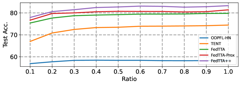
Figure 3. Each curve depicts the relationship between the size of test client datasets and the average test accuracy. In general, the larger the client dataset, the higher the test accuracy.

4.5. Concept Shift

Concept shift is also prevalent in federated learning, where the conditional distribution $p(x|y)$ varies among clients. We conduct additional experiments to demonstrate the effectiveness of FedTTA in the presence of concept shift during testing. Specifically, following FedSR (Nguyen et al., 2022), we create five domains with concept-shift among them: $M_{0}$, $M_{15}$, $M_{30}$, $M_{45}$, and $M_{60}$ by rotating the MNIST (LeCun et al., 1998) dataset counterclockwise at angles of [0, 15, 30, 45, 60] degrees. We set up 50 training clients with $M_{0}$, $M_{30}$, and $M_{60}$ while 50 test clients with $M_{15}$ and $M_{45}$. Please refer to the appendix for detailed statistics of the clients’ datasets.

We present the experiment results in Fig. 4. Significant concept shift makes it challenging to construct a well-perform ensemble model for test clients from the training clients. PFL-Sampled achieves a validation accuracy of 40.00 and a test accuracy of 9.92, while PFL-Ensemble achieves a validation accuracy of 67.06 and a test accuracy of 63.47. For better illustration, we exclude the results of PFL-Sampled and PFL-Ensemble from Fig. 4, as both methods exhibit very poor performance.

Fig. 4 clearly demonstrates the superior performance of our proposed methods. Specifically, on the test datasets, FedTTA  and FedTTA++  outperform the best baselines by 1.4% and 1.6%, respectively. Additionally, on the validation datasets, FedTTA  and FedTTA++  achieve results that are comparable to the best baselines.

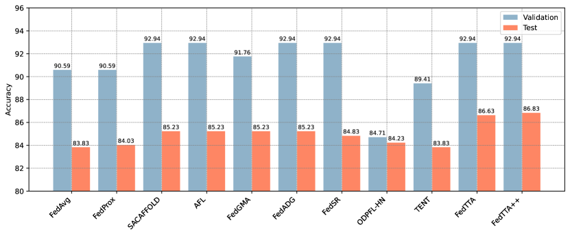
Figure 4. Performance comparison in the presence of concept shift. For better illustration, we exclude the results of PFL-Sampled and PFL-Ensemble here, as both methods exhibit very poor performance.

4.6. Heterogeneous Settings

In this subsection, we will investigate the effectiveness of our proposed KD loss function (Eq. 14) by running HeteroFedTTA on CIFAR-10 dataset with varying hyperparameter $\lambda\in\{0.0,0.2,0.4,0.6,\\ 0.8,1.0\}$. It is worth noting that when $\lambda$ equals zero, the loss degrades to the vanilla KD loss for FedTTA. For simplicity, we implement HeteroFedTTA  based on FedTTA  and use the same data partitioning as in the main experiment. We generate three types of models with different complexity levels by controlling the hidden channels, and we assign each model to a client with equal probability. $\eta_{inner}$, $\eta_{outer}$ and $\eta_{adapt}$ are set to 0.5, 0.1 and 0.005, respectively. For the detailed model structure, please refer to the appendix. TENT achieves the second best result after FedTTA  on CIFAR10 (see Table 1). We additionally implement heterogeneous TENT as a strong baseline by directly integrating TENT into the FedMD framework. We do not compare with ODPFL-HN in this experiment since the hypernetwork produces the same model structure for all clients.

Fig. 5 shows the test accuracy curves of TENT and HeteroFedTTA 
with different $\lambda$. The results indicate that HeteroFedTTA  is more effective and stable than TENT. Moreover, increasing the beta value generally improves the distillation effect. When $\lambda$ is approximately 0.8, it achieves the best performance, surpassing the vanilla KD by a significant margin. Overall, the experiment result validates the effectiveness of our proposed KD loss.

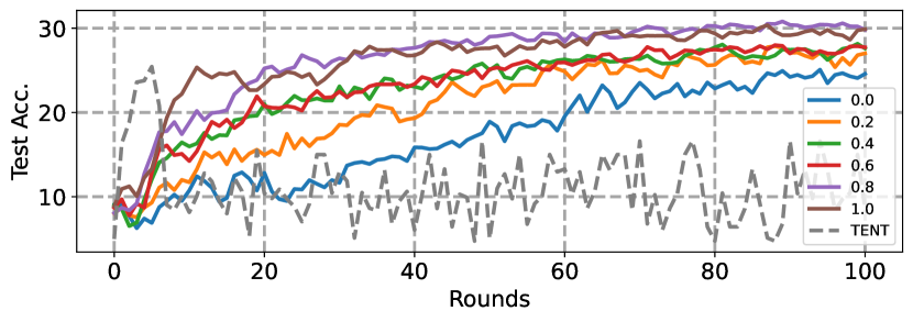
Figure 5. Test accuracy curves of TENT and HeteroFedTTA  with different $\lambda$ values.

5. Conclusion

In this paper, we investigated a practical yet challenging task for heterogeneous federated learning, i.e., Unsupervised Personalized Federated Learning towards new clients (UPFL), which aims to provide personalized models for unlabeled new clients after the federated model has been trained and deployed. To address the task, we first proposed a base method FedTTA, and we then improved FedTTA  with two simple yet effective optimization strategies: enhancing the adaptation model with regularization on the base prediction model and early-stopping the adaptation process through entropy. Last, we suggested a novel knowledge distillation loss for the special architecture of FedTTA and heterogeneous model setting. We conducted extensive experiments on five datasets and compare FedTTA and its variants against eleven baselines. The experimental results demonstrate the effectiveness of our proposed methods in addressing the UPFL task.

Appendix A Knowledge Distillation

We provide a schematic diagram of our proposed knowledge distillation loss in HeteroFedTTA in Fig.1. $\mathcal{D}_{p}$ is the public unlabeled dataset. $\{\psi^{s},\tilde{\psi}^{s}\}$ and $\{\psi^{t},\tilde{\psi}^{t}\}$ are the parameters of the base prediction model and the personalized prediction model of the student and the teacher, respectively, and $\phi^{s}$ is the parameters of the adaptation model of the student.

During the knowledge distillation process, the student should enforce its base prediction model and adaptation model learn from the corresponding models of the teacher, respectively. Specifically, $\psi^{s}$ should mimic the outputs of $\psi^{t}$, while $\phi^{s}$ should learn the personalization capability of $\phi^{t}$. Under the constraint of minimizing the KL-divergence between the outputs of $\psi^{s}$ and $\psi^{t}$, $\phi^{s}$ can learn the personalization ability of $\phi^{t}$ by minimizing the KL-divergence between the outputs of $\tilde{\psi}^{s}$ and $\tilde{\psi}^{t}$.

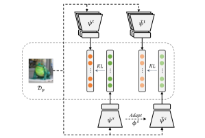
Figure 1. Schematic diagram of our proposed knowledge distillation loss in HeteroFedTTA. $\mathcal{D}_{p}$ is the public unlabeled dataset.

Appendix B Datasets

We first give a introduction to the datasets used, followed by details of the client partitions for all datasets. We conduct experiments on following five benchmark datasets, namely MNIST, CIFAR-10, FEMNIST, CIFAR-100 and Fashion-MNIST.

• MNIST: is a widely used handwritten digit recognition dataset, which consists of 10 classes of numerical digits 0-9.

• CIFAR-10: is a classic computer vision dataset that consists of 60,000 32x32 color images in 10 classes, where 50,000 images are used for training and the remaining 10,000 images are used for testing.

• FEMNIST: is a naturally heterogeneous dataset, which consists of 805,263 handwritten images from 3,550 users, where each user has a unique writing style.

• CIFAR-100: is a computer vision dataset that contains 60000 32x32 color images in 100 classes, where 50000 images are used for training and the remaining 10000 images are used for testing. The 100 classes in this dataset are grouped into 20 superclasses. Each image in the CIFAR-100 dataset is labeled with one of the 100 fine-grained classes and one of the 20 superclasses.

• Fashion-MNIST: is a 10-classes computer vision dataset, which consists of 70,000 28x28 grayscale images, each of which represents a fashion item.

For MNIST, CIFAR-10, CIFAR-100 and Fashion-MNIST, we union the training set and the test set, and then divide the entire data set into 100 clients in a non-IID manner. For MNIST, CIFAR-10 and Fahsion-MNIST, we partition the dataset by the pathological partition strategy, where each client contains at most two classes. For CIFAR-100, we divide the data of each superclass evenly to 5 clients, each client contains 5 classes out of 100 fine-grained classes. For FEMNIST, we sample 185 users from the 3,550 users for experiments. Then we randomly select 50% of the clients as training clients and the remaining 50% as test clients. For each training client, we partition the local dataset into train and validation splits with a ratio of 85:15. We present the details of the client partitions for all datasets in Tab. 1.

Table 1. Statistics of datasets used for experiments. FEMNIST is heterogeneous by nature, while the others follow pathological non-IID partitions.

Dataset	Classes	#Clients	#Samples	#Samples per client
MNIST	10	100	70,000	700
CIFAR-10	10	100	60,000	600
FEMNIST	62	185	40,272	218
CIFAR-100	100	100	60,000	600
Fashion-MNIST	10	100	70,000	700

Appendix C Baselines

We compare our proposed methods against following eleven baselines.

• FedAvg: is the first-proposed FL method, which proceeds between clients’ empirical risk minimization and server’s model aggregation.

• FedProx: is a reparameterization of FedAvg, which adds a proximal term to clients’ local objective functions to prevent significant divergence between the global model and local model.

• SCAFFOLD: leverages control variates to accelerate the model convergence.

• AFL: optimizes a centralized model for any possible target distribution formed by a mixture of the client distributions.

• FedGMA: proposes a gradient-masked averaging approach for federated learning that promotes the model to learn invariant mechanisms across clients.

• FedADG: employs the federated adversarial learning approach to measure and align the distributions among different source domains via matching each distribution to a adaptively generated reference distribution.

• FedSR: enforces an L2-norm regularizer on the representation and a conditional mutual information regularizer to encourage the model to only learn essential information.

• PFL-Sampled: selects a personalized model randomly from the training clients and sends it to the new client.

• PFL-Ensemble: sends all models from the training clients to the new client, and predictions are made by averaging the logits of all models.

• ODPFL-HN: simultaneously learns a client encoder network and a hyper-network, where the client encoder network takes the client’s unlabelled data as input and outputs the client representation, and the hyper-network generates personalized model weights based on the client’s representation.

• TENT: fine-tunes the model by minimizing the entropy of its predictions on the new client’s unlabelled data.

Table 2. Statistics of the clients’ datasets in the concept shift environment.

Clients	#Clients	Angles	#Total Samples	#Samples per client
Training	25	[0, 30, 60]	500	20
Testing	25	[15, 45]	500	20

Table 3. Three types of models with different complexity levels, i.e., small, medium and big.

Complexity	Prediction Model	Adaptation Model
Small	Conv(16)-Conv(32)-¿MLP(512)-¿MLP(10)	MLP(32)-¿MLP(32)-¿MLP(1)
Medium	Conv(32)-¿Conv(64)-¿MLP(512)-¿MLP(10)	MLP(64)-¿MLP(64)-¿MLP(1)
Big	Conv(64)-¿Conv(128)-¿MLP(512)-¿MLP(10)	MLP(128)-¿MLP(128)-¿MLP(1)

Appendix D Implementation Details

We provide a detailed implementation details of all methods. Particularly, we perform a grid search of hyperparameters for all methods, and the search space for each hyperparameter for each method is as follows:

• FedAvg: We search for the optimal learning rate of local optimization $\eta\in\{0.001,0.003,0.005,0.01,0.03,0.05,0.1,0.3,0.5\}$. It is important to note that unless explicitly mentioned, this search space for learning rates is applied to other methods as well.

• FedProx: We search for the optimal learning rate $\eta$ and coefficient of the proximal term $\mu\in\{0.001,0.01,0.1,1\}$.

• SCAFFOLD: We search for the optimal local learning rate $\eta_{l}$ and global learning rate $\eta_{g}$.

• AFL: We search for the optimal learning rates of model parameters $\gamma_{\omega}$ and mixture coefficient $\gamma_{\lambda}$.

• FedGMA: We search for the optimal learning rates of local learning rate $\eta_{l}$ and global learning rate $\eta_{g}$. The search space for $\eta_{g}$ is $\{0.01,0.1,1,1.5,2\}$. According to the paper (Tenison et al., 2022), we search for the optimal agreement threshold $\tau\in\{0.1,0.2,0.3,\\ 0.4,0.5,0.6,0.7,0.8,0.9\}$.

• FedADG: We set the dimension of the random noise to 10. The dimension of the learned feature representation is set to 128 for MNIST and 512 for other datasets. Additionally, we search for the optimal learning rate $\eta_{f}$ for the feature extractor and the classifier.

• FedSR: We search for the optimal learning rate $\eta$, and set the coefficients of the marginal distribution regularizer $\alpha^{L2R}$, and the conditional distribution regularizer $\alpha^{CMI}$ to their default values of 0.01 and 0.0005, respectively.

• PFL-Sampled and PFL-Ensemble: We search for the optimal learning rate $\eta$.

• ODPFL-HN: We search for the optimal learning rates for different components: the client encoder, denoted as $\eta_{encoder}$, the hyper-network, denoted as $\eta_{hn}$, and the local optimization, denoted as $\eta_{local}$. The client embedding size is set to 32 across all datasets.

• TENT: We apply the searched optimal learning rates from FedAvg to TENT.

• FedTTA: We fine-tune the inner learning rate of the prediction model, denoted as $\eta_{inner}$, the outer learning rate of the prediction model, denoted as $\eta_{outer}$, and the learning rate of the adaptation model, denoted as $\eta_{adapt}$.

• FedTTA++: In addition to searching for the optimal values of $\eta_{inner}$, $\eta_{outer}$ and $\eta_{adapt}$, we also search for the optimal coefficient of the proximal term $\mu\in\{0.001,0.01,0.1,1\}$. In FedTTA++, we propose to stop the adaptation process when the entropy of the personalized prediction model’s predictions does not decrease within a certain patience value. We search for the best value of the patience from $\{1,3,5\}$.

We present the searched optimal hyperparameters in Tab.4.

Table 4. Hyper-parameter setting details of our proposed methods and the baselines on all datasets.

Method	MNIST	CIFAR-10	FEMNIST	CIFAR-100	Fashion-MNIST
FedAvg	$\eta=0.1$	$\eta=0.1$	$\eta=0.1$	$\eta=0.1$	$\eta=0.3$
FedProx	$\eta=0.3,\mu=0.001$	$\eta=0.1,\mu=0.001$	$\eta=0.3,\mu=0.001$	$\eta=0.1,\mu=0.001$	$\eta=0.3,\mu=0.001$
SCAFFOLD	$\eta_{l}=0.1,\eta_{g}=1.5$	$\eta_{l}=0.1,\eta_{g}=1.5$	$\eta_{l}=0.1,\eta_{g}=1.5$	$\eta_{l}=0.1,\eta_{g}=1.5$	$\eta_{l}=0.1,\eta_{g}=1.5$
AFL	$\gamma_{\omega}=0.3,\gamma_{\lambda}=0.001$	$\gamma_{\omega}=0.1,\gamma_{\lambda}=0.3$	$\gamma_{\omega}=0.1,\gamma_{\lambda}=0.5$	$\gamma_{\omega}=0.1,\gamma_{\lambda}=0.3$	$\gamma_{\omega}=0.3,\gamma_{\lambda}=0.001$
FedGMA	$\eta_{c}=0.3,\eta_{g}=1,\tau=0.1$	$\eta_{c}=0.1,\eta_{g}=1.5,\tau=0.1$	$\eta_{c}=0.3,\eta_{g}=1,\tau=0.1$	$\eta_{c}=0.1,\eta_{g}=1.5,\tau=0.1$	$\eta_{c}=0.3,\eta_{g}=1.5,\tau=0.1$
FedADG	$\eta_{f}=0.3$	$\eta_{f}=0.1$	$\eta_{f}=0.3$	$\eta_{f}=0.1$	$\eta_{f}=0.3$
FedSR	$\eta=0.3$	$\eta=0.05$	$\eta=0.3$	$\eta=0.1$	$\eta=0.3$
PFL-Sampled	$\eta=0.1$	$\eta=0.1$	$\eta=0.1$	$\eta=0.1$	$\eta=0.3$
PFL-Ensemble	$\eta=0.1$	$\eta=0.1$	$\eta=0.1$	$\eta=0.1$	$\eta=0.3$
ODPFL-HN	$\eta_{local}=0.3,\eta_{encoder}=0.5,\eta_{hn}=0.5$	$\eta_{local}=0.05,\eta_{encoder}=0.1,\eta_{hn}=0.5$	$\eta_{local}=0.01,\eta_{encoder}=0.1,\eta_{hn}=0.5$	xx	$\eta_{local}=0.1,\eta_{encoder}=0.5,\eta_{hnet}=0.5$
TENT	$\eta=0.1$	$\eta=0.1$	$\eta=0.1$	$\eta=0.1$	$\eta=0.3$
FedTTA	$\eta_{inner}=0.5,\eta_{outer}=0.3,\eta_{adapt}=0.01$	$\eta_{inner}=0.5,\eta_{outer}=0.05,\eta_{adapt}=0.005$	$\eta_{inner}=0.3,\eta_{outer}=0.1,\eta_{adapt}=0.003$	$\eta_{inner}=0.5,\eta_{outer}=0.1,\eta_{adapt}=0.001$	$\eta_{inner}=0.05,\eta_{outer}=0.1,\eta_{adapt}=0.001$
FedTTA-Prox	$\eta_{inner}=0.5,\eta_{outer}=0.3,\eta_{adapt}=0.001,\mu=0.01$	$\eta_{inner}=0.3,\eta_{outer}=0.1,\eta_{adapt}=0.003,\mu=0.001$	$\eta_{inner}=0.3,\eta_{outer}=0.1,\eta_{adapt}=0.003,\mu=0.001$	$\eta_{inner}=0.5,\eta_{outer}=0.1,\eta_{adapt}=0.001,\mu=0.01$	$\eta_{inner}=0.05,\eta_{outer}=0.1,\eta_{adapt}=0.001,\mu=0.001$
FedTTA++	$patience=1$	$patience=1$	$patience=5$	$patience=5$	$patience=5$

Appendix E Learning Efficiency

We present the accuracy curves of all methods on all datasets in Fig. 2. Compared with FedAvg, FedProx, and the GFL methods, SCAFFOLD generally converges faster and achieves higher accuracy. Due to distribution shift between training clients and test clients, TENT shows inconsistent convergence behavior on the validation set and the test set for CIFAR-10 and CIFAR-100, resulting in inconsistent best models on the validation and test sets. FedTTA and FedTTA-Prox exhibit similar convergence behavior. FedTTA++ quickly converges to the best result but is somewhat unstable in the first several communication rounds. We attribute this to the global base prediction model and adaptation model being undertrained and entropy minimization leading to overconfidence towards incorrect predictions. Additionally, FedTTA  and its variants behave similarly on the validation and test sets.

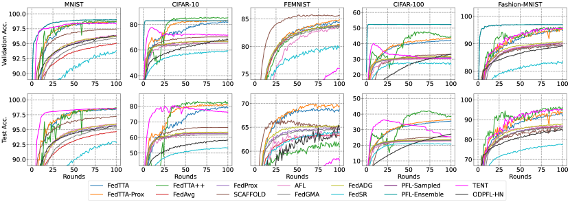
Figure 2. Convergence comparison of FedTTA and its variants with the baselines. Each learning curve is averaged over three random seeds.

Appendix F Concept Shift

We randomly sample 1,000 instances from the union of the training set and test set of MNIST and allocate these samples to 50 clients in an IID (independent and identically distributed) manner. Among these clients, 25 are selected as training clients, and the remaining 25 are designated as testing clients. For the training clients, each client applies a fixed rotation angle to its local dataset, randomly selected from the set of [0, 30, 60] degrees with equal probability. On the other hand, the testing clients rotate their respective local datasets at a fixed angle, randomly selected from the set of [15, 45] degrees with equal probability. We present the partitioning information of the clients in Tab. 2.

Appendix G Heterogeneous Models

We generate three types of models with different complexity levels (small, medium and big) by controlling the hidden channels, and we assign each model to a client with equal probability. We present the detailed model structure of each complexity level in Tab. 3.

References

- (1)
- Amosy et al. (2021) Ohad Amosy, Gal Eyal, and Gal Chechik. 2021. On-Demand Unlabeled Personalized Federated Learning. arXiv preprint arXiv:2111.08356 (2021).
- Arivazhagan et al. (2019) Manoj Ghuhan Arivazhagan, Vinay Aggarwal, Aaditya Kumar Singh, and Sunav Choudhary. 2019. Federated learning with personalization layers. arXiv preprint arXiv:1912.00818 (2019).
- Caldarola et al. (2022) Debora Caldarola, Barbara Caputo, and Marco Ciccone. 2022. Improving generalization in federated learning by seeking flat minima. In Computer Vision–ECCV 2022: 17th European Conference, Tel Aviv, Israel, October 23–27, 2022, Proceedings, Part XXIII. Springer, 654–672.
- Caldas et al. (2018) Sebastian Caldas, Sai Meher Karthik Duddu, Peter Wu, Tian Li, Jakub Konečnỳ, H Brendan McMahan, Virginia Smith, and Ameet Talwalkar. 2018. Leaf: A benchmark for federated settings. arXiv preprint arXiv:1812.01097 (2018).
- Fallah et al. (2020) Alireza Fallah, Aryan Mokhtari, and Asuman Ozdaglar. 2020. Personalized federated learning with theoretical guarantees: A model-agnostic meta-learning approach. Advances in Neural Information Processing Systems 33 (2020), 3557–3568.
- Gao et al. (2022) Dashan Gao, Xin Yao, and Qiang Yang. 2022. A Survey on Heterogeneous Federated Learning. arXiv preprint arXiv:2210.04505 (2022).
- Goodfellow et al. (2014) Ian J. Goodfellow, Jean Pouget-Abadie, Mehdi Mirza, Bing Xu, David Warde-Farley, Sherjil Ozair, Aaron C. Courville, and Yoshua Bengio. 2014. Generative Adversarial Nets. In NIPS.
- Hsu et al. (2019) Tzu-Ming Harry Hsu, Hang Qi, and Matthew Brown. 2019. Measuring the Effects of Non-Identical Data Distribution for Federated Visual Classification. arXiv:1909.06335 [cs.LG]
- Jiang and Lin (2022) Liangze Jiang and Tao Lin. 2022. Test-Time Robust Personalization for Federated Learning. arXiv preprint arXiv:2205.10920 (2022).
- Kairouz et al. (2021) Peter Kairouz, H Brendan McMahan, Brendan Avent, Aurélien Bellet, Mehdi Bennis, Arjun Nitin Bhagoji, Kallista Bonawitz, Zachary Charles, Graham Cormode, Rachel Cummings, et al. 2021. Advances and open problems in federated learning. Foundations and Trends® in Machine Learning 14, 1–2 (2021), 1–210.
- Karimireddy et al. (2020) Sai Praneeth Karimireddy, Satyen Kale, Mehryar Mohri, Sashank Reddi, Sebastian Stich, and Ananda Theertha Suresh. 2020. Scaffold: Stochastic controlled averaging for federated learning. In International Conference on Machine Learning. PMLR, 5132–5143.
- Krizhevsky (2009) Alex Krizhevsky. 2009. CIFAR-10 Dataset. http://www.cs.toronto.edu/~kriz/cifar.html.
- Krizhevsky et al. (2009) Alex Krizhevsky, Vinod Nair, and Geoffrey Hinton. 2009. CIFAR-100 Dataset. http://www.cs.toronto.edu/~kriz/cifar.html.
- LeCun et al. (1998) Yann LeCun, Léon Bottou, Yoshua Bengio, and Patrick Haffner. 1998. Gradient-based learning applied to document recognition. Proc. IEEE 86, 11 (1998), 2278–2324.
- Li and Wang (2019) Daliang Li and Junpu Wang. 2019. Fedmd: Heterogenous federated learning via model distillation. arXiv preprint arXiv:1910.03581 (2019).
- Li et al. (2020) Tian Li, Anit Kumar Sahu, Manzil Zaheer, Maziar Sanjabi, Ameet Talwalkar, and Virginia Smith. 2020. Federated optimization in heterogeneous networks. Proceedings of Machine learning and systems 2 (2020), 429–450.
- Liu et al. (2021a) Quande Liu, Cheng Chen, Jing Qin, Qi Dou, and Pheng-Ann Heng. 2021a. Feddg: Federated domain generalization on medical image segmentation via episodic learning in continuous frequency space. In Proceedings of the IEEE/CVF Conference on Computer Vision and Pattern Recognition. 1013–1023.
- Liu et al. (2021b) Yuejiang Liu, Parth Kothari, Bastien Van Delft, Baptiste Bellot-Gurlet, Taylor Mordan, and Alexandre Alahi. 2021b. TTT++: When does self-supervised test-time training fail or thrive? Advances in Neural Information Processing Systems 34 (2021), 21808–21820.
- McMahan et al. (2017) Brendan McMahan, Eider Moore, Daniel Ramage, Seth Hampson, and Blaise Aguera y Arcas. 2017. Communication-efficient learning of deep networks from decentralized data. In Artificial intelligence and statistics. PMLR, 1273–1282.
- Mohri et al. (2019) Mehryar Mohri, Gary Sivek, and Ananda Theertha Suresh. 2019. Agnostic federated learning. In International Conference on Machine Learning. PMLR, 4615–4625.
- Nguyen et al. (2022) A Tuan Nguyen, Philip Torr, and Ser-Nam Lim. 2022. FedSR: A Simple and Effective Domain Generalization Method for Federated Learning. In Advances in Neural Information Processing Systems.
- Qu et al. (2022) Zhe Qu, Xingyu Li, Rui Duan, Yao Liu, Bo Tang, and Zhuo Lu. 2022. Generalized federated learning via sharpness aware minimization. In International Conference on Machine Learning. PMLR, 18250–18280.
- Shamsian et al. (2021) Aviv Shamsian, Aviv Navon, Ethan Fetaya, and Gal Chechik. 2021. Personalized federated learning using hypernetworks. In International Conference on Machine Learning. PMLR, 9489–9502.
- Sun et al. (2020) Yu Sun, Xiaolong Wang, Zhuang Liu, John Miller, Alexei Efros, and Moritz Hardt. 2020. Test-time training with self-supervision for generalization under distribution shifts. In International conference on machine learning. PMLR, 9229–9248.
- Tenison et al. (2022) Irene Tenison, Sai Aravind Sreeramadas, Vaikkunth Mugunthan, Edouard Oyallon, Eugene Belilovsky, and Irina Rish. 2022. Gradient masked averaging for federated learning. arXiv preprint arXiv:2201.11986 (2022).
- Wang et al. (2020) Dequan Wang, Evan Shelhamer, Shaoteng Liu, Bruno Olshausen, and Trevor Darrell. 2020. Tent: Fully test-time adaptation by entropy minimization. arXiv preprint arXiv:2006.10726 (2020).
- Xiao et al. (2017) Han Xiao, Kashif Rasul, and Roland Vollgraf. 2017. Fashion-mnist: a novel image dataset for benchmarking machine learning algorithms. arXiv preprint arXiv:1708.07747 (2017).
- Zhang et al. (2021a) Jie Zhang, Song Guo, Xiaosong Ma, Haozhao Wang, Wenchao Xu, and Feijie Wu. 2021a. Parameterized knowledge transfer for personalized federated learning. Advances in Neural Information Processing Systems 34 (2021), 10092–10104.
- Zhang et al. (2021b) Liling Zhang, Xinyu Lei, Yichun Shi, Hongyu Huang, and Chao Chen. 2021b. Federated learning with domain generalization. arXiv preprint arXiv:2111.10487 (2021).
- Zhang et al. (2021c) Marvin Zhang, Henrik Marklund, Nikita Dhawan, Abhishek Gupta, Sergey Levine, and Chelsea Finn. 2021c. Adaptive risk minimization: Learning to adapt to domain shift. Advances in Neural Information Processing Systems 34 (2021), 23664–23678.
- Zhu et al. (2021) Zhuangdi Zhu, Junyuan Hong, and Jiayu Zhou. 2021. Data-free knowledge distillation for heterogeneous federated learning. In International Conference on Machine Learning. PMLR, 12878–12889.