Quantum Electrodynamic Corrections to Cyclotron States in a Penning Trap

Abstract

We analyze the leading and higher-order quantum electrodynamic corrections to the energy levels for a single electron bound in a Penning trap, including the Bethe logarithm correction due to virtual excitations of the reference quantum cyclotron state. The effective coupling parameter $\alpha_{c}$ in the Penning trap is identified as the square root of the ratio of the cyclotron frequency, converted to an energy via multiplication by the Planck constant, to the electron rest mass energy. We find a large, state-independent, logarithmic one-loop self-energy correction of order $\alpha\,\alpha_{c}^{4}\,mc^{2}\ln(\alpha_{c}^{-2})$, where $m$ is the electron rest mass and $c$ is the speed of light. Furthermore, we find a state-independent “trapped” Bethe logarithm. We also obtain a state-dependent higher-order logarithmic self-energy correction of order $\alpha\,\alpha_{c}^{6}\,mc^{2}\,\ln(\alpha_{c}^{-2})$. In the high-energy part of the bound-state self energy, we need to consider terms with up to six magnetic interaction vertices inside the virtual photon loop.

I Introduction

Relativistic and quantum electrodynamic corrections to the quantum cyclotron energy levels in a Penning trap are of essential importance for the determination of fundamental physical constants Brown and Gabrielse (1982); Brown et al. (1985); Brown and Gabrielse (1986); GaE ; Hanneke et al. (2008); Fan et al. (2023). In a recent article Wienczek et al. (2022), higher-order relativistic corrections for the energy levels in a quantum cyclotron have been analyzed. Here, our goal is to supplement the preceding analysis Wienczek et al. (2022) by a calculation of the intricate and notoriously problematic quantum electrodynamic (QED) corrections to the quantum cyclotron energy levels inside the Penning trap. In our calculations, we use expansion parameters which allow us to initiate a systematic classification of the correction terms, in terms of a semi-analytic expansion in terms of a “trapped fine-structure constant $\alpha_{c}$”, and a cyclotron scaling parameter $\xi_{c}$, as well as an axial scaling parameter $\xi_{z}$. These parameters replace and supplement the QED coupling parameter, which is the fine-structure constant $\alpha$.

As already anticipated, the effective coupling parameter in a quantum cyclotron could be identified as the maximum of the cyclotron ($c$) and the axial ($z$) coupling constants. In particular, one may identify the coupling parameters (in a unit system with $\hbar=c=\epsilon_{0}=1$)

$$\alpha_{c}=\sqrt{\frac{\omega_{c}}{m}}\,,\qquad\alpha_{z}=\sqrt{\frac{\omega_{z}}{m}}\,,\qquad\omega_{c}=\frac{|e|\,B_{\rm T}}{m}\,,$$ (1)

which depend on the cyclotron frequency $\omega_{c}$, and the axial frequency $\omega_{z}$. The cyclotron frequency Brown and Gabrielse (1986) is $\omega_{c}=|e|\,B_{\mathrm{T}}/m$, where $e$ is the electron charge, $|e|=-e$ is the (positive) elementary charge, $B_{\mathrm{T}}$ is the magnetic field in the Penning trap, and $m$ is the electron mass.

The hierarchy of typical frequencies in a Penning trap Brown and Gabrielse (1986); Wienczek et al. (2022) implies that the magnetron frequency $\omega_{\mathrm{m}}$ is much smaller than the axial frequency $\omega_{z}$. Following the conventions of Ref. Brown and Gabrielse (1986), we define the corrected cyclotron frequency as $\omega_{\mbox{\scriptsize$(+)$}}$, we define the corrected magnetron frequency as $\omega_{\mathrm{m}}=\omega_{\mbox{\scriptsize$(-)$}}$, where

$$\omega_{\mbox{\scriptsize$(+)$}}= \;\frac{1}{2}\,\left(\omega_{c}+\sqrt{\omega_{c}^{2}-2\omega_{z}^{2}}\right)\,,$$ (2a)

$$\omega_{\mbox{\scriptsize$(-)$}}= \;\omega_{\mathrm{m}}=\frac{1}{2}\,\left(\omega_{c}-\sqrt{\omega_{c}^{2}-2\omega_{z}^{2}}\right)\approx\frac{\omega_{z}^{2}}{2\omega_{c}}\,.$$ (2b)

The magnetron frequency is, typically, much smaller than the cyclotron frequency $\omega_{c}$. One defines the generalized coupling parameter

$$\alpha_{\mathrm{m}}=\sqrt{\frac{\omega_{\mathrm{m}}}{m}}$$ (3)

for the magnetron frequency. We assume the following hierarchy to be fulfilled (see Ref. Brown and Gabrielse (1986)),

$$\alpha_{\mathrm{m}}\ll\alpha_{z}\ll\alpha_{c}\,.$$ (4)

We also define scaling parameters $\xi_{z}$ and $\xi_{\mathrm{m}}$ by

$$\alpha_{z}= \;\xi_{z}\,\alpha_{c}\,,\qquad\alpha_{\mathrm{m}}=\xi_{\mathrm{m}}\,\alpha_{c}\,,$$ (5)

$$\xi_{\mathrm{m}}= \;\frac{1}{\sqrt{2}}\left(1-\sqrt{1-2\xi_{z}^{4}}\right)^{1/2}\approx\frac{\xi_{z}^{2}}{\sqrt{2}}\,.$$ (6)

The hierarchy of the frequencies allows us to perform a systematic expansion in terms of $\alpha_{c}$, $\xi_{z}$ and $\xi_{\mathrm{m}}$, as well as the coupling parameter of quantum electrodynamics, that is, the fine-structure constant $\alpha$. The expansion in $\xi_{\mathrm{m}}$ gives rise to an expansion in $\xi_{z}^{2}$, and we can henceforth use the parameter $\xi_{z}$ in order to universally describe the parametrically suppressed effects due to both the axial as well as magnetron motions.

A remark is in order, concerning the anticipated results of our studies. It is well known Bethe (1947); Pachucki (1993); Jentschura and Pachucki (1996) that the leading logarithmic quantum electrodynamic self-energy correction to hydrogen energy levels is proportional to (in natural units, $\hbar=c=\epsilon_{0}=1$, which are used here)

$$\Delta E_{\rm QED}\sim\alpha\,(Z\alpha)^{4}\,m\,\ln[(Z\alpha)^{-2}]\,,$$ (7)

where $\alpha$ is the fine-structure constant, and $Z$ is the nuclear charge number. We here anticipate that we shall find the following, analogous scaling for the leading quantum electrodynamic self-energy correction to quantum cyclotron levels in a Penning trap,

$$\Delta E_{\rm QED}\sim\alpha\,\alpha_{c}^{4}\,m\,\ln(\alpha_{c}^{-2})\,,$$ (8)

where the coefficient $\alpha$ is due to the absorption and emission of the virtual photon, and the factors of $\alpha_{c}$ describe the binding to the trap fields, which is typically smaller than the coupling parameter $\alpha$ for atoms. It is our goal to calculate these energy shifts.

This paper is organized as follows. In Sec. II, we present a brief review of the quantum cyclotron states which enter our formalism. Vacuum-polarization corrections are negligible for quantum cyclotron states, for reasons outlined in Sec. III. Self-energy effects are discussed in Sec. IV; these constitute the dominant radiative corrections for quantum cyclotron states. Conclusions are reserved for Sec. V.

II Quantum Cyclotron Levels

In order to understand the quantum cyclotron levels inside a Penning trap, it is, first of all, necessary to remember that the kinetic momentum is given by

$$\vec{\pi}_{\mathrm{T}}=\vec{p}-e\vec{A}_{\mathrm{T}}=\vec{p}-\frac{e}{2}\,(\vec{B}_{\mathrm{T}}\times\vec{r})\,,$$ (9)

where $\vec{A}_{\mathrm{T}}=\tfrac{1}{2}(\vec{B}_{\mathrm{T}}\times\vec{r})$ is the vector potential, $\vec{B}_{\mathrm{T}}=B_{\mathrm{T}}\,\hat{\mathrm{e}}_{z}$ is the magnetic field in the trap, and $\vec{p}=-\mathrm{i}\vec{\nabla}$ is the kinetic momentum operator. The kinetic momentum $\vec{\pi}_{\mathrm{T}}$ enters the interaction Hamiltonian describing the coupling of the bound electron (inside the Penning trap) to the quantized electromagnetic field.

The quadrupole electric field in the trap is attractive along the $z$ axis and repulsive in the $xy$ plane,

$$V= \;=V_{z}+V_{\parallel}\,,\qquad\vec{\nabla}^{2}V=0\,,$$ (10a)

$$V_{z}= \;\frac{1}{2}m\omega_{z}^{2}z^{2}\qquad V_{\parallel}=-\frac{1}{4}m\omega_{z}^{2}\rho^{2}\,.$$ (10b)

The unperturbed Hamiltonian is given as follows,

$$H_{0}=\frac{(\vec{\sigma}\cdot\vec{\pi}_{\mathrm{T}})^{2}}{2m}+V-\frac{e}{2m}\,\kappa\,\vec{\sigma}\cdot\vec{B}_{\mathrm{T}}\,.$$ (11)

Eigenstates of the unperturbed Hamiltonian $H_{0}$ are described Brown and Gabrielse (1986) by four quantum numbers: the axial quantum number $k$, the magnetron quantum number $\ell$, the cyclotron quantum number $n$, and the spin projection quantum number $s=\pm 1$. These take on the following values: $k=0,1,2,\dots$ (axial), $\ell=0,1,2,\dots$ (magnetron), $n=0,1,2,\dots$ (cyclotron), and $s=\pm 1$ (spin). We recall, from Ref. Wienczek et al. (2022), the energy eigenvalues of $H_{0}$,

$$E_{k\ell ns}= \;\omega_{c}(1+\kappa)\,\frac{s}{2}+\omega_{\mbox{\scriptsize$(+)$}}\left(n+\frac{1}{2}\right)$$

$$\;+\omega_{z}\left(k+\frac{1}{2}\right)-\omega_{\mbox{\scriptsize$(-)$}}\left(\ell+\frac{1}{2}\right)\,.$$ (12)

It is of note that, in view of the repulsive character of the quadrupole potential, these eigenvalues are not bounded from below. We use the conventions of Refs. Brown and Gabrielse (1986); Wienczek et al. (2022), for the cyclotron lowering and raising operators $a_{\mbox{\scriptsize$(+)$}}$ and $a^{\dagger}_{\mbox{\scriptsize$(+)$}}$, the axial lowering and raising operators $a_{z}$ and $a^{\dagger}_{z}$, and the magnetron lowering and raising operators $a_{\mbox{\scriptsize$(-)$}}$ and $a^{\dagger}_{\mbox{\scriptsize$(-)$}}$. The eigenstates of the unperturbed Hamiltonian are given as follows,

$$\psi_{k\ell ns}(\vec{r})= \;\frac{\left(a^{\dagger}_{\mbox{\scriptsize$(+)$}}\right)^{n}}{\sqrt{n!}}\,\frac{\left(a^{\dagger}_{z}\right)^{k}}{\sqrt{k!}}\,\frac{\left(a^{\dagger}_{\mbox{\scriptsize$(-)$}}\right)^{q}}{\sqrt{q!}}\,\psi_{0}(\vec{r})\,\chi_{s/2}\,,$$

$$\chi_{1/2}= \;\left(\begin{array}[]{c}1\\ 0\end{array}\right)\,,\qquad\chi_{-1/2}=\left(\begin{array}[]{c}0\\ 1\end{array}\right)\,.$$ (17)

The orbital part of the ground-state wave function is

$$\psi_{0}(\vec{r})= \;\sqrt{\frac{m\sqrt{\omega_{c}^{2}-2\omega_{z}^{2}}}{2\pi}}\,\exp\left(-\frac{m}{4}\sqrt{\omega_{c}^{2}-2\omega_{z}^{2}}\,\rho^{2}\right)$$

$$\;\times\left(\frac{m\omega_{z}}{\pi}\right)^{1/4}\,\exp\left(-\frac{1}{2}m\omega_{z}z^{2}\right)\,.$$ (18)

The spin-up sublevel of the $n$th cyclotron ground state, and the spin-down sublevel of the $(n+1)$st excited cyclotron state, are quasi-degenerate and of interest for spectroscopy and determination of the anomalous magnetic moment of the electron Brown and Gabrielse (1982); Brown et al. (1985); GaE ; Hanneke et al. (2008); Fan et al. (2023).

III Vacuum Polarization

For atomic bound states, quantum electrodynamic energy shifts are naturally separated into vacuum-polarization and self-energy corrections. The vacuum-polarization shift of a hydrogenic energy level is due to the screening of the proton’s charge by virtual electron-positron pairs. The closer the electron is to the nucleus, the less pronounced is the screening of the bare proton charge, and the stronger is the (corrected) Coulomb potential. The dominant contribution to the one-loop effect is described by the Uehling potential Uehling (1935). In a Penning trap, the potential is generated by the trap electrodes in addition to the axial magnetic field. Hence, the electron, on its quantum cyclotron orbit, is always sufficiently far away from any other charged particle that the vacuum-polarization energy shift can be safely neglected. This statement can be quantified as follows.

The long-range tail of the Uehling potential is given as follows Jentschura (2011a),

$$V_{U}(r)\approx-\frac{\alpha(Z\alpha)m}{4\sqrt{\pi}}\,\frac{\exp(-mr)}{(m\,r)^{5/2}}\,,\qquad r\to\infty\,,$$ (19)

where $r$ is the distance from the nucleus. The one-loop Uehling correction needs to be compared to the Coulomb potential,

$$V_{C}(r)\approx-\frac{Z\alpha m}{(mr)}\,,$$ (20)

leading to the relative correction,

$$\frac{V_{U}(r)}{V_{C}(r)}\approx\frac{\alpha}{4\sqrt{\pi}\,(mr)^{3/2}}\,\exp(-mr)\,,\qquad r\to\infty\,,$$ (21)

A typical Penning trap dimension Brown and Gabrielse (1986) is of the order of about $\langle r\rangle\sim 1\,{\rm cm}$, while the quantity $m\,r$ is dimensionless in natural units. When converted to Système International (mksA) units, one realizes that $m$ takes the role of the inverse of the reduced Compton wavelength of the electron,

$$mr=\frac{r}{\lambdabar_{e}}=2.59\times 10^{12}\,\times R\,,\qquad R=\frac{r}{1\,{\rm m}}\,,$$ (22)

where $R$ is measured in meters. For $R$ being on the order of $1\,{\rm cm}$, one has $mr$ on the order of $10^{10}$. The quantity

$$\exp(-m\langle r\rangle)\sim\exp(-10^{10})\approx 10^{-4.3\times 10^{9}}$$ (23)

is very small indeed. Its smallness illustrates that, because of the exponential expression of the one-loop vacuum-polarization correction to the quadrupole trap potential, the vacuum-polarization corrections can be neglected. The same exponential suppression factor $\exp(-mr)$ enters the magnetic photon exchange Jentschura (2011b) which is the basis for the magnetic field of the trap. Therefore, vacuum-polarization corrections can be safely neglected for quantum cyclotron levels.

IV Self Energy

IV.1 Orientation

Inspired by the formalism pertinent to bound states in a Coulomb field Jentschura and Pachucki (1996); Jentschura et al. (1997), we write the semi-analytic expansion of the one-loop bound-state energy shift of a quantum cyclotron state as follows,

$$E_{\rm SE}=\frac{\alpha}{\pi}\,m\sum_{rs}\mathcal{A}_{rs}\,(\alpha_{c})^{r}\,\ln^{s}\left(\alpha_{c}^{-2}\right)$$ (24)

where the first subscript of the $\mathcal{A}$ coefficients counts the power of $\alpha_{c}$, and the second subscript indicates the power of the logarithm $\ln\left(\alpha_{c}^{-2}\right)$.

The $\mathcal{A}_{rs}$ coefficients are analogous to the coefficients $A_{rs}$ used in Lamb shift calculations for hydrogenlike systems (see Sec. 15.4 of Ref. Jentschura and Adkins (2022)). For the electron in the Penning trap, the role of the Coulombic coupling parameter $Z\alpha$ is taken by the cyclotron coupling parameter $\alpha_{c}$. In Lamb shift calculations for hydrogenic systems, one scales out a factor $1/n^{3}$ from the coefficients, where $n$ is the principal quantum number. This reflects on the typical scaling of quantum electrodynamic energy corrections in hydrogenlike systems. In the Penning trap, the role of $n$ is played by the cyclotron quantum number. However, there is a decisive difference: For the Penning trap, no $1/n^{3}$ dependence is incurred, and in fact, some logarithmic coefficients are seen to increase with $n$, not decrease as is typically the case in Coulombic bound systems. We thus do not scale out $1/n^{3}$ in the definition of the $\mathcal{A}_{rs}$ coefficients.

The leading self-energy coefficient is seen to be $\mathcal{A}_{20}$, and is due to the leading Schwinger term Schwinger (1948) in the anomalous magnetic moment of the electron. Here, we focus on the coefficients $\mathcal{A}_{20}$, $\mathcal{A}_{41}$, $\mathcal{A}_{40}$, and $\mathcal{A}_{61}$, which constitute the leading nonvanishing coefficients for a general quantum cyclotron state. The higher-order nonlogarithmic coefficients possess an expansion in powers of $\xi_{z}$, e.g., $\mathcal{A}_{40}=\left.\mathcal{A}_{40}\right|_{\xi_{z}=0}+\mathcal{O}(\xi_{z})$. We here evaluate $\mathcal{A}_{20}$, $\mathcal{A}_{41}$ and $\mathcal{A}_{61}$, and $\mathcal{A}_{40}$ in the leading order in $\xi_{z}$, and partial results for the corrections proportional to $\xi_{\mathrm{m}}$ and $\xi_{z}$. The Bethe logarithm inside the Penning trap is seen to contribute to $\mathcal{A}_{40}$, albeit only at order $\xi_{z}$. Indeed, in the leading order in the expansion in $\xi_{z}$, the Bethe logarithm in the Penning trap will be seen to vanish. Our result for the Bethe logarithm is numerically small and, somewhat surprisingly, state-independent. The contribution of the Bethe logarithm is thus not visible in any transitions among quantum cyclotron states. Let us anticipate some results which will be derived in the following, in order to lay out the work program of our article. Indeed, we obtain two contributions to the order-$\xi_{z}$ correction to $\mathcal{A}_{40}$, one from a higher-order anomalous magnetic moment term, and a second one from the Bethe logarithm. There might be another contribution to the order-$\xi_{z}$ correction to $\mathcal{A}_{40}$, from the high-energy part, which we evaluate only to leading order in $\xi_{z}$. The evaluation of the complete order-$\xi_{z}$ correction to $\mathcal{A}_{40}$ will be left for a future investigation. The dominant state-dependent correction, in the leading order in $\xi_{\mathrm{m}}$ and $\xi_{z}$, is found to be given by the $\mathcal{A}_{61}$ coefficient.

The coefficients $\mathcal{A}_{20}$, $\mathcal{A}_{41}$, $\mathcal{A}_{40}$, and $\mathcal{A}_{61}$, determined here, constitute the leading nonvanishing coefficients for the self-energy effect. Coefficients of odd order in $\alpha_{c}$ such as $\mathcal{A}_{31}$ and $\mathcal{A}_{30}$, as well as $\mathcal{A}_{50}$, vanish. [By odd order, in general, we refer to an odd integer $r$ in Eq. (24).] A brief discussion on this point, mostly based on the high-energy part discussed in Sec. IV.3, is in order. The $\mathcal{A}_{20}$ coefficients is a consequence of the Schwinger term Schwinger (1948) which enters at lower order because the main binding potential involves the magnetic trap field. Operators in the high-energy part can be expanded in the (vector-)potential $\Gamma_{\mathrm{T}}$ defined in Eq. (45) and in the momentum operators. For quantum cyclotron states, momentum and potential operators (coordinates) can be expressed in terms of raising and lowering operators of the cyclotron and magnetron quantum numbers Wienczek et al. (2022), and hence, all of these matrix elements are convergent (in arbitrarily high orders in $\alpha_{c}$). Because of symmetry reasons, matrix elements which would otherwise lead to an odd power of $\alpha_{c}$ vanish. An example would be terms of third order in the momentum operators, whose matrix element on the reference state vanishes due to parity. [Odd orders in $\alpha_{c}$ would otherwise correspond to half-integer powers in $\omega_{c}$, in view of Eq. (1).]

The terms $\mathcal{A}_{41}$ and $\mathcal{A}_{40}$ are generated by mechanism much in analogy to those at work in Coulombic bound systems (see Chaps. 4 and 11 of Ref. Jentschura and Adkins (2022)). Finally, one might ask why the term $\mathcal{A}_{50}$ vanishes for quantum cyclotron levels in a Penning trap, while the corresponding term $A_{50}$ for Coulombic systems is nonvanishing (see Chap. 15 of Ref. Jentschura and Adkins (2022) and Ref. Baranger et al. (1953)). A closer inspection reveals that the emergence of the $A_{50}$ term (for radially symmetric $S$ states in Coulombic systems) is caused by the singularity of the Coulomb potential and of the hydrogen eigenstates. The singularity of the Coulomb potential eventually leads to the divergence of matrix elements $\langle\vec{p}^{\,6}\rangle$ when evaluated on reference $S$ states, which prevents the direct expansion of the high-energy part of the self-energy (Sec. IV.3) in powers of momentum operators beyond fourth order. For quantum cyclotron states, however, the potential has no singularity at the origin, and hence, matrix elements of arbitrarily high orders in the momenta are convergent. No term of fifth order in $\alpha_{c}$ is generated ($\mathcal{A}_{50}=0$).

IV.2 Form Factor Treatment

In typical cases, the self-energy shift of a bound electronic state is the sum of a high-energy part (due to virtual photons of high energy), and a low-energy part (due to virtual photons whose energy is of the same order as the quantum cyclotron binding energy). The matching of the high- and low-energy parts is quite problematic (see footnote 13 on p. 777 of Ref. Feynman (1949)). One may complete the matching based on photon mass or photon energy regulations, or in dimensional regularization (see Chaps. 4 and 11 of Ref. Jentschura and Adkins (2022)). In many cases, the high-energy part can be handled on the basis of a form-factor approach [see, e.g., Eq. (3) of Ref. Jentschura and Pachucki (2002)], provided the photon mass and photon energy cutoffs are properly matched [see, e.g., Eqs. (32) and (33) of Ref. Jentschura and Pachucki (2002)].

In the case of a Penning trap, one needs to reformulate the effective Dirac Hamiltonian obtained from a form-factor treatment, because there is both a nonvanishing vector potential, as well as an electric quadrupole potential, present in the trap. Let us discuss in some detail. We start with the structure of the electromagnetic field-strength tensor, in a component-wise representation,

$$F^{\mu\nu}=[\left(\begin{array}[]{cccc}0&-E^{x}&-E^{y}&-E^{z}\\ E^{x}&0&-cB^{z}&cB^{y}\\ E^{y}&cB^{z}&0&-cB^{x}\\ E^{z}&-cB^{y}&cB^{x}&0\end{array}\right)]^{\mu\nu}\,.$$ (25)

For the Dirac matrices, we use the Dirac representation, where

$$\gamma^{0}=\beta=\left(\begin{array}[]{cc}\mathbbm{1}_{2\times 2}&0\\ 0&-\mathbbm{1}_{2\times 2}\end{array}\right)\,,\qquad\gamma^{i}=\left(\begin{array}[]{cc}0&\sigma^{i}\\ -\sigma^{i}&0\\ \end{array}\right)\,.$$ (26)

The $\sigma^{i}$ are the Pauli matrices, and Latin indices are spatial ($i=1,2,3$). The spin matrices are defined as $\sigma^{\mu\nu}=\tfrac{\mathrm{i}}{2}[\gamma^{\mu},\gamma^{\nu}]$, and the Dirac $\alpha$ and $\Sigma$ matrices are

$$\alpha^{i}=\left(\begin{array}[]{cc}0&\sigma^{i}\\ \sigma^{i}&0\\ \end{array}\right)\,,\qquad\Sigma^{i}=\left(\begin{array}[]{cc}\sigma^{i}&0\\ 0&\sigma^{i}\\ \end{array}\right)\,,$$ (27)

One derives the relation

$$\sigma_{\mu\nu}F^{\mu\nu}=2\mathrm{i}\,\vec{\alpha}\cdot\vec{E}-2\vec{\Sigma}\cdot\vec{B}\,.$$ (28)

The replacement for the $\gamma^{\mu}$ matrix at the vertex (Greek indices are spatio-temporal, $\mu=0,1,2,3$) is (see Chap. 10 of Ref. Jentschura and Adkins (2022))

$$\gamma^{\mu}\to\gamma^{\mu}\,F_{1}(q^{2})+\mathrm{i}\frac{\sigma^{\mu\nu}}{2m}q_{\nu}\,F_{2}(q^{2})\,.$$ (29)

Here, $F_{1}$ is the Dirac form factor, while $F_{2}$ is the Pauli form factor. In coordinate space, the interaction Hamiltonian is obtained from the replacement $q^{2}\to-\vec{q}^{\,2}\to\vec{\nabla}^{2}$, $q_{\nu}\to\mathrm{i}\partial_{\nu}$, and results in

$$e\gamma^{\mu}A_{\mu}\to F_{1}(\vec{\nabla}^{2})\,e\,\gamma^{\mu}\,A_{\mu}(\vec{r})\\ +F_{2}(\vec{\nabla}^{2})\,\frac{e}{2m}\,\left(\mathrm{i}\,\vec{\alpha}\cdot\vec{E}-\vec{\Sigma}\cdot\vec{B}\right)\,.$$ (30)

The interaction Hamiltonian of quantum electrodynamics is $j^{\mu}\,A_{\mu}=e\,\psi^{\dagger}\,\gamma^{0}\,\gamma^{\mu}\,A_{\mu}\,\psi$. So, the contribution to the Hamiltonian, in the space of the scalar product equipped with $\psi$ and $\psi^{\dagger}$, is obtained from the expression $e\,\gamma^{\mu}\,A_{\mu}$, via multiplication by $\gamma^{0}$. Hence, the modified Dirac Hamiltonian reads as

$$H_{{\rm R}}= \;\vec{\alpha}\cdot\vec{p}+\beta\,m+F_{1}(\vec{\nabla}^{2})\,W$$

$$\;+F_{2}(\vec{\nabla}^{2})\,\frac{e}{2\,m}\,\left({\mathrm{i}}\,\vec{\gamma}\cdot\vec{E}-\beta\,\vec{\sigma}\cdot\vec{B}\right)\,,$$

$$W= \;e\,\gamma^{0}\,\gamma^{\mu}\,A_{\mu}=e\,\alpha^{\mu}\,A_{\mu}\,,$$ (31)

We now consider a vector potential $A^{\mu}=(A^{0}(\vec{r}),\vec{A}(\vec{r}))$, where $A^{0}(\vec{r})=\Phi(\vec{r})$ is the quadrupole potential of the Penning trap and $\vec{A}(\vec{r})=\vec{A}_{\rm T}(\vec{r})=\tfrac{1}{2}(\vec{B}_{\rm T}\times\vec{r})$ is the vector potential corresponding to the magnetic field of the trap. One can rewrite the radiatively corrected Hamiltonian as

$$H_{{\rm R}}= \;\vec{\alpha}\cdot\left[\vec{p}-e\,F_{1}(\vec{\nabla}^{2})\,\vec{A}_{\rm T}(\vec{r})\right]+\beta\,m+F_{1}(\vec{\nabla}^{2})\,eA^{0}_{\rm T}(\vec{r})$$

$$\;+F_{2}(\vec{\nabla}^{2})\,\frac{e}{2\,m}\,\left[\mathrm{i}\,\vec{\gamma}\cdot\vec{E}(\vec{r})-\beta\,\vec{\Sigma}\cdot\vec{B}(\vec{r})\right]\,.$$ (32)

This expression can alternatively be written as the sum of a covariantly coupled tree-level Hamiltonian $H_{\rm T}$ and a form-factor correction $H_{\rm FF}$,

$$H_{{\rm R}}= \;H_{\rm T}+H_{\rm FF}\,,$$

$$H_{\rm T}= \;\vec{\alpha}\cdot\vec{\pi}+\beta\,m+eA^{0}_{\rm T}(\vec{r})\,,$$

$$H_{\rm FF}= \;[F_{1}(\vec{\nabla}^{2})-1]\,eA^{0}_{\rm T}(\vec{r})-[F_{1}(\vec{\nabla}^{2})-1]\,e\,\vec{\alpha}\cdot\vec{A}_{\rm T}(\vec{r})$$

$$\;+F_{2}(\vec{\nabla}^{2})\,\frac{e}{2\,m}\,\left[\mathrm{i}\,\vec{\gamma}\cdot\vec{E}(\vec{r})-\beta\,\vec{\Sigma}\cdot\vec{B}(\vec{r})\right]\,.$$ (33a)

For the nonrelativistic momenta typical of an electron in a Penning trap, one can expand the Dirac form factor $F_{1}(\vec{\nabla}^{\,2})$ in terms of its argument. The quadrupole potential of the trap is, according to Eq. (10),

$$V=eA^{0}_{\rm T}(\vec{r})=\frac{1}{2}\,m\omega_{z}^{2}\left[z^{2}-\frac{1}{2}(x^{2}+y^{2})\right]\,,\quad\vec{\nabla}^{2}V=0\,.$$ (34)

So, we can replace

$$[F_{1}(\vec{\nabla}^{2})-1]\,eA_{\rm T}^{0}(\vec{r})=0\,,$$ (35)

by expansion of the form factor in powers of its argument. Also, one has

$$\vec{A}_{\rm T}(\vec{r})=\frac{1}{2}\,(\vec{B}_{\rm T}\times\vec{r})\,,\qquad\vec{\nabla}^{2}\,\vec{A}_{\rm T}(\vec{r})=0\,.$$ (36)

Hence, corrections induced by the Dirac form factor vanish for a particle bound into a Penning trap.

The only contribution which can be evaluated based on the form-factor treatment concerns the contribution of the anomalous magnetic moment of the electron to the self energy. It can be evaluated based on a Foldy–Wouthuysen transformation Wienczek et al. (2022) of the radiatively corrected Dirac Hamiltonian given in Eq. (11.40) of Ref. Jentschura and Adkins (2022). One starts from Eq. (IV.2), approximates Schwinger (1949)

$$F_{2}(0)\approx\kappa=\alpha/(2\pi)\,,$$ (37)

and performs a number of unitary transformations in order to disentangle the particle degrees of freedom from the antiparticle degrees of freedom. After the Foldy–Wouthuysen transformation, one gets two contributions to the Hamiltonian which are proportional to the electron anomalous magnetic moment. The relevant terms from Eqs. (82) and (87) of Ref. Wienczek et al. (2022) can be summarized in the radiatively corrected anomalous-magnetic moment Hamiltonian $H_{\kappa}$,

$$H_{\kappa}=-\frac{e\kappa}{2m}\vec{\sigma}\cdot\vec{B}_{\rm T}+\frac{\kappa}{2m^{2}}\,\vec{\sigma}\cdot(\vec{\nabla}V\times\vec{\pi}_{\mathrm{T}})\\ +\frac{e\kappa}{4m^{3}}\,(\vec{\sigma}\cdot\vec{\pi}_{\mathrm{T}})\,(\vec{B}_{\mathrm{T}}\cdot\vec{\pi}_{\mathrm{T}})\,.$$ (38)

In view of the occurrence of the scalar product $\vec{B}_{\mathrm{T}}\cdot\vec{\pi}_{\mathrm{T}}=B_{\rm T}p_{z}$, the expectation value of the effective Hamiltonian $H_{\kappa}$ contains terms which are linear and quadratic in the axial frequency $\omega_{z}$. The energy perturbation is obtained as

$$\langle\psi_{k\ell ns}|H_{\kappa}|\psi_{k\ell ns}\rangle=E_{\rm HEP}^{(0)}+E_{\rm HEP}^{(1)}\,,$$ (39)

where

$$E_{\rm HEP}^{(0)}=2\kappa s\omega_{c}$$ (40)

is the leading term due to the anomalous magnetic moment, and

$$E_{\rm HEP}^{(1)}=-\frac{s\kappa\omega_{c}\omega_{z}}{4m}(k+\tfrac{1}{2})\\ -\frac{\omega_{z}^{2}s\kappa}{2m}\frac{\omega_{\mbox{\scriptsize$(+)$}}(n+\tfrac{1}{2})+\omega_{\mbox{\scriptsize$(-)$}}(\ell+\tfrac{1}{2})}{\omega_{\mbox{\scriptsize$(+)$}}-\omega_{\mbox{\scriptsize$(-)$}}}\,.$$ (41)

The two terms after the equal sign are proportional to $\xi_{z}^{2}$ and $\xi_{z}^{4}$, respectively.

IV.3 High–Energy Part

From Lamb shift calculations for hydrogenic bound states Jentschura and Pachucki (1996); Jentschura et al. (1997), we know that in typical self-energy calculations, the low-energy part, which involves the Bethe logarithm, has an ultraviolet divergence. This ultraviolet divergence is compensated by an infrared divergence of the high-energy part. Furthermore, for the one-loop self-energy of a hydrogenic bound state, the infrared divergence of the high-energy part can be obtained on the basis of an effective potential proportional to the infrared slope of the Dirac form factor (see Chaps. 4 and 11 of Ref. Jentschura and Adkins (2022)).

However, we have shown that the Dirac form-factor induced one-loop correction to the energy of a quantum cyclotron state vanishes. This leaves the question of the correct treatment of the high-energy part of the bound-electron self energy in the quantum cyclotron state.

From bound-state calculations for an electron in a Coulomb field Jentschura and Pachucki (1996), we know that an appropriate treatment of the high-energy part consists in the expansion of the one-loop self-energy operator in terms of the binding field.

In the Feynman gauge, the bound-electron self-energy for a quantum cyclotron state can be written as [see Eq. (15.17) of Ref. Jentschura and Adkins (2022)]

$$\Delta E_{\rm SE}= \;e^{2}\int_{C_{F}}\frac{\mathrm{d}^{4}k}{(2\pi)^{4}\,\mathrm{i}}\,\frac{e^{2}\,g_{\mu\nu}}{k^{2}}\,\left<\overline{\Psi}\left|\gamma^{\mu}\,\frac{1}{\not{\pi}-\not{k}-m}\,\gamma^{\nu}\right|\Psi\right>$$

$$\;-\left<\overline{\Psi}\left|\delta m\right|\Psi\right>\,.$$ (42)

Here, $C_{F}$ specifies the Feynman integration contour for the photon energy integration. The metric is $g_{\mu\nu}=\mathrm{diag}(1,-1,-1,-1)$. The Dirac matrices are used in the Dirac representation given in Eq. (26). The kinetic-momentum four-vector is

$$\pi^{\mu}=(E,\vec{\pi})\,,\qquad\vec{\pi}=\vec{\pi}_{\rm T}=\vec{p}-e\,\vec{A}_{\rm T}\,,$$ (43)

where $\vec{\pi}_{\rm T}$ is defined in Eq. (9). In the high-energy part, one can expand the Feynman propagator in powers of the binding vector potential,

$$\frac{1}{\not{\pi}-\not{k}-m}=\frac{1}{\not{p}-\not{k}-m}+\frac{1}{\not{p}-\not{k}-m}\,\Gamma_{\rm T}\frac{1}{\not{p}-\not{k}-m}\\ +\frac{1}{\not{p}-\not{k}-m}\,\Gamma_{\rm T}\,\frac{1}{\not{p}-\not{k}-m}\,\Gamma_{\rm T}\,\frac{1}{\not{p}-\not{k}-m}+\\ +\sum_{n=3}^{\infty}\frac{1}{\not{p}-\not{k}-m}\,\left(\Gamma_{\rm T}\,\frac{1}{\not{p}-\not{k}-m}\right)^{n}\,,$$ (44)

where

$$p^{\mu}=(E,\vec{p})\,,\qquad\Gamma_{\rm T}=-e\vec{\gamma}\cdot\vec{A}_{\rm T}$$ (45)

is the Feynman slash of the vector potential of the trap.

The mass counter term is $\delta m$, and the Dirac adjoint is $\overline{\psi}=\psi^{\dagger}\,\gamma^{0}$. Alternatively, the use of the Feynman contour can be enforced by the replacements

$$\frac{g_{\mu\nu}}{k^{2}}\to\frac{g_{\mu\nu}}{k^{2}+\mathrm{i}\epsilon}\,,\qquad\frac{1}{\not{\pi}-\not{k}-m}\to\frac{1}{\not{\pi}-\not{k}-m+\mathrm{i}\epsilon}\,,$$ (46)

in the photon and electron propagators. We use the noncovariant photon energy cutoff $\epsilon$ introduced in Refs. Pachucki (1993); Jentschura and Pachucki (1996); Jentschura et al. (1997) which cuts off the Feynman contour for the photon energy integration at an infrared cutoff $\epsilon$ which is of order of the binding energy of the bound state. The dependence on $\epsilon$ disappears when the high- and low-energy parts are added. A further difficulty arises: For hydrogenic states, the operator $\Gamma_{\rm T}$ is replaced by $\Gamma_{C}=+e\gamma^{0}\vec{A}_{0}=\gamma^{0}(-Z\alpha/r)$, where $Z$ is the nuclear charge number, $\alpha$ is the fine-structure constant, and $r$ is the electron-nucleus distance Jentschura and Pachucki (1996); Jentschura et al. (1997). One notes that $\Gamma_{\rm T}$ is an odd operator (connecting upper and lower components of the Dirac bispinor), while $\Gamma_{C}$ is an even operator in the bispinor basis [see Eq. (26)]. We must now go into detail and reflect on the $Z\alpha$-expansion. For hydrogenic bound states, the Coulomb potential scales as $(Z\alpha)^{2}\,m$, because $r\sim a_{0}/Z=1/(Z\alpha m)$, where $a_{0}$ is the Bohr radius. Hence, every insertion of a power of $\Gamma_{C}$ into the diagram adds two powers of $Z\alpha$. For the quantum cyclotron state, the expansion works differently: The role of the coupling parameter $Z\alpha$ is taken over by $\alpha_{c}$, defined in Eq. (1). One has the following order-of-magnitude estimates: $B_{\rm T}\sim\alpha_{c}^{2}m^{2}$, $r\sim 1/(\alpha_{c}m)$, and $|\vec{\pi}_{\rm T}|\sim\alpha_{c}\,m$. However, the matrix element $\langle\overline{\Psi}|\Gamma_{\rm T}|\Psi\rangle$ is of order $\alpha_{c}^{2}\,m$ and thus, of order of the bound-state energy in the quantum cyclotron, because it connects upper and lower components of the Dirac bispinor solution Jentschura (2023a) (lower components are suppressed by a factor of $\alpha_{c}$). Now, while in one occurrence of the operator $\Gamma_{\rm T}$, one connects upper and lower components, two such operators connect upper to upper, and lower to lower components, eliminating two powers of $\alpha_{c}$ from the product. Hence, in order to evaluate the self-energy of a bound-electron quantum cyclotron state to order $\alpha\,\alpha_{c}^{4}m$, we need to expand the propagator $1/(\not{\pi}-\not{k}-m)$ up to fourth order in $\Gamma_{\rm T}$, i.e., up to the four-magnetic-vertex term [term with $n=4$ in Eq. (44), see also Fig. 1].

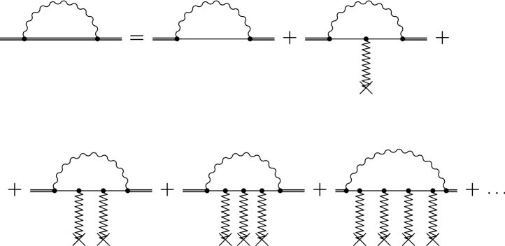
Figure 1: The figure illustrates the Feynman diagrams contributing to the high-energy part of the bound-electron self energy of a quantum cyclotron state in magnetic interaction vertices. These correspond to ascending powers of the operator $\Gamma_{\rm T}$ as delineated in Eq. (44).

A further difficulty arises. In Fig. 1, the outer lines (outside of the self-energy loop) are still fully dressed by the external field; for hydrogenic bound states, one therefore uses the known solutions of the Dirac–Coulomb equation for the bispinors $|\Psi\rangle$ and $\langle\overline{\Psi}|$ that enter the diagram (see, e.g., Chap. 8 of Ref. Jentschura and Adkins (2022)). For the quantum cyclotron problem, the nonperturbative Dirac solutions have recently been analyzed in Ref. Jentschura and Adkins (2022). They read as follows,

$$\Psi(\vec{r})=\mathcal{N}\,\left(\begin{array}[]{c}\psi_{\mathrm{NR}}(\vec{r})\\[8.61108pt] \dfrac{\vec{\sigma}\cdot\vec{\pi}_{\rm T}}{E_{D}+m}\psi_{\mathrm{NR}}(\vec{r})\end{array}\right)\equiv\Psi_{\ell ns}(\vec{r})\,.$$ (47)

where $\psi_{\mathrm{NR}}$ is the nonrelativistic wave functions, and all symbols will be explained in the following. For the high-energy part, one notes, in particular, that the relativistic states are needed for the untransformed Dirac equation, i.e., in the form of four-component bispinors. Two-component solutions obtained after a Foldy-Wouthuysen transformation Zou et al. cannot be used as bra and ket vectors for the fully relativistic self-energy matrix element in the integrand of Eq. (IV.3). We use the relativistic states in an approximation where the axial motion is being neglected, i.e., in the leading order in the expansion in powers of $\xi_{\mathrm{m}}$ and $\xi_{z}$. The Dirac energy is

$$E_{\mathrm{D}}=m\sqrt{1+\frac{\omega_{c}}{m}\left(2n+s+1\right)}\,.$$ (48)

The nonrelativistic Landau level in the symmetric gauge can be separated into a spinor component $\chi_{s}$ and and a coordinate-space wave function,

$$\psi_{\rm NR}(\vec{r})= \;\psi_{\ell ns}(\vec{r})=\psi_{n\ell}(\vec{\rho})\,\chi_{s}\,,$$ (49a)

$$\vec{\rho}= \;x\,\hat{\mathrm{e}}_{x}+y\,\hat{\mathrm{e}}_{y}\,,$$ (49b)

$$\chi_{+1}= \;\left(\begin{array}[]{c}1\\ 0\end{array}\right)\,,\qquad\chi_{-1}=\left(\begin{array}[]{c}0\\ 1\end{array}\right)\,.$$ (49g)

The nonrelativistic coordinate-space wave function is given as (see Ref. Jentschura and Adkins (2022))

$$\psi_{n\ell}(\vec{\rho})= \;\frac{2^{-\tfrac{1}{2}(|n-\ell|+1)}}{\sqrt{\pi}\,{\tilde{a}}_{0}}\,\sqrt{\frac{\min(n,\ell)!}{\max(n,\ell)!}}\,\left(\frac{\rho}{{\tilde{a}}_{0}}\right)^{|n-\ell|}$$

$$\;\times\mathrm{i}^{|n-\ell|}\,L^{|n-\ell|}_{\min(n,\ell)}\left(\frac{1}{2}\,\left(\frac{\rho}{{\tilde{a}}_{0}}\right)^{2}\right)\,$$

$$\;\times\mathrm{e}^{\mathrm{i}(n-\ell)\varphi}\,\exp\left[-\frac{1}{4}\,\left(\frac{\rho}{{\tilde{a}}_{0}}\right)^{2}\right]\,.$$ (50)

Here, $\rho=|\vec{\rho}|$ and $\varphi=\arctan(y/x)$, and we use the associated Laguerre polynomials $L_{n}^{a}(x)$ in the conventions of Ref. Abramowitz and Stegun (1972). The magnetic Bohr radius is

$${\tilde{a}}_{0}=\sqrt{\frac{mc^{2}}{\hbar\omega_{c}}}\,\frac{\hbar}{mc}=\frac{\hbar}{\alpha_{c}mc}=\sqrt{\frac{\hbar}{|e|B_{\rm T}}}\,.$$ (51)

The wave functions $\psi_{\ell ns}(\vec{r})$ fulfill the Dirac equation

$$H_{D}\Psi_{\ell ns}= \;E_{D}\Psi_{\ell ns}\,,$$ (52a)

$$H_{D}= \;\vec{\alpha}\cdot\vec{\pi}^{\parallel}_{\rm T}+\beta m\,,\qquad\vec{\pi}^{\parallel}_{\rm T}=\vec{p}_{\parallel}-e\vec{A}_{\rm T}\,,$$ (52b)

$$\vec{p}_{\parallel}= \;p_{x}\,\hat{\rm e}_{x}+p_{y}\,\hat{\rm e}_{y}\,.$$ (52c)

Finally, we can give the normalization factor as

$$\mathcal{N}=\left[1+\frac{2mE_{\mathrm{NR}}}{(E_{\mathrm{D}}+m)^{2}}\right]^{-\frac{1}{2}}\,,\quad E_{\mathrm{NR}}=\frac{\omega_{c}}{2}\,\left(2n+s+1\right)\,.$$ (53)

The relativistic wave function $\Psi$ given in Eq. (47) is valid for vanishing axial frequency, i.e., to leading order in the expansion in the ratio $\omega_{z}/\omega_{c}$, and can thus be used in order to evaluate the high-energy part of the quantum cyclotron bound-state self energy in the leading order in the expansion in powers of $\omega_{z}/\omega_{c}$.

We employ analogous procedures as those that were used for the high-energy part of the self energy of bound states in hydrogenlike systems Jentschura and Pachucki (1996), and map the algebra of the quantum cyclotron states onto a computer algebra system Wolfram (1999). This enables us to evaluate the matrix elements of the vertex terms for the high-energy part, where we employ a noncovariant integration procedure for the virtual photon integration contour outlined in Sec. 3 of Ref. Jentschura et al. (1997). The final result for the high-energy part is (almost) state-independent (except for the obvious spin-dependence of the leading term) and reads

$$E^{(2)}_{\rm HEP}=\frac{\alpha}{\pi}\,s\,\omega_{c}+\frac{2\alpha}{3\,\pi}\,\left[\ln\biggl{(}\frac{m}{2\,\epsilon}\biggr{)}-\frac{13}{72}\right]\,\frac{\omega_{c}^{2}}{m}\,,$$ (54)

where $\epsilon$ is the (noncovariant) photon energy cutoff. The first term in $E^{(2)}_{\rm HEP}$ reproduces the leading anomalous-magnetic-moment correction $E^{(0)}_{\rm HEP}$ given in Eq. (40).

IV.4 Low–Energy Part

The appropriate reference state for the low-energy part is given by the nonrelativistic quantum cyclotron wave function indicated in Eq. (II). Employing the formalism outlined in Chap. 4 of Ref. Jentschura and Adkins (2022), we obtain the expression

$$E_{\rm LEP}=\frac{2\alpha}{3\,\pi}\,\int_{0}^{\epsilon}{\mathrm{d}}k\,k\,\\ \times\left<\psi_{k\ell ns}\left|\frac{\pi^{i}_{\mathrm{T}}}{m}\,\left(\frac{1}{E_{0}-H_{0}-k}+\frac{1}{k}\right)\,\frac{\pi^{i}_{\mathrm{T}}}{m}\right|\psi_{k\ell ns}\right>\,,$$ (55)

where $k=\omega$ is the angular frequency of the virtual photon, $\epsilon$ is the photon energy cutoff, and $|\psi\rangle=|\psi_{k\ell ns}\rangle$ is the reference state. The sum over $i=1,2,3$ is implied by the Einstein summation convention. We use the relation

$$\left<\psi\left|\frac{\pi_{\mathrm{T}}^{i}}{m}\,(H_{0}-E_{0})\,\frac{\pi_{\mathrm{T}}^{i}}{m}\right|\psi\right>=\frac{\omega_{c}^{2}}{m}\,,$$ (56)

which can be shown after expressing the Cartesian components of the kinetic-momentum operator in terms of raising and lowering operators of the cyclotron and magnetron motions Boulware et al. (1985); Brown and Gabrielse (1986); Wienczek et al. (2022); Jentschura (2023b, a). Notably, the matrix element given in Eq. (56) is state-independent. After an integration over the photon energy, the low-energy part is obtained as

$$E_{\rm LEP}=\frac{2\,\alpha}{3\,\pi}\,\frac{\omega_{c}^{2}}{m}\,\ln\left(\frac{\epsilon}{\alpha_{c}^{2}\,m}\right)-\frac{2\,\alpha}{3\,\pi}\,\mathcal{M}\,,$$ (57)

where the coefficient of the logarithmic term contains a logarithmic sum (Bethe logarithm) over the virtual excitations of the quantum cyclotron state,

$$\mathcal{M}=\left<\phi_{r}\left|\frac{\pi_{\mathrm{T}}^{i}}{m}\,(H_{0}-E_{0})\,\ln\left(\frac{\left|H_{0}-E_{0}\right|}{\alpha_{c}^{2}\,m}\right)\,\frac{\pi_{\mathrm{T}}^{i}}{m}\right|\phi_{r}\right>\\ =\frac{\omega_{\mbox{\scriptsize$(+)$}}^{3}\,\ln\left(\frac{\omega_{\mbox{\scriptsize$(+)$}}}{\omega_{c}}\right)-\omega_{\mbox{\scriptsize$(-)$}}^{3}\,\ln\left(\frac{\omega_{\mbox{\scriptsize$(-)$}}}{\omega_{c}}\right)}{m\,(\omega_{\mbox{\scriptsize$(+)$}}-\omega_{\mbox{\scriptsize$(-)$}})}+\frac{\omega_{z}^{2}}{2m}\,\ln\left(\frac{\omega_{z}}{\omega_{c}}\right)\,.$$ (58)

In the simplification of the expressions, the following identities prove to be extremely useful,

$$\omega_{\mbox{\scriptsize$(+)$}}-\omega_{\mbox{\scriptsize$(-)$}}= \;\sqrt{\omega_{c}^{2}-2\omega_{z}^{2}}\,,$$ (59)

$$2\,\omega_{\mbox{\scriptsize$(+)$}}\,\omega_{\mbox{\scriptsize$(-)$}}= \;\omega_{z}^{2}\,.$$ (60)

Furthermore, it is very interesting to observe that, in the limit $\omega_{z}\to 0$, which implies $\omega_{\mbox{\scriptsize$(+)$}}\to\omega_{c}$ and $\omega_{\mbox{\scriptsize$(-)$}}\to\omega_{c}$, the Bethe-logarithm matrix element $\mathcal{M}$ vanishes. The first nonvanishing contribution to $\mathcal{M}$ appears at order $\xi_{z}^{4}$.

IV.5 Self–Energy Shift

After adding the high- and low-energy contributions, the dependence on the photon energy cutoff $\epsilon$ cancels [see Eqs. (41), (54) and (57)]. The total self-energy shift $E_{\rm SE}$, up to order $\alpha\,\alpha_{c}^{4}m$, is obtained as follows,

$$E_{\rm SE}=E^{[1]}_{\rm HEP}+E^{[2]}_{\rm HEP}+E_{\rm LEP}=\sum_{i=1}^{6}\mathcal{T}_{i}\,,$$ (61)

where the six individual contributions (together with their respective expansion in powers of $\xi_{z}$) are

$$\mathcal{T}_{1}= \;\frac{\alpha}{\pi}\,s\,\omega_{c}=\frac{\alpha}{\pi}\,\alpha_{c}^{2}m\,s\,,$$ (62a)

$$\mathcal{T}_{2}= \;\frac{\alpha}{\pi}\,\alpha_{c}^{4}m\,\left[\frac{2}{3}\ln\left(\alpha_{c}^{-2}\right)-\frac{2}{3}\,\ln(2)-\frac{13}{108}\right]\,,$$ (62b)

$$\mathcal{T}_{3}= \;-\frac{\alpha}{8\pi}\frac{s\omega_{c}\omega_{z}}{m}(k+\tfrac{1}{2})=-\frac{\alpha}{8\pi}\alpha_{c}^{4}ms\,\xi_{z}^{2}\,(k+\tfrac{1}{2})\,,$$ (62c)

$$\mathcal{T}_{4}= \;-\frac{\alpha}{4\pi}\frac{\omega_{z}^{2}s}{m}\frac{\omega_{\mbox{\scriptsize$(+)$}}(n+\tfrac{1}{2})+\omega_{\mbox{\scriptsize$(-)$}}(\ell+\tfrac{1}{2})}{\omega_{\mbox{\scriptsize$(+)$}}-\omega_{\mbox{\scriptsize$(-)$}}}$$

$$= \;\frac{\alpha}{\pi}\alpha_{c}^{4}m\,\left[-\frac{1}{8}(2n+1)s\,\xi_{z}^{4}\right]+\mathcal{O}(\xi_{z}^{6})\,,$$ (62d)

$$\mathcal{T}_{5}= \;-\frac{\alpha}{3\,\pi}\,\frac{\omega_{z}^{2}}{m}\,\ln\left(\frac{\omega_{z}}{\omega_{c}}\right)$$

$$= \;\frac{\alpha}{\pi}\alpha_{c}^{4}m\,\left[-\frac{2}{3}\,\xi_{z}^{4}\,\ln(\xi_{z})\right]\,,$$ (62e)

$$\mathcal{T}_{6}= \;-\frac{2\,\alpha}{3\,\pi}\,\frac{\omega_{\mbox{\scriptsize$(+)$}}^{3}\,\ln\left(\frac{\omega_{\mbox{\scriptsize$(+)$}}}{\omega_{c}}\right)-\omega_{\mbox{\scriptsize$(-)$}}^{3}\,\ln\left(\frac{\omega_{\mbox{\scriptsize$(-)$}}}{\omega_{c}}\right)}{m(\omega_{\mbox{\scriptsize$(+)$}}-\omega_{\mbox{\scriptsize$(-)$}})}$$

$$= \;\frac{\alpha}{\pi}\alpha_{c}^{4}m\frac{\xi_{z}^{4}}{3}+\mathcal{O}(\xi_{z}^{6})\,.$$ (62f)

The leading (state-independent) logarithmic contribution to the Lamb shift of a quantum cyclotron state is

$$E_{L}=\frac{2\,\alpha}{3\,\pi}\,m\,\frac{\omega_{c}^{2}}{m^{2}}\,\ln\left(\alpha_{c}^{-2}\right)=\frac{2\,\alpha}{3\,\pi}\,\alpha_{c}^{4}\,m\,\ln\left(\alpha_{c}^{-2}\right)\,.$$ (63)

It is reassuring to see that the only state-dependent contributions to the QED energy shift of order $\alpha\,\alpha_{c}^{4}\,m$ come from the anomalous magnetic moment.

The final results of our investigations can be summarized in the following, concise form, encapsulating the leading coefficients in the self energy shift given in Eq. (24),

$$E_{\rm SE}=\frac{\alpha}{\pi}\,\alpha_{c}^{2}m\mathcal{A}_{20}+\frac{\alpha}{\pi}\,\alpha_{c}^{4}m\left[\mathcal{A}_{41}\,\ln(\alpha_{c}^{-2})+\mathcal{A}_{40}\right]\,,$$ (64a)

where the coefficients are, except for $$\mathcal{A}_{20} \xi_{z}$$, state-independent, and read as follows in the leading order of the expansion in powers of ,

$$\mathcal{A}_{20}= \;s\,,\qquad\mathcal{A}_{41}=\frac{2}{3}\,,$$ (64b)

$$\mathcal{A}_{40}= \;-\frac{2}{3}\ln(2)-\frac{13}{108}+\mathcal{O}(\xi_{z}^{2})\,,$$ (64c)

We also evaluate partial results for the dependence of the $\mathcal{A}_{40}$ coefficient on the axial frequency. These results are partial, because the treatment of the high-energy part of the self energy employed by us is valid only to leading order in $\xi_{z}$. The corrections evaluated by us add up to the partial higher-order (h.o.) result

$$\left.\mathcal{A}_{40}\right|_{\mbox{h.o.}}=\left.\mathcal{A}_{40}\right|_{\xi_{z}=0}-\frac{1}{8}\,\left(k+\frac{1}{2}\right)\,s\,\xi_{z}^{2}\\ +\left[\frac{1}{3}-\frac{1}{8}(2n+1)s-\frac{2}{3}\ln(\xi_{z})\right]\,\xi_{z}^{4}+\mathcal{O}(\xi_{z}^{6})\,.$$ (65)

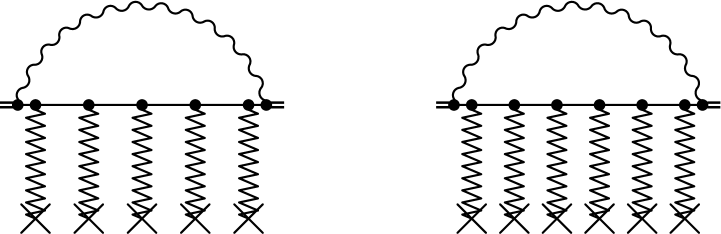
Figure 2: The diagrams with five magnetic vertices (left), and six magnetic vertices (right) contribute to the state-dependent, logarithmic term of order $\alpha\,\alpha_{c}^{6}m\,\ln(\alpha^{-2})$, as discussed in Eq. (66).

IV.6 Higher–Order Logarithmic Term

It is somewhat surprising to see that the coefficients $\mathcal{A}_{41}$ and $\mathcal{A}_{40}$ are state-independent in the leading order in the expansion in $\xi_{z}$. Because the axial frequency is small compared to the cyclotron frequency, this observation raises the question at which order in the expansion in $\alpha_{c}$ (i.e., in the main cyclotron frequency expansion parameter) any state dependence is actually incurred. With some effort, one can obtain the leading logarithmic terms in the sixth order in $\alpha_{c}$ from the six-vertex correction (see Fig. 2). We obtain, after algebraic simplification, the result

$$\delta E_{\rm SE}=\frac{\alpha}{\pi}\,\alpha_{c}^{6}m\,\mathcal{A}_{61}\,\ln(\alpha_{c}^{-2})\,,\quad\mathcal{A}_{61}=2n+1-\frac{4s}{3}\,.$$ (66)

This result depends on the spin orientation of the reference state, just like $\mathcal{A}_{20}$, and also grows with the principal quantum number $n$, which is the quantum number that counts the cyclotron excitations. Further details of the derivation will be presented elsewhere Jentschura (2023c).

For hydrogenic bound states, the higher-order coefficients typically decrease with the principal quantum number Le Bigot et al. (2003); for quantum cyclotron states, the dependence is reversed. The physical reason for this is that in hydrogen, higher excited states have a lesser expectation values of the momentum square, and are, in that sense, less relativistic and subjected to a lesser extent to relativistic and quantum electrodynamic corrections. Specifically, in a hydrogenic state with principal quantum number $n$, the typical momentum scale is $Z\alpha m/n$, where $Z$ is the nuclear charge number, $\alpha$ is the fine-structure constant, and $m$ is the electron mass. For a quantum cyclotron state, the momentum scale is $\alpha_{c}\,m\,\sqrt{n}$, where $\alpha_{c}$ is defined in Eq. (1). So, it is natural that $\mathcal{A}_{61}$ increases with the quantum cyclotron quantum number $n$.

V Conclusions

In this paper, we have discussed the QED energy shifts of quantum cyclotron levels. We start from a very concise recap of the main ingredients of quantum cyclotron levels in Sec. II, with vacuum-polarization effects discussed in Sec. III and the dominant self-energy shift discussed in Sec. IV. In the Penning trap, the rotational symmetry of the hydrogen and atomic bound-state problem is lost, and only the axial symmetry of the magnetic trap field remains. Hence, one formulates the bound states using spin-up and spin-down fundamental spinors [see Eq. (II)], rather than the spin-angular functions known from atomic bound-state theory (see Chap. 6 of Ref. Jentschura and Adkins (2022)).

The kinetic momentum operator $\vec{\pi}_{\mathrm{T}}$ given in Eq. (9) can easily be decomposed into raising and lowering operators for the cyclotron, axial, and magnetron motions. Hence, one can express the matrix elements of the radiatively corrected relativistic Hamiltonian given in Eq. (38) in terms of the quantum numbers $k$, $\ell$, $n$ and $s$ (see also Refs. Boulware et al. (1985); Brown and Gabrielse (1986); Wienczek et al. (2022); Jentschura (2023b, a)). One adds the high-energy contribution due to the anomalous magnetic moment from Eq. (41), and the high-energy contribution from the terms with up to four magnetic vertices, as given in Eq. (54), to the low-energy term listed in Eq. (57). The complete self-energy shift of order $\alpha\,\alpha_{c}^{4}\,m$ is given in Eq. (61). By considering diagrams with up to six magnetic vertices (see Fig. 2), as a significant further result, one obtains a state-dependent, higher-order logarithmic binding correction of order $\alpha\,\alpha_{c}^{6}\,m\ln(\alpha_{c}^{-2})$ in Eq. (66).

A few words on the experimental and phenomenological relevance of the higher-order binding corrections calculated here are in order. Because of the scaling with higher powers of the coupling parameter $\alpha_{c}$, the effects become more pronounced in stronger magnetic fields. In current Penning trap experiments Fan et al. (2023), field strengths of the order of $B_{\rm T}\approx 5.3\,{\rm T}$ are employed, resulting in $\omega_{c}\approx 2\pi\times 148\,{\rm GHz}$ and cyclotron coupling parameter $\alpha_{c}\approx 3.5\times 10^{-5}$, which implies $\ln[\alpha_{c}^{-2}]\approx 20.5$. With an axial frequency of the order of $\omega_{z}\approx 2\pi\times 114\,{\rm MHz}$, one has $\xi_{z}\approx 0.028$.

The higher-order one-loop binding corrections to the quantum cyclotron energy levels calculated here scale as follows. We have in the fourth order in $\alpha_{c}$, from Eq. (64a),

$$\delta E^{(4)}=\frac{\alpha}{\pi}\,\alpha_{c}^{4}m\left[\mathcal{A}_{41}\,\ln(\alpha_{c}^{-2})+\mathcal{A}_{40}\right]\,,$$ (67)

where the coefficients $\mathcal{A}_{41}$ and $\mathcal{A}_{40}$ are state-independent in the leading order in the expansion in $\xi_{z}$ [see Eqs. (64b) and (64c)]. Quantum cyclotron levels are displaced from each other by an energy $\omega_{c}=\alpha_{c}^{2}m$. Hence, the relative shift of the cyclotron frequency due to the quantum electrodynamic effects is

$$\chi^{(4)}\sim\frac{\delta E^{(4)}}{\alpha_{c}^{2}\,m}\,,\qquad\chi^{(4)}=\frac{\alpha}{\pi}\,\alpha_{c}^{2}\ln(\alpha_{c}^{-2})\,.$$ (68)

The nonlogarithmic coefficient $\mathcal{A}_{40}$ receives corrections of order $\xi_{z}^{2}$ according to Eq. (65). Parametrically, these additional terms lead to a relative energy shift of the order of $\chi^{(z)}$, where

$$\chi^{(z)}=\frac{\alpha}{\pi}\,\alpha_{c}^{2}\,\xi_{z}^{2}$$ (69)

for quantum cyclotron levels. Finally, the higher-order binding corrections given in Eq. (61) gives rise to a relative energy shift described by the parameter $\chi^{(6)}$, where

$$\chi^{(6)}=\frac{\alpha}{\pi}\,\alpha_{c}^{4}\,\ln(\alpha_{c}^{-2})\,.$$ (70)

For $B_{\rm T}\approx 5.3\,{\rm T}$ and $\omega_{z}\approx 2\pi\times 114\,{\rm MHz}$, i.e., the parameters of Ref. Fan et al. (2023), one has

$$\left.\chi^{(4)}\right|_{B_{T}=5.3\,{\rm T}}= \;5.8\times 10^{-11}\,,$$ (71)

$$\left.\chi^{(z)}\right|_{B_{T}=5.3\,{\rm T}}= \;2.1\times 10^{-15}\,,$$ (72)

$$\left.\chi^{(6)}\right|_{B_{T}=5.3\,{\rm T}}= \;6.9\times 10^{-20}\,.$$ (73)

In view of these results, we can say that the absence of a state-dependence of $\mathcal{A}_{41}$ and $\mathcal{A}_{40}$ (in the leading order in $\xi_{z}$) is crucial for the validity of the evaluation of the recent experiment Fan et al. (2023), as any dependence on $n$ could have easily shifted the determination of the cyclotron frequency (and of the electron $g$ factor) on the level of $10^{-11}$, which is larger than the experimental uncertainty reported in Ref. Fan et al. (2023) by roughly two orders of magnitude. The absence of a state-dependence of $\mathcal{A}_{41}$ and $\mathcal{A}_{40}$, in the leading order in $\xi_{z}$, is one of the most important results of the current investigation.

The corrections parameterized by $\chi^{(z)}$ and $\chi^{(6)}$ are not relevant at current experimental conditions Fan et al. (2023). However, according to Table 1 of Ref. Battesti et al. (2018), it is clear that magnetic field strengths in excess of $30\,{\rm T}$ are current maintained in continuous (DC) mode by a number of laboratories around the World. One of the most impressive results available to date is the $45.5\,{\rm T}$ field reported in Ref. Hahn et al. (2019). It is thus instructive to carry out calculations for a magnetic field of $B_{\rm T}=30\,{\rm T}$, with the results

$$\left.\chi^{(4)}\right|_{B_{T}=30\,{\rm T}}= \;3.0\times 10^{-10}\,,$$ (74)

$$\left.\chi^{(z)}\right|_{B_{T}=30\,{\rm T}}= \;2.1\times 10^{-15}\,,$$ (75)

$$\left.\chi^{(6)}\right|_{B_{T}=30\,{\rm T}}= \;2.0\times 10^{-18}\,.$$ (76)

For these conditions, the correction of order $\alpha\,\alpha_{c}^{6}\,\ln[\alpha_{c}^{-2}]$ could become relevant, when experimental techniques are combined with modern spectroscopic techniques Predehl et al. (2013). It is also very important to realize that state-dependent coefficients grow linearly with the cyclotron quantum number $n$, and axial quantum number $k$ [see Eqs. (65) and (66)]. The corrections thus become much more important for higher excited cyclotron states. We also observe that the mass $m$ of the trapped particle cancels out in the relative corrections denoted by the symbols $\chi^{(4)}$, $\chi^{(z)}$, and $\chi^{(6)}$, discussed above; in other words, the quantities $\chi^{(4)}$, $\chi^{(z)}$, and $\chi^{(6)}$ are functions of the coupling parameter $\alpha_{c}$ only. For given magnetic field, the coupling parameter $\alpha_{c}$ is inversely proportional to the trapped particle mass $m$ [see Eq. (1)], in view of the relation $\alpha_{c}=\sqrt{|e|B_{\mathrm{T}}}/m$. Hence, for hydrogen-like and lithium-like bound systems (ions) in a Penning trap, the quantum electrodynamic effects scale according to the dependence of $\alpha_{c}$ on the mass of the trapped ion.

Three final remarks are in order. (i) First, we reemphasize that vacuum-polarization contributions can be safely neglected, as already discussed near the beginning of Sec. III. (ii) Second, we would like to remind the reader that modifications of the QED shifts due to the cylinder walls of the Penning trap Boulware et al. (1985); Jentschura (2023b) have not been considered in the current work. We here work with the full photon propagator that is unperturbed by the external conditions due to the cylinder walls of the Penning trap. Because the average spatial extent of a quantum cyclotron state is only a tiny fraction of the trap dimension, this approximation is well justified, with limitations being discussed in Refs. Boulware et al. (1985); Jentschura (2023b). (iii) Relativistic Bethe logarithm corrections to the leading one-loop terms are of order self-energy shift of order $\alpha\,\alpha_{c}^{6}\,m$ while the correction obtained in Eq. (66) is enhanced by the logarithm $\ln(\alpha_{c}^{-2})$. The evaluation of relativistic Bethe logarithms, for quantum cyclotron states complementing work on hydrogenic levels Pachucki (1993); Jentschura and Pachucki (1996), would be an inspiration for future studies Jentschura (2023c).

References

- Brown and Gabrielse (1982) L. S. Brown and G. Gabrielse, “Precision spectroscopy of a charged particle in an imperfect Penning trap,” Phys. Rev. A 25, 2423(R)–2425(R) (1982).
- Brown et al. (1985) L. S. Brown, G. Gabrielse, K. Helmerson, and J. Tan, “Cyclotron Motion in a Microwave Cavity: Possible Shifts of the Measured Electron Factor,” Phys. Rev. Lett. 55, 44–47 (1985).
- Brown and Gabrielse (1986) L. S. Brown and G. Gabrielse, “Geonium theory: Physics of a single electron or ion in a Penning trap,” Rev. Mod. Phys. 58, 233–311 (1986).
- (4) B. Odom, D. Hanneke, B. D’Urso, and G. Gabrielse, New Measurement of the Electron Magnetic Moment Using a One–Electron Quantum Cyclotron, Phys. Rev. Lett. 97, 030801 (2006); G. Gabrielse, D. Hanneke, T. Kinoshita, M. Nio, and B. Odom, New Determination of the Fine Structure Constant from the Electron Value and QED, ibid. 97, 030802 (2006); Erratum: New Determination of the Fine Structure Constant from the Electron Value and QED [Phys. Rev. Lett. 97, 030802 (2006)], 99, 039902(E) (2007).
- Hanneke et al. (2008) D. Hanneke, S. Fogwell, and G. Gabrielse, “Measurement of the Electron Magnetic Moment and the Fine Structure Constant,” Phys. Rev. Lett. 100, 120801 (2008).
- Fan et al. (2023) X. Fan, T. G. Myers, B. A. D. Sukra, and G. Gabrielse, “Measurement of the Electron Magnetic Moment,” Phys. Rev. Lett. 130, 071801 (2023).
- Wienczek et al. (2022) A. Wienczek, C. Moore, and U. D. Jentschura, “Foldy–Wouthuysen transformation in strong magnetic fields and relativistic corrections for quantum cyclotron energy levels,” Phys. Rev. A 106, 012816 (2022).
- Bethe (1947) H. A. Bethe, “The Electromagnetic Shift of Energy Levels,” Phys. Rev. 72, 339–341 (1947).
- Pachucki (1993) K. Pachucki, “Higher-Order Binding Corrections to the Lamb Shift,” Ann. Phys. (N.Y.) 226, 1–87 (1993).
- Jentschura and Pachucki (1996) U. Jentschura and K. Pachucki, “Higher-order binding corrections to the Lamb shift of states,” Phys. Rev. A 54, 1853–1861 (1996).
- Uehling (1935) E. A. Uehling, “Polarization Effects in the Positron Theory,” Phys. Rev. 48, 55 (1935).
- Jentschura (2011a) U. D. Jentschura, “Lamb Shift in Muonic Hydrogen. —I. Verification and Update of Theoretical Predictions,” Ann. Phys. (N.Y.) 326, 500–515 (2011a).
- Jentschura (2011b) U. D. Jentschura, “Relativistic Reduced–Mass and Recoil Corrections to Vacuum Polarization in Muonic Hydrogen, Muonic Deuterium and Muonic Helium Ions,” Phys. Rev. A 84, 012505 (2011b).
- Jentschura et al. (1997) U. D. Jentschura, G. Soff, and P. J. Mohr, “Lamb shift of 3P and 4P states and the determination of ,” Phys. Rev. A 56, 1739–1755 (1997).
- Jentschura and Adkins (2022) U. D. Jentschura and G. S. Adkins, Quantum Electrodynamics: Atoms, Lasers and Gravity (World Scientific, Singapore, 2022).
- Schwinger (1948) J. Schwinger, “On Quantum-Electrodynamics and the Magnetic Moment of the Electron,” Phys. Rev. 73, 416–417 (1948).
- Baranger et al. (1953) M. Baranger, H. A. Bethe, and R. P. Feynman, “Relativistic Correction to the Lamb Shift,” Phys. Rev. 92, 482 (1953).
- Feynman (1949) R. P. Feynman, “Space–Time Approach to Quantum Electrodynamics,” Phys. Rev. 76, 769–789 (1949).
- Jentschura and Pachucki (2002) U. D. Jentschura and K. Pachucki, “Two–Loop Self–Energy Corrections to the Fine Structure,” J. Phys. A 35, 1927–1942 (2002).
- Schwinger (1949) J. Schwinger, “On Radiative Corrections to Electron Scattering,” Phys. Rev. 75, 898–899 (1949).
- Jentschura (2023a) U. D. Jentschura, “Algebraic Approach to Relativistic Landau Levels in the Symmetric Gauge,” Phys. Rev. D 108, 016016 (2023a).
- (22) L. Zou, P. Zhang, and A. J. Silenko, Production of twisted particles in magnetic fields, e-print arXiv:2207.14105v1.
- Abramowitz and Stegun (1972) M. Abramowitz and I. A. Stegun, Handbook of Mathematical Functions, 10th ed. (National Bureau of Standards, Washington, D. C., 1972).
- Wolfram (1999) S. Wolfram, The Mathematica Book, 4th ed. (Cambridge University Press, Cambridge, UK, 1999).
- Boulware et al. (1985) D. G. Boulware, L. S. Brown, and T. Lee, “Apparatus-dependent contributions to ?” Phys. Rev. D 32, 729–735 (1985).
- Jentschura (2023b) U. D. Jentschura, “Apparatus–Dependent Corrections to Revisited,” Phys. Rev. D 107, 076014 (2023b).
- Jentschura (2023c) U. D. Jentschura, in preparation (2023c).
- Le Bigot et al. (2003) E.-O. Le Bigot, U. D. Jentschura, P. J. Mohr, P. Indelicato, and Gerhard Soff, “Perturbation Approach to the self-energy of non- hydrogenic states,” Phys. Rev. A 68, 042101 (2003).
- Battesti et al. (2018) R. Battesti, J. Beard, S. Böser, N. Bruyant, D. Budker, S. A. Crooker, E. J. Daw, V. V. Flambaum, T. Inada, I. G. Irastorza, F. Karbstein, D. L. Kim, M. G. Kozlov, Z. Melhem, A. Phipps, P. Pugnat, G. Rikken, C. Rizzo, M. Schott, Y. K. Semertzidis, H. H. J. ten Kate, and G. Zavattini, “High magnetic fields for fundamental physics,” Phys. Rep. 765-766, 1–39 (2018).
- Hahn et al. (2019) S. Hahn, K. Kim, K. Kim, X. Hu, T. Painter, I. Dixon, S. Kim, K. R. Bhattarai, S. Noguchi, J. Jaroszynski, and D. C. Larbalestier, “45.5-tesla direct-current magnetic field generated with a high-temperature superconducting magnet,” Nature (London) 570, 496–502 (2019).
- Predehl et al. (2013) K. Predehl, G. Grosche, S. F. F. Raupach, S. Droste, O. Terra, J. Alnis, Th. Legero, T. W. Hänsch, Th. Udem, R. Holzwarth, and H. Schnatz, “A 920-Kilometer Optical Fiber Link for Frequency Metrology at the 19th Decimal Place,” Science 336, 441–444 (2013).