Quantum-noise-limited optical neural networks operating at a few quanta per activation

Abstract

Analog physical neural networks, which hold promise for improved energy efficiency and speed compared to digital electronic neural networks, are nevertheless typically operated in a relatively high-power regime so that the signal-to-noise ratio (SNR) is large (>10). What happens if an analog system is instead operated in an ultra-low-power regime, in which the behavior of the system becomes highly stochastic and the noise is no longer a small perturbation on the signal? In this paper we study this question in the setting of optical neural networks operated in the limit where some layers use only a single photon to cause a neuron activation. Neuron activations in this limit are dominated by quantum noise from the fundamentally probabilistic nature of single-photon detection of weak optical signals. We show that it is possible to train stochastic optical neural networks to perform deterministic image-classification tasks with high accuracy in spite of the extremely high noise (SNR $\sim$ 1) by using a training procedure that directly models the stochastic behavior of photodetection. We experimentally demonstrated MNIST handwritten-digit classification with a test accuracy of $98\%$ using an optical neural network with a hidden layer operating in the single-photon regime; the optical energy used to perform the classification corresponds to 0.008 photons per multiply–accumulate (MAC) operation, which is equivalent to 0.003 attojoules of optical energy per MAC. Our experiment used >40$\times$ fewer photons per inference than previous state-of-the-art low-optical-energy demonstrations, to achieve the same accuracy of >90%. Our work shows that some extremely stochastic analog systems, including those operating in the limit where quantum noise dominates, can nevertheless be used as layers in neural networks that deterministically perform classification tasks with high accuracy if they are appropriately trained.

I Introduction

The development and widespread use of very large neural networks for artificial intelligence [1, 2, 3] has motivated the exploration of alternative computing paradigms—including analog processing—in the hope of improving both energy efficiency and speed [4, 5]. Photonic implementations of neural networks using analog optical systems have experienced a resurgence of interest over the past several years [6, 7, 8, 9, 10, 11, 12, 13, 14, 15, 16, 17]. However, analog processors—including those constructed using optics—inevitably have noise and typically also suffer from imperfect calibration and drift. These imperfections can result in degraded accuracy for neural-network inference performed using them [6, 18, 19, 20]. To mitigate the impact of noise, noise-aware training schemes have been developed [21, 22, 23, 24, 25, 26, 27, 28, 29]. These schemes treat the noise as a relatively small perturbation to an otherwise deterministic computation, either by explicitly modeling the noise as the addition of random variables to the processor’s output or by modeling the processor as having finite bit precision. Recent demonstrations of ultra-low optical energy usage in optical neural networks (ONNs) [13, 16] were in this regime of noise as a small perturbation and used hundreds to thousands of photons to represent the average neuron pre-activation signal prior to photodetection. In Ref. [13], we reported achieving $90\%$ accuracy on MNIST handwritten-digit classification using slightly less than 1 photon per scalar weight multiplication (i.e., per MAC)—which is already counterintuitively small—and one might be tempted to think that it’s not possible to push the number of photons per MAC much lower while preserving accuracy. More typically, millions of photons per activation are used [11, 12, 16, 30]. In this paper we address the following question: what happens if we use such weak optical signals in a ONN that each photodetector in a neural-network layer receives at most just one, or perhaps two or three, photons?

Physical systems are subject to various sources of noise. While some noise can be reduced through improvements to the hardware, some noise is fundamentally unavoidable, especially when the system is operated with very little power—which is an engineering goal for neural-network processors. Shot noise is a fundamental noise that arises from the quantized, i.e., discrete, nature of information carriers: the discreteness of energy in the case of photons in optics, and of discreteness of charge in the case of electrons in electronics [31]. A shot-noise-limited measurement of a signal encoded with an average of $N_{\textrm{p}}$ photons (quanta) will have an SNR that scales as $\sqrt{N_{\textrm{p}}}$ [32]. To achieve a suitably high SNR, ONNs typically use a large number of quanta for each detected signal. In situations where the optical signal is limited to just a few photons, photodetectors measure and can count individual quanta. Single-photon detectors (SPDs) are highly sensitive detectors that—in the typical click detector setting—report, with high fidelity, the absence of a photon (no click) or presence of one or more photons (click) during a given measurement period [34]. In the quantum-noise-dominated regime of an optical signal with an average photon number of about 1 impinging on an SPD, the measurement outcome will be highly stochastic, resulting in a very low SNR (of about 1). Conventional noise-aware-training algorithms are not able to achieve high accuracy with this level of noise. Is it possible to operate ONNs in this very stochastic regime and still achieve high accuracy in deterministic classification tasks? The answer is yes, and in this work we will show how.

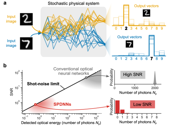
Figure 1: Deterministic inference using noisy neural-network hardware. a, The concept of a stochastic physical neural network performing a classification task. Given a particular input image to classify, repetitions exhibits variation (represented by different traces of the same color), but the class is predicted nearly deterministically. b, The single-to-noise ratio (SNR) of single-photon-detection neural networks (SPDNNs) compared to conventional optical neural networks (ONNs). Conventional ONNs operate with high photon budgets (SNR $\gg 1$) to obtain reliable results, whereas SPDNNs operate with low photon budgets—of up to just a few detected photons per shot (SNR $\sim 1$). The relation between the detected optical energy (in number of photons $N_{\textrm{p}}$) and SNR is SNR $=\sqrt{N_{\textrm{p}}}$, which is known as the shot-noise limit.

The stochastic operation of neural networks has been extensively studied in computer science as part of the broader field of stochastic computing [35]. In the field of machine learning, binary stochastic neurons (BSNs) have been used to construct stochastic neural networks [36, 37, 38, 39, 40, 41, 42], with training being a major focus of study. Investigations of hardware implementations of stochastic computing neural networks, such as those in Refs. [43, 44] (with many more surveyed in Ref. [45]), have typically been for deterministic complementary metal–oxide–semiconductor (CMOS) electronics, with the stochasticity introduced by random-number generators. While many studies of binary stochastic neural networks have been conducted with standard digital CMOS processors, there have also been proposals to construct them from beyond-CMOS hardware, motivated by the desire to minimize power consumption: direct implementation of binary stochastic neurons using bistable systems that are noisy by design—such as low-barrier magnetic tunnel junctions (MTJs)—has been explored [46, 47, 48], and there have also been proposals to realize hardware stochastic elements for neural networks that could be constructed with noisy CMOS electronics or other physical substrates [49, 50]. ONNs in which noise has been intentionally added [25, 51, 52] have also been studied. Our work with low-photon-count optics is related but distinct from many of the studies cited here in its motivating assumption: instead of desiring noise and stochastic behavior—and purposefully designing devices to have them, we are concerned with situations in which physical devices have large and unavoidable noise but where we would like to nevertheless construct deterministic classifiers using these devices because of their potential for low-energy computing (Figure 1).

The key idea in our work is that when ONNs are operated in the approximately-1-photon-per-neuron-activation regime and the detectors are SPDs, it is natural to consider the neurons as binary stochastic neurons: the output of an SPD is binary (click or no click) and fundamentally stochastic. Instead of trying to train the ONN as a deterministic neural network that has very poor numerical precision, one can instead train it as a binary stochastic neural network, adapting some of the methods from the last decade of machine-learning research on stochastic neural networks [39, 40, 41, 53, 42, 54, 45] and using a physics-based model of the stochastic single-photon detection (SPD) process during training. We call this physics-aware stochastic training.

We experimentally implemented a stochastic ONN using as a building block an optical matrix-vector multiplier [13] modified to have SPDs at its output: we call this a single-photon-detection neural network (SPDNN). We present results showing that high classification accuracy can be achieved even when the number of photons per neuron activation is approximately 1, and even without averaging over multiple shots. We also studied in simulation how larger, more sophisticated stochastic ONNs could be constructed and what their performance on CIFAR-10 image classification would be.

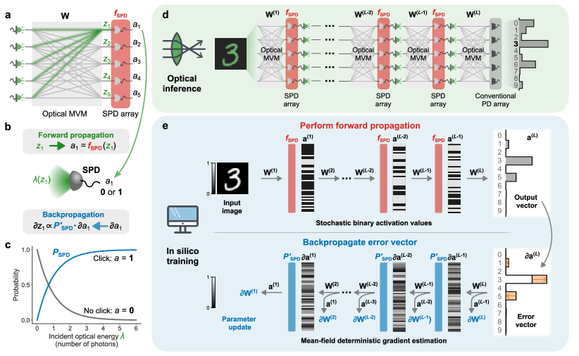
Figure 2: Single-photon-detection neural networks (SPDNNs): physics-aware stochastic training and inference. a, A single layer of an SPDNN, comprising an optical matrix-vector multiplier (optical MVM, in grey) and single-photon detectors (SPDs; in red), which perform stochastic nonlinear activations. Each output neuron’s value is computed by the physical system as $a_{i}=f_{\text{SPD}}(z_{i})$), where $z_{i}$ is the weighted sum (shown in green) of the input neurons to the $i$th output neuron computed as part of the optical MVM, and $a_{i}$ is the stochastic binary output from a single-photon detector. b, Forward and backward propagation through the SPD activation function. The optical energy ($\lambda$) incident on an SPD is a function of $z_{i}$ that depends on the encoding scheme used. Forward propagation uses the stochastic binary activation function $f_{\text{SPD}}$, while backpropagation involves the mean-field function of the probability $P_{\text{SPD}}$. c, Probability of an SPD detecting a click (output $a=1$) or not (output $a=0$), as a function of the incident light energy $\lambda$. d, Optical inference using an SPDNN with $L$ layers. The activation values from the SPD array of each layer are passed to light emitters for the optical MVM of the next layer. The last layer uses a conventional photodetector (PD) array instead of an SPD array, and is operated with enough optical energy that the output of this layer has high SNR. e, In silico training of an SPDNN with $L$ layers. Each forward propagation is stochastic, and during backpropagation, the error vector is passed to the hidden layers using the mean-field probability function $P_{\text{SPD}}$ instead of the stochastic activation function $f_{\text{SPD}}$. In this figure, $\partial x$ is shorthand for $\partial C/\partial x$, where $C$ is the cost function.

II Single-photon-detection neural networks: optical neural networks with stochastic activation from single-photon detection

We consider ONNs in which one or more layers are each constructed from an optical matrix-vector multiplier followed by an array of SPDs (Figure 2a–c), and in which the optical powers used are sufficiently low that in each execution of the layer, each SPD has at most only a few photons impinging on it, leading to stochastic measurement outcomes of no click or click.

In our setting, we aim to perform inference using the SPDNN—with its implementation in physical hardware—(Figure 2d) and to perform training of the SPDNN in silico (Figure 2e–f). That is, training is performed entirely using standard digital electronic computing.

II.1 Physics-aware stochastic training

To train an SPDNN, we perform gradient descent using backpropagation, which involves a forward pass, to compute the current error (or loss) of the network, and a backward pass, which is used to compute the gradient of the loss with respect to the network parameters; our procedure is inspired by backpropagation-based training of stochastic and binary neural networks [39, 42]. We model the forward pass (upper part of Figure 2e) through the network as a stochastic process that captures the key physics of SPD of optical signals having Poissonian photon statistics [55]: the measurement outcome of SPD is a binary random variable (no click or click) that is drawn from the Bernoulli distribution with a probability that depends on the mean photon number of the light impinging on the detector. However, during the backward pass (lower part of Figure 2e), we employ a deterministic mean-field estimator to compute the gradients. This approach avoids the stochasticity and binarization of the SPD process, which typically pose difficulties for gradient estimation.

We now give a brief technical description of our forward and backward passes for training; for full details see Methods and Supplementary Notes 1A and 2A. We denote the neuron pre-activations of the $l$th stochastic layer of an SPDNN as $\textbf{z}^{(l)}=W^{(l)}\textbf{a}^{(l-1)}$, where $\textbf{a}^{(l-1)}$ is the activation vector from the previous layer ($\textbf{a}^{(0)}$ denotes the input vector x of the data to be classified). In the physical realization of an SPDNN, $\textbf{z}^{(l)}$ is encoded optically (for example, in optical intensity) following an optical matrix-vector multiplier (optical MVM, which computes the product between the matrix $W^{(l)}$ and the vector $\textbf{a}^{(l-1)}$) but before the light impinges on an array of SPDs. We model the action of an SPD with a stochastic activation function, $f_{\text{SPD}}$ (Figure 2b; Eq. 1). The stochastic output of the $l$th layer is then $\textbf{a}^{(l)}=f_{\text{SPD}}(\textbf{z}^{(l)})$.

For an optical signal having mean photon number $\lambda$ and that obeys Poissonian photon statistics, the probability of a click event by an SPD is $P_{\text{SPD}}(\lambda)=1-e^{\lambda}$ (Figure 2c). We define the stochastic activation function $f_{\text{SPD}}$ as follows:

$$f_{\text{SPD}}(z)\coloneqq\begin{cases}1&\text{with probability $p=P_{\text{SPD}}(\lambda(z))$},\\ 0&\text{with probability $1-p$,}\end{cases}$$ (1)

where $\lambda(z)$ is a function mapping a single neuron’s pre-activation value to a mean photon number. For an incoherent optical setup where the information is directly encoded in intensity, $\lambda(z)=z$; for a coherent optical setup where the information is encoded in field amplitude and the SPD directly measures the intensity, $\lambda(z)=|z|^{2}$. In general, the form of $\lambda(z)$ is determined by the signal encoding used in the optical MVM, and the detection scheme following the MVM. We use $f_{\text{SPD}}$ in modeling the stochastic behavior of an SPDNN layer in the forward pass. However, during the backward pass, we make a deterministic mean-field approximation of the network: instead of evaluating the stochastic function $f_{\text{SPD}}$, we evaluate $P_{\text{SPD}}(\lambda(z))$ when computing the activations of a layer: $\textbf{a}^{(l)}=P_{\text{SPD}}(\lambda(\textbf{z}^{(l)}))$ (Figure 2b). This is an adaptation of a standard machine-learning method for computing gradients of stochastic neural networks [39].

II.2 Inference

When performing inference (Figure 2d), we can run just a single shot of a stochastic layer or we can choose to take the average of multiple shots—trading greater energy and/or time usage for reduced stochasticity. For a single shot, a neuron activation takes on the value $a^{[1]}=a\in\{0,1\}$; for $K$ shots, $a^{[K]}=\frac{1}{K}\sum^{K}_{k=1}a_{k}\in\{0,1/K,2/K,\ldots,1\}$. In the limit of infinitely many shots, $K\rightarrow\infty$, the activation $a^{[\infty]}$ would converge to the expectation value, $a^{[\infty]}=\mathbb{E}[a]=P_{\text{SPD}}(\lambda(z))$. In this work we focus on the single-shot ($K=1$) and few-shot $K\leq 5$ regime, since the high-shot $K\gg 100$ regime is very similar to the high-photon-count-per-shot regime that has already been studied in the ONN literature (e.g., in Ref. [13]). An important practical point is that averaging for $K>1$ shots can be achieved by counting the clicks from each SPD, which is what we did in the experiments we report. We can think of $K$ as a discrete integration time, so averaging need not involve any data reloading or sophisticated control.

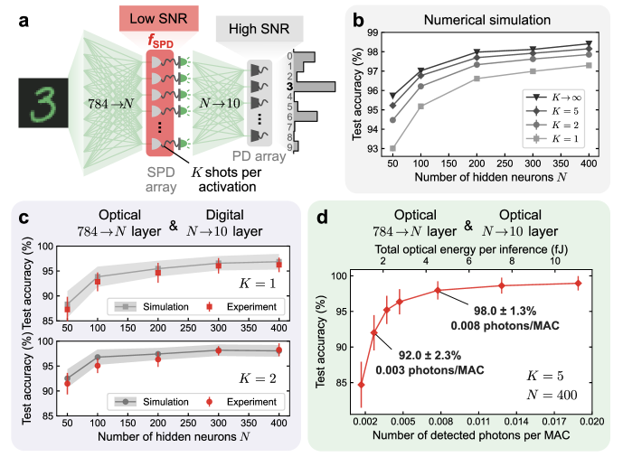
Figure 3: Performance of a single-photon-detection neural network (SPDNN) on MNIST handwritten-digit classification. a, An SPDNN realizing a multilayer perceptron (MLP) architecture of $N$ neurons in the hidden layer. The hidden layer ($784\rightarrow N$) was computed using an incoherent optical matrix-vector-multiplier (MVM) followed by a single-photon-detector (SPD) array. Each SPD realized a stochastic activation function for a single hidden-layer neuron. During a single inference, the hidden layer was executed a small number of times ($1\leq K\leq 5$), yielding averaged activation values. The output layer ($N\rightarrow 10$) was realized either optically—using an optical MVM and high photon budget to achieve high readout SNR, as in conventional ONNs, or with a digital electronic processor, yielding a result with full numerical precision. b, Simulated test accuracy of MNIST handwritten-digit classification for models with different numbers of hidden neurons $N$ and shots per activation $K$. Each activation value is obtained by averaging $K$ shots of stochastic binary SPD readouts. When $K\rightarrow\infty$, the stochastic activations $a_{i}$ become the expectations $\mathbb{E}[a_{i}]$, which are deterministic. The test accuracy with few shots is close to the accuracy achieved in the deterministic limit. c, Experimental evaluation of the SPDNN, with the output layer performed with full numerical precision on a digital computer. Results are presented for both $K=1$ (single-shot, i.e., no averaging; top) and $K=2$ (bottom) shots per activation. d, Experimental evaluation of the SPDNN, with both the hidden and the output layer executed using the optical experimental apparatus. The average number of detected photons used per inference in the hidden layer was kept fixed and the number used per inference in the output layer was varied (see main text for numbers). The number of detected photons per inference is reported both as an aggregate optical energy (top axis) and as a per-MAC quantity (bottom axis), which we obtained by dividing the number of photons per inference by the number of MACs performed in a single inference. The mean and standard deviation of the test accuracy were estimated used 100 repetitions of inference for each image in the test set.

III MNIST handwritten-digit classification with a single-photon-detection multilayer perceptron

We evaluated the performance—both in numerical simulations and in optical experiments—of SPDNNs on the MNIST handwritten-digit-classification benchmark task with a simple, $784\rightarrow N\rightarrow 10$ multilayer perceptron (MLP) architecture (Figure 7a). The activation values in the hidden layer were computed by SPDs. The optical power was chosen so that the SNR of the SPD measurements was $\sim 1$, falling in the low-SNR regime (Figure 1b). The output layer was implemented either with full numerical precision on a digital electronic computer, or optically with an integration time set so that the measured signal comprised enough photons that a high SNR (Figure 1b) was achieved, as in conventional ONNs. Our use of a full-precision output layer is consistent with other works on binary neural networks [42, 56, 57]. In a shallow neural network, executing the output layer at high SNR substantially limits the overall energy efficiency gains from using small photon budgets in earlier layers, but in larger models, the relatively high energy cost of a high-SNR output layer is amortized. Nevertheless, as we will see, even with just a single-hidden-layer network, efficiency gains of >40$\times$ are possible by performing the hidden layer in the low-SNR regime.

The models we report on in this section used non-negative weights in the hidden layers and real-valued weights in the output layers. This allows the hidden layers to be straightforwardly realized with optical MVMs using incoherent light. In Section IV and Supplementary Note 2, we report on extensions to the case of real-valued weights in coherent optical processors.

III.1 Simulation results

First, we digitally simulated the SPDNN models shown in Figure 7a. We report the simulated test accuracies in Figure 7b for the full test dataset of 10,000 images, as a function of the number of hidden neurons $N$ and the number of shots $K$ of binary SPD measurements integrated to compute each activation.

Due to the stochastic nature of the model, the classification output for a fixed input varies from run to run. We repeated inferences on fixed inputs from the test set 100 times; we report the mean and standard deviation of the test accuracy as data points and error bars, respectively. The standard deviations of the test accuracies are around $0.1\%$.

The accuracy achieved by the SPDNN is substantially higher than for linear models ($<93\%$ classification accuracy on MNIST [59]). This both shows that despite the hidden layer being stochastic, high-accuracy determistic classification is possible, and that the SPD activation function serves as a suitable nonlinearity in the neural network. The sizes of the models we simulated (in number of neurons $N$) are similar to those of traditional deterministic neural networks for MNIST classification [60], so the high accuracies achieved are not a simple consequence of averaging over many noisy neurons [61].

If we integrated an infinite number of SPD measurements for each activation ($K\rightarrow\infty$)—which is infeasible in experiment, but can be simulated—then the SPDNN output would become deterministic. The test accuracy achieved in this limit can be considered as an upper bound, as the classification accuracy improves monotonically with $K$. Notably, even with just a single SPD measurement ($K=1$) for each activation, the mean test accuracy is around $97\%$. The accuracy is substantially improved with just a few more shots of averaging, and approaches the deterministic upper bound when $K\gtrsim 5$. The mean single-photon-detection probability, averaged over all neurons, is $\approx 0.5$, so the simulated number of detected photons per shot is very small: $\approx 0.5N$. As we will quantify in the next section reporting the results of optical experiments, this means high accuracy can be achieved using much less optical energy than in conventional ONNs.

III.2 Optical experimental results

In our experimental demonstrations, we based our SPDNN on a free-space optical matrix-vector multiplier (MVM) that we had previously constructed for high-SNR experiments [13], and replaced the detectors with SPDs so that we could operate it with ultra-low photon budgets (see Methods). The experiments we report were, in part, enabled by the availability of cameras comprising large arrays of pixels capable of detecting single photons with low noise [62]. We encoded neuron values in the intensity of incoherent light; as a result, the weights and input vectors were constrained to be non-negative. However, this is not a fundamental feature of SPDNNs—in the next section (Section IV), we present simulations of coherent implementations that lift this restriction. A single-photon-detecting camera measured the photons transmitted through the optical MVM, producing the stochastic activations as electronic signals that were input to the following neural-network layer (see Methods and Supplementary Note 3 and 4).

In our first set of optical experiments, the hidden layer was realized optically and the output layer was realized in silico (Figure 7c): the output of the SPD measurements after the optical MVM was passed through a linear classifier executed with full numerical precision on a digital electronic computer. We tested using both $K=1$ (no averaging) and $K=2$ shots of averaging the stochastic binary activations in the hidden layer. The results agree well with simulations, which differ from the simulation results shown in Figure 7b because they additionally modeled imperfections in our experimental optical-MVM setup (see Methods, Supplementary Note 7). The test accuracies were calculated using 100 test images, with inference for each image repeated 30 times. The hidden layer (the one computed optically in these experiments) used approximately 0.0008 detected photons per MAC, which is $\geq 6$ orders of magnitude lower than is typical in ONN implementations [11, 12, 16, 30] and $\geq 3$ orders of magnitude lower than the lowest photons-per-MAC numbers reported to date [13, 16].

We then performed experiments in which both the hidden layer and the output layer were computed optically (Figure 7d). In these experiments, we implemented a neural network with 400 hidden neurons and used 5 shots per inference ($N=400$, $K=5$). The total optical energy was varied by changing the number of photons used in the output layer; the number of photons used in the hidden layer was kept fixed.

The average value of the stochastic binary activations $a_{i}$ in the hidden layer was $\approx 0.522$. This corresponds to a total of $0.522\times N\times K=1044$ photons being detected in the hidden layer per inference. The total detected optical energy per inference comprises the sum of the detected optical energy in the hidden ($784\rightarrow 400$) layer and in the output ($400\rightarrow 10$) layer (see Methods, Supplementary Table 6 and Supplementary Note 9).

The results show that even though the output layer was operated in the high-SNR regime (Figure 1b), the full inference computation achieved high accuracy yet used only a few femtojoules of optical energy in total (equivalent to a few thousand photons). By dividing the optical energy by the number of MACs performed in a single inference, we can infer the per-MAC optical energy efficiency achieved: with an average detected optical energy per MAC of approximately 0.001 attojoules (0.003 attojoules), equivalent to 0.003 photons (0.008 photons), the test accuracy was $92.0\pm 2.3\%$ ($98.0\pm 1.3\%$).

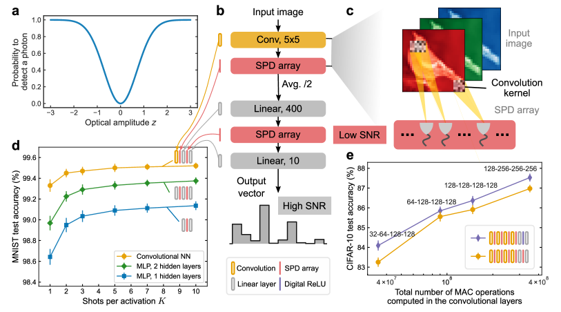
Figure 4: Simulation study predicting the performance of proposed coherent single-photon-detection neural networks (SPDNNs). a, The probability of detecting a photon as a function of the input light amplitude in a coherent SPDNN. Real-valued numbers are encoded in coherent light with either 0 phase (positive numbers) or $\pi$ phase (negative numbers). Measurement by a single-photon detector (SPD) results in the probabilistic detection of a photon that is proportional to the square of the encoded value $z$, in comparison to intensity encodings with incoherent light. b, Structure of a convolutional SPDNN with a kernel size of $5\times 5$. Single-shot SPD measurements ($K=1$) are performed after each layer (by an SPD array), except for the output layer. Average $2\times 2$ pooling is applied after each convolutional operation. A digital rectified linear unit (ReLU) [63] activation function can also be used in the linear layer as an alternative. c, Schematic of a convolutional layer with SPD activations. d, Simulated test accuracy of coherent SPDNNs with varying architecture performing MNIST handwritten-digit classification. The multilayer perceptron (MLP) models had 400 neurons in each hidden layer. The convolutional model consisted of a convolutional layer with 16 output channels, followed by two linear layers with an SPD activation inbetween. e, Simulated test accuracy of coherent SPDNNs with varying architecture performing CIFAR-10 image classification. The models have four convolutional layers, each followed by SPD activation functions. The two linear layers can either be implemented in full-precision with a ReLU activation function (in purple) or using the SPD activation function. The number of output channels for each convolutional layer is indicated above the corresponding data point.

IV Simulation study of possible future deeper, coherent single-photon-detection neural networks

We have successfully experimentally demonstrated a two-layer SPDNN, but can SPDNNs be used to implement deeper and more sophisticated models? One of the limitations of our experimental apparatus was that it used an intensity encoding with incoherent light and as a result could natively only perform operations with non-negative numbers. In this section we will show that SPDNNs capable of implementing signed numbers can be used to realize multilayer models (with up to 6 layers), including models with more sophisticated architectures than multilayer perceptrons—such as models with convolutional layers.

ONNs based on coherent light can naturally encode sign information in the phase of the light and have been realized in many different physical platforms [6, 64, 7, 65, 66, 11, 10]. We propose—and study in simulation—SPDNNs using coherent light. Neuron values are encoded in optical amplitudes that are constrained to have phases that are either $0$ (positive values) or $\pi$ (negative values). With this encoding, detection by an SPD—which measures intensity and is hence insensitive to phase—results in a stochastic nonlinear activation function that is symmetric about zero (Figure 4a; see Methods). Alternative detection schemes could be employed that would modify the activation function, but we have focused on demonstrating the capabilities of this straightforward case, avoiding introducing additional experimental complexity.

We performed two sets of simulation experiments: one on coherent SPDNNs trained to perform MNIST handwritten-digit classification, and one on coherent SPDNNs trained to performed CIFAR-10 image classification. Figures 4d shows the architectures tested and simulation results for the MNIST benchmark (see Methods, Supplementary Note 2B). The accuracy achieved by MLPs with either one or two hidden layers was higher than that of the single-hidden-layer MLP simulated for the incoherent case (Figure 7b), and an architecture with a single convolutional layer followed by two linear layers achieved >99% accuracy even in the single-shot ($K=1$) regime.

Figure 4e shows the results of simulating variants of a 6-layer convolutional SPDNN (comprising 4 convolutional layers and 2 fully connected, linear layers) on CIFAR-10 image classification. All these simulation results were obtained in the single-shot ($K=1$) regime. The number of channels in each convolution layer was varied, which affects the total number of MACs used to perform an inference. We observed that the test accuracy increased with the size of the SPDNN, with accuracies approaching those of conventional convolutional neural networks of comparable size [67], as well as of binarized convolutional neural networks [42, 68, 69]. In the models we simulated that only used SPD as the activation function (i.e., the ones in which there are no ‘Digital ReLU’ blocks), the high-SNR linear output layer had only 4000 MAC operations, so the number of MACs in the high-SNR layer comprises less than 0.01% of the total MACs performed during an inference. The models we simulated are thus sufficiently large that the total optical energy cost would be dominated by the (low-SNR) layers prior to the (high-SNR) output layer. Equivalently, the optical energy cost per MAC would be predominantly determined by the cost of the low-SNR layers. These simulation results illustrate the ability of SPDNNs to scale to larger and deeper models, enabling them to perform more challenging tasks. The symmetric stochastic activation function that is realized by SPD of coherently encoded real values yields good accuracies on both MNIST and CIFAR-10 benchmarks and is straightforward to implement experimentally.

V Discussion

In this paper we have shown that it is possible to construct an optical neural network (ONN) in which one or more layers use single-photon detection (SPD) of weak optical signals to perform stochastic neuron activation, and—despite the exceptionally low signal-to-noise ratio (SNR) of around 1 in the low-optical-power layers—such single-photon-detection neural networks (SPDNNs) can achieve high accuracy in deterministic classification tasks. This is enabled by physics-aware stochastic training, in which an ONN is trained as a stochastic neural network using a model that incorporates knowledge of the physics of photodetection of optical signals with average photon number around 1 that are subject to Poissonian photon statistics. We experimentally demonstrated a two-layer ONN in which the (large) hidden layer was operated in the low-optical-power, quantum-noise-limited, highly stochastic regime (SNR $\sim$ 1) and the (small) output layer was operated in the higher-optical-power, low-noise regime (SNR $\gtrsim$ 10). This ONN (when run with $N=50$ hidden neurons and $K=5$ shots of SPD measurements per activation; see Supplementary Figure 20) achieved a test accuracy of $90.6\%$ on MNIST handwritten-digit recognition while using only an average of $1390$ detected photons per inference (corresponding to $\sim$$0.5\text{\,}\mathrm{f}\mathrm{J}$ of detected optical energy per inference), which is a large improvement over recent state-of-the-art low-optical-power ONN experiments in the following metric: $1390$ photons per inference is >40$\times$ less than used by the ONNs in Refs. [13, 16] to achieve the same accuracy (>90%) on the same task (MNIST classification).

While we have demonstrated a fundamental point—that ONNs can be successfully operated in the few-photon-per-activation regime in which quantum shot noise causes very low SNR—an important practical consideration for the construction of ONNs is that the energy used by optical signals within the ONN are only part of the ONN’s total energy consumption, and it is the total energy per inference that is generally what one wants to optimize for [71, 60, 28]. A practical limitation of our experiments is that they were conducted with a relatively slow single-photon-detector array, limiting the speed at which a single execution of a layer could be carried out, and the detector array was not optimized for energy efficiency. For our fundamental approach and methods to be applied to make ONNs that offer a practical advantage over state-of-the-art electronic processors as generic neural-network accelerators, there remains important work to be done in engineering an overall system that operates sufficiently fast while minimizing total energy cost. Recent progress in the development of large, fast arrays of single-photon detectors coupled with digital logic [72] suggest that there is a path towards this goal. Ref. [73] has also pointed out the possibility of using fast superconducting-nanowire single-photon detectors for realizing spiking neural networks. Furthermore, there is a complementary path toward utility in the nearer term: if instead of aiming to use ONNs to entirely replace electronic processors, one uses ONNs as a pre-processor for input data that is already optical [9, 74, 75], operating the ONN with single-photon detectors is a natural match with scenarios in which the optical input is very weak—for example, in low-light-imaging applications.

Our approach is not tied to a specific architecture of ONN—the free-space matrix-vector multiplier used in our experiments is just one of many possible choices of architecture. Other ONNs could be adapted to use our approach by replacing the photodetectors typically used for readout of neurons at the end of a layer with single-photon detectors. ONNs based on diffractive optics [7, 64, 12], Mach-Zehnder interferometer (MZI) meshes [76, 6, 77], and other on-chip approaches to matrix-vector multiplication [78, 10, 11] all appear compatible.

In our optical experiments, we used single-photon detectors that output an electronic signal when a photon is detected. However, in multilayer ONNs, the input to each layer is optical. One can convert an electronic detector output to an optical input by modulating an optical source—which is what we did and what is often done in ONNs more generally [9]—but an alternative is to construct a device that performs SPD with high efficiency and gives the measurement result as an optical signal that can be directly used as an input to the next layer in the ONN. Designing and demonstrating such a device is an interesting potential avenue for future work in applied quantum nonlinear optics [79, 80, 81, 82, 83, 84], and could lead to both lower electronic energy consumption and higher speed for single-photon-detection ONNs.

We trained our demonstration SPDNN in silico using backpropagation, but if SPDNNs with high overall energy efficiency are built, it would be a boon use this efficient hardware not only for inference but also for training. To this end, it could be interesting to study how to adapt in situ training [85, 86, 17, 87], including backpropagation-free (e.g., Refs. [88, 89, 90, 91]), methods for SPDNNs. An open question related to training is whether it is possible to make SPDNNs that do not involve a final high-SNR layer while preserving task accuracy; this could help to reduce the overall energy per inference. Other future work could explore the extension of our research to neural networks with larger sizes (wider and more layers, which could both improve the capability of the neural network and further amortize the energy cost of the final, high-SNR layer, if used), more sophisticated classification tasks (beyond MNIST and CIFAR-10 image classification—such as has been shown with conventional binary neural networks [56, 92, 93]), and generative or other probabilistic tasks—for which the stochasticity can be harnessed rather than merely tolerated. Beyond machine-learning tasks, an SPDNN layer could be used as the core of a single-photon-regime photonic Ising machine [94] for heuristically solving combinatorial-optimization problems, realizing an optical version of p-bit computing [48].

Our research is an example of realizing a neural network using a stochastic physical system. Beyond optics, our work is related and complementary to recent investigations in electronic, spintronic, and quantum neuromorphic computing [95, 96, 97, 98, 4, 99, 100, 101], including in training physical systems to perform neural-network inference [102, 103, 104, 105, 106, 24]. Noise is a fundamental feature and the ultimate limit to energy efficiency in computing with all analog physical systems. It has long been realized that noise is not always detrimental: not only does it not necessarily prevent accurate computation, but can in some cases even enable fundamentally new and more efficient algorithms or types of computation. Our work shows that using a quantum physical model of a particular hardware’s noise at the software level can enable surprisingly large gains in energy efficiency.

The phenomena observed in our work seemingly relies on two key physical ingredients. First, the system’s available states are effectively quantized, as in the photonic quantization of energy in our ONN demonstration, or the binarization that occurs in low-barrier, stochastic magnetic tunnel junctions [96]. Second, the noise in the system results in the quantized outputs of the system being stochastic. This suggests that ultra-low-SNR physical neural networks should be possible in many physical hardware platforms beyond photonics. Systems in which shot noise dominates are natural matches with our approach and methods. Our approach could also be relevant to systems in which thermal (Johnson) noise dominates—as is typically the case in room-temperature electronics—but this will depend on not just the noise but also the system’s dynamics. Which hardware platforms and system architectures can yield an overall energy benefit by being operated in a stochastic regime while maintaining computational accuracy is an important open question.

While there are many reasons computer science has traditionally favored the abstraction of hardware from software, our work is part of a broad trend, spanning many different physical platforms [107, 5, 108], in which researchers engineer computations in a physics-aware manner. By short-circuiting the abstraction hierarchy—in our case, going from a physics-aware software description of a stochastic neural network directly to a physical optical realization of the constituent operations—it is possible to achieve orders-of-magnitude improvements in energy efficiency [9, 28] versus conventional CMOS computing. Physics-aware software, in which software directly incorporates knowledge of the physics of the underlying computing hardware—such as in the physics-aware stochastic training we used in this work—is understudied compared to purely software-level or hardware-level innovations (i.e., “at the top” or “at the bottom” of the hierarchy [109]). It is thus ripe for exploration: within the domain of neural networks, there are a multitude of emerging physical platforms that could be more fully harnessed if the physical devices were not forced to conform to the standard abstractions in modern computer architecture [24]. Beyond neural-network accelerators, communities such as computational imaging [110] have embraced the opportunity to improve system performance through co-optimizing hardware and software in a physics-aware manner. We believe there is an opportunity to make gains in even more areas and applications of computing technology by collapsing abstractions and implementing physics-aware software with physical hardware that could be orders of magnitude faster or more energy efficient than current digital CMOS approaches but that doesn’t admit a clean, digital, deterministic abstraction.

Data and code availability

All the simulation and experimental data presented in the paper, demonstration data for data gathering, as well as training data for the SPDNN models, are available at https://doi.org/10.5281/zenodo.8188270. An expandable demonstration code to train SPDNNs as well as other stochastic physical systems is available at https://github.com/mcmahon-lab/Single-Photon-Detection-Neural-Networks.

Author Contributions

S.-Y.M., L.G.W., T.W., and P.L.M. conceived the project. S.-Y.M. and T.W. designed the experiments and built the experimental setup. S.-Y.M. and J.L. performed the neural-network training. S.-Y.M. performed the experiments, the data analysis, and the numerical simulations. All authors contributed to preparing the manuscript. T.W., L.G.W. and P.L.M. supervised the project.

Methods

Stochastic optical neural networks using single-photon detection as the activation function

In the single-photon-detection neural networks (SPDNNs), the activation function is directly determined by the stochastic physical process of single-photon detection (SPD). The specific form of the activation function is dictated by the detection process on a single-photon detector (SPD). Each SPD measurement produces a binary output of either 0 or 1, with probabilities determined by the incident light intensity. Consequently, each SPD neuron activation, which corresponds to an SPD measurement in experiments, is considered as a binary stochastic process [37, 44, 54].

Following the Poisson distribution, the probability of an SPD detecting a photon click is given by $P_{\text{SPD}}(\lambda)=1-e^{-\lambda}$ when exposed to an incident intensity of $\lambda$ photons per detection. Note that this photon statistics may vary based on the state of light (e.g. squeezed light), but here we only consider the Poissonian light. Therefore, the SPD process can be viewed as a Bernoulli sampling of that probability, expressed as $f_{\text{SPD}}(z)=\textbf{1}_{t<P_{\text{SPD}}(\lambda(z))}$, where $t$ is a uniform random variable $t\sim U[0,1]$ and $\textbf{1}_{x}$ is the indicator function that evaluates to 1 if $x$ is true. This derivation leads to Equation 1 in the main text. In our approach, the pre-activation value $z$ is considered as the direct output from an optical matrix-vector multiplier (MVM) that encodes the information of a dot product result. For the $i$th pre-activation value in layer $l$, denoted as $z^{(l)}_{i}$, the expression is given by:

$$z^{(l)}_{i}=\sum_{j=1}^{N_{l-1}}w^{(l)}_{ij}\cdot a^{(l-1)}_{j},$$ (1)

where $N_{l-1}$ is the number of neurons in layer $l-1$, $w^{(l)}_{ij}$ is the weight between the $i$th neuron in layer $l$ and the $j$th neuron in layer $l-1$, $a^{(l-1)}_{j}$ is the activation of the $j$th neuron in layer $l$. The intensity $\lambda(z)$ is a function of $z$ that depends on the detection scheme employed in the optical MVM. In optical setups using incoherent light, the information is directly encoded in the intensity, resulting in $\lambda=z$. If coherent light were used in a setup, where 0 and $\pi$ phases represent the sign of the amplitude, the intensity is determined by squaring the real-number amplitude if directly measured, resulting in $\lambda=z^{2}$. While more sophisticated detection schemes can be designed to modify the function of $\lambda(z)$, we focused on the simplest cases to illustrate the versatility of SPDNNs.

During the inference of a trained model, in order to regulate the level of uncertainty inherent in stochastic neural networks, we can opt to conduct multiple shots of SPD measurements during a single forward propagation. In the case of a $K$-shot inference, each SPD measurement is repeated $K$ times, with the neuron’s final activation value $a^{[K]}$ being derived from the average of these $K$ independent stochastic binary values. Consequently, for a single shot, $a^{[1]}=a\in\{0,1\}$; for $K$ shots, $a^{[K]}=\frac{1}{K}\sum^{K}_{k=1}a_{k}\in\{0,1/K,2/K,\ldots,1\}$. By utilizing this method, we can mitigate the model’s stochasticity, enhancing the precision of output values. Ideally, with an infinite number of shots ($K\rightarrow\infty$), the activation $a^{[\infty]}$ would equate to the expected value without any stochasticity, that is, $a^{[\infty]}=\mathbb{E}[a]=P_{\text{SPD}}(\lambda(z))$. The detailed process of an inference of SPDNNs is described in Algorithm 2 in Supplementary Note 1A.

The training of our stochastic neuron models takes inspiration from recent developments in training stochastic neural networks. We have created an effective estimator that trains our SPDNNs while accounting for the stochastic activation determined by the physical SPD process. To train our SPDNNs, we initially adopted the idea of the “straight-through estimator” (STE) [111, 112], which enables us to bypass the stochasticity and discretization during neural network training. However, directly applying STE to bypass the entire SPD process led to subpar training performance. To address this, we adopted a more nuanced approach by breaking down the activation function and treating different parts differently. The SPD process can be conceptually divided into two parts: the deterministic probability function $P_{\text{SPD}}$ and the stochasticity introduced by the Bernoulli sampling. For a Bernoulli distribution, the expectation value is equal to the probability, making $P_{\text{SPD}}$ the expectation of the activation. Instead of applying the “straight-through” method to the entire process, we chose to bypass only the Bernoulli sampling process. At the same time, we incorporate the gradients induced by the probability function, aligning them with the expectation values of the random variable. In this way, we obtained an unbiased estimator [113] for gradient estimation, thereby enhancing the training of our SPDNNs.

In the backward propagation of the $l$th layer, the gradients of the pre-activation $z^{(l)}$ can be computed as (the gradient with respect to any parameter $x$ is defined as $g_{x}=\partial C/\partial x$ where $C$ is the cost function):

$$g_{z^{(l)}}=\frac{\partial a^{(l)}}{\partial\lambda^{(l)}}\circ\frac{\partial\lambda^{(l)}}{\partial z^{(l)}}\circ g_{a^{(l)}}=P_{\text{SPD}}^{\prime}(\lambda^{(l)})\circ\frac{\partial\lambda^{(l)}}{\partial z^{(l)}}\circ g_{a^{(l)}},$$ (2)

where $a^{(l)}=f_{\text{SPD}}(z^{(l)})=\textbf{1}_{t<P_{\text{SPD}}(\lambda(z^{(l)}))}$ and the gradients $g_{a^{(l)}}$ is calculated from the next layer (previous layer in the backward propagation). Using this equation, we can evaluate the gradients of the weights $W^{(l)}$ as $g_{W^{(l)}}=g_{z^{(l)}}^{\top}a^{(l-1)}$, where $a^{(l-1)}$ is the activation values from the previous layer. By employing this approach, SPDNNs can be effectively trained using gradient-based algorithms (such as SGD [114] or AdamW [115]), regardless of the stochastic nature of the neuron activations.

For detailed training procedures, please refer to Algorithm 1 and 3 in Supplementary Notes 1A and 2A, respectively.

Simulation of incoherent SPDNNs for deterministic classification tasks

The benchmark MNIST (Modified National Institute of Standards and Technology database) [116] handwritten digit dataset consists of 60,000 training images and 10,000 testing images. Each image is a grayscale image with $28\times 28=784$ pixels. To adhere to the non-negative encoding required by incoherent light, the input images are normalized so that pixel values range from 0 to 1.

To assess the performance of the SPD activation function, we investigated the training of the MLP-SPDNN models with the structure of $784\xrightarrow{W^{(1)}}N\xrightarrow{W^{(2)}}10$, where $N$ represents the number of neurons in the hidden layer, $W^{(1)}$ ($W^{(2)}$) represents the weight matrices of the hidden (output) layer. The SPD activation function is applied to the $N$ hidden neurons, and the resulting activations are passed to the output layer to generate output vectors (Figure 7a). To simplify the experimental implementation, biases within the linear operations were disabled, as the precise control of adding or subtracting a few photons poses significant experimental challenges. We have observed that this omission has minimal impact on the model’s performance.

In addition, after each weight update, we clamped the elements of $W^{(1)}$ in the positive range in order to comply with the constraint of non-negative weights of an incoherent optical setup. Because SPD is not required at the output layer, the constraints on the last layer operation are less stringent. Although our simulations indicate that the final performance is only marginally affected by whether the elements in the last layer are also restricted to be non-negative, we found that utilizing real-valued weights in the output layer provided increased robustness against noise and errors during optical implementation. As a result, we chose to use real-valued weights in $W^{(2)}$.

During the training process, we employed the LogSoftmax function on the output vectors and used cross-entropy loss to formulate the loss function. Gradients were estimated using the unbiased estimator described in the previous section and Algorithm 1.

For model optimization, we found that utilizing the SGD optimizer with small learning rates yields better accuracy compared to other optimizers such as AdamW, albeit at the cost of slower optimization speed. Despite the longer total training time, the SGD optimizer leads to a better optimized model. The models were trained with a batch size of 128, a learning rate of 0.001 for the hidden layer and 0.01 for the output layer, over 10,000 epochs to achieve optimized parameters. To prevent gradient vanishing in the plateau of the probability function $P_{\text{SPD}}$, pre-activations were clamped at $\lambda_{\text{max}}=3$ photons.

It should be noted that due to the inherent stochasticity of the neural networks, each forward propagation generates varying output values even with identical weights and inputs. However, we only used one forward propagation in each step. This approach effectively utilized the inherent stochasticity in each forward propagation as an additional source of random search for the optimizer. Given the small learning rate and the significant noise in the model, the number of epochs exceeded what is typically required for conventional neural network training processes. The training is performed on a GPU (Tesla V100-PCIE-32GB) and takes approximately eight hours for each model.

We trained incoherent SPDNNs with a varying number of hidden neurons $N$ ranging from 10 to 400. The test accuracy of the models improved as the number of hidden neurons increased (see Supplementary Note 1B for more details). During inference, we adjusted the number of shots per SPD activation $K$ to tune the SNR of the activations within the models.

For each model configuration with $N$ hidden neurons and $K$ shots of SPD readouts per activation, we repeated the inference process 100 times to observe the distribution of stochastic output accuracies. Each repetition of inference on the test set, which comprises 10,000 images, yielded a different test accuracy. The mean values and standard deviations of these 100 repetitions of test accuracy are plotted in Figure 7b (see Supplementary Table 1 for more details). It was observed that increasing either $N$ or $K$ led to higher mean values of test accuracy and reduced standard deviations.

Experimental implementation of SPDNNs

The optical matrix-vector multiplier setup utilized in this work is based on the design presented in [13]. The setup comprises an array of light sources, a zoom lens imaging system, an light intensity modulator, and a photon-counting camera. For encoding input vectors, we employed an organic light-emitting diode (OLED) display from a commercial smartphone (Google Pixel 2016 version). The OLED display features a $1920\times 1080$ pixel array, with individually controllable intensity for each pixel. In our experiment, only the green pixels of the display were used, arranged in a square lattice with a pixel pitch of $57.5\text{\,}\mathrm{\SIUnitSymbolMicro}\mathrm{m}$. To perform intensity modulation as weight multiplication, we combined a reflective liquid-crystal spatial light modulator (SLM, P1920-500-1100-HDMI, Meadowlark Optics) with a half-wave plate (HWP, WPH10ME-532, Thorlabs) and a polarizing beamsplitter (PBS, CCM1-PBS251, Thorlabs). The SLM has a pixel array of dimensions $1920\times 1152$, with individually controllable transmission for each pixel measuring $9.2\times 9.2$ $\text{\,}\mathrm{\SIUnitSymbolMicro}\mathrm{m}$. The OLED display was imaged onto the SLM panel using a zoom lens system (Resolv4K, Navitar). The intensity-modulated light field reflected from the SLM underwent further de-magnification and was focused onto the detector using a telescope formed by the rear adapter of the zoom lens (1-81102, Navitar) and an objective lens (XLFLUOR4x/340, Olympus).

We decompose a matrix-vector multiplication in a batch of vector-vector dot products that are computed optically, either by spatial multiplexing (parallel processing) or temporal multiplexing (sequential processing). To ensure a more accurate experimental implementation, we chose to perform the vector-vector dot products in sequence in most of the data collection. For the computation of an optical vector-vector dot product, the value of each element in either vector is encoded in the intensity of the light emitted by a pixel on the OLED and the transmission of an SLM pixel. The imaging system aligned each pixel on the OLED display with its corresponding pixel on the SLM, where element-wise multiplication occurred via intensity modulation. The modulated light intensity from pixels in the same vector was then focused on the detector to sum up the element-wise multiplication values, yielding the vector-vector dot product result. Since the light is incoherent, only non-negative values can be allowed in both of the vectors. For more details for the incoherent optical MVM, please refer to Supplementary Note 3. The calibration of the vector-vector dot products on the optical MVM is detailed in Supplementary Note 5.

In this experiment, we used a scientific CMOS camera (Hamamatsu ORCA-Quest qCMOS Camera C15550-20UP) [62] to measure both conventional light intensity measurement and SPD. This camera, with $4096\times 2304$ effective pixels of $4.6\times 4.6$ $\text{\,}\mathrm{\SIUnitSymbolMicro}\mathrm{m}$ each, can perform SPD with ultra-low readout noise in its photon counting mode. This scientific CMOS camera is capable of carrying out the SPD process with ultra-low readout noise. When utilized as an SPD in the photon-counting mode, the camera exhibits an effective photon detection efficiency of $68\%$ and a dark count rate of approximately 0.01 photoelectrons per second per pixel (Supplementary Note 4). We typically operate with an exposure time in the millisecond range for a single shot of SPD readout. For conventional intensity measurement that integrates higher optical energy for the output layer implementation, we chose another operation mode that used it as a common CMOS camera.

Further details on validating the stochastic SPD activation function measured on this camera are available in Supplementary Note 6. We also adapted our SPDNNs training methods to conform to the real-world constraints of our setup, ensuring successful experimental implementation (see Supplementary Note 7).

First, we conducted the implementation of the hidden layers and collect the SPD activations experimentally by the photon-counting camera as an SPD array. Then we performed the output layer operations digitally on a computer. This aims to verify the fidelity of collecting SPD activations from experimental setups. Supplementary Figure 16 provides a visual representation of the distribution of some of the output vectors. For the experiments with 1 shot per activation ($K=1$), we collected 30 camera frames from the setup for each fixed input images and weight matrix, which are regarded as 30 independent repetitions of inference. They were then used to compute 30 different test accuracies by performing the output linear layer on a digital computer. For the experiments with 2 shots per activation ($K=2$), we divided the 30 camera frames into 15 groups, with each group containing 2 frames. The average value of the 2 frames within each group serves as the activations, which are used to compute 15 test accuracies. For additional results and details, please refer to Supplementary Note 8.

Second, to achieve the complete optical implementation of the entire neural networks, we utilized our optical matrix-vector multiplier again to carry out the last layer operations. For example, we first focused on the data from the model with 400 hidden neurons and performed 5 shots per inference. In this case, for the 30 binary SPD readouts obtained from 30 frames, we performed an averaging operation on every 5 frames, resulting in 6 independent repetitions of the inference. These activation values were then displayed on the SLM as the input for the last layer implementation. For the 5-shot activations, the possible values included 0, 0.2, 0.4, 0.6, 0.8, and 1. When the linear operation were performed on a computer with full precision, the mean test accuracy was approximately $99.17\%$. To realize the linear operation with real-valued weight elements on our incoherent optical setup, we divided the weight elements into positive and negative parts. Subsequently, we projected these two parts of the weights onto the OLED display separately and performed them as two different operations. The final output value was obtained by subtracting the results of the negative weights from those of the positive weights. This approach requires at least double the photon requirement for the output layer and offers room for optimization to achieve higher energy efficiency. Nevertheless, even with these non-optimized settings, we demonstrated a photon budget that is lower than any other ONN implementations known to us for the same task and accuracy. For additional data and details, please refer to Supplementary Note 9.

Deeper SPDNNs operating with coherent light

Optical processors with coherent light have the ability to preserve the phase information of light and have the potential to encode complex numbers using arbitrary phase values. In this work, we focused on coherent optical computing utilizing real-number operations. In this approach, positive and negative values are encoded in the light amplitudes corresponding to phase 0 and $\pi$, respectively.

As the intensity of light is the square of the amplitude, direct detection of the light amplitude, where the information is encoded, would involve an additional square operation, i.e., $\lambda(z)=|z|^{2}$. This leads to a “V-shape” SPD probability function with respect to the pre-activation $z$, as depicted in Figure 4a. We chose to focus on the most straightforward detection case to avoid any additional changes to the experimental setup. Our objective is to demonstrate the adaptability and scalability of SPDNN models in practical optical implementations without the need for complex modifications to the existing setup.

Coherent SPDNNs for MNIST classification

MLP-SPDNNs

Classifying MNIST using coherent MLP-SPDNNs was simulated utilizing similar configurations as with incoherent SPDNNs. The only difference was the inclusion of the coherent SPD activation function and the use of real-valued weights. Contrary to the prior scenario with incoherent light, the input values and weights do not need to be non-negative. The models were trained using the SGD optimizer [114] with a learning rate of 0.01 for the hidden layers and 0.001 for the last linear layer, over a period of 10,000 epochs.

Convolutional SPDNNs

The convolutional SPDNN model used for MNIST digit classification, illustrated in Figure 4b, consists of a convolutional layer with 16 output channels, a kernel size of $5\times 5$, a stride size of 1, and padding of 2. The SPD activation function was applied immediately after the convolutional layer, followed by average pooling of $2\times 2$. The feature map of $14\times 14\times 16=3136$ was then flattened into a vector of size 3136. After that, the convolutional layers were followed by a linear model of $3136\rightarrow 400\rightarrow 10$, with the SPD activation function applied at each of the 400 neurons in the first linear layer.

The detailed simulation results of the MNIST test accuracies of the coherent SPDNNs can be found in Supplementary Table 2 with varying model structures and shots per activation $K$. For additional information, see Supplementary Note 2B.

Coherent convolutional SPDNNs for Cifar-10 classification

The CIFAR-10 dataset [117] has 60,000 images, each having $3\times 32\times 32$ pixels with 3 color channels, that belong to 10 different categories, representing airplanes, automobiles, birds, cats, deers, dogs, frogs, horses, ships and trucks. The dataset is partitioned into a training set with 50,000 images and a test set with 10,000 images. The pixel values have been normalized using the mean value of $(0.4914,0.4822,0.4465)$ and standard deviation of $(0.2471,0.2435,0.2616)$ for each of the color channels. To boost performance, data augmentation techniques including random horizontal flips (50% probability) and random $32\times 32$ crops (with 4-pixel padding) were implemented during training.

The convolutional SPDNN models for Cifar-10 classification have deeper structures. Same as the convolutional models trained for MNIST, the convolutional layers use a kernel size of $5\times 5$, a stride size of 1 and padding of 2. Each convolutional layer is followed by the SPD activation function, average pooling of $2\times 2$, as well as batch normalization. After $N_{\text{conv}}$ convolutional layers ($N_{\text{conv}}=4$ in Figure 4e) with the number of output channels of the last one to be $N_{\text{chan}}^{\text{last}}$, the feature map of $(32/2^{N_{\text{conv}}})^{2}\times N_{\text{chan}}^{\text{last}}$ is flattened to a vector, followed by two linear layers of $(32/2^{N_{\text{conv}}})^{2}N_{\text{chan}}^{\text{last}}\rightarrow 400\rightarrow 10$. In the first linear layer, either SPD or ReLU [63] activation function were used for each of the 400 neurons, as depicted in Figure 4e. We vary the number of convolutional layers and number of output channels of them to change the different model size (Figure 4e and Supplementary Figure 5). In these results, we only used a single shot of SPD measurement ($K=1$) to compute the SPD activations in the models, including the convolutional and linear layers. For additional information, please refer to Supplementary Note 2C.

References

- [1] Y. LeCun, Y. Bengio, and G. Hinton, Deep learning. Nature 521, 436–444 (2015).
- [2] A. Canziani, A. Paszke, and E. Culurciello, An analysis of deep neural network models for practical applications. arXiv:1605.07678 (2016).
- [3] N. C. Thompson, K. Greenewald, K. Lee, and G. F. Manso, The computational limits of deep learning. arXiv:2007.05558 (2020).
- [4] D. Marković, A. Mizrahi, D. Querlioz, and J. Grollier, Physics for neuromorphic computing. Nature Reviews Physics 2, 499–510 (2020).
- [5] D. V. Christensen, R. Dittmann, B. Linares-Barranco, A. Sebastian, M. Le Gallo, A. Redaelli, S. Slesazeck, T. Mikolajick, S. Spiga, S. Menzel et al. 2022 roadmap on neuromorphic computing and engineering. Neuromorphic Computing and Engineering 2, 022501 (2022).
- [6] Y. Shen, N. C. Harris, S. Skirlo, M. Prabhu, T. Baehr-Jones, M. Hochberg, X. Sun, S. Zhao, H. Larochelle, D. Englund et al. Deep learning with coherent nanophotonic circuits. Nature Photonics 11, 441 (2017).
- [7] X. Lin, Y. Rivenson, N. T. Yardimci, M. Veli, Y. Luo, M. Jarrahi, and A. Ozcan, All-optical machine learning using diffractive deep neural networks. Science 361, 1004–1008 (2018).
- [8] C. Ríos, N. Youngblood, Z. Cheng, M. Le Gallo, W. H. Pernice, C. D. Wright, A. Sebastian, and H. Bhaskaran, In-memory computing on a photonic platform. Science Advances 5, eaau5759 (2019).
- [9] G. Wetzstein, A. Ozcan, S. Gigan, S. Fan, D. Englund, M. Soljačić, C. Denz, D. A. Miller, and D. Psaltis, Inference in artificial intelligence with deep optics and photonics. Nature 588, 39–47 (2020).
- [10] X. Xu, M. Tan, B. Corcoran, J. Wu, A. Boes, T. G. Nguyen, S. T. Chu, B. E. Little, D. G. Hicks, R. Morandotti, A. Mitchell, and D. J. Moss, 11 TOPS photonic convolutional accelerator for optical neural networks. Nature 589, 44–51 (2021).
- [11] J. Feldmann, N. Youngblood, M. Karpov, H. Gehring, X. Li, M. Stappers, M. Le Gallo, X. Fu, A. Lukashchuk, A. S. Raja et al. Parallel convolutional processing using an integrated photonic tensor core. Nature 589, 52–58 (2021).
- [12] T. Zhou, X. Lin, J. Wu, Y. Chen, H. Xie, Y. Li, J. Fan, H. Wu, L. Fang, and Q. Dai, Large-scale neuromorphic optoelectronic computing with a reconfigurable diffractive processing unit. Nature Photonics 15, 367–373 (2021).
- [13] T. Wang, S.-Y. Ma, L. G. Wright, T. Onodera, B. C. Richard, and P. L. McMahon, An optical neural network using less than 1 photon per multiplication. Nature Communications 13, 1–8 (2022).
- [14] R. Davis III, Z. Chen, R. Hamerly, and D. Englund, Frequency-encoded deep learning with speed-of-light dominated latency. arXiv:2207.06883 (2022).
- [15] F. Ashtiani, A. J. Geers, and F. Aflatouni, An on-chip photonic deep neural network for image classification. Nature 606, 501–506 (2022).
- [16] A. Sludds, S. Bandyopadhyay, Z. Chen, Z. Zhong, J. Cochrane, L. Bernstein, D. Bunandar, P. B. Dixon, S. A. Hamilton, M. Streshinsky et al. Delocalized photonic deep learning on the internet’s edge. Science 378, 270–276 (2022).
- [17] S. Bandyopadhyay, A. Sludds, S. Krastanov, R. Hamerly, N. Harris, D. Bunandar, M. Streshinsky, M. Hochberg, and D. Englund, Single chip photonic deep neural network with accelerated training. arXiv:2208.01623 (2022).
- [18] S. Moon, K. Shin, and D. Jeon, Enhancing reliability of analog neural network processors. IEEE Transactions on Very Large Scale Integration (VLSI) Systems 27, 1455–1459 (2019).
- [19] V. Joshi, M. Le Gallo, S. Haefeli, I. Boybat, S. R. Nandakumar, C. Piveteau, M. Dazzi, B. Rajendran, A. Sebastian, and E. Eleftheriou, Accurate deep neural network inference using computational phase-change memory. Nature Communications 11, 1–13 (2020).
- [20] N. Semenova, L. Larger, and D. Brunner, Understanding and mitigating noise in trained deep neural networks. Neural Networks 146, 151–160 (2022).
- [21] M. Klachko, M. R. Mahmoodi, and D. Strukov, Improving noise tolerance of mixed-signal neural networks. In 2019 International Joint Conference on Neural Networks (IJCNN), 1–8 (2019).
- [22] C. Zhou, P. Kadambi, M. Mattina, and P. N. Whatmough, Noisy machines: Understanding noisy neural networks and enhancing robustness to analog hardware errors using distillation. arXiv:2001.04974 (2020).
- [23] X. Yang, C. Wu, M. Li, and Y. Chen, Tolerating Noise Effects in Processing-in-Memory Systems for Neural Networks: A Hardware–Software Codesign Perspective. Advanced Intelligent Systems 4, 2200029 (2022).
- [24] L. G. Wright, T. Onodera, M. M. Stein, T. Wang, D. T. Schachter, Z. Hu, and P. L. McMahon, Deep physical neural networks trained with backpropagation. Nature 601, 549–555 (2022).
- [25] C. Wu, X. Yang, H. Yu, R. Peng, I. Takeuchi, Y. Chen, and M. Li, Harnessing optoelectronic noises in a photonic generative network. Science Advances 8, eabm2956 (2022).
- [26] H. Borras, B. Klein, and H. Fröning, Walking Noise: Understanding Implications of Noisy Computations on Classification Tasks. arXiv:2212.10430 (2022).
- [27] N. Semenova and D. Brunner, Noise-mitigation strategies in physical feedforward neural networks. Chaos: An Interdisciplinary Journal of Nonlinear Science 32, 061106 (2022).
- [28] M. G. Anderson, S.-Y. Ma, T. Wang, L. G. Wright, and P. L. McMahon, Optical transformers. arXiv:2302.10360 (2023).
- [29] Y. Jiang, W. Zhang, X. Liu, W. Zhu, J. Du, and Z. He, Physical Layer-aware Digital-Analog Co-Design for Photonic Convolution Neural Network. IEEE Journal of Selected Topics in Quantum Electronics (2023).
- [30] L. Bernstein, A. Sludds, C. Panuski, S. Trajtenberg-Mills, R. Hamerly, and D. Englund, Single-shot optical neural network. Science Advances 9, eadg7904 (2023).
- [31] C. Beenakker and C. Schönenberger, Quantum shot noise. Physics Today 56, 37–42 (2003).
- [32] G. S. Agarwal, (2012) Quantum Optics. (Cambridge University Press).
- [33] S. Machida, Y. Yamamoto, and Y. Itaya, Observation of amplitude squeezing in a constant-current–driven semiconductor laser. Physical Review Letters 58, 1000 (1987).
- [34] R. H. Hadfield, Single-photon detectors for optical quantum information applications. Nature Photonics 3, 696–705 (2009).
- [35] A. Alaghi and J. P. Hayes, Survey of stochastic computing. ACM Transactions on Embedded Computing Systems (TECS) 12, 1–19 (2013).
- [36] D. H. Ackley, G. E. Hinton, and T. J. Sejnowski, A learning algorithm for Boltzmann machines. Cognitive Science 9, 147–169 (1985).
- [37] R. M. Neal, Learning stochastic feedforward networks. Department of Computer Science, University of Toronto 64, 1577 (1990).
- [38] R. M. Neal, Connectionist learning of belief networks. Artificial Intelligence 56, 71–113 (1992).
- [39] Y. Bengio, N. Léonard, and A. Courville, Estimating or propagating gradients through stochastic neurons for conditional computation. arXiv:1308.3432 (2013).
- [40] C. Tang and R. R. Salakhutdinov, Learning stochastic feedforward neural networks. Advances in Neural Information Processing Systems 26 (2013).
- [41] T. Raiko, M. Berglund, G. Alain, and L. Dinh, Techniques for learning binary stochastic feedforward neural networks. arXiv:1406.2989 (2014).
- [42] I. Hubara, M. Courbariaux, D. Soudry, R. El-Yaniv, and Y. Bengio, Binarized neural networks. Advances in Neural Information Processing Systems 29 (2016).
- [43] Y. Ji, F. Ran, C. Ma, and D. J. Lilja, A hardware implementation of a radial basis function neural network using stochastic logic. In 2015 Design, Automation & Test in Europe Conference & Exhibition (DATE), 880–883 (2015).
- [44] V. T. Lee, A. Alaghi, J. P. Hayes, V. Sathe, and L. Ceze, Energy-efficient hybrid stochastic-binary neural networks for near-sensor computing. In Design, Automation & Test in Europe Conference & Exhibition (DATE), 2017, 13–18 (2017).
- [45] Y. Liu, S. Liu, Y. Wang, F. Lombardi, and J. Han, A survey of stochastic computing neural networks for machine learning applications. IEEE Transactions on Neural Networks and Learning Systems 32, 2809–2824 (2020).
- [46] D. Vodenicarevic, N. Locatelli, A. Mizrahi, J. S. Friedman, A. F. Vincent, M. Romera, A. Fukushima, K. Yakushiji, H. Kubota, S. Yuasa et al. Low-energy truly random number generation with superparamagnetic tunnel junctions for unconventional computing. Physical Review Applied 8, 054045 (2017).
- [47] O. Hassan, R. Faria, K. Y. Camsari, J. Z. Sun, and S. Datta, Low-barrier magnet design for efficient hardware binary stochastic neurons. IEEE Magnetics Letters 10, 1–5 (2019).
- [48] S. Chowdhury, A. Grimaldi, N. A. Aadit, S. Niazi, M. Mohseni, S. Kanai, H. Ohno, S. Fukami, L. Theogarajan, G. Finocchio et al. A full-stack view of probabilistic computing with p-bits: devices, architectures and algorithms. IEEE Journal on Exploratory Solid-State Computational Devices and Circuits (2023).
- [49] T. Hylton, T. M. Conte, and M. D. Hill, A vision to compute like nature: Thermodynamically. Communications of the ACM 64, 35–38 (2021).
- [50] P. J. Coles, C. Szczepanski, D. Melanson, K. Donatella, A. J. Martinez, and F. Sbahi, Thermodynamic AI and the fluctuation frontier. arXiv:2302.06584 (2023).
- [51] C. Wu, X. Yang, Y. Chen, and M. Li, Photonic Bayesian neural network using programmed optical noises. IEEE Journal of Selected Topics in Quantum Electronics 29, 1–6 (2022).
- [52] B. Ma, J. Zhang, X. Li, and W. Zou, Stochastic photonic spiking neuron for Bayesian inference with unsupervised learning. Optics Letters 48, 1411–1414 (2023).
- [53] S. Gu, S. Levine, I. Sutskever, and A. Mnih, Muprop: Unbiased backpropagation for stochastic neural networks. arXiv:1511.05176 (2015).
- [54] Y. Liu, S. Liu, Y. Wang, F. Lombardi, and J. Han, A stochastic computational multi-layer perceptron with backward propagation. IEEE Transactions on Computers 67, 1273–1286 (2018).
- [55] C. Gerry and P. L. Knight, (2005) Introductory Quantum Optics. (Cambridge University Press).
- [56] M. Rastegari, V. Ordonez, J. Redmon, and A. Farhadi, Xnor-net: Imagenet classification using binary convolutional neural networks. In Computer Vision–ECCV 2016: 14th European Conference, Amsterdam, The Netherlands, October 11–14, 2016, Proceedings, Part IV, 525–542 (2016).
- [57] S. Zhou, Y. Wu, Z. Ni, X. Zhou, H. Wen, and Y. Zou, Dorefa-net: Training low bitwidth convolutional neural networks with low bitwidth gradients. arXiv:1606.06160 (2016).
- [58] Y. Hayasaki, I. Tohyama, T. Yatagai, M. Mori, and S. Ishihara, Optical learning neural network using Selfoc microlens array. Japanese Journal of Applied Physics 31, 1689 (1992).
- [59] Y. LeCun, L. Bottou, Y. Bengio, and P. Haffner, Gradient-based learning applied to document recognition. Proceedings of the IEEE 86, 2278–2324 (1998).
- [60] R. Hamerly, L. Bernstein, A. Sludds, M. Soljačić, and D. Englund, Large-scale optical neural networks based on photoelectric multiplication. Physical Review X 9, 021032 (2019).
- [61] J. Laydevant, M. Ernoult, D. Querlioz, and J. Grollier, Training dynamical binary neural networks with equilibrium propagation. In Proceedings of the IEEE/CVF Conference on Computer Vision and Pattern Recognition, 4640–4649 (2021).
- [62] K. Dhimitri, S. M. Fullerton, B. Coyle, K. E. Bennett, T. Miura, T. Higuchi, and T. Maruno, Scientific CMOS (sCMOS) camera capabilities with a focus on quantum applications. In Photonics for Quantum 2022, PC122430L (2022).
- [63] A. F. Agarap, Deep learning using rectified linear units (ReLU). arXiv:1803.08375 (2018).
- [64] J. Chang, V. Sitzmann, X. Dun, W. Heidrich, and G. Wetzstein, Hybrid optical-electronic convolutional neural networks with optimized diffractive optics for image classification. Scientific Reports 8, 12324 (2018).
- [65] J. Spall, X. Guo, T. D. Barrett, and A. Lvovsky, Fully reconfigurable coherent optical vector–matrix multiplication. Optics Letters 45, 5752–5755 (2020).
- [66] M. Miscuglio, Z. Hu, S. Li, J. K. George, R. Capanna, H. Dalir, P. M. Bardet, P. Gupta, and V. J. Sorger, Massively parallel amplitude-only Fourier neural network. Optica 7, 1812–1819 (2020).
- [67] C.-Y. Lee, P. W. Gallagher, and Z. Tu, Generalizing pooling functions in convolutional neural networks: Mixed, gated, and tree. In Artificial Intelligence and Statistics, 464–472 (2016).
- [68] S. K. Esser, P. A. Merolla, J. V. Arthur, A. S. Cassidy, R. Appuswamy, A. Andreopoulos, D. J. Berg, J. L. McKinstry, T. Melano, D. R. Barch, C. di Nolfo, P. Datta, A. Amir, B. Taba, M. D. Flickner, and D. S. Modha, Convolutional networks for fast, energy-efficient neuromorphic computing. Proceedings of the National Academy of Sciences 113, 11441–11446 (2016).
- [69] H. Qin, R. Gong, X. Liu, X. Bai, J. Song, and N. Sebe, Binary neural networks: A survey. Pattern Recognition 105, 107281 (2020).
- [70] V. Sze, Y.-H. Chen, T.-J. Yang, and J. S. Emer, How to evaluate deep neural network processors: TOPS/W (alone) considered harmful. IEEE Solid-State Circuits Magazine 12, 28–41 (2020).
- [71] M. A. Nahmias, T. F. De Lima, A. N. Tait, H.-T. Peng, B. J. Shastri, and P. R. Prucnal, Photonic multiply-accumulate operations for neural networks. IEEE Journal of Selected Topics in Quantum Electronics 26, 1–18 (2019).
- [72] C. Bruschini, S. Burri, E. Bernasconi, T. Milanese, A. C. Ulku, H. Homulle, and E. Charbon, LinoSPAD2: A 512x1 linear SPAD camera with system-level 135-ps SPTR and a reconfigurable computational engine for time-resolved single-photon imaging. In Quantum Sensing and Nano Electronics and Photonics XIX Vol. 12430, 126–135 (2023).
- [73] J. M. Shainline, S. M. Buckley, R. P. Mirin, and S. W. Nam, Superconducting optoelectronic circuits for neuromorphic computing. Physical Review Applied 7, 034013 (2017).
- [74] T. Wang, M. M. Sohoni, L. G. Wright, M. M. Stein, S.-Y. Ma, T. Onodera, M. G. Anderson, and P. L. McMahon, Image sensing with multilayer nonlinear optical neural networks. Nature Photonics 17, 408–415 (2023).
- [75] L. Huang, Q. A. Tanguy, J. E. Froch, S. Mukherjee, K. F. Bohringer, and A. Majumdar, Photonic Advantage of Optical Encoders. arXiv:2305.01743 (2023).
- [76] J. Carolan, C. Harrold, C. Sparrow, E. Martín-López, N. J. Russell, J. W. Silverstone, P. J. Shadbolt, N. Matsuda, M. Oguma, M. Itoh et al. Universal linear optics. Science 349, 711–716 (2015).
- [77] W. Bogaerts, D. Pérez, J. Capmany, D. A. B. Miller, J. Poon, D. Englund, F. Morichetti, and A. Melloni, Programmable photonic circuits. Nature 586, 207–216 (2020).
- [78] A. N. Tait, J. Chang, B. J. Shastri, M. A. Nahmias, and P. R. Prucnal, Demonstration of WDM weighted addition for principal component analysis. Optics Express 23, 12758–12765 (2015).
- [79] I. Mazets and G. Kurizki, Multiatom cooperative emission following single-photon absorption: Dicke-state dynamics. Journal of Physics B: Atomic, Molecular and Optical Physics 40, F105 (2007).
- [80] D. Pinotsi and A. Imamoglu, Single photon absorption by a single quantum emitter. Physical Review Letters 100, 093603 (2008).
- [81] F. Sotier, T. Thomay, T. Hanke, J. Korger, S. Mahapatra, A. Frey, K. Brunner, R. Bratschitsch, and A. Leitenstorfer, Femtosecond few-fermion dynamics and deterministic single-photon gain in a quantum dot. Nature Physics 5, 352–356 (2009).
- [82] A. H. Kiilerich and K. Mølmer, Input-output theory with quantum pulses. Physical Review Letters 123, 123604 (2019).
- [83] Q. Li, K. Orcutt, R. L. Cook, J. Sabines-Chesterking, A. L. Tong, G. S. Schlau-Cohen, X. Zhang, G. R. Fleming, and K. B. Whaley, Single-photon absorption and emission from a natural photosynthetic complex. Nature pp. 1–5 (2023).
- [84] C. Roques-Carmes, Y. Salamin, J. Sloan, S. Choi, G. Velez, E. Koskas, N. Rivera, S. E. Kooi, J. D. Joannopoulos, and M. Soljacic, Biasing the quantum vacuum to control macroscopic probability distributions. arXiv:2303.03455 (2023).
- [85] T. Zhou, L. Fang, T. Yan, J. Wu, Y. Li, J. Fan, H. Wu, X. Lin, and Q. Dai, In situ optical backpropagation training of diffractive optical neural networks. Photonics Research 8, 940–953 (2020).
- [86] X. Guo, T. D. Barrett, Z. M. Wang, and A. Lvovsky, Backpropagation through nonlinear units for the all-optical training of neural networks. Photonics Research 9, B71–B80 (2021).
- [87] S. Pai, Z. Sun, T. W. Hughes, T. Park, B. Bartlett, I. A. Williamson, M. Minkov, M. Milanizadeh, N. Abebe, F. Morichetti et al. Experimentally realized in situ backpropagation for deep learning in photonic neural networks. Science 380, 398–404 (2023).
- [88] Y. Bengio, D.-H. Lee, J. Bornschein, T. Mesnard, and Z. Lin, Towards biologically plausible deep learning. arXiv:1502.04156 (2015).
- [89] T. P. Lillicrap, A. Santoro, L. Marris, C. J. Akerman, and G. Hinton, Backpropagation and the brain. Nature Reviews Neuroscience 21, 335–346 (2020).
- [90] G. Hinton, The concept of mortal computation. Keynote address presented at the Neural Information Processing Systems conference, New Orleans (2023).
- [91] M. Stern and A. Murugan, Learning without neurons in physical systems. Annual Review of Condensed Matter Physics 14, 417–441 (2023).
- [92] A. Bulat and G. Tzimiropoulos, Xnor-net++: Improved binary neural networks. arXiv:1909.13863 (2019).
- [93] A. Bulat, J. Kossaifi, G. Tzimiropoulos, and M. Pantic, Matrix and tensor decompositions for training binary neural networks. arXiv:1904.07852 (2019).
- [94] N. Mohseni, P. L. McMahon, and T. Byrnes, Ising machines as hardware solvers of combinatorial optimization problems. Nature Reviews Physics 4, 363–379 (2022).
- [95] J. Torrejon, M. Riou, F. A. Araujo, S. Tsunegi, G. Khalsa, D. Querlioz, P. Bortolotti, V. Cros, K. Yakushiji, A. Fukushima et al. Neuromorphic computing with nanoscale spintronic oscillators. Nature 547, 428–431 (2017).
- [96] J. Grollier, D. Querlioz, K. Camsari, K. Everschor-Sitte, S. Fukami, and M. D. Stiles, Neuromorphic spintronics. Nature Electronics 3, 360–370 (2020).
- [97] F. Cai, S. Kumar, T. Van Vaerenbergh, X. Sheng, R. Liu, C. Li, Z. Liu, M. Foltin, S. Yu, Q. Xia et al. Power-efficient combinatorial optimization using intrinsic noise in memristor Hopfield neural networks. Nature Electronics 3, 409–418 (2020).
- [98] K.-E. Harabi, T. Hirtzlin, C. Turck, E. Vianello, R. Laurent, J. Droulez, P. Bessière, J.-M. Portal, M. Bocquet, and D. Querlioz, A memristor-based Bayesian machine. Nature Electronics 6, 52–63 (2023).
- [99] A. N. M. N. Islam, K. Yang, A. K. Shukla, P. Khanal, B. Zhou, W.-G. Wang, and A. Sengupta, Hardware in Loop Learning with Spin Stochastic Neurons. arXiv:2305.03235 (2023).
- [100] D. Marković and J. Grollier, Quantum neuromorphic computing. Applied Physics Letters 117 (2020).
- [101] M. Cerezo, G. Verdon, H.-Y. Huang, L. Cincio, and P. J. Coles, Challenges and opportunities in quantum machine learning. Nature Computational Science 2, 567–576 (2022).
- [102] M. Prezioso, F. Merrikh-Bayat, B. D. Hoskins, G. C. Adam, K. K. Likharev, and D. B. Strukov, Training and operation of an integrated neuromorphic network based on metal-oxide memristors. Nature 521, 61–64 (2015).
- [103] T. W. Hughes, I. A. Williamson, M. Minkov, and S. Fan, Wave physics as an analog recurrent neural network. Science Advances 5, eaay6946 (2019).
- [104] K. Mitarai, M. Negoro, M. Kitagawa, and K. Fujii, Quantum circuit learning. Physical Review A 98, 032309 (2018).
- [105] B. Cramer, S. Billaudelle, S. Kanya, A. Leibfried, A. Grübl, V. Karasenko, C. Pehle, K. Schreiber, Y. Stradmann, J. Weis et al. Surrogate gradients for analog neuromorphic computing. Proceedings of the National Academy of Sciences 119, e2109194119 (2022).
- [106] T. Chen, J. van Gelder, B. van de Ven, S. V. Amitonov, B. De Wilde, H.-C. Ruiz Euler, H. Broersma, P. A. Bobbert, F. A. Zwanenburg, and W. G. van der Wiel, Classification with a disordered dopant-atom network in silicon. Nature 577, 341–345 (2020).
- [107] K. Berggren, Q. Xia, K. K. Likharev, D. B. Strukov, H. Jiang, T. Mikolajick, D. Querlioz, M. Salinga, J. R. Erickson, S. Pi et al. Roadmap on emerging hardware and technology for machine learning. Nanotechnology 32, 012002 (2020).
- [108] G. Finocchio, S. Bandyopadhyay, P. Lin, G. Pan, J. J. Yang, R. Tomasello, C. Panagopoulos, M. Carpentieri, V. Puliafito, J. Åkerman et al. Roadmap for unconventional computing with nanotechnology. arXiv:2301.06727 (2023).
- [109] C. E. Leiserson, N. C. Thompson, J. S. Emer, B. C. Kuszmaul, B. W. Lampson, D. Sanchez, and T. B. Schardl, There’s plenty of room at the Top: What will drive computer performance after Moore’s law? Science 368, eaam9744 (2020).
- [110] M. Kellman, M. Lustig, and L. Waller, How to do physics-based learning. arXiv:2005.13531 (2020).
- [111] G. Hinton, Neural netowrks for machine learning. Coursera, Video Lectures (2012).
- [112] P. Yin, J. Lyu, S. Zhang, S. Osher, Y. Qi, and J. Xin, Understanding straight-through estimator in training activation quantized neural nets. arXiv:1903.05662 (2019).
- [113] R. J. Williams, Simple statistical gradient-following algorithms for connectionist reinforcement learning. Machine learning 8, 229–256 (1992).
- [114] L. Bottou, Stochastic gradient descent tricks. Neural Networks: Tricks of the Trade: Second Edition pp. 421–436 (2012).
- [115] I. Loshchilov and F. Hutter, Decoupled weight decay regularization. arXiv:1711.05101 (2017).
- [116] P. De Chazal, J. Tapson, and A. Van Schaik, A comparison of extreme learning machines and back-propagation trained feed-forward networks processing the mnist database. In 2015 IEEE International Conference on Acoustics, Speech and Signal Processing (ICASSP), 2165–2168 (2015).
- [117] A. Krizhevsky, Learning multiple layers of features from tiny images. (2009).