DEMNUni: cross-correlating the nonlinear ISWRS effect with CMB-lensing and galaxies
in the presence of massive neutrinos

Abstract

We present an analytical modelling to study the cross-correlations between the Integrated Sachs Wolfe–Rees Sciama (ISWRS) effect and large-scale structure tracers in the presence of massive neutrinos. Our method has been validated against large N-body simulations with a massive neutrino particle component, namely the DEMNUni suite. We investigate the impact of different neutrino masses on the cross-correlations between the ISWRS and both the galaxy clustering and the lensing of the Cosmic Microwave Background (CMB). We show that the position of the sign inversion due to nonlinear effects is strongly related to the neutrino mass and we model such a dependence. While these nonlinear cross-correlation signals may not be able alone to constrain the neutrino mass, our approach paves the way to the detection of such cross-spectra on small scales for their exploitation in combination with the main probes from future galaxy surveys and CMB experiments.

1 Introduction

Since its discovery in 1965 [1], the CMB has provided the most significant evidence for the Big Bang Theory and the study of its anisotropies has given us a unique window onto the primordial Universe. Measurements from WMAP [2, 3, 4] and Planck [5, 6, 7] have consistently been in line with the predictions of the $\Lambda$CDM model, the so-called Standard Cosmological Model, and have been fundamental in inferring constraints on the cosmological parameters that characterise it. However, there are still many open questions in cosmology, and several tensions exist in the Standard Cosmological Model. One of the most investigated topics today is the nature of Dark Energy (DE), which appears to dominate the energy density of the Universe at late times (see eg  [8]), counteracting the gravitational collapse and inducing a background accelerated expansion. Another example is the value of the sum of the three neutrino masses, $M_{\nu}=\sum m_{\nu}$, whose best bounds come from cosmological data [9, 10, 7].

Among several cosmological probes, both these issues can be addressed also by measuring and analysing the late Integrated Sachs Wolfe (ISW) effect [11], which is the temperature variation that CMB photons experience when they propagate in a time-varying gravitational potential, and the Rees Sciama (RS) effect [12], which is its nonlinear counterpart. DE is mainly responsible for the combined ISWRS signal [13], but it is not the unique source of such effect. The presence of massive neutrinos induces a slow decay of the gravitational potential [14] that generates ISWRS even in the absence of a background expansion. Therefore, a full reconstruction of the ISWRS effect would provide new information on the physics of neutrinos and of DE, allowing to help constraining the DE Equation of State (EoS) and the total neutrino mass. However, in this respect thre has not been much progress as this signal is extremely faint compared to CMB primary anisotropies. Moreover, these measurements are limited in the linear regime by cosmic variance and in the nonlinear regime by the lack of data. The only way to reconstruct the ISWRS is to use its cross-correlation with the Large Scale Structure (LSS), in order to exploit the tracers that follow the dark matter field and the variation of the gravitational potential produced by DE and massive neutrinos [15, 16, 17, 18, 19, 20, 21, 22].

In this work, we focus on the cross-correlations of the ISWRS with the CMB-lensing potential and the galaxy distribution. As the RS effect anti-correlates with both of them [23, 24, 25], these cross-spectra are characterised by the presence of a sign inversion that occurs when passing from the linear (ISW) to the nonlinear (RS) regime. Moreover, the position of the sign inversion, which indicates the appearance of nonlinearities, shifts towards smaller cosmological scales due to the suppression of the matter power spectrum resulting from the presence of massive neutrinos [23, 25].

We develop an analytical method to produce the ISWRS spectra using the nonlinear modelling of the matter power spectrum implemented in the Boltzmann solver code CAMB [26]. Given the large redshift extension investigated in this work, we consider only two of the revised Halofit [27, 28] models implemented: the Takahashi2012+Bird2014 model [29], extended to massive neutrino cosmologies by including Bird correction; the Mead2020 model [31], which is an improvement over the Mead2016 model [32] concerning the treatment of Baryon Acoustic Oscillations (BAO) nonlinear damping. We then validate this analytical approach by comparing it with signals extracted from the “Dark Energy and Massive Neutrino Universe” (DEMNUni) N-body numerical simulations [25].

These studies are particularly relevant in light of ongoing and forthcoming galaxy surveys, such as Euclid [33, 34, 35] and SKA [36, 37, 38, 39, 40, 41, 42], and CMB surveys, such as CMB-S4 [43, 44], which aim to achieve measurements of small scales with high precision and accuracy, such that the possibility of detecting the RS effect could become concrete [45].

This paper is organised as follows. In Section 2 we recap the theoretical framework of the cross-correlations of the ISWRS signal with the CMB-lensing potential and the galaxy distribution in the presence of massive neutrinos. In Section 3 we present how we model ISWRS nonlinearities using measurements from the DEMNUni simulations. In Section 4 we test the analytical method for the cross-correlation between the ISWRS signal and the CMB-lensing potential against the DEMNUni simulated cross-spetrum. In Section 5 we validate the cross-correlation between the ISWRS signal and the galaxy distribution against the cross-spectrum measured from the DEMNUni mock maps. In Section 5 we evaluate the predictability of $M_{\nu}$ via the estimation of the sign inversion position and model the ISWRS-galaxy cross-spectrum for different redshift ranges. Finally, in Section 6 we draw our conclusions.

2 The Integrated Sachs Wolfe and the Rees Sciama effect

When CMB photons pass through a time-varying gravitational potential well along their path from the last scattering surface to us, they undergo a variation in energy that translates into a variation in temperature known as the Integrated Sachs Wolfe effect:

$$\frac{\Delta T_{\rm ISW}}{T_{0}}(\hat{\boldsymbol{n}})=\frac{2}{c^{2}}\int^{t_{0}}_{t_{ls}}{\rm d}t\,\dot{\Phi}(\hat{\boldsymbol{n}},\chi,t)\,,$$ (2.1)

where $\hat{\boldsymbol{n}}$ is a unit direction vector on the sphere, $T_{0}$ is today ($t_{0}$) CMB temperature, $t_{ls}$ is the time at the last scattering surface, $\chi$ the comoving distance and $\dot{\Phi}$ is the time derivative of the gravitational potential. This effect is mainly due to the presence of DE that induces an accelerated background expansion of the Universe and counteracts the gravitational potential $\Phi$ inducing a not vanishing $\dot{\Phi}$ [20, 46, 47, 48]. The nonlinear growth of density perturbations produces additional temperature perturbations, leading to the RS effect. The RS contribution to temperature fluctuations is much more slow over time than the late ISW one, which means that at high redshifts RS predominates over the late ISW [49]. Consequently, we are able to observe $\dot{\Phi}\neq$0 even when the DE effect becomes negligible. Moreover, the presence of massive neutrinos induces a not vanishing derivative of the gravitational potential even during matter domination era. This is because, after becoming non-relativistic, neutrinos free-stream with large thermal velocities that suppress the growth of neutrino density perturbations on scales smaller than the so-called “free-streaming length” [21, 9]:

$$\lambda_{\rm FS}(z,m_{\nu})\simeq 8.1\frac{H_{0}(1+z)}{H(z)}\frac{1\text{ eV}}{m_{\nu}}\,h^{-1}\text{Mpc}\,,$$ (2.2)

where $m_{\nu}$ is the mass of the single neutrino species (i.e. $\nu_{e},\nu_{\mu}\text{ or }\nu_{\tau}$), $H(z)$ is the Hubble parameter as a function of the redshift $z$ and $H_{0}\equiv H(z=0)$ is the Hubble constant. Moreover, because of the gravitational back reaction effects, the evolution of cold dark matter (CDM) and baryon densities is affected as well by the presence of neutrinos, and the total matter power spectrum is suppressed at scales $\lambda\ll\lambda_{\rm FS}$ [50]. Consequently, on small cosmological scales the free-streaming of neutrinos induces a slow decay of the gravitational potential, acting during both the matter and DE dominated eras, and this effect depends on the total neutrino mass $M_{\nu}=\sum m_{\nu}$. The more neutrinos are massive, the more the matter power spectrum will be suppressed wit respect to the massless neutrino case, and thefore nonlinearities will appear on smaller scales.

One of the effects of massive neutrinos, which has been poorly investigated so far, is the shift they induce in the sign inversion that characterises the cross-power spectra between the ISWRS signal and the CMB-lensing potential ($P_{\dot{\Phi}\Phi}$), and between the ISWRS signal and the galaxy distribution ($P_{\dot{\Phi}\delta}$). These sign inversions appear because of the anti-correlation between the RS and both the CMB-lensing potential and the galaxy distribution, that depend on the gravitational potential $\Phi$. While on large scales (i.e. the linear regime) the gravitational potential decays because of the Universe expansion ($\Phi<0$, $\dot{\Phi}<0$), on small scales (i.e. the nonlinear regime) $\Phi$ grows because of nonlinear structures formation ($\Phi<0$, $\dot{\Phi}>0$). Consequently, the time derivative of the gravitational potential associated to the ISWRS signal is negative in the linear regime and positive in the nonlinear one. The net result is that $\langle\Phi\dot{\Phi}\rangle>0$ in the late ISW regime, producing a positive correlation, and $\langle\Phi\dot{\Phi}\rangle<0$ in the RS regime, producing an anti-correlation [24, 51].

Following the example of [52, 23, 53], we report below the dimensionless and scaled (i.e. divided by ${3}/{2}[H_{0}/(ck)]^{2}\Omega_{m}$) forms of $P_{\dot{\Phi}\Phi}$ and $P_{\dot{\Phi}\delta}$ in Limber approximation [53, 21]:

$$\Delta^{2}_{\dot{\Phi}\Phi}=\frac{4\pi}{(2\pi)^{3}}\frac{k^{3}P_{\dot{\Phi}\Phi}(k,z)}{[F(k)H(z)/ca(z)]}\,\text{, with }P_{\dot{\Phi}\Phi}(k,z)=-\frac{1}{2}\frac{H(z)}{a(z)}[F(k)]^{2}\Big{(}\partial_{z}\frac{P_{\delta\delta}(k,z)}{a^{2}(z)}\Big{)}\,,$$ (2.3)

$$\Delta^{2}_{\dot{\Phi}\delta}=\frac{4\pi}{(2\pi)^{3}}\frac{k^{3}P_{\dot{\Phi}\delta}(k,z)}{[F(k)H(z)/ca(z)]}\,\text{, with }P_{\dot{\Phi}\delta}(k,z)=\frac{1}{2}H(z)F(k)\Big{(}\partial_{z}\frac{P_{\delta\delta}(k,z)}{a^{2}(z)}\Big{)}\,,$$ (2.4)

where $a(z)$ is the scale factor, $P_{\delta\delta}$ is the matter power spectrum, $k$ is the wavenumber, and

$$F(k)=\frac{3\Omega_{m}H_{0}^{2}}{2c^{2}k^{2}}\,,$$

with $\Omega_{m}$ the matter density parameter and $c$ the speed of light.

We compute each term of Equations (2.3) and (2.4) with CAMB and use both the nonlinear modellings chosen for the matter power spectrum (i.e. Takahashi2012+Bird2014 and Mead2020). The absolute values of the results are shown in Figure 1 and Figure 2, for both the Takahashi2012+Bird2014 and Mead2020 nonlinear modelling, at different redshift values, for the four total neutrino masses considered in this work.

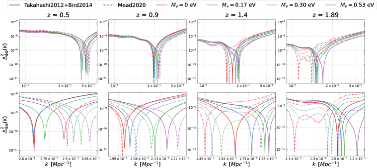
Figure 1: Top: Absolute values of the dimensionless and scaled form of the ISWRS–CMB-lensing potential cross-spectra as a function of the wavenumber $k$ at $z=0.5,0.9,1.4,1.89$ for the four neutrino total masses considered ($M_{\nu}=0,0.17,0.30,0.53$ eV as red, blue, green and purple lines, respectively), obtained via the Takahashi2012+Bird2014 model (solid lines) and the Mead2020 model (dotted lines). Bottom: Zoom-in of the top panels on the sign inversion regions.

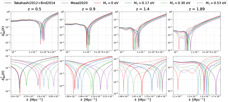
Figure 2: Top: Absolute values of the dimensionless and scaled form of the ISWRS–galaxy distribution cross-spectra as a function of the wavenumber $k$ at $z=0.5,0.9,1.4,1.89$ for the four neutrino masses considered ($M_{\nu}=0,0.17,0.30,0.53$ eV as red, blue, green and purple lines, respectively), obtained via the Takahashi2012+Bird2014 model (solid lines) and the Mead2020 model (dotted lines). Bottom: Zoom-in of the top panels on the sign inversion regions.

The panels of both Figures 1-2 show how the presence of nonlinearities varies with time. As already mentioned, the more we travel back in time, the more the RS effect will dominate over the late ISW. Considering that at large redshifts the RS traces not only nonlinearities at small scales, but even the production of filamentary structures (visible at scales of few hundreds Mpc) [49], we see the shifts of the sign inversion towards smaller $k$ (i.e. larger cosmological scales) from $z=0.5$ to $z=1.89$. In the bottom panels, the zoom in of the sign inversion region highlights the effect of massive neutrinos that we expected to find: the more neutrinos are massive, the more nonlinearities (and therefore the sign inversion) appear on smaller cosmological scales. The only exception, for both $\Delta^{2}_{\dot{\Phi}\Phi}$ and $\Delta^{2}_{\dot{\Phi}\delta}$, is the trend obtained for $M_{\nu}=0.17$ eV using the Takahashi2012+Bird2014 model at $z=0.5$, where the power spectra show the sign inversion at scales slightly larger than the massless neutrino case. This effect is probably due to inaccuracies in the nonlinear modelling (see Appendix A for further details).

These results also highlight the different behaviour of the two models. At small redshifts the Takahashi2012+Bird2014 model predicts an higher level of nonlinearities than the Mead2020 model. Indeed, in the panels of Figures 1-2 corresponding to $z=0.5$, the wavenumbers $k$ where Takahashi2012+Bird2014 sign inversions occur are smaller than Mead2020 ones. However, in both Figures it is easy to notice that at $z=0.9$ and $z=1.4$ there is a switch of trend between Takahashi2012+Bird2014 and Mead2020, and at $z=1.89$ the Mead2020 model predicts an higher level of nonlinearities with respect to Takahashi2012+Bird2014.

The presence of massive neutrinos is expected to affect similarly also the angular power-spectra of both these cross-correlations, that actually depend on the redshift derivative of the matter power spectrum $P_{\delta\delta}$, and can be computed via [54]:

$$C_{\ell}^{\dot{\Phi}\Phi}=\frac{1}{2}\Big{(}\frac{3\Omega_{m}H_{0}^{2}}{2c^{2}k^{2}}\Big{)}^{2}\int_{z_{\rm min}}^{z_{\rm max}}{\rm d}z\,\frac{\chi(z_{ls})-\chi(z)}{\chi(z_{ls})\chi^{3}(z)}\Big{[}\partial_{z}\frac{P_{\delta\delta}(k,z)}{a^{2}(z)}\Big{]}\,,$$ (2.5)

where $z_{ls}=1100$, and [21, 53, 45]:

$$C_{\ell}^{\dot{\Phi}g}=\frac{3\Omega_{m}H_{0}^{2}}{2c^{3}(\ell+1/2)^{2}}\int_{z_{\rm min}}^{z_{\rm max}}{\rm d}z\,n(z)b(z)H(z)a(z)\Big{[}\partial_{z}\frac{P_{\delta\delta}(k,z)}{a^{2}(z)}\Big{]}\,,$$ (2.6)

where $n(z)$ and $b(z)$ are the galaxy selection function and the galaxy bias, respectively. The integral limits used in this work are: $z_{\rm min}=0.02$ and $z_{\rm max}=1.89$. This is because we use Equations (2.5) and (2.6) to compute the theoretical predictions that are compared against the cross-spectra measured from the DEMNUni maps, that cover the redshift range $[0.02,1.89]$ (see Section 3). Apart from $n(z)$ and $b(z)$, all the ingredients of Equations (2.5) and (2.6) have been obtained via CAMB.

3 Nonlinear modelling with N-body simulations

The choice to investigate the nonlinear regime requires the use of large N-body simulations for validation tests. For this work, we use the “Dark Energy and Massive Neutrino Universe” (DEMNUni) [25] N-body cosmological simulations to model at small scales the ISWRS signal and their cross-correlations with the CMB-lensing and the galaxy distributions.

3.1 The Dark Energy and Massive Neutrino Universe simulations

The DEMNUni simulations have been produced with the aim of investigating large-scale structures in the presence of massive neutrinos and dynamical dark energy (DDE), and they were conceived for the nonlinear analysis and modelling of different probes, including dark matter, halo, and galaxy clustering [55, 56, 57, 58, 59, 60, 61, 62, 63, 64, 65], weak lensing, CMB-lensing, SZ and late ISW effects [66, 25, 67, 68], cosmic void statistics [69, 70, 71, 72, 73], and cross-correlations among these probes [74]. To this end, they combine a good mass resolution with a large volume to include perturbations both at large and small scales. In fact, these simulations follow the evolution of 2048³ cold dark matter (CDM) and, when present, 2048³ neutrino particles in a box of side $L=2\,h^{-1}{\rm Gpc}$. The fundamental frequency of the comoving particle snapshot is, therefore, $k_{\rm F}\approx 3\times 10^{-3}\ h/$Mpc, while the chosen softening length is 20 kpc/$h$. The simulations are initialised at $z_{\rm ini}=99$ with Zel’dovich initial conditions. The initial power spectrum is rescaled to the initial redshift via the rescaling method developed in Ref. [75]. Initial conditions are then generated with a modified version of the N-GenIC software, assuming Rayleigh random amplitudes and uniform random phases. The DEMNUni simulations have been performed using the tree particle mesh-smoothed particle hydrodynamics (TreePM-SPH) code GADGET-3, an improved version of the code described in [76], specifically modified in [77] to account for the presence of massive neutrinos. This version of GADGET-3 follows the evolution of CDM and neutrino particles, treating them as two distinct collisionless fluids. Given the large amount of memory required by the simulations, baryon physics is not included. This choice, however, does not affect the results of this work [30]. The DEMNUni suite is composed by a total of sixteen simulations accounting for different combinations of the total neutrino mass $M_{\nu}$ and the DE EoS. In this project, we have worked with four of them, characterised by a baseline Planck 2013 cosmology [5], namely a flat $\Lambda$CDM model with $\tau=0.0925$, $n_{s}=0.96$ and $A_{s}=2.13\times 10^{-9}$, generalised to a $\nu\Lambda$CDM by varying only the sum of the neutrino masses over the values $M_{\nu}=0,0.17,0.30,0.53\text{ eV}$ (whence the corresponding values of $\Omega_{\nu}$ and $\Omega_{cdm}$, keeping fixed $\Omega_{m}$ = 0.32 and $\Omega_{b}$ = 0.05), considering a degenerate neutrino mass hierarchy. As aforementioned, in this work we use maps that cover a range of redshift that goes from $z_{\rm min}=0.02$ to $z_{\rm max}=1.89$. For each simulation, 63 outputs have been produced, logarithmically equispaced in the scale factor $a=1/(1+z)$, in the redshift interval $z=0-99$, 49 of which lay between $z=0$ and $z=10$. For each of the 63 output times, it has been produced on-the-fly one particle snapshot, composed of both CDM and neutrino particles, one 3D grid of the gravitational potential, $\Phi$, and one 3D grid of its time derivative, $\dot{\Phi}$, with a mesh of dimension $4096^{3}$ that covers a comoving volume of $(2\,h^{-1}{\rm Gpc})^{3}$.

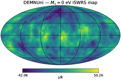
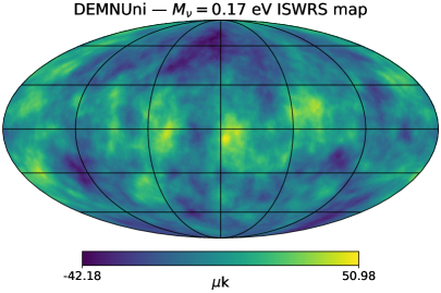
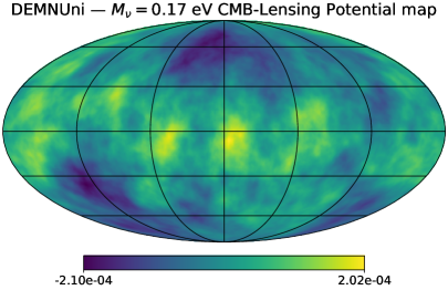
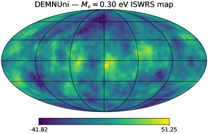
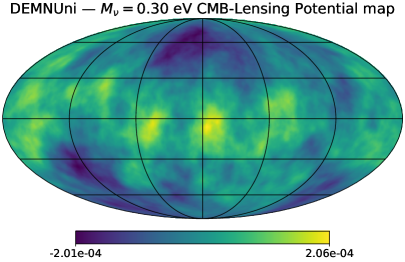
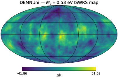
Figure 3: Full-sky maps of ISWRS (left column) and CMB-lensing potential (right column) obtained from the DEMNUni simulations for the four cosmologies used in this work: $\Lambda$CDM and $\nu\Lambda$CDM with $M_{\nu}=0.17,0.30,0.53\text{ eV}$ (from top to bottom). These maps have a pixel number and resolution given by $N_{\rm side}=2048$ and a RING ordering, following the procedure described in Section 3.2.

The map-making procedure has been developed taking into account the standard pixelisation approach introduced by the Hierarchical Equal-Area isoLatitude Pixelization [78] (HEALPix).

3.2 Map-making procedure: ISWRS and CMB-lensing

The procedure followed to build ISWRS and CMB-lensing potential maps is an adaptation of the one developed in [79]. To make ISWRS maps (left column of Figure 3), CMB photons are ray-traced along the undeflected line of sight through the 3D field $\dot{\Phi}$. An analogous kind of ray-tracing has been applied to the 3D $\Phi$-grids as well, in order to produce CMB-lensing potential maps (right column of Figure 3) from the same realisation of the Universe as for the ISWRS maps, and compute the cross-correlation between the two maps. Comparing the left and right columns of Figure 3, it is possible to appreciate at a glance how the two signals are highly correlated. Comparing the scales of each rows, the slight difference due to the different $M_{\nu}$ considered emerges. To this aim, the $\dot{\Phi}$- and $\Phi$-grids have been stacked around the observer, located at $z=0$, and it has been applied the replication and randomisation procedure designed by [79]. This particular 3D tessellation scheme is required to avoid both the repetition of the same structures along the line of sight and the generation of artifacts like ripples in the simulated deflection-angle field, which can be avoided only if the peculiar gravitational potential is continuous transversely to each line of sight.

3.2.1 Simulated ISWRS and CMB-lensing auto-spectra

The power spectra extracted from the maps of Figure 3 are reported in Figure 4. For comparison, the orange squares and the orange dashed lines represent theoretical predictions in the linear regime obtained with CAMB for the massless neutrino case, in order to highlight the differences from the nonlinear modelling. The subpanels represent the percentage relative differences of the $\nu\Lambda$CDM models with respect to the massless neutrino one. There is a good agreement between the simulated ISWRS signals and the ones predicted with CAMB for $\ell<100$ (which roughly corresponds to the transition between the linear and the nonlinear regimes [80, 81]). Past the linear limit, CAMB predictions fail, given that the RS contribution is not implemented in the code. The CMB-lensing potential linear prediction for the massless neutrino case, similarly, perfectly agrees with DEMNUni mocks up to the linear limit and then shows a lack of power with respect to the nonlinear ones.

Focusing on spectra extracted from maps, it is easy to appreciate at small scales the differences produced in the ISWRS induced temperature anisotropies by free-streaming neutrinos with different total masses. Similar effects are noticeable also in the lensing potential power spectra, considering the percentage relative differences with respect to the massless neutrino case (see subpanels of Figure 4). In particular, as expected, the effect of massive neutrinos produces a suppression of power in the CMB-lensing potential which increases with the neutrino mass and decreases with the angular scale (at low $\ell$). This effect is reasonably due to the nonlinear excess of suppression of the total matter power spectra with respect to linear expectations in the presence of massive neutrinos, that counteract the nonlinear evolution [25].

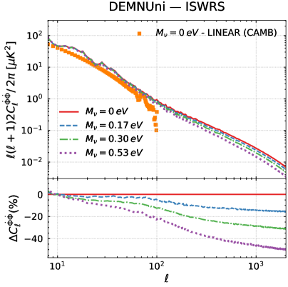
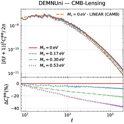
Figure 4: Left: Angular power spectra of the total ISWRS induced temperature anisotropies computed from DEMNUni maps with $M_{\nu}=0,0.17,0.30,0.53\text{ eV}$ (solid red, dashed blue, dot-dashed green, dotted purple lines, respectively) compared with linear prediction (orange squares). Right: Same for angular power spectra of the CMB-lensing. In both subpanels, the percentage relative differences with respect to the massless neutrino case is reported.

3.3 Map-making procedure: projected galaxy mocks

The procedure followed to construct galaxy maps is an adaptation of the one developed in [82, 67] for convergence maps. The convergence maps are extracted with a postprocessing procedure acting on the N-body particle snapshots to create matter particle full-sky lightcones [83, 84]. The standard way to build lightcones is to pile up high-resolution boxes within concentric cells to fill the lightcone to the maximum desired source redshift. With the observer placed at $z=0$, the volume of the lightcone is sliced into full-sky spherical shells of the desired thickness in redshift. All the particles distributed within each of these 3D matter shells are

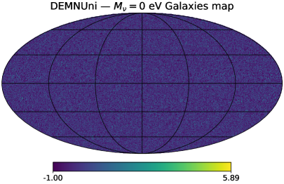
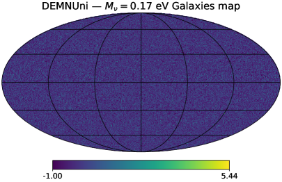
Figure 5: Full-sky galaxies maps obtained for the four cosmologies used in this work: $\Lambda$CDM and $\nu\Lambda$CDM with $M_{\nu}=0.17,0.30,0.53\text{ eV}$. These maps have a pixel number and resolution given by $N_{\rm side}=2048$ and a RING ordering, following the procedure described in Section 3.3.

then projected onto 2D spherical maps, assigning a specific sky pixel to each particle, via HEALPix pixelisation procedure. Then integration along the undeflected line-of-sight is applied to obtain the convergence maps accounting for the lensing efficiency in the desired redshift range. A very similar method has been applied to the DEMNUni galaxies to construct projected galaxies mocks [61] (see Figure 5). Specifically, in order to reproduce the galaxy distribution in the DEMNUni simulations, the SubHalo Abundance Matching (SHAM) technique [65] has been used. The SHAM method assumes a one-to-one relation between a physical property of a dark matter halo/subhalo and an observational property of the galaxy that it hosts. In particular, it assumes that the most massive galaxies form in the dark matter haloes characterised by the deepest potential wells. Galaxies are linked to the corresponding dark matter structures using stellar mass or luminosity as galaxy property and a measure of halo mass or the circular velocity, as halo property (i.e. a proxy of the depth of the local potential well). Here we link the stellar mass to the halo mass using the Moster et al. (2010) [85] parameterised stellar-to-halo mass relation, fitted against the DEMNUni simulations. As the SHAM galaxy catalogues are fitted against observations, they guarantee an high-degree of agreement with real data from galaxy surveys [86, 87].

Applying to the SHAM galaxy catalogues the same stacking technique as for particle comoving snapshots, we have generated full-sky mock galaxy catalogues from the DEMNUni simulations in different cosmological models.

3.3.1 Galaxy bias and selection function from DEMNUni simulations

The galaxy bias and selection function necessary to compute the analytical predictions of the cross-spectra between ISWRS and galaxies (see Equation (2.6)) have been directly extracted from the DEMNUni simulations. This guarantees a more accurate comparison between mocks and analytical predictions.

Galaxy selection function

The galaxy selection function extracted from DEMNUni $\Lambda$CDM map can be modelled via the following equation:

$$n_{\rm DEMNUni}(z)=A\left(\frac{z}{z_{0}}\right)^{B}\exp\Big{[}-\Big{(}\frac{z}{z_{0}}\Big{)}^{C}\Big{]}\,,$$ (3.1)

where A = 1.89, B = 1.95, C = 1.41 and $z_{0}=0.88$.

This is the $n(z)$ used to compute all the theoretical predictions to be compared with DEMNUni data, also for massive neutrino cases. This is because galaxy counts vary mostly because of the variation of the simulated cosmological volume, which depends on $H(z)$ via $\Omega_{m}$ - that has been fixed to 0.32 for all the simulations (and consequently for all the theoretical predictions) - and via the DE EoS, whose presence has not been taken into account in this work. As a result, the normalised galaxy counts do not undergo any significant change due to the variation of $M_{\nu}$, and consequently it is possible to exploit the same $n(z)$ to compute all the theoretical predictions. We have verified this measuring the galaxy counts from the DEMNUni catalogues with different values of $M_{\nu}$, obtained via the SHAM technique applied to COSMOS2020 and SDSS observations  [65].

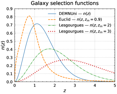
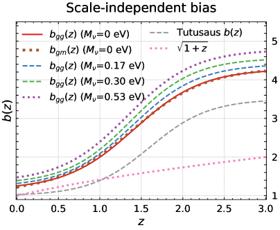
Figure 6: Left: Galaxy selection functions: the solid blue line is extracted from DEMNUni data; the dashed orange line is the one assumed for the photometric Euclid survey; the dot-dashed green and the dotted red lines are taken from Lesgourgues et al. (2008) [21] with $z_{m}=2,3$ respectively. Right: Scale-independent galaxy bias: the solid red, dashed blue, dot-dashed green and dotted purple lines are the $b_{gg}(z)$ extracted from the DEMNUni simulations for $M_{\nu}=0,0.17,0.30,0.53$ eV, respectively; the dotted brown line is the $b_{gm}(z)$ extracted from the DEMNUni simulations for the massless neutrino case only; the dashed grey line is the Tutusaus bias [88]and the dotted pink line is the $\sqrt{1+z}$ bias.

In Figure 6, together with DEMNUni $n(z)$, we show the galaxy selection function expected for the photometric Euclid survey [33, 34]:

$$n_{\rm Euclid}(z)=\frac{3\cdot(z/z_{0})^{\alpha}}{2\cdot z_{0}}\text{exp}\Big{[}-\Big{(}\frac{z}{z_{0}}\Big{)}^{\beta}\Big{]}\,,$$ (3.2)

where $\alpha$ = 2, $\beta$ = 1.5, $z_{0}$ = $z_{m}/\sqrt{2}$, $z_{m}$ = 0.9, and its extensions to a larger redshift range setting $z_{m}$ = 2,3 [21]. These functions have been used here to produce forecasts for future galaxy surveys, whose aim is to reach $z\geq 2$.

Scale-independent bias

The galaxy scale-independent bias has been obtained for each cosmology from the square root of the ratio between the galaxy power spectrum, $P_{gg}(k,z)$, and the matter power spectrum, $P_{mm}(k,z)$, measured from DEMNUni comoving snaphots:

$$b_{gg}(z)=\Bigg{\langle}\sqrt{\frac{P_{gg}(k,z)}{P_{mm}(k,z)}}\Bigg{\rangle}_{k}\,,$$ (3.3)

where the mean has been computed for large linear scales in the range $0.05<k<0.12$ in unit of $\text{Mpc}^{-}1$. Differently from the galaxy selection function, the neutrino mass affects the bias. The $b_{gg}$ functions for $M_{\nu}=0,0.17,0.30,0.53$ eV shown in the right panel of Figure 6 have been fitted with:

$$b(z)=A+\frac{B}{1+\exp[-(z-D){C}]}\,,$$ (3.4)

where A = 1.0, B = 2.5, C = 2.8, D = 1.6. This is the bias currently assumed for the Euclid Flagship simulation, reported in [88]. From now on, we will refer to Equation (3.4) as the Tutusaus bias.

For the massless neutrino case alone, also the bias obtained from the square root of the ratio between the cross power spectrum between galaxy and matter has been computed:

$$b_{gm}(z)=\Bigg{\langle}\sqrt{\frac{P_{gm}(k,z)}{P_{mm}(k,z)}}\Bigg{\rangle}_{k}\,,$$ (3.5)

(where the mean is again over large linear scales in the range $0.05<k<0.12$ in unit of $\text{Mpc}^{-}1$) and it is shown in Figure 6 after the fit with Tutusaus bias. Since it is affected by a lower level of shot noise, $b_{gm}(z)$ should allow us to describe better the connection between matter and galaxies, and consequently to improve the cross-correlation reconstruction. However, the results obtained do not differ significantly from those obtained using $b_{gg}(z)$, as we will show in Section 5.1.2. Finally, we show also the $\sqrt{1+z}$ bias, used in [34].

Scale-dependent bias

A fit of scale-dependent bias has been computed from DEMNUni massless neutrino mocks as [89]:

$$b(k,z)=b_{0}(z)+b_{1}(z)k+b_{2}(z)k^{2}\,,$$ (3.6)

where $b_{0}$ is the scale-independent bias, $b_{2}$ is a correction due to peaks theory and $b_{1}$ is physically meaningless, but necessary to improve the fit. These parameters have been obtained via the fit of $P_{gg}(k,z)$ up to $k=1\text{ Mpc}^{-1}$. In Figure 7, we show the evolution of the $b_{i}$ parameters on the left, while on the right we show the variation of the $b(k,z)$ at some chosen wavenumbers in the range of scales used to measure the scale-averaged the $b_{gg}(z)$ ($0.05<k<0.12$ in unit of $\text{Mpc}^{-}1$).

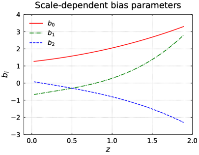
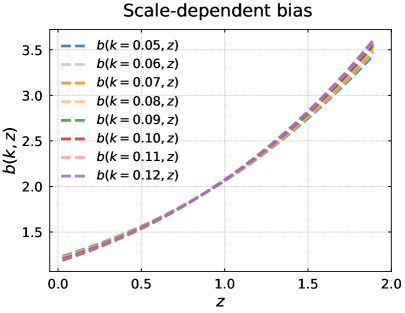
Figure 7: Left: Evolution of $b_{i}(z)$ parameters from Equation (3.6) in the DEMNUni maps redshift range $0.02\leq z\leq 1.89$. Right: Scale-dependent bias computed for large scales in the range $0.05<k<0.12$.

3.3.2 Simulated projected galaxy auto-spectra

In Figure 8, we report the spectra extracted from the galaxy maps of Figure 5 after subtracting the shot-noise value.

In addition to the DEMNUni maps spectra, we report the theoretical predictions of the $C_{\ell}^{gg}$ computed in both the linear and nonlinear regimes, for the massless neutrino case, via [90]:

$$C_{\ell}^{gg}=\int_{z_{\rm min}}^{z_{\rm max}}{\rm d}z\,\frac{H(z)}{c\chi^{2}(z)}[W^{g}(z)]^{2}P_{\delta\delta}(k,z)\,,$$ (3.7)

where:

$$W^{g}(z)=n(z)\cdot b(z)\,,$$ (3.8)

and for $n(z)$ and $b(z)$ we use Equation (3.1) and Equation (3.3), respectively.

Both linear and nonlinear predictions do not perfectly agree with simulated spectra on large scales. This is due to the limited dimension of the simulation box, which does not allow to represent those scales. Conversely, on small scales there is a good agreement with the nonlinear prediction and the expected disagreement with the linear one.

Despite the presence of shot-noise in DEMNUni maps, its effect is negligible when cross-correlating these maps with ISWRS maps (since the noises of the two fields do not correlate). Furthermore, this analysis does not aim to reveal a perfect match between the simulations and the analytical predictions also because inaccuracies in the adopted nonlinear modelling.

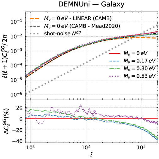
Figure 8: Galaxy angular auto-spectra extracted from DEMNUni maps for $M_{\nu}=0,0.17,0.30,0.53$ eV (solid red, dashed blue, dot-dashed green, dotted purple lines, respectively) with shot-noise (dotted grey line) subtracted, compared with theoretical predictions in the linear (dashed orange line) and Mead2020 nonlinear (dashed black line) regimes. In the subpanel, the percentage relative difference with respect to the massless neutrino case is reported.

The subpanel in Figure 8 represents the percentage relative differences of the $\nu\Lambda$CDM models with respect to the massless neutrino one. Here the larger $M_{\nu}$ is, the smaller the difference with respect to the massless neutrino case is. This is because the matter perturbation suppression due to more massive neutrinos is compensated by a stronger clustering [91].

4 The ISWRS cross-correlation with the CMB-lensing potential

The presence of the sign inversion at large multipoles and its shift due to the variation of $M_{\nu}$ in the cross-power spectrum between the ISWRS effect and the CMB-lensing was already verified in [25], where they use DEMNUni maps obtained via ray-tracing from $z_{\rm min}=0.02$ to $z_{\rm max}=20.88$. Here, we verify the presence of the same effects in the cross-spectra of DEMNUni maps obtained up to $z_{\rm max}=1.89$ and use these results to validate the analytical predictions computed using Equation (2.5).
The cross-correlations of the DEMNUni ISWRS and CMB-lensing potential maps for the four neutrino masses are shown in Figure 9, compared with the theoretical nonlinear prediction computed for the Takahashi2012+Bird2014 (left panels) and the Mead2020 (right panels) models. For completeness, also the theoretical cross-correlation predictions for the massless neutrino case in the linear regime have been reported.

The agreement between the simulation data and both the theoretical predictions obtained with CAMB up to $\ell\sim 100$ is quite impressive. Once exceeded $\ell\sim 100$, the anti-correlation between the RS effect and the CMB-lensing potential takes over, resulting in the characteristic sign inversion that appears in both simulations (as already shown in [25]) and nonlinear predictions. Moreover, both of them validate the expected result, because the more neutrinos are massive, the more they counteract nonlinear evolution (i.e. structure formation) and nonlinear effects appear at smaller cosmological scales. In other words, the more neutrinos are massive, the more the sign inversion shifts towards larger multipoles.

Focusing on the sign inversion position (subpanels), on the one hand the analytical predictions computed with the Mead2020 model show the sign inversions at smaller multipoles with respect to mocks and with respect to the Takahashi2012+Bird2014 model. On the other hand, the Takahashi2012+Bird2014 model almost perfectly reproduces the results of DEMNUni mocks for $M_{\nu}=0.17,0.30$ eV, while overestimating the $\ell$ correspondent to the sign inversion in the massless neutrino case and underestimating it in the more massive case. The differences between the two nonlinear models are strictly due to how nonlinearities are implemented in the two codes [29, 30, 31, 61]. The achieved results disprove the counter-intuitive effect reported in [92], where for larger $M_{\nu}$ values the sign inversion position moves towards smaller multipoles.

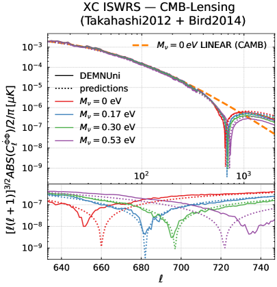
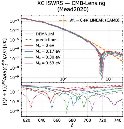
Figure 9: ISWRS – CMB-lensing angular cross-spectra for $M_{\nu}=0,0.17,0.30,0.53\text{ eV}$ (solid red, blue, green and purple lines, respectively) from the DEMNUni maps compared to the theoretical predictions in the linear (dashed orange line) and nonlinear (dotted lines) regimes, obtained using the Takahashi2012+Bird2014 model (left) and the Mead2020 model (right), respectively. The subpanels show a zoom-in of the top panels on the sign inversion regions.

5 The ISWRS cross-correlation with galaxies

The cross-spectra between the ISWRS signal and the galaxy distribution is the most used tool to investigate the ISWRS, because of its largest signal-to-noise ratio with respect to the spectra analysed in the previous Section. It is then the main focus of this work, which consists of verifying the presence of the sign inversion due to the anti-correlation between the RS effect and the galaxy distribution in the cross-correlation angular power spectra, showing that the position of this sign inversion depends on $M_{\nu}$, as in the case of the cross-correlation between the ISWRS signal and the CMB-lensing potential [25]. The validation of these results via DEMNUni maps represents an improvement with respect to previous works: on the one hand, [21] computed this cross-correlation signal in massless and massive neutrino models, focusing only on the effects that neutrinos have in the linear regime; on the other hand, in the nonlinear regime, [53] focused only on the massless neutrino case, finding in the cross-spectrum the sign inversion due to the anti-correlation between the RS effect and the galaxy distribution.

The cross-correlations of the DEMNUni ISWRS and the galaxy distribution maps for the four neutrino masses are shown in Figure 10, compared with the theoretical nonlinear predictions, computed with Equation (2.6). For completeness, also the theoretical predictions for the massless neutrino case in the linear regime have been reported. All the theoretical predictions have been computed using $n(z)$ given by Equation (3.1) and the $b_{gg}(z)$ of Equation (3.3) associated with the cosmology analysed.

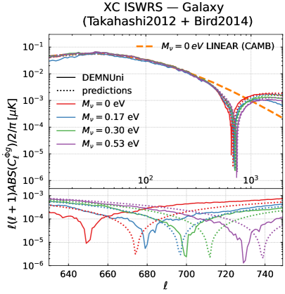
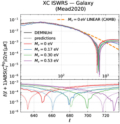
Figure 10: ISWRS-galaxy cross-spectra for $M_{\nu}=0,0.17,0.30,0.53\text{ eV}$ (solid red, blue, green and purple lines, respectively) compared with theoretical predictions in the linear (dashed orange line) and nonlinear (dotted lines) regimes, obtained using the Takahashi2012+Bird2014 model (left) and the Mead2020 model (right), respectively. The subpanels show a zoom-in of the top panels on the sign inversion regions.

The results shown prove that also in the cross-correlation spectrum between the ISWRS and the galaxy distribution there is a sign inversion due to the anti-correlation between the two signals on small scales and that the position of the sign inversion is strongly affected by the presence of massive neutrinos. Also in this case, because of the suppression that massive neutrinos induce in the matter power spectrum, the larger $M_{\nu}$ is, the more nonlinearities appear on smaller scales and consequently the sign inversion position is shifted towards larger multipoles.

Moreover, the comparison of the simulated spectra with the theoretical predictions for both linear and nonlinear regimes is again quite impressive at large cosmological scales, while once passed $\ell\simeq 100$ nonlinear spectra dramatically differ from the linear one, because of the presence of the sign inversion. This result validates again the analytical method against mocks and makes it an extremely powerful tool to predict cross-spectra of future surveys in both linear and nonlinear regimes.

Focusing on the sign inversion position (subpanels), the Takahashi2012+Bird2014 model shows inversions at larger multipoles with respect to DEMNUni spectra, and Mead2020 at smaller ones.

5.1 Nonlinear ISWRS-galaxy cross-spectra: effects of different bias modellings

As already mentioned, differently from the galaxy selection function, the bias strongly depends on the neutrino mass. We perform several tests to evaluate how the usage of different bias functions affects the comparison between predictions and DEMNUni simulations. First, we produce theoretical predictions for the massive neutrino cases using both the corresponding bias and the massless neutrino bias functions and we verify that the more neutrinos are massive, the more the massless neutrino case bias fails in predicting the spectra (further details in Section 5.1.1). Second, we check, for the massless neutrino case alone, that using a scale-dependent bias function improves the agreement between theoretical predictions and simulations, as already verified in [53] (further details in Section 5.1.2). The results of these tests are shown in Figure 11 and Figure 12, respectively.

5.1.1 Massive neutrino impact on the scale-independent bias

First, we test how the analytical predictions for massive neutrino cosmologies vary with respect to mock data when using the bias fitted against the simulations for the $M_{\nu}>0\text{ eV}$ case and the bias of the massless neutrino case.

In Figure 11, the simulated cross-correlations are compared with linear predictions and with nonlinear predictions computed with both the massless neutrino galaxy bias and the galaxy bias associated with the specific neutrino model. The results for $\ell\leq 10$ can be neglected because of the inaccuracies of mocks on those scales.

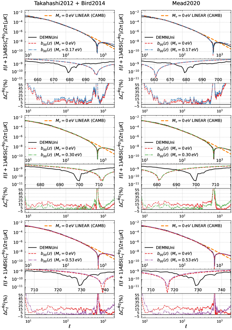
Figure 11: Left: Comparison between the simulated ISWRS-galaxy cross-correlations for $M_{\nu}=0.17,0.30,0.53$ eV (solid black line) and theoretical predictions in the linear (dashed orange line) and nonlinear regimes, using the Takahashi2012+Bird2014 model combined with DEMNUni measurements of $b_{gg}$ in the massless neutrino (dashed red) and massive neutrino cases for $M_{\nu}=0.17\text{ eV}$ (top, dot-dashed blue), $M_{\nu}=0.30\text{ eV}$ (middle, dot-dashed green) and $M_{\nu}=0.53\text{ eV}$ (bottom, dot-dashed purple), respectively. The middle subpanel of each plot shows a zoom-in of the sign inversion region, while the bottom one shows the absolute value of the percentage relative differences of the predictions with respect to the simulated measurements. Right: Same as the left panel for the Mead2020 model.

For the $M_{\nu}=0.17\text{ eV}$ case, reported in top panels of Figure 11, the slight difference with respect to the other cases (and to the predictions), noticeable in the simulation data for very small and very large multipoles, induces a difference $>35\%$ for $\ell<30$ and $\ell>1000$. Before the sign inversion range, the differences do not overcome $25\%$ for the $M_{\nu}=0.17$ eV bias and $15\%$ for the massless neutrino case bias, for the Takahashi2012+Bird2014 modelling. In the case of the Mead2020 modelling, the difference is slightly smaller with the massive cosmology bias ($<20\%$). The differences in the sign inversion positions consist of $\Delta\ell_{\rm DEMNUni-(Takahashi2012+Bird2014)}\sim-18$ and $\Delta\ell_{\rm DEMNUni-Mead}\sim+18$. Both nonlinear modellings show a difference between the predictions obtained with the two bias recipes at a level of $\sim 5\%$ and the sign inversions occur at the same multipole in the Mead2020 model, while there is a $\Delta\ell=1$ for the Takahashi2012+Bird2014 one. The fact that the massless neutrino cosmology bias in the theoretical predictions leads to smaller differences with respect to the DEMNUni spectra can be explained considering the inaccuracies of the Takahashi2012+Bird2014 and Mead2020 models in reproducing the $M_{\nu}=0.17$ eV case, as already shown in Section 2 (see Appendix A for further details).

In the $M_{\nu}=0.30\text{ eV}$ case, shown in centre panels of Figure 11, both nonlinear predictions, obtained with the Mead2020 and Takahashi2012+Bird2014 models, differ from the simulated data by no more than $15\%$ in the $M_{\nu}=30$ eV bias case and no more than $25\%$ in the massless neutrino case. The differences in the sign inversion positions consist of $\Delta\ell_{\rm DEMNUni-(Takahashi2012+Bird2014)}\sim-10$ and $\Delta\ell_{\rm DEMNUni-Mead}\sim+20$. The difference between the two is larger than the previous case ($\raisebox{-3.69899pt}{~{}\shortstack{$<$ \\ [-0.07cm] $\sim$}}~{}10\%$) and the sign inversions occur at the same multipole in the Mead2020 model, while there is a $\Delta\ell=1$ for the Takahashi2012+Bird2014 one.

Conversely to the previous cases, in the $M_{\nu}=0.53\text{ eV}$ one, shown in bottom panels of Figure 11, the difference between the predictions is definitely more significant ($\sim 20\%$). The difference with respect to DEMNUni data is $\sim 10\%$ in the $M_{\nu}=0.53$ eV bias case and no more than $25\%$ in the massless neutrino case. The differences in the sign inversion positions consist of $\Delta\ell_{\rm DEMNUni-(Takahashi2012+Bird2014)}\sim-10$ and $\Delta\ell_{\rm DEMNUni-Mead}\sim+10$. Conversely to previous cases, here the sign inversions occur in the same multipole when using both Halofit models.

5.1.2 Scale-independent and scale-dependent bias effects in the neutrino massless neutrino case

For the massless neutrino case, both the $b_{mg}(z)$ and the $b(k,z)$ bias functions have been calibrated against the DEMNUni simulations. In Figure 12 we compare the effects of $b_{mg}(z)$, $b(k,z)$ and $b_{gg}(z)$ in the modelling of the theoretical nonlinear predictions. In agreement with the work of [53], we find that the amplitude of the predictions obtained with $b(k,z)$ better reproduces the simulated signals, with a percentage relative difference of $\sim 10\%$, lower than that obtained with $b_{gg}(z)$ and $b_{mg}(z)$. This is true up to $\ell=200$, while for smaller scales the trend is inverted. With regard to the sign inversion position, in the theoretical spectra it occurs at the same multipole for all bias recipes with both Takahashi2012+Bird2014 and Mead2020 model. The differences with respect to the sign inversion in the simulated signals is $\Delta\ell_{\rm DEMNUni-(Takahashi2012+Bird2014)}\sim-20$ and $\Delta\ell_{\rm DEMNUni-Mead}\sim+20$.

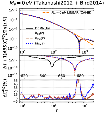
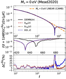
Figure 12: Left: Comparison between the simulated ISWRS-galaxy cross-correlation for $M_{\nu}=0\text{ eV}$ (solid black line) with theoretical predictions in the linear regime (dashed orange line) and nonlinear regime using the Takahashi2012+Bird2014 model. Three different DEMNUni galaxy bias models have been tested: the scale-independent DEMNUni – $b_{gg}$ bias (dashed red), the scale-independent DEMNUni – $b_{mg}$ bias (dot-dashed brow) and the scale-dependent DEMNUni $b(k,z)$ bias (dotted blue). The middle subpanel of the plot shows a zoom in of the sign inversion region, while the bottom one shows the absolute value of the percentage relative differences of the predictions with respect to the simulations. Right: Same as left, but with the Mead2020 model.

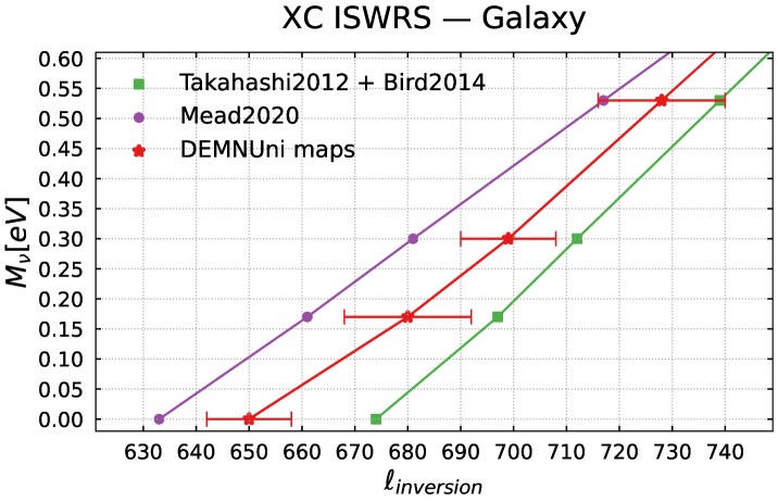
Figure 13: $M_{\nu}$ as a function of $\ell_{inv}$. The green squares represent the result of $\ell_{inv}$ from Takahashi2012+Bird2014 model predictions with different cosmological scenarios, while the purple points are taken from Mead2020 model predictions. The red stars are the results of DEMNUni simulations. The error bars are estimated from Gaussian mocks.

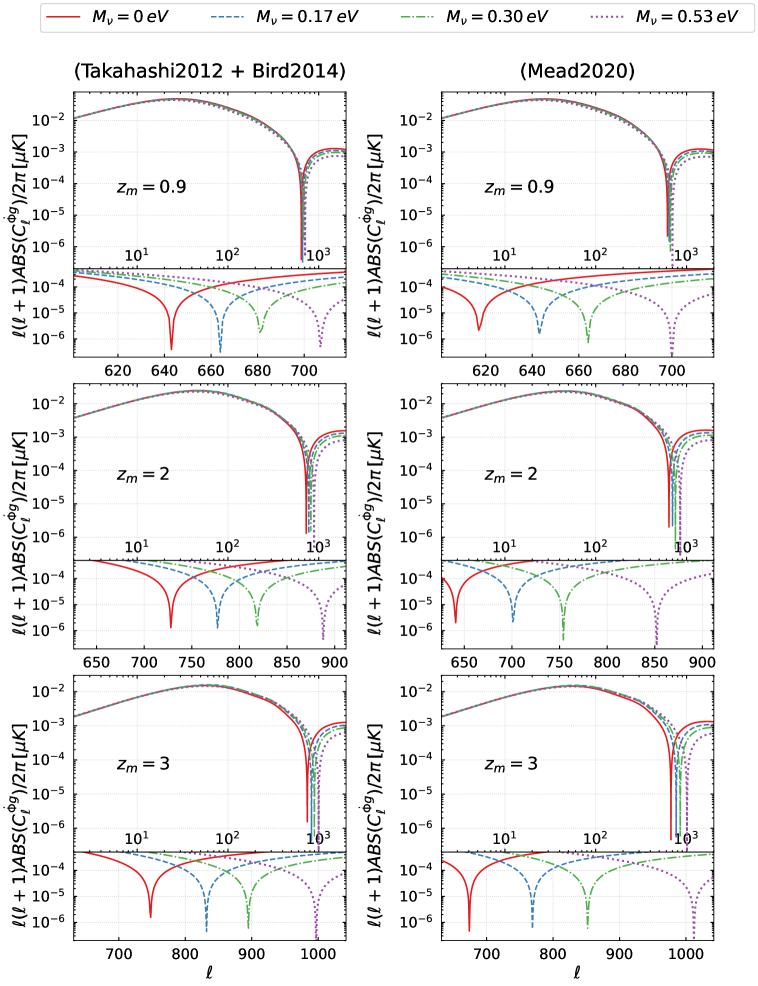
Figure 14: Left: Predictions of the ISWRS-galaxy cross-spectra for $M_{\nu}=0,0.17,0.30,0.53$ eV (solid red, dashed blue, dot-dashed green and dotted purple lines, respectively), computed with the Takahashi2012+Bird2014 model using: $n_{z}$ from Equation (3.2) with $z_{m}$ = 0.9 (top panel), which corresponds to the Euclid photometric survey, $z_{m}$ = 2 (centre panel) and $z_{m}$ = 3 (bottom panel). The subpanels of each plot show a zoom in of the sign inversion region. Right: Same as the left panels for the Mead2020 model.

5.2 Nonlinear ISWRS-galaxy cross-spectra: detecting the neutrino mass

The results shown in the previous sections demonstrate the validity of the analytical method against DEMNUni simulations and that both mocks and predictions confirm what we expect from theory: more massive neutrinos induce a larger suppression in the matter power spectrum and shift the appearance of nonlinearities on smaller cosmological scales. Moreover, Figures 9 and 10 highlight the strict connection between the sign inversion position, $\ell_{inv}$, and $M_{\nu}$. In light of this, we decide to test if the detection of $\ell_{inv}$ in the cross-power spectrum between the ISWRS and the galaxy distribution computed with Equation (2.6) can constrain $M_{\nu}$.

In Figure 13 we report the neutrino masses as a function of the sign inversion positions predicted by the Takahashi2012+Bird2014 and Mead2020 models and the DEMNUni maps. The $1\sigma$ error bars have been estimated as follows: we generate 5000 Gaussian realisations of the DEMNUni maps and estimate the errors as the standard deviation of the 5000 cross-spectra obtained from them.

For relevant values of the neutrino mass ($M_{\nu}<0.12$ eV at $95\%$ C.L. [7]), we find differences between the Takahashi2012+Bird2014 and Mead2020 models and the DEMNUni simulations at the $\sim 1.5-2\sigma$ level. This implies that robust constraints on the neutrino mass via the sign inversion detection will require improving the nonlinear modelling. Furthermore, because of cosmic variace at the multipole range of interest (see Appendix B) the possibility of detecting $\ell_{inv}$ appears to be unlikely. Nevertheless, we expect to be able to disentangle different $M_{\nu}$ values via the estimation of the overall amplitude of the signal on very small cosmological scales. As shown in [45], the accuracy of future CMB surveys will improve the detection of the T-galaxy cross-spectrum on extremely large multipoles. In future works, we plan to investigate this possibility.

5.3 Nonlinear ISWRS-galaxy cross-spectra: the case of different galaxy surveys

The last part of this work consists of computing predictions of the cross-spectra that can be observed on higher redshift ranges. First of all, we compute the ISWRS-galaxy distribution cross-power spectra that should be observable in a redshift range that goes up to $z=2$, which is Euclid photometric range [35], setting $n(z)$ from Equation (3.2) with $z_{m}$ = 0.9, shown in the upper panels of Figure 14. In the middle and bottom panels we report the cross-spectra obtained using the same $n(z)$, but with $z_{m}$ = 2, 3 respectively (see Figure 6). Differently from all the previous theoretical spectra showed, here all the predictions have been computed integrating up to $z_{\rm max}=8$. It is evident at first glance that the higher is the redshift, the larger is the difference between the four $M_{\nu}$ values, with both the Halofit models considered so far. This is because the late Universe (i.e. small $z$) is characterised by the presence of DE [93], that affects the appearance of nonlinearities and is expected to have similar effects as neutrinos on this cross-spectrum. Hence, the further we go back in time, the less DE effects will be present, and the shift we measure will be due only to the mass of neutrinos.

6 Conclusions

The aim of this work is to develop and validate, against the DEMNuni cosmological simulations, an analytical modelling able to reproduce the cross-power spectra of the ISWRS signal with the CMB-lensing potential and the galaxy distribution in the presence of massive neutrinos.

We consider both the linear (ISW) and nonlinear (RS) effects, i.e. we account also for the nonlinear regime where a sign inversion appears in the cross-spectra due to the anti-correlation between the RS effect and the CMB-lensing/galaxy-distribution. We find that the presence of massive neutrinos affects the position of such a sign inversion, and specifically, the more massive neutrinos are, the more it shifts towards larger multipoles $\ell$. This is because the more massive neutrinos, the more they suppress the matter power spectrum, shifting the appearance of nonlinearities towards smaller cosmological scales.

There is already evidence of this effect at the level of the matter power spectra, $P_{\dot{\Phi}\Phi}$ and $P_{\dot{\Phi}\delta}$, associated to these cross-correlations, as we show in Section 2. We compute them assuming a Planck-like baseline cosmology to which we add neutrinos with total mass $M_{\nu}=0.17,0.30,0.53\text{ eV}$ and using two Halofit models implemented in CAMB (Takahashi2012+Bird2014 and Mead2020) that allow us to investigate also high redshifts. We verify that a sign inversion appears in the transition from the linear to the nonlinear regime and that the presence of massive neutrinos affects its position. Moreover, we find that the lower the redshift is, the larger the scale is where nonlinearities appear, because the RS effect dominates over the late ISW one, as we go back in time.

Focussing on the nonlinear modelling, we find that Takahashi2012+Bird2014 predicts an higher level of nonlinearities with respect to Mead2020 at small redshifts, but this trend is inverted at $z\geq 1.1$ (see Figures 1 and  2).

The main result of this work is checking and modelling the presence of the same effects in the corresponding angular cross-power spectra, obtained from $P_{\dot{\Phi}\Phi}$ and $P_{\dot{\Phi}\delta}$, using Equation (2.5) and Equation (2.6).

Concerning the cross-correlation between the ISWRS signal and the CMB-lensing potential, we find that both DEMNUni maps and the theoretical predictions, computed using the Takahashi2012+Bird2014 and Mead2020 models, show the sign inversion due to the anti-correlation between the RS and the CMB-lensing, and the shift of this sign inversion moves towards larger multipoles as $M_{\nu}$ increases (see Figure 9).

Furthermore, we observe that, while the modelling implementing Mead2020 tends to overestimate nonlinearities (and the sign inversions appear always on smaller multipoles with respect to the DEMNUni simulated signal), the Takahashi2012+Bird2014 modelling gives different results depending on $M_{\nu}$, and the corresponding sign inversion locations are indeed extremely close to those of the simulations for $M_{\nu}=0.17,0.30$ eV.

The same results have been achieved for the cross-correlation between the ISWRS and the galaxy distribution with both DEMNUni maps and the theoretical predictions (see Figure 10). This represents an improvement with respect to [53], where only the massless neutrino case was investigated, and extends the work of [21] properly treating the impact of massive neutrinos on this cross-correlation in the nonlinear regime. We find that the Takahashi2012+Bird2014 modelling consistently underestimates nonlinearities compared to simulations, resulting in sign inversions occurring on smaller cosmological scales, i.e. larger multipoles. Conversely, the Mead2020 modelling overestimates nonlinearities. This could be due to the fact that such models are not correctly able to recover the time variation of the gravitational potentials which give rise to the ISWRS effect.

Considering the dependence of this cross-correlation on galaxy bias, we have performed two further tests to quantify the effects of different bias modellings. First, we test how the analytical predictions fit the simulated signal when considering a bias (measured from the DEMNUni simulations) dependent or not on the neutrino mass. We observe that, for small values of $M_{\nu}$, the differences between the modelling with massless and massive neutrino bias are negligible (Figure 11). Conversely, when considering large values of $M_{\nu}$, the difference cannot be neglected, and a bias model specific to that cosmology is required. However, in view of the fact that the most recent constraints on neutrino masses suggest $M_{\nu}<0.12$ eV [7], a bias associated to a massless neutrino case cosmology would be appropriate to produce accurate forecasts, at least in a $\Lambda$CDM scenario. Second, only in the massless neutrino case, we test the effect of scale-independent and scale-dependent bias as measured from the DEMNUni. We verify that, both for Takahashi2012+Bird2014 and Mead modellings, choosing a scale-dependent bias $b(k,z)$ results in spectra whose amplitudes better fit the simulated signal (Figure 12), as suggested in [53].

Overall in this work, we have developed an analytical modelling of the nonlinear ISWRS-LSS cross-correlations that exploits the Boltzmann solver code CAMB and has been validated against the DEMNUni simulations [25]. It is a useful and computationally non-expensive tool to investigate these cross-correlations in different cosmological scenarios without the need to run large N-body simulations for each cosmology.

We have verified that these cross-spectra change with redshift because of the different role played by dark energy at different epochs. Therefore, a straightforward extension of this work would be to include DDE models in the analysis, and study the dependency on the DE equation of state of the ISWRS-LSS cross-spectra. This could help to distinguish between different DE models and provide insights on the properties and the evolution of DE.

Finally, our results highlight the strict connection between the sign inversion location, $\ell_{inv}$, and the value of neutrino masses. However, improving current nonlinear modellings of the matter power spectra is needed to predict $\ell_{inv}$ accurately. In a future work we will investigate the detectability of the neutrino mass via ISWRS-LSS cross-correlations. We expect future CMB experiments, such as The Simons Observatory [94], LiteBIRD[95], CMB-S4 [43], and galaxy surveys such as Euclid [35], the Roman Space telescope [96], the Vera Rubin Observatory [97], will help us exploiting such nonlinear signals with the aim of measuring, in combination with more traditional probes, the neutrino mass and the DE equation of state.

Appendix A Test nonlinearities in the dark matter power spectra

As showed in Section 2 (Figure 1 and Figure 2), there are inaccuracies in the Takahashi2012+Bird2014 nonlinear model in the representation of both $P_{\dot{\Phi}\Phi}$ and $P_{\dot{\Phi}\delta}$ at $z=0.5$, where the sign inversion for the $M_{\nu}=0.17$ eV case occurs at larger multipoles than the massless neutrino one. We decided then to analyse the trend of both Takahashi2012+Bird2014 and Mead2020 model for masses close to 0.17 eV to check possible irregularities. The results are shown in Figure 15 for $P_{\dot{\Phi}\Phi}$ and in Figure 16 for $P_{\dot{\Phi}\delta}$. It is easy to notice how neither Takahashi2012+Bird2014 nor Mead2020 are able to reproduce the expected trend in the $\ell_{inv}$ position for all $M_{\nu}$ at all redshifts. An improvement in the Halofit models is then required to correctly represent these signals.

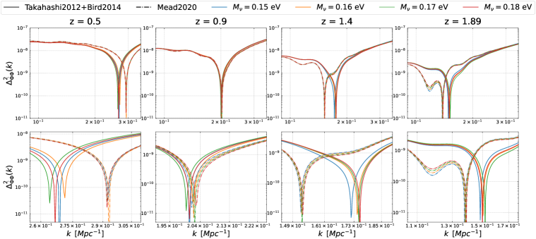
Figure 15: Top: Dimensionless and scaled form of the ISWRS–CMB-lensing potential cross-spectra as a function of the wavenumber $k$ at $z=0.5,0.9,1.4,1.89$ for $M_{\nu}=0.15,0.16,0.17,0.18$ eV (blue, yellow, green and red lines, respectively), obtained via the Takahashi2012+Bird2014 model (solid lines) and the Mead2020 model (dashed lines). Bottom: Zoom of the top panels on the sign inversions.

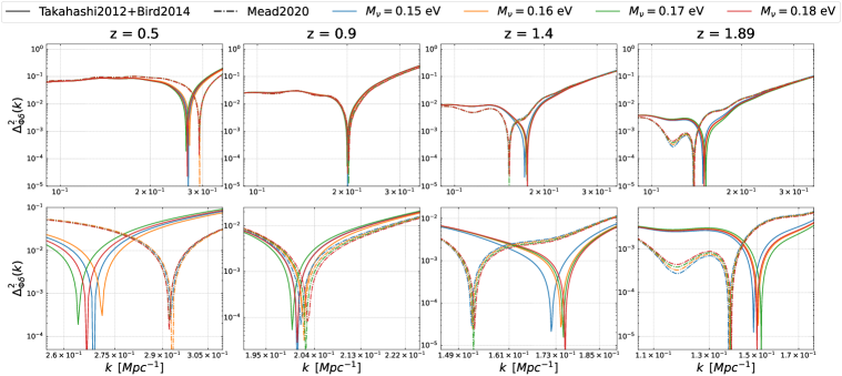
Figure 16: Top: Dimensionless and scaled form of the ISWRS–galaxy distribution cross-spectra as a function of the wavenumber $k$ at $z=0.5,0.9,1.4,1.89$ for $M_{\nu}=0.15,0.16,0.17,0.18$ eV (blue, yellow, green and red lines, respectively), obtained via the Takahashi2012+Bird2014 model (solid lines) and the Mead2020 model (dashed lines). Bottom: Zoom of the top panels on the sign inversions.

Appendix B Cosmic Variance (massless neutrino case)

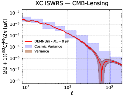
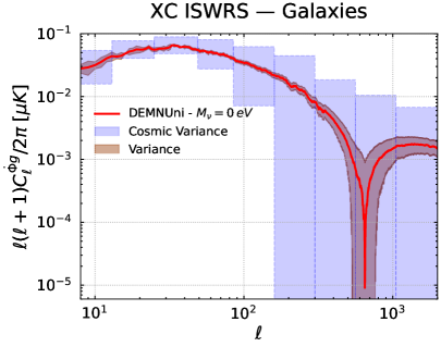
Figure 17: Left: ISWRS–CMB-lensing potential cross-spectrum for $M_{\nu}=0\text{ eV}$ (red line) with its cosmic variance binned in fourteen logarithmic equispaced intervals (shaded blue area) and the variance obtained as the standard deviation of the 5000 realisations computed (shaded brown area). Right: Same as left, but for the ISWRS–galaxy cross-spectrum for $M_{\nu}=0\text{ eV}$. In both panels, because of the choice to represent signals in range $\ell=[10,2000]$, only eleven bins are shown.

We assess the uncertainty associated to the cross-spectra in terms of cosmic variance [21, 98]:

$$\sigma_{C_{\ell}}=\sqrt{\frac{2(C_{\ell})^{2}}{2\ell+1}}\,.$$ (B.1)

For the computation of the cosmic variance of the cross-correlation of the ISWRS signal with the CMB-lensing potential and the galaxy distribution, we divide the signal variance ($\sigma$) in logarithmic equispaced bins $\Delta_{\ell_{bin_{i}}}$:

$$\sigma_{C_{\ell}^{\dot{\Phi}\Phi},\,bin_{i}}=\sqrt{\frac{(C_{\ell}^{\dot{\Phi}\Phi})^{2}+C_{\ell}^{TT}C_{\ell}^{\Phi\Phi}}{(2\ell+1)\Delta\ell_{bin_{i}}}}\,,$$ (B.2)

$$\sigma_{C_{\ell}^{\dot{\Phi}g},\hskip 2.84526ptbin_{i}}=\sqrt{\frac{(C_{\ell}^{\dot{\Phi}g})^{2}+C_{\ell}^{TT}(C_{\ell}^{gg}+N^{gg})}{(2\ell+1)\Delta\ell_{bin_{i}}}}\,.$$ (B.3)

The $C_{\ell}^{TT}$ that appears in Equation (B.2) and Equation (B.3) is the auto-power spectrum of CMB temperature primary anisotropies. Working with $C_{\ell}^{TT}$ instead of $C_{\ell}^{\dot{\Phi}\dot{\Phi}}$ arises from the fact that any CMB measurement is dominated by primary anisotropies, which are the main obstacle for a correct reconstruction of the ISWRS signal, and of secondary anisotropies in general. The $N^{gg}$ term in Equation (B.3) is the shot-noise spectrum. In this analysis, only the cosmic variance for the massless neutrino case of both the cross-spectra analysed has been computed. Moreover, we compared it with the standard deviation of 5000 realisations we computed for the two signals. Results are shown in Figure 17. The significant difference between the cosmic variance and the mocks variance is due to the fact that the 5000 gaussian realizations represent the same sky realization of the mocks, and consequently their scatter is small. Anyway, it is easy to notice that, in both panels, the larger variance values are in the larger multipole range, therefore the detection of $\ell_{inv}$ is highly unlikely.

References

- [1] A.A. Penzias and R.W. Wilson, A Measurement of Excess Antenna Temperature at 4080 Mc/s., ApJ 142 (1965) 419.
- [2] C.L. Bennett, M. Halpern, G. Hinshaw, N. Jarosik, A. Kogut, M. Limon et al., First-Year Wilkinson Microwave Anisotropy Probe (WMAP) Observations: Preliminary Maps and Basic Results, ApJS 148 (2003) 1 [astro-ph/0302207].
- [3] D.N. Spergel, L. Verde, H.V. Peiris, E. Komatsu, M.R. Nolta, C.L. Bennett et al., First-Year Wilkinson Microwave Anisotropy Probe (WMAP) Observations: Determination of Cosmological Parameters, ApJS 148 (2003) 175 [astro-ph/0302209].
- [4] E. Komatsu, K.M. Smith, J. Dunkley, C.L. Bennett, B. Gold, G. Hinshaw et al., Seven-year Wilkinson Microwave Anisotropy Probe (WMAP) Observations: Cosmological Interpretation, ApJS 192 (2011) 18 [1001.4538].
- [5] Planck Collaboration, P.A.R. Ade, N. Aghanim, C. Armitage-Caplan, M. Arnaud, M. Ashdown et al., Planck 2013 results. XVI. Cosmological parameters, A&A 571 (2014) A16 [1303.5076].
- [6] Planck Collaboration, P.A.R. Ade, N. Aghanim, M. Arnaud, M. Ashdown, J. Aumont et al., Planck 2015 results. XIII. Cosmological parameters, A&A 594 (2016) A13 [1502.01589].
- [7] Planck Collaboration, N. Aghanim, Y. Akrami, M. Ashdown, J. Aumont, C. Baccigalupi et al., Planck 2018 results. VI. Cosmological parameters, A&A 641 (2020) A6 [1807.06209].
- [8] E.V. Linder, Exploring the Expansion History of the Universe, Phys. Rev. Lett. 90 (2003) 091301 [astro-ph/0208512].
- [9] J. Lesgourgues and S. Pastor, Neutrino mass from Cosmology, arXiv e-prints (2012) arXiv:1212.6154 [1212.6154].
- [10] M. Archidiacono, S. Hannestad and J. Lesgourgues, What will it take to measure individual neutrino mass states using cosmology?, J. Cosmology Astropart. Phys 2020 (2020) 021 [2003.03354].
- [11] R.K. Sachs and A.M. Wolfe, Perturbations of a Cosmological Model and Angular Variations of the Microwave Background, ApJ 147 (1967) 73.
- [12] M.J. Rees and D.W. Sciama, Large-scale Density Inhomogeneities in the Universe, Nature 217 (1968) 511.
- [13] S. Ferraro, B.D. Sherwin and D.N. Spergel, WISE measurement of the integrated Sachs-Wolfe effect, Phys. Rev. D 91 (2015) 083533 [1401.1193].
- [14] J.R. Bond, G. Efstathiou and J. Silk, Massive neutrinos and the large-scale structure of the universe, Phys. Rev. Lett. 45 (1980) 1980.
- [15] R.G. Crittenden and N. Turok, Looking for a Cosmological Constant with the Rees-Sciama Effect, Phys. Rev. Lett. 76 (1996) 575 [astro-ph/9510072].
- [16] R. Kneissl, R. Egger, G. Hasinger, A.M. Soltan and J. Truemper, Search for correlations between COBE DMR and ROSAT PSPC all-sky survey data., A&A 320 (1997) 685 [astro-ph/9610160].
- [17] S.P. Boughn, R.G. Crittenden and N.G. Turok, Correlations between the cosmic X-ray and microwave backgrounds: constraints on a cosmological constant, New A 3 (1998) 275 [astro-ph/9704043].
- [18] S.P. Boughn and R.G. Crittenden, Cross Correlation of the Cosmic Microwave Background with Radio Sources: Constraints on an Accelerating Universe, Phys. Rev. Lett. 88 (2001) 021302 [astro-ph/0111281].
- [19] S. Boughn and R. Crittenden, A correlation between the cosmic microwave background and large-scale structure in the Universe, Nature 427 (2004) 45 [astro-ph/0305001].
- [20] T. Giannantonio, R. Scranton, R.G. Crittenden, R.C. Nichol, S.P. Boughn, A.D. Myers et al., Combined analysis of the integrated Sachs-Wolfe effect and cosmological implications, Phys. Rev. D 77 (2008) 123520 [0801.4380].
- [21] J. Lesgourgues, W. Valkenburg and E. Gaztañaga, Constraining neutrino masses with the integrated-Sachs-Wolfe-galaxy correlation function, Phys. Rev. D 77 (2008) 063505 [0710.5525].
- [22] M. Douspis, P.G. Castro, C. Caprini and N. Aghanim, Optimising large galaxy surveys for ISW detection, A&A 485 (2008) 395 [0802.0983].
- [23] Y.-C. Cai, S. Cole, A. Jenkins and C. Frenk, Towards accurate modelling of the integrated Sachs-Wolfe effect: the non-linear contribution, MNRAS 396 (2009) 772 [0809.4488].
- [24] A.J. Nishizawa, The integrated Sachs-Wolfe effect and the Rees-Sciama effect, Progress of Theoretical and Experimental Physics 2014 (2014) 06B110 [1404.5102].
- [25] C. Carbone, M. Petkova and K. Dolag, DEMNUni: ISW, Rees-Sciama, and weak-lensing in the presence of massive neutrinos, J. Cosmology Astropart. Phys 2016 (2016) 034 [1605.02024].
- [26] A. Lewis and A. Challinor, “CAMB: Code for Anisotropies in the Microwave Background.” Astrophysics Source Code Library, record ascl:1102.026, Feb., 2011.
- [27] R.E. Smith, J.A. Peacock, A. Jenkins, S.D.M. White, C.S. Frenk, F.R. Pearce et al., Stable clustering, the halo model and non-linear cosmological power spectra, MNRAS 341 (2003) 1311 [astro-ph/0207664].
- [28] A. Cooray and R. Sheth, Halo models of large scale structure, Phys. Rep. 372 (2002) 1 [astro-ph/0206508].
- [29] R. Takahashi, M. Sato, T. Nishimichi, A. Taruya and M. Oguri, Revising the Halofit Model for the Nonlinear Matter Power Spectrum, ApJ 761 (2012) 152 [1208.2701].
- [30] S. Bird, M. Viel and M.G. Haehnelt, Massive neutrinos and the non-linear matter power spectrum, MNRAS 420 (2012) 2551 [1109.4416].
- [31] A.J. Mead, S. Brieden, T. Tröster and C. Heymans, HMCODE-2020: improved modelling of non-linear cosmological power spectra with baryonic feedback, MNRAS 502 (2021) 1401 [2009.01858].
- [32] A.J. Mead, J.A. Peacock, C. Heymans, S. Joudaki and A.F. Heavens, An accurate halo model for fitting non-linear cosmological power spectra and baryonic feedback models, MNRAS 454 (2015) 1958 [1505.07833].
- [33] R. Laureijs, J. Amiaux, S. Arduini, J.L. Auguères, J. Brinchmann, R. Cole et al., Euclid Definition Study Report, arXiv e-prints (2011) arXiv:1110.3193 [1110.3193].
- [34] Euclid Collaboration, A. Blanchard, S. Camera, C. Carbone, V.F. Cardone, S. Casas et al., Euclid preparation. VII. Forecast validation for Euclid cosmological probes, A&A 642 (2020) A191 [1910.09273].
- [35] Euclid Collaboration, R. Scaramella, J. Amiaux, Y. Mellier, C. Burigana, C.S. Carvalho et al., Euclid preparation. I. The Euclid Wide Survey, A&A 662 (2022) A112 [2108.01201].
- [36] M. Santos, P. Bull, D. Alonso, S. Camera, P. Ferreira, G. Bernardi et al., Cosmology from a SKA HI intensity mapping survey, in Advancing Astrophysics with the Square Kilometre Array (AASKA14), p. 19, Apr., 2015, DOI [1501.03989].
- [37] D. Kirk, F.B. Abdalla, A. Benoit-Lévy, P. Bull and B. Joachimi, Cross correlation surveys with the Square Kilometre Array, in Advancing Astrophysics with the Square Kilometre Array (AASKA14), p. 20, Apr., 2015, DOI [1501.03848].
- [38] I. Harrison, S. Camera, J. Zuntz and M.L. Brown, SKA weak lensing - I. Cosmological forecasts and the power of radio-optical cross-correlations, MNRAS 463 (2016) 3674 [1601.03947].
- [39] S. Camera, A. Raccanelli, P. Bull, D. Bertacca, X. Chen, P. Ferreira et al., Cosmology on the Largest Scales with the SKA, in Advancing Astrophysics with the Square Kilometre Array (AASKA14), p. 25, Apr., 2015, DOI [1501.03851].
- [40] M. Brown, D. Bacon, S. Camera, I. Harrison, B. Joachimi, R.B. Metcalf et al., Weak gravitational lensing with the Square Kilometre Array, in Advancing Astrophysics with the Square Kilometre Array (AASKA14), p. 23, Apr., 2015, DOI [1501.03828].
- [41] A. Weltman, P. Bull, S. Camera, K. Kelley, H. Padmanabhan, J. Pritchard et al., Fundamental physics with the Square Kilometre Array, PASA 37 (2020) e002 [1810.02680].
- [42] D.J. Schwarz, D. Bacon, S. Chen, C. Clarkson, D. Huterer, M. Kunz et al., Testing foundations of modern cosmology with SKA all-sky surveys, in Advancing Astrophysics with the Square Kilometre Array (AASKA14), p. 32, Apr., 2015, DOI [1501.03820].
- [43] K.N. Abazajian, P. Adshead, Z. Ahmed, S.W. Allen, D. Alonso, K.S. Arnold et al., CMB-S4 Science Book, First Edition, arXiv e-prints (2016) arXiv:1610.02743 [1610.02743].
- [44] K. Abazajian, A. Abdulghafour, G.E. Addison, P. Adshead, Z. Ahmed, M. Ajello et al., Snowmass 2021 CMB-S4 White Paper, arXiv e-prints (2022) arXiv:2203.08024 [2203.08024].
- [45] S. Ferraro, E. Schaan and E. Pierpaoli, Is the Rees-Sciama effect detectable by the next generation of cosmological experiments?, arXiv e-prints (2022) arXiv:2205.10332 [2205.10332].
- [46] T. Giannantonio, R. Crittenden, R. Nichol and A.J. Ross, The significance of the integrated Sachs-Wolfe effect revisited, MNRAS 426 (2012) 2581 [1209.2125].
- [47] W.A. Watson, J.M. Diego, S. Gottlöber, I.T. Iliev, A. Knebe, E. Martínez-González et al., The Jubilee ISW project - I. Simulated ISW and weak lensing maps and initial power spectra results, MNRAS 438 (2014) 412 [1307.1712].
- [48] K. Naidoo, P. Fosalba, L. Whiteway and O. Lahav, Full-sky integrated Sachs-Wolfe maps for the MICE grand challenge lightcone simulation, MNRAS 506 (2021) 4344 [2103.14654].
- [49] Y.-C. Cai, S. Cole, A. Jenkins and C.S. Frenk, Full-sky map of the ISW and Rees-Sciama effect from Gpc simulations, MNRAS 407 (2010) 201 [1003.0974].
- [50] G. Rossi, N. Palanque-Delabrouille, A. Borde, M. Viel, C. Yèche, J.S. Bolton et al., Suite of hydrodynamical simulations for the Lyman- forest with massive neutrinos, A&A 567 (2014) A79 [1401.6464].
- [51] A.J. Nishizawa, E. Komatsu, N. Yoshida, R. Takahashi and N. Sugiyama, Cosmic Microwave Background-Weak Lensing Correlation: Analytical and Numerical Study of Nonlinearity and Implications for Dark Energy, ApJ 676 (2008) L93 [0711.1696].
- [52] U. Seljak, Rees-Sciama Effect in a Cold Dark Matter Universe, ApJ 460 (1996) 549 [astro-ph/9506048].
- [53] R.E. Smith, C. Hernández-Monteagudo and U. Seljak, Impact of scale dependent bias and nonlinear structure growth on the integrated Sachs-Wolfe effect: Angular power spectra, Phys. Rev. D 80 (2009) 063528 [0905.2408].
- [54] A. Mangilli and L. Verde, Non-Gaussianity and the CMB bispectrum: Confusion between primordial and lensing-Rees-Sciama contribution?, Phys. Rev. D 80 (2009) 123007 [0906.2317].
- [55] E. Castorina, C. Carbone, J. Bel, E. Sefusatti and K. Dolag, DEMNUni: the clustering of large-scale structures in the presence of massive neutrinos, J. Cosmology Astropart. Phys 2015 (2015) 043 [1505.07148].
- [56] M. Moresco, F. Marulli, L. Moscardini, E. Branchini, A. Cappi, I. Davidzon et al., The VIMOS Public Extragalactic Redshift Survey (VIPERS) . Exploring the dependence of the three-point correlation function on stellar mass and luminosity at 0.5 <z < 1.1, A&A 604 (2017) A133 [1603.08924].
- [57] M. Zennaro, J. Bel, J. Dossett, C. Carbone and L. Guzzo, Cosmological constraints from galaxy clustering in the presence of massive neutrinos, MNRAS 477 (2018) 491 [1712.02886].
- [58] R. Ruggeri, E. Castorina, C. Carbone and E. Sefusatti, DEMNUni: massive neutrinos and the bispectrum of large scale structures, J. Cosmology Astropart. Phys 2018 (2018) 003 [1712.02334].
- [59] J. Bel, A. Pezzotta, C. Carbone, E. Sefusatti and L. Guzzo, Accurate fitting functions for peculiar velocity spectra in standard and massive-neutrino cosmologies, A&A 622 (2019) A109 [1809.09338].
- [60] G. Parimbelli, S. Anselmi, M. Viel, C. Carbone, F. Villaescusa-Navarro, P.S. Corasaniti et al., The effects of massive neutrinos on the linear point of the correlation function, J. Cosmology Astropart. Phys 2021 (2021) 009 [2007.10345].
- [61] G. Parimbelli, C. Carbone, J. Bel, B. Bose, M. Calabrese, E. Carella et al., DEMNUni: comparing nonlinear power spectra prescriptions in the presence of massive neutrinos and dynamical dark energy, J. Cosmology Astropart. Phys 2022 (2022) 041 [2207.13677].
- [62] P. Baratta, J. Bel, S. Gouyou Beauchamps and C. Carbone, COVMOS: a new Monte Carlo approach for galaxy clustering analysis, arXiv e-prints (2022) arXiv:2211.13590 [2211.13590].
- [63] M. Guidi, A. Veropalumbo, E. Branchini, A. Eggemeier and C. Carbone, Modelling the next-to-leading order matter three-point correlation function using FFTLog, arXiv e-prints (2022) arXiv:2212.07382 [2212.07382].
- [64] S. Gouyou Beauchamps, P. Baratta, S. Escoffier, W. Gillard, J. Bel, J. Bautista et al., Cosmological inference including massive neutrinos from the matter power spectrum: biases induced by uncertainties in the covariance matrix, arXiv e-prints (2023) arXiv:2306.05988 [2306.05988].
- [65] E. Carella, C. Carbone, M. Zennaro, G. Girelli, M. Bolzonella, F. Marulli et al., DEMNUni: The galaxy-halo connection in the presence of dynamical dark energy and massive neutrinos, In prep .
- [66] M. Roncarelli, C. Carbone and L. Moscardini, The effect of massive neutrinos on the Sunyaev-Zel’dovich and X-ray observables of galaxy clusters, MNRAS 447 (2015) 1761 [1409.4285].
- [67] G. Fabbian, M. Calabrese and C. Carbone, CMB weak-lensing beyond the Born approximation: a numerical approach, J. Cosmology Astropart. Phys 2018 (2018) 050 [1702.03317].
- [68] B. Hernández-Molinero, C. Carbone, R. Jimenez and C. Peña Garay, Cosmic Background Neutrinos Deflected by Gravity: DEMNUni Simulation Analysis, arXiv e-prints (2023) arXiv:2301.12430 [2301.12430].
- [69] C.D. Kreisch, A. Pisani, C. Carbone, J. Liu, A.J. Hawken, E. Massara et al., Massive neutrinos leave fingerprints on cosmic voids, MNRAS 488 (2019) 4413 [1808.07464].
- [70] N. Schuster, N. Hamaus, A. Pisani, C. Carbone, C.D. Kreisch, G. Pollina et al., The bias of cosmic voids in the presence of massive neutrinos, J. Cosmology Astropart. Phys 2019 (2019) 055 [1905.00436].
- [71] G. Verza, A. Pisani, C. Carbone, N. Hamaus and L. Guzzo, The void size function in dynamical dark energy cosmologies, J. Cosmology Astropart. Phys 2019 (2019) 040 [1906.00409].
- [72] G. Verza, C. Carbone and A. Renzi, The Halo Bias inside Cosmic Voids, ApJ 940 (2022) L16 [2207.04039].
- [73] G. Verza, C. Carbone, A. Pisani and A. Renzi, DEMNUni: disentangling dark energy from massive neutrinos with the void size function, arXiv e-prints (2022) arXiv:2212.09740 [2212.09740].
- [74] P. Vielzeuf, M. Calabrese, C. Carbone, G. Fabbian and C. Baccigalupi, DEMNUni: The imprint of massive neutrinos on the cross-correlation between cosmic voids and CMB lensing, arXiv e-prints (2023) arXiv:2303.10048 [2303.10048].
- [75] M. Zennaro, J. Bel, F. Villaescusa-Navarro, C. Carbone, E. Sefusatti and L. Guzzo, Initial conditions for accurate N-body simulations of massive neutrino cosmologies, MNRAS 466 (2017) 3244 [1605.05283].
- [76] V. Springel, The cosmological simulation code GADGET-2, MNRAS 364 (2005) 1105 [astro-ph/0505010].
- [77] M. Viel, M.G. Haehnelt and V. Springel, The effect of neutrinos on the matter distribution as probed by the intergalactic medium, J. Cosmology Astropart. Phys 2010 (2010) 015 [1003.2422].
- [78] K.M. Górski, E. Hivon, A.J. Banday, B.D. Wandelt, F.K. Hansen, M. Reinecke et al., HEALPix: A Framework for High-Resolution Discretization and Fast Analysis of Data Distributed on the Sphere, ApJ 622 (2005) 759 [astro-ph/0409513].
- [79] C. Carbone, V. Springel, C. Baccigalupi, M. Bartelmann and S. Matarrese, Full-sky maps for gravitational lensing of the cosmic microwave background, MNRAS 388 (2008) 1618 [0711.2655].
- [80] B.M. Schäfer and M. Bartelmann, Weak lensing in the second post-Newtonian approximation: gravitomagnetic potentials and the integrated Sachs-Wolfe effect, MNRAS 369 (2006) 425 [astro-ph/0502208].
- [81] B.M. Schäfer, Mixed three-point correlation functions of the non-linear integrated Sachs-Wolfe effect and their detectability, MNRAS 388 (2008) 1394 [0803.1095].
- [82] M. Calabrese, C. Carbone, G. Fabbian, M. Baldi and C. Baccigalupi, Multiple lensing of the cosmic microwave background anisotropies, J. Cosmology Astropart. Phys 2015 (2015) 049 [1409.7680].
- [83] P. Fosalba, E. Gaztañaga, F.J. Castander and M. Manera, The onion universe: all sky lightcone simulations in spherical shells, MNRAS 391 (2008) 435 [0711.1540].
- [84] S. Hilbert, A. Barreira, G. Fabbian, P. Fosalba, C. Giocoli, S. Bose et al., The accuracy of weak lensing simulations, MNRAS 493 (2020) 305 [1910.10625].
- [85] B.P. Moster, R.S. Somerville, C. Maulbetsch, F.C. Van den Bosch, A.V. Macciò, T. Naab et al., Constraints on the relationship between stellar mass and halo mass at low and high redshift, ApJ 710 (2010) 903 [0903.4682].
- [86] F. Shankar, A. Lapi, P. Salucci, G. De Zotti and L. Danese, New Relationships between Galaxy Properties and Host Halo Mass, and the Role of Feedbacks in Galaxy Formation, ApJ 643 (2006) 14 [astro-ph/0601577].
- [87] G. Girelli, L. Pozzetti, M. Bolzonella, C. Giocoli, F. Marulli and M. Baldi, The stellar-to-halo mass relation over the past 12 Gyr. I. Standard CDM model, A&A 634 (2020) A135 [2001.02230].
- [88] I. Tutusaus, M. Martinelli, V.F. Cardone, S. Camera, S. Yahia-Cherif, S. Casas et al., Euclid: The importance of galaxy clustering and weak lensing cross-correlations within the photometric Euclid survey, A&A 643 (2020) A70 [2005.00055].
- [89] C. Modi, S.-F. Chen and M. White, Simulations and symmetries, MNRAS 492 (2020) 5754 [1910.07097].
- [90] M. Calabrese, C. Carbone, E. Carella et al., Mock simulations for cmb cross-correlation (in prep.), .
- [91] F. Marulli, C. Carbone, M. Viel, L. Moscardini and A. Cimatti, Effects of massive neutrinos on the large-scale structure of the Universe, MNRAS 418 (2011) 346 [1103.0278].
- [92] L. Xu, Probing the neutrino mass through the cross correlation between the Rees-Sciama effect and weak lensing, J. Cosmology Astropart. Phys 2016 (2016) 059 [1605.02403].
- [93] T. Giannantonio, R.G. Crittenden, R.C. Nichol, R. Scranton, G.T. Richards, A.D. Myers et al., High redshift detection of the integrated Sachs-Wolfe effect, Phys. Rev. D 74 (2006) 063520 [astro-ph/0607572].
- [94] A. Lee, M.H. Abitbol and S. Adachi et al., The Simons Observatory, in Bulletin of the American Astronomical Society, vol. 51, p. 147, Sept., 2019 [1907.08284].
- [95] LiteBIRD Collaboration, E. Allys, K. Arnold, J. Aumont, R. Aurlien, S. Azzoni et al., Probing cosmic inflation with the LiteBIRD cosmic microwave background polarization survey, Progress of Theoretical and Experimental Physics 2023 (2023) 042F01 [2202.02773].
- [96] T. Eifler, H. Miyatake, E. Krause, C. Heinrich, V. Miranda, C. Hirata et al., Cosmology with the Roman Space Telescope - multiprobe strategies, MNRAS 507 (2021) 1746 [2004.05271].
- [97] Ž. Ivezić, S.M. Kahn and J.A.T. et al., LSST: From science drivers to reference design and anticipated data products, The Astrophysical Journal 873 (2019) 111.
- [98] U. Seljak, N. Hamaus and V. Desjacques, How to Suppress the Shot Noise in Galaxy Surveys, Phys. Rev. Lett. 103 (2009) 091303 [0904.2963].