Impact Rates in the Outer Solar System

Abstract

Previous studies of cometary impacts in the outer Solar System used the spatial distribution of ecliptic comets (ECs) from dynamical models that assumed ECs began on low-inclination orbits ($\lesssim 5^{\circ}$) in the Kuiper belt (Levison and Duncan, 1997). In reality, the source population of ECs – the trans-Neptunian scattered disk – has orbital inclinations reaching up to $\sim 30^{\circ}$ (Di Sisto and Rossignoli, 2020). In Nesvorný et al. (2017), we developed a new dynamical model of ECs by following comets as they evolved from the scattered disk to the inner Solar System. The model was absolutely calibrated from the population of Centaurs (Nesvorný et al., 2019) and active ECs. Here we use our EC model to determine the steady-state impact flux of cometary/Centaur impactors on Jupiter, Saturn, Uranus, and their moons. Relative to previous work (Zahnle et al., 2003), we find slightly higher impact probabilities on the outer moons and lower impact probabilities on the inner moons. The impact probabilities are smaller when comet disruption is accounted for. The results provide a modern framework for the interpretation of the cratering record in the outer Solar System.

1 Introduction

Comets are icy objects that reach the inner Solar System after leaving distant reservoirs beyond Neptune and are dynamically evolving onto elongated orbits with small perihelion distances (see Dones et al. (2015) and Kaib & Volk (2023) for recent reviews). Their activity, manifesting itself by the presence of a dust/gas coma and tail, is driven largely by solar heating and sublimation of various ices. Once they reach the inner Solar System, comets are short-lived, implying that they must be resupplied from external reservoirs. Here we focus on the ecliptic comets (ECs – low-to-moderate inclination planet-crossing bodies in the region of the giant planets; see Levison and Duncan (1997) and Fraser et al. (2023) for further discussion) because (1) the population of ECs is relatively well characterized from observations and allows us to construct a realistic model (Section 2), and (2) ECs, and their Centaur precursors, are more important for impact cratering in the outer Solar System than other types of comets (e.g., long-period comets; LPCs), escaped asteroids and Trojans (e.g., Levison et al. (2000), Zahnle et al. (1998), Zahnle et al. (2001), and Zahnle et al. (2003) [hereafter Z03]).

Levison and Duncan (1997) [hereafter LD97] considered the origin and evolution of ecliptic comets. LD97 assumed that the classical Kuiper belt 30–50 au from the Sun was the main source of ECs. They showed that small Kuiper belt objects (KBOs) reaching Neptune-crossing orbits can be scattered by encounters with the outer planets to small perihelion distances ($q<2.5$ au), at which point they are assumed to become active and visible Jupiter-family comets (JFCs). The JFCs reaching $q<2.5$ au for the first time have a narrow inclination distribution in the LD97 model, because the orbits were assumed to start with low inclinations in the Kuiper belt and the inclinations changed little before the comets reached Jupiter-crossing orbits. Levison and Duncan (1994) and LD97 pointed out that the inclination distribution of JFCs widens over time due to scattering encounters with Jupiter. LD97 found their best fit to the observed inclination distribution of JFCs (median $\simeq 13^{\circ}$) when they assumed that ECs remain active for $\simeq 12$,000 years (with a range of 3,000 to 30,000 years) after first reaching $q<2.5$ au.

The escape of ECs from the classical Kuiper belt is driven by slow chaotic processes in various orbital resonances with Neptune. Because these processes affect only part of the belt, with most orbits being stable for billions of years, comet delivery from the classical Kuiper belt is inefficient (Nesvorný et al. 2017). Duncan and Levison (1997) suggested that the scattered disk, whose prototype is (15874) 1996 TL66 (semi-major axis $a=134$ au, $q=35$ au; Luu et al. (1997)), should be a more prolific source of ECs. This is because scattered disk objects (SDOs) can approach Neptune during their perihelion passages and be scattered by Neptune to orbits with shorter orbital periods, implying a faster loss rate for SDOs than for classical KBOs (Duncan et al., 2004). The population of SDOs is also inferred to be larger than that of classical KBOs ($\sim 0.05$ $M_{\earth}$ vs. $\sim 0.01$ $M_{\earth}$; Fraser et al. (2014), Nesvorný (2018)) thus representing a large source for ECs.

Z03 used the spatial distribution of ECs from LD97 to determine impact rates in the outer Solar System. They estimated that the current rate at which EC nuclei with diameters $D>1.5$ km strike Jupiter is $0.005^{+0.006}_{-0.003}$ yr^-1. Z03’s rate for Jupiter was based on considerations such as four known passages of JFCs within 3 jovian radii in the past 150 years and models of the population of near-Earth JFCs from LD97. Z03 then calculated impact rates on Saturn, Uranus, and Neptune by scaling from the rate on Jupiter using LD97’s model. Impact rates on the satellites of the giant planets were, in turn, calculated by Z03 with an Öpik-like formalism (Öpik, 1951). The main uncertainties in the impact rates given in Z03 arise from: (1) the assumed source reservoir in LD97, and hence the spatial distribution of ECs (see discussion above); (2) our poor understanding of the sizes of the nuclei of active ECs; (3) the approximate nature of the impact flux calculation in LD97 (see Levison et al. (2000)); and (4) the small number of direct impacts recorded on each planet in LD97. As for (2), a common procedure is to infer the diameter $D$ of a comet nucleus from its absolute magnitude $H_{\rm T}$, which quantifies the total brightness of a comet, including coma, at a standard distance of 1 au from the Earth and Sun (e.g., Brasser & Morbidelli (2013)). The nature of the relation between $H_{\rm T}$ and $D$ is, however, uncertain because comets vary greatly in their levels of activity.

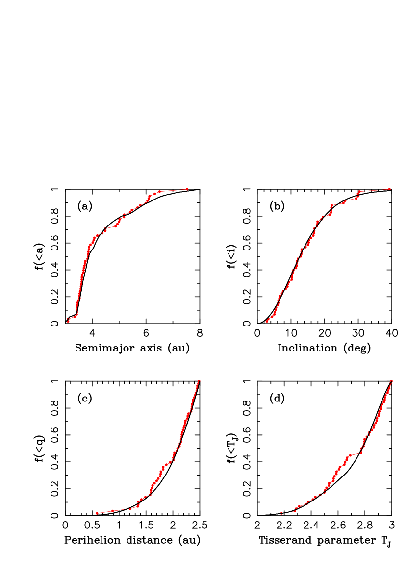
An important prerequisite for the interpretation of the cratering record in the outer Solar System is to have a reliable model of ECs. We developed such a model in Nesvorný et al. (2017) (hereafter N17). In N17, we performed end-to-end simulations in which cometary reservoirs, including the scattered disk and Oort cloud, were produced in the early Solar System and evolved for 4.5 Gyr. The simulations included the effects of the four giant planets. The model was calibrated from the observed population of active ECs, but includes other types of comets as well. We considered different scenarios for the duration of cometary activity, including a simple model in which comets remain active for $N_{\rm p}(q)$ perihelion passages with perihelion distance $q<2.5$ au. To constrain $N_{\rm p}(2.5)$, we compared the orbital distribution and number of active comets produced in the model to observations. The observed distribution was well reproduced with $N_{\rm p}(2.5)\simeq 300$–800 (see Fig. 1 here). Here we adopt $N_{\rm p}(2.5)\simeq 600$ as a reference value for comets with $D\sim 1$ km (N17 inferred that $N_{\rm p}(2.5)$ should increase with the size of the nucleus). As the median orbital period of ECs is $\simeq 8$ yr (N17), our reference value corresponds to $\simeq 4$,800 yr – a factor of 2.5 shorter than the nominal LD97 estimate. Ultimately, this is a consequence of new ECs (i.e., bodies reaching Jupiter-crossing orbit for the first time) having a wider inclination distribution in the N17 model because they start with larger inclinations in the scattered disk.

The main uncertainty in the N17 model was related to the absolute calibration. N17 used Jupiter Trojans, whose size distribution is well characterized from observations down to $D\sim 3$ km (Wong and Brown, 2015; Yoshida and Terai, 2017), for this purpose. This method relies on the assumption that the Trojan implantation efficiency from the original planetesimal disk is relatively well determined (Morbidelli et al., 2005; Nesvorný et al., 2013). We modeled the collisional evolution of Jupiter Trojans and SDOs and found that the size distribution changes after their implantation were insignificant (Nesvorný et al., 2018; Bottke et al., 2023). In addition, Pluto/Charon craters indicate that the size distribution slope of impactors with $D>1$ km in the Kuiper belt is similar to that of Jupiter Trojans (Singer et al., 2019). The use of the Trojan size distribution to model comets may therefore be justified.

2 Method

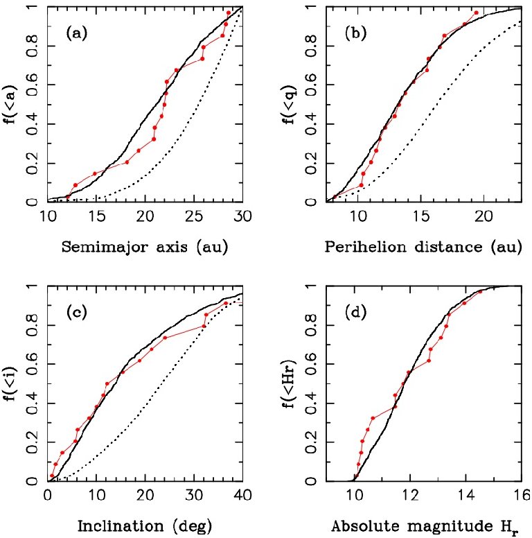
A better calibration of planetary impactors in the outer Solar System is provided by the Outer Solar System Origins Survey (OSSOS; Bannister et al. (2018)) observations of Centaurs (Dorsey et al. 2023, Cabral et al. 2019). In Nesvorný et al. (2019), we used the N17 model to predict the orbital distribution and the number of Centaurs. The model distribution was biased by the OSSOS simulator and compared with the OSSOS Centaur detections. We found a good fit to the observed orbital distribution, including the wide range of orbital inclinations, which was the hardest characteristic to fit in previous models (see Fig. 2 here and Marsset et al. 2019 for how the orbital inclinations of KBOs and Centaurs correlate with photometric color, and Nesvorný et al. 2020 for modeling of the inclination-color relationship). The N17 dynamical model, in which the original population of outer disk planetesimals was calibrated from Jupiter Trojans (see above), implies that OSSOS should have detected $11\pm 4$ Centaurs with semimajor axes $a<30$ au, perihelion distances $q>7.5$ au, and diameter $D>10$ km (absolute magnitude $H_{r}<13.7$ for a 6% geometric albedo). This is consistent with 15 actual OSSOS Centaur detections with $H_{r}<13.7$.

By slightly adjusting the N17 model to accurately match the OSSOS Centaur detections, Nesvorný et al. (2019) infer that the inner scattered disk at $50<a<200$ au, from where most ECs evolve (N17), should contain $(2.0\pm 0.8)\times 10^{7}$ $D>10$ km objects at the present time. This is consistent with independent estimates by Lawler et al. (2018) and Di Sisto and Rossignoli (2020). We can then rewind the history of the population using the N17 simulations to estimate that the original trans-Neptunian disk contained $(8\pm 3)\times 10^{9}$ planetesimals with $D>10$ km. Reference population estimates for smaller diameter cutoffs can be obtained from the size distribution of Jupiter Trojans: cumulative $N(D)\propto D^{-2.1}$ down to $D\sim$ 3–5 km (Grav et al. (2011); Wong and Brown (2015); Yoshida and Terai (2017); Uehata et al. (2022); see discussion in Section 3.1), and perhaps even down to $D\sim$ 1–2 km.

With the orbital model and absolute calibration in place, we can estimate the impact rates of ECs and Centaurs on the outer planets and their moons. For that purpose, we repeat the simulations in N17. Specifically, we select the best case from N17, in which Neptune started at $a_{\rm N,0}=22$ au, migrated at a rate proportional to $\exp(-t/\tau_{1})$, with $\tau_{1}=10$ Myr, for the first 10 Myr, and then at a rate $\propto\exp(-t/\tau_{2})$, with $\tau_{2}=30$ Myr, for $10<t<500$ Myr (Case 2 in N17). Time $t$ is measured from the dispersal of the protoplanetary gas disk some 4.56 Gyr ago. The dynamical instability happened at $t=10$ Myr in this case. The present properties of the EC population are not sensitive to the details of Neptune’s early migration (e.g., Nesvorný et al. 2017). The galactic tide and stellar encounters were included in the simulation, while the putative Planet Nine (Trujillo & Sheppard 2014, Batygin & Brown 2016, N17) was not.

Since we are interested in the current impact rate of ECs/Centaurs (see Wong et al. (2019), Wong et al. (2021) and Bottke et al. (2023) for impact rates in the early Solar System), we repeated the last segment of the N17 simulation, in which cometary reservoirs were evolved from 1 Gyr ago to the present time. By slicing this wide time interval into smaller segments and comparing the results, we verified that the EC/Centaur population changed little over the past 1 Gyr (e.g., the impact rate on Jupiter changes by $<10$% in the past 1 Gyr). We thus used the full statistics in the 1-Gyr long interval to infer the current impact rate. The original simulations started with $10^{6}$ test planetesimals in the disk between 24 and 30 au at $t=0$. To further improve the model statistics, we cloned test bodies as they evolved toward the inner Solar System. Specifically, in the last 1 Gyr interval, we monitored the heliocentric distance $r$ of each body, and cloned it 50 times when $r$ first dropped below $r^{*}=23$ au. This effectively corresponds to $N=5\times 10^{7}$ (initial) test planetesimals. The simulations were performed on 2000 Ivy Bridge cores of the NASA Ames Pleiades Supercomputer. We used the swift_rmvs4 integrator (Levison and Duncan, 1994) and a 0.2 yr timestep. All impacts of bodies on the outer planets were recorded by the $N$-body integrator.

To compute impact rates on the outer planets’ moons, we first recorded all encounters of model bodies within $\simeq$1 Hill radius of each planet. For every encounter, we then used Eq. (3) from Nesvorný et al. (2004) to compute the collisional probability with moons. The computation of collisional probabilities accounts for the moons’ real orbits, including their (typically small) orbital eccentricities and inclinations. We verified that, for a moon on a circular orbit, the results are consistent with the Öpik equations (Öpik (1951); Zahnle et al. (1998); Zahnle et al. (2003); see footnote 8 in Nesvorný et al. (2004)). The bodies that were bound to the planet were treated separately – their collisional probability was computed from Eq. (13) in Nesvorný et al. (2003). In most cases, dynamical and physical characteristics of moons (orbital elements, physical radii, surface gravities, etc.) were taken from the NASA JPL Planetary Satellites site. We assumed spherical shapes for all moons and accounted for the gravitational focusing of comets by moons. The reduction in outbound impactor flux due to collisions with the planet (“shielding”) was also accounted for (Lissauer et al., 1988). We accumulated the collisional probability over all recorded encounters and, following Z03, expressed it as a fractional impact probability relative to Jupiter (Tables 1–3).

We considered two ways an EC can become inactive: it becomes dormant, either because a refractory mantle forms or the comet loses all volatiles, or it breaks into small pieces and disappears. (We ignore the possibility that the comet breaks into several large fragments.) We must distinguish between these possibilities because they have different implications for the impact flux. The impact flux is expected to be higher if comets become dormant, because the nucleus is still intact. If, instead, ECs disrupt, they must be removed from the pool of impactors. Studies of meteor orbits suggest that disruption is the main physical loss mechanism for Jupiter-family comets (Ye et al., 2016). Nonetheless, we considered two end-member models. In each, we assumed that comets have a physical lifetime of $N_{\rm p}(2.5)=600$ perihelion passages within 2.5 au, as in N17 (Section 1). In the first case (Sections 3.1.1 and 3.2.1), we assumed comets became dormant and retained them in the impact flux calculation. In the second case (Sections 3.1.2 and 3.2.2), we assumed comets were disrupted and removed them from the impact flux calculation. We only model comet fading or disruption at small perihelion distances in this work (as parameterized by $N_{p}(2.5)$). Comet fading and/or disruption at larger perihelion distances (e.g., due to activity driven by supervolatiles or tidal encounters with planets) is not accounted for.

3 Results

3.1 Planetary Impacts

3.1.1 Results Without Comet Disruption

In total, our model recorded 217 direct impacts on Jupiter, 70 impacts on Saturn and 62 impacts on Uranus. We do not consider impacts on Neptune and its moons in this work. Neptune and its moons are bombarded not only by Centaurs, but also by scattered disk objects (SDOs). We do not have complete statistics for SDOs because we cloned the bodies in our model at $r^{*}=23$ au. Interestingly, 24%, 11% and 6% of the bodies were bound to Jupiter, Saturn and Uranus, respectively, at the time of impact. For Jupiter, this is close to the 21% reported in Levison et al. (2000) and $15\pm 2$% given by Kary and Dones (1996). For Jupiter, 3 out of 217 impactors ($\sim 1.4$%) had Tisserand parameters with respect to Jupiter $T_{\rm J}<2$, indicating that only 1–2% of impactors were near-isotropic comets (NICs; LD97) from the Oort cloud (Vokrouhlický et al., 2019). The great majority of impactors (98–99%) were ECs with $2<T_{\rm J}<3.05$. Ecliptic comet precursors – the low-inclination Centaurs evolving from the scattered disk – also dominate impacts on Saturn and Uranus (e.g., only one of 62 Uranus impactors had a retrograde heliocentric orbit).

The impact rate of ECs/Centaurs on Jupiter is computed as follows. Having effectively $5\times 10^{7}$ test bodies in the original trans-Neptunian disk ($10^{6}$ original planetesimals $\times$ 50 clones for bodies that reached $r^{*}=23$ in the past billion years, see Section 2), we recorded 217 impacts in 1 Gyr. According to the calibration discussed above, there were $(8\pm 3)\times 10^{9}$ planetesimals with $D>10$ km when Neptune began to migrate. The current rate of impacts of $D>10$ km bodies on Jupiter (i.e., the average for the last billion years, see Section 2) is therefore $217\times 8\times 10^{9}/(5\times 10^{7}\times 10^{9})=3.5\times 10^{-5}$ yr^-1, implying a timescale for impacts by $D>10$-km bodies $\simeq 2.9\times 10^{4}$ yr. If we adopt the reference cumulative size distribution $N(D)\propto D^{-2.1}$ from N17 (Section 2) and assume it extends down to $D=1$ km, we estimate a timescale for impacts by $D>1$-km bodies of $\simeq 230$ yr. We use this timescale as a baseline in the rest of this paper. For comparison, Dones et al. (2009) inferred the impact flux on Jupiter from the historical record of close approaches and impacts (Schenk and Zahnle, 2007). They estimated an impact rate of at least $4\times 10^{-3}$ yr^-1 for $D>1$ km, implying a timescale $\lesssim 250$ yr, which is consistent with our model results. Saturn and Uranus receive 0.32 and 0.29 of the Jupiter impact flux, respectively, implying impact timescales of $\simeq 720$ yr and $\simeq 790$ yr, respectively, for $D>1$-km impacts.

One major source of uncertainty of our model estimates is the extrapolation of the impact rate from $D>10$ km to $D>1$ km. Above, we assumed a single power-law slope of 2.1 for simplicity. Subaru telescope observations of Jupiter Trojans indicate that the cumulative power index of Jupiter Trojans changes from $\simeq 2.25$ for $D>5$ km to $\simeq 1.8$ for $D<5$ km, assuming that albedo is independent of size (e.g., Uehata et al. (2022)). If the shallower slope is extended all the way down to 1 km, we would infer a $\simeq 340$ yr timescale for impacts of $D>1$ km bodies on Jupiter, i.e., an impact rate $\sim 2/3$ of our previous estimate. It also may be that the size distribution of Jupiter Trojans is not a good proxy for cometary impactors. If we generously assume that the cometary size distribution is steeper, $N(D)\propto D^{-2.4}$, for $1<D<10$ km, based on craters on Iapetus’s dark terrain (Kirchoff & Schenk, 2010), we obtain a $\simeq 120$-yr timescale for impacts of $D>1$ km bodies on Jupiter.

3.1.2 Results With Comet Disruption

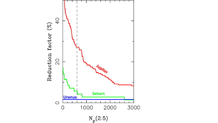
Figure 3 shows how the number of planetary impacts is reduced when we assume that comets disrupt after a certain number of orbits with $q<2.5$ au. As expected, comet disruption has the largest effect for Jupiter, where the impact rate, assuming $N_{\rm p}(2.5)=600$, is reduced by 27% from its value neglecting disruption. For Saturn and Uranus, the corresponding factors are 6% and 2%. The average time between impacts of $D>1$-km bodies on Jupiter, Saturn and Uranus is then 320, 760 and 810 yr, respectively (here and elsewhere in the paper we scale from the nominal reference timescale of 230 yr for Jupiter discussed above). For all planets, the reduction factor decreases if we assume long physical lifetimes for comets. For example, for $N_{\rm p}(2.5)=3000$, as appropriate for $D\sim 10$ km ECs from N17, the impact flux on Jupiter is reduced by only 8%.

The fraction of bound impactors is larger when comet disruption is included in the model. For example, without accounting for comet disruption, we find that 24% of Jupiter impactors were bound to Jupiter when they impacted. With $N_{\rm p}(2.5)=600$, which should be appropriate for $D\sim 1$ km comets (N17), we find that the fraction of bound impactors is $\simeq 30$%. Bound Jupiter impactors are slightly less likely to have many perihelion passages below 2.5 au than the population of ECs as a whole. Bound objects typically have $T_{\rm J}\approx 3$ (Kary and Dones, 1996). Bodies that encounter Jupiter at higher velocities, and hence have smaller Tisserand parameters, are more easily scattered by Jupiter into orbits with small perihelion distances (Levison and Duncan (1997); see Figure 9 of Fernández et al. (2018)). This means that events such as Shoemaker-Levy 9, which was tidally disrupted by Jupiter in 1992 and collided with the planet in 1994, would happen slightly more often – relative to impacts from unbound orbits – if comets disrupt.

3.2 Impacts on Moons

3.2.1 Results Without Comet Disruption

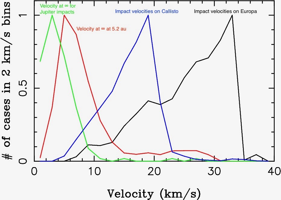
The impact probabilities on the outer planets’ moons, both with and without comet disruption, are reported in Tables 1–3. There are some notable differences from Zahnle et al. (2003). We obtain higher impact speeds for the outermost moons. For example, we find $\langle v_{\rm imp}\rangle=7.1$ km/s for Phoebe, whereas Z03 reported $\langle v_{\rm imp}\rangle=3.2$ km/s (here, $v_{\rm imp}$ is the impact speed of an individual body and $\langle v_{\rm imp}\rangle$ is the mean impact speed computed over all recorded impacts). Z03 ultimately based their encounter velocity ($v_{\infty}$, the velocity at “infinity” – in practice, the planet’s Hill sphere) distribution on objects that struck Jupiter in LD97. That distribution is biased toward low-velocity encounters because of gravitational focusing by Jupiter. In reality, there is a wide range of values of $v_{\infty}$ at each planet (Fig. 4). The outermost satellites of the giant planets have orbital velocities $v_{\rm orb}<\langle v_{\infty}\rangle$, where $\langle v_{\infty}\rangle$ is the average encounter velocity of bodies at the planet’s Hill sphere ($v_{\rm orb}$ is the orbital velocity of a moon around its parent planet). Therefore, gravitational focusing by the planet is a minor effect for them. This implies that impacts on the outer moons sample the high-velocity portion of the background velocity distribution more than do the inner moons and the planets themselves (Zahnle et al. (1998), Section 2.1).

By contrast, the inner satellites of the giant planets have orbital velocities $v_{\rm orb}>\langle v_{\infty}\rangle$. As a result, Centaurs/ECs are more strongly focused gravitationally. In the limit $v_{\rm orb}\gg\langle v_{\infty}\rangle$, the impact rate per unit area on a moon ${\cal F}_{\rm imp}\mathrel{\vbox{ \offinterlineskip\halign{\hfil$#$\cr\propto\cr\kern 2.0pt\cr\sim\cr\kern-2.0pt\cr}}}1/(a_{\rm moon}v_{\infty}^{2}$), where $a_{\rm moon}$ is the moon’s semimajor axis (see, e.g., Eq. (4) in Z03). For reference, $\langle v_{\infty}\rangle=$ 4.1 km/s for bodies that impact Jupiter, while $\langle v_{\infty}\rangle=$ 8.8 km/s for bodies that cross Jupiter’s orbit. These values are, respectively, approximately 30% and 70% of Jupiter’s mean orbital speed.

Other differences may arise from the dependence on the structure of the source regions assumed in different works. Z03 adopted the results from Levison and Duncan (1997); Levison et al. (2000), where bodies started with low inclinations in the classical Kuiper belt. This leads to a dynamically colder population of Centaur/EC impactors and lower impact speeds for more distant satellites. Here, instead, Centaurs/ECs evolve from the scattered disk in our model (N17) and so have higher inclinations and larger impact speeds.

The mean impact speeds for the inner moons that we find in this work are typically slightly smaller than the mean impact speeds given in Z03. For a monodisperse encounter velocity ($v_{\infty}$), higher impact speeds for the outer moons would imply higher impact speeds for the inner moons as well. If we approximate the distribution of $v_{\infty}$ as a Maxwellian, the impact probability weighted mean encounter velocity is $\frac{1}{2}v_{\infty}$ in the limit $v_{\rm orb}\gg\langle v_{\infty}\rangle$. The slightly lower impact speeds for the inner moons probably reflect this sampling and the different velocity distributions we and Z03 assume (see Zahnle et al. (2001), Eq. 1). Our low-velocity tail probably extends to slightly lower speeds than does that of Z03, and this tail is preferentially sampled by the inner moons.

We find higher impact rates for distant moons and lower impact rates for the innermost moons (Tables 1–3; recall that these rates are normalized to Jupiter), relative to Z03. Therefore, our impact probability profiles with orbital radius are flatter than in Z03. For example, the outer moons of Saturn have impact probabilities that are up to $\sim 2$ times higher than in Z03 (e.g., Phoebe has $P_{\rm imp}=1.8\times 10^{-8}$ here and $P_{\rm imp}=8.7\times 10^{-9}$ in Z03). The higher (normalized) impact probabilities for the outermost moons are a consequence of higher encounter velocities in our model, which result in lower gravitational focusing on the planets.

The mid-sized moons of Saturn have impact probabilities that are slightly smaller than reported in Z03 (e.g., Mimas has $P_{\rm imp}=1.7\times 10^{-6}$ in Z03 and $P_{\rm imp}=1.1\times 10^{-6}$ in this work; the impact probability $P_{\rm imp}$ is relative to Jupiter). Part of this difference results from the lower impact rates on Saturn relative to Jupiter that we find here (0.32 vs. 0.42 in Z03).

For the innermost moons (Metis–Thebe for Jupiter, Pan–Janus for Saturn, and Portia and Puck for Uranus), the differences with Z03 are larger. These result from, e.g., differences in assumed sizes for the satellites and shielding by the planet (Lissauer et al., 1988), which we account for, but Z03 did not. As an independent check, we verified that our impact probabilities for the innermost moons follow the expected scaling. For these moons, the value of $P_{\rm imp}$ should be approximately $(R_{\rm moon}/R_{\rm planet})^{2}(R_{\rm planet}/a)$, where $R_{\rm moon}$ and $R_{\rm planet}$ are the physical radii of the moon and planet, and $a$ is the semi-major axis of the moon. The first term is the ratio of cross sections, while the second term accounts for gravitational focusing by the planet.

3.2.2 Results With Comet Disruption

The impact flux is reduced when the effects of comet disruption are included in the model (Tables 1–3). The flux is reduced by $\sim 25$–45% for the jovian moons, $\sim 5$–15% for the saturnian moons, and $<1$% for the uranian moons. This trend, with the reduction factor decreasing with heliocentric distance, is expected because comet disruption mainly reduces the impactor population at smaller heliocentric distances. Compared to planetary impacts (Section 3.1), the reduction factors for moons are larger. For example, the impact flux on Jupiter was reduced by 27% from the original flux for $N_{\rm p}(2.5)=600$ (appropriate for $\sim 1$-km impactors). For jovian moons, however, the impact flux is reduced by $\sim 25$–45% for $N_{\rm p}(2.5)=600$, and there is a trend with smaller reduction for inner moons and larger reduction for outer moons.

The impact speeds on the outer moons of Jupiter are slightly lower in the case with disruption. For example, the mean impact speeds on Himalia are 8 and 9 km/s with and without disruption, respectively (Table 1). This most likely happens because in the case with disruption, there is not enough time to excite the heliocentric orbits of EC impactors as much. The effects of disruption on the impact speeds for moons of Saturn and Uranus are small (Tables 2 and 3).

The lower cratering rates in the case that includes cometary disruption imply somewhat older surface ages for lightly-cratered terrains on outer planet satellites such as Enceladus and Europa. For example, Z03 estimated the surface age of Europa between 30 and 70 Myr (more recent papers infer slightly older ages: 60–100 Myr in Zahnle et al. (2008) and 40–90 Myr in Bierhaus et al. (2009)). Scaling from Z03, our lower impact flux in the model with comet disruption would imply a surface age between 45 and 105 Myr. The catastrophic disruption timescales of small moons reported in Z03, which assume that a crater with a diameter equal to the diameter of the satellite dooms the moon, would also be longer.

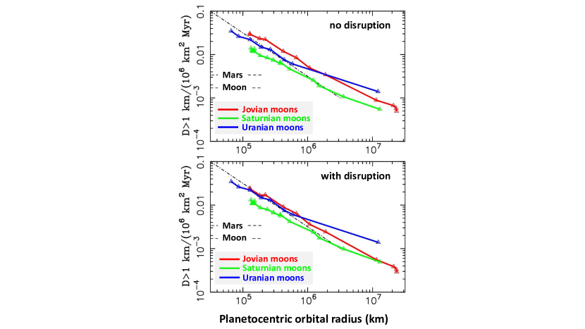
Figure 5 shows how the impact flux depends on the orbital radius of a moon. Here, we disregard the moons’ sizes by normalizing the impact flux of $D>1$ km comets per $10^{6}$ km² of the moon’s surface (per Myr). When comet disruption is not accounted for, the normalized impact flux is ${\cal F}_{\rm imp}\simeq$ 0.0005–0.002/$(10^{6}\,{\rm km}^{2}\,{\rm Myr})$ for the outer moons and ${\cal F}_{\rm imp}\simeq 0.01$–0.05/$(10^{6}\,{\rm km}^{2}\,{\rm Myr})$ for the inner moons. The higher flux on inner moons is due to gravitational focusing by the planets. This trend persists when we account for comet disruption (bottom panel of Fig. 5). Given that the flux reduction is larger for the outer moons, however, the overall slope of the ${\cal F}_{\rm imp}$ dependence on $a_{\rm moon}$ becomes slightly steeper with comet disruption. For example, the outer/irregular moons of Jupiter have ${\cal F}_{\rm imp}\simeq$ 0.0004/$(10^{6}\,{\rm km}^{2}\,{\rm Myr})$ with $N_{\rm p}(2.5)=600$ compared to ${\cal F}_{\rm imp}\simeq$ 0.0006/$(10^{6}\,{\rm km}^{2}\,{\rm Myr})$ without comet disruption.

4 Discussion

The impact flux on the satellites depends on whether comets undergo disruption or become dormant. The flux is higher if comets become dormant (Tables 1–3). We expect that both cases apply to some degree. For example, if all comets become dormant, the ratio of the number of dormant to active ECs should be roughly 30–60. This is because the dynamical lifetime of ECs with $q<2.5$ au is $t_{\rm dyn}\sim 3\times 10^{5}$ yr (LD97), while their physical lifetime is $t_{\rm phy}\sim$ 5,000–12,000 yr (LD97, N17). The ratio of the number of dormant to active ECs should be $\sim t_{\rm dyn}/t_{\rm phys}$.

Licandro et al. (2016) obtained WISE observations of asteroids on (mostly Jupiter-family-like) cometary orbits [ACOs] and inferred their size distribution. They found that the number of ACOs is smaller than the number of JFCs for diameters $<10$ km. This suggests that most ecliptic comets end their lives by being disrupted instead of becoming dormant (also see Ye et al. (2016)). Therefore, the impact fluxes that we calculate for the case with cometary disruption are likely to be more realistic. This may not be true for Centaurs, which are less likely to be disrupted because of their greater distances from the Sun.

5 Conclusions

The main results of this work can be summarized as follows:

1. We determined the current rates at which comets and Centaurs strike the moons of Jupiter, Saturn, and Uranus. Compared to Zahnle et al. (2003), we find a higher impact flux on the outer moons and a smaller impact flux on the inner moons. This is a consequence of the larger orbital inclinations in our model, in which the scattered disk is the main source of comets/Centaurs. The impact speeds on outer moons are significantly higher (e.g., 7.1 km/s for Phoebe compared to 3.2 km/s reported for Phoebe in Z03), implying larger craters for a given impactor size.

2. When comet disruption is accounted for, the impact flux on the outer planets and their moons is reduced. The reduction factor depends on the adopted disruption model. For example, for $N_{\rm p}(2.5)=600$, which was the preferred value for $D\sim 1$ km comets in Nesvorný et al. (2017), the impact flux on Jupiter is reduced to 73% of the original value (the mean interval between impacts of $D>1$ km comets on Jupiter is $\sim 230$ yr without comet disruption and $\sim 315$ yr with comet disruption).

3. For $N_{\rm p}(2.5)=600$, the impact flux is reduced by $\sim 25$–45% for jovian moons, $\sim 5$–15% for saturnian moons, and $<1$% for uranian moons. The lower cratering rates in the case that includes cometary disruption implies somewhat older surface ages for lightly-cratered terrains on outer planet satellites such as Enceladus and Europa. For example, the reduced impact fluxes with comet disruption would imply older surfaces (e.g., a $\sim 45$–105 Myr surface age for Europa).

4. The impact rate on Jupiter changes by less than 10% in the past 1 Gyr. Wong et al. (2019) find a much stronger decay during the first billion years of the Solar System. Together, these results show that most of the cratering occurred early on (Wong et al., 2021; Bottke et al., 2023).

5. The average time between impacts of $D>1$ km bodies, for the case with comet disruption and our nominal size distribution, is 2.7 Myr, 5.1 Myr, 3.2 Myr and 5.7 Myr for Io, Europa, Ganymede and Callisto, respectively (Table 1). It is 42 Myr, 45 Myr, 32 Myr and 5.0 Myr for Tethys, Dione, Rhea and Titan (Table 2), and 16 Myr, 18 Myr, 17 Myr and 23 Myr for Ariel, Umbriel, Titania and Oberon (Table 3).

	Zahnle et al. (2003)		This Work
			No Disruption		With Disruption
	$P_{\rm imp}$	$\langle v_{\rm imp}\rangle$	$P_{\rm imp}$	$\langle v_{\rm imp}\rangle$	$P_{\rm imp}$	$\langle v_{\rm imp}\rangle$	$\tau_{\rm imp}$
		km/s		km/s		km/s	Myr
Jupiter	1.0	–	1.0	–	0.73	–	–
Metis	$2.8\times 10^{-7}$	59	$4.0\times 10^{-8}$	58.2	$3.2\times 10^{-8}$	58.7	–
Adrastea	–	–	$5.6\times 10^{-9}$	58.0	$4.5\times 10^{-9}$	58.5	–
Amalthea	$7.7\times 10^{-7}$	50	$4.7\times 10^{-7}$	46.2	$3.3\times 10^{-7}$	45.8	680
Thebe	$2.9\times 10^{-8}$	45	$1.5\times 10^{-7}$	43.2	$1.2\times 10^{-7}$	43.5	1900
Io	$1.4\times 10^{-4}$	32	$1.1\times 10^{-4}$	31.6	$8.5\times 10^{-5}$	31.5	2.7
Europa	$6.6\times 10^{-5}$	26	$5.9\times 10^{-5}$	25.4	$4.4\times 10^{-5}$	25.2	5.1
Ganymede	$1.2\times 10^{-4}$	20	$9.7\times 10^{-5}$	20.3	$7.1\times 10^{-5}$	20.0	3.2
Callisto	$6.1\times 10^{-5}$	15	$5.7\times 10^{-5}$	16.0	$4.0\times 10^{-5}$	15.5	5.7
Himalia	$1.4\times 10^{-8}$	6.1	$1.8\times 10^{-8}$	9.0	$1.1\times 10^{-8}$	8.0	–
Ananke	–	–	$4.0\times 10^{-10}$	8.5	$2.3\times 10^{-10}$	7.2	–
Carme	–	–	$9.0\times 10^{-10}$	8.5	$5.2\times 10^{-10}$	7.2	–
Pasiphae	–	–	$1.2\times 10^{-9}$	8.4	$6.9\times 10^{-10}$	7.2	–

Table 1: The impact probabilities $P_{\rm imp}$ and average impact speeds $\langle v_{\rm imp}\rangle$ for jovian moons. The impact probabilities are given with respect to the impact probability on Jupiter, for the case with no comet disruption (Section 3.1.1). To infer the impact flux on a moon, $P_{\rm imp}$ needs to be multiplied by the impact rate of bodies on Jupiter. In Section 3.1.1, we infer a rate of $3.5\times 10^{-5}$/yr for bodies with diameters $D>10$ km striking Jupiter; the corresponding rate on Europa is $(5.9\times 10^{-5})(3.5\times 10^{-5})$/yr, or $2.1\times 10^{-9}$/yr, which implies that a 10-km comet should strike Europa about once in 500 Myr at the present time. For our nominal size distribution, ($N(D)\propto D^{-2.1}$ for impactor diameters between 1 and 10 km (Section 2)), the rate at which 1-km comets strike Europa is greater by a factor $10^{2.1}$, implying a rate of $2.6\times 10^{-7}$/yr and a timescale of $\sim 4$ Myr for impacts by km-sized bodies. If cometary disruption is considered, the impact rate on Europa is $(4.4\times 10^{-5})(3.5\times 10^{-5})$/yr for 10-km bodies, or $1.5\times 10^{-9}$/yr, implying about once such impact in 700 Myr is expected. If we again assume $N(D)\propto D^{-2.1}$ for impactors between 1 and 10 km, the corresponding values for km-sized bodies striking Europa are $1.9\times 10^{-7}$/yr and a timescale of $\sim 5$ Myr. The last column reports the average time between impacts of $D>1$ km bodies ($\tau_{\rm imp}$), for the case with comet disruption and our nominal size distribution (timescales exceeding the age of the Solar System are not shown).

	Zahnle et al. (2003)		This Work
			No Disruption		With Disruption
	$P_{\rm imp}$	$\langle v_{\rm imp}\rangle$	$P_{\rm imp}$	$\langle v_{\rm imp}\rangle$	$P_{\rm imp}$	$\langle v_{\rm imp}\rangle$	$\tau_{\rm imp}$
		km/s		km/s		km/s	Myr
Saturn	0.42	–	0.32	–	0.30	–	–
Pan	–	–	$7.9\times 10^{-9}$	30.1	$7.4\times 10^{-9}$	30.6	–
Atlas	–	–	$8.0\times 10^{-9}$	28.5	$7.0\times 10^{-9}$	29.3	–
Prometheus	$1.7\times 10^{-7}$	32	$6.5\times 10^{-8}$	29.6	$5.9\times 10^{-8}$	30.4	3800
Pandora	$1.0\times 10^{-7}$	31	$5.6\times 10^{-8}$	29.6	$5.1\times 10^{-8}$	30.3	4400
Epimetheus	$1.8\times 10^{-7}$	30	$1.3\times 10^{-7}$	29.1	$1.2\times 10^{-7}$	30.0	1900
Janus	$4.5\times 10^{-7}$	30	$2.7\times 10^{-7}$	28.6	$2.5\times 10^{-7}$	29.4	920
Mimas	$1.7\times 10^{-6}$	27	$1.1\times 10^{-6}$	26.2	$9.7\times 10^{-7}$	26.6	230
Enceladus	$2.2\times 10^{-6}$	24	$1.5\times 10^{-6}$	23.1	$1.4\times 10^{-6}$	23.3	160
Tethys	$7.9\times 10^{-6}$	21	$6.0\times 10^{-6}$	21.0	$5.4\times 10^{-6}$	20.9	41
Telesto	$3.5\times 10^{-9}$	21	$3.3\times 10^{-9}$	21.0	$3.0\times 10^{-9}$	20.9	–
Calypso	$3.5\times 10^{-9}$	21	$2.4\times 10^{-9}$	21.0	$2.2\times 10^{-9}$	20.9	–
Dione	$7.1\times 10^{-6}$	19	$5.6\times 10^{-6}$	18.7	$5.1\times 10^{-6}$	18.4	45
Helene	$5.8\times 10^{-9}$	19	$6.2\times 10^{-6}$	18.7	$5.6\times 10^{-6}$	18.6	–
Rhea	$9.6\times 10^{-6}$	16	$7.8\times 10^{-6}$	15.8	$7.0\times 10^{-6}$	15.8	32
Titan	$5.4\times 10^{-5}$	10.5	$4.8\times 10^{-5}$	11.2	$4.5\times 10^{-5}$	11.2	5.0
Hyperion	$1.0\times 10^{-7}$	9.4	$1.0\times 10^{-7}$	10.4	$9.2\times 10^{-8}$	10.3	2500
Iapetus	$1.4\times 10^{-6}$	6.1	$1.6\times 10^{-6}$	7.9	$1.5\times 10^{-6}$	7.7	150
Phoebe	$8.7\times 10^{-9}$	3.2	$1.8\times 10^{-8}$	7.1	$1.6\times 10^{-8}$	7.0	–

Table 2: The impact probabilities $P_{\rm imp}$ and average impact speeds $\langle v_{\rm imp}\rangle$ for saturnian moons. The impact probabilities are given with respect to the impact probability on Jupiter, for the case with no comet disruption. To infer the rate of impacts on a moon, $P_{\rm imp}$ needs to be multiplied by the impact rate of bodies on Jupiter (see Sect. 3.1.1 and the caption of Table 1). For example, the rate of impact of 1-km bodies on Enceladus is $6.7\times 10^{-9}$/yr, or one such impact every $\sim 150$ Myr, for our nominal size distribution and no cometary disruption. For the same size distribution, but with cometary disruption, the corresponding rate is $6.4\times 10^{-9}$/yr and the timescale of $\sim 160$ Myr. The last column reports the average time between impacts of $D>1$ km bodies ($\tau_{\rm imp}$), for the case with comet disruption and our nominal size distribution (timescales exceeding the age of the Solar System are not shown).

	Zahnle et al. (2003)		This Work
			No Disruption		With Disruption
	$P_{\rm imp}$	$\langle v_{\rm imp}\rangle$	$P_{\rm imp}$	$\langle v_{\rm imp}\rangle$	$P_{\rm imp}$	$\langle v_{\rm imp}\rangle$	$\tau_{\rm imp}$
		km/s		km/s		km/s	Myr
Uranus	0.25	–	0.29	–	0.28	–	–
Portia	$4.7\times 10^{-7}$	18	$4.5\times 10^{-7}$	16.9	$4.5\times 10^{-7}$	16.9	500
Puck	$6.6\times 10^{-7}$	15	$4.9\times 10^{-7}$	14.1	$4.9\times 10^{-7}$	14.1	460
Miranda	$5.2\times 10^{-6}$	12.5	$3.5\times 10^{-6}$	12.7	$3.5\times 10^{-6}$	12.7	65
Ariel	$2.1\times 10^{-5}$	10.3	$1.4\times 10^{-5}$	10.6	$1.4\times 10^{-5}$	10.6	16
Umbriel	$1.6\times 10^{-5}$	8.7	$1.3\times 10^{-5}$	9.2	$1.3\times 10^{-5}$	9.2	18
Titania	$1.8\times 10^{-5}$	6.8	$1.3\times 10^{-5}$	7.3	$1.3\times 10^{-5}$	7.3	17
Oberon	$1.3\times 10^{-5}$	5.9	$1.0\times 10^{-5}$	6.5	$1.0\times 10^{-5}$	6.5	23
Sycorax	–	–	$2.6\times 10^{-8}$	3.9	$2.5\times 10^{-8}$	3.9	–

Table 3: The impact probabilities $P_{\rm imp}$ and average impact speeds $\langle v_{\rm imp}\rangle$ for uranian moons. The impact probabilities are given with respect to the impact probability on Jupiter, for the case with no comet disruption. To infer the rate of impacts on a moon, $P_{\rm imp}$ needs to be multiplied by the impact rate of bodies on Jupiter (see Sect. 3.1.1 and the caption of Table 1). For example, the rate of impact of 1-km bodies on Miranda is $1.5\times 10^{-8}$/yr, or one such impact every $\sim 65$ Myr, for our nominal size distribution (the results with and without cometary disruption are the same). The last column reports the average time between impacts of $D>1$ km bodies ($\tau_{\rm imp}$), for the case with comet disruption and our nominal size distribution (timescales exceeding the age of the Solar System are not shown).

Figure 1: The cumulative orbital distributions of ecliptic comets with orbital periods $P<20$ yr, Tisserand parameters $2<T_{\rm J}<3$, and perihelion distances $q<2.5$ au. The model results (solid lines) are compared with the distribution of known ECs (connected red dots). In the model, we assumed that visible ECs remain active for 600 perihelion passages with $q<2.5$ au. The Kolmogorov-Smirnov test for orbital inclinations, which are the main focus here, gives a 91% probability that the model and observed distributions were drawn from the same distribution. Adapted from N17.

Figure 2: The cumulative orbital and magnitude distributions of Centaurs. The biased model results (solid lines) are compared with OSSOS detections of Centaurs (connected red dots). The Kolmogorov-Smirnov tests give 52%, 93%, 95%, and 60% probabilities for the semimajor axis, perihelion distance, inclination, and magnitude distributions. The differences between the model and observed distributions arise from statistical fluctuations (OSSOS only detected $\simeq 20$ Centaurs). The intrinsic model distributions are shown as dotted lines. Adapted from Nesvorný et al. (2019).

Figure 3: The number of planetary impacts is reduced when comets are assumed to disrupt, on average, after $N_{p}(2.5)$ orbits with perihelion distances $q<2.5$ au. To make this figure, we monitored the number of perihelion passages with $q<2.5$ au and discarded bodies for which the number of perihelion passages, $N_{\rm p}(2.5)$, exceeded the threshold given on the $X$ axis. We then computed the number of impacts from the remaining bodies and normalized it to the number of impacts for the case without comet disruption. The reduction factor is plotted on the $Y$ axis. The results for Jupiter, Saturn and Uranus are shown by red, green and blue lines, respectively. For example, for $N_{\rm p}(2.5)=600$ and Jupiter impacts, the impact rate is reduced by 27% relative to its value neglecting disruption.

Figure 4: The velocity distributions inferred in this work (all normalized to 1). The red line shows the velocity distribution for comets impacting a small target at the orbital distance 5.2 au from the Sun – the effects of gravitational focusing are neglected in this case. The green line is the velocity “at infinity”, $v_{\infty}$, for comets impacting Jupiter. The velocities are smaller in this case because Jupiter impacts preferentially sample the low-velocity tail of the background distribution (bodies with small encounter velocities are strongly focused and have larger impact probabilities). The blue and black lines are the impact velocities of comets on Europa and Callisto, respectively. The impact velocities are larger because they include the contribution from the orbital motion of moons and gravitational focusing.

Figure 5: The impact flux of $D>1$ km comets on jovian (red line and triangles), saturnian (green) and uranian (blue) moons . The flux is given per $10^{6}$ km² per Myr. For reference, the horizontal dashed lines show the asteroid impact flux on the Moon and Mars, both for $D>1$ km bodies per $10^{6}$ km² of surface per Myr (Nesvorný et al. 2022). The top panel disregards comet disruption, while the bottom panel includes comet disruption with $N_{\rm p}(2.5)=600$. The dashed-dotted line is ${\cal F}_{\rm imp}\propto 1/a_{\rm moon}$, plotted here for reference.

References

- Asphaug & Benz (1996) Asphaug, E., Benz, W. 1996. Size, density, and structure of comet Shoemaker-Levy 9 inferred from the physics of tidal breakup. Icarus 121, 225–248. doi:10.1006/icar.1996.0083
- Bannister et al. (2018) Bannister, M. T. and 35 colleagues 2018. OSSOS. VII. 800+ Trans-Neptunian Objects–The complete data release. Astrophysical Journal Supplement Series 236, 18. doi:10.3847/1538-4365/aab77a
- Batygin and Brown (2016) Batygin, K., Brown, M. E. 2016. Evidence for a distant giant planet in the Solar System. Astronomical Journal 151, 22. doi:10.3847/0004-6256/151/2/22
- Bierhaus et al. (2009) Bierhaus, E. B., Zahnle, K., Chapman, C. R. 2009. Europa’s crater distributions and surface ages. In Europa (R. T. Pappalardo, W. B. McKinnon, and K. K. Khurana, Eds.), pp. 161–180. doi:10.2307/j.ctt1xp3wdw.13
- Bottke et al. (2023) Bottke, W. F. and 8 colleagues 2023. The collisional evolution of the primordial Kuiper Belt, its destabilized population, and the Trojan asteroids. Submitted to Planetary Science Journal.
- Brasser & Morbidelli (2013) Brasser, R., Morbidelli, A. 2013. Oort cloud and Scattered Disc formation during a late dynamical instability in the Solar System. Icarus, 225, 40–49. doi:10.1016/j.icarus.2013.03.012
- Cabral et al. (2019) Cabral, N. and 12 colleagues 2019. OSSOS. XI. No active centaurs in the Outer Solar System Origins Survey. Astronomy and Astrophysics 621. doi:10.1051/0004-6361/201834021
- Di Sisto and Rossignoli (2020) Di Sisto, R. P., Rossignoli, N. L. 2020. Centaur and giant planet crossing populations: origin and distribution. Celestial Mechanics and Dynamical Astronomy 132, 36. doi:10.1007/s10569-020-09971-7
- Dones et al. (2009) Dones, L. and 6 colleagues 2009. Icy satellites of Saturn: Impact cratering and age determination. In Saturn from Cassini-Huygens (M. K. Dougherty, L. W. Esposito, and S. M. Krimigis, Eds.), pp. 613–635. doi:10.1007/978-1-4020-9217-6_19
- Dones et al. (2015) Dones, L., Brasser, R., Kaib, N., Rickman, H. 2015. Origin and evolution of the cometary reservoirs. Space Science Reviews 197, 191–269. doi:10.1007/s11214-015-0223-2
- Dorsey et al. (2023) Dorsey, R. C., Bannister, M. T., Lawler, S. M., Parker, A. H. 2023. OSSOS: XXVII. Population Estimates for Theoretically Stable Centaurs Between Uranus and Neptune. Planetary Science Journal 4, 110. doi:10.3847/PSJ/acd771
- Duncan and Levison (1997) Duncan, M. J., Levison, H. F. 1997. A scattered comet disk and the origin of Jupiter family comets. Science 276, 1670–1672. doi:10.1126/science.276.5319.1670
- Duncan et al. (2004) Duncan, M., Levison, H., Dones, L. 2004. Dynamical evolution of ecliptic comets. In Comets II (M. C. Festou, H. U. Keller, and H. A. Weaver, Eds.), pp. 193–204.
- Fernández et al. (2018) Fernández, J. A., Helal, M., Gallardo, T. 2018. Dynamical evolution and end states of active and inactive Centaurs. Planetary and Space Science 158, 6–15. doi:10.1016/j.pss.2018.05.013
- Fraser et al. (2014) Fraser, W. C., Brown, M. E., Morbidelli, A., Parker, A., Batygin, K. 2014. The absolute magnitude distribution of Kuiper Belt Objects. Astrophysical Journal 782, 100. doi:10.1088/0004-637X/782/2/100
- Fraser et al. (2023) Fraser, W. C., Dones, L., Volk, K., Womack, M., Nesvorný, D. 2023. The transition from the Kuiper Belt to the Jupiter-family comets. arXiv:2210.16354. To appear in Comets III (K. Meech and M. Combi, Eds.). doi:10.48550/arXiv.2210.16354
- Gladman et al. (2008) Gladman, B., Marsden, B. G., Van Laerhoven, C. 2008. Nomenclature in the outer Solar System. In The Solar System Beyond Neptune (M. A. Barucci, H. Boehnhardt, D. P. Cruikshank, and A. Morbidelli, Eds.), pp. 43–57.
- Grav et al. (2011) Grav, T. and 16 colleagues 2011. WISE/NEOWISE observations of the jovian Trojans: Preliminary results. Astrophysical Journal 742, 40. doi:10.1088/0004-637X/742/1/40
- Holsapple (2022) Holsapple, K. A. 2022. IMPACTS – A program to calculate the effects of a hypervelocity impact into a Solar System body. arXiv:2203.07476. doi:10.48550/arXiv.2203.07476
- Kaib & Volk (2023) Kaib, N. A., Volk, K. 2023. Dynamical population of comet reservoirs. arXiv:2206.00010. To appear in Comets III (K. Meech and M. Combi, Eds.). doi:10.48550/arXiv.2206.00010
- Kary and Dones (1996) Kary, D. M., Dones, L. 1996. Capture statistics of short-period comets: Implications for comet D/Shoemaker-Levy 9. Icarus 121, 207–224. doi:10.1006/icar.1996.0082
- Kessler (1981) Kessler, D. J. 1981. Derivation of the collision probability between orbiting objects: the lifetimes of Jupiter’s outer moons. Icarus 48, 39–48. doi:10.1016/0019-1035(81)90151-2
- Kirchoff & Schenk (2010) Kirchoff, M. R., Schenk, P. 2010. Impact cratering records of the mid-sized, icy saturnian satellites. Icarus 206, 485–497. doi:10.1016/j.icarus.2009.12.007
- Kraus et al. (2011) Kraus, R. G., Senft, L. E., Stewart, S. T. 2011. Impacts onto H2O ice: Scaling laws for melting, vaporization, excavation, and final crater size. Icarus 214, 724–738. doi:10.1016/j.icarus.2011.05.016
- Lawler et al. (2018) Lawler, S. M. and 11 colleagues 2018. OSSOS. VIII. The transition between two size distribution slopes in the scattering disk. Astronomical Journal 155, 197. doi:10.3847/1538-3881/aab8ff
- Levison and Duncan (1994) Levison, H. F., Duncan, M. J. 1994. The long-term dynamical behavior of short-period comets. Icarus 108, 18–36. doi:10.1006/icar.1994.1039
- Levison and Duncan (1997) Levison, H. F., Duncan, M. J. 1997 [LD97]. From the Kuiper Belt to Jupiter-family comets: The spatial distribution of ecliptic comets. Icarus 127, 13–32. doi:10.1006/icar.1996.5637
- Levison et al. (2000) Levison, H. F., Duncan, M. J., Zahnle, K., Holman, M., Dones, L. 2000. Note: Planetary impact rates from ecliptic comets. Icarus 143, 415–420. doi:10.1006/icar.1999.6313
- Levison et al. (2006) Levison, H. F., Terrell, D., Wiegert, P. A., Dones, L., Duncan, M. J. 2006. On the origin of the unusual orbit of Comet 2P/Encke. Icarus 182, 161–168. doi:10.1016/j.icarus.2005.12.016
- Licandro et al. (2016) Licandro, J., Alí-Lagoa, V., Tancredi, G., Fernández, Y. 2016. Size and albedo distributions of asteroids in cometary orbits using WISE data. Astronomy and Astrophysics 585, A9. doi:10.1051/0004-6361/201526866
- Lissauer et al. (1988) Lissauer, J. J., Squyres, S. W., Hartmann, W. K. 1988. Bombardment history of the Saturn system. Journal of Geophysical Research 93, 13776. doi:10.1029/JB093iB11p13776
- Luu et al. (1997) Luu, J. and 6 colleagues 1997. A new dynamical class of object in the outer Solar System. Nature 387, 573–575. doi:10.1038/42413
- Marsset et al. (2019) Marsset, M. and 14 colleagues 2019. Col-OSSOS: Color and inclination are correlated throughout the Kuiper Belt. Astronomical Journal 157, 94. doi:10.3847/1538-3881/aaf72e
- Morbidelli et al. (2005) Morbidelli, A., Levison, H. F., Tsiganis, K., Gomes, R. 2005. Chaotic capture of Jupiter’s Trojan asteroids in the early Solar System. Nature 435, 462–465. doi:10.1038/nature03540
- Nesvorný (2018) Nesvorný, D. 2018. Dynamical evolution of the early Solar System. Annual Review of Astronomy and Astrophysics 56, 137–174. doi:10.1146/annurev-astro-081817-052028
- Nesvorný et al. (2003) Nesvorný, D., Alvarellos, J. L. A., Dones, L., Levison, H. F. 2003. Orbital and collisional evolution of the irregular satellites. Astronomical Journal 126, 398–429. doi:10.1086/375461
- Nesvorný et al. (2004) Nesvorný, D., Beaugé, C., Dones, L. 2004. Collisional origin of families of irregular satellites. Astronomical Journal 127, 1768–1783. doi:10.1086/382099
- Nesvorný et al. (2013) Nesvorný, D., Vokrouhlický, D., Morbidelli, A. 2013. Capture of Trojans by jumping Jupiter. Astrophysical Journal 768, 45. doi:10.1088/0004-637X/768/1/45
- Nesvorný et al. (2017) Nesvorný, D., Vokrouhlický, D., Dones, L., Levison, H. F., Kaib, N., Morbidelli, A. 2017 [N17]. Origin and evolution of short-period comets. Astrophysical Journal 845, 27. doi:10.3847/1538-4357/aa7cf6
- Nesvorný et al. (2018) Nesvorný, D., Vokrouhlický, D., Bottke, W. F., Levison, H. F. 2018. Evidence for very early migration of the Solar System planets from the Patroclus-Menoetius binary Jupiter Trojan. Nature Astronomy 2, 878–882. doi:10.1038/s41550-018-0564-3
- Nesvorný et al. (2019) Nesvorný, D. and 11 colleagues 2019. OSSOS. XIX. Testing early Solar System dynamical models using OSSOS Centaur detections. Astronomical Journal 158, 132. doi:10.3847/1538-3881/ab3651
- Nesvorný et al. (2020) Nesvorný, D. and 11 colleagues 2020. OSSOS XX: The Meaning of Kuiper Belt Colors. Astronomical Journal 160, 46. doi:10.3847/1538-3881/ab98fb
- Nesvorný et al. (2022) Nesvorný, D. and 6 colleagues 2022. Formation of lunar basins from impacts of leftover planetesimals. Astrophysical Journal 941, L9. doi:10.3847/2041-8213/aca40e
- Öpik (1951) Öpik, E. J. 1951. Collision probability with the planets and the distribution of planetary matter. Proceedings of the Royal Irish Academy, Section A 54, 165–199.
- Schleicher & Bair (2011) Schleicher, D. G., Bair, A. N. 2011. The composition of the interior of comet 73P/Schwassmann-Wachmann 3: Results from narrowband photometry of multiple components. Astronomical Journal 141, 177. doi:10.1088/0004-6256/141/6/177
- Schenk and Zahnle (2007) Schenk, P. M., Zahnle, K. 2007. On the negligible surface age of Triton. Icarus 192, 135–149. doi:10.1016/j.icarus.2007.07.004
- Scotti & Melosh (1993) Scotti, J. V., Melosh, H. J. 1993. Estimate of the size of comet Shoemaker-Levy 9 from a tidal breakup model. Nature 365, 733–735. doi:10.1038/365733a0
- Singer et al. (2019) Singer, K. N. and 25 colleagues 2019. Impact craters on Pluto and Charon indicate a deficit of small Kuiper belt objects. Science 363, 955–959. doi:10.1126/science.aap8628
- Trujillo and Sheppard (2014) Trujillo, C. A., Sheppard, S. S. 2014. A Sedna-like body with a perihelion of 80 astronomical units. Nature 507, 471–474. doi:10.1038/nature13156
- Uehata et al. (2022) Uehata, K., Terai, T., Ohtsuki, K., Yoshida, F. 2022. Size distribution of small Jupiter Trojans in the L5 swarm. Astronomical Journal 163, 213. doi:10.3847/1538-3881/ac5b6d
- Vokrouhlický et al. (2019) Vokrouhlický, D., Nesvorný, D., Dones, L. 2019. Origin and evolution of long-period comets. Astronomical Journal 157, 181. doi:10.3847/1538-3881/ab13aa
- Womack et al. (2021) Womack, M. and 24 colleagues 2021. The visual lightcurve of comet C/1995 O1 (Hale-Bopp) from 1995 to 1999. Planetary Science Journal 2, 17. doi:10.3847/PSJ/abd32c
- Wong and Brown (2015) Wong, I., Brown, M. E. 2015. The color-magnitude distribution of small Jupiter Trojans. Astronomical Journal 150, 174. doi:10.1088/0004-6256/150/6/174
- Wong et al. (2019) Wong, E. W., Brasser, R., Werner, S. C. 2019. Impact bombardment on the regular satellites of Jupiter and Uranus during an episode of giant planet migration. Earth and Planetary Science Letters, 506, 407–416. doi:10.1016/j.epsl.2018.11.023. Corrigendum in Earth and Planetary Science Letters 508, 122–123 (2019).
- Wong et al. (2021) Wong, E. W., Brasser, R., Werner, S. C. 2021. Early impact chronology of the icy regular satellites of the outer solar system. Icarus 358, 114184. doi:10.1016/j.icarus.2020.114184
- Ye et al. (2016) Ye, Q.-Z., Brown, P. G., Pokorný, P. 2016. Dormant comets among the near-Earth object population: a meteor-based survey. Monthly Notices of the Royal Astronomical Society 462, 3511–3527. doi:10.1093/mnras/stw1846
- Yoshida and Terai (2017) Yoshida, F., Terai, T. 2017. Small Jupiter Trojans survey with the Subaru/Hyper Suprime-Cam. Astronomical Journal 154, 71. doi:10.3847/1538-3881/aa7d03
- Zahnle et al. (1998) Zahnle, K., Dones, L., Levison, H. F. 1998. Cratering rates on the galilean satellites. Icarus 136, 202–222. doi:10.1006/icar.1998.6015
- Zahnle et al. (2001) Zahnle, K., Schenk, P., Sobieszczyk, S., Dones, L., Levison, H. F. 2001. Differential cratering of synchronously rotating satellites by ecliptic comets. Icarus 153, 111–129. doi:10.1006/icar.2001.6668
- Zahnle et al. (2003) Zahnle, K., Schenk, P., Levison, H., Dones, L. 2003 [Z03]. Cratering rates in the outer Solar System. Icarus 163, 263–289. doi:10.1016/S0019-1035(03)00048-4
- Zahnle et al. (2008) Zahnle, K., Alvarellos, J. L., Dobrovolskis, A., Hamill, P. 2008. Secondary and sesquinary craters on Europa. Icarus 194, 660–674. doi:10.1016/j.icarus.2007.10.024