Global air quality inequality over 2000-2020
July 28, 2023

Abstract

Air pollution generates substantial health damages and economic costs worldwide [1, 2, 3, 4]. Pollution exposure varies greatly, both between countries [5, 6] and within them [7, 8, 9]. However, the degree of air quality inequality and its’ trajectory over time have not been quantified at a global level. Here I use economic inequality indices to measure global inequality in exposure to ambient fine particles with 2.5 microns or less in diameter (PM_2.5). I find high and rising levels of global air quality inequality. The global PM_2.5 Gini Index increased from 0.32 in 2000 to 0.36 in 2020, exceeding levels of income inequality in many countries. Air quality inequality is mostly driven by differences between countries and less so by variation within them, as decomposition analysis shows. A large share of people facing the highest levels of PM_2.5 exposure are concentrated in only a few countries. The findings suggest that research and policy efforts that focus only on differences within countries are overlooking an important global dimension of environmental justice.

Elevated levels of air pollution have been shown to generate vast damages to human health [1, 2] and economic productivity [3] worldwide, and improved air quality has been recognized as a key step towards achieving the United Nation’s Sustainable Development Goals [4]. It is well-established that exposure to ambient air pollution varies substantially within countries, often in ways that correlate with socio-demographic characteristics [7, 8, 9]. Research efforts and the public discourse around environmental justice tend to focus on these within-country differences [10, 11, 12]. But pollution exposure also varies greatly between countries [5, 6], and tends to be higher in poorer countries [13, 14]. Less is known about the degree of global air quality inequality, and how differences between and within countries shape the global exposure distribution.

In this article, I investigate global air quality inequality between 2000 and 2020 by combining gridded population data [15] with annual concentration estimates of fine particles with 2.5 microns or less in diameter (PM_2.5) [16], one of the pollutants most strongly linked to premature deaths and other damages [1, 2, 3]. The final sample contains 80.1 million grid points in 228 countries or territories and accounts for 85% of the world population in 2020 (Extended Data Figures 4 and 5).

To quantify global air quality inequality, I rely on indices designed to measure economic inequality, but instead apply them to the global distribution of ambient PM_2.5 exposure. Specifically, I calculate the ratio of the 90th to the 10th percentile of the global PM_2.5 distribution (R9010), the global PM_2.5 Gini Index [17], and three Generalized Entropy measures including the common Theil Index [18]. Some of these indices have been used in previous work to characterize the distribution of air pollution within single countries [19, 20, 21, 22] and to study the distribution of benefits from air quality regulation [23, 24, 25, 26]. Here, I use them to measure air quality inequality at the global level, accounting for variation both between and within countries.

By calculating indices to describe global air quality inequality, I contribute a new perspective to a literature that has thus far focused on describing exposure differences between countries, regions and cities [5, 6, 13, 14]. In particular, the indices allow me to assess whether and by how much global air quality inequality has increased between 2000 and 2020. Some indices allow for sub-group decomposition [27, 28], which I use to quantify the relative contributions of between-country and within-country differences to global air quality inequality.

Results

The global distribution of ambient PM_2.5 exposure is plotted in Figure 1 (left panel). Population-weighted mean exposure stood at 36.6$\mu gm^{-3}$ in 2020, an increase of 16% relative to 2000 (31.6$\mu gm^{-3}$). In 2020, over 99% of the sample population faced PM_2.5 levels exceeding the 5$\mu gm^{-3}$ guideline level set by the World Health Organization in 2021 [29], and 91% faced levels exceeding the previous 10$\mu gm^{-3}$ threshold.

Global air quality inequality

Exposure to PM_2.5 is highly unequal and has become more unequal over time. Figure 1 (left panel) shows that the global PM_2.5 distribution has stretched, with the 90th percentile rising from 58.9$\mu gm^{-3}$ in 2000 to 74.5$\mu gm^{-3}$ in 2020. Meanwhile, the 10th percentile fell from 12.4 to 10.3$\mu gm^{-3}$. Consequently, the ratio of the 90th to the 10th percentile (R9010) increased from 4.6 in 2000 to 7.2 in 2020 (right panel). The least-polluted member of the top decile in 2020 was exposed to over seven times more air particulates than the most polluted member of the bottom decile. The Global Air Quality Gini Index grew from 0.32 in 2000 to 0.36 in 2020, an increase comparable to moving from the degree of income inequality in Germany (0.32 in 2019) to that in India (0.36 in 2019)[30]. The Theil Index, another popular inequality measure, rose from 0.16 in 2000 to 0.21 in 2020, as did the other Generalized Entropy measures (Extended Data Table 1).

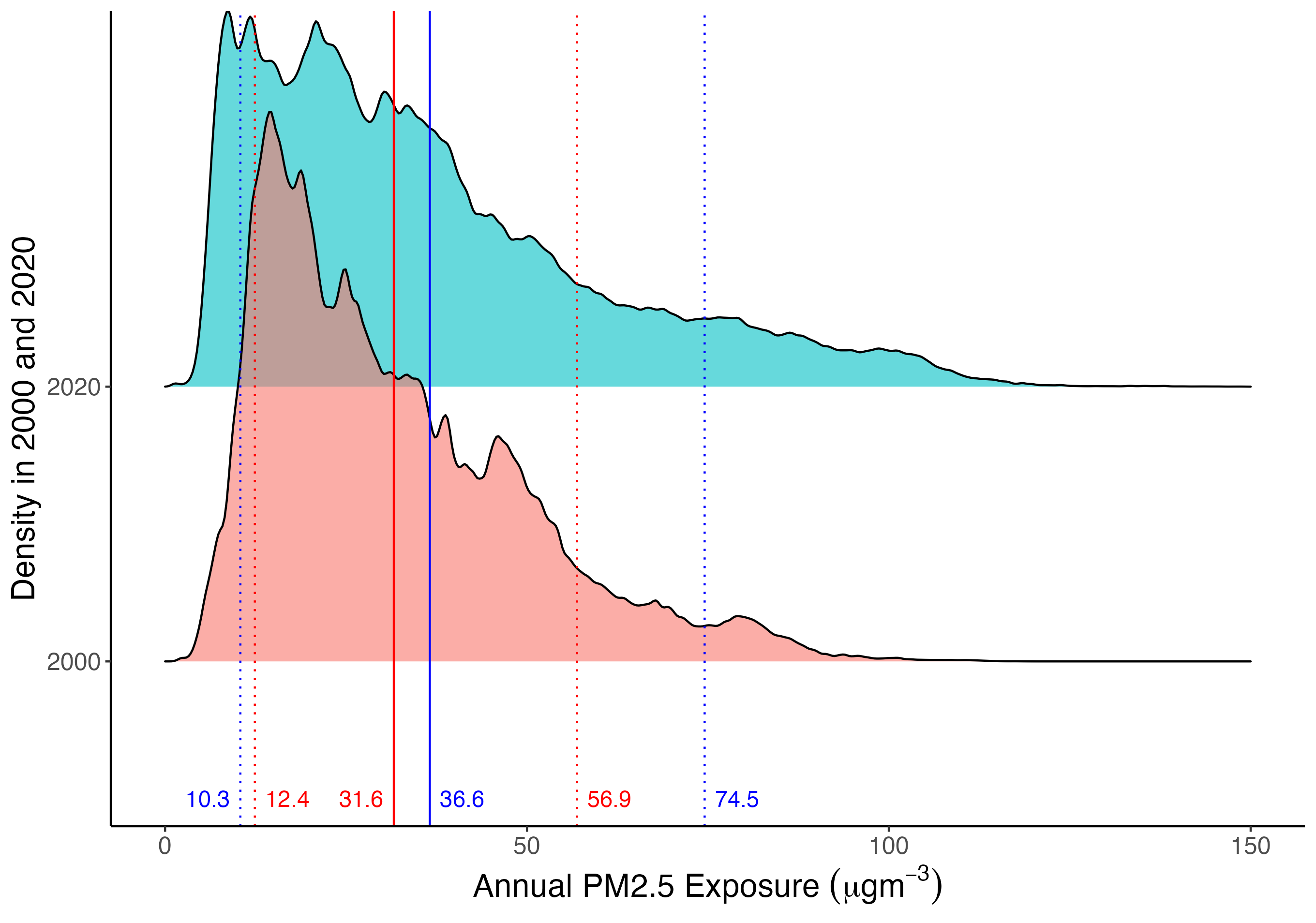
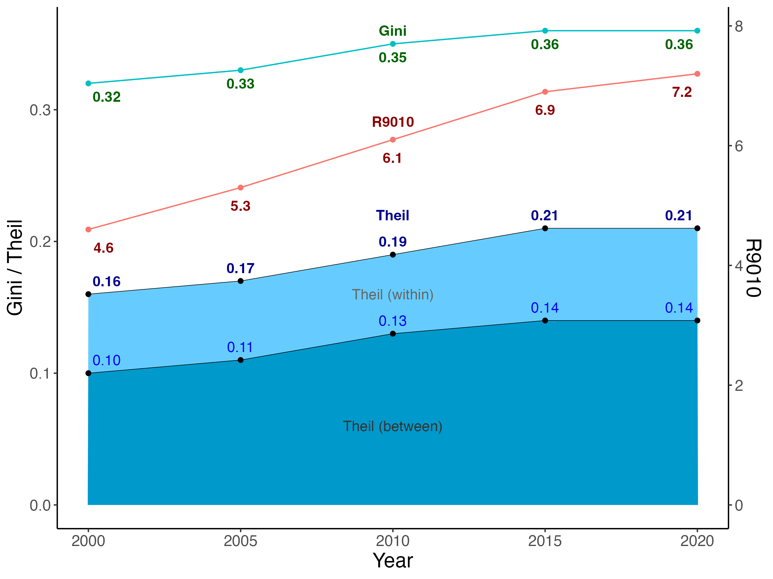
Figure 1: Global distribution of PM_2.5 exposure between 2000 and 2020. Left panel: Population-weighted Gaussian Kernel density estimates for PM_2.5 levels ($\mu gm^{-3}$) in 2000 and 2020, truncated at 150 $\mu gm^{-3}$. Solid lines indicate global mean PM_2.5 exposure and dashed lines are 10th and 90th percentiles. Right panel: Inequality indices for global PM_2.5 exposure 2000-2020 in 5-year intervals, measured as ratio of 90th to 10th percentile (R9010, right axis), Gini Index and Theil Index (left axis). Theil Index decomposition into between-country and within-country components following [27]. Population and pollution data from [15, 16].

Decomposition into differences between and within countries

The bulk of global air quality inequality can be attributed to differences between countries rather than variation within them. Using the Theil Index, which is exactly decomposable [27], in Figure 1 (right panel) we see that two thirds of global air quality inequality (0.14 out of 0.21) were due to differences between countries in 2020. Put differently, even if PM_2.5 exposure was fully equalized within every country in the world, two thirds of global air quality inequality would remain. Similar and even higher between-country contributions are shown by the other measures (Extended Data Table 1).

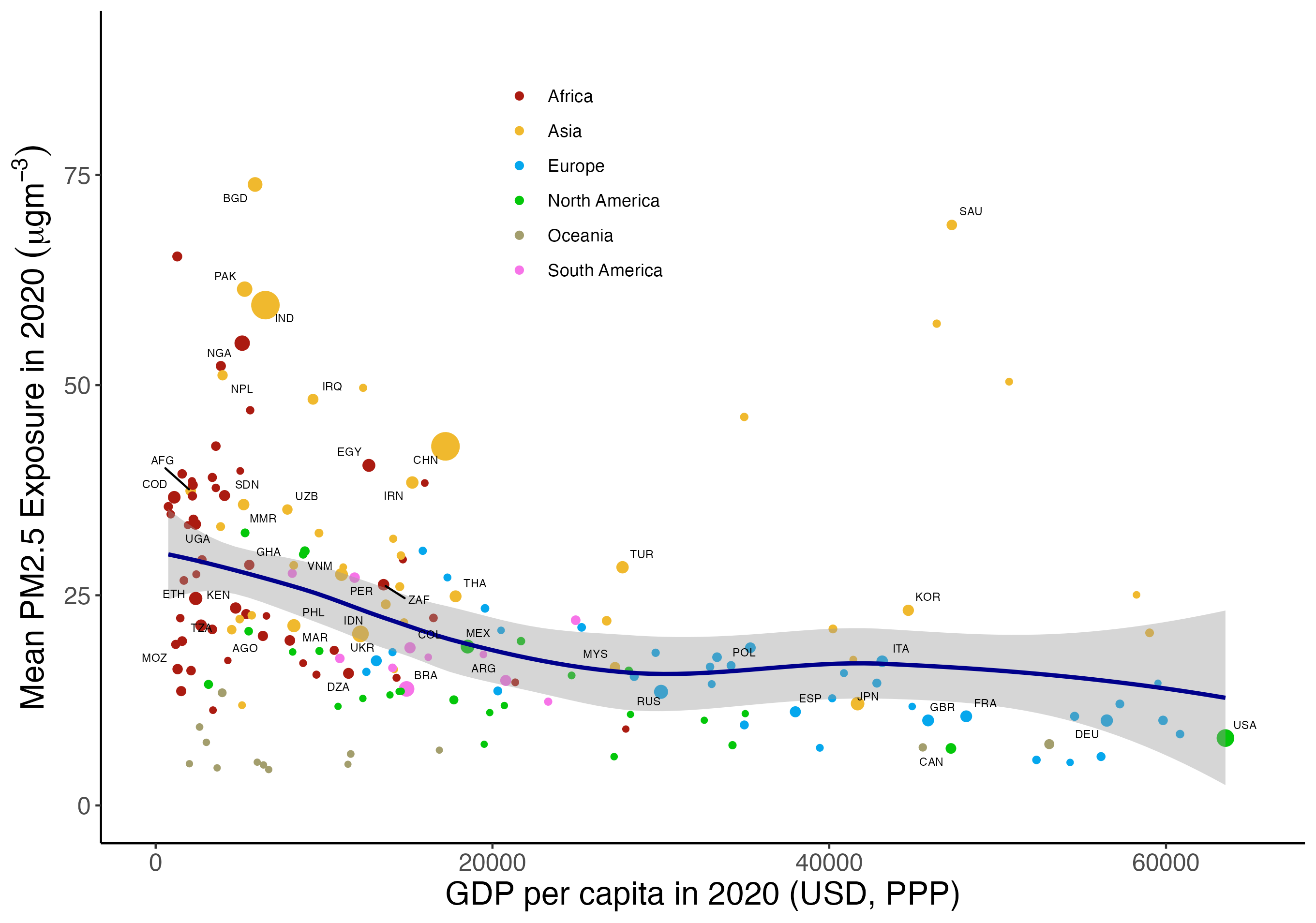
Figure 6: Country-level GDP per capita and mean PM_2.5 exposure in 2020. Population and pollution data from [15, 16]. Plot shows 191 out of 228 countries/regions with available GDP per capita in 2020 (current international dollars, PPP) from [30]. Circle size indicates population in 2020, color indicates continent. Line is fitted from a local polynomial regression with 95% confidence bands. Labels limited to the 50 countries with largest 2020 population.

Much of the increase in global air quality inequality is accounted for by rising differences between countries. The between-country portion of the Global PM_2.5 Theil Index rose from 0.10 to 0.14 between 2000 and 2020, while the within-country portion grew only slightly from 0.06 to 0.07. Another way to see this is in Figure 2, which shows divergence in country-level PM_2.5 exposure between 2000 and 2020 (left panel). Many countries with high PM_2.5 levels in 2000 had even higher levels in 2020. This is visible for South Asian countries such as India, Pakistan and Bangladesh, but also for China, Saudi Arabia and others. Meanwhile, many of the already less polluted countries in Europe and North America saw stagnating or even falling PM_2.5 levels. This reinforced a trend whereby PM_2.5 levels tend to be higher in low-income countries (Extended Data Figure 6), likely compounding global economic inequality [13, 14]. Meanwhile, within-country PM_2.5 inequality, measured by the Gini Index (right panel of Figure 2), increased in some countries but fell in others. Global PM_2.5 inequality is largely and increasingly driven by differences between countries.

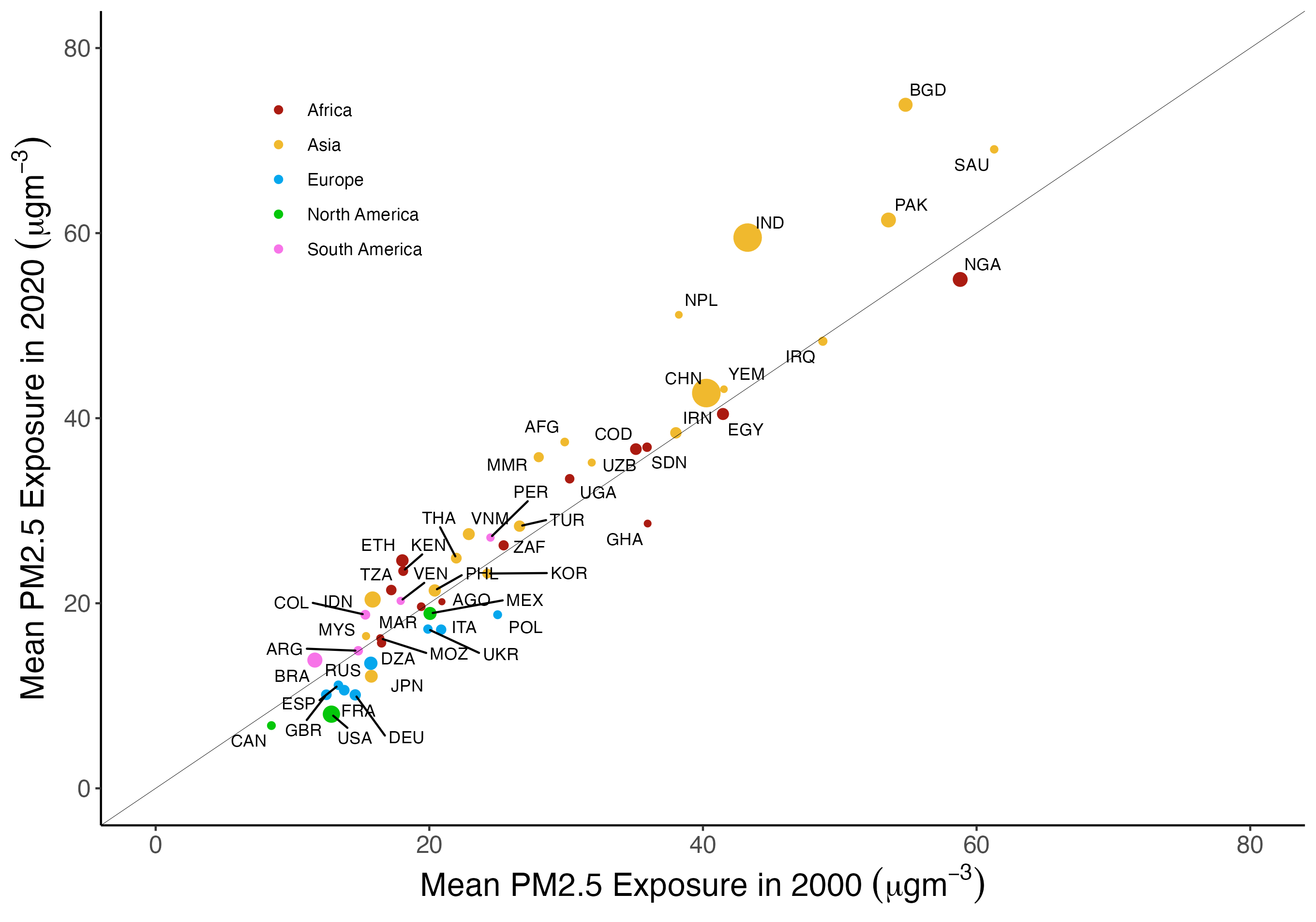
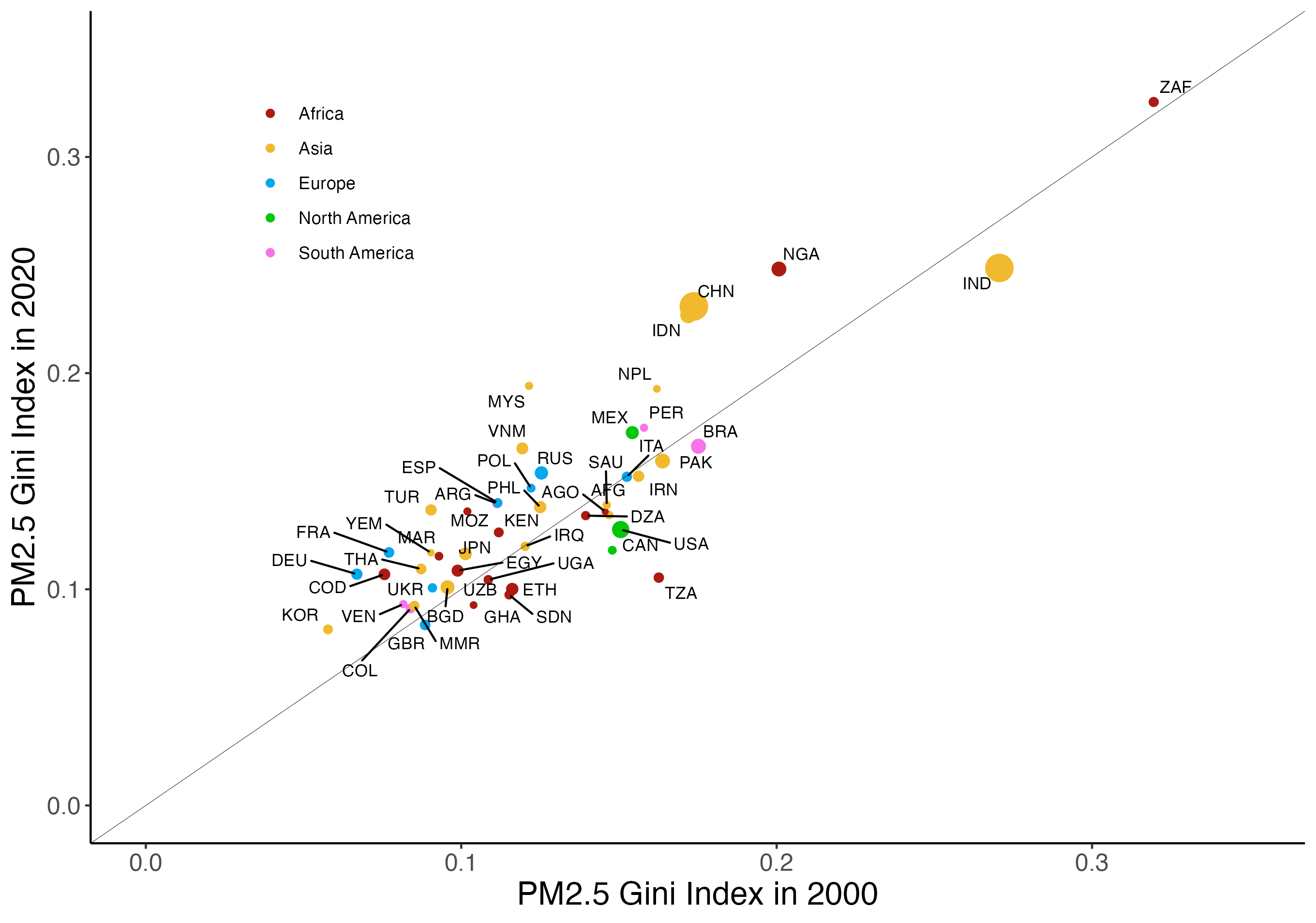
Figure 2: Country-level PM_2.5 exposure and inequality in 2000 and 2020. Left panel: Country-level population-weighted mean PM_2.5 exposure ($\mu gm^{-3}$) in 2000 and 2020. Right panel: Country-level Gini Index for PM_2.5 exposure in 2000 and 2020. Circle size indicates population in 2020, color indicates continent. Diagonal line represents equal levels in 2000 and 2020. Graph limited to the 50 countries with largest 2020 population. Population and pollution data from [15, 16].

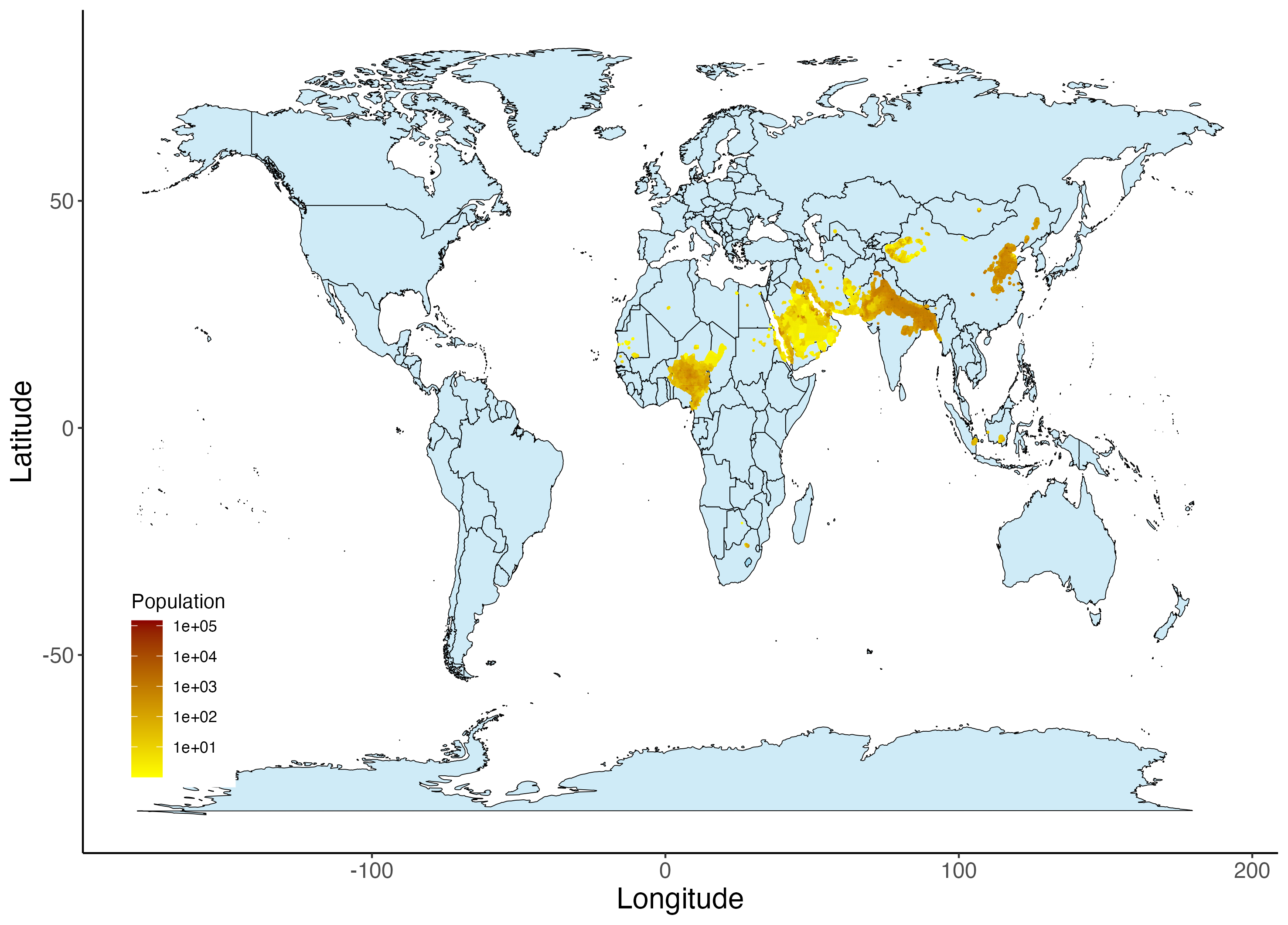
Figure 3: The ‘Choking Billion’. World map showing the location of the 1 billion people exposed to annual PM_2.5 over 63.6 $\mu gm^{-3}$ in 2020. Shading indicates population density. Population and pollution data from [15, 16].

‘Air Quality Poverty’ and the ‘Choking Billion’ High overall PM_2.5 exposure combined with pronounced inequality imply that a substantial portion of the world population faces very high levels of air pollution. Continuing the analogy with economic inequality, we can designate a group of the most exposed people as suffering from ‘air quality poverty’. Here, I focus on the 1 billion people facing the highest PM_2.5 exposure levels in 2020 (63.6 $\mu gm^{-3}$ or higher), which I call the ‘Choking Billion’. The map in Figure 3 shows that a few geographic clusters accounted for most of the ‘Choking Billion’ in 2020. The biggest cluster spans Northern India, Bangladesh, Pakistan and Nepal, followed by other big clusters in and around Eastern China, Northern Nigeria, and the Arab peninsula. India alone was home to over half (500 million) of the ‘Choking Billion’ in 2020, followed by China (155m), Bangladesh (127m) and Pakistan (93m), as detailed in Extended Data Table 2. Other countries also had high rates of air quality poverty. Notably, two thirds of the population of Saudi Arabia and most inhabitants of Qatar were part of the ‘Choking Billion’ in 2020, as were around half of people in Niger, and almost a third in Nigeria and Mongolia.

Discussion

The inequality indices calculated here document high and rising levels of global air quality inequality, as measured by annual ambient PM_2.5 exposure. The bulk of this inequality comes from differences between countries rather than variation within them. This suggests that research efforts and the public discourse on environmental justice, which tend to focus on air quality differences within countries [10, 11, 12], may overlook an important dimension of global environmental inequality.

Underlying rising mean exposure and exposure inequality is an increase at the upper tails of the PM_2.5 distribution. A large portion of those exposed to the highest levels of ambient PM_2.5 live in just a few countries in Asia and Africa. Much like economic poverty, ‘air quality poverty’ is geographically concentrated, often in places that also face economic hardship [13, 14]. Sustainable development initiatives, which increasingly recognize the importance of air quality improvements [4], may benefit from focusing on these pollution clusters.

The findings are subject to several limitations. Firstly, mismeasurement of either population counts or pollution levels may affect my results, which thus rely on the assumptions underlying the estimates in [15] and [16]. Secondly, the spatial resolution of 30 arc-seconds (500-900 meters depending on latitude) used here necessarily misses variation at smaller geographic scales. Finally, location-based measures of pollution concentrations are imprecise measures of actual exposure. Since PM_2.5 is measured in weight per volume ($\mu gm^{-3}$), assuming that all persons consume similar volumes of outdoor air, the indices capture inequality in total fine particles (by weight) inhaled. Effective exposure will differ based on additional factors, such as mobility patterns, building technology and time spent indoors[33].

Despite these limitations, the inequality indices calculated here offer a new, quantitative perspective on global air quality inequality. Similar indices may prove useful in describing other dimensions of environmental inequality. In particular, future research may test if air pollutants other than PM_2.5 are subject to similar inequality levels.

Author contributions L.S. conceived and conducted the research, analysed the results, wrote and reviewed the manuscript.

Declarations The author declares no competing interests.

Acknowledgments I thank Raphael Calel for helpful comments.

Methods

This article combines global gridded population counts with estimates of annual fine particulate matter (PM_2.5) concentrations to calculate inequality indices describing the global distribution of PM_2.5 exposure between 2000 and 2020.

Data Population count data are from Gridded Population of the World (GPW v4.11) [15], using UN WPP-adjusted population counts in 2000, 2005, 2010, 2015 and 2020 at a 30 arc-second (0.0083 degree) resolution. Data on PM_2.5 concentrations are from [16] (V5.GL.03), using estimates of annual mean surface-level PM_2.5 concentrations in 2000, 2005, 2010, 2015 and 2020 at a 0.01 arc-degree resolution.

Spatial matching The spatial unit of analysis are grid cells from GPW v4.11. In each year and for each population grid cell, PM_2.5 is assigned as follows: Where available, assign the PM_2.5 level at the pollution grid point closest (in arc-degrees) to the population grid point. When that PM_2.5 level is missing, use the mean of the non-missing values from the 8 next-closest grid points in arc-degree space (i.e. neighboring grid cells to the top-right, top, top-right, left, right, bottom-left, bottom, and bottom-right). This step extends my sample coverage, but does not substantially change the main results, as shown in SI Table 4.

Final sample Due to computational constraints, the analysis sample is limited as follows. First, all grid points with population estimates below 1 are dropped (this maintains 99.7% of the total population). Second, countries/territories with total populations below 10,000 in 2020 are dropped. In addition, the sample excludes grid cells that cannot be matched to a PM_2.5 estimate using the procedure described above. This results in a final sample of 80.1 million grid points in 228 countries/territories, accounting for 85% of the world population (Extended Data Figures 4 and 5)..

Inequality measures While economic inequality indices are usually applied to the distribution of income or wealth across individuals or households, I apply them to the distribution of ambient PM_2.5 across the world population. In a given year, each geographic grid cell ($i$) is matched to a PM_2.5 concentration ($P_{i}$). Population counts by grid cell ($n_{i}$) are used as weights to quantify pollution exposure across the world population ($N=\sum_{i}n_{i}$). Population-weighted global mean PM_2.5 exposure is $\overline{P}=\frac{1}{N}\sum_{i}n_{i}P_{i}$.

The inequality indices differ in the weight they place on different characteristics of the pollution exposure distribution. R9010 is calculated as the ratio of the 90th percentile of the population-weighted global PM_2.5 distribution divided by the 10th percentile. The Gini Index is defined as a ratio of weighted sums across grid cells $i,j$, so that $\text{Gini}=\frac{\sum_{i}n_{i}\sum_{j}n_{j}|P_{i}-P_{j}|}{2\overline{P}N^{2}}$.

The three remaining measures are members of the Generalized Entropy (GE) class of inequality indices with different values of the inequality aversion parameter $\alpha$. When $\alpha=0$, GE(0), also called the Mean Log Deviation (MLD), is defined as $GE(0)=\frac{1}{N}\sum_{i}\left[n_{i}log(\frac{\overline{P}}{P_{i}})\right]$. When $\alpha=1$, GE(1), also called the Theil Index, is defined as $GE(1)=\frac{1}{N}\sum_{i}\left[n_{i}\frac{P_{i}}{\overline{P}}log(\frac{P_{i}}{\overline{P}})\right]$. And when $\alpha=2$, GE(2), equal to half the square of the coefficient of variation, is defined as $GE(2)=\frac{1}{2}\left(\left[\sum_{i}\frac{n_{i}}{N}\frac{P_{i}}{\overline{P}}\right]^{2}-1\right)$.

All GE($\alpha$) measures are additively separable and can be decomposed into within-group and between-group inequality [18, 27], such that $GE(\alpha)=GE_{W}(\alpha)+GE_{B}(\alpha)$. Here, inequality within groups ($k$) is defined as $GE_{W}(\alpha)=\sum_{k}\left[(\frac{N_{k}}{N})\left(\frac{\overline{P}_{k}}{\overline{P}}\right)^{\alpha}GE_{k}(\alpha)\right]$ where $GE_{k}(\alpha)$ is calculated as standalone inequality measure for group $k$. Gini Index decomposition follows [28], but is not exhaustive when subgroup distributions overlap, resulting in an unexplained residual.

Extended Data

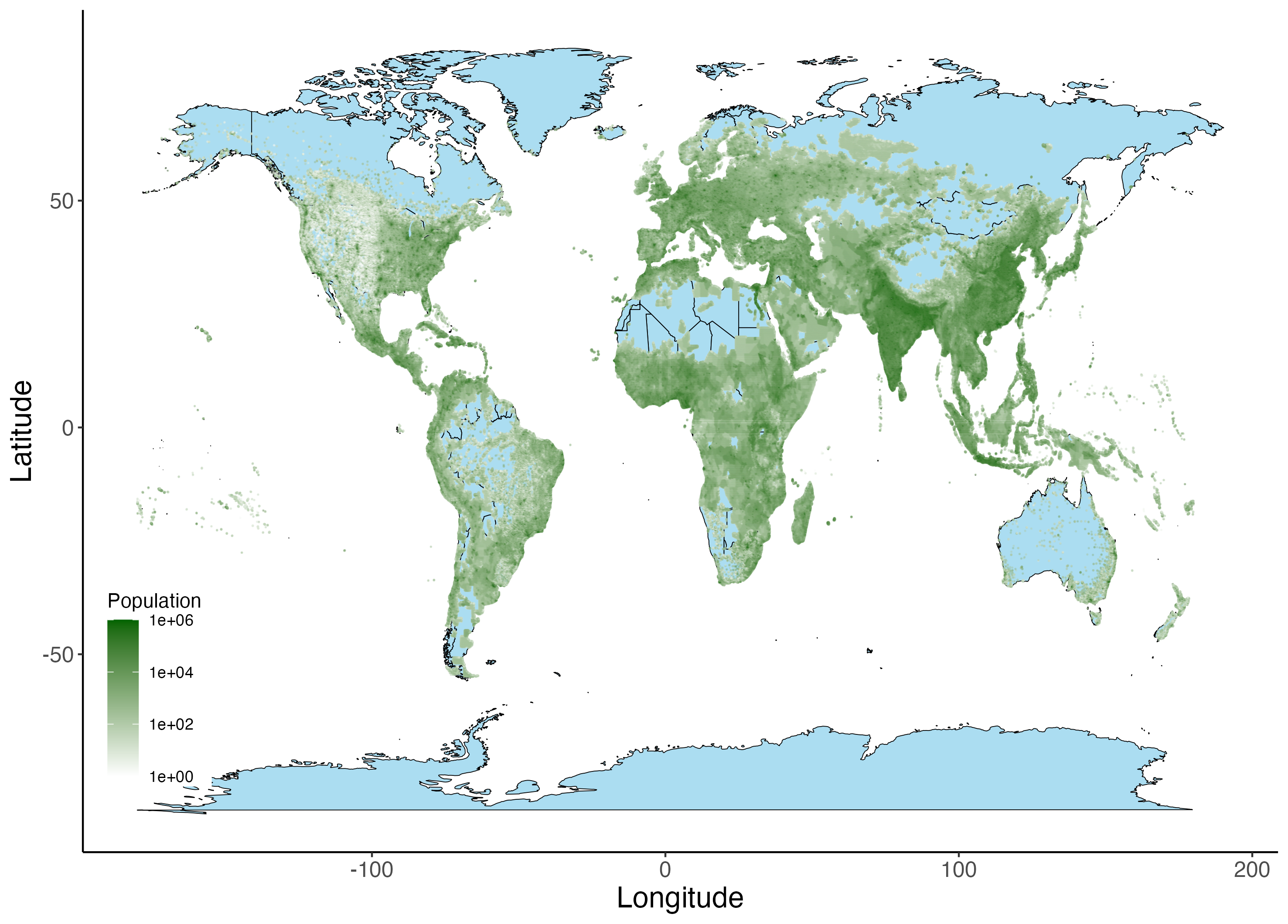
Figure 4: Population in 2020. Data from [15], limited to analysis sample.

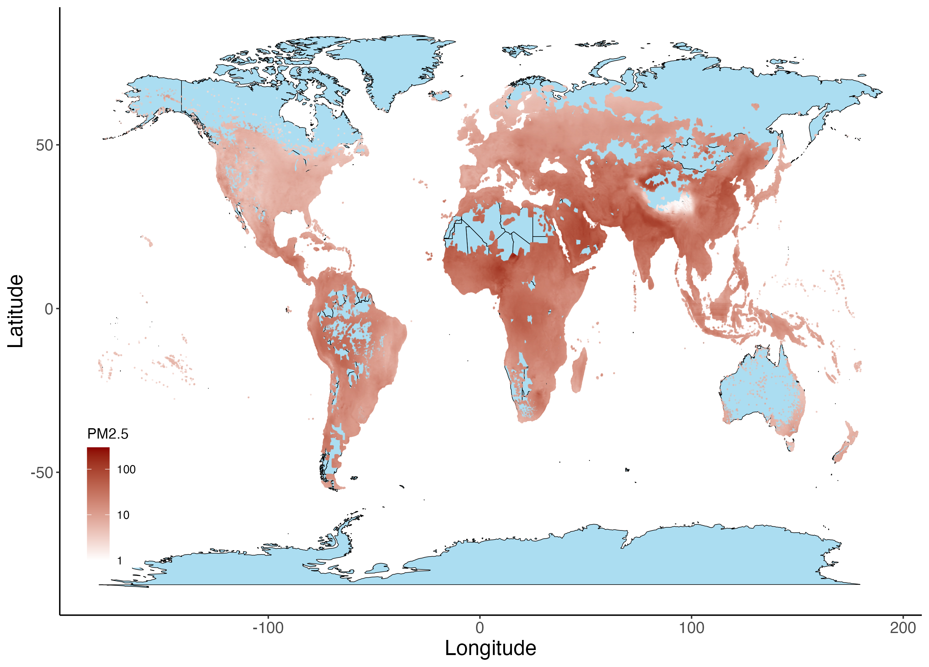
Figure 5: PM_2.5 concentrations in 2020. Data from [16], limited to analysis sample.

Table 1: Global PM_2.5 Exposure Inequality and Decomposition

	Mean	R9010	Gini	MLD	Theil	0.5CV2
2000	31.6	4.6	0.32	0.17	0.16	0.17
between			0.24	0.12	0.10	0.10
within			0.02	0.05	0.06	0.07
2010	38.1	6.1	0.35	0.21	0.19	0.20
between			0.27	0.16	0.13	0.12
within			0.03	0.05	0.06	0.08
2020	36.6	7.2	0.36	0.23	0.21	0.22
between			0.29	0.18	0.14	0.13
within			0.03	0.06	0.07	0.09

Table 2: The ‘Choking Billion’ by country

	‘Choking’	‘Choking’	Coverage	Total Pop.
	(million)	(in %)	(in %)	(million)
India	509.6	40	91	1262.0
China	154.8	12	92	1293.2
Bangladesh	127.2	79	94	160.4
Pakistan	92.7	48	93	193.5
Nigeria	46.2	29	76	158.0
Saudi Arabia	19.5	67	85	29.3
Nepal	8.7	30	95	28.7
Niger	6.9	46	61	14.9
Iran	4.2	6	82	68.5
Cameroon	3.0	18	64	16.9
Iraq	2.8	8	82	34.3
United Arab Emirates	2.1	26	86	8.4
Qatar	2.0	94	87	2.1
South Africa	0.9	2	94	53.2
Mongolia	0.7	31	69	2.2
Kuwait	0.5	14	83	3.6

Supplementary Information

Table 3: Data coverage by country or territory.

	ISO	Name of Country or Territory	Pop. in 2020	Coverage	PM2.5 in 2000	PM2.5 in 2020
			(thousands)	(%)	($\mu gm^{-3}$)	($\mu gm^{-3}$)
1	ABW	Aruba	105	46.3	10.7	10.9
2	AFG	Afghanistan	36452	89.0	29.9	37.4
3	AGO	Angola	29262	55.8	20.9	20.2
4	AIA	Anguilla	15	81.6	11.1	9.6
5	ALA	Åland Islands	30	91.4	6.7	4.9
6	ALB	Albania	2936	92.2	21.7	18.2
7	AND	Andorra	69	45.2	12.1	9.0
8	ARE	United Arab Emirates	9809	85.6	61.1	58.5
9	ARG	Argentina	45530	84.3	14.8	14.9
10	ARM	Armenia	3041	80.0	28.0	31.7
11	ASM	American Samoa	56	91.2	3.8	4.3
12	ATG	Antigua and Barbuda	96	79.8	13.0	11.0
13	AUS	Australia	25595	90.1	5.8	7.3
14	AUT	Austria	8660	71.7	16.7	12.1
15	AZE	Azerbaijan	10232	80.4	27.8	26.0
16	BDI	Burundi	13106	69.1	33.6	35.5
17	BEL	Belgium	11641	90.7	14.2	10.6
18	BEN	Benin	12355	77.9	43.1	39.0
19	BES	Bonaire Saint Eustatius and Saba	26	76.1	12.2	11.5
20	BFA	Burkina Faso	20865	60.5	40.7	38.1
21	BGD	Bangladesh	170397	94.1	54.8	73.9
22	BGR	Bulgaria	6909	89.7	27.7	21.2
23	BHR	Bahrain	1486	88.3	52.4	50.4
24	BHS	Bahamas	410	88.8	7.7	5.8
25	BIH	Bosnia and Herzegovina	3757	89.9	30.3	30.3
26	BLR	Belarus	9362	90.2	17.0	13.6
27	BLZ	Belize	398	93.7	17.1	18.3
28	BMU	Bermuda	61	94.0	7.1	5.6
29	BOL	Bolivia (Plurinational State of)	11550	87.2	23.4	27.6
30	BRA	Brazil	215984	76.0	11.6	13.9
31	BRB	Barbados	288	59.9	14.4	13.6
32	BRN	Brunei Darussalam	450	76.9	5.7	8.3
33	BTN	Bhutan	834	94.2	23.5	28.3
34	BWA	Botswana	2458	87.2	14.9	15.2
35	CAF	Central African Republic	5399	79.2	36.3	34.6
36	CAN	Canada	37599	87.9	8.5	6.8
37	CHE	Switzerland	8653	74.2	14.2	10.6
38	CHL	Chile	18841	89.0	19.5	22.0
39	CHN	China	1402773	92.2	40.2	42.7
40	CIV	Côte d’Ivoire	25566	93.5	23.6	22.8
41	CMR	Cameroon	26350	64.0	56.7	52.3
42	COD	Democratic Republic of the Congo	90176	75.4	35.1	36.7
43	COG	Congo	5262	66.5	28.0	37.8
44	COK	Cook Islands	21	98.6	3.9	4.2
45	COL	Colombia	50230	73.2	15.3	18.8
46	COM	Comoros	883	66.0	10.6	11.3
47	CPV	Cape Verde	553	84.1	28.9	22.5
48	CRI	Costa Rica	5045	71.7	16.5	19.5
49	CUB	Cuba	11366	93.5	11.5	10.4
50	CUW	Curaçao	164	73.6	11.5	11.9
51	CYM	Cayman Islands	64	98.2	10.9	11.1
52	CYP	Cyprus	1218	80.3	20.3	17.3
53	CZE	Czech Republic	10576	73.0	20.7	14.6
54	DEU	Germany	80389	69.9	14.6	10.1
55	DJI	Djibouti	946	66.8	39.4	39.8
56	DMA	Dominica	74	61.5	11.7	11.8
57	DNK	Denmark	5776	61.0	13.1	8.5
58	DOM	Dominican Republic	11112	95.1	11.8	12.6
59	DZA	Algeria	43007	82.7	16.5	15.7
60	ECU	Ecuador	17340	70.3	14.0	17.5
61	EGY	Egypt	100524	94.0	41.5	40.5
62	ERI	Eritrea	5893	68.9	32.5	32.7
63	ESH	Western Sahara	634	70.2	35.6	29.7
64	ESP	Spain	46178	84.2	13.4	11.1
65	EST	Estonia	1293	88.7	8.8	6.9
66	ETH	Ethiopia	111983	65.3	18.0	24.6
67	FIN	Finland	5555	86.8	6.9	5.4
68	FJI	Fiji	915	98.9	6.5	6.1
69	FRA	France	65734	84.2	13.8	10.6
70	FRO	Faeroe Islands	49	90.0	5.2	5.4
71	FSM	Micronesia (Federated States of)	108	83.9	4.2	4.5
72	GAB	Gabon	1919	56.7	23.8	29.3
73	GBR	United Kingdom	66699	78.8	12.5	10.1
74	GEO	Georgia	3980	80.0	20.0	21.8
75	GGY	Guernsey	63	78.0	10.4	8.9
76	GHA	Ghana	30548	79.8	36.0	28.6
77	GIB	Gibraltar	34	84.0	13.3	13.0
78	GIN	Guinea	14354	50.9	31.6	29.2
79	GLP	Guadeloupe	419	81.5	11.6	11.6
80	GMB	Gambia	2319	63.0	47.6	38.6
81	GNB	Guinea-Bissau	2070	52.9	39.9	33.3
82	GNQ	Equatorial Guinea	970	53.5	35.6	38.4
83	GRC	Greece	10828	87.9	19.6	15.3
84	GRD	Grenada	109	64.6	14.4	13.1
85	GRL	Greenland	56	60.4	2.1	1.7
86	GTM	Guatemala	18015	71.6	31.2	30.3
87	GUF	French Guiana	305	63.8	14.6	16.0
88	GUM	Guam	180	64.7	3.2	4.4
89	GUY	Guyana	787	70.0	17.2	18.0
90	HKG	Hong Kong	7619	89.9	25.6	20.5
91	HND	Honduras	8656	68.9	28.6	32.4
92	HRV	Croatia	4164	80.5	21.2	18.2
93	HTI	Haiti	11373	93.9	12.7	14.4
94	HUN	Hungary	9684	89.6	23.0	16.6
95	IDN	Indonesia	271854	76.1	15.9	20.4
96	IMN	Isle of Man	91	78.5	8.6	8.1
97	IND	India	1388953	90.9	43.3	59.5
98	IRL	Ireland	4875	81.2	9.4	8.1
99	IRN	Iran (Islamic Republic of)	83401	82.1	38.0	38.4
100	IRQ	Iraq	41963	81.7	48.8	48.3
101	ISL	Iceland	342	81.3	5.2	5.1
102	ISR	Israel	8733	83.5	20.1	21.0
103	ITA	Italy	59743	66.3	20.9	17.2
104	JAM	Jamaica	2840	93.9	16.7	18.4
105	JEY	Jersey	105	88.9	10.8	9.3
106	JOR	Jordan	8167	83.9	28.1	32.4
107	JPN	Japan	125039	89.7	15.8	12.1
108	KAZ	Kazakhstan	18626	82.0	17.3	22.0
109	KEN	Kenya	52175	71.3	18.1	23.5
110	KGZ	Kyrgyzstan	6426	91.2	22.2	22.2
111	KHM	Cambodia	16809	67.4	18.5	20.9
112	KIR	Kiribati	122	39.8	4.3	5.0
113	KNA	Saint Kitts and Nevis	58	80.3	12.6	10.8
114	KOR	Republic of Korea	51252	89.6	24.2	23.2
115	KWT	Kuwait	4314	83.0	59.6	57.3
116	LAO	Lao People’s Democratic Republic	7407	89.8	23.2	28.6
117	LBN	Lebanon	5897	84.4	28.4	29.7
118	LBR	Liberia	5093	69.3	20.1	22.3
119	LBY	Libya	6700	67.8	26.2	22.3
120	LCA	Saint Lucia	192	62.8	13.8	12.7
121	LIE	Liechtenstein	39	47.5	14.2	10.5
122	LKA	Sri Lanka	21157	76.7	19.6	23.9
123	LSO	Lesotho	2241	95.9	24.6	27.5
124	LTU	Lithuania	2795	89.2	15.6	12.7
125	LUX	Luxembourg	599	92.3	13.3	9.8
126	LVA	Latvia	1920	88.2	17.5	14.4
127	MAC	Macau	632	99.9	29.5	25.1
128	MAF	Saint-Martin (French part)	46	69.8	10.7	9.3
129	MAR	Morocco	36457	85.7	19.4	19.6
130	MCO	Monaco	26	75.9	16.7	12.5
131	MDA	Republic of Moldova	4015	91.1	18.2	15.9
132	MDG	Madagascar	27799	82.9	11.3	13.6
133	MDV	Maldives	393	56.8	15.3	16.2
134	MEX	Mexico	134787	93.7	20.1	18.9
135	MHL	Marshall Islands	53	78.0	4.3	5.1
136	MKD	Macedonia	2087	90.0	32.3	27.1
137	MLI	Mali	20458	65.2	38.7	34.0
138	MLT	Malta	423	64.2	13.0	11.8
139	MMR	Myanmar	56256	93.1	28.0	35.8
140	MNE	Montenegro	626	90.1	21.2	20.8
141	MNG	Mongolia	3180	68.9	32.2	49.7
142	MNP	Northern Mariana Islands	56	91.6	2.9	3.4
143	MOZ	Mozambique	32025	75.6	16.4	16.2
144	MRT	Mauritania	4569	63.1	55.1	47.0
145	MTQ	Martinique	395	62.9	16.7	16.3
146	MUS	Mauritius	1291	80.9	15.5	14.6
147	MWI	Malawi	19993	65.6	16.4	19.6
148	MYS	Malaysia	32374	68.0	15.4	16.5
149	MYT	Mayotte	273	62.7	12.3	13.0
150	NAM	Namibia	2722	77.4	15.6	15.6
151	NCL	New Caledonia	280	98.1	6.3	6.2
152	NER	Niger	24316	61.4	66.4	65.3
153	NGA	Nigeria	206824	76.4	58.8	55.0
154	NIC	Nicaragua	6416	70.5	18.2	20.7
155	NLD	Netherlands	17184	89.9	14.8	10.1
156	NOR	Norway	5490	65.2	8.1	5.7
157	NPL	Nepal	30197	95.1	38.2	51.2
158	NRU	Nauru	10	100.0	4.6	4.9
159	NZL	New Zealand	4730	88.8	6.3	6.9
160	OMN	Oman	4826	85.1	47.6	46.2
161	PAK	Pakistan	208366	92.9	53.6	61.4
162	PAN	Panama	4230	69.4	13.7	16.0
163	PER	Peru	33317	72.6	24.5	27.1
164	PHL	Philippines	108436	72.7	20.4	21.4
165	PLW	Palau	22	90.3	6.6	6.6
166	PNG	Papua New Guinea	8413	89.1	9.7	13.4
167	POL	Poland	38409	88.3	25.0	18.8
168	PRI	Puerto Rico	3675	94.8	8.1	7.2
169	PRK	Democratic People’s Republic of Korea	25760	89.8	23.8	25.6
170	PRT	Portugal	10163	67.1	11.7	9.6
171	PRY	Paraguay	7064	84.8	14.0	16.4
172	PSE	State of Palestine	5317	83.9	21.2	22.6
173	PYF	French Polynesia	296	97.0	4.5	4.8
174	QAT	Qatar	2452	87.1	76.5	87.0
175	REU	Réunion	892	83.4	6.6	6.1
176	ROU	Romania	18829	88.4	20.9	17.6
177	RUS	Russian Federation	142900	80.3	15.7	13.5
178	RWA	Rwanda	13013	53.9	36.4	36.8
179	SAU	Saudi Arabia	34371	85.1	61.3	69.1
180	SDN	Sudan	45307	70.2	35.9	36.9
181	SEN	Senegal	17493	59.8	49.1	42.7
182	SGP	Singapore	6007	44.8	17.3	16.5
183	SLB	Solomon Islands	640	78.1	6.5	9.3
184	SLE	Sierra Leone	7160	55.1	26.1	26.8
185	SLV	El Salvador	6227	70.1	28.8	29.9
186	SMR	San Marino	31	58.2	17.8	14.5
187	SOM	Somalia	12436	62.3	20.2	19.2
188	SRB	Serbia	6645	90.2	23.0	23.4
189	SSD	South Sudan	14116	71.9	22.7	22.2
190	STP	Sao Tome and Principe	211	97.5	20.7	17.2
191	SUR	Suriname	565	74.9	17.1	17.6
192	SVK	Slovakia	5434	89.3	22.3	16.5
193	SVN	Slovenia	2077	65.1	20.2	15.7
194	SWE	Sweden	10121	74.5	8.4	5.8
195	SWZ	Swaziland	1366	95.8	21.5	16.9
196	SXM	Sint Maarten (Dutch part)	42	83.1	11.1	10.1
197	SYC	Seychelles	99	67.6	9.2	9.1
198	SYR	Syrian Arab Republic	20987	81.2	29.7	32.6
199	TCA	Turks and Caicos Islands	37	94.0	9.3	7.3
200	TCD	Chad	16422	61.6	40.3	39.4
201	TGO	Togo	8273	63.5	43.4	33.5
202	THA	Thailand	68596	76.4	22.0	24.9
203	TJK	Tajikistan	9416	91.0	25.5	33.2
204	TKM	Turkmenistan	5702	80.0	36.7	31.3
205	TLS	Timor-Leste	1317	64.7	11.1	11.9
206	TON	Tonga	111	99.1	4.8	4.3
207	TTO	Trinidad and Tobago	1378	61.0	15.4	15.5
208	TUN	Tunisia	11836	62.2	23.0	18.5
209	TUR	Turkey	82262	86.1	26.6	28.3
210	TWN	Taiwan	23402	93.5	24.2	19.8
211	TZA	United Republic of Tanzania	62280	65.4	17.2	21.4
212	UGA	Uganda	45836	73.8	30.3	33.5
213	UKR	Ukraine	43678	85.5	19.9	17.2
214	URY	Uruguay	3492	82.1	12.0	12.3
215	USA	United States of America	333422	90.3	12.8	8.0
216	UZB	Uzbekistan	31709	88.4	31.9	35.2
217	VCT	Saint Vincent and the Grenadines	111	76.2	14.3	13.6
218	VEN	Venezuela (Bolivarian Republic of)	33118	69.0	17.9	20.3
219	VGB	British Virgin Islands	33	94.6	7.7	7.2
220	VIR	United States Virgin Islands	107	91.8	7.0	6.5
221	VNM	Viet Nam	98139	80.5	22.9	27.5
222	VUT	Vanuatu	294	87.7	7.5	7.5
223	WLF	Wallis and Futuna Islands	13	77.8	4.4	4.7
224	WSM	Western Samoa	199	70.8	4.5	4.8
225	YEM	Yemen	30029	63.9	41.5	43.1
226	ZAF	South Africa	56689	93.9	25.4	26.3
227	ZMB	Zambia	18889	72.3	18.5	20.9
228	ZWE	Zimbabwe	17464	93.8	15.3	16.0
Source: The 228 countries or territories in the sample, sorted by 2020 population. Names and population estimates from [15].
‘Coverage’ shows ratio of country population in sample to total country population.
‘PM2.5 in 2000/2020’ are population-weighted mean exposure levels in 2000 and 2020 respectively, based on [16].

Table 4: Replication of Table 1 (sample restricted to nearest neighbor PM_2.5)

	Mean	R9010	Gini	MLD	Theil	0.5CV2
2000	31.10	4.60	0.32	0.17	0.16	0.17
between			0.25	0.12	0.11	0.10
within			0.02	0.05	0.06	0.07
2010	37.30	6.00	0.35	0.21	0.19	0.20
between			0.28	0.16	0.13	0.12
within			0.02	0.05	0.06	0.08
2020	34.10	7.20	0.37	0.24	0.22	0.24
between			0.31	0.18	0.16	0.16
within			0.02	0.05	0.06	0.09

References

- \bibcommenthead
- [1] Landrigan, P. J. et al. The lancet commission on pollution and health. The Lancet 391, 462–512 (2018).
- [2] Murray, C. J. et al. Global burden of 87 risk factors in 204 countries and territories, 1990–2019: a systematic analysis for the global burden of disease study 2019. The Lancet 396, 1223–1249 (2020).
- [3] Aguilar-Gomez, S., Dwyer, H., Graff Zivin, J. & Neidell, M. This is air: The “nonhealth” effects of air pollution. Annual Review of Resource Economics 14, 403–425 (2022).
- [4] Sachs, J. D. et al. Six transformations to achieve the sustainable development goals. Nature Sustainability 2, 805–814 (2019).
- [5] Southerland, V. A. et al. Global urban temporal trends in fine particulate matter (pm2.5) and attributable health burdens: estimates from global datasets. The Lancet Planetary Health 6, e139–e146 (2022).
- [6] Sicard, P. et al. Trends in urban air pollution over the last two decades: A global perspective. Science of The Total Environment 858, 160064 (2023).
- [7] Hajat, A., Hsia, C. & O’Neill, M. S. Socioeconomic disparities and air pollution exposure: a global review. Current Environmental Health Reports 2, 440–450 (2015).
- [8] Jbaily, A. et al. Air pollution exposure disparities across us population and income groups. Nature 601, 228–233 (2022).
- [9] Currie, J., Voorheis, J. & Walker, R. What caused racial disparities in particulate exposure to fall? new evidence from the clean air act and satellite-based measures of air quality. American Economic Review 113, 71–97 (2023).
- [10] Mohai, P., Pellow, D. & Roberts, J. T. Environmental justice. Annual Review of Environment and Resources 34, 405–430 (2009).
- [11] Banzhaf, S., Ma, L. & Timmins, C. Environmental justice: The economics of race, place, and pollution. Journal of Economic Perspectives 33, 185–208 (2019).
- [12] Drupp, M. A., Kornek, U., Meya, J. & Sager, L. Inequality and the environment: The economics of a two-headed hydra. Preprint at https://www.cesifo.org/DocDL/cesifo1_wp9447.pdf (2021).
- [13] Apte, J. et al. Air inequality: global divergence in urban fine particulate matter trends. Preprint at https://doi.org/10.26434/chemrxiv.14671908.v1 (2021).
- [14] Rentschler, J. & Leonova, N. Global air pollution exposure and poverty. Nature Communications 14, 4432 (2023).
- [15] CIESIN. Gridded Population of the World, Version 4 (GPWv4): Population Count Adjusted to Match 2015 Revision of UN WPP Country Totals Revision 11 (NASA Socioeconomic Data and Applications Center (SEDAC), 2018). Data accessed on 9 March 2023.
- [16] Van Donkelaar, A. et al. Monthly global estimates of fine particulate matter and their uncertainty. Environmental Science & Technology 55, 15287–15300 (2021). Data accessed on 7 March 2023.
- [17] Gini, C. Measurement of inequality of incomes. The Economic Journal 31, 124–125 (1921).
- [18] Shorrocks, A. F. The class of additively decomposable inequality measures. Econometrica 613–625 (1980).
- [19] Clark, L. P., Millet, D. B. & Marshall, J. D. National patterns in environmental injustice and inequality: outdoor no2 air pollution in the united states. PloS one 9, e94431 (2014).
- [20] Boyce, J. K., Zwickl, K. & Ash, M. Measuring environmental inequality. Ecological Economics 124, 114–123 (2016).
- [21] Rosofsky, A., Levy, J. I., Zanobetti, A., Janulewicz, P. & Fabian, M. P. Temporal trends in air pollution exposure inequality in massachusetts. Environmental Research 161, 76–86 (2018).
- [22] Pisoni, E., Dominguez-Torreiro, M. & Thunis, P. Inequality in exposure to air pollutants: A new perspective. Environmental Research 212, 113358 (2022).
- [23] Levy, J. I., Wilson, A. M. & Zwack, L. M. Quantifying the efficiency and equity implications of power plant air pollution control strategies in the united states. Environmental Health Perspectives 115, 743–750 (2007).
- [24] Fann, N. et al. Maximizing health benefits and minimizing inequality: incorporating local-scale data in the design and evaluation of air quality policies. Risk Analysis: An International Journal 31, 908–922 (2011).
- [25] Holland, S. P., Mansur, E. T., Muller, N. Z. & Yates, A. J. Distributional effects of air pollution from electric vehicle adoption. Journal of the Association of Environmental and Resource Economists 6, S65–S94 (2019).
- [26] Mansur, E. T. & Sheriff, G. On the measurement of environmental inequality: ranking emissions distributions generated by different policy instruments. Journal of the Association of Environmental and Resource Economists 8, 721–758 (2021).
- [27] Shorrocks, A. F. Inequality decomposition by population subgroups. Econometrica 1369–1385 (1984).
- [28] Mookherjee, D. & Shorrocks, A. A decomposition analysis of the trend in uk income inequality. The Economic Journal 92, 886–902 (1982).
- [29] WHO. WHO global air quality guidelines: particulate matter (PM2. 5 and PM10), ozone, nitrogen dioxide, sulfur dioxide and carbon monoxide: executive summary (World Health Organization, Geneva, 2021).
- [30] World Bank. World development indicators (2019). SI.POV.GINI and NY.GDP.PCAP.PP.CD accessed on 10 March 2023.
- [31] Chancel, L. Global carbon inequality over 1990–2019. Nature Sustainability 5, 931–938 (2022).
- [32] Collier, P. The Bottom Billion: Why the poorest countries are failing and what can be done about it (Oxford University Press, USA, 2008).
- [33] Jones, A. P. Indoor air quality and health. Atmospheric Environment 33, 4535–4564 (1999).