Resonance-aware NLOPS matching for off-shell $t\bar{t}+tW$ production with semileptonic decays

Abstract

The increasingly high accuracy of top-quark studies at the LHC calls for a theoretical description of $t\bar{t}$ production and decay in terms of exact matrix elements for the full $2\to 6$ process that includes the off-shell production and the chain decays of $t\bar{t}$ and $tW$ intermediate states, together with their quantum interference. Corresponding NLO QCD calculations matched to parton showers are available for the case of dileptonic channels and are implemented in the bb4l Monte Carlo generator, which is based on the resonance-aware POWHEG method. In this paper, we present the first NLOPS predictions of this kind for the case of semileptonic channels. In this context, the interplay of off-shell $t\bar{t}+tW$ production with various other QCD and electroweak subprocesses that yield the same semileptonic final state is discussed in detail. On the technical side, we improve the resonance-aware POWHEG procedure by means of new resonance histories based on matrix elements, which enable a realistic separation of $t\bar{t}$ and $tW$ contributions. Moreover, we introduce a general approach which makes it possible to avoid certain spurious terms that arise from the perturbative expansion of decay widths in any off-shell higher-order calculation, and which are large enough to jeopardise physical finite-width effects. These methods are implemented in a new version of the bb4l Monte Carlo generator, which is applicable to all dileptonic and semileptonic channels, and can be extended to fully hadronic channels. The presented results include a NLOPS comparison of off-shell against on-shell $t\bar{t}+tW$ production and decay, where we highlight various non-trivial aspects related to NLO and parton-shower radiation in leptonic and hadronic top decays.

1 Introduction

Studies of top-quarks play a key role in the ongoing physics programme of the Large Hadron Collider (LHC). Measurements in the different top-quark production modes, and especially in the ubiquitous $t\bar{t}$ production mode, allow for a detailed exploration of top-quark interactions, and a precise determination of fundamental Standard Model (SM) properties such as the top-quark mass. At the same time, top-quark–pair production represents a sizeable and challenging background for countless measurements and searches at the LHC. The sensitivity of such analyses critically relies on the precision of theoretical predictions for the $t\bar{t}$ production cross section, as well as for a large variety of kinematic distributions depending on the details of the nontrivial signatures that result from $t\bar{t}$ production and decay. This calls for the highest possible accuracy in the theoretical description of the production of top-quark pairs and their decays. In fact, the expected sensitivity of future experimental analyses requires precise theoretical predictions at the level of the full $2\to 6$ processes that correspond to $t\bar{t}$ production with dileptonic, semileptonic or fully hadronic decays, including all relevant off-shell effects, irreducible backgrounds and interferences. Such theoretical predictions provide a unified description of off-shell $t\bar{t}$ and $tW$ single-top production, including $t\bar{t}$–$tW$ interference effects Cascioli:2013wga ; Jezo:2016ujg .

For the analysis of experimental data, theoretical calculations need to be matched to parton showers. Monte Carlo generators that match NLO QCD calculations of on-shell $t\bar{t}$ production to parton showers are well established Frixione:2003ei ; Frixione:2007nw ; Alwall:2014hca ; Hoeche:2014qda ; Cormier:2018tog . Such tools describe top-quark decays based on spin-correlated LO matrix elements Frixione:2007zp ; Artoisenet:2012st ; Garzelli:2014dka ; Hoche:2014kca and implement a naive modelling of off-shell effects according to Breit–Wigner distributions. The emission of QCD radiation within top decays is controlled by the parton shower Sjostrand:2007gs ; Sjostrand:2014zea , which can dispose of built-in matrix-element corrections that provide a decent approximation of NLO effects. In the following, tools of this kind are going to be referred to as on-shell generators. The first generator that matches NNLO QCD calculations  Czakon:2013goa ; Czakon:2015owf ; Catani:2019iny ; Catani:2019hip of on-shell $t\bar{t}$ production to parton showers was presented in Mazzitelli:2021mmm ; Mazzitelli:2020jio .

A generator based on NLO QCD calculations where $t\bar{t}$ production and decay are both described at NLO in the narrow-width approximation (NWA) Bernreuther:2004jv ; Melnikov:2009dn ; Campbell:2012uf was presented in Campbell:2014kua . Corresponding NNLO QCD implementations of the NWA are also available, but only at fixed order Gao:2012ja ; Brucherseifer:2013iv ; Gao:2017goi ; Behring:2019iiv ; Czakon:2020qbd .

Concerning $tW$ single-top production, on-shell NLOPS generators are available in the five-flavour number scheme (5FNS) Re:2010bp ; Frixione:2008yi ; Bothmann:2017jfv . In this scheme, the NLO QCD corrections involve partonic channels of type $gg\to tW^{-}\bar{b}$, which entail resonant $t\bar{t}$ topologies that can lead to a double counting of the $t\bar{t}$ LO cross section. This issue can be avoided through various methods for the systematic separation of $tW$ from $t\bar{t}$ production Zhu:2001hw ; Campbell:2005bb ; Frixione:2008yi ; White:2009yt ; Demartin:2016axk . However, such methods are always subject to a degree of arbitrariness that is either due to ad-hoc prescriptions, violations of gauge invariance, or to the treatment of interference and off-shell effects.

A fully consistent solution of such issues is provided by calculations where the production and decays of $t\bar{t}$ pairs are described in terms of exact matrix elements for the corresponding $2\to 6$ process, without relying on the NWA. In this approach, using the complex-mass scheme Denner:2005fg , all possible $2\to 6$ topologies that involve off-shell $t\bar{t}$ and $tW$ intermediate states are handled on the same footing as contributions to subtopologies with off-shell $W^{+}W^{-}b\bar{b}$ states. Corresponding NLO calculations in the 5FNS are available at NLO QCD for dileptonic Bevilacqua:2010qb ; Denner:2010jp ; Denner:2012yc ; Heinrich:2013qaa ; Frederix:2013gra ; Cascioli:2013wga as well as for semileptonic Denner:2017kzu processes. When performed in the four-flavour number scheme (4FSN), i.e. treating $b$-quarks as massive partons, and excluding them from the inital state, such off-shell calculations provide a unified NLO modelling of $t\bar{t}$ and $tW$ production, with a fully consistent treatment of $t\bar{t}-tW$ interferences Cascioli:2013wga .

The matching of off-shell NLO calculations to parton showers was enabled by nontrivial “resonance-aware” extensions of the standard matching techniques. The first resonance-aware matching method was proposed in Jezo:2015aia as an extension of the original POWHEG technique Nason:2004rx ; Frixione:2007vw . This approach, which will be referred to as the POWHEG–RES approach, is based on a probabilistic categorisation of events into different “resonance histories”, which correspond to the different combinations of production and decay subprocess that can contribute to a given off-shell process. Within each resonance history, POWHEG radiation is generated in a way that preserves the virtuality of all resonances. In this way, the POWHEG–RES approach guarantees that all resonances have correct NLO shapes, and also that, in the limit of small decay widths, NLOPS predictions are consistent with the general factorisation properties of the NWA. An alternative resonance-aware–matching method based on the MC@NLO Frixione:2002ik framework, was proposed in Ref. Frederix:2016rdc .

The first NLOPS generator of off-shell $t\bar{t}+tW$ production and decay, based on the 4FNS and POWHEG–RES matching, was presented in Ref. Jezo:2016ujg for the case of dileptonic final states, and is available as the bb4l generator in the POWHEG BOX RES package Jezo:2015aia . This generator has been employed and scrutinised in various experimental studies ATLAS:2018ivx ; ATLAS:2021pyq ; ATLAS:2022jpn . In particular, in Ref. ATLAS:2018ivx excellent agreement between bb4l and data has been observed in a phase-space region sensitive to the $t\bar{t}$–$tW$ interference. Based on this measurement an extraction of the top-quark width has been proposed in Ref. Herwig:2019obz . Moreover, bb4l has been applied for the assessment of theoretical uncertainties in top-mass measurements FerrarioRavasio:2018whr .

In this paper we present a new POWHEG–RES generator for off-shell $t\bar{t}+tW$ production with semileptonic decays in the 4FNS. At LO, this corresponds to the process $pp\to\ell^{\pm}\nu_{\ell}jjb\bar{b}$, which receives contributions from a variety of different QCD and EW subprocesses. As we will see, the $t\bar{t}+tW$ contribution can be consistently isolated by imposing—at the level of the theoretical process definition—the presence of a $q\bar{q}^{\prime}$ pair with consistent quark flavours as for a $W\to q\bar{q}^{\prime}$ decay. The remaining irreducible backgrounds of single-top, VBF, and $WZ$ type can be consistently separated by selecting topologies that are in one-to-one correspondence with those of the related dileptonic process. Finally, the process definition needs to be supplemented by the QCD corrections effects that arise from the $q\bar{q}^{\prime}$ pair in the final state, for which we are going to use a $W^{+}W^{-}b\bar{b}$ double-pole approximation (DPA). As we will show, this approach provides a consistent separation of off-shell $t\bar{t}+tW$ production and decay from all other ingredients of $pp\to\ell^{\pm}\nu_{\ell}jjb\bar{b}$, which can be described using independent tools.

The new semileptonic generator has been implemented in the same framework as the original dileptonic bb4l generator, where all relevant matrix elements are computed with OpenLoops Cascioli:2011va ; Buccioni:2017yxi ; Buccioni:2019sur . In this framework, we have also introduced the following two methodological novelties, which are applied both to dileptonic and semileptonic processes.

The first novelty consists of matrix-element–based resonance-history projectors, which supersede the naive kinematic projectors used in Ref. Jezo:2016ujg . The new projectors make it possible to separate histories of $t\bar{t}$ and $tW$ types in a reliable way, and to treat POWHEG radiation more consistently in the case of $tW$ histories. The second novelty is related to spurious terms that arise from the inconsistent perturbative treatment of NLO decay widths, $\Gamma_{\mathrm{NLO}}$, in off-shell calculations. In the context of the NWA, this issue is rather well know and can be avoided through a systematic perturbative expansion of terms of the form $1/\Gamma_{\mathrm{NLO}}$ Melnikov:2009dn ; Hollik:2012rc ; Campbell:2012uf . In this paper we propose a similar approach for the case of off-shell calculations, which do not involve explicit $1/\Gamma_{\mathrm{NLO}}$ terms, but suffer from the same problem. This method is fully general and should be applied to any off-shell process, both at fixed-order NLO and NLOPS level. As we will show, in the case of off-shell $t\bar{t}+tW$ production and decay it plays a quite important role, since spurious effects can be larger than the entire $tW$ cross section, and similarly large as the NLO corrections to top decays.

The paper is organised as follows. In Sect. 2 we review the POWHEG–RES method in some detail, introducing the notation that is used in Sects. 3–5. In Sect. 3 we discuss spurious terms and how to avoid them for off-shell processes at NLO and NLOPS level. The new matrix-element–based resonance histories are presented in Sect. 4. The treatment of off-shell $t\bar{t}+tW$ production with semileptonic decays at NLO and NLOPS level is discussed in Sect. 5. In Sect. 6 we introduce the setup used for the numerical studies of Sects. 7–9, where we investigate the impact of the new resonance histories (Sect. 7), we study QCD radiation effects associated with hadronic $W$-decays (Sect. 8), and we present a tuned comparison of off-shell vs on-shell $t\bar{t}+tW$ generators (Sect. 9). We conclude in Sect. 10, and in the appendices we present kinematic mappings for the new resonance histories (App. A) as well as technical studies that demonstrate the consistency of our separation of off-shell $t\bar{t}+tW$ production from irreducible backrounds in the semileptonic channel (App. B).

2 The resonance-aware POWHEG method

In this section we review the original POWHEG method and its resonance-aware POWHEG–RES extension following Refs. Jezo:2015aia ; Jezo:2016ujg . While this review is entirely based on the original literature, in order to facilitate the discussion of the new features introduced in Sects. 3–5, we adopt a new notation that gives more emphasis to the interplay between resonance histories and singular regions.

2.1 The original POWHEG method

In the POWHEG approach Nason:2004rx ; Frixione:2007vw , the QCD radiation that is emitted in a certain hard process is generated starting from Born-like events with weights

$$\bar{B}(\Phi_{\mathrm{B}}) = B(\Phi_{\mathrm{B}})+V(\Phi_{\mathrm{B}})+\sum_{c\in\mathcal{C}}\int R_{c}(\Phi_{\mathrm{R},c})\,\mathrm{d}\Phi_{\mathrm{rad},c}\,.$$ (1)

Here $\Phi_{\mathrm{B}}$ describes the Born phase space, and $B(\Phi_{\mathrm{B}})$ is the usual Born weight, while $V(\Phi_{\mathrm{B}})$ represents the virtual corrections. The real corrections are split into a sum of terms that corresponds to the various collinear regions for the process at hand. Each collinear region is identified by a label $c\in\mathcal{C}$, where the set $\mathcal{C}$ corresponds to all possible regions. Each real-emission contribution $R_{c}(\Phi_{\mathrm{R},c})$ is constructed in such a way that it contains only the collinear singularity arising from a specific pair of external partons. The weights $R_{c}(\Phi_{\mathrm{R},c})$ are integrated over the phase space of the unresolved radiation, which is parametrised by $\Phi_{\mathrm{rad},c}$ . For each collinear sector, the full real-emission phase space is connected to the Born phase space through a mapping of the form

$$\Phi_{\mathrm{R},c} \equiv \Phi_{\mathrm{R},c}(\Phi_{\mathrm{B}}\,,\Phi_{\mathrm{rad},c})\,.$$ (2)

These sector-dependent mappings are defined in such a way that, upon integration over $\Phi_{\mathrm{rad},c}$ and PDF renormalisation, the collinear singularities on the rhs of (1) undergo a local cancellation in $\Phi_{\mathrm{B}}$ space. To this end, in each collinear sector, $\Phi_{\mathrm{R},c}$ and $\Phi_{\mathrm{B}}$ should be connected in a way that is consistent with the collinear factorisation identity

$${R_{c}\left(\Phi_{\mathrm{R},c}\right)}\; \xrightarrow[k_{\mathrm{T},c}\ll\sqrt{s}]{} \;\frac{{B(\Phi_{\mathrm{B}})}}{k^{2}_{\mathrm{T},c}}\left[P_{c}(z)\,+\,\mathcal{O}\left(\frac{k_{\mathrm{T},c}}{\sqrt{\hat{s}}}\right)\right]\,,$$ (3)

where

$$k_{\mathrm{T},c}\,\equiv\,k_{\mathrm{T},c}(\Phi_{\mathrm{R},c})$$ (4)

is the transverse momentum of the collinear splitting, $P_{c}(z)$, which is proportional to the corresponding splitting function, and $z$ is the relevant momentum fraction. The separation of the real corrections into sectors is implemented in such a way that

$$R(\Phi_{\mathrm{R}}) = \sum_{c\in\mathcal{C}}R_{c}(\Phi_{\mathrm{R}})\,,$$ (5)

where $R(\Phi_{\mathrm{R}})$ is the full real-emission weight corresponding to the exact squared matrix element for a given real-emission partonic subprocess. Note that in (5) all $R_{c}(\Phi_{\mathrm{R}})$ terms are evaluated at the same phase-space point $\Phi_{\mathrm{R}}$, and not at the sector-dependent points $\Phi_{\mathrm{R},c}$ as in (1). This guarantees that integrating (1) over the Born phase space yields the exact NLO cross section for the process at hand.

In order to fulfill (5) one defines

$$R_{c}(\Phi_{\mathrm{R}}) = \omega_{c}(\Phi_{\mathrm{R}})\,R(\Phi_{\mathrm{R}})\,,$$ (6)

where the “projectors” $\omega_{c}(\Phi_{\mathrm{R}})\in[0,1]$ correspond to the probabilities of hitting the various collinear singularities. More precisely, these projectors should fulfill

$$\sum_{c\in\mathcal{C}}\omega_{c}(\Phi_{\mathrm{R}})\,=\,1\qquad\mbox{and}\qquad\lim_{k_{\mathrm{T},c}\to\,0}\;\omega_{c^{\prime}}\left(\Phi_{\mathrm{R},c}\right)\,=\,\delta_{cc^{\prime}}\,.$$ (7)

To this end they are defined as

$$\omega_{c}(\Phi_{\mathrm{R}}) = \rho_{c}(\Phi_{\mathrm{R}})\left[\sum_{c^{\prime}\in\mathcal{C}}\rho_{c^{\prime}}(\Phi_{\mathrm{R}})\right]^{-1}\,,$$ (8)

where $\rho_{c}(\Phi_{\mathrm{R}})$ are positive weights proportional to the corresponding collinear singularities of $R(\Phi_{\mathrm{R}})$. In practice, such weights depend only on the kinematics of the associated collinear splitting and have the form

$$\rho_{c}(\Phi_{\mathrm{R}}) = \rho^{(\mathrm{coll})}_{c}(\Phi_{\mathrm{rad},c})\,,$$ (9)

where $\Phi_{\mathrm{rad},c}$ is obtained from $\Phi_{\mathrm{R}}$ by inverting the $c$-dependent mapping (2). For example, in the case of a collinear splitting that involves two final-state partons $i$ and $j$,

$$\rho^{(\mathrm{coll})}_{c}(\Phi_{\mathrm{rad},c}) = \left[\frac{E_{i}^{2}E_{j}^{2}}{(E_{i}+E_{j})^{2}}(1-\cos\theta_{ij})\right]^{-b}\,,$$ (10)

where $E_{i}$, $E_{j}$ and $\theta_{ij}$ are the energies and the angular separation of the two partons in the partonic CM frame, while $b$ is a positive constant.

In the POWHEG approach Nason:2004rx ; Frixione:2007vw the matching of NLO calculations to parton showers is based on the well known formula

$$\mathrm{d}\sigma = \bar{B}(\Phi_{\mathrm{B}})\,\mathrm{d}\Phi_{\mathrm{B}}\left[\Delta(q_{\operatorname{cut}})+\sum_{c\in\mathcal{C}}\Delta(k_{\mathrm{T},c})\,\frac{R_{c}(\Phi_{\mathrm{R},c})}{B(\Phi_{\mathrm{B}})}\,\mathrm{d}\Phi_{\mathrm{rad},c}\right]\,,$$ (11)

where the terms between square brackets describe the spectrum of the hardest QCD emission. The emission probability in each sector is given by the ratio ${R_{c}(\Phi_{\mathrm{R},c})}/{B(\Phi_{\mathrm{B}})}$, and the associated Sudakov form factor $\Delta(k_{\mathrm{T},c})$ corresponds to the total no-emission probability for radiation harder than the transverse-momentum (4), while $\Delta(q_{\operatorname{cut}})$ corresponds to the probability of no emission above the infrared cutoff $q_{\operatorname{cut}}$. The Sudakov form factors are given by

$$\Delta(q_{\mathrm{T}}) = \exp\left[{}-\sum_{c\in\mathcal{C}}\,\int\theta\left(k_{\mathrm{T},c}-q_{\mathrm{T}}\right)\,\frac{R_{c}(\Phi_{\mathrm{R},c})}{B(\Phi_{\mathrm{B}})}\,\mathrm{d}\Phi_{\mathrm{rad},c}\right]\,.$$ (12)

Events generated according to (11)–(12) are known as Les Houches events (LHEs) and can be directly showered. The only requirement for the consistent matching to parton showers is the vetoing of shower radiation harder than $k_{\mathrm{T},c}$, where the latter variable needs to be defined as in POWHEG.

2.2 The resonance-aware POWHEG method

For processes that involve resonances, the original version of the POWHEG method Nason:2004rx ; Frixione:2007vw can give rise to serious technical issues and unphysical effects. This is due to the fact that the interplay of the collinear mappings (2) with resonant propagators can lead to violations of the factorisation identity (3). A solution to this problem has been introduced in the resonance-aware extension of the POWHEG method Jezo:2015aia , which will be referred to as the POWHEG–RES method in the following.

In order to illustrate the problem and the POWHEG–RES Jezo:2015aia solution, let us consider a mapping $\Phi_{\mathrm{B}}\to\Phi_{\mathrm{R},c}$ that corresponds to the splitting of a massless parton of momentum $p_{\mathrm{B},ij}$ into a pair of massless partons with total momentum $p_{\mathrm{R},ij}=p_{\mathrm{R},i}+p_{\mathrm{R},j}$. In the collinear limit $p_{\mathrm{R},ij}$ and $p_{\mathrm{B},ij}$ are identical, while for finite transverse momenta they differ by a shift

$$\Delta p_{ij}\,=\,p_{\mathrm{R},ij}-p_{\mathrm{B},ij}\;\propto\;\frac{p_{\mathrm{R},ij}^{2}}{2E_{ij}}\,,\qquad\mbox{where}\qquad p_{\mathrm{R},ij}^{2}\,=\,\frac{k^{2}_{\mathrm{T},c}}{z(1-z)}\,,$$ (13)

and $E_{ij}=E_{\mathrm{B},ij}\simeq E_{\mathrm{R},ij}$. In general, the shift $\Delta p_{ij}$ results in a corresponding difference in the hard internal momenta,

$$\Delta q_{k}\,=\,q_{\mathrm{R},k}-q_{\mathrm{B},k}\;\propto\;\Delta p_{ij}\,,$$ (14)

where the internal momentum $q_{\mathrm{B},k}$ is a certain combination of external momenta in the Born phase space, and $q_{\mathrm{R},k}$ is the corresponding combination of momenta that is obtained by undoing the collinear splitting in the real-emission phase space, i.e. by replacing $p_{\mathrm{R},i},p_{\mathrm{R},j}\to p_{\mathrm{R},ij}$. As a consequence, the hard kinematic invariants that contribute to the squared amplitudes on the lhs and rhs of the factorisation identity (3) can differ by

$$\Delta q^{2}_{k}\,=\,q^{2}_{\mathrm{R},k}-q^{2}_{\mathrm{B},k}\;\propto\;2q_{\mathrm{B},k}\cdot\Delta p_{ij}\propto p_{\mathrm{R},ij}^{2}\frac{E_{k}}{E_{ij}}\,.$$ (15)

In the case of hard scattering processes, in order to ensure the validity of (3) it is sufficient to require

$$\Delta q^{2}_{k}\,\ll\,\hat{s}\,,$$ (16)

which is always fulfilled in the collinear region $k^{2}_{\mathrm{T},c}\ll\hat{s}$. Instead, in the presence of intermediate unstable particles, in order to avoid violations of factorisation in the vicinity of resonance peaks, the shift in the resonance virtuality should be restricted to

$$\Delta q^{2}_{r}\,\ll\,\Gamma_{r}M_{r}\,,$$ (17)

where $q_{r}$, $M_{r}$ and $\Gamma_{r}$ are the momentum, mass and width of the unstable particle.

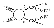
(a)      

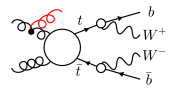
(b)      

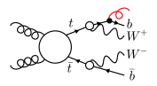
(c)      

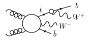
(d)      

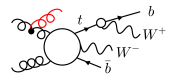
(e)      

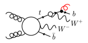
(f)      

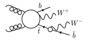
(g)      

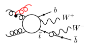
(h)      

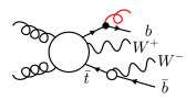
(i)      

Figure 1: Examples of resonance histories for the full process $gg\to W^{+}W^{-}b\bar{b}$. The three rows correspond to Born-level and real-emission histories associated with the production subprocesses $gg\to t\bar{t}$ (diagrams 1(a)–1(c)), $gg\to t\,W^{-}\bar{b}$ (diagrams 1(d)–1(f)), and $gg\to\bar{t}\,W^{+}b$ (diagrams 1(g)–1(i)). In each diagram, the blobs correspond to the decomposition of the full process into production and decay subprocesses according to a specific resonance history. Feynman diagrams have been generated with FeynGame. Harlander:2020cyh .

In the original POWHEG approach Nason:2004rx ; Frixione:2007vw there is no mechanism that guarantees (17), while the key idea behind the POWHEG–RES method Jezo:2015aia is to use alternative mappings that satisfy

$$\Delta q^{2}_{r}=0\,,$$ (18)

thereby avoiding any unphysical effect in the NLOPS modelling of resonant processes. The strategy of using mappings that preserve the resonance virtualities can be best understood in the narrow-width approximation (NWA), where the production and decay of unstable particles are factorised as separate subprocesses, which are connected trough intermediate unstable particles that remain exactly on-shell. For example, let us consider the process $gg\to t\bar{t}\to W^{+}W^{-}b\bar{b}$, which factorises into the production subprocess $gg\to t\bar{t}$ and the decay subprocesses $t\to W^{+}b$ and $\bar{t}\to W^{-}\bar{b}$, as illustrated in Fig. 11(a)–1(c). In the presence of QCD radiation, in order to keep the intermediate $t$ and $\bar{t}$ quarks exactly on-shell, in the $\Phi_{\mathrm{R},c}$ mappings that describe collinear radiation emitted by the production subprocess (Fig. 11(b)), the invariant masses of the $W^{+}b$ and $W^{-}\bar{b}$ systems can be preserved by handling the corresponding four-momenta as if they were on-shell final-state $t$ and $\bar{t}$ momenta. Vice versa, in the case of radiation stemming form a $t\to W^{+}b$ decay (Fig. 11(c)) the virtuality of the $t$ quark can be preserved by keeping fixed the full four-momentum of the $W^{+}bg$ system, as in the case of a pure top-decay process.

In general, in the NWA each process is characterised by a so-called resonance history, which corresponds to a well-defined combination of subprocesses consisting of a main production subprocess and a certain number of $1\to 2$ decay subprocesses. The latter can be independent of each other, or single steps of a decay chain. In the NWA, the resonance history provides the key for the consistent generation of QCD radiation. In practice, each subprocess radiates as an independent process, and the momenta of the unstable particles that connect the various subprocesses are always kept on-shell, i.e. $q_{\mathrm{R},r}^{2}=q_{\mathrm{B},r}^{2}=M_{r}^{2}$. This is achieved by handling the $q_{r}$ momenta on a similar footing as the external momenta of a hard scattering process.

Let us now move away from the NWA and consider exact NLO calculations of resonant processes, where finite-width effects are included throughout. In this case, intermediate unstable particles are no longer exactly on-shell. Moreover, each process with a well-defined initial and final state can involve multiple resonance histories that interfere with each other. For instance, the process $gg\to W^{+}W^{-}b\bar{b}$ involves, in addition to the above mentioned $gg\to t\bar{t}$ resonance history (Fig. 11(a)–1(c)), also resonance histories associated with the single-top production subprocesses $gg\to t\,W^{-}\bar{b}$ (diagrams 1(d)–1(f)), and $gg\to\bar{t}\,W^{+}b$ (diagrams 1(d)–1(f)). In this context, the strategy of the POWHEG–RES method is based on a probabilistic splitting of the full process into contributions that are each dominated by a well defined resonance history. In this way, within each resonance history, the condition (18) can be ensured by treating QCD radiation in a way that corresponds to an off-shell continuation of NWA approach. More explicitly, when unstable particles are off-shell, i.e. $q^{2}_{\mathrm{B},r}\neq M_{r}^{2}$, within each resonance history the emission of QCD radiation is organised in the same way as in corresponding NWA, but using NWA mappings that correspond to unstable particles with “modified masses” $M_{r}\to\sqrt{q^{2}_{\mathrm{B},r}}$. This automatically guarantees that $q^{2}_{\mathrm{R},r}=q^{2}_{\mathrm{B},r}$ in the vicinity of each resonance.

At Born level, the splitting into resonance histories is implemented as

$$B(\Phi_{\mathrm{B}})\,=\,\sum_{h\in\,\mathcal{H}}B_{h}(\Phi_{\mathrm{B}})\,,\qquad\mbox{with}\qquad B_{h}(\Phi_{\mathrm{B}})\,=\,\omega^{(\mathrm{hist})}_{h}(\Phi_{\mathrm{B}})\,B(\Phi_{\mathrm{B}})\,,$$ (19)

where the labels $r\in\mathcal{H}$ correspond to the different histories, i.e. $\mathcal{H}$ is the full set of resonance histories for the process at hand, while $\omega^{(\mathrm{hist})}_{h}(\Phi_{\mathrm{B}})\in[0,1]$ denote their phase-space dependent probabilities. The latter are determined as

$$\omega^{(\mathrm{hist})}_{h}(\Phi_{\mathrm{B}}) = \rho^{(\mathrm{hist})}_{h}(\Phi_{\mathrm{B}})\left[\sum_{h^{\prime}\in\mathcal{H}}\rho^{(\mathrm{hist})}_{h^{\prime}}(\Phi_{\mathrm{B}})\right]^{-1}\,,$$ (20)

where the weights $\rho^{(\mathrm{hist})}_{h}(\Phi_{\mathrm{B}})$ should mimic the relative probabilities of the different histories in the limit of small width. The first implementations of the POWHEG–RES method Jezo:2015aia ; Jezo:2016ujg are based on resonance weights of the form

$$\rho^{(\mathrm{hist})}_{h}(\Phi_{\mathrm{B}}) = \prod_{r\in\mathcal{R}(h)}\frac{M_{r}^{4}}{(q^{2}_{\mathrm{B},r}-M_{r}^{2})^{2}+\Gamma_{r}^{2}M_{r}^{2}}\,,$$ (21)

where the labels $r\in\mathcal{R}(h)$ correspond to the various resonances that contribute to the history $h$, while $M_{r}$, $\Gamma_{r}$, and $q_{\mathrm{B},r}\equiv q_{\mathrm{B},r}(\Phi_{\mathrm{B}})$ are, respectively, the rest mass, the width, and the four-momentum that flows through the propagator of the resonance $r$. A more realistic implementation of resonance histories based on Born matrix elements is presented in Sect. 4.2. In general, in the limit of vanishing decay widths, where all unstable particles go on-shell, any implementation of the resonance weights should obey

$$\lim_{\Gamma_{r}\,\to\,0}\;\rho^{(\mathrm{hist})}_{h}(\Phi_{\mathrm{B}}) \propto \prod_{r\in\mathcal{R}(h)}\delta(q_{\mathrm{B},r}^{2}-M_{r}^{2})\,,$$ (22)

which guarantees an exact correspondence of the probabilistic histories (20) with the uniquely-defined resonance histories of the NWA.

For the resonance-aware extension of the POWHEG formula (11), the weights (1) are split into different resonance-history contributions as

$$\bar{B}(\Phi_{\mathrm{B}})\,=\,\sum_{h\in\,\mathcal{H}}\bar{B}_{h}(\Phi_{\mathrm{B}})\qquad\mbox{with}\qquad\bar{B}_{h}(\Phi_{\mathrm{B}})\,=\,\omega^{(\mathrm{hist})}_{h}(\Phi_{\mathrm{B}})\,\bar{B}(\Phi_{\mathrm{B}})\,,$$ (23)

using the probabilities (20). As for the real-emission probabilities that are used to generate POWHEG emissions, the splitting (5) into collinear sectors is implemented at the level of individual resonance histories, i.e. the full real-emission weight is split into

$$R(\Phi_{\mathrm{R}}) = \sum_{h\in\mathcal{H}}\sum_{c\in\mathcal{C}(h)}R_{h,c}(\Phi_{\mathrm{R}})\,,$$ (24)

where the labels $c\in\mathcal{C}(r)$ correspond to the various collinear sectors that are consistent with the resonance history $h$. Such collinear sectors are in one-to-one correspondence with those for the on-shell production and decay process with history $h$ in the NWA. More explicitly, the sectors $c\in\mathcal{C}(h)$ correspond to all possible ways of emitting collinear radiation in the various production or decay “subprocess” of the history $h$. As discussed above, the associated $\Phi_{\mathrm{R},c}$ mappings are chosen in a way that preserves the virtuality of all resonances that belong to the history $h$. In this respect, we note that collinear sectors associated with the same collinear splitting but different resonance histories require, in general, different collinear mappings. Therefore, in order to avoid confusion, it is convenient to always label collinear sectors that are associated with different histories in a different way, i.e. all sectors should be labelled in such a way that $\mathcal{C}(h)\cap\mathcal{C}(h^{\prime})\,=\,\varnothing$  for $h^{\prime}\neq h$.

In analogy with (6) and (8), the contributions of the individual sectors in (24) are constructed as

$$R_{h,c}(\Phi_{\mathrm{R}})\,=\,\omega_{h,c}(\Phi_{\mathrm{R}})\,R(\Phi_{\mathrm{R}})\,,$$ (25)

with projectors

$$\omega_{h,c}(\Phi_{\mathrm{R}}) = \rho_{h,c}(\Phi_{\mathrm{R}})\left[\sum_{h^{\prime}\in\mathcal{H}}\sum_{c^{\prime}\in\mathcal{C}(h^{\prime})}\rho_{h^{\prime},c^{\prime}}(\Phi_{\mathrm{R}})\right]^{-1}\,,$$ (26)

and weights of the form

$$\rho_{h,c}(\Phi_{\mathrm{R}}) = \rho^{(\mathrm{hist})}_{h,c}(\Phi_{\mathrm{R}})\,\rho^{(\mathrm{coll})}_{c}(\widetilde{\Phi}_{\mathrm{rad},c})\,.$$ (27)

Here $\rho^{(\mathrm{coll})}_{c}$ are the usual collinear weights, with the only difference that, in the case of collinear splitting stemming from the decay of a resonance, the kinematic variables $\widetilde{\Phi}_{\mathrm{rad},\alpha}\equiv(\tilde{E}_{i},\tilde{E}_{j},\tilde{\theta}_{ij})$ are determined in the rest frame of the relevant resonance. As for the resonance weights $\rho^{(\mathrm{hist})}_{h,c}(\Phi_{\mathrm{R}})$, in Refs. Jezo:2015aia ; Jezo:2016ujg they have been chosen as

$$\rho^{(\mathrm{hist})}_{h,c}(\Phi_{\mathrm{R}}) = \prod_{r\in\mathcal{R}(h,c)}\frac{M_{r}^{4}}{(q^{2}_{\mathrm{R},r}-M_{r}^{2})^{2}+\Gamma_{r}^{2}M_{r}^{2}}\,,$$ (28)

which is the natural real-emission generalisation of (21). In this case, the labels $r\in\mathcal{R}(h,c)$ correspond to all resonances that are present in the resonance–collinear history $(h,c)$, while $q_{\mathrm{R},r}\equiv q_{\mathrm{R},r}(\Phi_{\mathrm{R}})$ is the four-momentum associated with a certain resonance. In practice, $q_{\mathrm{R},r}$ is the sum of all final-state momenta that flow through the propagator of the resonance $r$, including also real radiation that is emitted by the decay products of the resonance at hand in the collinear sector $c$. A matrix-element–based extension of such resonance weights will be presented in Sect. 4.2. In general, the real-emission resonance weights should always obey

$$\lim_{\Gamma\to 0}\;\rho^{(\mathrm{hist})}_{h,c}(\Phi_{\mathrm{R}}) \propto \prod_{r\in\mathcal{R}(h,c)}\delta(q^{2}_{\mathrm{R},r}-M_{r}^{2})\,,$$ (29)

which guarantees an exact correspondence of the probabilistic histories (26) with the uniquely-defined histories of the NWA. Beyond LO, this correspondence is crucial in order to ensure that, in the limit of small width, the full process factorises into separate production and decay subprocesses as in the NWA.

In the POWHEG–RES approach Jezo:2015aia , the POWHEG formula for the generation of LHEs assumes the form (23)

$$\mathrm{d}\sigma = \sum_{h\in\,\mathcal{H}}\,\bar{B}_{h}(\Phi_{\mathrm{B}})\,\mathrm{d}\Phi_{\mathrm{B}}\left[\Delta_{h}(q_{\operatorname{cut}})+\sum_{c\,\in\,\mathcal{C}(h)}\Delta_{h}(k_{\mathrm{T},c})\,\frac{R_{h,c}(\Phi_{\mathrm{R},c})}{B_{h}(\Phi_{\mathrm{B}})}\,\mathrm{d}\Phi_{\mathrm{rad},c}\right]\,,\qquad$$ (30)

where $B(\Phi_{\mathrm{B}})$, $\bar{B}(\Phi_{\mathrm{B}})$ and $R(\Phi_{\mathrm{R}})$ are split into resonance histories according to (19), (23) and (24), and LHEs are generated in the same way as in (11) but on a history-by-history basis. Similarly as in (12), the relevant Sudakov form factors are given by

$$\Delta_{h}(q_{\mathrm{T}}) = \exp\left[{}-\sum_{c\in\mathcal{C}(h)}\,\int\theta\left(k_{\mathrm{T},c}-q_{\mathrm{T}}\right)\,\frac{R_{h,c}(\Phi_{\mathrm{R},c})}{B_{h}(\Phi_{\mathrm{B}})}\,\mathrm{d}\Phi_{\mathrm{rad},c}\right]\,.$$ (31)

For the separation of resonance histories, the POWHEG formula (30) relies on the projectors (20) and (26), which are constructed in an approximate way. In this respect, we note that such projectors are only used to split the cross section into separate contributions, while the combination of all such contributions is consistent with the full $B(\Phi_{\mathrm{B}})$, $\bar{B}(\Phi_{\mathrm{B}})$ and $R(\Phi_{\mathrm{R}})$ weights, which are based on the exact matrix elements for the full set of resonant and non-resonant Feynman diagrams for the process at hand. In particular, the expansion of (30) to first order in $\alpha_{\rm S}$ beyond the leading order is identical to the result of a full NLO calculation.

The resonance-aware description of the hardest radiation can be further improved in a way that reflects the factorisation of higher-order radiative corrections into production and decay subprocesses in the narrow-width limit. This factorisation property allows one to generate one POWHEG emission from each production and decay subprocess that belongs to the resonance history of a given event Campbell:2014kua ; Jezo:2015aia ; Jezo:2016ujg . Therefore, in this approach, which is dubbed “all radiation” or allrad option in the POWHEG jargon, a LHE with history $h$ includes up to $n(h)$ POWHEG emissions, where $n(h)$ is one plus the number of decay subprocesses in the history $h$. For the bookkeeping of these multiple emissions, it is convenient to identify the associated production and decay subprocesses through history-dependent labels $s\in\mathcal{S}(h)$, where $\mathcal{S}(h)$ corresponds to the set of all subprocesses within the history $h$. In this way, the full set of collinear sectors $\mathcal{C}(h)$ can be split into subsectors $\mathcal{C}(s)\subset\mathcal{C}(h)$, where $c\in\mathcal{C}(s)$ corresponds to collinear radiation emitted within the subprocess $s\in\mathcal{S}(h)$, and $\mathcal{C}(h)\,=\,{\cup}_{s\in\mathcal{S}(h)}\,\mathcal{C}(s)\,$. With this notation, the allrad extension of the POWHEG–RES formula reads

$$\mathrm{d}\sigma = \sum_{h\in\,\mathcal{H}}\,\bar{B}_{h}(\Phi_{\mathrm{B}})\,\mathrm{d}\Phi_{\mathrm{B}}\prod_{s\,\in\,\mathcal{S}(h)}\left[\Delta_{s}(q_{\operatorname{cut}})+\sum_{c\,\in\,\mathcal{C}(s)}\Delta_{s}(k_{\mathrm{T},c})\,\frac{R_{h,c}(\Phi_{\mathrm{R},c})}{B_{h}(\Phi_{\mathrm{B}})}\,\mathrm{d}\Phi_{\mathrm{rad},c}\right]\,,\qquad$$ (32)

where each term between squared brackets corresponds to a separate POWHEG emission stemming from the subprocess $s\in\mathcal{S}(h)$ of the resonance history $h$. The Sudakov form factors $\Delta_{s}(q_{\mathrm{T}})$ are defined in the same way as in (31) but with $\mathcal{C}(h)$ replaced by $\mathcal{C}(s)$, i.e. including only radiation stemming from a specific production or decay subprocess. In the POWHEG–RES approach the $\Phi_{\mathrm{rad},c}$ radiation phase space is split into soft and hard parts. Similarly as in the original POWHEG method, this separation is controlled by the so-called ${\tt hdamp}$ parameter Alioli:2008tz , and the POWHEG–RES formulas (30) and (32) are used only to generate soft radiation. Instead, hard radiation is emitted without applying any Sudakov form factor and always as a single hard emission, i.e. disabling the allrad option. For simplicity, this different treatment of soft and hard radiation is not explicitly shown in the above formulas.

As for the matching of LHEs to parton showers, in the POWHEG–RES method Jezo:2015aia the standard matching approach is adapted to the resonance structure of the events. Specifically, for each LHE, all final-state partons are attributed to a corresponding production or decay subprocess $s\in\mathcal{S}(h)$, based on the resonance history $h$ of the event. The parton shower is then instructed to radiate in each production and decay subprocess in a way that preserves the virtuality of each resonance. Moreover, in the allrad approach the shower radiation that is emitted in the various subprocess $s$ is subject to different veto scales, which are given by the transverse momenta of the corresponding POWHEG emissions.

3 Spurious width effects in off-shell NLO and NLOPS cross sections

The POWHEG–RES method is designed according to the general factorisation properties of higher-order corrections in the NWA, which must be fulfilled also by off-shell calculations in the limit of small decay widths. In particular, when decay widths become small, the radiative corrections should factorise to all orders into contributions associated with the various production and decay subprocesses. Moreover, upon integration over the full phase space and summation over all possible decay channels, all decay probabilities must be equal to one. Thus, in the zero-width limit, the total cross section of the full off-shell process should be identical to the one of the associated production subprocess.

As pointed out in Refs. Melnikov:2009dn ; Hollik:2012rc ; Campbell:2012uf , this consistency property is not fulfilled by naive fixed-order implementations of the NWA. However, it can be ensured by means of a rigorous perturbative treatment of all terms that are inversely proportional to the decay widths of the resonant particles. In the following, this approach will be dubbed “inverse-width expansion”. Its application in the context of the NWA is discussed in Sect. 3.1, while in Sect. 3.2 we propose an extension of the inverse-width expansion to off-shell NLO calculations and their matching to parton showers in the POWHEG–RES framework.

3.1 Inverse-width expansion in the NWA

For simplicity, let us start with the case of a process that involves the production and decay of a single resonance. In the NWA, to all orders in perturbation theory, its differential cross section factorises as

$${\rm d}\sigma_{{\rm prod}\times{\rm dec}}\,=\,{\rm d}\sigma\frac{{\rm d}\Gamma}{\Gamma}\,,\quad\mbox{where}\quad\Gamma\,=\,\int\limits_{{\rm dec}}{}{\rm d}\Gamma\,.$$ (33)

Here $\sigma$ denotes the cross section for the production subprocess, while the integration is over the full decay phase space, and the sum over different decay channels is implicitly understood. As a result of this factorisation property, to all orders of perturbation theory the integral of the production$\times$decay cross section over the full decay phase space is equal to the production cross section, i.e.

$$\int\limits_{{\rm dec}}{\rm d}\sigma_{{\rm prod}\times{\rm dec}}\,=\,{\rm d}\sigma\,.$$ (34)

Let us now consider NLO calculations in the NWA, where the ingredients of (33) can be split into LO parts and NLO corrections as

$${\rm d}\sigma_{\mathrm{NLO}}\,=\,{\rm d}\sigma_{0}+{\rm d}\sigma_{1}\,,\qquad{\rm d}\Gamma_{\mathrm{NLO}}\,=\,{\rm d}\Gamma_{0}+{\rm d}\Gamma_{1}\,,\qquad\Gamma_{\mathrm{NLO}}\,=\,\Gamma_{0}+\Gamma_{1}\,.$$ (35)

If the $1/\Gamma$ term in (33) is not expanded, the NLO cross section is given by

$${\rm d}\sigma_{{{\rm prod}}\times{{\rm dec}}}^{\mathrm{NLO}}\,=\,{\rm d}\sigma_{0}\,\frac{{\rm d}\Gamma_{0}}{\Gamma_{\mathrm{NLO}}}+{\rm d}\sigma_{1}\,\frac{{\rm d}\Gamma_{0}}{\Gamma_{\mathrm{NLO}}}+{\rm d}\sigma_{0}\,\frac{{\rm d}\Gamma_{1}}{\Gamma_{\mathrm{NLO}}}\,,$$ (36)

and integrating over the decay phase space yields

$$\int\limits_{{\rm dec}}{}{\rm d}\sigma_{{{\rm prod}}\times{{\rm dec}}}^{\mathrm{NLO}}\,=\,\mathrm{d}\sigma_{0}\;\int\limits_{{\rm dec}}{}\frac{\mathrm{d}\Gamma_{\mathrm{NLO}}}{\Gamma_{\mathrm{NLO}}}\,+\,\mathrm{d}\sigma_{1}\;\int\limits_{{\rm dec}}{}\frac{\mathrm{d}(\Gamma_{\mathrm{NLO}}-\Gamma_{1})}{\Gamma_{\mathrm{NLO}}}\,=\,\mathrm{d}\sigma_{0}+\mathrm{d}\sigma_{1}-\mathrm{d}\sigma_{1}\frac{\Gamma_{1}}{\Gamma_{\mathrm{NLO}}}\,.$$ (37)

At variance with this naive approach, a consistent perturbative expansion of the inverse decay width Melnikov:2009dn ,

$$\frac{1}{\Gamma_{\mathrm{NLO}}}\,\to\,\frac{1}{\Gamma_{0}}\left(1-\frac{\Gamma_{1}}{\Gamma_{0}}\right)\,,$$ (38)

and its extension to the full production$\times$decay cross section, yields

$$\int\limits_{{\rm dec}}{}{\rm d}\sigma_{{{\rm prod}}\times{{\rm dec}}}^{\mathrm{NLO}_{\mathrm{exp}}} = \ \mathrm{d}\sigma_{0}\;\left[\left(1-\frac{\Gamma_{1}}{\Gamma_{0}}\right)\int\limits_{{\rm dec}}{}\frac{\mathrm{d}\Gamma_{0}}{\Gamma_{0}}\,+\int\limits_{{\rm dec}}{}\frac{\mathrm{d}\Gamma_{1}}{\Gamma_{0}}\right]\,+\,\mathrm{d}\sigma_{1}\;\int\limits_{{\rm dec}}{}\frac{\mathrm{d}\Gamma_{0}}{\Gamma_{0}}\;=\;\mathrm{d}\sigma_{0}+\mathrm{d}\sigma_{1}\,,\qquad$$ (39)

which is identical to the NLO production cross section, as expected from (34). In contrast, the “unexpanded” implementation (36) of the NWA deviates form the “expanded” one by the contribution

$${\rm d}\sigma_{\rm spurious}\,=\,-{\rm d}\sigma_{1}\frac{\Gamma_{1}}{\Gamma_{\mathrm{NLO}}}\,,$$ (40)

which violates the factorisation property (34) and is thus going to be denoted as “spurious”. Since this difference between the expanded and unexpanded versions of the NWA is of $\mathcal{O}(\alpha_{\rm S}^{2})$, in principle one may object that it does not violate (34) at NLO, and that it could be regarded as part of the NLO uncertainty. This perspective would make sense only if it was uncertain whether terms of the form (40) can contribute at NNLO or not. However, this is not the case, since in the perturbative expansion of  (34),

$$\int\limits_{{\rm dec}}{\rm d}\sigma={\rm d}\sigma_{0}+{\rm d}\sigma_{1}+{\rm d}\sigma_{2}+...\,,$$ (41)

it is clear that there is no room for terms that depend on the decay width. This can be easily understood also in the standard approach, where $1/\Gamma_{\mathrm{NLO}}$ is kept unexpanded. In this case, the spurious term (40) is exactly cancelled by a corresponding NNLO term,

$$\int\limits_{{\rm dec}}{}{\rm d}\sigma^{\mathrm{NLO}\times\mathrm{NLO}}_{{\rm prod}\times{\rm dec}}\,=\,{\rm d}\sigma_{1}\frac{\Gamma_{1}}{\Gamma_{\mathrm{NLO}}}\,,$$ (42)

which consists of the product of the $\mathcal{O}(\alpha_{s})$ corrections to $\mathrm{d}\sigma_{\rm prod}$ and $\mathrm{d}\Gamma$. For these reasons, the term (40) can be regarded as a spurious $\mathcal{O}(\alpha_{s}^{2})$ contribution, while the expanded result (39) guarantees a consistent implementation of the corrections to the decay subprocess, in the sense that the general properties (33)–(34) of the NWA are fulfilled order by order in perturbation theory.

We note that the consistency of the inclusive NWA cross section could also be guaranteed by keeping $1/\Gamma_{\mathrm{NLO}}$ unexpanded and including the product of the NLO corrections to production and decay, $\mathrm{d}\sigma_{1}\mathrm{d}\Gamma_{1}/\Gamma_{\mathrm{NLO}}$, into the NLO calculation. As compared to the inverse-width expansion (39), this alternative approach would yield the same inclusive cross section, but an improved differential description of NLO radiation in decays. However, its implementation is technically more involved.

Let us now consider the NWA for the production and decay of multiple resonances. In this case, to all orders in perturbation theory

$${\rm d}\sigma_{{\rm prod}\times{\rm dec}}={\rm d}\sigma\prod_{r\in\mathcal{R}}\frac{{\rm d}\Gamma_{r}}{\Gamma_{r}}\,,$$ (43)

where $\mathcal{R}$ is the set of intermediate unstable particles in the process at hand. The naive NLO implementation of the NWA corresponds to

$$\mathrm{d}\sigma_{{{\rm prod}}\times{{\rm dec}}}^{\mathrm{NLO}}\,=\,\left[\mathrm{d}\sigma_{0}+\sum_{r}\mathrm{d}\sigma_{0}\frac{\mathrm{d}\Gamma_{r,1}}{\mathrm{d}\Gamma_{r,0}}\,+\,\mathrm{d}\sigma_{1}\right]\left(\prod_{r\in\mathcal{R}}\frac{{\rm d}\Gamma_{r,0}}{\Gamma_{r,\mathrm{NLO}}}\right)\,.$$ (44)

Instead, extending the expansion to all $1/\Gamma_{r,\mathrm{NLO}}$ terms yields

$$\mathrm{d}\sigma_{{{\rm prod}}\times{{\rm dec}}}^{\mathrm{NLO}_{\mathrm{exp}}}\,=\,\left[\mathrm{d}\sigma_{0}+\sum_{r}\left(\mathrm{d}\sigma_{0}\frac{\mathrm{d}\Gamma_{r,1}}{\mathrm{d}\Gamma_{r,0}}-\mathrm{d}\sigma_{0}\frac{\Gamma_{r,1}}{\Gamma_{r,0}}\right)\,+\,\mathrm{d}\sigma_{1}\right]\left(\prod_{r\in\mathcal{R}}\frac{{\rm d}\Gamma_{r,0}}{\Gamma_{r,0}}\right)\,,$$ (45)

and it is easy to show that, similarly as in (39), integrating (45) over the decay phase space and summing over all decay channels, yields exactly the NLO cross section for the production process. In the context of top-quark pair production, this expansion approach was first proposed in Ref. Melnikov:2009dn and was also applied at NLO in Ref. Campbell:2012uf , and at NNLO in Ref. Czakon:2020qbd .

At NLO, the expanded version of the NWA can be related to the unexpanded one through

$$\mathrm{d}\sigma_{{{\rm prod}}\times{{\rm dec}}}^{\mathrm{NLO}_{\mathrm{exp}}} = \left(\prod_{r\in\mathcal{R}}\frac{\Gamma_{r,\mathrm{NLO}}}{\Gamma_{r,0}}\right)\mathrm{d}\sigma_{{{\rm prod}}\times{{\rm dec}}}^{\mathrm{NLO}}-\left(\sum_{r\in\mathcal{R}}\frac{\Gamma_{r,1}}{\Gamma_{r,0}}\right)\mathrm{d}\sigma_{{{\rm prod}}\times{{\rm dec}}}^{\mathrm{LO}}\,,$$ (46)

where

$$\mathrm{d}\sigma_{{{\rm prod}}\times{{\rm dec}}}^{\mathrm{LO}}\,=\,\mathrm{d}\sigma_{0}\left(\prod_{r\in\mathcal{R}}\frac{{\rm d}\Gamma_{r,0}}{\Gamma_{r,0}}\right)$$ (47)

is the LO cross section evaluated using the LO decay widths as input parameters. Using (46) one can express the spurious contribution for the case of multiple resonances as

$$\mathrm{d}\sigma_{\rm spurious} = \mathrm{d}\sigma_{{{\rm prod}}\times{{\rm dec}}}^{\mathrm{NLO}}-\mathrm{d}\sigma_{{{\rm prod}}\times{{\rm dec}}}^{\mathrm{NLO}_{\mathrm{exp}}}\,=\,\delta\kappa_{\rm spurious}\,\mathrm{d}\sigma_{{{\rm prod}}\times{{\rm dec}}}^{\mathrm{LO}}\,,$$ (48)

where

$$\delta\kappa_{\rm spurious} = \left[1-\left(\prod_{r\in\mathcal{R}}\frac{\Gamma_{r,\mathrm{NLO}}}{\Gamma_{r,0}}\right)\right]\kappa^{{\rm prod}\times{\rm dec}}_{\mathrm{NLO}}\;-\;\sum_{r\in\mathcal{R}}\frac{\Gamma_{r,1}}{\Gamma_{r,0}}\,,$$ (49)

with

$$\kappa^{{\rm prod}\times{\rm dec}}_{\mathrm{NLO}} = \frac{\mathrm{d}\sigma_{{{\rm prod}}\times{{\rm dec}}}^{\mathrm{NLO}}}{\mathrm{d}\sigma_{{{\rm prod}}\times{{\rm dec}}}^{\mathrm{LO}}}\,.$$ (50)

Here we see that the spurious correction factor (49) is a simple linear function of the differential NLO $K$-factor (50) with constant coefficients. Thus, $\delta\kappa_{\rm spurious}$ should feature a similarly mild kinematic dependence as the differential $K$-factor.

In order to estimate the typical size of $\delta\kappa_{\rm spurious}$, it is useful to simplify (49) by retaining only $\mathcal{O}(\alpha_{\rm S}^{2})$ terms of type $\mathrm{d}\sigma_{1}\Gamma_{r,1}$ and discarding terms beyond first order in $\Gamma_{r,1}$. This is justified by the fact that the QCD corrections to production processes are typically significantly bigger as compared to those for decays. In this approximation one can show that

$$\delta\kappa_{\rm spurious} \simeq {}-\frac{\mathrm{d}\sigma_{1}}{\mathrm{d}\sigma_{0}}\left(\sum_{r\in\mathcal{R}}\frac{\Gamma_{r,1}}{\Gamma_{r,0}}\right)\,,$$ (51)

where the sum between brackets corresponds to the relative effect of the corrections to all decay subprocesses. For processes that involve $t\bar{t}$ production, possibly in association with other particles, we have

$$\delta\kappa_{\rm spurious}^{t\bar{t}+X} \simeq {}-2\,\frac{\mathrm{d}\sigma_{1}}{\mathrm{d}\sigma_{0}}\frac{\Gamma_{t,1}}{\Gamma_{t,0}}\simeq{}+17\%\,\frac{\mathrm{d}\sigma_{1}}{\mathrm{d}\sigma_{0}}\,,$$ (52)

which can be a quite significant effect, depending on the size of the $K$-factor for the production subprocess. In general, if the corrections to the production subprocess are close to $100\%$, as in the case of $t\bar{t}b\bar{b}$ production Jezo:2018yaf , then $\delta\kappa_{\rm spurious}$ is as large as the total NLO correction to all decay subprocess. Thus, for any processes or kinematic region where $\mathrm{d}\sigma_{1}/\mathrm{d}\sigma_{0}$ is large, the NLO corrections to the involved decays are strongly distorted in the unexpanded NWA.

As we will see in Sect. 9, in the case of $t\bar{t}+tW$ production $\delta\kappa_{\rm spurious}$ is around $7\%$, which exceeds the size of the full $tW$ contribution. Thus, in order to avoid this misleading effect, in the next section we propose a generalisation of the expansion (45) to off-shell calculations.

3.2 Inverse-width expansion in off-shell calculations and POWHEG–RES matching

Let us now consider an off-shell process that involves (or is dominated by) a single resonance history, i.e. a single production subprocess and a single combination of chain decays. In the limit of small widths, the off-shell LO and NLO cross sections tend to the respective NWA cross sections, i.e.

$$\mathrm{d}\sigma_{\rm off-shell}^{\mathrm{(N)LO}}\,\underset{\Gamma_{r}\to 0}{\longrightarrow}\,\mathrm{d}\sigma_{{{\rm prod}}\times{{\rm dec}}}^{\mathrm{(N)LO}}\,.$$ (53)

Thus the inverse-width expansion (46) can be easily extended to the off-shell case by replacing the LO and NLO cross sections in the NWA by their off-shell counterparts. In addition, in order to ensure that the shapes of the various resonances are perfectly consistent with the corresponding NLO decay widths, $\mathrm{d}\sigma_{\rm off-shell}^{\mathrm{LO}}$ should be replaced by the Born contribution to the NLO cross section, which is computed using NLO instead of LO widths as input parameters. For this quantity we use the symbol $\mathrm{d}\sigma_{\rm off-shell}^{(0)}$, and the off-shell extension of the expansion (46) is given by

$$\mathrm{d}\sigma_{\rm off-shell}^{\mathrm{NLO}_{\mathrm{exp}}}\,=\,\left(\prod_{r\in\mathcal{R}}\frac{\Gamma_{r,\mathrm{NLO}}}{\Gamma_{r,0}}\right)\left[\mathrm{d}\sigma_{\rm off-shell}^{\mathrm{NLO}}-\left(\sum_{r\in\mathcal{R}}\frac{\Gamma_{r,1}}{\Gamma_{r,0}}\right)\mathrm{d}\sigma_{\rm off-shell}^{(0)}\right]\,,$$ (54)

where $\mathcal{R}(h)$ is the set of resonances that occur in the resonance history $h$. Note that here, at variance with (46), the product of $\Gamma_{r,\mathrm{NLO}}/\Gamma_{r,0}$ factors is applied both to $\mathrm{d}\sigma_{\rm off-shell}^{\mathrm{NLO}}$ and $\mathrm{d}\sigma_{\rm off-shell}^{(0)}$ since these two ingredients are both computed using NLO decay widths. By construction, the zero-width limit of (54) is equivalent to (46), and is thus consistent with the correct NLO production cross section.

Now we turn our discussion to an extension of the inverse-width expansion to the matching of off-shell NLO calculations in the POWHEG–RES framework. The aim of the prescription (54) is to restore the correct normalisation of the cross section, while POWHEG’s emission probabilities, i.e. the terms between square brackets in (30) and (32), have no net effect on the normalisation. Thus, in (30) and (32) the inverse-width expansion can be restricted to the $\bar{B}_{h}(\Phi_{\mathrm{B}})$ terms and implemented, in analogy with (54), as

$$\bar{B}_{h}(\Phi_{\mathrm{B}})\Big{|}_{\rm exp} = \left(\prod_{r\in\mathcal{R}(h)}\frac{\Gamma_{r,\mathrm{NLO}}}{\Gamma_{r,0}}\right)\left[\bar{B}_{h}(\Phi_{\mathrm{B}})-\left(\sum_{r\in\mathcal{R}(h)}\frac{\Gamma_{r,1}}{\Gamma_{r,0}}\right)B_{h}(\Phi_{\mathrm{B}})\right]\,.$$ (55)

Since $\bar{B}_{h}(\Phi_{\mathrm{B}})$ is the contribution of a specific resonance history $h\in\mathcal{H}$, its inverse-width expansion involves the widths of the corresponding resonances $r\in\mathcal{R}(h)$. Here we assume that the relevant building blocks, $B(\Phi_{\mathrm{B}})$, $V(\Phi_{\mathrm{B}})$ and $R(\Phi_{\mathrm{R}})$, have been constructed as usual, i.e. without inverse-width expansion, and using NLO widths as input parameters. Thus, all terms in (55), including the Born term $B_{h}(\Phi_{\mathrm{B}})$, are multiplied by the products of $\Gamma_{r,\mathrm{NLO}}/\Gamma_{r,0}$ factors between squared parentheses. This factor acts also to the virtual and real contributions to $\bar{B}(\Phi_{\mathrm{B}})$. Moreover it should be applied also to hard radiation as

$$R^{(\rm hard)}_{h,c}(\Phi_{\mathrm{R}})\Big{|}_{\rm exp} = \left(\prod_{r\in\mathcal{R}}\frac{\Gamma_{r,\mathrm{NLO}}}{\Gamma_{r,0}}\right)R^{(\rm hard)}_{h,c}(\Phi_{\mathrm{R}})\,,$$ (56)

where $R^{(\rm hard)}_{h,c}(\Phi_{\mathrm{R}})$ corresponds to the so-called hard remnant, i.e. real radiation “harder than ${\tt hdamp}$”, which is handled as fixed-order NLO radiation.

As demonstrated in Sect. 9, this inverse-width expansion has a quite significant impact on off-shell $t\bar{t}+tW$ production and decay cross sections. In particular, when comparing off-shell against on-shell $t\bar{t}+tW$ generators, the inverse-width expansion is absolutely crucial in order to avoid large spurious differences and to identify the remaining small differences that are due to physical off-shell effects.

4 Off-shell $t\bar{t}+tW$ production with dileptonic decays

In this section we briefly review the treatment of resonance histories in the original version of the bb4l generator Jezo:2016ujg , and we then introduce a new version of bb4l, which implements an extended set of resonance histories as well as improved resonance projectors based on matrix-element information, and the inverse-width expansion introduced in Sect. 3.

resonance history	production subprocess	decay subprocesses	examples
$t\bar{t}$	$pp\to t\bar{t}$	$t\to W^{+}b$	Fig. 11(a)–1(c)
		$\bar{t}\to W^{-}\bar{b}$
$tW^{-}$	$pp\to t\,W^{-}\bar{b}$	$t\to W^{+}b$	Fig. 11(d)–1(f)
$\bar{t}\,W^{+}$	$pp\to\bar{t}\,W^{+}b$	$\bar{t}\to W^{-}\bar{b}$	Fig. 11(g)–1(i)
$Z$	$pp\to Z/H+b\bar{b}$	$Z/H\to\ell^{+}\nu_{\ell}\,\ell^{\prime\,-}\bar{\nu}_{\ell^{\prime}}$

Table 1: List of the Born resonance histories for the off-shell dileptonic process (57) with corresponding labels and decomposition into production and decay subprocesses. The leptonic $W$-boson decays $W^{+}\to\ell^{+}\nu_{\ell}$ and $W^{-}\to\ell^{\prime\,-}\bar{\nu}_{\ell^{\prime}}$ are kept implicit.

The bb4l generator describes the family of dileptonic processes

$$pp\to\ell^{+}\nu_{\ell}\,\ell^{\prime\,-}\bar{\nu}_{\ell^{\prime}}b\bar{b}\,.$$ (57)

All process-dependent ingredients for the generation of events, i.e. the terms $B$, $V$ and $R$ in the various POWHEG formulas, are based on exact matrix-element input of $\mathcal{O}(\alpha_{s}^{2}\alpha^{4})$ at LO and $\mathcal{O}(\alpha_{s}^{3}\alpha^{4})$ at NLO. At Born level, the full process (57) involves four different resonance histories, which are listed in Tab. 1 and correspond to the production subprocesses $pp\to t\bar{t}$,  $pp\to tW^{-}\bar{b}$,  $pp\to\bar{t}\,W^{+}b$,  and $pp\to Z/H+b\bar{b}$, together with the respective decay subprocesses. For simplicity, we will collectively denote the $tW^{-}\bar{b}$ and $\bar{t}\,W^{+}b$ histories as $tW$ (or sometimes $tWb$) histories. In practice the $pp\to Z/H+b\bar{b}$ subprocess plays a negligible role, and the full process is completely dominated by the resonance histories of $t\bar{t}$ and $tW$ type. The latter are illustrated in Fig. 1, where leptonic $W$-boson decays are omitted for simplicity.

In the dileptonic bb4l generator the inverse-width expansion (55)–(56) is restricted to top resonances and is applied, depending on the resonance history, to one or two top quarks. Thus (55) yields correction factors $(\Gamma_{t,\mathrm{NLO}}/\Gamma_{t,0})^{n(h)}$ and $n(h)\,(\Gamma_{t,1}/\Gamma_{t,0})$ where $n(h)$ is the history-dependent number of top resonances. As for $W$ resonances, in the dileptonic process (57) they can not give rise to any spurious effects of type (49). This is due to the fact that leptonic $W$ decays do not receive any $\mathcal{O}(\alpha_{\rm S})$ correction. Thus, all matrix elements are evaluated using $\Gamma_{W,\mathrm{NLO}}$ throughout as input parameter, and without expanding $1/\Gamma_{W,\mathrm{NLO}}$. For a discussion of the inverse-width expansion in the case of semileptonic decays see Sect. 5.2.

4.1 The original bb4l generator

The implementation of the POWHEG–RES approach in the original version of the bb4l generator Jezo:2016ujg is based on a simplified treatment of the resonance structure of the process (57). In particular, instead of the full set of Born resonance histories listed in Tab. 1, only the $t\bar{t}$ and the $Z$ resonance histories have been considered. The role of the former was to guarantee a correct treatment of all top resonances, while the $Z$ history was meant to account for non-resonant contributions.

These two resonance histories have been implemented using naive projectors of type (21) and (28), including the relevant top, anti-top, $W$- and $Z$-boson resonances. In Ref. Jezo:2016ujg it was found that the $Z$ resonance history is suppressed at the sub-percent level. Thus almost all LHEs are generated according to the $t\bar{t}$ history in the original bb4l generator. This implies that, for almost all events, POWHEG and shower radiation is emitted in a way that preserves the virtuality of the $W^{+}b$ and $W^{-}\bar{b}$ pairs. Moreover, at the LHE level, the allrad approach (32) leads to three “factorised” QCD emissions: one from the $t\bar{t}$ production subprocess plus two extra emissions from the $t\to W^{+}b$ and $\bar{t}\to W^{-}\bar{b}$ decays. As discussed in more detail below, this treatment is well justified only for events of $t\bar{t}$ type, while in the original version of bb4l it is applied also to events of $tW$ type.

4.2 New bb4l-dl generator with improved resonance histories

In this section we present a new version of the bb4l generator that implements new resonance histories of $tW$ kind together with a more accurate determination of the resonance history projectors (20) and (26), based on matrix-element information. This new version of bb4l will be referred to as bb4l-dl, where “dl” stands for dileptonic, while its single-lepton extension introduced in Sect. 5 will be called bb4l-sl.

At variance with the original bb4l, in the new bb4l-dl generator the negligible $Z$ resonance history is discarded, while the dominant $t\bar{t}$ history is supplemented by the two subdominant resonance histories of $tW$ type, which were absent in the original version of bb4l. Thus bb4l-dl is based on the full set of resonance histories that dominate the process (57) in most regions of the phase space.

As discussed in Sect. 2.2, in each resonance history the kinematic mappings (2) need to be defined in such a way that collinear QCD radiation does not modify the virtuality of the relevant resonances. To this end, all mappings associated with the $t\bar{t}$ history have been kept as in the original bb4l generator, while in the case of the $tW^{-}\bar{b}$ ($\bar{t}W^{+}b$) histories novel mappings are used, where the non-resonant $W^{-}\bar{b}$ ($W^{+}b$) pairs are handled as part of the hard production subprocess, and only the virtuality of the resonant $t$ ($\bar{t}$) quarks is preserved.

The most significant difference between the original and the new version of bb4l lies in the treatment of QCD radiation stemming from events of $tW$ kind. On the one hand, the new $tW$ histories imply that events of $tW$ kind generate only two POWHEG emission in the allrad approach: one from the $pp\to tWb$ production subprocess and a second one from the decay of the top resonance. The generation of these two independent POWHEG emissions is justified by the factorisation properties of QCD radiation in the presence of a top resonance. On the other hand, in the original approach without $tW$ histories, events of $tW$ kind are treated in the same way as $t\bar{t}$ events. In the allrad approach, this leads to a third POWHEG emission that is generated by an off-shell $Wb$ pair in a way that is not supported by theoretical arguments. In fact, from the viewpoint of the correct $tW$ resonance structure, this third emission can violate the consistent ordering of QCD radiation in the $pp\to tWb$ production subprocess. Vice versa, with the new $tW$ resonance histories, the $pp\to tWb$ subprocess leads to a single POWHEG radiation followed by consistently ordered shower emissions.

For what concerns the implementation of the new resonance histories, in order to assign realistic $t\bar{t}$ and $tW$ probabilities and to assess the related ambiguities, we have considered two different types of history projectors: naive projectors of type (21) and improved projectors based on matrix elements.

Naive resonance projectors

As a first option we have considered resonance projectors of the same form (20)–(21) as in the original bb4l generator. At Born level, the weight of the $t\bar{t}$ history reads

$$\rho^{(\mathrm{hist})}_{t\bar{t}}(\Phi_{\mathrm{B}})\Big{|}_{\mathrm{naive}} = W_{t}(p_{t})W_{t}(p_{\bar{t}})\,,$$ (58)

with

$$W_{t}(p) = \frac{M_{t}^{4}}{(p^{2}-M_{t}^{2})^{2}+\Gamma_{t}^{2}M_{t}^{2}}\,,$$ (59)

where the top and anti-top momenta are given by $p_{t}=p_{b}+p_{\ell^{+}}+p_{\nu_{\ell}}$ and $p_{\bar{t}}=p_{\bar{b}}+p_{\ell^{{}^{\prime}-}}+p_{\bar{\nu}_{\ell^{\prime}}}$. In the case of $tW$ histories, one of the top propagators is absent. At the same time, in the dominant $gg$ channel, and in the dominant phase-space region for $tW$ production, the $gg\to W^{+}W^{-}b\bar{b}$ matrix elements involve an enhanced $t$-channel propagator that is associated with initial-state $g\to b\bar{b}$ splittings. In the collinear regions, the virtualities of such enhanced propagators correspond to the transverse energies of the $b$-quark spectators that are involved in the initial-state splittings, i.e.

$$E^{2}_{\mathrm{T},b} = m_{b}^{2}+p_{\mathrm{T},b}^{2}\,,\qquad\mbox{or}\qquad E^{2}_{\mathrm{T},\bar{b}}\,=\,m_{b}^{2}+p_{\mathrm{T},{\bar{b}}}^{2}\,.$$ (60)

Thus the weights for the $tW$ histories are defined as the product of the weights (59) for a single top or anti-top propagator combined with the $1/E^{2}_{\mathrm{T}}$ enhancements form the associated $g\to b\bar{b}$ splittings, i.e.

$$\rho^{(\mathrm{hist})}_{\bar{t}W^{+}}(\Phi_{\mathrm{B}})\Big{|}_{\mathrm{naive}} = \frac{\chi\,m_{t}^{2}}{E^{2}_{\mathrm{T},b}}\,{W_{t}(p_{\bar{t}})}\,,\qquad\rho^{(\mathrm{hist})}_{tW^{-}}(\Phi_{\mathrm{B}})\Big{|}_{\mathrm{naive}}\,=\,\frac{\chi\,m_{t}^{2}}{E^{2}_{\mathrm{T},\bar{b}}}\,{W_{t}(p_{t})}\,.$$ (61)

To be precise, in the resonance weights (58) and (61) we have also included extra contributions corresponding to the $W^{+}$ and $W^{-}$ propagators. However, such $W$ contributions are identical for all considered histories, and thus they cancel out in the resonance projectors (8) and (20). For what concerns (61), note that we have introduced a factor $\chi$, which can be adjusted in a way that the relative weights of the $t\bar{t}$ and $tW$ histories are in reasonably good agreement with the corresponding physical cross sections. This is not guaranteed for $\chi=1$, since the different nature of the Breit–Wigner and initial-state $g\to b\bar{b}$ enhancements implies the presence of different extra prefactors in (59) and (61).

The real-emission resonance weights $\rho^{(\mathrm{hist})}_{h,c}(\Phi_{\mathrm{R}})$ that enter (27) have been constructed as in (58)–(61), but replacing $p_{b}\to p_{b}+p_{g}$ or $p_{\bar{b}}\to p_{\bar{b}}+p_{g}$ in the collinear sectors that involve the corresponding splittings.

Matrix-element based resonance projectors

For a more accurate separation of the resonance histories of $t\bar{t}$ and $tW$ type we have implemented improved resonance projectors based on matrix elements. To this end, we have split the $q\bar{q}$ and gluon–gluon Born amplitudes of the full process (57) according to their resonance structure as

$$\mathcal{A}_{\mathrm{full}}\,=\,\mathcal{A}_{t\bar{t}}\,+\,\mathcal{A}_{\bar{t}W^{+}}\,+\,\mathcal{A}_{tW^{-}}\,+\,\mathcal{A}_{\mathrm{rem}}\,.$$ (62)

Here the summands on the rhs correspond to the subsets of Feynman diagrams that contain: two (anti)top resonances ($\mathcal{A}_{t\bar{t}}$), a single top ($\mathcal{A}_{\bar{t}W^{+}}$) or anti-top ($\mathcal{A}_{tW^{-}}$) resonance, and no top resonance at all ($\mathcal{A}_{\mathrm{rem}}$). In general, this splitting is not gauge invariant. However, it ensures a gauge-invariant separation of double and single-top processes in the phase-space regions that are strongly dominated by on-shell $t\bar{t}$ or $tW$ production. For the separation of the various resonance histories, we have employed the corresponding squared matrix elements, i.e.

$$\rho^{(\mathrm{hist})}_{t\bar{t}}(\Phi_{\mathrm{B}})\big{|}_{\mathrm{ME}} = |\mathcal{A}_{t\bar{t}}|^{2}\,,\qquad$$

$$\rho^{(\mathrm{hist})}_{\bar{t}W^{+}}(\Phi_{\mathrm{B}})\big{|}_{\mathrm{ME}} = |\mathcal{A}_{\bar{t}W^{+}}|^{2}\,,$$

$$\rho^{(\mathrm{hist})}_{tW^{-}}(\Phi_{\mathrm{B}})\big{|}_{\mathrm{ME}} = |\mathcal{A}_{tW^{-}}|^{2}\,.$$ (63)

In this definition of resonance projectors, all non-resonant (i.e. free from any top resonance) effects, as well as interferences between $t\bar{t}$, $tW$ and non-resonant contributions are neglected under the assumption that they play only a subleading role. In the following, all non-resonant and interference contributions will be simply referred to as interference effects, since they are dominated by the interference between $t\bar{t}$ and $tW$ channels.

In the phase-space regions that are dominated either by $t\bar{t}$ or $tW$ production, interference effects are expected to be suppressed. However, in the off-shell phase space that separates the $t\bar{t}$ from the $tW$ dominated regions, interference effects can play a significant role. In this case, the resonance weights (4.2) may involve a significant ambiguity due to the fact that interference effects are assigned to the $t\bar{t}$ or $tW$ histories in an uncontrolled way. In order to quantify this ambiguity we have considered two alternative resonance-history definitions, where the interference effects are explicitly assigned to one of the histories. The first alternative is given by the weights

$$\rho^{(\mathrm{hist})}_{t\bar{t}}(\Phi_{\mathrm{B}})\big{|}_{\mathrm{ME}^{\prime}} = |\mathcal{A}_{\mathrm{full}}|^{2}-|\mathcal{A}_{\bar{t}W^{+}}|^{2}-|\mathcal{A}_{\bar{t}W^{+}}|^{2}\,,$$

$$\rho^{(\mathrm{hist})}_{\bar{t}W^{+}}(\Phi_{\mathrm{B}})\big{|}_{\mathrm{ME}^{\prime}} = |\mathcal{A}_{\bar{t}W^{+}}|^{2}\,,$$

$$\rho^{(\mathrm{hist})}_{tW^{-}}(\Phi_{\mathrm{B}})\big{|}_{\mathrm{ME}^{\prime}} = |\mathcal{A}_{tW^{-}}|^{2}\,,$$ (64)

which effectively assign all interference effects to the $t\bar{t}$ history, while the second alternative is given by

$$\rho^{(\mathrm{hist})}_{t\bar{t}}(\Phi_{\mathrm{B}})\big{|}_{\mathrm{ME}^{\prime\prime}} = |\mathcal{A}_{t\bar{t}}|^{2}\,,\qquad$$

$$\rho^{(\mathrm{hist})}_{\bar{t}W^{+}}(\Phi_{\mathrm{B}})\big{|}_{\mathrm{ME}^{\prime\prime}} = |\mathcal{A}_{\bar{t}W^{+}}|^{2}\,,$$

$$\rho^{(\mathrm{hist})}_{tW^{-}}(\Phi_{\mathrm{B}})\big{|}_{\mathrm{ME}^{\prime\prime}} = |\mathcal{A}_{tW^{-}}|^{2}\,,$$

$$\rho^{(\mathrm{hist})}_{\mathrm{rem}}(\Phi_{\mathrm{B}})\big{|}_{\mathrm{ME}^{\prime\prime}} = |\mathcal{A}_{\mathrm{full}}|^{2}-|\mathcal{A}_{t\bar{t}}|^{2}-|\mathcal{A}_{\bar{t}W^{+}}|^{2}-|\mathcal{A}_{tW^{-}}|^{2}\,,$$ (65)

where interference effects are excluded from the $t\bar{t}$ and $tW$ histories, and are assigned to an additional “remainder” history (rem).

	naive		matrix-element–based			extrapolation
	$\chi=1$	$\chi=0.1$	$\mathrm{ME}$	$\mathrm{ME}^{\prime}$	$\mathrm{ME}^{\prime\prime}$	$\Gamma_{t}\to 0$
$t\bar{t}$	90.6%	95.3%	94.2%	93.7%	95.3%	96.0%
$tW$	9.4%	4.7%	5.8%	6.3%	6.2%	$4.0\%$
rem					${}-1.5$%

Table 2: Relative contributions of different resonance histories to the total LO cross section for the full processes $pp\to\ell^{+}\nu_{\ell}\,\ell^{\prime\,-}\bar{\nu}_{\ell^{\prime}}b\bar{b}$ at 13 TeV. The first two columns correspond to the “naive” $t\bar{t}$ and $tW$ resonance histories defined in (58)–(61) for two different values of the normalisation parameter $\chi$. The last three columns correspond to the matrix-element resonance histories defined in (4.2)–(4.2). The $\mathrm{ME}^{\prime\prime}$ variant defined in (4.2) involves also a remainder history (“rem”), which embodies all interference and non-resonant contributions.

For the separation of real emission into resonance histories, the Born weights (4.2) and their variants (4.2)–(4.2) have been extended to the real-emission phase space according to

$$\rho^{(\mathrm{hist})}_{h,c}(\Phi_{\mathrm{R}})\big{|}_{\mathrm{ME}} = \rho^{(\mathrm{hist})}_{h}(\widetilde{\Phi}_{\mathrm{B},c})\big{|}_{\mathrm{ME}}\,,$$ (66)

where the lhs corresponds to the weight that enters (27), and the Born events $\widetilde{\Phi}_{\mathrm{B},c}$ on the rhs are defined through special real-to-Born mappings,

$$\widetilde{\Phi}_{\mathrm{B},c}\,\equiv\,\widetilde{\Phi}_{\mathrm{B},c}(\Phi_{\mathrm{R}})\,,$$ (67)

which are defined in a way that preserves the relative probabilities of $t\bar{t}$ and $tW$ histories. This can not be achieved by inverting the standard collinear mappings, since such mappings can lead to severe distortions of the virtualities of the enhanced $t$-channel propagators associated with initial-state $g\to b\bar{b}$ splittings within $tW^{-}\bar{b}$ ($\bar{t}W^{+}b$) resonance histories. For this reason we have designed dedicated real-to-Born mappings (67) that simultaneously preserve the virtualities of the resonant top quarks and $W$ bosons, and also, as far as possible, the transverse energies of the $b$- or $\bar{b}$-quark emitters, according to the collinear sector at hand. Such mappings can be found in App. A and are only used for the construction of the resonance weights (66).

In order to quantify the ambiguity that is related to the treatment of interference effects, we have compared the contributions of the various resonance histories defined in (58)–(61) and (4.2)–(4.2) to the LO cross section for the full process (57). As shown in Tab. 2, the naive resonance histories (58)–(61) yield $t\bar{t}$ and $tW$ fractions that are strongly sensitive to the choice of the free normalisation parameter $\chi$. At the level of the total cross section, setting $\chi\simeq 0.1$ yields a reasonable $tW$ fraction. However, this choice is not guaranteed to provide a consistent $t\bar{t}$ – $tW$ separation in the presence of arbitrary cuts and for any differential observable. For this reason, matrix-element based resonance histories are certainly preferable. In this case, the three different options defined in (4.2)–(4.2) yield fairly consistent $tW$ fractions, which vary between $5.8\%$ and $6.3\%$. Comparing the $\mathrm{ME}^{\prime}$ and $\mathrm{ME}^{\prime\prime}$ histories, as expected we observe almost identical $tW$ fractions, while the different treatments of $t\bar{t}$ histories and interference effects give rise to significant deviations in the corresponding fractions. In the $\mathrm{ME}^{\prime\prime}$ case, the “rem” channel embodies all interference effects, which turn out to be negative and amount to $-1.5\%$, while the “pure” $t\bar{t}$ channel corresponds to $95.3\%$. Vice versa, in the $\mathrm{ME}^{\prime}$ case all interference effects are attributed to the $t\bar{t}$ channel, which is thus shifted by about $-1.5\%$ as compared to the $\mathrm{ME}^{\prime\prime}$ case. As for the $\mathrm{ME}$ case, comparing against $\mathrm{ME}^{\prime\prime}$ we observe that the interference effects are shared between the $t\bar{t}$ and $tW$ channels with contributions that amount, respectively, to $-1.1\%$ and $-0.4\%$ of the total LO cross section.

In order to demonstrate that the new matrix-element–based projectors provide a reasonably well defined separation between $t\bar{t}$ and $tW$ contributions, we have compared the various matrix-element–based fractions reported in Tab. 2 against an alternative separation based on the $\Gamma_{t}\to 0$ extrapolation (see e.g. Cascioli:2013wga ) of the LO cross section for the full process (57). The key idea is that, in the limit where the total top-decay width is sent to zero, the $t\bar{t}$ contribution ($|\mathcal{A}_{t\bar{t}}|^{2}$) to the integrated cross section scales like $1/\Gamma_{t}^{2}$, while $tW$ contributions and $t\bar{t}$–$tW$ interferences scale like $1/\Gamma_{t}$. Thus, the $t\bar{t}$ contribution can be defined in a gauge-invariant way as

$$\sigma_{t\bar{t}}\,=\,\lim_{\xi_{t}\to 0}\left(\xi_{t}^{2}\,\sigma_{\mathrm{bb4l}}\Big{|}_{\Gamma_{t}\to\xi_{t}\Gamma_{t}}\right)\,.$$ (68)

For the LO cross section at 13 TeV, performing a numerical $\Gamma_{t}\to 0$ extrapolation we found

$$\frac{\sigma_{t\bar{t}}}{\sigma_{\mathrm{bb4l}}}\,=\,96.0\%\,,\qquad\frac{\sigma_{\mathrm{non-}t\bar{t}}}{\sigma_{\mathrm{bb4l}}}\,=\,1-\frac{\sigma_{t\bar{t}}}{\sigma_{\mathrm{bb4l}}}\,=\,4.0\%\,.$$ (69)

This separation is expected to be equivalent to the one provided by the $\mathrm{ME}^{\prime\prime}$ resonance histories, since in both cases the $t\bar{t}$ channel and its complement correspond to the contributions stemming from $|\mathcal{A}_{t\bar{t}}|^{2}$ and $|\mathcal{A}_{\mathrm{full}}-\mathcal{A}_{t\bar{t}}|^{2}$, respectively. However, contrary to the $\mathrm{ME}^{\prime\prime}$ approach, the definition of the $t\bar{t}$ contribution (68) involves also the narrow-width limit. Still, the $t\bar{t}$ fractions obtained with the $\mathrm{ME}^{\prime\prime}$ resonance histories and the $\Gamma_{t}\to 0$ extrapolation turn out to agree at the few permil level. Of course, the same level of agreement is also found between the non-$t\bar{t}$ parts in (69) and the combination of the $tW$ and remainder histories of $\mathrm{ME}^{\prime\prime}$ type.

These findings, together with the comparison in Tab. 2, demonstrate that matrix-element–based resonance histories provide a sound separation of the full process (57) into contributions of $t\bar{t}$ and $tW$ kind. This separation is not exact due to the unavoidable ambiguities that are related to the assignment of interference effects. However, such ambiguities can be controlled in a systematic way through the definition of resonance histories, and in the case of the integrated cross section they turn out to be quite small.

We note in passing that the $t\bar{t}$ and $tW$ resonance histories of the new bb4l generator may also be exploited for applications that go beyond the generation of POWHEG radiation. For example, the fact that LHEs are assigned, by construction, to a specific resonance history makes it possible to split bb4l event samples into $t\bar{t}$ and $tW$ subsamples in a way that bears similarities with the separation of different processes based on the matrix-element method Kondo:1988yd .

Finally, we note that the introduction of resonance histories with independent $t\bar{t}$ and $tW$ channels has required some technical improvements in the POWHEG BOX RES integrator. In the original setup the integrator adaptive sampling grids have been optimised using an average of grids over all resonance histories weighted by the cross sections in the individual resonance histories. This strategy works well if the average grid is well suited for all resonance histories that yield a significant contribution to the total cross section. This is not the case with the new resonance histories, and with the original integration approach the $tW$ histories feature a poor convergence already at LO. For this reason, we modified the POWHEG BOX RES integrator such that each resonance history provides an independent integration grid. In this way, the relative error in the cross section is each resonance history is roughly the same, and the total relative error is a much steeper function of the number of calls as compared to the case with only one grid.

5 Off-shell $t\bar{t}+tW$ production with semileptonic decays

In this section we present the new bb4l-sl version of the bb4l generator, which describes off-shell $t\bar{t}$ and $tW$ production with semileptonic decays. This reaction is part of the full process

$$pp\to\ell^{\pm}\nu_{\ell}jjb\bar{b}\,,$$ (70)

which involves a variety of other QCD and electroweak reactions. As will be discussed in Sect. 5.1, the contributions associated with $t\bar{t}$ and $tW$ production can be separated from the remaining contributions in a way that is free from any significant ambiguity due to interferences. Based on this observation, which is the outcome of a detailed analysis presented in App. B, we will select the physics content of the new bb4l-sl generator, i.e. the contributing perturbative orders, partonic processes and Feynman diagrams, in a way that corresponds to a direct generalisation of the original bb4l-dl generator. The implementation of the bb4l-sl generator is described in Sects. 5.2–5.3.

5.1 Selection of $t\bar{t}$ and $tW$ contributions to $\ell^{\pm}\nu_{\ell}jjb\bar{b}$ production

$\alpha_{\rm S}^{n}\alpha^{m}$	dominant subprocesses	type	order
$\alpha_{\rm S}^{4}\alpha^{2}$	$W^{\pm}b\bar{b}$ + 2 jets	$V$+HF	NNLO
$\alpha_{\rm S}^{3}\alpha^{3}$	tiny interference
$\alpha_{\rm S}^{2}\alpha^{4}$	$t\bar{t}+tWb$	$t\bar{t}+tW$	4FNS LO
	$gq\to tq^{\prime}\bar{b}$ + 1 jet	$t$-chanel single-top	4FNS NLO
	$q\bar{q}^{\prime}\to t\bar{b}$ + 2 jets	$s$-chanel single-top	NNLO
	$W^{\pm}Z$ + 2 jets with $Z\to b\bar{b}$	$VV$	NNLO
	$W^{\pm}jj$ + 2 $b$-jets	VBF	NNLO
$\alpha_{\rm S}^{1}\alpha^{5}$	tiny interference
$\alpha^{6}$	$W^{\pm}Zjj$ with $Z\to b\bar{b}$	VBS	LO
	$W^{\pm}ZV$ with $Z\to b\bar{b}$, $V\to jj$	$VVV$	LO

Table 3: Dominant processes in the Born cross section for $pp\to\ell^{\pm}\nu_{\ell}jjb\bar{b}$ at the various orders $\alpha_{\rm S}^{4-n}\alpha^{2+n}$ for $0\leq n\leq 4$. The last two columns indicate, respectively, the corresponding hard process (without light-jet emissions) and the order in QCD perturbation theory at which it starts contributing to the $pp\to\ell^{\pm}\nu_{\ell}jjb\bar{b}$ Born cross section. For instance, the vector-boson plus heavy flavour ($V$+HF) process $pp\to W^{\pm}b\bar{b}$ starts contributing at NNLO. See the main text for more details.

The Born cross section for the process (70) involves a tower of five different perturbative contributions, which range from $\mathcal{O}(\alpha_{\rm S}^{4}\alpha^{2})$ to $\mathcal{O}(\alpha^{6})$, and originate from the interplay of scattering amplitudes of order $g_{\rm S}^{4}e^{2}$, $g_{\rm S}^{2}e^{4}$ and $e^{6}$. As summarised in Tab. 3, the physics content of the individual squared Born terms is as follows.

• The terms of $\mathcal{O}(\alpha_{\rm S}^{4}\alpha^{2})$ represent the leading QCD contributions and originate form squared matrix elements of order $g_{\rm S}^{4}e^{2}$. They are dominated by $W$-boson plus heavy-flavour production ($W$+HF) in association with two additional light jets, i.e. $pp\to W^{\pm}b\bar{b}jj$, where the $W$ boson decays leptonically.

• The terms of $\mathcal{O}(\alpha_{\rm S}^{2}\alpha^{4})$ arise from squared matrix elements of order $g_{\rm S}^{2}e^{4}$ as well as from the interference between matrix elements of order $g_{\rm S}^{4}e^{2}$ and $e^{6}$. Such interferences are strongly colour-suppressed and are seven orders of magnitude smaller wrt the full $\mathcal{O}(\alpha_{\rm S}^{2}\alpha^{4})$ cross section. The latter is dominated by $t\bar{t}$ and $tW$ production, i.e. $pp\to W^{+}W^{-}b\bar{b}$, with one leptonic and one hadronic $W$-boson decay. Further subleading contributions are listed in Tab. 3 and are discussed in more detail below and in App. B.

• The terms of $\mathcal{O}(\alpha^{6})$ arise from squared matrix elements of order $e^{6}$ and represent the lowest order in $\alpha_{\rm S}$. They are dominated by the vector-boson scattering (VBS) process $pp\to W^{\pm}Zjj$ and the tri-boson production processes $pp\to W^{\pm}ZV$, with $Z\to b\bar{b}$ and a leptonically decaying $W$ boson, while in the tri-boson process the vector boson $V=Z,W^{\pm}$ decays into two jets.

The additional contributions of $\mathcal{O}(\alpha_{\rm S}^{5}\alpha^{3})$ and $\mathcal{O}(\alpha_{\rm S}^{3}\alpha^{5})$ correspond to pure interferences between matrix elements of different order. Such interferences are strongly suppressed due (also) to colour-interference effects. Thus, the contributions (i)–(iii) can be regarded as three separate processes, and only (ii) is included in bb4l-sl, while (i) and (iii) can be described through independent generators. The exact physics content of the bb4l-sl generator is defined as the subset of the ingredients of the full process (70), which results from the following three-step selection:

1. Only terms of $\mathcal{O}(\alpha_{\rm S}^{2}\alpha^{4})$ at LO and $\mathcal{O}(\alpha_{\rm S}^{3}\alpha^{4})$ at NLO are included;

2. The two light jets in the final state are required to contain a $q\bar{q}^{\prime}$ pair with quark flavours consistent with a $W^{\mp}\to q\bar{q}^{\prime}$ decay;

3. Only LO and NLO topologies that are in one-to-one correspondence with those occurring in the related dileptonic process (57) are included, with the addition, as detailed below, of NLO QCD corrections associated with the $q\bar{q}^{\prime}$ pair.

As discussed below, and in more detail in App. B, this selection is free from possible ambiguities due to interferences. Moreover it provides a good approximation of the full process (70) in phase-space regions where the invariant mass of the dijet system is not too far from $m_{W}$, i.e. in the regions that are usually selected for experimental measurements of $t\bar{t}$ and/or $tW$ production.

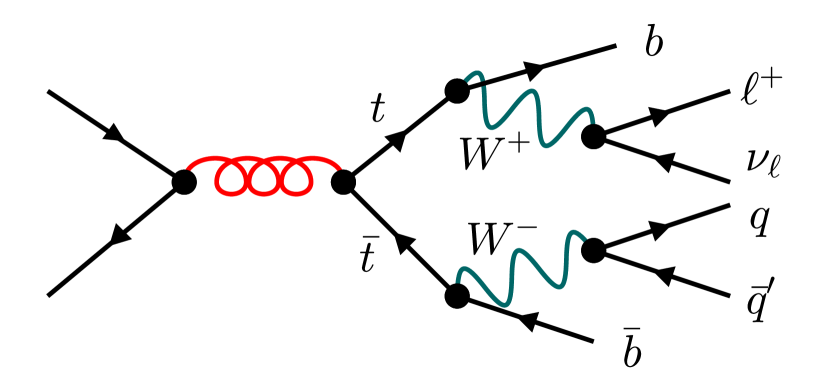
(a) $pp\to t\bar{t}$

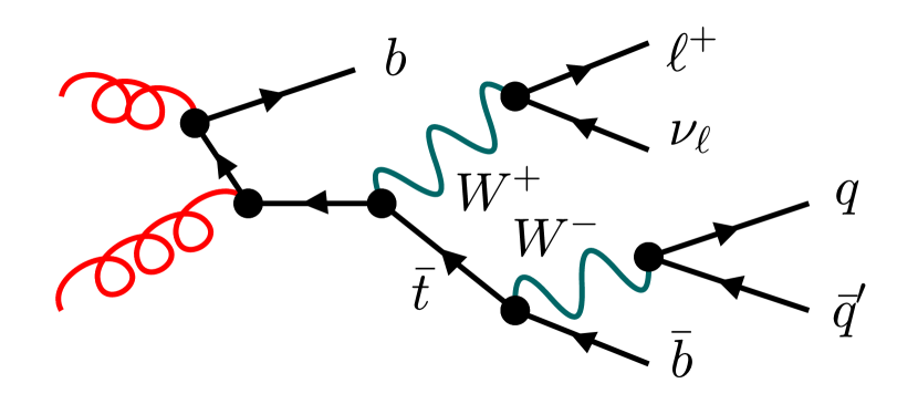
(b) $pp\to\bar{t}W^{+}b$

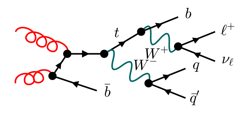
(c) $pp\to tW^{-}\bar{b}$

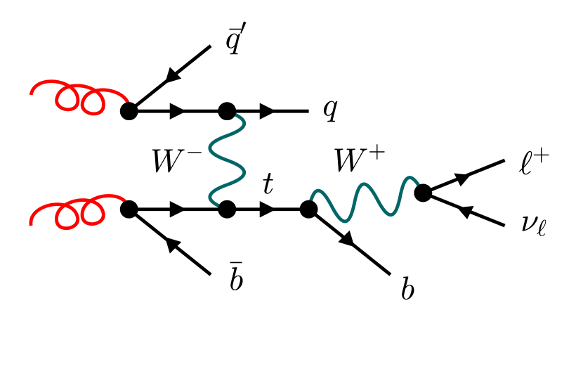
(d) $pp\to tj+2$ jets

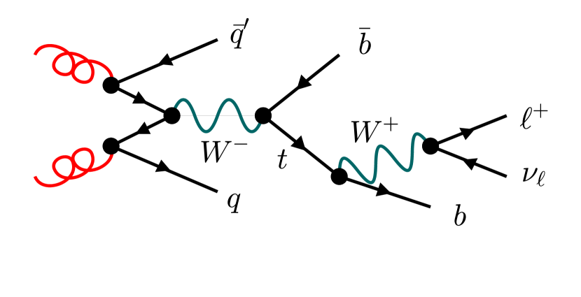
(e) $pp\to t{\bar{b}}+2$ jets

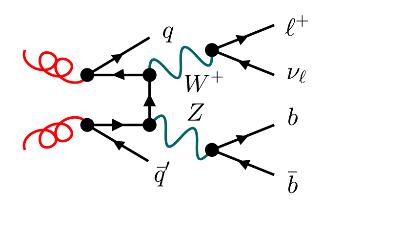
(f) $pp\to W^{+}Z(b\bar{b})+2$ jets

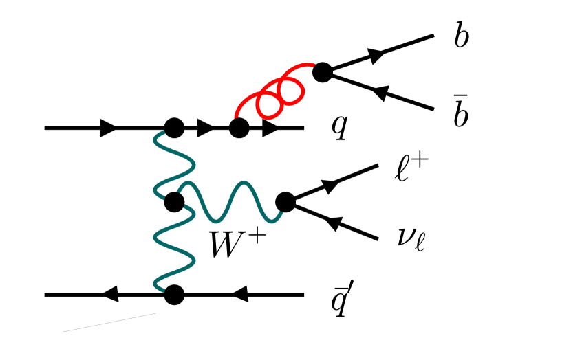
(g) $pp\;\xrightarrow[\mathrm{VBF}]{}\;W^{+}jj+2$ $b$-jets

Figure 2: Representative tree diagrams for various $\mathcal{O}(\alpha_{\rm S}^{2}\alpha^{4})$ contributions to $pp\to\ell^{\pm}\nu_{\ell}q\bar{q}^{\prime}b\bar{b}$. See the main text for more details.

Let us first consider the contributions that fulfill the criteria S1 and S2, i.e. the $\mathcal{O}(\alpha_{\rm S}^{2}\alpha^{4})$ and $\mathcal{O}(\alpha_{\rm S}^{3}\alpha^{4})$ contributions to

$$pp\to\ell^{\pm}\nu_{\ell}q\bar{q}^{\prime}b\bar{b}\,,$$ (71)

where in the case of a negatively (positively) charged lepton the $q\bar{q}^{\prime}$ pair must be consistent with the decay of a $W^{+}\,(W^{-})$ boson, i.e. $q\bar{q}^{\prime}\,=\,u\bar{d}\,(d\bar{u})$ or $c\bar{s}\,(s\bar{c})$. Note that the selection of this quark-flavour configuration is infrared safe at NLO. At this order, the process (71) involves all possible contributions and interference effects that can arise from $t\bar{t}$ or $tW$ production with semileptonic decays. Examples of the corresponding Born diagrams are depicted in Figs. 22(a)–2(c), while the remaining diagrams in Fig. 2, see also Tab. 3, correspond to various other physics processes that contribute to (71) at $\mathcal{O}(\alpha_{\rm S}^{2}\alpha^{4})$. These include $t$-channel single-top production in the 4FNS at NLO, i.e. with one extra jet (Fig. 22(d)), $s$-channel single-top production at NNLO, i.e. with two extra jets (Fig. 22(e)), $pp\to WZ(b\bar{b})$ at NNLO (Fig. 22(f)), and $Wjj$ production via vector-boson fusion with an extra $b\bar{b}$ pair (Fig. 22(g)). Formally all these different processes contribute to the same $\mathcal{O}(\alpha_{\rm S}^{2}\alpha^{4})$ and $\mathcal{O}(\alpha_{\rm S}^{3}\alpha^{4})$ cross section interfering with each other. Thus, in principle, they would have to be collectively treated as a single off-shell process. However, as shown in detail in App. B, the process (71) can be well approximated as the incoherent sum of two ingredients: on the one side a process corresponding to off-shell $t\bar{t}+tW$ production with interference and, on the other side, all other processes. In phase-space regions dominated by $t\bar{t}+tW$ production this approximation in fact holds at the permil level.

Based on this observation, in step S3 of our process definition we select all $t\bar{t}+tW$ contributions and interferences while discarding all other processes. Technically, at NLO this is achieved through the following two steps: (a) selecting the subset of semileptonic Feynman diagrams that originate from the full set of diagrams for the dileptonic process (57) by replacing a lepton-neutrino pair with a $q\bar{q}^{\prime}$ pair with the same weak-isospin quantum numbers; (b) adding, as described below, extra virtual and real-emission contributions associated with the QCD interactions of the $q\bar{q}^{\prime}$ pair. Schematically, this process definition can be written as

$$pp\,\to\,\ell^{\pm}\nu_{\ell}\ell^{\prime\mp}\nu_{\ell^{\prime}}b\bar{b}\,\bigg{|}_{\ell^{\prime\mp}\nu_{\ell^{\prime}}\;\rightarrow\;q\bar{q}^{\prime}}\;.$$ (72)

Since it is based on the full set of Feynman diagrams for the dileptonic process, this selection is guaranteed to be gauge invariant. At the NLO, the same conversion (72) is applied also to the virtual and real corrections.

Regarding the additional NLO corrections that arise when the lepton-neutrino pair is converted into a $q\bar{q}^{\prime}$ pair, we note that the $q\bar{q}^{\prime}$ fermionic line, which was originally a leptonic line, couples only to electroweak bosons and does not exchange any SU(3) colour with the other QCD partons. For this reason, the NLO corrections that are inherited from the dileptonic process via (72) do not interfere with the additional QCD corrections that result from the interaction of virtual and real gluons with the $q\bar{q}^{\prime}$ fermionic line. Based on this observation, we handle these extra QCD corrections as a separate contribution, which is directly implemented in the POWHEG–RES framework, as explained in the next section. For efficiency reasons, for the relevant matrix elements we use a $W^{+}W^{-}b\bar{b}$ double-pole approximation (DPA), where we include only topologies that involve two resonant $W$ bosons. This DPA embodies all possible $t\bar{t}+tW$ contributions to the full process (70) and provides also an accurate description of the associated off-shell effects. In fact, at LO the DPA description agrees at the permil level with the bb4l-sl description for all relevant inclusive and fiducial cross sections and differential distributions. Note that the $W^{+}W^{-}b\bar{b}$ DPA is used only for the QCD corrections associated with the $q\bar{q}^{\prime}$ pair, which arises only through the $W\to q\bar{q}^{\prime}$ decay in the DPA, while all other NLO QCD ingredients are based on exact off-shell matrix elements for the dileptonic process.

5.2 POWHEG–RES approach for $\ell^{\pm}\nu_{\ell}q\bar{q}^{\prime}b\bar{b}$ production

Based on the above process definition, the POWHEG–RES generator for the semileptonic process (72) can be implemented as an extension of the original bb4l-dl generator. The only missing ingredient that needs to be supplemented are the QCD corrections associated with the $q\bar{q}^{\prime}$ pair. This can be achieved by generating dileptonic events with the bb4l-dl generator, and converting them into semileptonic events according to the extended POWHEG–RES formula

$$\mathrm{d}\sigma_{{\tt bb4l-sl}} = \mathrm{d}\sigma_{{\tt bb4l-dl}}\,K_{W_{\mathrm{had}}}\left[\Delta_{W_{\mathrm{had}}}(q_{\operatorname{cut}})\,+\sum_{c\,\in\,\mathcal{C}(W_{\mathrm{had}})}\Delta_{W_{\mathrm{had}}}(k_{\mathrm{T},c})\,\frac{R_{\mathrm{DPA}}(\Phi_{\mathrm{R},c})}{B_{\mathrm{DPA}}(\Phi_{\mathrm{B}})}\,\mathrm{d}\Phi_{\mathrm{rad},c}\right]\,.$$

Here $\mathrm{d}\sigma_{{\tt bb4l-dl}}$ corresponds to dileptonic LHEs generated according to the POWHEG–RES formula (32) in the allrad mode, which gives rise to up to three POWHEG emissions. Such dileptonic events should be reinterpreted as semileptonic ones as indicated in (72). The real radiation emitted by the resulting $q\bar{q}^{\prime}$ pair is then generated as an extra POWHEG–RES + allrad emission, handling the $q\bar{q}^{\prime}$ pair as the decay products of a $W$ resonance. This extra emission is described by the expression between squared brackets in (5.2), which corresponds to the insertion of an extra $W\to q\bar{q}^{\prime}(+g)$ decay subprocess into the POWHEG–RES + allrad formula (32). The sum over $c\in\mathcal{C}(W_{\mathrm{had}})$ accounts for the two collinear sectors in $W\to q\bar{q}^{\prime}g$ , and the associated resonance-aware mappings ensure that the virtuality of the intermediate $W$ boson is preserved. Note that the $W\to q\bar{q}^{\prime}(+g)$ subprocess is the same for all $t\bar{t}+tW$ histories, thus $\mathrm{d}\sigma_{{\tt bb4l-dl}}$ is the only ingredient that needs to be split into resonance histories.

The $R/B$ ratio in (5.2) is computed in the DPA as discussed above. More precisely, $R_{\mathrm{DPA}}(\Phi_{\mathrm{R},c})$ consists of all $2\to 7$ real-emission topologies of type

$$pp\to W^{\pm}(\to\ell^{\pm}\nu)W^{\mp}(\to q\bar{q}^{\prime}g)b\bar{b}\,,$$ (74)

where the extra gluon is emitted only within the $W\to q\bar{q}^{\prime}$ decay, while $B_{\mathrm{DPA}}(\Phi_{\mathrm{B}})$ consists of all $2\to 6$ tree topologies of type

$$pp\,\to\,W^{\pm}(\to\ell^{\pm}\nu)W^{\mp}(\to q\bar{q}^{\prime})b\bar{b}\,,$$ (75)

The argument of $B_{\mathrm{DPA}}(\Phi_{\mathrm{B}})$ corresponds to the original underlying Born event of the dileptonic process. The DPA is implemented only through a diagrammatic filter that requires the presence of two $W$ resonances, while we refrain from applying on-shell projections. The Sudakov form factors $\Delta_{W_{\mathrm{had}}}$ are constructed as in (31), but using $R_{\mathrm{DPA}}/B_{\mathrm{DPA}}$ as emission probabilities. This approach guarantees an accurate distribution of QCD radiation in the $W$-decay phase space, including off-shell effects in the DPA and with an exact treatment of spin correlations.

By construction, the total probability of the POWHEG emission in (5.2) is equal to one. Thus, the Sudakov form factors effectively account for the part of the virtual corrections to $W\to q\bar{q}^{\prime}$ that cancels against the real corrections. The main effect of the remaining finite part of the virtual correction is a relative shift of the differential cross section, which corresponds to the overall NLO correction to the $W\to q\bar{q}^{\prime}$ branching ratio, while we do not expect any other significant effect from the virtual corrections. Based on this observation, in (5.2) the finite part of the virtual corrections to $W\to q\bar{q}^{\prime}$ is accounted for by the matching factor

$$K_{W_{\mathrm{had}}}\,=\,\frac{\text{BR}(W\to jj)}{\text{BR}_{{\tt bb4l}}(W\to l\nu)}\,,$$ (76)

which adapts the normalisation of the bb4l-sl cross section in a way that compensates for the different branching ratios for hadronic and leptonic $W$ decays. To this end, the denominator and numerator on the rhs of (76) should be chosen consistently with the content of the bb4l-sl generator, which corresponds to

$$\text{BR}_{{\tt bb4l}}(W\to l\nu)\,=\,\left.\frac{\Gamma_{W\to\,\ell\nu}}{\Gamma_{W}}\,\right|_{\mathrm{NLO}}\,=\,\left[9+\frac{6}{\pi}\alpha_{\rm S}(m_{W})\right]^{-1}\,,$$ (77)

and

$$\text{BR}_{{\tt bb4l}}(W\to jj)\,=\,1-3\times\text{BR}_{{\tt bb4l}}(W\to l\nu)\,.$$ (78)

The matching factor (76) guarantees a consistent treatment of hadronic $W$ decays, without any expansion of $1/\Gamma_{W,\mathrm{NLO}}$. As for the treatment of the top-quark width, the semileptonic generator automatically inherits the inverse-width expansion (55)–(56) from the dileptonic generator through (5.2).

We note that the above procedure can be easily extended to $t\bar{t}+tW$ production with fully hadronic final states. To this end, one should simply handle both hadronic $W$ decays as described above.

5.3 Implementation of the bb4l-sl generator and interface to Pythia8

The semileptonic extension of the bb4l generator is implemented in the form of a bb4l-sl plugin, which takes dileptonic LHEs generated with bb4l-dl as input and transforms them into semileptonic events according to (5.2). After reading in dileptonic events, the bb4l-sl plugin replaces the appropriate lepton and neutrino by a corresponding quark and anti-quark, adds the latter to the list of valid emitters, and applies the normalisation factor (76). Subsequently, up to one additional POWHEG radiation is emitted from the $W\to q\bar{q}^{\prime}$ decay. The required Born and real-emission amplitudes in DPA are evaluated using OpenLoops Cascioli:2011va ; Buccioni:2017yxi ; Buccioni:2019sur and its interface to POWHEG BOX RES.

The LHEs that are generated by bb4l-dl and subsequently processed by the bb4l-sl plugin are stored in the standard LHE format Boos:2001cv with the addition of non-standard information that is needed by the plugin to generate radiation in the $W\to q\bar{q}^{\prime}$ decays. As in the original version of bb4l, each LHE involves multiple POWHEG emissions that are generated by the various production and decay subprocesses in the allrad mode. In practice, bb4l-dl (bb4l-sl) generates LHEs containing $6+n$ final-state particles with $0\leq n\leq 3\,(4)$. Those POWHEG emissions that originate from decay suprocesses are linked to the corresponding resonances, whose momenta are also stored in the LHEs. In addition, in each LHE we also store the kinematics of the associated underlying Born event $\Phi_{\mathrm{B}}$. For a reliable calculation of the DPA amplitudes, we also increased the number of printed digits for kinematic quantities to the maximum available in a 64-bit floating point type. This is backward compatible with the original POWHEG BOX Les Houches reader.

The consistent matching of radiation generated by bb4l-sl and Pythia8 is guaranteed by a dedicated shower veto prescription within Pythia8, which is implemented in the language of UserHooks, in PowhegHooks.h and PowhegHooksBB4L.h. As usual, Pythia is allowed to shower without restrictions, and each new emission is analysed by the UserHooks code, which decides whether to veto it or not, based on the presence, the type and the hardness of POWHEG emissions in the LHE. In the first step PowhegHooksBB4L.h identifies whether the new emission is being attached to the production subprocess or to the top or anti-top decay. These three different kinds of emissions are matched independently of each other, and only to POWHEG emissions of the same kind. Emissions stemming from the production subprocess are handled by the standard PowhegHooks.h code, while PowhegHooksBB4L.h takes care of radiation emitted from top decays. In bb4l-sl, hadronically decaying top quarks may generate up to two POWHEG emissions, one from the $t\to Wb$ decay and one from the $W\to q\bar{q}^{\prime}$ decay. For what concerns the matching procedure, the hadronic $W$ decay needs to be handled as a third independent decay subprocess, on the same footing as the $t\to W^{+}b$ and $\bar{t}\to W^{-}\bar{b}$ decays. This new feature has been implemented as a extension of the original PowhegHooksBB4L.h algorithm.

6 Setup for numerical studies

In Sects. 7–9 we investigate various features of the original bb4l generator Jezo:2016ujg , its new version with matrix-element–improved resonance histories, and its extension to semileptonic final states based on the bb4l-sl plugin. The required matrix elements are evaluated with OpenLoops Cascioli:2011va ; Buccioni:2017yxi ; Buccioni:2019sur .

Quarks of the first two generations are treated as massless, and the Cabibbo–Kobayashi–Maskawa matrix is assumed to be trivial. Bottom and top quarks are treated as massive quarks and, similarly as in the 4FNS, they are excluded form the list of possible initial-state partons. However, they are included in the loop corrections and are handled as active quarks in the renormalisation of the strong coupling, for which we use

$$\alpha_{\rm S}(m_{Z}^{2})\,=\,0.118\,.$$ (79)

The consistent matching of this $b$-quark treatment with the PDFs is discussed below.

For the top quark and for $W$, $Z$ and Higgs bosons the complex-mass scheme Denner:1999gp ; Denner:2005fg is used. In this approach, particle masses are replaced throughout by the complex-valued parameters

$$\begin{split}\mu^{2}_{i}\,=&\;\;M_{i}^{2}-\mathrm{i}\Gamma_{i}m_{i}\,.\end{split}$$ (80)

The electromagnetic coupling $\alpha$ and the weak mixing angle $\theta_{\mathrm{w}}$ are derived from the gauge-boson masses and the Fermi constant,

$${G_{\mathchoice{\displaystyle}{\scriptstyle}{\scriptscriptstyle}{\scriptscriptstyle}\mu}}=1.16585\times 10^{-5}\leavevmode\nobreak\ \text{GeV}^{-2}\,,$$ (81)

in the ${G_{\mathchoice{\displaystyle}{\scriptstyle}{\scriptscriptstyle}{\scriptscriptstyle}\mu}}$ scheme, via

$$\alpha=\sqrt{2}\,\frac{G_{\mu}}{\pi}\left|\mu_{\mathchoice{\displaystyle}{\scriptstyle}{\scriptscriptstyle}{\scriptscriptstyle}W}^{2}\left(1-\frac{\mu_{\mathchoice{\displaystyle}{\scriptstyle}{\scriptscriptstyle}{\scriptscriptstyle}W}^{2}}{\mu_{\mathchoice{\displaystyle}{\scriptstyle}{\scriptscriptstyle}{\scriptscriptstyle}Z}^{2}}\right)\right|=\frac{1}{132.50698}\,,$$ (82)

and $\cos\theta_{\mathrm{w}}\,=\,{\mu_{\mathchoice{\displaystyle}{\scriptstyle}{\scriptscriptstyle}{\scriptscriptstyle}W}}/{\mu_{\mathchoice{\displaystyle}{\scriptstyle}{\scriptscriptstyle}{\scriptscriptstyle}Z}}$. The employed input masses are

$$m_{W} =80.419\;\text{GeV}\,, m_{Z} =91.188\;\text{GeV}\;\text{GeV}\,,$$

$$m_{t} =172.5\;\text{GeV}\,, m_{b} =4.75\;\text{GeV}\,,$$

$$m_{H} =125\;\text{GeV}\,.$$ (83)

For the gauge bosons we use the NLO QCD widths

$$\Gamma^{\mathrm{NLO}}_{W} =2.10134\;\text{GeV}\,, \Gamma_{Z}^{\mathrm{NLO}} =2.51080\;\text{GeV}\,,$$ (84)

and for the Higgs boson we use

$$\Gamma_{H} =4.03\times 10^{-3}\;\text{GeV}\,.$$ (85)

The value of the top-quark width is consistently calculated at NLO QCD from all other input parameters at the level of the off-shell three-body decays $t\to f\bar{f}^{\prime}b$ with light fermions $f,\bar{f}^{\prime}$ and a massive $b$ quark. This yields

$$\Gamma_{t}^{\mathrm{LO}} =1.45258\;\text{GeV}\,, \Gamma_{t}^{\mathrm{NLO}} =1.32733\;\text{GeV}\,.$$ (86)

Here we also state the LO top width as required for the inverse-width expansion (55)–(56). To compute the NLO QCD top-quark widths we employ a numerical routine of the MCFM implementation of Ref. Campbell:2012uf .

All numerical studies are performed for LHC collisions at 13 TeV using the acceptance cuts described in Sects. 7–8. As PDFs we employ the five-flavour NNPDF 3.1 set with $\alpha_{\rm S}=0.118$ NNPDF:2017mvq , as implemented in the LHAPDF6 library Buckley:2014ana with LHAPDF id = 303400. The usage of five-flavour PDFs is motivated by the fact that the typical scales in $t\bar{t}$ production are far above the bottom mass. However, this choice is not consistent with the fact that the partonic cross sections are evaluated by treating $b$ quarks as massive and excluding them from the initial state. This different treatment of $b$ quarks in the PDFs and in the perturbative calculations can be easily compensated by appropriate $\mathcal{O}(\alpha_{\rm S})$ matching factors Cacciari:1998it . At the level of the $\bar{B}(\Phi_{\mathrm{B}})$ weights for the $q\bar{q}$ and $gg$ channels, these matching factors can be written as

$$\bar{B}_{q\bar{q}}(\Phi_{\mathrm{B}}) \rightarrow \bar{B}_{q\bar{q}}(\Phi_{\mathrm{B}})-\frac{4}{3}T_{F}\frac{\alpha_{\rm S}}{2\pi}\ln\left(\frac{Q_{\mathrm{R}}^{2}}{m_{b}^{2}}\right)\,B_{q\bar{q}}(\Phi_{\mathrm{B}})\,,$$ (87)

$$\bar{B}_{gg}(\Phi_{\mathrm{B}}) \rightarrow \bar{B}_{gg}(\Phi_{\mathrm{B}})-\frac{4}{3}T_{F}\frac{\alpha_{\rm S}}{2\pi}\left[\ln\left(\frac{Q_{\mathrm{R}}^{2}}{m^{2}_{b}}\right)+\ln\left(\frac{m_{b}^{2}}{\mu^{2}_{\mathrm{F}}}\right)\right]B_{gg}(\Phi_{\mathrm{B}})\,,$$ (88)

where $\alpha_{\rm S}$ is is the five-flavour strong coupling. Here the logarithm of ${m_{b}^{2}}/{\mu^{2}_{\mathrm{F}}}$ cancels the $\mathcal{O}(\alpha_{\rm S})$ contribution of $b$-quark loops to the evolution of the five-flavour gluon density, while the logarithms of $Q_{\mathrm{R}}^{2}/m_{b}^{2}$ cancel $b$-quark loop contributions to the running of $\alpha_{\rm S}$ from $m_{b}$ to the scale $Q_{\mathrm{R}}$. In the case of a conventional 4FNS calculation, where $b$-quark loops are exlcuded or renormalised in the decoupling scheme, one should set $Q_{\mathrm{R}}=\mu_{\mathrm{R}}$. However, in our case bottom loops are included in the matrix elements and handled as active contributions to the runnig of $\alpha_{\rm S}$. Thus in (87)–(88) we set $Q_{\mathrm{R}}=m_{b}$.

We note that in Ref. Jezo:2016ujg $Q_{\mathrm{R}}$ was set equal to $\mu_{\mathrm{R}}$ due to the erroneous assumption of a decoupling of $b$-quark loops in the matrix elements. The effect of replacing $Q_{\mathrm{R}}=\mu_{\mathrm{R}}$ by the correct setting $Q_{\mathrm{R}}=m_{b}$ amounts to a shift of about $-6\%$ in the bb4l inclusive cross section. However it turns out that, due to an accidental cancellation, this shift is largely compensated by the inverse-width expansion (55)–(56) introduced in this paper. Nevertheless, the correct implementation of the matching factors (87)–(88) and the inverse-width expansion are crucial for the consistency of the bb4l cross section. In particular, we note that the above mentioned accidental cancellation can be spoiled by a different scale choice and/or in differential observables.

For the technical studies presented in this paper, the renormalization and factorization scales are set to the fixed value

$$\mu_{\mathrm{R}}=\mu_{\mathrm{F}}=m_{t}\,.$$ (90)

Conventional variations of the QCD scales and PDFs are not considered since the focus of this paper is on the treatment of NLO radiation and its matching to parton showers in the presence of off-shell effects.

For the POWHEG BOX parameter hdamp, which defines the region of phase space where NLO radiation is resummed in the POWHEG method Alioli:2008tz , we set

$$h_{\mathrm{damp}}\,=\,m_{t}\,.$$

This setting yields a transverse-momentum distribution of the top pair that is more consistent with data at large transverse momenta. In Sects. 7–9 we always use the allrad feature described in Sect. 2.2, and the inverse-width expansion (55)–(56) is applied throughout. Regarding the treatment of resonance histories, in Sect. 7 we compare results obtained with the original histories described in Sect. 4.1 and the matrix-element–based histories defined in (4.2), while the latter are used throughout in Sects. 8–9.

All events are showered by Pythia 8.245 with the ATLAS A14 tune. For a consistent matching of radiation in top decays, we enable both the PowhegHooks.h and PowhegHooksBB4L.h hooks described in Sect. 5.3. For simplicity we switch off QED emissions, hadronisation, as well as multiparticle interactions. Using the default procedure to unweight events before showering, we found a significant fraction of events in which the btilde upper bound was violated, potentially leading to unphysical distortions of some of the kinematic spectra of the final-state particles To avoid this problem, we have enabled the ubexcess_correct feature, which ensures a fully consistent unweighting procedure.

All the event selections in this paper were implemented and all the plots obtained using Rivet Buckley:2010ar .

7 Effects of resonance-history separation

In the POWHEG–RES method, the consistent generation of QCD radiation in the presence of resonances is guaranteed, as discussed in Sect. 2, by means of a splitting into contributions that are associated with different resonance histories. In this section, focussing on the bb4l generator for the dileptonic process $pp\to e^{+}\nu_{e}\mu^{-}\bar{\nu}_{\mu}b\bar{b}$, we compare predictions based on the original definition of resonance histories (OrigH) to the improved resonance histories based on matrix elements (MeH). As dicussed in Sect. 4, the OrigH and MeH history definitions are characterised by different probability distributions for the individual resonance histories, as well as different lists of resonance histories. In particular, the MeH resonance histories include new histories corresponding to $tW$ production and decay. The difference between results based on the MeH and OrigH resonance histories can be regarded as an intrinsic uncertainty of the POWHEG–RES method, which is due to the ambiguity in the definition of resonance histories in the off-shell regions of phase space. As we will see, this uncertainty turns out to be very small. Thus, the observed agreement can also be regarded as a validation of our implementation of the new MeH resonance histories.

7.1 Physics objects and event selection

Since our main focus is on technical aspects of the POWHEG–RES method, in the following comparison we use physics objects and selection cuts that are defined at the level of Monte Carlo (MC) truth. This makes it possible to identify the four-momenta of all partons, including the two neutrinos, and to reconstruct top resonances unambiguously.

Physics objects — Before applying any cuts we define the four-momenta and the flavour of leptons, neutrinos and jets as follows.

• Both for leptons and neutrinos we use the full information that is available at MC-truth level: we identify them according to their charge and flavour, and we use their exact four-momenta at parton level. Since QED radiation is switched off in Pythia there is no need to recombine collinear photon radiation off charged leptons.

• Jets are built using the anti-$k_{\mathrm{T}}$ algorithm Cacciari:2008gp with $R=0.5$ and are tagged according to their flavour content at MC-truth level. Jets are categorised into $B$ jets and light jets depending on the presence of $b$ quarks among their constituents. More precisely, jets containing at least one $b$ or $\bar{b}$ quark are classified as $B$ jets and labelled as $j_{B}$. Jets of type $j_{B}$ are additionally labelled as $j_{b}$ and/or $j_{\bar{b}}$ if they contain at least one $b$ and/or $\bar{b}$ quark.

Dilepton + $B$-jet selection (2LB) — We consider events that fulfill the following acceptance cuts

• Two charged leptons with $p_{\mathrm{T}}>25\,\text{GeV}$ and $|\eta|<2.5$.

• Two neutrinos with a combined transverse energy, $|\vec{p}_{\mathrm{T},\nu\bar{\nu}}|$, larger than 25 GeV.

• At least one $B$ jet with $p_{\mathrm{T}}>25\,\text{GeV}$ and $|\eta|<2.5$.

This event selection will in the remainder of the manuscript be labelled as 2LB selection.

Off-shell cut — In order to investigate off-shell effects we also define the following (optional) extra cut, which forces one of the two top quarks to be off-shell,

$$Q_{\mathrm{off{\scriptscriptstyle-}shell}}=\max\Big{\{}|Q_{t}-m_{t}|,|Q_{\bar{t}}-m_{t}|\Big{\}}>60\,\text{GeV}\,.$$ (91)

Here $Q_{t}$ and $Q_{\bar{t}}$ denote, respectively, the invariant masses of the reconstructed top and anti-top quarks. The top and anti-top quarks are reconstructed as follows. We first assemble a collection of all light jets, also outside of acceptance. Then, for the top quark, we start with the $e^{+}\nu_{e}j_{b}$ system and add up to one light jet from the collection to it if it brings its virtuality, $Q_{t}$, closer to $m_{t}$. The anti-top quarks are reconstructed analogously but starting from the $\mu^{-}\bar{\nu}_{\mu}j_{\bar{b}}$ system. This reconstruction is done simultaneously for top and anti-top, minimising $Q_{t}+Q_{\bar{t}}-2m_{t}$, and each light jet from the collection is only used once. If there is only one light jet it is only added once either to the top or the anti-top systems. The definition of $Q_{\mathrm{off{\scriptscriptstyle-}shell}}$ involves two $B$ jets, one of which is selected by the 2LB cuts, while the other one is used to determine $Q_{\mathrm{off{\scriptscriptstyle-}shell}}$ even if it lies outside the acceptance region. When imposing the cut (91) we only require the presence of at least two distinct $B$ jets of type $j_{b}$ and $j_{\bar{b}}$, one of which must lie within the acceptance cuts. This event selection is not realistic and only serves the purpose of comparing our predictions in a region with increased fraction of $tW$ resonance histories.

7.2 Effect of matrix-element–based vs original resonance histories

In the following we compare predictions for $pp\to e^{+}\nu_{e}\mu^{-}\bar{\nu}_{\mu}b\bar{b}$ obtained with the bb4l-dl generator using the original resonance-history projectors (OrigH) described in Sect. 4.1 and, alternatively, the matrix-element–improved histories (MeH) introduced in Sect. 4.2 and defined in (4.2). Since we always employ the allrad mode, which allows for up to one NLO emission in each production and decay subprocesses, when using OrigH histories nearly all events, involve the emission of up to three POWHEG partons, two of which are gluons radiated by the two final-state $b$ quarks. In contrast, in the case of MeH histories only events of $t\bar{t}$ kind can give rise to three POWHEG emissions, while events of $tW$ kind radiate at most two POWHEG partons. In the latter case only the $b$ quark that originates from the top decay is guaranteed to emit POWHEG radiation, while the first emission stemming from the other $b$ quark is typically generated at the stage of parton showering. For this reason, the most significant differences between OrigH and MeH histories are expected to originate from events of $tW$ kind and in observables that are sensitive to QCD radiation emitted by $b$ quarks. In particular, significant differences may show up in observables that depend, either directly or through the acceptance cuts, on the $b$-jet momenta. Such differences are mostly expected at the LHE level, where the number of POWHEG emissions depends on the history, while in complete NLOPS simulations, where the different number of POWHEG emissions is compensated by the parton shower, possible differences between OrigH and MeH histories are expected to be mitigated. Note also that the choice of resonance histories does not affect observables that are insensitive to the kinematic distribution of QCD radiation, and for those we anticipate identical results when using OrigH or MeH histories.

In Tab. 4 and Figs. 3–4 we compare predictions at the LHE and NLOPS levels with the setup of Sect. 6 and the cuts of Sect. 7.1.

		inclusive	2LB	2LB + off-shell
		phase space	cuts	cuts
LHE	OrigH	9.672(4)	4.422(3)	0.1908(6)
LHE	MeH	9.653(3)	4.411(2)	0.1912(4)
LHE	$tW$ fraction	4.31%	3.86%	43.0%
NLOPS	OrigH	9.672(4)	4.419(3)	0.3515(8)
NLOPS	MeH	9.653(3)	4.408(2)	0.3502(5)
NLOPS	$tW$ fraction	4.31%	3.86%	23.3%

Table 4: Cross sections in picobarn for the inclusive phase space (third column), in the presence of dilepton+$B$-jet (2LB) cuts (fourth column), and with 2LB cuts in combination with the off-shell cut $Q_{\mathrm{off{\scriptscriptstyle-}shell}}>60\,\text{GeV}$ (fifth column). Predictions based on the original (OrigH) and matrix-element–based (MeH) resonance histories are compared at the LHE and NLOPS levels. The reported $tW$ fractions are determined using the MeH resonance histories and correspond to the fraction of events with $W^{-}t$ or $W^{+}\bar{t}$ history in the respective selections.

In Tab. 4 we present integrated cross sections in three different phase spaces. In the inclusive phase space (without cuts) we find, as expected, an excellent agreement for LHE and NLOPS predictions based on the two different resonance histories. This is a mandatory consistency check, which confirms that resonance-history projectors as well as the operation of parton showering are unitary. In the presence of dilepton+$B$-jet cuts (2LB), due to the sensitivity of the $b$-jet cut to the radiation emitted by the parton shower, the LHE and NLOPS cross sections are no longer expected to be identical. However the different behaviour of QCD radiation induced by the OrigH and MeH resonance histories gives rise to only sub-permil differences in the 2LB cross section. Finally, we find that the additional off-shell cut, $Q_{\mathrm{off{\scriptscriptstyle-}shell}}>60\,\text{GeV}$, selects only about 8% (4%) of the 2LB cross section at the NLOPS (LHE) level, while increasing the fraction of events with $tW$ resonance histories from 4.3% to about 23% (43%) at NLOPS (LHE) level. In this off-shell region, comparing LHE and NLOPS results we observe that the parton shower leads to a 84% enhancement of the cross section. This can be attributed to the fact that LHE events with $Q_{\mathrm{off{\scriptscriptstyle-}shell}}<60\,\text{GeV}$ migrate to the $Q_{\mathrm{off{\scriptscriptstyle-}shell}}>60\,\text{GeV}$ region as a result of shower induced $b$-jet fragmentation, i.e. via radiation of a light jet that is emitted by the decay products of a top quark but is not included in the corresponding reconstructed invariant mass, or $b$-jet contamination. Given the strong sensitivity to QCD radiation and the high fraction of $tW$ events, in the off-shell 2LB region we may also expect an enhanced sensitivity to the choice of resonance histories. Indeed, we observe a difference between OrigH and MeH histories, which remains however at the level of few permil.

In Figs. 3–4

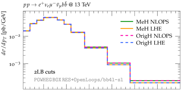
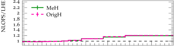
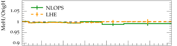
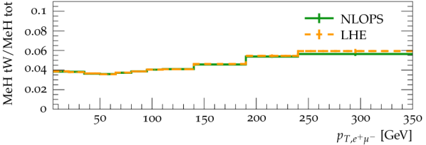
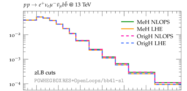
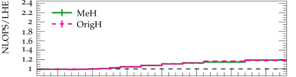
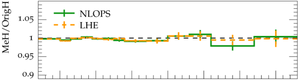
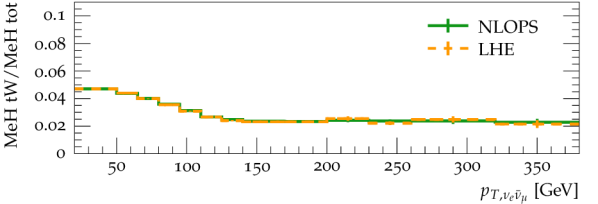
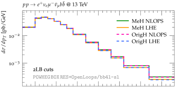
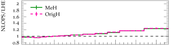
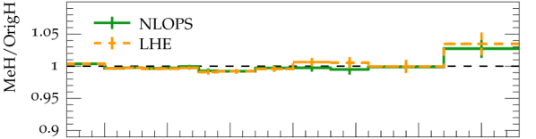
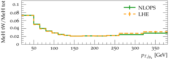
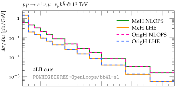
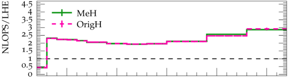
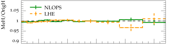
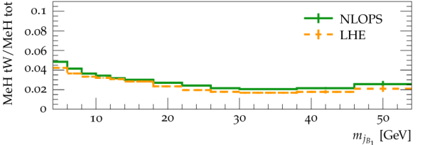
Figure 3: Differential distributions for $pp\to e^{+}\nu_{e}\mu^{-}\bar{\nu}_{\mu}b\bar{b}$ with dilepton+$B$-jet cuts (2LB): comparison of LHE and NLOPS predictions with original (OrigH) vs matrix-element–based (MeH) resonance histories. The lowest frame shows the fraction of events of $tW$ type. See the main text for more details.

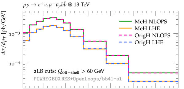
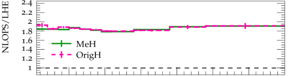
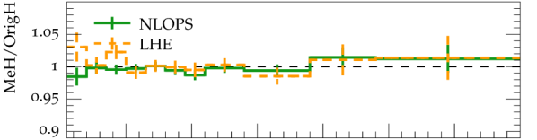
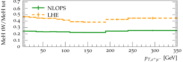
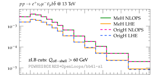
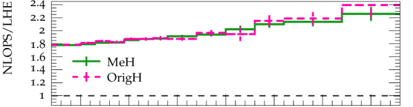
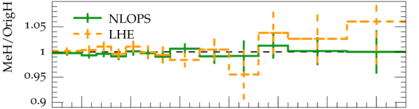
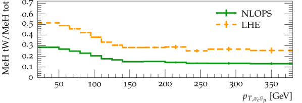
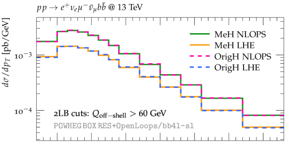
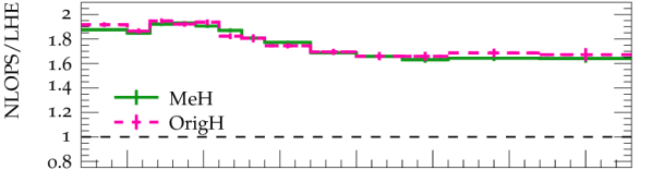
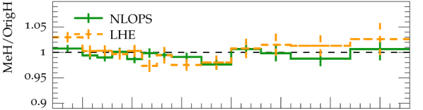
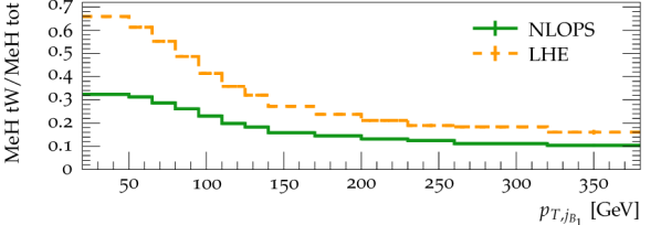
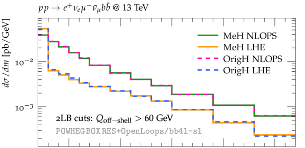
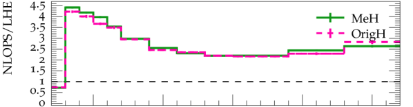
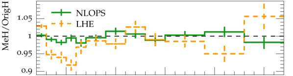
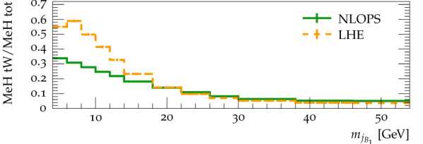
Figure 4: Differential distributions for $pp\to e^{+}\nu_{e}\mu^{-}\bar{\nu}_{\mu}b\bar{b}$ with dilepton+$B$-jet cuts (2LB) and with the additional off-shell cut $Q_{\mathrm{off{\scriptscriptstyle-}shell}}>60\,\text{GeV}$. Same observables and predictions as in Fig. 3.

we investigate the sensitivity of differential distributions to the different definitions of resonance histories. In particular, we consider the distributions in the transverse momentum of the lepton pair and in the missing $p_{\mathrm{T}}$, which feature a significant sensitivity to off-shell effects Denner:2016jyo and may thus be sensitive to the modification of resonance histories. Because the prescription for resonance-history separation directly affects the emission of POWHEG radiation off final-state $b$ partons, depending on whether or not they originate from top decays, we also examine the transverse-momentum and invariant-mass spectra of the hardest $b$ jet.

In Fig. 3 we compare LHE and NLOPS predictions with OrigH and MeH resonance histories in the presence of 2LB cuts. The upper and the lower panels display absolute predictions and various ratios, respectively. The NLOPS/LHE ratio, shown in the second panel, is independent of the choice of the resonance histories, and in the dominant regions of phase space this ratio is close to one, as expected from the sub-percent NLOPS/LHE agreement of the integrated cross sections in Tab. 4. In the tails of the $p_{\mathrm{T}}$ distributions, shower effects are more important and can reach $+20\%$. In the invariant mass of the leading $b$ jet the NLOPS/LHE ratio is around 250%. This can be interpreted as a moderate invariant-mass shift of order 5–10 GeV, which is induced by shower radiation and translates into a large NLOPS/LHE ratio due to the steepness of the distribution in $m_{j_{B_{1}}}$.

The ratio of distributions based on MeH vs OrigH resonance histories, shown in the third panel of Fig. 3, features an exceptional level of agreement, i.e. very small sensitivity to the choice of resonance histories. This holds both at the LHE and NLOPS level, and for all observables, even in the regions where shower effects are sizeable. For each observable, in the fourth panel we show the fraction of events of $tW$ type. This fraction is determined within the MeH approach as the ratio of events with $tW^{-}$ or $\bar{t}W^{+}$ resonance histories with respect to the total. Its kinematic distribution in Fig. 3 shows that, in the 2LB phase space, events of $tW$ type are most abundant in the region where the leading $b$ jet is soft.

In Fig. 4 we present the same distributions applying 2LB cuts and the additional cut $Q_{\mathrm{off{\scriptscriptstyle-}shell}}>60\,\text{GeV}$. As a result of this off-shell cut, the fraction of $tW$ events increases by about a factor eleven (six) and LHE (NLOPS) level, while its kinematic dependence is qualitatively similar as in the full 2LB phase space. The off-shell cut enhances also shower effects, and the NLOPS/LHE ratio can reach a factor two in the tails of the $p_{\mathrm{T}}$ distributions. As discussed above, this enhancement can be attributed to a shower-induced migration of events across the off-shell cut at $Q_{\mathrm{off{\scriptscriptstyle-}shell}}=60\,\text{GeV}$. This interpretation is supported by the fact that the NLOPS/LHE ratio grows with the $p_{\mathrm{T}}$ of the leading $b$ jet, and in the $p_{\mathrm{T},j_{B_{1}}}$ tail the ratio of $t\bar{t}$ over $tW$ events almost doubles when the parton shower is switched on.

For what concerns the effect of resonance histories, we observe that the ratio of MeH/OrigH distributions is mostly consistent with one within statistics. The only significant exception is observed in the small invariant-mass region of the $m_{j_{B_{1}}}$ distribution, where MeH based predictions are up to 7% below OrigH based ones. This effect can be attributed to the different OrigH/MeH treatment of POWHEG radiation in events of $tW$ kind. As discussed above, this OrigH/MeH difference is expected to be mitigated by the parton shower, which is indeed what we observe at NLOPS level. This interpretation is confirmed by the fact that the effect at hand shows up in the $m_{j_{B_{1}}}$ region with the highest fraction of $tW$ events (see the fourth panel). As expected, the observed differences at LHE level are strongly mitigated when the parton shower is switched on. Indeed, at NLOPS level no statistically significant MeH/OrigH difference is observed.

In general, the high level of agreement between MeH vs OrigH resonance histories demonstrates that the ambiguity associated with the choice of resonance-history projectors represents a very small source of uncertainty. This finding inspires further confidence in the POWHEG–RES method. Moreover, the observed agreement can be regarded as a validation of our implementation of the new matrix-element based separation of resonance histories.

8 Comparison of dileptonic and semileptonic channels

In this section we discuss predictions of the new bb4l-sl generator for the semileptonic (SL) process

$$pp \to e^{+}\nu_{e}d{\bar{u}}b\bar{b}\,,$$ (92)

and compare them to predictions of the bb4l-dl generator for the related dilepton (DL) process

$$pp \to e^{+}\nu_{e}\mu^{-}\bar{\nu}_{\mu}b\bar{b}\,,$$ (93)

using the new matrix-element–based resonance histories throughout. The above processes are both dominated by a common $pp\to W^{+}W^{-}b\bar{b}$ subprocess with a $W^{+}\,\to\,e^{+}\nu_{e}$ leptonic decay, and the only difference lies in the hadronic or leptonic nature of the $W^{-}$ decay,

$$W^{-}\,\to\,\mu^{-}\bar{\nu}_{\mu}\qquad\mbox{or}\qquad W^{-}\,\to\,d\bar{u}\,.$$ (94)

More precisely, upon identification of the leptonic and hadronic $W^{-}$ decay products, the two processes are perfectly equivalent at Born level, while all differences arise from the breaking of the trivial correspondence between hadronic and leptonic $W^{-}$ decays, which results from QCD radiation effects in hadronic $W$ decays. Thus, depending on whether a given observable is weakly or strongly sensitive to such QCD effects, the comparison of bb4l-sl and bb4l-dl is expected to yield, respectively, good agreement or sizeable differences. The former case provides a check of the mutual consistency of the two generators, while the latter case can be exploited to gain instructive insights into the origin and the manifestation of QCD radiation effects in various observables. With these two objectives in mind, in the following we define physics objects and observables in a way that enables switching between the cases of weak and strong sensitivity to QCD effects that originate from the fragmentation of jets and/or form their contamination through other sources of QCD radiation.

8.1 Physics objects, $\boldsymbol{W}$ reconstruction and event selection

In this section we define selection cuts and observables that are designed such as to enable a consistent comparison of the SL and DL processes (92)–(93). In particular, we define optimised $W$-reconstruction procedures that are based on MC truth and maximise the correspondence between hadronic and leptonic $W$-boson decays by minimising the sensitivity of the former to QCD radiation effects. Such optimised $W$-boson reconstructions will be enabled and disabled in order to maximise the consistency of bb4l-sl and bb4l-dl predictions for validation purposes and, alternatively, to gain insights into the origin and behaviour of QCD radiation effects.

Physics objects and raw reconstruction of $W$ bosons

Light jets are defined with the anti-$k_{\mathrm{T}}$ algorithm with $R=0.5$. The leptons, neutrinos and $B$ jets are defined as in Sect. 7.1, and in this Section the labels $j_{b}$ and $j_{\bar{b}}$ are used for the leading $b$ and $\bar{b}$ jets.

Leptonic and hadronic $W$-boson decays are reconstructed as follows. In the DL and SL channels, the leptonic $W^{+}\to e^{+}\nu_{e}$ and $W^{-}\to\mu^{-}\bar{\nu}_{\mu}$ decays are reconstructed based on the particle identity and exact four-momenta of their decay products according to MC truth. In the SL channel, the hadronic $W^{-}\to d\bar{u}$ decays are required to form two separate jets, which are labelled as $j_{d}^{W}$ and $j_{\bar{u}}^{W}$. The associated $W^{-}$ bosons are reconstructed by identifying and combining such $j_{d}^{W}$ and $j_{\bar{u}}^{W}$ jets at MC truth level. In the following, this procedure will be referred to as raw $W$ reconstruction.

Recombination and decontamination of hadronic $W$ bosons

At the Born level, the reconstructed hadronic $W^{-}$ boson in the SL channel is equivalent to the leptonic $W^{-}$ boson in the SL channel. However, this simple correspondence can be largely obscured by the effect of QCD radiation and jet clustering. In particular, the hadronic $W^{-}$ mass peak is expected to be smeared as compared to the leptonic one. This is because the $W$ virtuality can be either enlarged, if radiation from outside of $W^{-}$ gets clustered together with $j_{d}^{W}$ and $j_{\bar{u}}^{W}$, or reduced, if the radiation from within $W^{-}$ escapes the cones of $j_{d}^{W}$ and $j_{\bar{u}}^{W}$. In order to restore a high degree of similarity between $W^{-}$ bosons of leptonic and hadronic type, in the following we introduce a recombination and decontamination procedure that minimises the effects of QCD radiation and jet clustering in the reconstruction of hadronic $W^{-}$ bosons.

Recombination of hadronic $W^{-}$ bosons — The fragmentation of $j_{d}^{W}$ and $j_{\bar{u}}^{W}$ jets can lead to a significant reduction of the invariant mass of the reconstructed $W^{-}$ boson. To avoid this effect, based on MC truth we add to $j_{d}^{W}$ and $j_{\bar{u}}^{W}$ all missing partons that originate form the $W^{-}\to d\bar{u}$ decay via NLO radiation or parton showering. Such partons are assigned each to the jet $j_{d}^{W}$ or $j_{\bar{u}}^{W}$ with the smallest $\Delta R$ distance. This $W$ recombination applies also to partons that are clustered into $b$ jets, i.e. together with $W$-recombination we apply a $B$-decontamination procedure, which consists of removing from $B$ jets all gluons and quarks that originate from the $W^{-}\to d\bar{u}$ decay. These corrections are expected to suppress DL–SL differences in the $W^{-}$-mass distribution below the peak as well as in the efficiency of cuts and in distributions involving $j_{d}^{W}$, $j_{\bar{u}}^{W}$ and $B$ jets.

Decontamination of hadronic $W^{-}$ bosons — The clustering of QCD radiation originating from other parts of the process into $j_{d}^{W}$ and $j_{\bar{u}}^{W}$ can significantly increase the invariant mass of the reconstructed $W^{-}$ boson. To avoid this effect, based on MC truth we remove from $j_{d}^{W}$ and $j_{\bar{u}}^{W}$ all partons that do not originate from the $W^{-}\to d\bar{u}$ decay. This $W$-decontamination is combined with a $B$-recombination procedure, where all partons that were removed from $j_{d}^{W}$ and $j_{\bar{u}}^{W}$ are added to the $j_{B}$ jet that is closest in $\Delta R$ if $\Delta R<0.5$. These corrections are expected to suppress DL–SL differences in the $W^{-}$ mass distribution above the peak, as well as in the efficiency of cuts and in distributions involving $j_{d}^{W}$, $j_{\bar{u}}^{W}$ and $B$ jets.

The combination of these recombination and decontamination procedures amounts to an approximate reconstruction of the original hard $d$ and $\bar{u}$ quarks before the emission of any radiation in the $W^{-}$ decay. Thus it is expected to yield a good correspondence between leptonic and hadronic $W$ decays. Again, we note that the purpose of these idealised recombination and decontamination procedures is to investigate QCD radiation patterns in a systematic way.

Acceptance cuts

After the above physics object identification and $W$-reconstruction procedures, and before imposing acceptance cuts, we require that the four objects stemming from $W$-boson decays, i.e. $e^{+}\nu_{e}$ and $\mu^{-}\bar{\nu}_{\mu}$ or $j^{W}_{d}j^{W}_{\bar{u}}$, are pairwise separated by $\Delta R>0.5$. Furthermore, we identify the leading $j_{b}$ and $j_{\bar{b}}$ jets, which are required to be two individual jets, i.e. separated by a distance $\Delta R>0.5$. In addition, we require that $j_{b}$ and $j_{\bar{b}}$ are at a distance $\Delta R>1$ from the four objects stemming from the decay of the $W^{+}$ and $W^{-}$ bosons.

At this stage we count the number $N_{B}$ of jets of type $j_{B}$ with $p_{\mathrm{T}}>25\,\text{GeV}$ and $\eta<2.5$, and we split the phase space in two complementary regions with $N_{B}=1$ and $N_{B}\geq 2$. Finally, we apply one of the following two selections, which require the presence within acceptance cuts of three physics objects corresponding either to a top or an anti-top decay.

$W^{+}b$ selection — We require that the leading $j_{b}$ and the $W^{+}$ decay products, i.e. $e^{+}$ and $\nu_{e}$, fulfill $p_{\mathrm{T}}>25\,\text{GeV}$ and $\eta<2.5$. These three physics objects represent a “top candidate”.

$W^{-}\bar{b}$ selection — We require that the leading $j_{\bar{b}}$ and the $W^{-}$ decay products, i.e. $\mu^{-}$ and $\bar{\nu}_{\mu}$ ($j^{W}_{d}$ and $j^{W}_{\bar{u}}$) in the DL (SL) sample, fulfill $p_{\mathrm{T}}>25\,\text{GeV}$ and $\eta<2.5$. These three physics objects represent an “anti-top candidate”.

8.2 Results

In the following we present comparisons of bb4l predictions in the DL and SL channels for a $W^{+}b$ and a $W^{-}\bar{b}$ selection in the regions with $N_{B}=1$ and $N_{B}\geq 2$. These comparisons are carried out at the LHE level, i.e. focussing on the effect of the hardest POWHEG emissions.

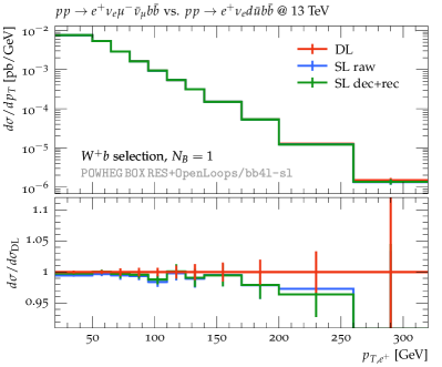
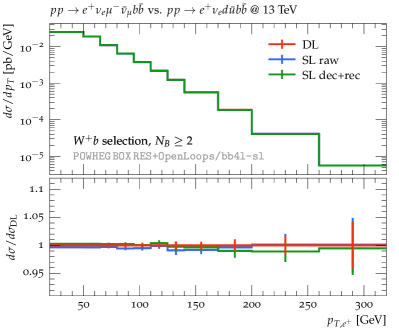
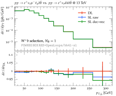
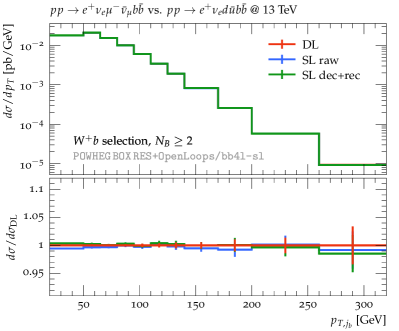
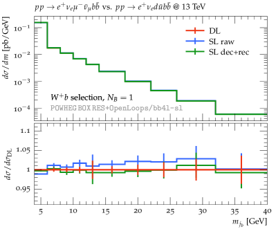
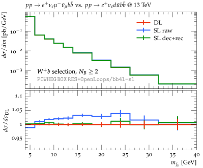
Figure 5: Comparison of bb4l LHE predictions in the dilepton channel (DL) and in the single-lepton channel with naive $W$-reconstruction (SL raw) or with $W$-decontamination and -recombination corrections (SL dec+rec). The distributions in the $p_{\mathrm{T}}$ of the positron and in the $p_{\mathrm{T}}$ and the mass of the leading $b$-jet are compared in the $W^{+}$ phase space with $N_{B}=1$ (left column) and $N_{B}\geq 2$ (right column). See more details in the main text.

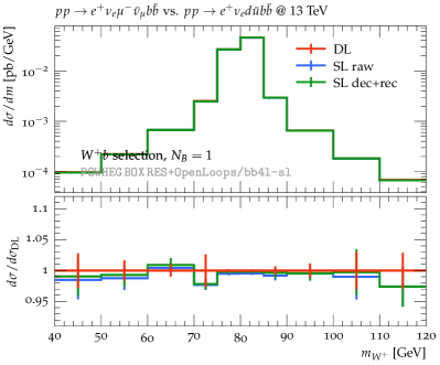
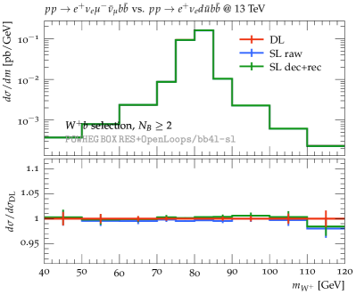
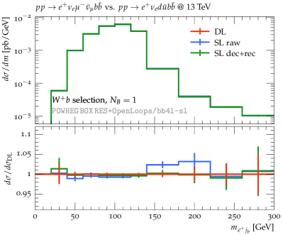
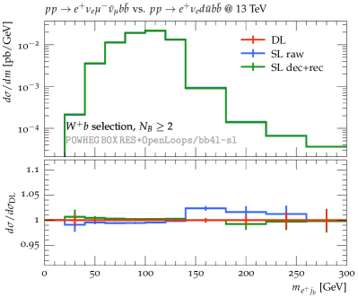
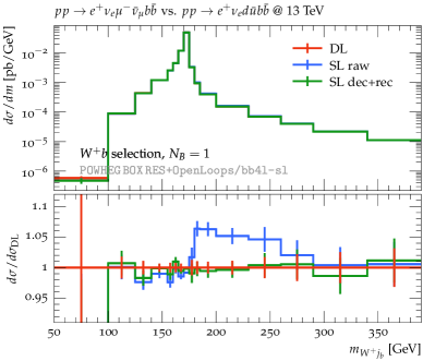
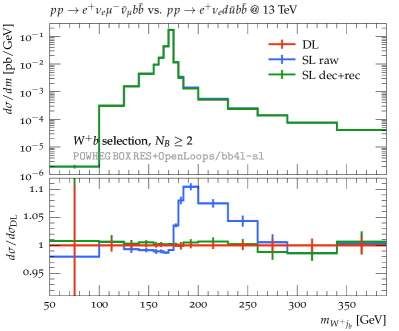
Figure 6: Same comparison as in Fig. 5 for the invariant masses of the reconstructed $W^{+}$ boson, i.e. $m_{W^{+}}=m_{e^{+}\nu_{e}}$, and the invariant masses of the $e^{+}j_{\bar{b}}$ and $W^{+}j_{\bar{b}}$ systems. See more details in the main text.

In Figs. 5–6 we apply a $W^{+}b$ selection and we study various observables that depend on the constituents of the “leptonic top candidate” $e^{+}\nu_{e}j_{b}$. In general, since these three objects are treated in the same way in bb4l-dl and bb4l-sl, we expect to observe good agreement. In fact, in the first five observables of Figs. 5–6 the difference between DL and SL predictions with raw $W$ reconstruction (SL raw) never exceeds 2–3%. This holds both in the $N_{B}=1$ and $N_{B}\geq 2$ phase space. Such small differences are due to the interplay of QCD radiation from hadronic $W^{-}$ decays with the $B$ jets that enter the acceptance cuts or the observables at hand. This is confirmed by the fact that the maximum DL–SL difference goes down to 1% when the $W$-decontamination and -recombination corrections (DL dec+rec) are applied. This reduction is clearly visible in the $j_{b}$ mass distribution, where the 2–3% excess in the SL raw prediction is due to radiation stemming from the hadronic $W$-boson decay, which gets clustered into $j_{b}$ increasing its invariant mass. A similar behaviour is observed in the distribution in $m_{e^{+}j_{b}}$.

As for the distributions in $p_{\mathrm{T},e^{+}}$,  $p_{\mathrm{T},j_{b}}$ and $m_{W^{+}}$, we observe that SL raw predictions are already in excellent agreement with DL ones. Applying the dec+rec corrections this agreement persists. Finally, in the invariant mass of the reconstructed top quark in Fig. 6 we see that SL raw predictions exceed DL ones by up to 10% in the resonance region. This excess reflects a migration of events from the Breit–Wigner peak towards higher invariant mass, which is due to radiation from the hadronic $W^{-}$ decay that gets clustered into $j_{b}$. Similarly as for the $m_{j_{b}}$ distribution, this effect disappears when the dec+rec corrections are applied.

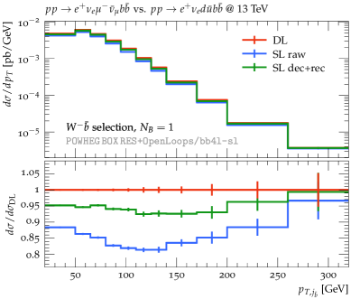
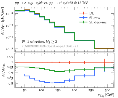
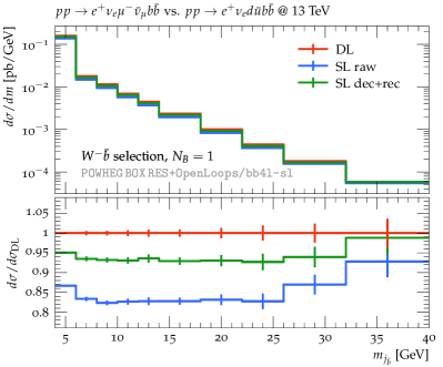
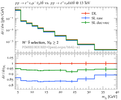
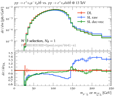
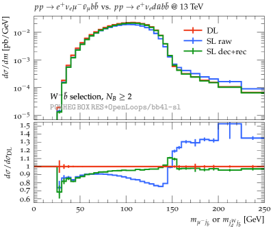
Figure 7: Comparison of bb4l LHE predictions in the the dilepton channel (DL) and in the single-lepton channel with raw $W$-reconstruction (SL raw) or with $W$-decontamination and -recombination corrections (SL dec+rec). The distributions in the $p_{\mathrm{T}}$ and the mass of the leading $B$-jet and in the mass of the $\mu^{-}j_{b}$ (DL channel) or $j_{d}j_{b}$ (SL channel) systems are compared in the $W^{+}$ phase space with $N_{B}=1$ (left column) and $N_{B}\geq 2$ (right column).

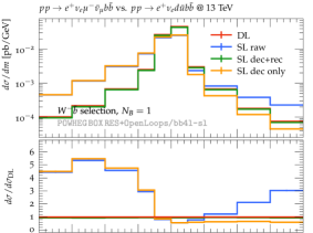
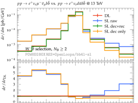
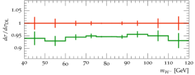
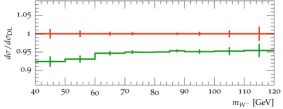
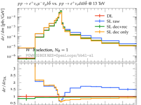
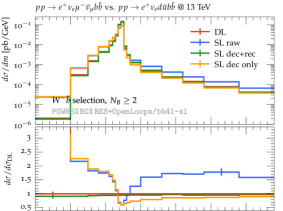
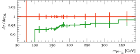
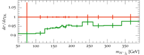
Figure 8: Similar comparison as in Fig. 7 for the distributions in the invariant masses of the reconstructed $W^{-}$ bosons, which correspond either to the $\mu^{-}\bar{\nu}_{\mu}$ or the $j^{W}_{d}j^{W}_{\bar{u}}$ systems, and of the associated $W^{-}j_{b}$ systems. Here in addition to DL, SL raw and SL dec+rec we also show predictions in the single-lepton channel with only $W$-decontamination (SL dec only). The central frame shows the various DL/SL ratios, while the lower frame shows the ratio of SL dec+rec wrt DL with higher resolution.

In Figs. 7–8 we apply a $W^{-}\bar{b}$ selection and we study various observables that depend on the constituents of the $j^{W}_{d}j^{W}_{\bar{u}}j_{\bar{b}}$ hadronic “anti-top candidate” in the SL channel and its $\mu^{+}\bar{\nu}_{\mu}j_{\bar{b}}$ leptonic counterpart in the DL channel. In Fig. 7 we show the distributions in the $p_{\mathrm{T}}$ and the mass of $j_{\bar{b}}$ as well as the invariant mass of the $\mu^{-}j_{\bar{b}}$ ($j^{W}_{d}j_{\bar{b}}$) pair in the DL (SL) channel. In general, due to the presence of hadronic $W^{-}$ decays, in the $W^{-}\bar{b}$ selection we observe much more pronounced DL–SL differences as compared to the $W^{+}b$ selection. In the bulk of all distributions, SL raw predictions feature a deficit of about 10-20% wrt the DL channel. This effect can be attributed to the fragmentation of light jets from $W^{-}$ decays, which leads to reduced $p_{\mathrm{T}}$ as compared to the decay products of the leptonic $W^{-}$ decay, and thus to fewer events passing the acceptance cuts in the SL channel. In the tail of the $j^{W}_{d}j_{\bar{b}}$ mass distribution, above the edge that is located around 150 GeV, we observe the opposite behaviour, i.e. an excess of SL raw events as compared to DL ones. This can be attributed to the migration of SL events across the edge as a result of large-angle QCD radiation that is emitted by the $W^{-}$ decay and absorbed by $j_{\bar{b}}$. When applying dec+rec corrections, all DL–SL differences are largely suppressed as expected. More precisely, with the only exception of the suppressed region of small $j^{W}_{d}j_{\bar{b}}$ invariant mass, the remaining DL–SL difference is at the level of 5–8%. This residual mismatch can be attributed to imperfections of the dec+red corrections, such as the ambiguity in the assignment of large-angle QCD radiation to the individual $j^{W}_{d}$ or $j^{W}_{\bar{u}}$ jets.

In Fig. 8 we present the same comparison for the distributions in the invariant masses of the reconstructed $W^{-}$ boson and of the anti-top quark. In these observables, the DL–SL differences due to the kinematic effects of QCD radiation and jet clustering are strongly amplified by the presence of narrow Breit–Wigner peaks. In the $N_{B}=1$ and $N_{B}\geq 2$ regions, and for both invariant-mass distributions, the SL raw predictions feature huge enhancements in the off-shell regions on both sides of the resonances. Such enhancements are due to two opposite mechanisms, where resonant events lose invariant mass due to the fragmentation of the $j^{W}_{d}$ or $j^{W}_{\bar{u}}$ jets or, alternatively, gain invariant mass due to QCD radiation that does not originate from the hadronic $W^{-}$ but is clustered into the $j^{W}_{d}$ or $j^{W}_{\bar{u}}$ jets. The light-jet clustering mechanism can be reversed by applying the $W$-decontamination correction (see “SL dec only” curves). As a result, in the high-mass tails the SL excesses of up to 100–200% disappear, and the SL cross section goes down to around 10–30% below the DL one. This deficit can be attributed to the light-jet fragmentation mechanism, which is also responsible for the huge DL excesses below the Breit–Wigner peaks. These remaining DL–SL differences are strongly suppressed when the $W$-decontamination is supplemented by the $W$-recombination correction (SL dec+rec). In this case, in the $W$-mass distribution the shape of DL and SL predictions become almost identical, and in a broad region around the Breit–Wigner peaks we observe a rather constant difference around 5%, similarly as in Fig. 7. An equally good shape agreement and 5% difference is observed also in the anti-top mass distributions.

In summary, the results of Figs. 5–8 demonstrate the mutual consistency of the bb4l-dl and bb4l-sl versions of the bb4l generator, providing also a qualitative and quantitative picture of the jet-fragmentation and jet-clustering effects that are responsible for the expected differences between DL and SL channels.

9 Shower effects and comparison against on-shell $t\bar{t}+tW$ generators

In this section we turn our interest in the investigation of $t\bar{t}+tW$ production with semileptonic decays to the parton shower, and we quantify its effect by comparing bb4l-sl predictions at the LHE and NLO+PS levels. Moreover we compare the bb4l-sl generator against the well established POWHEG generators that describe $t\bar{t}$ and $tW$ production in the on-shell approximation, namely the hvq Frixione:2007vw and the ${\tt ST}_{\tt wtch}$ Re:2010bp generators. This comparison provides quantitative information on various physics ingredients—such as off-shell and interference effects—that are included at NLO+PS accuracy in bb4l-sl, while in hvq+${\tt ST}_{\tt wtch}$ they are either absent, or only included at LO+PS accuracy.

9.1 Differences between on-shell and off-shell generators

As a basis for the comparison of on-shell against off-shell POWHEG generators for $t\bar{t}+tW$ production with semileptonic decays, in the following we list the main deficits of hvq+${\tt ST}_{\tt wtch}$ wrt bb4l-sl in terms of physics ingredients and perturbative accuracy.

• In bb4l-sl, all $t\to Wb$ and $W\to q\bar{q}^{\prime}$ decays are NLO+PS accurate, i.e. the hardest emission is based on matrix elements, while in hvq+${\tt ST}_{\tt wtch}$ such decays are only LO+PS accurate, i.e. QCD radiation is entirely generated by the parton shower. The resulting differences can be quite sizeable at the LHE level. However, after parton showering they tend to be rather small. This is due to fact that shower emissions in $t\to Wb$ and $W\to q\bar{q}^{\prime}$ decays are systematically improved through matrix-element corrections (MEC) in Pythia.

• The ${\tt ST}_{\tt wtch}$ generator describes $tW$ production as a $gb\to tW$ hard process with massless $b$ quarks. This implies that $tW$ contributions to the phase space with two resolved $b$ jets arise via $pp\to tWb$ real-emission channels and are only LO+PS accurate. In contrast, in bb4l-sl $b$-quark mass effects are included throughout, and $tW$ contributions are NLO+PS accurate in the whole phase space with up to two resolved $b$ jets.

• In bb4l-sl the $t\bar{t}$–$tW$ interference is entirely included at NLO+PS accuracy, while the ${\tt ST}_{\tt wtch}$ generator supports two different treatments of the interference. In the diagram-subtraction approach (${\tt ST}_{\tt wtch}$-$\tt{DS}$), the interference is included in the $pp\to tWb$ real-emission processes, i.e. with LO+PS accuracy, while in the diagram-removal approach (${\tt ST}_{\tt wtch}$-$\tt{DR}$) it is omitted. Thus, the difference between ${\tt ST}_{\tt wtch}$-$\tt{DR}$ and ${\tt ST}_{\tt wtch}$-$\tt{DS}$ can be regarded as a LO+PS estimate of the $t\bar{t}$–$tW$ interference.

• In bb4l-sl non-resonant effects, i.e. contributions from diagrams that are free from $t\to bW$ sub-topologies, are included throughout at NLO+PS accuracy, while in hvq+${\tt ST}_{\tt wtch}$ they are entirely absent.

• Off-shell effects are exact in bb4l-sl, while the hvq+${\tt ST}_{\tt wtch}$ generators employ matrix elements with on-shell top quarks together with an approximate treatment of off-shell effects, which consists of re-distributing the invariant masses of top quarks (and their decay products) according to a Breit–Wigner distribution.

	bb4l-sl	hvq+${\tt ST}_{\tt wtch}$-$\tt{DS}$	hvq+${\tt ST}_{\tt wtch}$-$\tt{DR}$
$t\to Wb$ and $W\to q\bar{q}^{\prime}$ decays	NLO+PS	LO+PS	LO+PS
$tWb$ production	NLO+PS	LO+PS	LO+PS
$t\bar{t}$–$tW$ interference	NLO+PS	-	LO+PS
off-shell effects	NLO+PS	approx.	approx.
non-resonant contributions	NLO+PS	-	-

Table 5: Summary of the main differences—in terms of physics ingredients and their formal accuracy—between bb4l and the hvq+${\tt ST}_{\tt wtch}$ generators for the cases where ${\tt ST}_{\tt wtch}$ is applied in diagram-subtraction (${\tt ST}_{\tt wtch}$-$\tt{DS}$) or diagram-removal (${\tt ST}_{\tt wtch}$-$\tt{DR}$) mode (see the discussion in Sect. 9.1). The indicated formal accuracy, NLO+PS or LO+PS, refers to the phase space with two resolved $b$ jets.

The above differences between hvq+${\tt ST}_{\tt wtch}$ and bb4l-sl are summarised in a schematic way in Tab. 5.

9.2 Physics objects and event selection

The comparisons presented in the following subsections are based on a semi-realistic event selection that is inspired by experimental analyses of $t\bar{t}$ production. In particular, as described in the following, we focus on semileptonic $t\bar{t}$ signatures with two resolved $b$ jets.

Physics objects and cuts — The event selection consists of the following steps.

• Based on MC truth we identify the charged lepton and the neutrino stemming from the decay of the $W^{+}$ boson. For both we require $p_{\mathrm{T}}>25\,\text{GeV}$, and in the case of the charged lepton also $|\eta|<2.5$.

• Jets are built using the anti-$k_{\mathrm{T}}$ algorithm with $R=0.5$ and are categorised into $b$ jets, $\bar{b}$ jets and light jets depending on the presence of $b$ quarks among their constituents at MC-truth level.

• We require (at least) two light jets, plus one $b$ jet and one $\bar{b}$ jet with $p_{\mathrm{T}}>25\,\text{GeV}$ and $|\eta|<2.5$. In the following the label $j_{b}$ ($j_{\bar{b}}$) is used to denote the leading $b$ ($\bar{b}$) jet within acceptance.

Reconstruction of resonances—Certain observables are defined in terms of the $W$-boson and top-quark momenta, which are reconstructed as follows.

• The momentum of the leptonically decaying $W$ boson is defined as the sum of the four-momenta of the corresponding lepton and neutrino (also when $|\eta_{\nu}|>2.5$).

• To reconstruct the hadronic $W$ boson we consider the four hardest light jets within acceptance and we select the combination of 2 or 3 light jets whose invariant mass is closest to $m_{W}$.

• The (anti-)top-quark momentum is reconstructed as the sum of the momenta of the reconstructed ($W^{-}$) $W^{+}$ boson, plus the ($j_{\bar{b}}$) $j_{b}$ jet and up to one of the remaining light jets within acceptance. The latter is included in case it yields an invariant mass closer to $m_{t}$.

9.3 Integrated cross section

		inclusive phase space		$e^{+}\nu_{e}bbjj$ fiducial phase space
				$R=0.5$		$R=0.2$
		$\sigma$[pb]	$\frac{\sigma}{\phantom{\big{|}}\sigma_{{\tt bb4l-sl}}^{\mathrm{NLOPS}}}$	$\sigma$[pb]	$\frac{\sigma}{\phantom{\big{|}}\sigma_{{\tt bb4l-sl}}^{\mathrm{NLOPS}}}$	$\sigma$[pb]	$\frac{\sigma}{\phantom{\big{|}}\sigma_{{\tt bb4l-sl}}^{\mathrm{NLOPS}}}$
bb4l-sl	NLOPS	57.56(2)	1	16.30(1)	1	14.639(9)	1
bb4l-sl	LHE	57.56(2)	1	16.33(1)	1.002	17.17(1)	1.173
hvq	NLOPS	54.340(9)	0.944	15.910(6)	0.976	14.244(6)	0.973
hvq	LHE	54.339(9)	0.944	17.446(7)	1.070	18.614(8)	1.272
${\tt ST}_{\tt wtch}$-$\tt{DR}$	NLOPS	2.5524(3)	0.044	0.5249(2)	0.032	0.4683(2)	0.032
${\tt ST}_{\tt wtch}$-$\tt{DR}$	LHE	2.5524(3)	0.044	0.3082(1)	0.019	0.3470(1)	0.024
${\tt ST}_{\tt wtch}$-$\tt{DS}$	NLOPS	2.5194(3)	0.044	0.4877(2)	0.030	0.4232(2)	0.029
${\tt ST}_{\tt wtch}$-$\tt{DS}$	LHE	2.5194(3)	0.044	0.3002(1)	0.018	0.3280(1)	0.022
hvq + ${\tt ST}_{\tt wtch}$-$\tt{DR}$	NLOPS	56.892(8)	0.988	16.475(6)	1.011	14.780(6)	1.010
hvq + ${\tt ST}_{\tt wtch}$-$\tt{DR}$	LHE	56.893(8)	0.988	17.754(7)	1.089	18.961(7)	1.295
hvq + ${\tt ST}_{\tt wtch}$-$\tt{DS}$	NLOPS	56.859(8)	0.988	16.398(6)	1.006	14.667(6)	1.002
hvq + ${\tt ST}_{\tt wtch}$-$\tt{DS}$	LHE	56.858(8)	0.988	17.746(7)	1.089	18.942(7)	1.294

Table 6: Cross sections for $pp\to e^{+}\nu_{e}jjb\bar{b}$ at 13 TeV in the fully inclusive phase space (columns 3–4) and in the fiducial phase space with two $b$ jets plus two light jets, a lepton and a neutrino, as defined in Sect. 9.2 (columns 5–8). In the latter case we compare results based on the anti-$k_{\mathrm{T}}$ algorithm with $R=0.5$ (columns 5–6) and $R=0.2$ (columns 7–8). The various rows report bb4l-sl predictions at the LHE and NLO+PS level, as well as corresponding hvq+${\tt ST}_{\tt wtch}$-$\tt{DR}$ and hvq+${\tt ST}_{\tt wtch}$-$\tt{DS}$ predictions. In the case of bb4l-sl, by default all LHE and NLOPS results include the inverse-width expansion discussed in Sect. 3. In this comparison all input parameters, QCD scales, PDFs and branching ratios are chosen consistently with the setup described in Sect. 6.

Cross sections obtained with the bb4l-sl and hvq+${\tt ST}_{\tt wtch}$ generators at LHE and NLOPS levels are reported in Tab. 6. Let us first focus on fully inclusive cross sections. In this case, as expected from the unitarity of NLO+PS matching, LHE and NLOPS predictions coincide with each other and correspond exactly to fixed-order NLO. As compared to bb4l-sl, the hvq inclusive cross section features a deficit of 5.6%, which is mainly due to the missing $tW$ contribution. The latter amounts to 4.4% of the bb4l-sl cross section, both in the DR and DS approach, which points to a very small $t\bar{t}$–$tW$ interference. The combined hvq+${\tt ST}_{\tt wtch}$ prediction lies only 1.2% below bb4l-sl. This small difference can be attributed to bottom-mass effects, off-shell and non-resonant contributions of $\mathcal{O}(\Gamma_{t}/m_{t})$, or to effects that originate from $\mathcal{O}(\alpha_{\rm S}^{2})$ differences in the treatment of bottom-loop contributions to the gluon-PDF, and in the perturbative expansion of $1/\Gamma_{t}$. In this respect we note that the consistent expansion of $1/\Gamma_{t}$ terms up to $\mathcal{O}(\alpha_{\rm S})$, as described in Sect. 3, is mandatory in order to achieve percent-level agreement between hvq+${\tt ST}_{\tt wtch}$ and bb4l-sl. In particular, we have checked that omitting the inverse-width expansion (55)–(56) in bb4l-sl yields

$$\frac{\sigma_{\tt bb4l-sl}}{\sigma_{\tt hvq+ST}}\Bigg{|}_{\mbox{\scriptsize no $1/\Gamma_{t}$ expansion }}=\;1.074\,,$$ (95)

which corresponds to a difference bigger than the entire $tW$ contribution. Based on the analysis of Sect. 3, it is clear that a similarly large mismatch would show up also in fiducial cross sections and differential observables.

Moving to the $e^{+}\nu_{e}bbjj$ fiducial phase space, we observe that the bb4l-sl cross section remains largely independent of shower effects. More precisely, when jet cuts are applied using the standard jet resolution, $R=0.5$, the difference between NLOPS and LHE predictions are at the permil level. This tiny sensitivity to parton showering is mainly due to the fact that, in bb4l-sl, the hardest QCD emissions from all top-production and -decay subprocesses are entirely controlled by matrix elements. This is not the case for hvq and ${\tt ST}_{\tt wtch}$, where QCD radiation in top decays is entirely generated by the parton shower. Moreover, in the case of ${\tt ST}_{\tt wtch}$ also the hardest radiation on top of the $pp\to tWb$ production process is entirely due to the shower. In the fiducial hvq cross section such shower effects are around $-10\%$ and are most likely dominated by negative jet-$p_{\mathrm{T}}$ shifts resulting from jet fragmentation. As for the ${\tt ST}_{\tt wtch}$ fiducial cross section, we observe that parton showering shifts the LHE result by about $+65\%$. This large positive effect can be attributed to positive jet-$p_{\mathrm{T}}$ shifts resulting from ISR contamination of hard jets. This interpretation is supported by the fact that the shower sensitivity of the ${\tt ST}_{\tt wtch}$ fiducial cross section is strongly attenuated when the jet resolution is reduced to $R=0.2$, while in the case of hvq its is strongly enhanced. Note that, for $R=0.2$, shower effects become quite significant also in the bb4l-sl fiducial cross section, where they amount to $-15\%$, while their impact in hvq+${\tt ST}_{\tt wtch}$ is around $-23\%$.

Comparing bb4l-sl to hvq+${\tt ST}_{\tt wtch}$ at the NLOPS level, we find that the percent-level agreement observed in the inclusive cross section persists also in the fiducial phase space, both for $R=0.5$ and $R=0.2$. More precisely, when cuts are applied the relative difference wrt bb4l-sl moves form about $-1\%$ to $+1\%$. This level of agreement is remarkable, since the fiducial cross section is sensitive to the modelling of QCD radiation in $tW$ production and top decays, which is entirely controlled by Pythia in hvq+${\tt ST}_{\tt wtch}$. In this respect, we note that Pythia’s matrix-element corrections play a significant role. We have checked that disabling such corrections shifts the fiducial hvq+${\tt ST}_{\tt wtch}$ cross section (for $R=0.5$) by about $-2.5\%$, while in bb4l-sl the effect of Pythia’s matrix-element corrections is at the few-permil level. Finally we note that, in the fiducial region, the DS--DR difference points to interference effects of the order to 10% of the $tW$ contribution, which amounts to only 2–3 permil of the total fiducial cross section.

9.4 Shower effects in differential distributions

In Figs. 9–11 we investigate the impact of shower effects in the bb4l-sl and hvq+${\tt ST}_{\tt wtch}$ generators by comparing LHE and NLOPS predictions for various differential distributions that describe the behaviour of the positron, the leading $b$ and $\bar{b}$ jet, the leptonically decaying $W^{+}$ boson and $t$ quark, as well as the hadronically decaying $W^{-}$ boson and $\bar{t}$ quark. These comparisons are carried out in the $e^{+}\nu_{e}bbjj$ fiducial region, and the decaying $W$ bosons and (anti-)top quarks are reconstructed as detailed in Sect. 9.2.

In the positron-rapidity distribution (Fig. 9(a)) we observe that the NLOPS/LHE ratios for $R=0.5$ and $R=0.2$ are nearly independent of $\eta_{e^{+}}$ and behave as in the case of the fiducial cross section. This holds both for bb4l-sl and hvq+${\tt ST}_{\tt wtch}$. A similarly stable behaviour is observed also in the positron-$p_{\rm T}$ distribution (Fig. 9(b)), but only for moderate $p_{\mathrm{T},e^{+}}$, while above 100 GeV shower effects become increasingly sensitive to $p_{\mathrm{T},e^{+}}$. This behaviour is quite similar in bb4l-sl and hvq+${\tt ST}_{\tt wtch}$. Thus it is probably due to the interplay of ISR with the acceptance cuts, since ISR is handled in a similar way in the different generators.

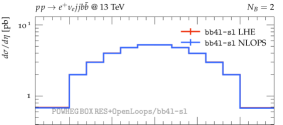
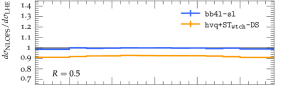
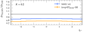
(a)

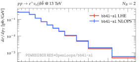
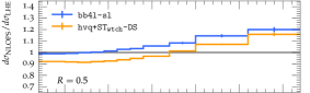
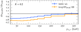
(b)

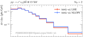
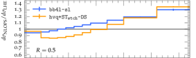
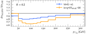
(c)

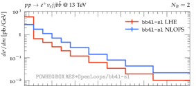
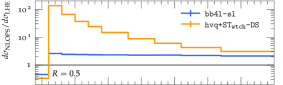
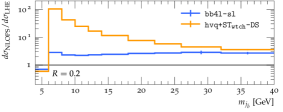
(d)

Figure 9: Impact of the parton shower for $pp\to e^{+}\nu_{e}jjb\bar{b}\,$ at 13 TeV in the fiducial phase space with two $b$-jets plus two light jets, a positron and a neutrino, as defined in Sect. 9.2: distributions in the rapidity of the positron (9(a)), its transverse momentum (9(b)), as well as the transverse momentum of the hardest $\bar{b}$-jet (9(c)) and its invariant mass (9(d)). The upper frame shows LHE and NLOPS predictions of bb4l-sl for $R=0.5$, while the middle (lower) frames compare the NLOPS/LHE ratios of the bb4l-sl and hvq+${\tt ST}_{\tt wtch}$-$\tt{DS}$ generators for $R=0.5$ ($R=0.2$).

The above interpretation is supported by Fig. 9(c), where we observe that the NLOPS/LHE ratios are rather sensitive to the $p_{\mathrm{T}}$ of the hardest $\bar{b}$ jet. In particular, the effect of the shower grows significantly at large $p_{\mathrm{T}}$. We have checked that the corresponding distribution for the case of the hardest $b$ jet behaves in a very similar way.

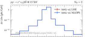
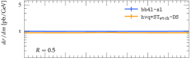
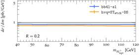
(a)

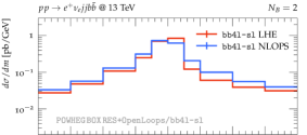
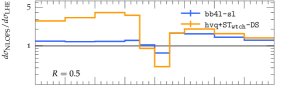
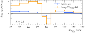
(b)

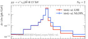
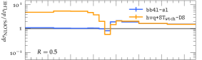
(c)

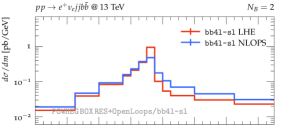
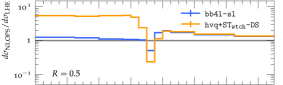
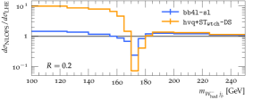
(d)

Figure 10: Distributions in the reconstructed invariant masses of the leptonically decaying $W^{+}$ (10(a)) and hadronically decaying $W^{-}$ boson (10(b)), as well as of the leptonically decaying top (10(c)) and hadronically decaying anti-top quark (10(d)). Same acceptance cuts, predictions and ratios as in Fig. 9.

Also the distributions in the masses of the hardest $b$ and $\bar{b}$ jets behave in a similar way, and in Fig. 9(d) we present the one for the $\bar{b}$ jet. This observable is highly sensitive to the parton shower, and NLOPS/LHE corrections are completely different in bb4l-sl and hvq+${\tt ST}_{\tt wtch}$. The reason is that all bins with $m_{j_{\bar{b}}}>m_{b}$ are mostly populated by QCD radiation off $\bar{b}$ quarks, which is modelled in a different way in the different generators. In the case of hvq+${\tt ST}_{\tt wtch}$, where QCD radiation off $\bar{b}$ quarks is entirely stemming from the parton shower, NLOPS/LHE corrections have a huge impact, which varies between a factor four and a hundred in the plotted region. In contrast, in bb4l-sl, where the hardest emission is controlled by the matrix elements, NLOPS/LHE corrections are around a factor 2–3 and roughly constant.

The distributions in the invariant masses of the reconstructed $W^{+}$ and $W^{-}$ bosons, $m_{W^{+}_{\mathrm{lept}}}$ and $m_{W^{-}_{\mathrm{had}}}$, are shown in Figs. 10(a)–10(b). In the case of the leptonically decaying $W^{-}$, apart from normalisation effects at the level of the fiducial cross section, the invariant-mass distribution is completely insensitive to QCD radiation. In contrast, the modelling of QCD radiation has an important impact on the invariant mass of the hadronically decaying $W^{-}$. Below resonance, shower radiation tends to increase the cross section due to jet-fragmentation processes, where QCD partons escape from the reconstructed $W$ boson. In bb4l-sl such effects are around $20\%$, while in hvq+${\tt ST}_{\tt wtch}$ they reach a factor four. The shower tends to increase the cross section also above the $W^{-}$ resonance. This can be attributed to the contamination of the reconstructed $W^{-}$ boson through ISR or QCD radiation stemming from $b$ quarks. Here the differences between bb4l-sl and hvq+${\tt ST}_{\tt wtch}$ are less dramatic since in both cases the hardest initial-state emission is generated by POWHEG. The above interpretations of shower effects are consistent with the observed dependence on the jet radius: when $R$ is reduced from 0.5 to 0.2, jet-fragmentation effects (below resonance) tend to increase, while jet-contamination effects (above resonance) tend to decrease.

The distributions in the invariant masses of the reconstructed $t\to W^{+}j_{b}$ and $\bar{t}\to W^{-}j_{\bar{b}}$ resonances, $m_{W^{+}_{\mathrm{lept}}\,j_{b}}$ and $m_{W^{-}_{\mathrm{had}}\,j_{\bar{b}}}$, are shown in Figs. 10(c)–10(d). In the case of the $t\to W^{+}j_{b}$ resonance (Fig. 10(c)), in spite of the leptonic nature of the $W^{+}$ decay, we observe qualitatively similar shower effects as for the hadronically decaying $W^{-}$ (Fig. 10(b)). In particular, in hvq+${\tt ST}_{\tt wtch}$ we find sizeable positive shower corrections that tend to increase (decrease) below (above) resonance when $R$ is reduced from 0.5 to 0.2. Since the involved $W^{+}$ boson decays leptonically, this behaviour must be due to fragmentation and contamination processes that involve the associated $b$ jet. We note also that, as compared to hvq+${\tt ST}_{\tt wtch}$, the shower sensitivity of bb4l-sl is much smaller below resonance, while above resonance it is similar. This suggests that $b$-jet contamination is dominated by ISR, which is handled in a similar way in the different generators. Finally, we observe that shower effects in the invariant-mass distribution of the hadronically decaying anti-top quark (Fig. 10(d)) are quite similar as in the case of the leptonically decaying top (Fig. 10(c)). Thus, the sizeable shower corrections to the invariant mass of the hadronic $W^{-}$ (Fig. 10(b)) seem to have little impact on the reconstructed mass of the hadronic anti-top. This is most likely due to the fact that, inside a hadronic $t\to Wb\to jjb$ decay, the radiation that is emitted from the $b$ quark which contaminates the reconstructed hadronic $W$ boson (or vice versa) does not have any impact on the reconstructed top-quark momentum.

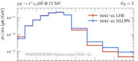
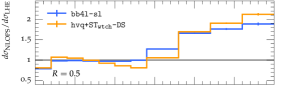
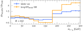
Figure 11: Distribution in the invariant mass $m_{e^{+}j_{b}}$ of the positron and the hardest $b$ jet. Same acceptance cuts, predictions and ratios as in Fig. 9.

Finally, in Fig. 11 we present the distribution in the invariant mass of the positron and the $b$ jet, i.e. the visible decay products of the leptonically decaying top quark. At LO, this observable features a kinematic edge at $m_{e^{+}\,j_{b}}^{2}=m_{t}^{2}-m_{W}^{2}\simeq(152\,\text{GeV})^{2}$, which can be exploited for top-quark mass measurements or in order to design cuts that suppress backgrounds due to on-shell top-quark production. In the region above the edge, which is entirely populated by events with QCD radiation, we observe that bb4l-sl and hvq+${\tt ST}_{\tt wtch}$ are both strongly sensitive to shower radiation. This suggests that the observed NLOPS/LHE corrections are dominated by ISR, which is handled in a similar way in the different generators. In the region below the edge, the impact of the shower is much less pronounced. For $R=0.5$, in hvq+${\tt ST}_{\tt wtch}$ it can reach 20%, while bb4l-sl is largely insensitive to the parton shower.

9.5 Off-shell vs on-shell generators

In Figs. 12–14 we compare predictions of the off-shell bb4l-sl generator and its on-shell counterparts, hvq+${\tt ST}_{\tt wtch}$, for the same set of observables investigated in Sect. 9.4. In addition, in order to quantify the relative importance of the $t\bar{t}$ and $tW$ production modes we also present pure ${\tt hvq}$ results, and to assess $t\bar{t}$–$tW$ interference effects we compare ${\tt ST}_{\tt wtch}$ predictions in diagram-subtraction (DS) and diagram-removal (DR) mode. Moreover, both for bb4l-sl and hvq+${\tt ST}_{\tt wtch}$, we present extra ratios that illustrate the effect of the matrix-element corrections that are applied within Pythia8 when showering top-quark and $W$-boson decays.

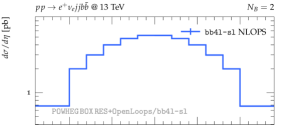
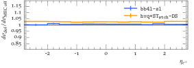
(a)

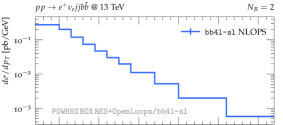
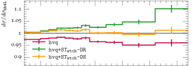
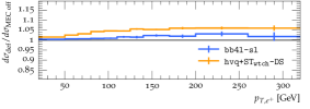
(b)

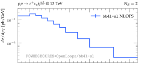
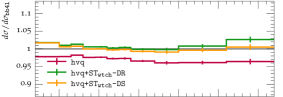
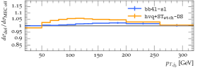
(c)

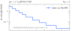
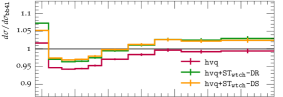
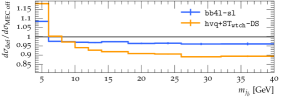
(d)

Figure 12: Comparison of NLOPS predictions of on-shell and off-shell generators for $pp\to e^{+}\nu_{e}jjb\bar{b}\,$ at 13 TeV in the fiducial phase space with two $b$ jets plus two light jets, a positron and a neutrino, as defined in Sect. 9.2: distributions in the rapidity of the positron (12(a)), its transverse momentum (12(b)), as well as the transverse momentum of the hardest $\bar{b}$ jet (12(c)) and its invariant mass (9(d)). The upper frame shows NLOPS predictions of bb4l for $R=0.5$. The middle frame shows ratios wrt bb4l-sl for the case of hvq, hvq+${\tt ST}_{\tt wtch}$ in DS and DR mode, while the lower frame shows the ratio of hvq+${\tt ST}_{\tt wtch}$-$\tt{DS}$ and bb4l-sl distributions obtained with default Pythia settings ($\mathrm{d}\sigma_{\mathrm{def}}$) and disabling Pythia’s matrix-element corrections ($\mathrm{d}\sigma_{{\mathrm{ME\,off}}}$).

In the lepton-rapidity distribution (Fig. 12(a)) all ratios between predictions of bb4l-sl, hvq, hvq+${\tt ST}_{\tt wtch}$-$\tt{DR}$ and hvq+${\tt ST}_{\tt wtch}$-$\tt{DS}$ are nearly constant, and their values are consistent with those observed at the level of the fiducial cross section. This holds also for the distribution in the positron’s transverse momentum (Fig. 12(b)) in the region of moderate $p_{\mathrm{T}}$, while above 100 GeV the DS and DR prescriptions yield increasingly different cross sections pointing to a sizeable $t\bar{t}$–$tW$ interference. For $p_{\mathrm{T},e^{+}}$ around 300 GeV, the pure hvq prediction lies $4\%$ below bb4l-sl, and adding ${\tt ST}_{\tt wtch}$ in DR mode, i.e. the pure $tW$ contribution, shifts the result by $+15\%$, while switching from DR to DS mode, i.e. including the interference, results in a shift of $-9\%$, which brings hvq+${\tt ST}_{\tt wtch}$ in very good agreement with bb4l-sl. When using the DS prescription, the difference between hvq+${\tt ST}_{\tt wtch}$ and bb4l-sl is below 1–2% in the entire plotted range. As demonstrated in the second ratio plot, this excellent consistency is guaranteed also by Pythia’s matrix-element corrections, whose effect at high $p_{\mathrm{T},e^{+}}$ is around $+6\%$ in hvq+${\tt ST}_{\tt wtch}$ and only $+2\%$ in bb4l-sl. In general, in all considered distributions the sensitivity of bb4l-sl to Pythia’s matrix-element corrections is strongly suppressed as compared to hvq+${\tt ST}_{\tt wtch}$. This is expected, since in bb4l-sl such shower corrections affect only the second and subsequent emissions.

Also for the distribution in the $p_{\mathrm{T}}$ of the hardest $\bar{b}$ jet, shown in Fig. 12(c), we find agreement at the few-percent level between hvq+${\tt ST}_{\tt wtch}$-$\tt{DS}$ and bb4l-sl. Here the most significant deviation shows up in the first bin and amounts to only 2%. The relative weight of $tW$ grows from 2% at low $p_{\mathrm{T}}$ to about 4% in the tail, while Pythia’s matrix-element corrections in hvq+${\tt ST}_{\tt wtch}$ vary between $+2\%$ and -$5\%$ depending on the $p_{\mathrm{T}}$.

The distribution in the invariant mass of the hardest $\bar{b}$ jet, shown in Fig. 12(d), features slightly larger differences, ranging from $-3\%$ to $+5\%$, between hvq+${\tt ST}_{\tt wtch}$-$\tt{DS}$ and bb4l-sl. The most significant deviation is observed in the shape of the $m_{j_{\bar{b}}}$ distribution between 5 and 25 GeV, and is most likely due to the different treatment of parton showering in the different generators. In fact, as discussed in Sect. 9.4, $b$-mass distributions are extremely sensitive to the parton shower. We also note that the observed difference between the generators is smaller as compared to the impact of Pythia’s matrix-element corrections in hvq+${\tt ST}_{\tt wtch}$.

In the distributions in the invariant masses of the $W^{+}$ and $W^{-}$ bosons (Figs. 13(a)–13(b)) the relative weights of the hvq and ${\tt ST}_{\tt wtch}$ contributions are nearly constant. In the case of the leptonically decaying $W^{+}$ boson also the relative effect of matrix-element corrections on hvq+${\tt ST}_{\tt wtch}$is nearly constant, while the differences between hvq+${\tt ST}_{\tt wtch}$ DS  and bb4l-sl vary from zero to 5% depending on $m_{W^{+}}$. In contrast, for the hadronically decaying $W^{-}$ boson we find that matrix-element corrections to hvq+${\tt ST}_{\tt wtch}$ are sizeable and depend on $m_{W^{-}}$ in a way that is consistent with the behaviour of shower effects in the on-shell generators. Also the difference between bb4l-sl and hvq+${\tt ST}_{\tt wtch}$, which ranges between $-2\%$ and $+2\%$, features a similar kinematic dependence, which suggests that such difference originates from shower uncertainties. Here it should be stressed that, in the light of the large magnitude of shower effects in hvq+${\tt ST}_{\tt wtch}$, the percent-level agreement with bb4l-sl is quite remarkable.

The distributions in the invariant masses of the leptonically decaying $t$ and the hadronically decaying $\bar{t}$ quark (Figs. 13(c)–13(d)) provide interesting insights into the different treatment of top resonances in bb4l-sl and hvq+${\tt ST}_{\tt wtch}$. For both distributions, comparing hvq alone to the combined hvq+${\tt ST}_{\tt wtch}$ prediction, we observe irrespective of the DR or DS modes that the relative weight of $tW$ production, which amounts to $3\%$ in the fiducial cross section, is quite sensitive to the top and anti-top invariant masses: in the vicinity of the (anti-)top resonance it goes down to 2%, while in the off-shell region it increases up to 10% and beyond. This behaviour is due to the fact that in the regions where $t$ ($\bar{t}$) is, respectively, on-shell or off-shell, the relative weight of the corresponding resonance-free single-top channel, i.e $pp\to\bar{t}W^{-}b$ ($tW^{+}b$), is strongly suppressed or enhanced. Note that in the case of the leptonic $t$-mass distribution the single-top contribution to the off-shell region is much more pronounced as compared to the hadronic $\bar{t}$-mass distribution. This is most likely due to the fact that QCD radiation effects associated with the hadronic $W^{-}$ decay lead to a strong dilution of the reconstructed $\bar{t}$ resonance, which implies a significant migration of on-shell $t\bar{t}$ events towards the off-shell regions.

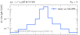
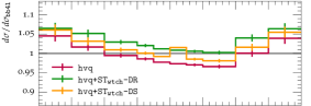
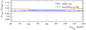
(a)

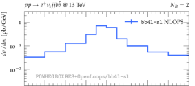
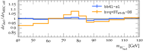
(b)

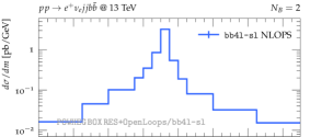
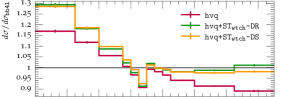
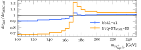
(c)

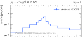
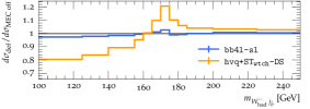
(d)

Figure 13: Distributions in the reconstructed invariant masses of the leptonically decaying $W^{+}$ (13(a)) and hadronically decaying $W^{-}$ boson (13(b)), as well as of the leptonically decaying top (13(c)) and hadronically decaying anti-top quark (13(d)). Same acceptance cuts, predictions and ratios as in Fig. 12.

Comparing bb4l-sl to hvq+${\tt ST}_{\tt wtch}$ in Figs. 13(c)–13(d), in the case of the hadronically decaying $\bar{t}$ resonance we observe a qualitatively similar behaviour as for the associated $W^{-}$ resonance: in the on-shell region hvq+${\tt ST}_{\tt wtch}$ features a deficit, while in the off-shell regions it exceeds bb4l-sl by up to 10% As discussed above for the $W^{-}$-mass distribution, these deviations can be attributed to parton-shower uncertainties, and the fact that in the $\bar{t}$-mass distribution they are much more sizeable is consistent with the fact that shower effects are much bigger than in the $W^{-}$-mass distribution (see Fig. 10(b)). Note that the same holds also for Pythia’s matrix-element corrections to hvq+${\tt ST}_{\tt wtch}$, which behave in a significantly different way on the two sides of the peak. As for the leptonic $t$ resonance, in the off-shell region below the peak the relative difference between hvq+${\tt ST}_{\tt wtch}$ and bb4l-sl turns out to be much more pronounced than in the hadronic $\bar{t}$ resonance. This is related to the fact that the leptonic resonance is much steeper due to the absence of dilution effects stemming from the hadronic $W^{-}$ decay. In particular, moving form the peak to the neighbouring bin below the peak, the cross section goes down by a factor four, while in the difference between hvq+${\tt ST}_{\tt wtch}$ and bb4l-sl we observe an abrupt change of about $-10\%$, which can be interpreted as a difference of $-2.5\%$ in the number of events that migrate from one bin to the other, as a result of QCD radiation. We also note that this abrupt change is correlated with a similarly sharp variation of Pythia’s matrix-element corrections in hvq+${\tt ST}_{\tt wtch}$. This suggests that the significant shape differences between hvq+${\tt ST}_{\tt wtch}$ and bb4l-sl may be due to parton-shower uncertainties in hvq+${\tt ST}_{\tt wtch}$ and, given the huge size of shower effects in hvq+${\tt ST}_{\tt wtch}$, the observed agreement with bb4l-sl is better than one may expect. In this respect, one should also keep in mind that on-shell generators like hvq+${\tt ST}_{\tt wtch}$are not expected to provide an accurate description of off-shell effects.

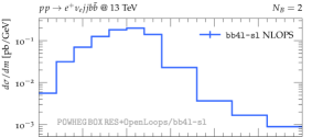
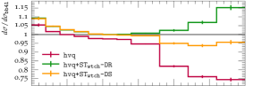
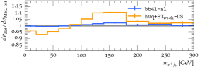
Figure 14: Distribution in the invariant mass $m_{e^{+}j_{b}}$ of the positron and the hardest $b$ jet. Same acceptance cuts, predictions and ratios as in Fig. 12.

Finally, the distribution in the invariant mass of the positron and the $b$ jet, shown in Fig. 14, features an interesting pattern of off-shell effects. In the region above the kinetic edge at $m_{e^{+}\,j_{b}}\simeq 152\,\text{GeV}$, the difference between hvq and bb4l-sl grows quite rapidly, reaching $-25\%$ at 300 GeV. At the same time, the difference between ${\tt ST}_{\tt wtch}$ predictions in DS and DR mode indicates large $t\bar{t}$–$tW$ interference effects that grow up to 20% in the tail. In spite of these large off-shell effects, at high $m_{e^{+}\,j_{b}}$ the difference between bb4l-sl and hvq+${\tt ST}_{\tt wtch}$-$\tt{DS}$ never exceeds 5%. This is quite remarkable given that shower effects are around a factor two in the tail (see Fig. 11). In the region of small $m_{e^{+}\,j_{b}}$, the DR and DS modes of hvq+${\tt ST}_{\tt wtch}$ agree, which indicates negligible $t\bar{t}$–$tW$ interference effects. Nevertheless, we observe a deviation between bb4l-sl and hvq+${\tt ST}_{\tt wtch}$, which approaches 10% in the first bin. This may be related to the very strong sensitivity of the $b$-jet mass to shower radiation in hvq+${\tt ST}_{\tt wtch}$ (see Figs. 9(d) and 12(d)).

10 Summary and conclusions

We have presented methodological improvements, new results and tools for the NLOPS description of off-shell $t\bar{t}+tW$ production with dileptonic or semileptonic decays at the LHC. In the dileptonic case, NLOPS predictions of this kind are available through the bb4l generator in Ref. Jezo:2016ujg , which is based on exact NLO matrix elements for the full $\ell^{+}\nu_{\ell}\,\ell^{\prime\,-}\bar{\nu}_{\ell^{\prime}}b\bar{b}$ production process. This provides, among others, a unified NLO description of off-shell $t\bar{t}$ and $tW$ production including their interference, as well as a NLO accurate description of all involved decay subprocesses. Within the bb4l generator, the consistent matching of off-shell matrix elements to the parton shower is guaranteed by the POWHEG–RES method, i.e. the resonance-aware extension of the POWHEG method. This technique is based on so-called resonance histories, which provide a probabilistic decomposition of the full off-shell process into separate production and decay subprocesses. Such resonance histories play a key role in order to guarantees the correct NLO shapes of resonances. Moreover, they make it possible to associate NLO radiation to specific subprocesses and to generate one POWHEG emissions from each subprocess, i.e. multiple POWHEG emissions per event.

In this paper we have presented a new version of the dileptonic bb4l generator together with a new generator that provides the same kind of NLOPS accuracy for the case of off-shell $t\bar{t}+tW$ production with semileptonic decays. These new dileptonic and semileptonic generators are both implemented in the bb4l framework and are called bb4l-dl and bb4l-sl, respectively. Technically, semileptonic Les Houches events can be generated in an efficient way by re-processing pre-existing dileptonic events.

The definition of the physics content of the bb4l-sl generator involves nontrivial subtleties, which are due to the presence of various irreducible backrounds that contribute to the same signature and interfere with $t\bar{t}+tW$ production. Based on a detailed analysis of such irreducible backgrounds, we have implemented a theoretical process definition, which guaratees that bb4l-sl includes all possible $t\bar{t}+tW$ contributions and the $t\bar{t}$–$tW$ interference, while all relevant backgrounds—such as $t$- and $s$-channel single-top production processes with extra jet radiation—can be separated and simluated with independent tools. In practice, we have adopted a process definition based on the same LO and NLO Feynman diagrams that contribute to the dileptonic process, plus additional QCD correction effects associated with the hadronic $W\to q\bar{q}^{\prime}$ decay at NLO. For the latter we have adopted a double-pole approximation that retains all Feynman diagrams with subtopologies of type $pp\to W^{+}W^{-}b\bar{b}$ plus extra radiation.

In addition to the new bb4l-sl generator, we have presented two significant methodological improvements that are implemented both within bb4l-dl and bb4l-sl.

The first improvement deals with spurious effects of $\mathcal{O}(\alpha_{\rm S}^{2})$ that arise from the inconsistent perturbative treatment of decay widths at NLO. In the context of the NWA, this problem is well known and can be solved by means of a systematic perturbative expansion of terms of the form $1/\Gamma_{\mathrm{NLO}}$. Off-shell NLO calculations, whose zero-width limit coincides with the NWA, suffer from the same problem. However, a direct expansion of $1/\Gamma_{\mathrm{NLO}}$ terms is not possible in the off-shell case, since such terms are not explicitly present. Nevertheless, as we have shown, the inverse-width expansion can be generalised to NLO calculations for arbitrary off-shell processes and their matching to parton showers in the POWHEG–RES framework. As we pointed out, in the case of off-shell $t\bar{t}+tW$ production this inverse-width expansion plays an important role for the consistent normalisation of total and differential NLO cross section. In fact, if left uncancelled, spurious terms can shift the cross section by up to $7\%$, which exceeds the size of the overall off-shell and $tW$ contributions, and is similarly large as the complete NLO corrections to top decays.

The second methodological improvement concerns the definition of the POWHEG–RES resonance histories for off-shell $t\bar{t}+tW$ production and decays. While the original bb4l generator was effectively restricted to resonance histories of $t\bar{t}$ type, the new bb4l-sl and bb4l-sl generators implement also new histories of $tW$ type. In addition, for both types of resonance histories we have implemented realistic history probabilities based on Born matrix elements. This guarantees a reliable separation of events that are dominated by $t\bar{t}$ or $tW$ production, and a more consistent treatment of the hardest QCD radiation for these different types of events. In the case of bb4l-dl, this improved POWHEG–RES implementation was compared to the one of Ref. Jezo:2016ujg for several distributions, finding only minor numerical differences. This suggests that bb4l predictions are largely free from uncertainties related to technical choices in the definition of resonance histories.

In another technical study we have compared predictions of the bb4l-sl and bb4l-dl generators in a way that highlights those differences that originate from QCD effects associated with the hadronic $W$ decay in bb4l-sl. In particular, we have isolated QCD effects stemming from jet fragmentation and jet contamination, and we have analysed their impact on various differential observables.

Finally, we have presented a tuned comparison of bb4l-sl against the on-shell POWHEG generators of $t\bar{t}$ and $tW$ production, i.e. hvq and ${\tt ST}_{\tt wtch}$. In this context, in spite of the deficits of the on-shell generators in terms of physical content and perturbative accuracy, for several observables we have observed an unexpected level of agreement. As we have demonstrated, this good agreement is due also to Pythia’s built-in matrix-element corrections, which promote the formal accuracy for top and $W$ decays within on-shell generators from LO to approximate NLO. The most significant deviations between on-shell and off-shell generators arise, among others, from the $t\bar{t}$–$tW$ interference, which is described with NLO accuracy within bb4l, while in the on-shell case it can only be estimated at LO by comparing different version of the ${\tt ST}_{\tt wtch}$ generator.

The presented results deal only with selected kinematic distributions that are typically studied in the context of $t\bar{t}$ production, while we did not investigate more exclusive phase-space regions where off-shell and $tW$ contributions can be strongly enhanced. In that case, and in general, bb4l-dl and bb4l-sl are expected to provide more reliable predictions as compared to the on-shell NLOPS generators.

The methodology developed in this paper is also applicable to off-shell $t\bar{t}+tW$ production with fully hadronic decays, and will make it possible to generate fully inclusive event samples including dileptonic, semileptonic, and hadronic decays.

Appendix A Real-to-Born kinematic mappings

In this appendix we provide the explicit form of the kinematic mappings that enter the new matrix-element–based resonance histories presented in Sect. 4.2. The definition of such histories is based on the weights (4.2), and their alternative versions (4.2)–(4.2). Such weights are defined in the Born phase space and are extended to the real-emission phase space through real-to-Born kinematic mappings as specified in (66)–(67). The goal of these real-to-Born mappings, which transform real-emission events into Born events,

$$\phi_{\mathrm{R}}\to\widetilde{\Phi}_{\mathrm{B},c}\,,$$ (96)

is to ensure that the accuracy of the $t\bar{t}$ and $tW$ Born probabilities, which is guaranteed by the usage of Born matrix elements, is not spoiled by their extension to the real-emission phase space. To this end, as discussed in Sect. 4.2, the mappings (96) are designed such as to preserve the key quantities that control the relative probabilities of $t\bar{t}$ and $tW$ histories, namely the virtualities of the $W^{+}b$ and $W^{-}\bar{b}$ systems, as well as the transverse energies of the $b$ or $\bar{b}$ quarks that are potentially involved into initial-state $g\to b\bar{b}$ splittings in the case of $tW$ production.

The real-to-Born mappings (96) are independent of the resonance history and depend only on the collinear sector $c$. More precisely, they only depend on whether the emitter is an initial-state (IS) particle or a final-state (FS) $b$ or $\bar{b}$ quark. These different cases are discussed in App. A.1 and A.2.

A.1 The FS case

In the case of final-state radiation there are only two possible collinear sectors, which correspond to $b\to bg$ or $\bar{b}\to\bar{b}g$ splittings and can be associated, respectively, to an off-shell $t\to\ell^{+}\nu_{l}bg$ or $\bar{t}\to\ell^{-}\bar{\nu}_{l}\bar{b}g$ decay. In the following we refer to this decay as the radiative top decay, for which we use the charge-independent notation

$$t\to\ell\nu bg\,.$$ (97)

In the FS case, the real-to-Born mapping (96) acts only on the subset of momenta that arise from the radiative top decay, which is identified according to the actual collinear sector. Such momenta are labelled as

$$\{p^{\prime}_{l},p^{\prime}_{\nu},p^{\prime}_{b},p_{g}^{\prime}\}\,\subset\,\Phi_{\mathrm{R}}\,,$$ (98)

while for the related momenta of the $bg$ system, the off-shell $W$ boson and the off-shell top quark, we use the symbols

$$p^{\prime}_{W}\,=\,p^{\prime}_{l}+p^{\prime}_{\nu}\,,\qquad p^{\prime}_{bg}\,=\,p^{\prime}_{b}+p^{\prime}_{g}\,,\qquad p^{\prime}_{t}\,=\,p^{\prime}_{W}+p^{\prime}_{bg}\,.$$ (99)

The real-to-Born FS mapping turns the real-emission momenta (98)–(99) into the Born momenta

$$\{p_{l},p_{\nu},p_{b}\}\,\subset\,\widetilde{\Phi}_{\mathrm{B},c}\,,$$ (100)

and

$$p_{W}\,=\,p_{l}+p_{\nu}\,,\qquad p_{t}\,=\,p_{W}+p_{b}\,.$$ (101)

All external momenta that do not belong to the radiative top system are kept unchanged. Thus, also the off-shell momentum of the radiating top itself remains unchanged, i.e.

$$p_{t}\,=\,p^{\prime}_{t}\,.$$ (102)

Within the radiating-top system, the real-to-Born mapping can be defined as a transformation

$$p_{bg}^{\prime}\to p_{b}\,,$$ (103)

which turns the off-shell real momenum of the $bg$ system into an on-shell $b$-quark Born momentum. The three d.o.f. of $\vec{p}_{b}$ can be parametrised by its components in the beam direction, $p_{\parallel,b}$, its magnitude in the transverse plane, $|\vec{p}_{\perp,b}|$, and its angle $\phi_{bt}$ w.r.t. the parent top momentum in the transverse plane, which obeys

$$\cos\phi_{bt}\,=\,\frac{{\vec{p}}_{\perp,b}\cdot{\vec{p}}^{\,\prime}_{\perp,t}}{|{\vec{p}}_{\perp,b}|\,|{\vec{p}}^{\,\prime}_{\perp,t}|}\,.$$ (104)

Once $\vec{p}_{b}$ is fixed, the $b$-quark energy is given by $E_{b}=\sqrt{|\vec{p}_{b}|^{2}+m_{b}^{2}}$, and for the $W$-boson momentum in the Born phase space we have

$$p_{W}\,=\,p_{t}-p_{b}\,=\,p^{\prime}_{t}-p_{b}\,.$$ (105)

As discussed in the following, the three d.o.f. of $\vec{p}_{b}$ are fixed in a way that preserves the $W$-boson virtuality, and, if possible, also the transverse energy of the $bg$ system and its direction. For the $W$ virtuality we always impose

$$p_{W}^{2}\,=\,p_{W}^{\prime 2}\,,$$ (106)

by using

$$p_{W}^{2}\,=\,(p_{t}-p_{b})^{2}\,=\,p_{t}^{2}+p_{b}^{2}-2p_{t}\cdot p_{b}\,=\,p^{\prime 2}_{t}+m_{b}^{2}-2p^{\prime}_{t}\cdot p_{b}\,.$$ (107)

In terms of $|p_{\perp,b}|$, $p_{\parallel,b}$, and $\cos\phi_{bt}$, this yields

$$p_{t}^{\prime 2}+m_{b}^{2}-2\left[E^{\prime}_{t}\sqrt{p^{2}_{\parallel,b}+|\vec{p}_{\perp,b}|^{2}+m_{b}^{2}}-|{\vec{p}}^{\,\prime}_{\perp,t}||\vec{p}_{\perp,b}|\cos\phi_{bt}-p^{\prime}_{\parallel,t}\,p_{\parallel,b}\right] = p_{W}^{\prime 2}\,,$$ (108)

which corresponds to a quadratic equation in $p_{\parallel,b}$, with solutions

$$p_{\parallel,b}\,=\,\frac{p^{\prime}_{\parallel,t}\,a\pm E^{\prime}_{t}\sqrt{\Delta}}{c}\,,$$ (109)

where $E^{\prime}_{t}=\sqrt{|{\vec{p}}^{\,\prime}_{t}|^{2}+m_{t}^{2}}$,

$$a = p_{t}^{\prime 2}+m_{b}^{2}-p_{W}^{\prime 2}+2|{\vec{p}}^{\,\prime}_{\perp,t}||\vec{p}_{\perp,b}|\cos\phi_{bt}\,,\qquad c\,=\,2E^{2}_{t}-p^{2}_{\parallel,t}\,,$$ (110)

and

$$\Delta = a^{2}-2\,(|\vec{p}_{\perp,b}|^{2}+m_{b}^{2})\,c\,.$$ (111)

Between the two solutions in (109) we always pick the one where $p_{\parallel,b}$ is closer to $p^{\prime}_{\parallel,bg}$.

Before fixing $p_{\parallel,b}$ according to (109), i.e. in a way that preserves the $W$-boson virtuality, when possible we fix the values of $|\vec{p}_{\perp,b}|$ and $\cos\phi_{bt}$ in a way that preserves the transverse energy and the direction of the $b$ quark. This is not always possible, since in some cases the latter two conditions lead to a negative determinant, $\Delta<0$, in (109). For this reason we set $|\vec{p}_{\perp,b}|$ and $\cos\phi_{bt}$ according to different criteria in the following three cases.

• By default we choose $|\vec{p}_{\perp,b}|$ in such a way that the resulting $b$-quark transverse energy, $E_{\perp,b}=\sqrt{|{\vec{p}}_{\perp,b}|^{2}+m_{b}^{2}}$, is equal to the one of the original bg system, i.e.

  $$E_{\perp,b}\,=\,E^{\prime}_{\perp,bg}\,=\,\sqrt{|{\vec{p}}^{\,\prime}_{\perp,bg}|^{2}+(p^{\prime}_{bg})^{2}}\,.$$ (112)

  Moreover, we also align the direction of the $b$ quark to the one of the original $bg$ system by imposing

  $$\cos\phi_{bt}\,=\,\cos\phi_{bt}^{\prime}\,=\,\frac{{\vec{p}}^{\,\prime}_{\perp,bg}\cdot{\vec{p}}^{\,\prime}_{\perp,t}}{|{\vec{p}}^{\,\prime}_{\perp,bg}|\,|{\vec{p}}^{\,\prime}_{\perp,t}|}\,.$$ (113)

  These choices are applied to all events for which they yield $\Delta>0$. Otherwise we switch to case (ii) or (iii).

• If $\Delta<0$ in case (i), then we try to impose only (112) and to fix $\cos\phi_{bt}$ in such a way that $\Delta=0$, which corresponds to a linear equation in $\cos\phi_{bt}$. These choices are applied to all events for which they yield a physical direction, i.e. $|\cos\phi_{bt}|\leq 1$. Otherwise we switch to case (iii).

• If $\Delta=0$ yields unphysical solutions with $|\cos\phi_{bt}|>1$ in case (ii), then we set $\cos\phi_{bt}=\pm 1$, picking the same sign as the one of the unphysical solution, and we set $|\vec{p}_{\perp,b}|$ such that $\Delta=0$, which is always possible.

Once the $b$-quark momentum is fixed as described above, the $W$-momentum is determined as indicated in (105). Finally, the momenta $\{p_{\ell},p_{\nu}\}$ of the $W$-decay products, are obtained from the related momenta $\{p^{\prime}_{\ell},p^{\prime}_{\nu}\}$ by applying a sequence of two boosts that transform $p^{\prime}_{W}$ to its rest frame and subsequently turn it into $p_{W}$.

Note that in the strict soft limit the result of this mapping coincides with the underlying Born event.

A.2 The IS case

In the IS case we have implemented real-to-Born mappings that preserve the virtuality of all relevant $W$ bosons and $Wb$ pairs together with the invariant mass of the virtual $b$ quark that is involved in the initial-state $g\to b\bar{b}$ splitting in the case of $pp\to tWb$ production. To this end, as detailed below, we have determined the most likely parton-level topology of type

$$IJ\rightarrow tWb+X\,,$$ (114)

where $I$ and $J$ are the initial-state partons, $X$ is the parton emitted via ISR, $t$ denotes a generic (off-shell) top or anti-top quark that undergoes a three-body decay, and $Wb$ is the off-shell $W^{+}b$ or $W^{-}\bar{b}$ system with the highest probability of being the non-resonant $Wb$ system resulting from $tWb$ production. In the following, the bottom quark or anti-quark $b$ that belongs to the “non-resonant” $Wb$ system is referred to as the $b$ spectator, since it corresponds to the $b$ (anti-)quark with the highest probability of stemming from the initial-state $g\to b\bar{b}$ splitting within a $Wtb$ production subprocess.

The general form of our real-to-Born mappings is

$$p^{\prime}_{I},\,p^{\prime}_{J},\,p^{\prime}_{t},\,p^{\prime}_{X}\,\;\rightarrow\;p_{I},\,p_{J},\,p_{t}\,,$$ (115)

i.e. the momenta of the non-resonant $Wb$ system are kept unchanged. In order to determine the most likely topology of type (114) we consider eight different cases—and corresponding probabilities—that arise from all possible combinations of the following options.

• The initial-state leg that emits ISR is $E=I$ or $E=J$. The corresponding probability is chosen as

  $$P^{(\mathrm{em})}_{E}\,=\,\frac{1}{(1-\cos\phi_{E})^{2}}\qquad\mbox{with}\qquad\cos\phi_{E}\,=\,\frac{{\vec{p}}^{\,\prime}_{E}\cdot{\vec{p}}^{\,\prime}_{X}}{|{\vec{p}}^{\,\prime}_{E}||{\vec{p}}^{\,\prime}_{X}|}\,.$$ (116)

• The initial-state leg that undergoes a $g\to b\bar{b}$ splitting is $S=I$ or $S=J$. The corresponding probability is chosen as

  $$P^{(g\to b\bar{b})}_{S}\,=\,\frac{1}{{q}^{\prime 2}_{S}-m_{b}^{2}}\,,$$ (117)

  where $q_{S}$ is the momentum of the virtual $b$ quark that results from the $g\to b\bar{b}$ splitting, i.e.

  $${q}^{\prime}_{S}\,=\,\begin{cases}p^{\prime}_{S}-p^{\prime}_{b}&\;\mbox{for}\;S\neq E\,,\\ p^{\prime}_{S}-p^{\prime}_{b}-p^{\prime}_{X}&\;\mbox{for}\;S=E\,.\\ \end{cases}$$ (118)

• The non-resonant $Wb$ system corresponds either to the $W^{+}b$ or to the $W^{-}\bar{b}$ system. In order to discriminate between these two options we make use of the probability

  $$P^{(\mathrm{top})}_{Wb}\,=\,\frac{m_{t}^{2}}{\left[(p^{\prime}_{W}+p^{\prime}_{b})^{2}-m_{t}^{2}\right]^{2}+\Gamma_{t}^{2}m_{t}^{2}}\,.$$ (119)

The most likely topology (115) is selected as the one that maximises the combined “probability”

$$P\,=\,\frac{P^{(\mathrm{em})}_{E}\,P^{(g\to b\bar{b})}_{S}}{P^{(\mathrm{top})}_{Wb}}.$$ (120)

Before we proceed with the definition of our kinematic mapping let us introduce the auxiliary off-shell momentum

$${k}^{\prime}_{E}\, = \,p^{\prime}_{E}-p^{\prime}_{X}\,,$$ (121)

where $p^{\prime}_{E}$ is the momentum of the initial-state leg that radiates, and the auxiliary on-shell momentum

$${\tilde{p}}_{E}=xp^{\prime}_{!E}+{k}^{\prime}_{E}\qquad\text{ with }\qquad x=-\frac{{k}^{\prime 2}_{E}}{(p^{\prime}_{!E}+{k}^{\prime}_{E})^{2}-{k}^{\prime 2}_{E}}\,,$$ (122)

where $!E$ corresponds to the initial-state leg that does not radiate, i.e. $!E=J(I)$ for $E=I(J)$. By construction ${\tilde{p}}^{2}_{E}=0$. For the definition of the real-to-Born mappings we consider the following two cases.

• If the ISR emitter and the leg that undergoes the $g\to b\bar{b}$ splitting are different, i.e. $E\neq S$, than the form (115) of the mapping automatically guarantees that all external particles that are connected to the $g\to b\bar{b}$ splitting are kept unchanged. In this case, $p^{\prime}_{E}$ and $p^{\prime}_{t}$ are turned into the Born momenta

  $$p_{E} = y_{A}{\tilde{p}}_{E}\,,\qquad p_{t}\,=\,p^{\prime}_{t}+y_{A}{\tilde{p}}_{E}-{k}^{\prime}_{E}\,,$$ (123)

  where

  $$y_{A}=-\frac{{k}^{\prime}_{E}\cdot{k}^{\prime}_{E}-2p^{\prime}_{t}\cdot{k}^{\prime}_{E}}{2\left(p^{\prime}_{t}\cdot{\tilde{p}}_{E}-{k}^{\prime}_{E}\cdot{\tilde{p}}_{E}\right)}$$ (124)

  guarantees that the virtuality of the resonant top quark is preserved, i.e. $p^{2}_{t}=p^{\prime 2}_{t}$.

• If the ISR emitter is instead the same leg that undergoes the $g\to b\bar{b}$ splitting, i.e. $E=S$, we again manipulate the initial-state leg $E$ and the momentum of the resonant top quark, which are turned into

  $$p_{E} = y_{B}{\tilde{p}}_{E}\,,\qquad p_{t}\,=\,p^{\prime}_{t}+(y_{B}-1){k}^{\prime}_{E}-zp^{\prime}_{!E}\,.$$ (125)

  Here, in order to preserve the invariant mass of the virtual $b$ quark in the $g\to b\bar{b}$ splitting, i.e. $q^{2}_{S}=(p_{S}-p_{b})^{2}={q}^{\prime 2}_{S}$, and the virtuality of the resonant top quark, i.e. $p^{2}_{t}=p^{\prime 2}_{t}$, we choose

  $$y_{B} = -\frac{{k}^{\prime 2}_{E}-2p^{\prime}_{!b}\cdot{k}^{\prime}_{E}}{2p^{\prime}_{!b}\cdot{k}^{\prime}_{E}}\ ,\qquad z\,=\,\frac{(y_{B}-1){k}^{\prime}_{E}\cdot\left(2p^{\prime}_{t}+(y_{B}-1){k}^{\prime}_{E}\right)}{2p^{\prime}_{!E}\cdot\left(p^{\prime}_{t}+(y_{B}-1){k}^{\prime}_{E}\right)}\ ,$$ (126)

  where $p_{!b}$ is the momentum of the $b$ quark stemming form the decay of the resonant top quark.

Finally, in both cases we boost the decay products of the resonant top quark according to the $p^{\prime}_{t}\to p_{t}$ transformation.

In the soft limit this mapping reproduces the underlying Born kinematics with the soft radiation removed, and in the collinear limit it reproduces it with the momentum of the collinear radiation subtracted from the momentum of the emitter.

Appendix B The bb4l-sl definition of semileptonic $t\bar{t}+tW$ production and decay

As discussed in Sect. 5, the physics content of the bb4l-sl generator corresponds to the ingredients of the full process (70) that satisfy the selection criteria S1–S3 (see Sect. 5.1). This selection captures all possible contributions associated with off-shell $t\bar{t}+tW$ production and decays to semileptonic final states. Moreover, it is in one-to-one correspondence with the ingredients of the dileptonic bb4l-dl generator, with the addition of QCD effects in $W\to q\bar{q}$ decays. In the following, we present technical studies that justify this process definition at LO and NLO. In doing so, we focus on the contributions that satisfy S1, i.e. the contributions of order $\alpha_{\rm S}^{2}\alpha^{4}$ and $\alpha_{\rm S}^{3}\alpha^{4}$, and we analyse the effect of the selection steps S2 and S3.

The studies presented in this appendix were done with Sherpa Sherpa:2019gpd for the case of $\ell^{-}\bar{\nu}_{\ell}jjb\bar{b}$ production, while the charge-conjugated process yields qualitative identical results. All predictions were obtained with the setup of Sect. 6, and requiring two light jets plus either one or more than one $B$ jet with $R=0.5$, $p_{\rm T}>25\,$GeV and $|\eta|<2.5$, as well as a charged lepton with $p_{\rm T}>25\,$GeV and $|\eta|<2.5$, and no cuts on the neutrino.

B.1 Effect of the S2 and S3 selections at LO

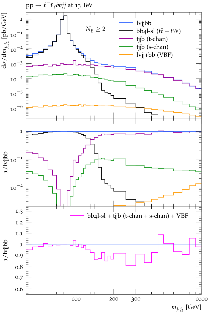
(a)

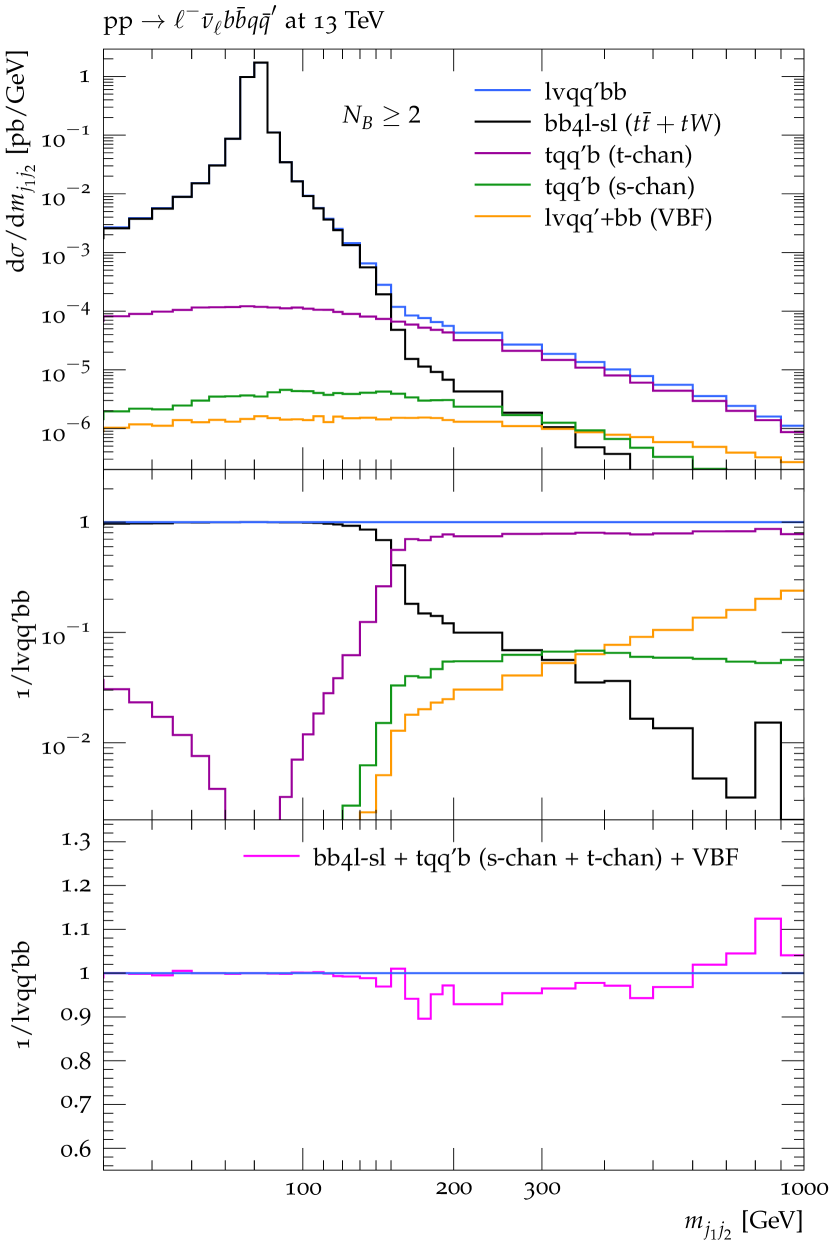
(b)

Figure 15: Contributions of $\mathcal{O}(\alpha_{\rm S}^{2}\alpha^{4})$ to the distribution in the invariant mass of the two light jets for off-shell $\ell^{-}\bar{\nu}_{\ell}jjb\bar{b}$ (15(a)) and $\ell^{-}\bar{\nu}_{\ell}q\bar{q}^{\prime}b\bar{b}$ (15(b)) production in the phase space with $N_{B}\geq 2$ $B$ jets. In both cases, exact off-shell predictions are compared to the individual contributions from $t\bar{t}+tW$ production (corresponding to bb4l-sl at LO), $t$- and $s$-channel single-top production, and $Wjj+b\bar{b}$ production via VBF. The mid panel shows ratios of individual contributions wrt the full off-shell process at hand, while the lower panel shows the same ratio for the additive combination of the $t\bar{t}+tW$ plus single-top plus VBF production subprocesses.

In Fig. 15 we present the distribution in the invariant mass of the two light jets in the phase space with two or more $B$-jets. The plotted $m_{j_{1}j_{2}}$ range includes a wide region around the $W\to jj$ resonance and extends up to dijet masses of 1 TeV.

The predictions in Fig. 1515(a) correspond to the outcome of the S1 selection, i.e. the off-shell $\ell^{-}\bar{\nu}_{\ell}jjb\bar{b}$ production process at $\mathcal{O}(\alpha_{\rm S}^{2}\alpha^{4})$, while in Fig. 1515(b) we show the outcome of the S1+S2 selection steps, which corresponds to off-shell $\ell^{-}\bar{\nu}_{\ell}q\bar{q}^{\prime}b\bar{b}$ production at $\mathcal{O}(\alpha_{\rm S}^{2}\alpha^{4})$ with a $q\bar{q}^{\prime}$-pair consistent with a $W^{+}$ decay, i.e. $u\bar{d}$ or $c\bar{s}$. In Figs. 1515(a)–15(b) we also show the contributions of the most significant subprocesses, namely off-shell $t\bar{t}+tW$ production, $s$- and $t$-channel single-top production, and $Wjj$ production via VBF in association with a $b\bar{b}$ pair (see Tab. 3 and the discussion in Sect. 5.1). Here the $t\bar{t}+tW$ contribution should be understood as the physics content of bb4l-sl at LO, and is equivalent to the outcome of the S1+S2+S3 selection steps. This contribution is the same in Fig. 1515(a) and 1515(b), while in Fig. 1515(b) the single-top and VBF contributions have a smaller cross section due to the requirement of a $q\bar{q}^{\prime}$ pair in the final state.

The absolute predictions in the upper panels of Figs. 1515(a)–15(b) demonstrate that the total cross section is strongly dominated by the $W\to jj$ resonance and is very well approximated by off-shell $t\bar{t}+tW$ production and decay, i.e. bb4l-sl, which is the only subprocess with a $W\to jj$ resonance. When a $q\bar{q}^{\prime}$ pair is required (Fig. 1515(b)) the bb4l-sl contribution provides an almost perfect approximation in a broad region around the resonance, with sub-percent precision for $|m_{j_{1}j_{2}}-m_{W}|<30\,$GeV.

Extra contributions become significant only for $m_{j_{1}j_{2}}\gtrsim 130\,$GeV and can exceed bb4l-sl by more than two orders of magnitude in the off-shell tail. In this highly off-shell regime the $pp\to\ell^{-}\bar{\nu}_{\ell}q\bar{q}^{\prime}b\bar{b}$ process is dominated by $t$-channel single-top production, and receives sizeable contributions also from $s$-channel single-top production and, at very large dijet masses, also from the VBF subprocess. As demonstrated in the lower panel of Fig. 1515(b), the incoherent sum of the bb4l-sl plus the single-top and the VBF subprocesses agrees with the exact description based on off-shell $\ell^{-}\bar{\nu}_{\ell}q\bar{q}^{\prime}b\bar{b}$ matrix elements at the sub-percent level for $m_{j_{1}j_{2}}<150\,$GeV, and at the level of $5\%$ in the entire plotted range above 150 GeV. Extending this analysis of the $m_{j_{1}j_{2}}$ distribution to the phase space with $N_{B}=1$ $B$-jets (not show here) we found a qualitatively and quantitatively similar behaviour as in the $N_{B}\geq 2$ phase space.

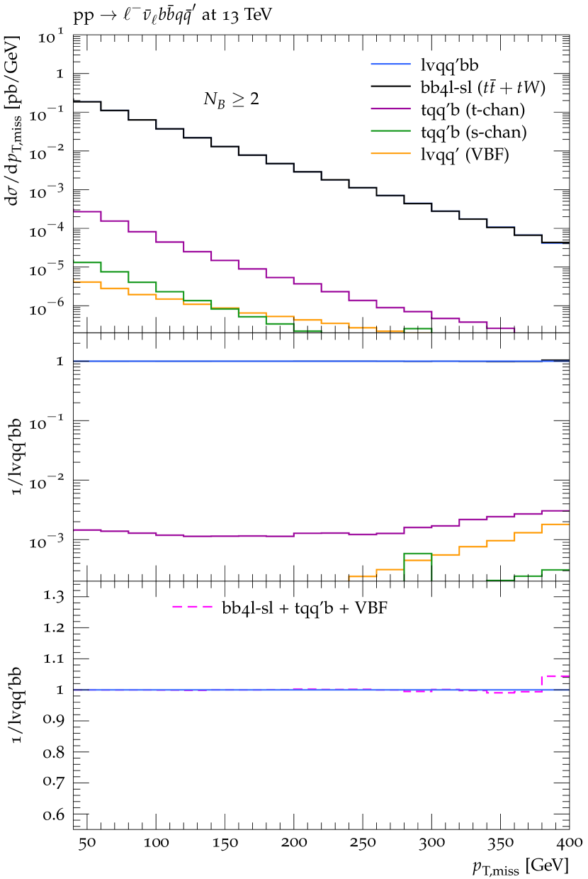
(a)

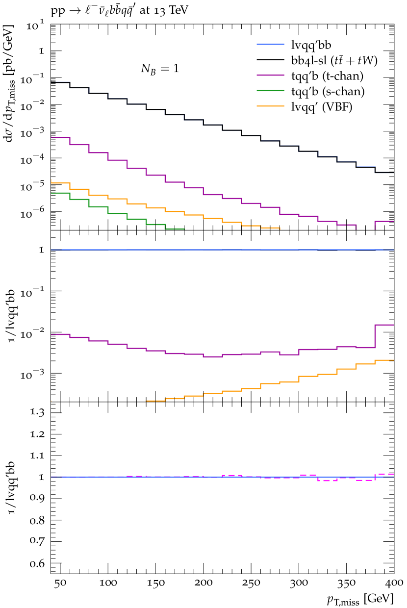
(b)

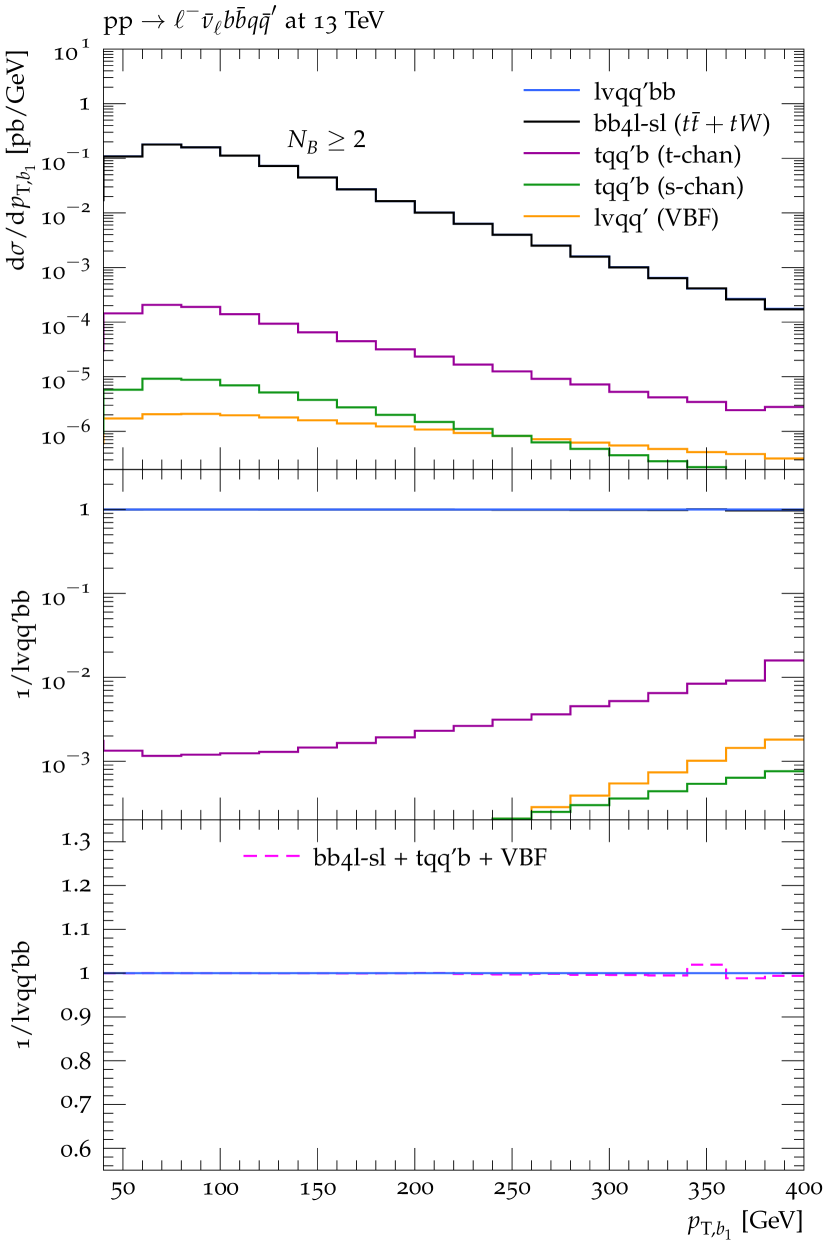
(c)

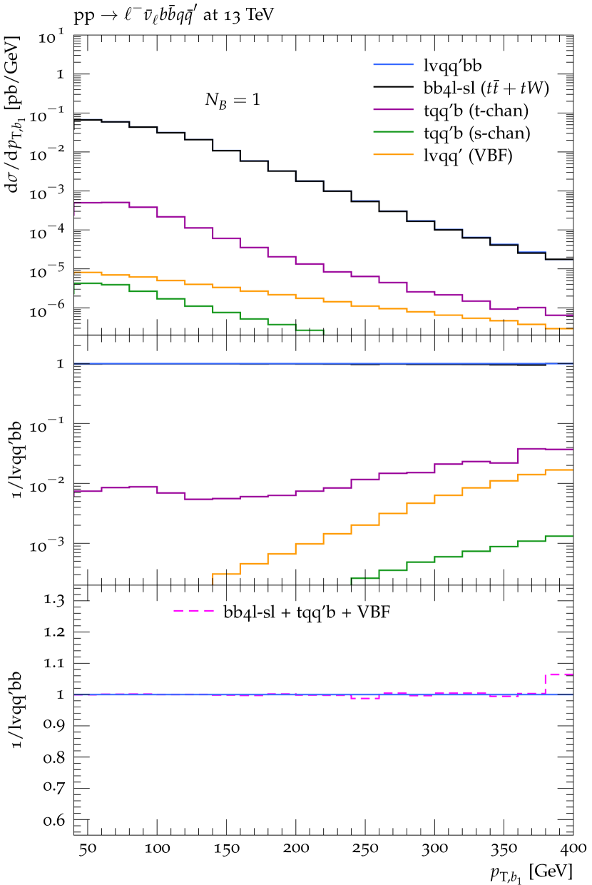
(d)

Figure 16: Off-shell $\ell^{-}\bar{\nu}_{\ell}q\bar{q}^{\prime}b\bar{b}$ production at $\mathcal{O}(\alpha_{\rm S}^{2}\alpha^{4})$ in the phase space with $N_{B}\geq 2$ (left) and $N_{B}=1$ (right) $B$-jets: distributions in the missing $p_{\mathrm{T}}$ (16(a)–16(b)) and in the $p_{\mathrm{T}}$ of the leading $B$-jet (16(c)–16(d)). Same predictions and ratios as in Fig. 1515(b).

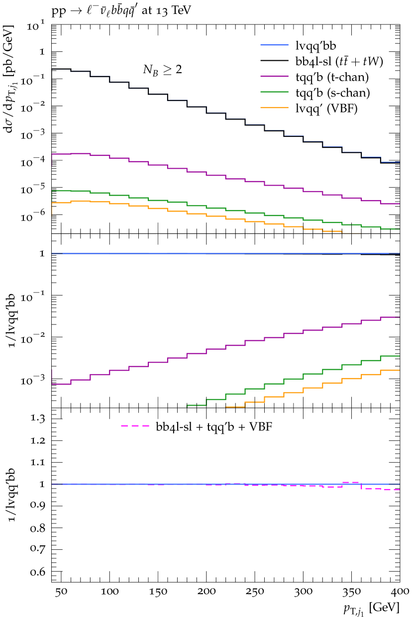
(a)

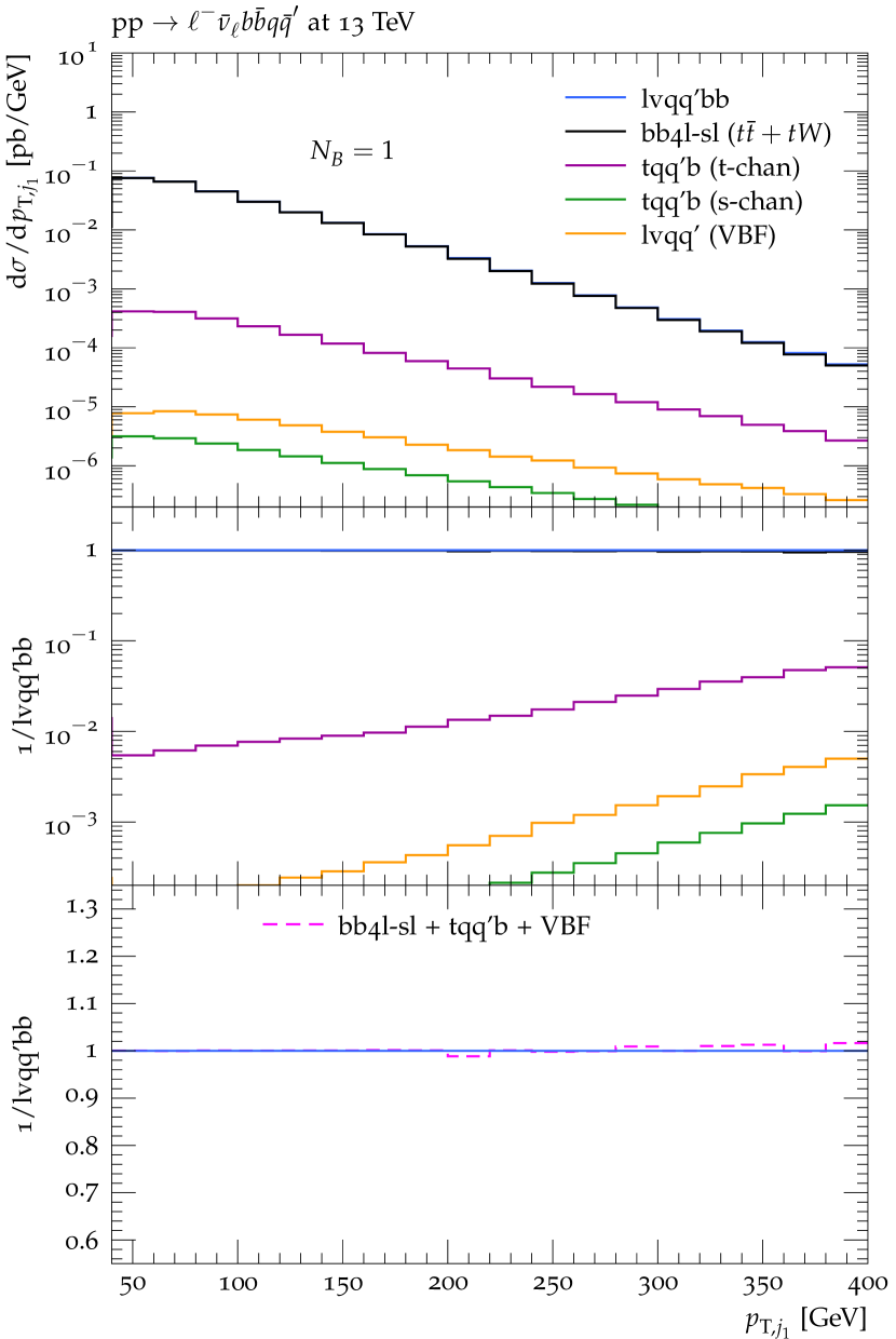
(b)

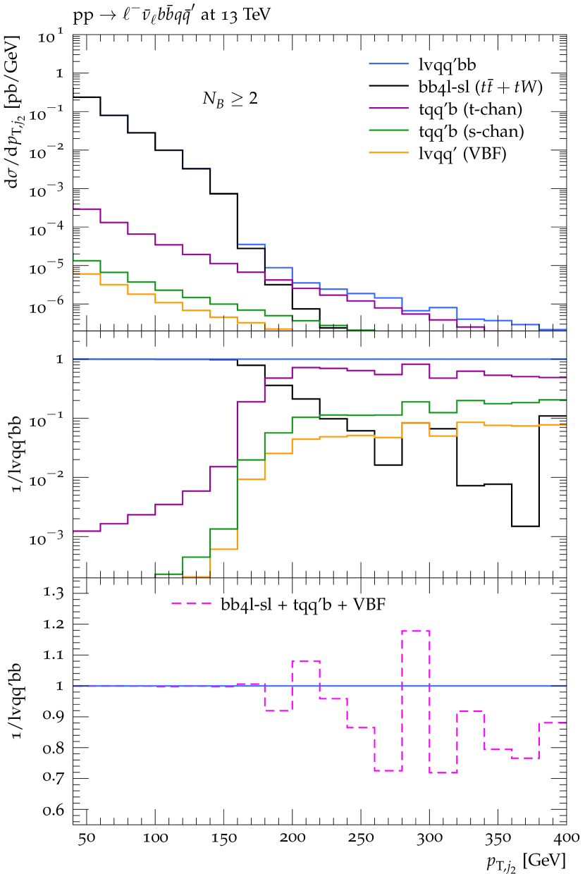
(c)

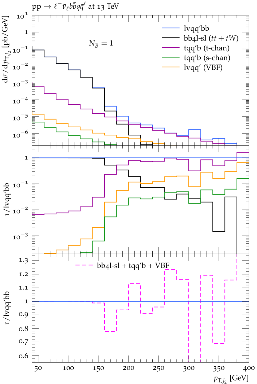
(d)

Figure 17: Off-shell $\ell^{-}\bar{\nu}_{\ell}q\bar{q}^{\prime}b\bar{b}$ production at $\mathcal{O}(\alpha_{\rm S}^{2}\alpha^{4})$: distributions in the $p_{\mathrm{T}}$ of the first (17(a)–17(b)) and of the second (17(c)–17(d)) light jet. Same predictions and ratios as in Fig. 16.

Focussing on the $\ell\nu_{l}q\bar{q}^{\prime}b\bar{b}$ signature, in Figs. 16–17 the above comparisons are extended to four different transverse-momentum distribution in the phase-space regions with two light jets plus $N_{B}\geq 2$ or $N_{B}=1$ $B$-jets.

For the distributions in the missing $p_{\mathrm{T}}$ (Fig. 1616(a)–16(b)), in the $p_{\mathrm{T}}$ of the leading $B$-jet (Fig. 1616(c)–16(d)), and in the $p_{\mathrm{T}}$ of the leading light jet (Fig. 1717(a)–17(b)), the relative weights of the various subprocesses vary more smoothly as compared to the case of the $m_{j_{1}j_{2}}$ distribution. At moderate transverse momenta, the hierarchy of the different contributions is similar as in the $W$-resonance region of Fig. 15, while in the high-$p_{\mathrm{T}}$ tails the relative importance of the single-top and VBF subprocesses can increase, depending on the observable. For these three $p_{\mathrm{T}}$ distributions we observe a fairly similar behaviour in the $N_{B}\geq 2$ and $N_{B}=1$ regions, and we find that the bb4l-sl contribution agrees with the full $\ell^{-}\bar{\nu}_{\ell}q\bar{q}^{\prime}b\bar{b}$ prediction at the level of one percent or better, with the only exception of the tail of the leading-jet $p_{\mathrm{T}}$ distribution, where above 250 GeV the weight of the $t$-channel single-top subprocess can amount to several percent.

The distribution in the $p_{\mathrm{T}}$ of the second light jet, shown in Fig. 1717(c)–17(d), reveals a somewhat different picture. In the region with $p_{\mathrm{T},j_{2}}<150\,$GeV, which contains the bulk of the cross section, the bb4l-sl contribution still agrees with the fully off-shell description at the sub-percent level. However, at $p_{\mathrm{T},j_{2}}\simeq 150\,$GeV the single-top and VBF contributions become rapidly more important, and at $p_{\mathrm{T},j_{2}}>200\,$GeV they dominate the entire cross section. We observe that this transition is due to the abrupt suppression of $t\bar{t}+tW$ production, which goes down by one to two orders of magnitude within two bins. For this reason, the region above 200 GeV suffers from limited Monte Carlo statistics.

We investigated a large number of further kinematic distributions and we observed a consistent picture throughout: whenever single-top and VBF processes are suppressed with respect to $t\bar{t}+tW$ production, the bb4l-sl contribution agrees with the complete off-shell calculation at or below the percent level. Moreover generally, the incoherent superposition of $t\bar{t}+tW$ production with the single-top and VBF subprocesses provides an excellent approximation in the full phase space.

These observations justify the treatment of off-shell $t\bar{t}+tW$ production with semileptonic decays, as defined in bb4l-sl, as a separate process, i.e. neglecting interferences with the other ingredients of $pp\to\ell^{-}\bar{\nu}_{\ell}q\bar{q}^{\prime}b\bar{b}$.

B.2 Effect of the S3 selection at NLO

In the order to investigate the consistency of the bb4l-sl process definition beyond LO, we have extended the studies of Sect. B.1 to the real-emission process

$$pp\to\ell^{-}\bar{\nu}_{\ell}q\bar{q}^{\prime}b\bar{b}j\,.$$ (127)

In order to avoid IR divergences, for the additional light jet we require $p_{{\rm T},j}>p_{{\rm T},{\rm min}}$, and to minimise the bias due to this technical cut we compare three different variants with $p_{{\rm T},{\rm min}}=20\,\text{GeV},5\,\text{GeV},$ and 1 GeV.

The above process corresponds to the real-emission contribution to the outcome of the S1+S2 selection steps, and in the following we investigate the effect of the additional S3 selection, which isolates the $t\bar{t}+tW$ contribution as define in bb4l-sl. In Figs. 18–20 we present the same set of distributions as in Sect. B.1 in the $N_{B}\geq 2$ and $N_{B}=1$ regions. Exact off-shell predictions for the process (127) are compared to the contributions of the most relevant subprocesses, which are the same as in Sect. B.1 with the exception of the VBF subprocess, which turns out to be completely negligible and is thus omitted. In the case of the $t\bar{t}+tW$ subprocess, i.e. bb4l-sl, we also show the effect of disabling QCD radiation in $W\to q\bar{q}^{\prime}$ decays.

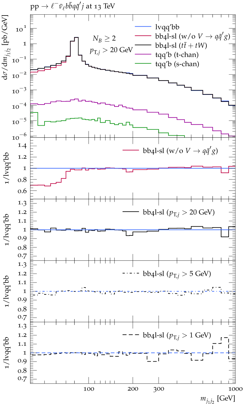
(a)

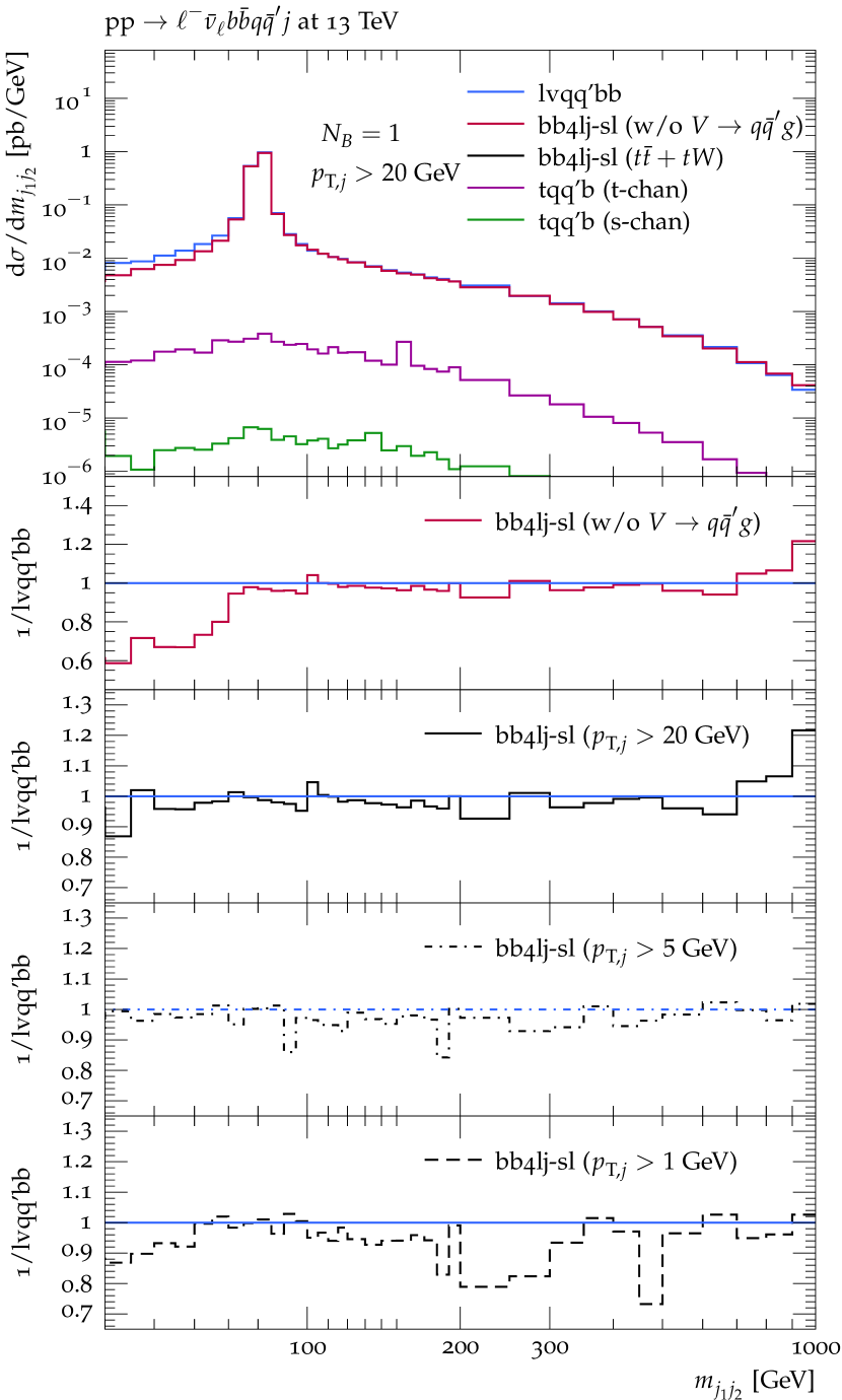
(b)

Figure 18: Distribution in the dijet invariant mass of the first two light jets for off-shell $\ell^{-}\bar{\nu}_{\ell}q\bar{q}^{\prime}b\bar{b}+$jet production at $\mathcal{O}(\alpha_{\rm S}^{3}\alpha^{4})$ in the phase space with $N_{B}\geq 2$ (18(a)) and $N_{B}=1$ (18(b)) $B$-jets. The precise definition of the dijet mass is given in the main text. Complete off-shell predictions are compared to the contributions of the most relevant subprocesses: $t\bar{t}+tW$ production (i.e. bb4l-sl) including (black) or excluding (red) radiation in the $W\to q\bar{q}^{\prime}$ decay, and $t$-channel (purple) plus $s$-channel (green) single-top production. The upper panels show absolute predictions with $p_{\mathrm{T},{\rm min}}=20$ GeV, while the three lowest panels show the ratio of bb4l-sl wrt the complete off-shell process for three different values of $p_{\mathrm{T},{\rm min}}$. The second panel shows the same ratio for bb4l-sl without radiation in the $W\to q\bar{q}^{\prime}$ decay and with $p_{\mathrm{T},{\rm min}}=20$ GeV.

In Fig. 18 we present the distribution in the dijet mass, defined as the invariant mass of the system of two or three light jets that is closest to $m_{W}$. For this observable we note that the inclusion of radiation in the $W\to q\bar{q}^{\prime}$ decay is quite relevant, especially in the region below the $W$ resonance, where it can increase the differential cross section by up to $30\%$. In general, for the dijet mass distribution and for all $p_{\mathrm{T}}$ distributions in Figs. 19–20 we find that—for all considered jet-$p_{\mathrm{T}}$ thresholds—the bb4l-sl contribution agrees with the exact off-shell cross section at the $1\%$ level. In particular, it is interesting to note that also the tail of the distribution in the $p_{\mathrm{T}}$ of the second light jet (Fig. 2020(c)–20(d)) is free from any sizeable contribution beyond the one from bb4l-sl. This is due to the fact that, thanks to the emission of NLO QCD radiation, the abrupt suppression of the $t\bar{t}+tW$ cross section observed in Fig. 1717(c)–17(d) disappears, i.e. $t\bar{t}+tW$ production can populate the phase space with two high-$p_{\mathrm{T}}$ light jets in a similarly efficient way as the single-top subprocesses.

These findings provide further evidence of the consistency of the process definition adopted for the bb4l-sl generator.

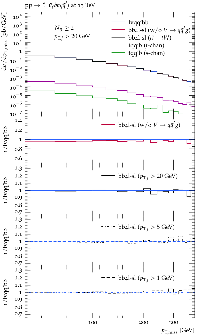
(a)

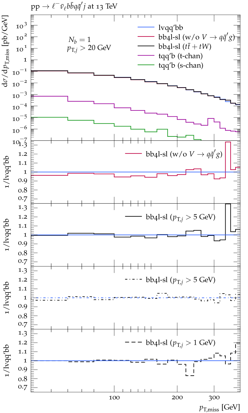
(b)

(c)

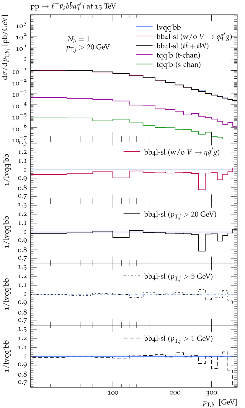
(d)

Figure 19: Same predictions and ratios as in Fig. 18 for the distributions in the missing $p_{\mathrm{T}}$ (19(a)–19(b)) and in the $p_{\mathrm{T}}$ of the first $B$-jet (20(c)–20(d)).

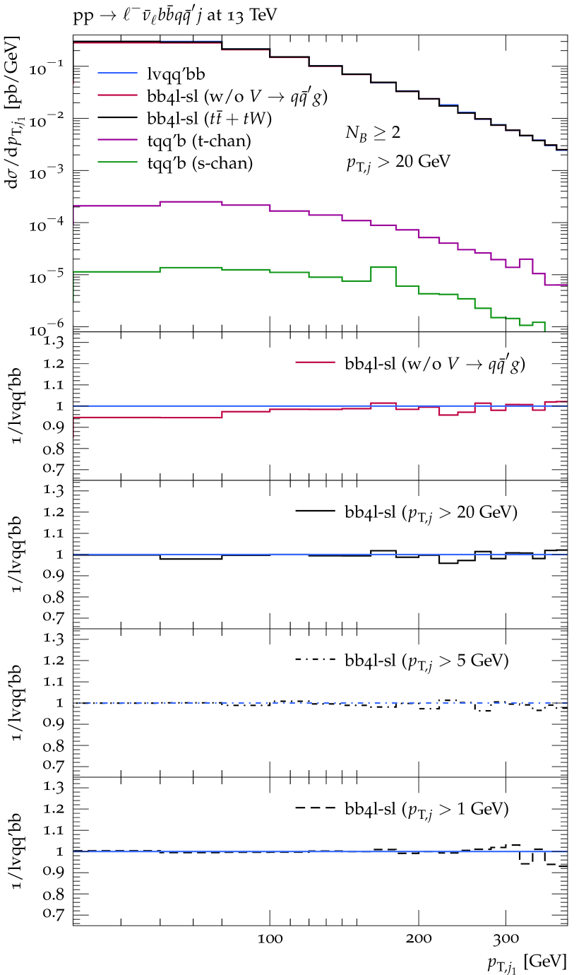
(a)

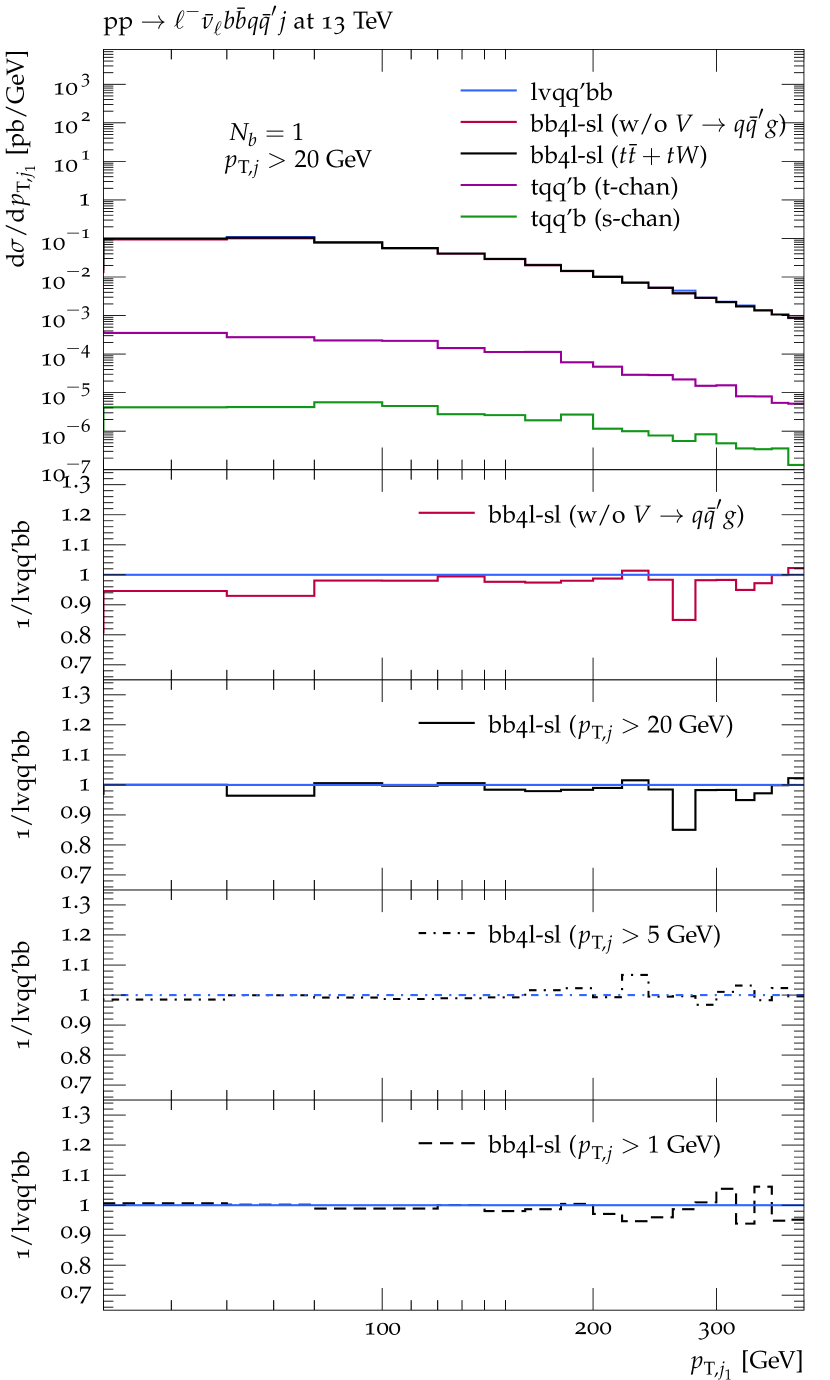
(b)

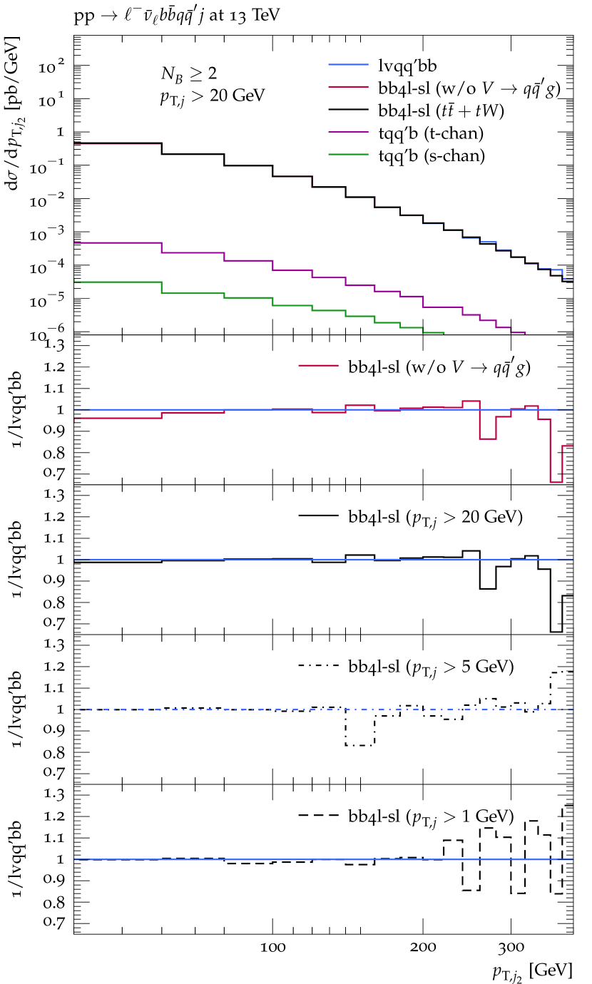
(c)

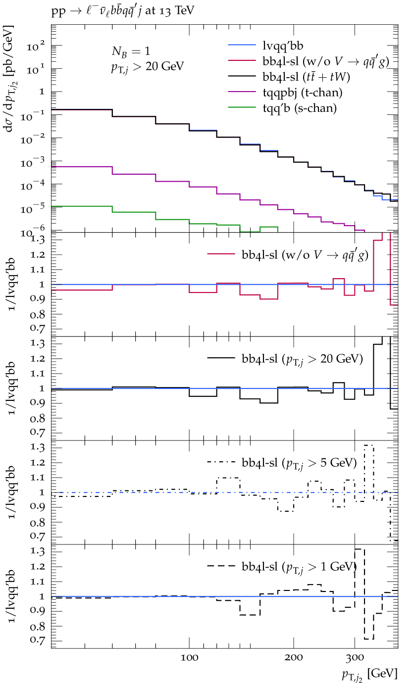
(d)

Figure 20: Same predictions and ratios as in Fig. 18 for the distributions in the $p_{\mathrm{T}}$ of the first (20(a)–20(b)) and of the second (20(c)–20(d)) light jet.

References

- (1) F. Cascioli, S. Kallweit, P. Maierhöfer, and S. Pozzorini, A unified NLO description of top-pair and associated Wt production, Eur. Phys. J. C74 (2014), no. 3 2783, [arXiv:1312.0546].
- (2) T. Ježo, J. M. Lindert, P. Nason, C. Oleari, and S. Pozzorini, An NLO+PS generator for and production and decay including non-resonant and interference effects, Eur. Phys. J. C76 (2016), no. 12 691, [arXiv:1607.04538].
- (3) S. Frixione, P. Nason, and B. R. Webber, Matching NLO QCD and parton showers in heavy flavour production, JHEP 08 (2003) 007, [hep-ph/0305252].
- (4) S. Frixione, P. Nason, and G. Ridolfi, A Positive-Weight Next-to-Leading-Order Monte Carlo for Heavy Flavour Hadroproduction, JHEP 09 (2007) 126, [arXiv:0707.3088].
- (5) J. Alwall, R. Frederix, S. Frixione, V. Hirschi, F. Maltoni, et al., The automated computation of tree-level and next-to-leading order differential cross sections, and their matching to parton shower simulations, JHEP 1407 (2014) 079, [arXiv:1405.0301].
- (6) S. Höche, F. Krauss, P. Maierhöfer, S. Pozzorini, M. Schönherr, and F. Siegert, Next-to-leading order QCD predictions for top-quark pair production with up to two jets merged with a parton shower, Phys. Lett. B748 (2015) 74–78, [arXiv:1402.6293].
- (7) K. Cormier, S. Plätzer, C. Reuschle, P. Richardson, and S. Webster, Parton showers and matching uncertainties in top quark pair production with Herwig 7, Eur. Phys. J. C 79 (2019), no. 11 915, [arXiv:1810.06493].
- (8) S. Frixione, E. Laenen, P. Motylinski, and B. R. Webber, Angular correlations of lepton pairs from vector boson and top quark decays in Monte Carlo simulations, JHEP 04 (2007) 081, [hep-ph/0702198].
- (9) P. Artoisenet, R. Frederix, O. Mattelaer, and R. Rietkerk, Automatic spin-entangled decays of heavy resonances in Monte Carlo simulations, JHEP 03 (2013) 015, [arXiv:1212.3460].
- (10) M. V. Garzelli, A. Kardos, and Z. Trocsanyi, Hadroproduction of at NLO accuracy matched with shower Monte Carlo programs, JHEP 08 (2014) 069, [arXiv:1405.5859].
- (11) S. Höche, S. Kuttimalai, S. Schumann, and F. Siegert, Beyond Standard Model calculations with Sherpa, Eur. Phys. J. C75 (2015), no. 3 135, [arXiv:1412.6478].
- (12) T. Sjostrand, S. Mrenna, and P. Z. Skands, A Brief Introduction to PYTHIA 8.1, Comput.Phys.Commun. 178 (2008) 852–867, [arXiv:0710.3820].
- (13) T. Sjöstrand, S. Ask, J. R. Christiansen, R. Corke, N. Desai, P. Ilten, S. Mrenna, S. Prestel, C. O. Rasmussen, and P. Z. Skands, An Introduction to PYTHIA 8.2, Comput. Phys. Commun. 191 (2015) 159–177, [arXiv:1410.3012].
- (14) W. Bernreuther, M. Fucker, and Z.-G. Si, Weak interaction corrections to hadronic top quark pair production: Contributions from quark-gluon and b anti-b induced reactions, Phys. Rev. D78 (2008) 017503, [arXiv:0804.1237].
- (15) J. H. Kühn, A. Scharf, and P. Uwer, Electroweak effects in top-quark pair production at hadron colliders, Eur. Phys. J. C51 (2007) 37–53, [hep-ph/0610335].
- (16) W. Hollik and D. Pagani, The electroweak contribution to the top quark forward-backward asymmetry at the Tevatron, Phys. Rev. D84 (2011) 093003, [arXiv:1107.2606].
- (17) C. Gütschow, J. M. Lindert, and M. Schönherr, Multi-jet merged top-pair production including electroweak corrections, Eur. Phys. J. C 78 (2018), no. 4 317, [arXiv:1803.00950].
- (18) R. Frederix, I. Tsinikos, and T. Vitos, Probing the spin correlations of production at NLO QCD+EW, Eur. Phys. J. C 81 (2021), no. 9 817, [arXiv:2105.11478].
- (19) M. Czakon, D. Heymes, A. Mitov, D. Pagani, I. Tsinikos, and M. Zaro, Top-pair production at the LHC through NNLO QCD and NLO EW, JHEP 10 (2017) 186, [arXiv:1705.04105].
- (20) M. Czakon, P. Fiedler, and A. Mitov, Total Top-Quark Pair-Production Cross Section at Hadron Colliders Through , Phys. Rev. Lett. 110 (2013) 252004, [arXiv:1303.6254].
- (21) M. Czakon, D. Heymes, and A. Mitov, High-precision differential predictions for top-quark pairs at the LHC, Phys. Rev. Lett. 116 (2016), no. 8 082003, [arXiv:1511.00549].
- (22) S. Catani, S. Devoto, M. Grazzini, S. Kallweit, J. Mazzitelli, and H. Sargsyan, Top-quark pair hadroproduction at next-to-next-to-leading order in QCD, Phys. Rev. D99 (2019), no. 5 051501, [arXiv:1901.04005].
- (23) S. Catani, S. Devoto, M. Grazzini, S. Kallweit, and J. Mazzitelli, Top-quark pair production at the LHC: Fully differential QCD predictions at NNLO, JHEP 07 (2019) 100, [arXiv:1906.06535].
- (24) J. Mazzitelli, P. F. Monni, P. Nason, E. Re, M. Wiesemann, and G. Zanderighi, Top-pair production at the LHC with MINNLOPS, JHEP 04 (2022) 079, [arXiv:2112.12135].
- (25) J. Mazzitelli, P. F. Monni, P. Nason, E. Re, M. Wiesemann, and G. Zanderighi, Next-to-Next-to-Leading Order Event Generation for Top-Quark Pair Production, Phys. Rev. Lett. 127 (2021), no. 6 062001, [arXiv:2012.14267].
- (26) W. Bernreuther, A. Brandenburg, Z. G. Si, and P. Uwer, Top quark pair production and decay at hadron colliders, Nucl. Phys. B690 (2004) 81–137, [hep-ph/0403035].
- (27) K. Melnikov and M. Schulze, NLO QCD corrections to top quark pair production and decay at hadron colliders, JHEP 08 (2009) 049, [arXiv:0907.3090].
- (28) J. M. Campbell and R. K. Ellis, Top-quark processes at NLO in production and decay, J. Phys. G42 (2015), no. 1 015005, [arXiv:1204.1513].
- (29) J. M. Campbell, R. K. Ellis, P. Nason, and E. Re, Top-pair production and decay at NLO matched with parton showers, JHEP 04 (2015) 114, [arXiv:1412.1828].
- (30) J. Gao, C. S. Li, and H. X. Zhu, Top Quark Decay at Next-to-Next-to Leading Order in QCD, Phys. Rev. Lett. 110 (2013), no. 4 042001, [arXiv:1210.2808].
- (31) M. Brucherseifer, F. Caola, and K. Melnikov, corrections to fully-differential top quark decays, JHEP 04 (2013) 059, [arXiv:1301.7133].
- (32) J. Gao and A. S. Papanastasiou, Top-quark pair-production and decay at high precision, Phys. Rev. D96 (2017), no. 5 051501, [arXiv:1705.08903].
- (33) A. Behring, M. Czakon, A. Mitov, A. S. Papanastasiou, and R. Poncelet, Higher order corrections to spin correlations in top quark pair production at the LHC, Phys. Rev. Lett. 123 (2019), no. 8 082001, [arXiv:1901.05407].
- (34) M. Czakon, A. Mitov, and R. Poncelet, NNLO QCD corrections to leptonic observables in top-quark pair production and decay, JHEP 05 (2021) 212, [arXiv:2008.11133].
- (35) E. Re, Single-top Wt-channel production matched with parton showers using the POWHEG method, Eur. Phys. J. C71 (2011) 1547, [arXiv:1009.2450].
- (36) S. Frixione, E. Laenen, P. Motylinski, B. R. Webber, and C. D. White, Single-top hadroproduction in association with a W boson, JHEP 07 (2008) 029, [arXiv:0805.3067].
- (37) E. Bothmann, F. Krauss, and M. Schönherr, Single top-quark production with SHERPA, Eur. Phys. J. C 78 (2018), no. 3 220, [arXiv:1711.02568].
- (38) M. Beccaria, G. Macorini, F. M. Renard, and C. Verzegnassi, Associated tW production at lhc: A Complete calculation of electroweak supersymmetric effects at one loop, Phys. Rev. D 73 (2006) 093001, [hep-ph/0601175].
- (39) M. Beccaria, C. M. Carloni Calame, G. Macorini, G. Montagna, F. Piccinini, F. M. Renard, and C. Verzegnassi, A Complete one-loop description of associated tW production at LHC and a search for possible genuine supersymmetric effects, Eur. Phys. J. C 53 (2008) 257–265, [arXiv:0705.3101].
- (40) S. Zhu, Next-to-leading order QCD corrections to at CERN large hadron collider, hep-ph/0109269.
- (41) J. M. Campbell and F. Tramontano, Next-to-leading order corrections to production and decay, Nucl. Phys. B726 (2005) 109–130, [hep-ph/0506289].
- (42) C. D. White, S. Frixione, E. Laenen, and F. Maltoni, Isolating Wt production at the LHC, JHEP 11 (2009) 074, [arXiv:0908.0631].
- (43) F. Demartin, B. Maier, F. Maltoni, K. Mawatari, and M. Zaro, tWH associated production at the LHC, Eur. Phys. J. C77 (2017), no. 1 34, [arXiv:1607.05862].
- (44) A. Denner et al., Electroweak corrections to charged-current 4 fermion processes: Technical detail results, Nucl.Phys. B724 (2005) 247–294, [hep-ph/0505042].
- (45) G. Bevilacqua, M. Czakon, A. van Hameren, C. G. Papadopoulos, and M. Worek, Complete off-shell effects in top quark pair hadroproduction with leptonic decay at next-to-leading order, JHEP 02 (2011) 083, [arXiv:1012.4230].
- (46) A. Denner, S. Dittmaier, S. Kallweit, and S. Pozzorini, NLO QCD corrections to WWbb production at hadron colliders, Phys. Rev. Lett. 106 (2011) 052001, [arXiv:1012.3975].
- (47) A. Denner, S. Dittmaier, S. Kallweit, and S. Pozzorini, NLO QCD corrections to off-shell top-antitop production with leptonic decays at hadron colliders, JHEP 10 (2012) 110, [arXiv:1207.5018].
- (48) G. Heinrich, A. Maier, R. Nisius, J. Schlenk, and J. Winter, NLO QCD corrections to production with leptonic decays in the light of top quark mass and asymmetry measurements, JHEP 06 (2014) 158, [arXiv:1312.6659].
- (49) R. Frederix, Top Quark Induced Backgrounds to Higgs Production in the Decay Channel at Next-to-Leading-Order in QCD, Phys. Rev. Lett. 112 (2014), no. 8 082002, [arXiv:1311.4893].
- (50) A. Denner and M. Pellen, Off-shell production of top-antitop pairs in the lepton+jets channel at NLO QCD, JHEP 02 (2018) 013, [arXiv:1711.10359].
- (51) A. Denner and M. Pellen, NLO electroweak corrections to off-shell top-antitop production with leptonic decays at the LHC, JHEP 08 (2016) 155, [arXiv:1607.05571].
- (52) G. Bevilacqua, H. B. Hartanto, M. Kraus, and M. Worek, Top Quark Pair Production in Association with a Jet with Next-to-Leading-Order QCD Off-Shell Effects at the Large Hadron Collider, Phys. Rev. Lett. 116 (2016), no. 5 052003, [arXiv:1509.09242].
- (53) T. Ježo and P. Nason, On the Treatment of Resonances in Next-to-Leading Order Calculations Matched to a Parton Shower, JHEP 12 (2015) 065, [arXiv:1509.09071].
- (54) P. Nason, A new method for combining NLO QCD with shower Monte Carlo algorithms, JHEP 11 (2004) 040, [hep-ph/0409146].
- (55) S. Frixione, P. Nason, and C. Oleari, Matching NLO QCD computations with Parton Shower simulations: the POWHEG method, JHEP 11 (2007) 070, [arXiv:0709.2092].
- (56) S. Frixione and B. R. Webber, Matching NLO QCD computations and parton shower simulations, JHEP 06 (2002) 029, [hep-ph/0204244].
- (57) R. Frederix, S. Frixione, A. S. Papanastasiou, S. Prestel, and P. Torrielli, Off-shell single-top production at NLO matched to parton showers, arXiv:1603.01178.
- (58) ATLAS Collaboration, M. Aaboud et al., Probing the quantum interference between singly and doubly resonant top-quark production in collisions at TeV with the ATLAS detector, Phys. Rev. Lett. 121 (2018), no. 15 152002, [arXiv:1806.04667].
- (59) ATLAS Collaboration, Studies of interference effects in final states with Powheg and MG5_aMC@NLO setups, .
- (60) ATLAS Collaboration, Measurement of the top-quark mass in dilepton events with the ATLAS experiment using the template method in 13 TeV collision data, .
- (61) C. Herwig, T. Ježo, and B. Nachman, Extracting the Top-Quark Width from Nonresonant Production, Phys. Rev. Lett. 122 (2019), no. 23 231803, [arXiv:1903.10519].
- (62) S. Ferrario Ravasio, T. Ježo, P. Nason, and C. Oleari, A theoretical study of top-mass measurements at the LHC using NLO+PS generators of increasing accuracy, Eur. Phys. J. C 78 (2018), no. 6 458, [arXiv:1906.09166]. [Addendum: Eur.Phys.J.C 79, 859 (2019)].
- (63) F. Cascioli, P. Maierhöfer, and S. Pozzorini, Scattering Amplitudes with Open Loops, Phys.Rev.Lett. 108 (2012) 111601, [arXiv:1111.5206].
- (64) F. Buccioni, S. Pozzorini, and M. Zoller, On-the-fly reduction of open loops, Eur. Phys. J. C78 (2018), no. 1 70, [arXiv:1710.11452].
- (65) F. Buccioni, J.-N. Lang, J. M. Lindert, P. Maierhöfer, S. Pozzorini, H. Zhang, and M. F. Zoller, OpenLoops 2, Eur. Phys. J. C 79 (2019), no. 10 866, [arXiv:1907.13071].
- (66) W. Hollik, J. M. Lindert, and D. Pagani, NLO corrections to squark-squark production and decay at the LHC, JHEP 03 (2013) 139, [arXiv:1207.1071].
- (67) R. V. Harlander, S. Y. Klein, and M. Lipp, FeynGame, Comput. Phys. Commun. 256 (2020) 107465, [arXiv:2003.00896].
- (68) S. Alioli, P. Nason, C. Oleari, and E. Re, NLO Higgs boson production via gluon fusion matched with shower in POWHEG, JHEP 0904 (2009) 002, [arXiv:0812.0578].
- (69) T. Ježo, J. M. Lindert, N. Moretti, and S. Pozzorini, New NLOPS predictions for -jet production at the LHC, Eur. Phys. J. C78 (2018), no. 6 502, [arXiv:1802.00426].
- (70) K. Kondo, Dynamical Likelihood Method for Reconstruction of Events With Missing Momentum. 1: Method and Toy Models, J. Phys. Soc. Jap. 57 (1988) 4126–4140.
- (71) E. Boos, M. Dobbs, W. Giele, I. Hinchliffe, J. Huston, et al., Generic user process interface for event generators, hep-ph/0109068.
- (72) A. Denner, S. Dittmaier, M. Roth, and D. Wackeroth, Predictions for all processes 4 fermions + , Nucl. Phys. B560 (1999) 33–65, [hep-ph/9904472].
- (73) NNPDF Collaboration, R. D. Ball et al., Parton distributions from high-precision collider data, Eur. Phys. J. C 77 (2017), no. 10 663, [arXiv:1706.00428].
- (74) A. Buckley, J. Ferrando, S. Lloyd, K. Nordström, B. Page, M. Rüfenacht, M. Schönherr, and G. Watt, LHAPDF6: parton density access in the LHC precision era, Eur. Phys. J. C75 (2015) 132, [arXiv:1412.7420].
- (75) M. Cacciari, M. Greco, and P. Nason, The spectrum in heavy flavor hadroproduction, JHEP 9805 (1998) 007, [hep-ph/9803400].
- (76) A. Buckley, J. Butterworth, L. Lönnblad, D. Grellscheid, H. Hoeth, J. Monk, H. Schulz, and F. Siegert, Rivet user manual, Comput. Phys. Commun. 184 (2013) 2803–2819, [arXiv:1003.0694].
- (77) M. Cacciari, G. P. Salam, and G. Soyez, The anti- jet clustering algorithm, JHEP 04 (2008) 063, [arXiv:0802.1189].
- (78) S. Alioli, P. Nason, C. Oleari, and E. Re, A general framework for implementing NLO calculations in shower Monte Carlo programs: the POWHEG BOX, JHEP 06 (2010) 043, [arXiv:1002.2581].
- (79) Sherpa Collaboration, E. Bothmann et al., Event Generation with Sherpa 2.2, SciPost Phys. 7 (2019), no. 3 034, [arXiv:1905.09127].