Distinct photon-ALP propagation modes

Abstract

The detection of ultra high energy gamma-rays provides an opportunity to explore the existence of ALPs at the multi-hundred TeV and PeV energy scales. We discover that we can employ analytic methods to investigate the propagation of photon-ALP beams in scenarios where the energy of photons $\omega\geq 100$ TeV. Our analytical calculations uncover the presence of two distinct modes of photon propagation resulting from the interplay between ALP-photon mixing and attenuation effects. Next, we analyze observable quantities such as the degree of polarization and survival probability in these two modes. We determine the conditions under which a significant polarization effect can be observed and identify the corresponding survival probability. Finally, we extend our analytic methods to cover the energy range of $10^{-3}$ to $10^{4}$ GeV and analyze the influence of ALPs on the experimental signals.

1 Introduction

The existence of axions and axion-like particles (ALPs) is a topic of great interest in modern particle physics Ringwald:2012hr ; Irastorza:2018dyq ; Adams:2022pbo . The QCD axion was initially proposed as a natural solution to the strong CP problem Peccei:1977hh ; Wilczek:1977pj . Recently, the study of ALPs has gained widespread attention due to the much wider range of mass and coupling parameter than the QCD axion Jaeckel:2010ni . ALPs arise naturally in a plethora of extensions of the standard model, including supersymmetric models Chang:1999si ; Turok:1995ai and superstring theories Svrcek:2006yi ; Ringwald:2008cu ; Arvanitaki:2009fg .

The presence of ALPs can significantly alter photon propagation in the universe, leading to distinct photon-ALP oscillation signatures Maiani:1986md ; Raffelt:1987im . Therefore, it is of importance to study their propagation properties. Because of the complex astrophysical environment through which photon-ALP beams propagate, most studies employ numerical simulations to analyze their propagation properties Li:2020pcn ; Horns:2012pp ; Gill:2011yp ; Bi:2020ths ; Galanti:2022yxn ; Galanti:2022tow ; Xia:2019yud ; Liang:2018mqm . In this study we take a unique approach to solve the ALP-photon propagation problem by making reasonable assumptions, which allows us to use analytic methods to study the propagation of photon-ALP beams in the Milky Way (MW) galaxy and beyond. Our analytic approach offers a complementary perspective that provides insight into the fundamental physics of photon-ALP interactions.

Our analytic methods reveal two distinct photon propagation modes, characterized by the sign of the quantity $D$, which is defined in Eq. (14). We find that in the $D>0$ case, photons exhibit clear oscillations during the propagation; conversely, in the $D<0$ case, the oscillations are absent. We investigate the astrophysical conditions that lead to the emergence of these two propagation modes, and further study the implications for relevant physical observables such as the photon survival probability and degree of polarization. We study the distinguishing features of the two propagation modes in detail, which can be used to discriminate between the two modes, as well as against the standard model background.

The rest of paper is organized as follows. In section 2, we introduce the ALPs and the propagation equation governing the photon-ALP system. In section 3, we introduce the two distinct photon propagation modes that are characterized by the sign of a quantity $D$. We compute the density matrix via analytic methods and further discuss the effects of ALPs on the density matrix. In sections 4 and 5, we discuss the physical observables such as the photon survival probability and the photon degree of polarization in the two propagation modes: We focus on photons with energies above 100 TeV in section 4, and photons with energies in the range of $10^{-3}-10^{4}$ GeV in section 5. In section 6, we summarize our findings. In the appendix, we compare our analytic method in which a uniform magnetic field is assumed, with numerical calculations in which magnetic field models that aim to describe the astrophysical conditions are used.

2 Propagation Equation

Consider the following effective interaction Lagrangian between the axion-like particle (ALP) $a$ and the photon

$$\mathcal{L}_{\rm int}=-\frac{1}{4}g_{a\gamma}F^{\mu\nu}\tilde{F}_{\mu\nu}\,a=g_{a\gamma}\mathbf{E}\cdot\mathbf{B}\,a,$$ (1)

where $F^{\mu\nu}$ is the electromagnetic stress tensor and $\tilde{F}_{\mu\nu}$ is the dual, $\mathbf{E}$ and $\mathbf{B}$ are the electric and magnetic fields, respectively, and $g_{a\gamma}$ is the coupling constant.

The propagation of the photon-ALP beam along the $z$-direction with energy $\omega$ can be described by a three-component vector $\psi=(A_{x},A_{y},a)^{T}$, where $A_{x}$ and $A_{y}$ are the electromagnetic potentials linearly polarized along the $x$ and $y$ axes, respectively. Without loss of generality, we consider the case where the external magnetic field is along the $y$ direction and the equation that governs the propagation of $\psi$ is given by Raffelt:1987im ; DeAngelis:2011id ,

$$\left(i\frac{d}{dz}+\omega+\mathcal{M}\right)\psi=0,$$ (2)

where $\mathcal{M}$ is given by

$$\mathcal{M}=\begin{pmatrix}\Delta_{x}&0&0\\ 0&\Delta_{y}&\Delta_{a\gamma}\\ 0&\Delta_{a\gamma}&\Delta_{aa}\end{pmatrix}+\begin{pmatrix}i\Gamma&0&0\\ 0&i\Gamma&0\\ 0&0&0\end{pmatrix}.$$ (3)

Here, $\Delta_{x}$ and $\Delta_{y}$ describe the medium effects, $\Gamma$ is the absorption rate accounting for the attenuation of photons, $\Delta_{a\gamma}=g_{a\gamma}B/2$ is the photon-ALP mixing term with $B=|\boldsymbol{B}|$, and $\Delta_{aa}=-m_{a}^{2}/(2\omega)$ with $m_{a}$ being the ALP mass. The absorption rate $\Gamma$ is mainly caused by the reaction $\gamma\gamma\to e^{+}e^{-}$ between the propagating photons and ambient photons, such as cosmic microwave background, extragalactic background light, and so on Vernetto:2016alq ; Lipari:2018gzn . As shown in the black line of Fig. (1), $\Gamma$ becomes significant as energy $\omega\gtrsim 100$ TeV.

The medium effects are given by

$$\Delta_{x,y}=N\Delta_{\rm QED}+\Delta_{\rm pl}+\Delta_{\rm dis},$$ (4)

where $N=2$ $(7/2)$ for $\Delta_{x}$ ($\Delta_{y}$), $\Delta_{\rm QED}$ represents the QED birefringence, $\Delta_{\rm pl}$ represents the plasma effect, and $\Delta_{\rm dis}$ accounts for dispersion effects from photon-photon scattering on environmental radiation field Bi:2020ths ; Galanti:2022yxn . The plasma effect $\Delta_{\rm pl}$ is given by

$$\Delta_{\rm pl}=-\frac{\omega_{\rm pl}^{2}}{2\omega}=-\frac{e^{2}n_{e}}{2m_{e}\omega},$$ (5)

where $\omega_{\rm pl}$ is the plasma frequency, $e$ is the QED coupling, and $m_{e}$ and $n_{e}$ is the mass and number density of the electron, respectively. For the case of $\omega\lesssim 100\ \text{TeV}$, the QED birefringence and dispersion effects can be obtained from the Euler-Heisenberg Lagrangian Dittrich:2000zu ; Latorre:1994cv ; Cougo-Pinto:1999agw ; Tarrach:1983cb ; Adler:1971wn

$$\Delta_{\rm QED} =\frac{\alpha\omega}{45\pi}\left(\frac{Be}{m_{e}^{2}}\right)^{2},$$ (6)

$$\Delta_{\rm dis} =\frac{44\alpha^{2}\rho_{\rm RF}\omega}{135m_{e}^{4}},$$ (7)

where $\alpha$ is the fine structure constant, and $\rho_{\rm RF}$ is the ambient photon energy density. For the high energy cosmic gamma-ray with $\omega\gtrsim\omega_{2}=100$ TeV, Euler-Heisenberg approximation breaks down, and one can use the a scaling function $g_{2}(\omega/\omega_{2})$ to take into account the gamma-gamma scattering due to background photon Dobrynina:2014qba . Thus, at photon energy $\omega\gtrsim\omega_{2}=100$ TeV, the quantities $\Delta_{\rm QED}$ and $\Delta_{\rm dis}$ are both modified to $\Delta_{\rm QED(dis)}g_{2}(\omega/\omega_{2})$, as follows Dobrynina:2014qba :

$$\begin{split}g_{2}(u)&=\frac{15}{\pi^{4}}\int_{0}^{\infty}dx\frac{x^{3}}{e^{x}-1}g_{1}\left(ux\frac{30\zeta(3)}{\pi^{4}}\right),\\ g_{1}(u)&=\frac{3}{8}\int^{+1}_{-1}d\mu(1-\mu)^{2}g_{0}\left(u\frac{1-\mu}{2}\right),\\ g_{0}(u)&=\frac{45}{44}\int_{1}^{\infty}du^{\prime}\frac{f(u^{\prime})}{u^{\prime 2}-u^{2}},\\ f(u)&=\frac{4u(u+1)-2}{u^{3}}\ln(\sqrt{u}+\sqrt{u-1})-\frac{2(u+1)\sqrt{u-1}}{u^{5/2}}.\end{split}$$ (8)

Note that Eq. (2) is similar to the Schrödinger equation if the coordinate $z$ is replaced by the time $t$ and $(\omega+{\cal M})$ is replaced by $-\mathcal{H}$, where $\mathcal{H}$ denotes the Hamiltonian. Thus, analogous to solving the Schrödinger equation, one can also construct the transition matrix $U(z)=e^{i\mathcal{M}z}$ for the photon-ALP progapation. For a more general case, one can define the density matrix $\rho\equiv\psi\psi^{\dagger}$, which satisfies an equation similar to the Von Neumann equation,

$$i\frac{d}{dz}\rho=\rho\mathcal{M}^{\dagger}-\mathcal{M}\rho.$$ (9)

The solution can then be obtained via $\rho(z)=U(z)\rho_{0}U(z)^{\dagger}$, where $\rho_{0}$ is the initial condition. In our analysis, we assume an unpolarized photon beam such that $\rho_{0}=\text{diag}(1/2,1/2,0)$. The upper-left $2\times 2$ submatrix of $\rho$, denoted as $\rho_{\gamma}$, can be parameterized as Kosowsky:1998mb

$$\rho_{\gamma}=\begin{pmatrix}\rho_{x}&\rho_{xy}\\ \rho_{xy}^{*}&\rho_{y}\end{pmatrix}=\frac{1}{2}\begin{pmatrix}I+Q&U-iV\\ U+iV&I-Q\end{pmatrix},$$ (10)

where $I$, $Q$, $U$, and $V$ are the Stokes parameters. The photon degree of polarization $\Pi_{L}$ is then given by defin

$$\Pi_{L}=\frac{\sqrt{Q^{2}+U^{2}}}{I}.$$ (11)

The photon survival probability after propagation is given by DeAngelis:2011id

$$P_{\gamma\to\gamma}=\rho_{x}+\rho_{y}=I.$$ (12)

3 Two Different Propagation Modes

Because of the medium effects and the magnetic field configurations in the Milky Way (and in other galaxies) can be rather complicated, the propagation of the photon-ALP beam in these astrophysical systems is usually solved numerically; see e.g., Refs. Li:2020pcn ; Horns:2012pp ; Gill:2011yp ; Bi:2020ths ; Galanti:2022yxn ; Galanti:2022tow ; Xia:2019yud ; Liang:2018mqm . However, there are instances where analytic calculations are good approximations to the photon propagation. In this section, we first identify the conditions in which simple analytic solutions to the photon propagation can be obtained, and then discuss two different propagation modes shown in the analytic calculations.

We are interested in the very high energy photons with $\omega\gtrsim 100$ TeV. At such high energy, the matrix $\cal M$ can be greatly simplified, because the various $\Delta$ terms can be neglected except the new physics term $\Delta_{a\gamma}$ and the absorption term $\Gamma$, as shown in Fig. (1), where $g_{a\gamma}=3\times 10^{-12}\ \text{GeV}^{-1}$ and $B=2\ \mu$G are assumed. Thus we have

$$\mathcal{M}\simeq\begin{pmatrix}i\Gamma&0&0\\ 0&i\Gamma&\frac{1}{2}g_{a\gamma}B\\ 0&\frac{1}{2}g_{a\gamma}B&0\end{pmatrix}.$$ (13)

We further assume that the variation of external magnetic field is relatively small so that it can be approximated by a uniform magnetic field. In this case, one can then analytically solve the propagation. We note that the analytical solution can facilitate the calculations and can reveal some physics pictures of the problem that are difficult to be seen in the numerical calculations.

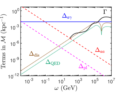
Figure 1: Matrix elements of $\mathcal{M}$ as a function of the photon energy $\omega$. Here we take $g_{a\gamma}=3\times 10^{-12}\ \text{GeV}^{-1}$, $B=2\ \mu$G, $m_{a}=1\times 10^{-19}\ \text{GeV}$, $n_{e}=1.1\times 10^{-2}\ \text{cm}^{-3}$ accounting for the electron number density in the Milky Way JMYAO and $\rho_{\rm RF}=2.01\times 10^{-51}\ \text{GeV}^{4}$. accounting for the energy density of CMB Dobrynina:2014qba . We use Eq. (6) and Eq. (7) to compute $\Delta_{\rm QED}$ and $\Delta_{\rm dis}$; for $\omega>$100 TeV, we further multiply a factor of $g_{2}(\omega/\omega_{2})$ where $\omega_{2}=100$ TeV given in Ref. Dobrynina:2014qba . The $\Gamma$ curve is adopted from Ref. Lipari:2018gzn .

We then find that in the analytic solutions for the simplified $\cal M$, there exist two different propagation modes of photons, characterized by the sign of $D$, which is defined as

$$D\equiv g_{a\gamma}^{2}B^{2}-\Gamma^{2}.$$ (14)

We discuss these two propagation modes: $D>0$ and $D<0$ below.

3.1 The $D>0$ propagation mode

We first discuss the $D>0$ case. To solve the propagation analytically, we first compute the transition matrix $U(z)=e^{i\mathcal{M}z}$, where $\mathcal{M}$ is given by Eq. (13). Thus, for the $D>0$ case, we have

$$U_{D>0}(z)=\frac{e^{-\frac{\Gamma}{2}z}}{\cos\varphi}\begin{pmatrix}e^{-\frac{\Gamma}{2}z}\cos{\varphi}&0&0\\ 0&\cos\left(\varphi+\frac{\Delta}{2}z\right)&i\sin\frac{\Delta}{2}z\\ 0&i\sin\frac{\Delta}{2}z&\cos\left(\varphi-\frac{\Delta}{2}z\right)\end{pmatrix},$$ (15)

where we have defined $\Delta=\sqrt{D}$ and $\varphi=\arctan(\Gamma/\Delta)$. We then compute $\rho(z)$ at distance $z$ from the source via $\rho(z)=U(z)\rho_{0}U(z)^{\dagger}$, where $\rho_{0}=\text{diag}(1/2,1/2,0)$ is initial condition for an unpolarized photon beam at the source. The matrix elements of $\rho_{\gamma}(z)$ in this case are given by

$$\rho_{x}(z) =\frac{1}{2}e^{-2\Gamma z},$$ (16)

$$\rho_{y}(z) =\frac{1}{2}\frac{e^{-{\Gamma}z}}{\cos^{2}\varphi}\cos^{2}\left(\varphi+\frac{\Delta}{2}z\right),$$ (17)

$$\rho_{xy}(z) =0.$$ (18)

Here $\rho_{x}(z)$ and $\rho_{y}(z)$ describe the intensities of photons polarized along $x$ and $y$ directions, respectively. Because the off-diagonal element $\rho_{xy}(z)$ vanishes in this case, the photon degree of polarization $\Pi_{L}$ becomes

$$\Pi_{L}=\frac{|\rho_{x}-\rho_{y}|}{\rho_{x}+\rho_{y}}.$$ (19)

We note that the intensities of photons with polarization along the $x$ and $y$ directions exhibit different dependencies on the propagation distance $z$. We discuss the distinct behaviors below.

First, the intensity of photons polarized along the $y$ direction depends both on the attenuation term $\Gamma$ and on the ALP-interaction term $\Delta_{a\gamma}$ (through $\Delta$ and $\varphi$), but the intensity along the $x$ direction depends on $\Gamma$ only. This discrepancy arises from the fact that the external magnetic field is taken to be along the $y$ direction so that photons polarized along the $x$ direction are not directly affected by the ALP.

Second, the intensity of photons polarized along the $x$ direction decreases exponentially as the distance $z$ increases, with a decay length of $L_{d}=(2\Gamma)^{-1}$, as shown in Eq. (16). On the other hand, the intensity for photons polarized along the $y$ direction appears to exhibit a longer decay length of $L_{d}=\Gamma^{-1}$ (twice of that along the $x$ direction), based solely on the argument of the exponential function in Eq. (17). This change on the decay length is due to the fact that photons polarized along the $y$ direction can convert into ALPs that do not experience the photon attenuation effects $\Gamma$. We emphasize that the actual decay length for photons polarized along the $y$ direction will deviate somewhat from the value of $L_{d}=\Gamma^{-1}$ due to the additional $z$-dependence in Eq. (17). Specifically, taking the limit $g_{a\gamma}\to 0$ in Eq. (17) introduces an additional exponential factor $e^{-\Gamma z}$, which must be taken into account.

Third, the intensity of photons polarized along the $y$ direction, while propagating, exhibits an oscillatory behavior. We define the oscillation length, denoted by $L_{o}$, as the period of the absolute value of the cosine function in Eq. (17). The oscillation length is given by

$$L_{o}=\frac{2\pi}{\Delta}=\frac{2\pi}{\sqrt{g_{a\gamma}^{2}B^{2}-\Gamma^{2}}}.$$ (20)

Thus, the increase in the difference between $g_{a\gamma}B$ and $\Gamma$ leads to an increase in the oscillation length. We note that the oscillation is attenuated by the exponential factor $e^{-\Gamma z}$.

3.2 The $D<0$ propagation mode

We next discuss the $D<0$ case. For the case of $D<0$, the transition matrix $U(z)$ can be written as

$$U_{D<0}(z)=\frac{e^{-\frac{\Gamma}{2}z}}{\cos 2\alpha}\begin{pmatrix}e^{-\frac{\Gamma}{2}z}\cos 2\alpha&0&0\\ 0&e^{-\frac{\Delta}{2}z}\cos^{2}\alpha-e^{\frac{\Delta}{2}z}\sin^{2}\alpha&i\left(e^{\frac{\Delta}{2}z}-e^{-\frac{\Delta}{2}z}\right)\sin\alpha\cos\alpha\\ 0&i\left(e^{\frac{\Delta}{2}z}-e^{-\frac{\Delta}{2}z}\right)\sin\alpha\cos\alpha&e^{\frac{\Delta}{2}z}\cos^{2}\alpha-e^{-\frac{\Delta}{2}z}\sin^{2}\alpha\end{pmatrix},$$ (21)

where $\Delta=\sqrt{-D}$ and $\alpha=\arcsin{\sqrt{\Gamma-\Delta}}/{\sqrt{2\Gamma}}$.

For an unpolarized photon beam at the source, the diagonal matrix elements of $\rho_{\gamma}(z)$ are given by

$$\rho_{x}(z) =\frac{1}{2}e^{-2\Gamma z},$$ (22)

$$\rho_{y}(z) =\frac{1}{2}\frac{e^{-{\Gamma}z}}{\cos^{2}(2\alpha)}e^{-{\Delta}z}\left|\cos^{2}\alpha-e^{\Delta z}\sin^{2}\alpha\right|^{2},$$ (23)

$$\rho_{xy}(z) =0.$$ (24)

We note that both $\rho_{x}(z)$ and $\rho_{xy}(z)$ are the same as in the $D>0$ case. Similarly to the $D>0$ case, the vanishing off-diagonal element $\rho_{xy}(z)$ leads to a simplified expression of the photon as given in Eq. (19). We next discuss the distinct dependencies on the propagation distance $z$ of the intensities of photons with polarization along the $x$ and $y$ directions, and also make comparison to the $D>0$ case.

First, photons polarized along the $x$ direction only undergo attenuation characterized by the photon attenuation coefficient $\Gamma$, whereas photons polarized along the $y$ direction are influenced both by $\Gamma$ and by the mixing term with the ALP. This is similar to the $D>0$ case.

Second, the ALP-photon mixing term weakens the photon attenuation. This can be seen from the argument of the exponential function in Eq. (23), which hints a decay length of $L_{d}=(\Gamma+\Delta)^{-1}$ for $y$-polarized photons. The decay length of $x$-polarized photons is $L_{d}=(2\Gamma)^{-1}$. Since $\Delta<\Gamma$, photons polarized along the $y$-direction has a larger decay length than photons polarized along the $x$-direction. The reason behind this is the same as the $D>0$ case: when propagating, $y$-polarized photons can convert into ALPs which are unaffected by photons attenuation effects.

Third, in contrast to the $D>0$ scenario, where photons polarized in the $y$ direction exhibit oscillations, photons in the $D<0$ scenario do not exhibit any oscillatory behavior.

4 Propagation modes for high-energy photons with $\omega\geq 100$ TeV

In this section, we discuss the propagation modes for photons with energy $\omega\geq 100$ TeV. We will adopt the value of the coupling constant $g_{a\gamma}=3\times 10^{-12}$ GeV^-1 Irastorza:2021tdu as the default value for all subsequent analyses, unless otherwise stated.

In the Milky Way (MW) galaxy, the strength of the magnetic field is of $O(1)\ \mu$G Jansson:2012pc ; Jansson:2012rt . Taking $B=1\ \mu$G , we find that $Bg_{a\gamma}\simeq 0.01$ kpc^-1; equating $Bg_{a\gamma}$ with $\Gamma$ leads to the photon energy at $\sim 250$ TeV. Thus, the photon propagation mode is the $D<0$ mode for $\omega\gtrsim 250$ TeV, and the $D>0$ mode for $\omega\lesssim 250$ TeV.

For active galactic nuclei, galaxy clusters, and extragalactic space, the typical magnetic field strengths are $O(1-10^{5})\ \mu$G Pudritz:2012xj ; Tavecchio:2009zb , $O(1-10)\ \mu$G Govoni:2004as , and $O(10^{-7}-1)$ nG Neronov:2010gir ; Pshirkov:2015tua , respectively. Because the magnetic field in active galactic nuclei and galaxy clusters is typically much larger than that in the MW galaxy, the propagation mode is expected to be $D>0$ for photons with energy $\omega\geq 100$ TeV. On the other hand, the magnetic field in extragalactic space is much smaller than that in the MW galaxy, leading to the $D<0$ mode for photons with energy $\omega\geq 100$ TeV.

We note that our general discussions here are not applicable in extreme environments where the magnitude of the magnetic field and/or electron number density is significantly large such that the terms $\Delta_{\rm QED}$ and/or $\Delta_{\rm pl}$ in the $\mathcal{M}$ matrix can become substantial.

4.1 The $D>0$ case

We first discuss the physics in the $D>0$ case. For the $D>0$ mode, we first compute the photon degree of polarization $\Pi_{L}$, which is given by Eq. (19), in the absence of the off-diagonal elements of the $\rho_{\gamma}$ matrix. Due to the interaction with the ALP, photons observed at Earth can be fully polarized, i.e., $\Pi_{L}=1$, in spite of the unpolarized initial condition at the source position. This is a remarkable signature for ALP detection. Thus, it is of great interest to determine under what conditions photons observed can be fully polarized. The nearly fully-polarized $\Pi_{L}\sim 1$ can be achieved in two cases: (1) $\rho_{x}\gg\rho_{y}$, (2) $\rho_{x}\ll\rho_{y}$.

We first discuss the $\rho_{x}\gg\rho_{y}$ case. Since $\rho_{x}(z)>0$, the full-polarization case $\Pi_{L}=1$ can be achieved if $\rho_{y}(z)=0$; by using the analytic expression of $\rho_{y}(z)$ given in Eq. (17), we obtain the $z$ values for $\Pi_{L}=1$:

$$z_{n}=\frac{2}{\Delta}\left[\frac{n-1}{2}\pi+\arctan\left(\frac{\Delta}{\Gamma}\right)\right],$$ (25)

where $n$ is a positive odd integer. Thus, the full-polarization $\Pi_{L}=1$ phenomena are evenly distributed in space, and the distance between adjacent $\Pi_{L}$ points is $2\pi/\Delta$. Because $\rho_{x}(z)>0$ decreases with $z$, the detection should be performed with the smallest distance $z_{1}$ in Eq. (25), if possible. Note that $z_{1}=2\arctan(\Delta/\Gamma)/\Delta$ can be significantly small if $g_{a\gamma}B$ is sufficiently large.

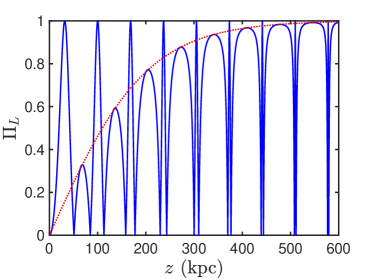
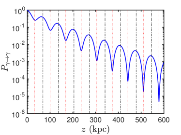
Figure 2: The photon polarization degree $\Pi_{L}$ (left) and the photon survival probability $P_{\gamma\to\gamma}$ (right) as a function of the propagation distance $z$ (blue-solid), in the $D>0$ case. Here $B=10\ \mu\text{G}$, $g_{a\gamma}=3\times 10^{-12}\ \text{GeV}^{-1}$, and $\Gamma=0.01\ \text{kpc}^{-1}$. The approximated expression of $\Pi_{L}$ given in Eq. (27) is also shown (red-dotted).

Fig. (2) shows the photon polarization degree $\Pi_{L}$ as a function of the propagation distance $z$, where a constant external magnetic field $B=10\ \mu\text{G}$, the coupling constant $g_{a\gamma}=3\times 10^{-12}\ \text{GeV}^{-1}$, and the absorption rate $\Gamma=0.01\ \text{kpc}^{-1}$ (corresponding to $\omega\sim 250$ TeV) are used. We note that in Fig. (2), $z_{1}\simeq 31.8$ kpc, and the distance between adjacent peaks in the $\rho_{x}\gg\rho_{y}$ case is $2\pi/\Delta\simeq 68.3$ kpc.

We next discuss the $\rho_{x}\ll\rho_{y}$ case. Because the $y$-polarized photons have a longer decay length than the $x$-polarized photons, eventually $\rho_{x}$ can become much smaller than $\rho_{y}$, leading to a nearly full-polarization, $\Pi_{L}\simeq 1$. By using the analytic expressions given in Eq. (16) and Eq. (17), we obtain the maximum values of $\Pi_{L}$ in the $\rho_{x}\ll\rho_{y}$ case

$$\Pi_{L}^{n}=\tanh\left(\frac{\Gamma}{2}z_{n}\right),\,\,\text{with}\,\,z_{n}=\frac{\pi n}{\Delta},$$ (26)

where $n$ is a positive even integer. Unlike the $\rho_{x}\gg\rho_{y}$ case, where $\Pi_{L}=1$ can occur at relatively small distance, in the $\rho_{x}\ll\rho_{y}$ case, large $\Pi_{L}$ only occurs at large distance; for example, in Fig. (2), the maximum value of $\Pi_{L}$ in the $\rho_{x}\ll\rho_{y}$ case is rather small ($\Pi_{L}<0.77$) until it reaches the third maximum point in this case, which is $z_{6}=6\pi/\Delta\simeq 205$ kpc.

We further extrapolate the maximum value of $\Pi_{L}$ on $z_{n}$, as given in Eq. (26), to all $z$ values,

$$\Pi_{L}=\tanh\left(\frac{\Gamma}{2}z\right),$$ (27)

which can be interpreted as the theoretical upper bound of $\Pi_{L}$, as shown in Fig. (2). It is interesting to note that Eq. (27) is independent of the external magnetic field.

We further discuss the photon survival probability. Fig. (2) shows the photon survival probability $P_{\gamma\to\gamma}$ as a function of the propagation distance $z$, for the same parameters as in Fig. (2). Because of the attenuation term $\Gamma$, the photon survival probability decreases with the propagation distance. Moreover, the presence of the ALP results in an oscillatory behavior in the photon survival probability. The photon survival probability $P_{\gamma\to\gamma}$ is bounded from above by $P_{\gamma\to\gamma}<(e^{-2\Gamma z}+e^{-\Gamma z}/\cos\phi)/2$, which is larger than the case without ALP, $P_{\gamma\to\gamma}=e^{-2\Gamma z}$. Thus, the presence of ALP makes distant galaxies brighter, resulting in a better detection probability.

As shown in Fig. (2), $\Pi_{L}\sim 1$ can occur at large $z$ values both in the $\rho_{x}\gg\rho_{y}$ case (odd-numbered peaks) and in the $\rho_{x}\ll\rho_{y}$ case (even-numbered peaks). However, as shown in Fig. (2), the photon survival probability at odd-numbered peaks can be several-order-of-magnitude smaller than the adjacent even-numbered peaks at large $z$ values. Thus, photons emitted from a distant source are likely to be observed in the $\rho_{x}\ll\rho_{y}$ case than the $\rho_{x}\gg\rho_{y}$ case.

4.2 The $D<0$ case

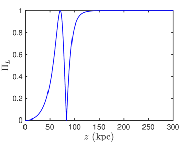
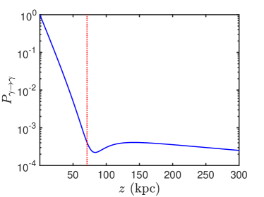
Figure 3: The photon polarization degree $\Pi_{L}$ (left) and the photon survival probability $P_{\gamma\to\gamma}$ (right) as a function of the photon propagating distance $z$, in the $D<0$ case. A constant external magnetic $B=2\ \mu\text{G}$, the coupling constant $g_{a\gamma}=3\times 10^{-12}\ \text{GeV}^{-1}$, and the absorption rate $\Gamma=0.05\ \text{kpc}^{-1}$ (corresponding to $\omega\sim 850$ TeV) are used.

We next discuss the physics in the $D<0$ case. The left panel figure of Fig. (3) shows the degree of polarization $\Pi_{L}$, in the $D<0$ case, as a function of the propagation distance $z$, where a constant external magnetic field $B=2\ \mu\text{G}$, $g_{a\gamma}=3\times 10^{-12}\ \text{GeV}^{-1}$, and $\Gamma=0.05\ \text{kpc}^{-1}$ are used. Similarly to the $D>0$ propagation mode, the nearly fully-polarized $\Pi_{L}\sim 1$ in the $D<0$ propagation mode can be also achieved in two cases: (1) $\rho_{x}\gg\rho_{y}$, (2) $\rho_{x}\ll\rho_{y}$.

We first discuss the $\rho_{x}\gg\rho_{y}$ case. In this case, the full-polarization cases $\Pi_{L}=1$ occurs when $\rho_{y}(z)=0$, since $\rho_{x}(z)>0$. Unlike the infinite $z$ values for $\rho_{y}(z)=0$ in the $D>0$ case, there is only a single point for $\rho_{y}(z)=0$ in the $D<0$ case. By using the analytic expression of $\rho_{y}(z)$ in Eq. (23), we obtain the single $z$ value for $\rho_{y}(z)=0$ as

$$z_{0}=\frac{1}{\Delta}\ln{\frac{\Gamma+\Delta}{\Gamma-\Delta}=\frac{2}{\sqrt{\Gamma^{2}-g_{a\gamma}^{2}B^{2}}}\ln{\frac{\Gamma+\sqrt{\Gamma^{2}-g_{a\gamma}^{2}B^{2}}}{g_{a\gamma}B}}}.$$ (28)

In Fig. (3), one has that $z_{0}\simeq 71$ kpc, which is the first point where the full-polarization cases $\Pi_{L}$ reaches one.

We next discuss the $\rho_{x}\ll\rho_{y}$ case. Because the $y$-polarized photons have a longer decay length than the $x$-polarized photons, eventually $\rho_{x}$ can become much smaller than $\rho_{y}$, leading to a nearly full-polarization, $\Pi_{L}\simeq 1$. This occurs at a relatively large $z$ value. Note that $\rho_{y}$ has a local maximal point at $z=2z_{0}$. Thus, we take the $z\gtrsim 2z_{0}$ as the region for the nearly full-polarization, $\Pi_{L}\simeq 1$. In Fig. (3), the nearly full-polarization, $\Pi_{L}\simeq 1$ occurs at $z\gtrsim 2z_{0}\simeq 140$ kpc.

The right panel figure of Fig. (3) shows the photon survival probability $P_{\gamma\to\gamma}$, in the $D<0$ case. Unlike the $D>0$ case, here $P_{\gamma\to\gamma}$ does not oscillate with the propagation distance $z$. Nevertheless, the presence of ALPs can still facilitate the detection of remote photons more effectively than in the absence of ALPs.

We next investigate the optimal conditions for observing polarization signals in the $D<0$ propagation mode. In order to observe a distinct polarization signature with a strong signal strength, two conditions must be met. Firstly, the degree of polarization should be close to one, namely $\Pi_{L}\approx 1$. This condition can be achieved either at $z\simeq z_{0}$ or at $z\geq 2z_{0}$. Secondly, the total intensity of photons should be significant, which implies a significant photon survival probability $P_{\gamma\to\gamma}=\rho_{x}+\rho_{y}$. Since $\rho_{x}(z)$ decreases with increasing $z$, observation at $z=z_{0}$ should be perused as the first option.

We next study the $z\geq z_{0}$ region. In this region, while the intensity $\rho_{x}(z)$ continues to decrease with increasing $z$, the intensity $\rho_{y}(z)$ starts to grow from zero at $z=z_{0}$ to its local maximum point at $z=2z_{0}$, and then decreases with increasing $z$. Therefore, the maximum value of the photon survival probability in the $z\geq z_{0}$ region should occur in the interval of $z_{0}\leq z\leq 2z_{0}$; within this interval, the maximum value of $\rho_{x}$ is $e^{-2\Gamma z_{0}}/2$ at $z=z_{0}$, which is the same as the maximum value of $\rho_{y}$ at $z=2z_{0}$. The theoretical upper bound on the photon survival probability can be obtained by simply summing these two maximum values, leading to $P_{\gamma\to\gamma}<e^{-2\Gamma z_{0}}$. We next study the possible maximum value of the above upper bound. By using Eq. (28), we have $\Gamma z_{0}=x\ln[(x+1)/(x-1)],$ where $x\equiv{\Gamma}/{\Delta}\geq 1$. When $x\to\infty$, the quantity $\Gamma z_{0}$ reaches its minimum value, which is 2. This can be achieved by setting $\Delta=0$, which arises if $\Gamma=g_{a\gamma}B$. This then leads to a maximum value for the upper bound on the photon survival probability $P_{\gamma\to\gamma}<e^{-4}\simeq 1.8\%$.

Therefore, for $D<0$ propagation mode, the observations on the degree of polarization $\Pi_{L}$ should be first conducted at the distance of $z\simeq z_{0}$ and $z\simeq 2z_{0}$. The theoretical upper bound on the photon survival probability in the $z\geq z_{0}$ region is $\simeq 1.8\%$. We note that this upper bound can be somewhat larger than the actual maximum value of the photon survival probability in this region; for example, the photon survival probability is $\lesssim 0.04\%$ in the $z\geq z_{0}$ region for the model parameters on Fig. (3).

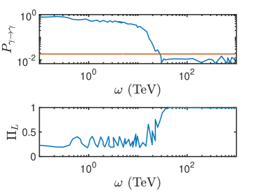
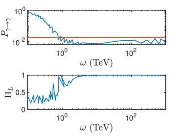
Figure 4: The photon survival probability $P_{\gamma\to\gamma}$ (upper) and the photon degree of polarization $\Pi_{L}$ (lower) as a function of the photon energy. Blue lines are results adopted from Figure 11 of Ref. Galanti:2022yxn , where photons originate from clusters at $z=0.03$ (left column) and at $z=0.4$ (right column). The red lines indicate $P_{\gamma\to\gamma}=1.8\%$.

In Fig. (4), we further compare the theoretical upper bound on the photon survival probability in the $z\geq z_{0}$ region, which is $P_{\gamma\to\gamma}<1.8\%$, to the actual calculations where different medium effects and varying magnetic fields are taken into consideration. We find that in the energy range where the photon polarization $\Pi_{L}\approx 1$, which is $\omega\gtrsim 20$ TeV ($\omega\gtrsim 1$ TeV) on the left (right) panel figure of Fig. (4), the photon survival probability is indeed below $1.8\%$.

5 Propagation modes for photons with energy $\omega=10^{-3}-10^{4}$ GeV

In this section, we discuss the propagation modes for photons with with energy $\omega=10^{-3}-10^{4}$ GeV. In this energy range, as compared to the ALP-photon mixing term, the quantity $\Gamma$ can also be considered negligible, in addition to the $\Delta_{x}$ and $\Delta_{y}$ terms, which are considered to be negligible in section 3. Thus our analytical analysis carried out in section 3 is still valid and can be further simplified by taking the $\Gamma\to 0$ limit. In section 3 we have neglected the ALP mass term. In this section we also study the effects of the ALP mass term.

We first discuss the case where the ALP mass term is neglected. In this case, we take the $\Gamma\to 0$ limit in Eqs. (16) and (17), which lead to

$$\rho_{x}(z)=\frac{1}{2},$$ (29)

$$\rho_{y}(z)=\frac{1}{2}\cos^{2}\left(\frac{g_{a\gamma}Bz}{2}\right).$$ (30)

Thus, both $\rho_{x}(z)$ and $\rho_{y}(z)$ are independent on energy, which also result in energy-independence of the photon survival probability $P_{\gamma\to\gamma}$ and the photon degree of polarization $\Pi_{L}$.

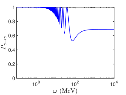
Figure 5: Photon survival probability as a function of the energy. Here we take the magnetic field as $B=5\ \mu\text{G}$, the coupling constant as $g_{a\gamma}=3\times 10^{-12}$ GeV, the propagation distance as $z=1\ \text{Mpc}$, and the ALP mass as $m_{a}=10^{-10}\ \text{eV}$.

We next discuss the case where the ALP mass term is important. We consider the case where $m_{a}=10^{-10}\ \text{eV}$. In this case, we have $\rho_{x}(z)=1/2$. The analytical form of $\rho_{y}(z)$ can be obtained by replacing $\Gamma$ in Eq. (17) with $i\Delta_{aa}=-im_{a}^{2}/(2\omega)$. Thus, we have

$$\rho_{y}(z)=\frac{1}{2}\left|\cos\left(\frac{\Delta}{2}z\right)+i\frac{\Delta_{aa}}{\Delta}\sin\left(\frac{\Delta}{2}z\right)\right|^{2},$$ (31)

where $\Delta=\sqrt{g_{a\gamma}^{2}B^{2}+m_{a}^{4}/(4\omega^{2})}$. We further compute the photon survival probability $P_{\gamma\to\gamma}$ and the polarization degree $\Pi_{L}$ by $P_{\gamma\to\gamma}=1/2+\rho_{y}$ and

$$\Pi_{L}=\frac{1-2\rho_{y}}{1+2\rho_{y}}=(P_{\gamma\to\gamma})^{-1}-1.$$ (32)

Thus, the polarization degree is solely determined by the photon survival probability $P_{\gamma\to\gamma}$.

Fig. (5) shows the relation between the photon survival probability $P_{\gamma\to\gamma}$ and the photon energy $\omega$. Interestingly, we find that there exist two energy regions where the photon survival probability $P_{\gamma\to\gamma}$ is (nearly) independent of the photon energy: (1) $\omega\lesssim 1$ MeV, (2) $\omega\gtrsim 300$ MeV. This can be understood as follows. If the photon energy $\omega$ is high such that the term $\Delta_{aa}=-m_{a}^{2}/(2\omega)$ can be neglected, this is just the case where the ALP mass can be neglected. Thus one should have energy-independent $\rho_{x}$ and $\rho_{y}$, as given in Eqs. (29) and (30), resulting in energy-independence in $P_{\gamma\to\gamma}$ for $\omega\gtrsim 300$ MeV in Fig. (5). If the photon energy is low such that $\Delta_{aa}/\Delta\to 1$, we have $\rho_{y}\to 1/2$. This then leads to $P_{\gamma\to\gamma}\approx 1$ for $\omega\lesssim 1$ MeV in Fig. (5).

The measurement of photon polarization degree can be carried out in the energy range of $10^{-1}-10^{4}\ \text{MeV}$ through advanced gamma-ray detectors, such as COSI COSI , e-ASTROGAM Kawata:2017zyo ; e-ASTROGAM:2018jlu , and AMEGO Kierans:2020otl , in the upcoming future. We note that the polarization degree, $\Pi_{L}$, can be indirectly determined using the relation $\Pi_{L}=(1/P_{\gamma\to\gamma}-1)$. Additionally, due to the photon-ALP interaction, the photon energy spectrum can exhibit a distinct oscillatory pattern sandwiched between two almost energy-independent regions, as illustrated in Fig. (5), which may serve as a novel signature for the ALP detection.

6 Conclusions

In this paper we have identified two distinct photon propagation modes in the presence of ALPs. We classify the two different modes by the sign of $D=(g_{a\gamma}B)^{2}-\Gamma^{2}$. For the $D>0$ propagation mode, the intensity of photon oscillates as propagating, producing multiple peaks along its propagation path. For the $D<0$ case, on the contrary, the intensity of photon does not exhibit any oscillatory behavior.

We use analytic methods to study the two photon propagation modes, because they are not readily discernible in numerical simulations, which have been extensively used in the literature to model the photon-ALP propagation. In our analytic methods, we assume a uniform magnetic field and negligible medium effects so that the propagation equation of the photon-ALP system can be solved in a simple analytic form.

We investigate photon propagation in two energy regions where our analytic methods are appropriate: (1) photon with energy $\gtrsim 100$ TeV; (2) photon in the energy range of $10^{-3}-10^{4}$ GeV. We identify the two photon propagation modes by comparing the magnetic field and the photon attenuation rate $\Gamma$ in different astrophysical environments. For the two propagation modes, We compute the photon survival probability $P_{\gamma\to\gamma}$ and the degree of photon polarization $\Pi_{L}$.

In the $D>0$ propagation mode of photons with energy $\gtrsim 100$ TeV, the fully-polarization can occur either in the $\rho_{x}\ll\rho_{y}$ case or in the $\rho_{y}\ll\rho_{y}$ case. Because of the oscillatory behavior in the intensity, the fully-polarization exhibits as various peaks in the propagation distance. In the $D<0$ propagation mode of photons with energy $\gtrsim 100$ TeV, there is no oscillation in the photon intensity. The detection condition that yields optimal results should include both a a nearly full-polarization signal and a considerable photon survival probability. The distances at which this condition is met in the $D<0$ case are $z\simeq z_{0}$ and $z\simeq 2z_{0}$, where $z_{0}$ is defined in Eq. (28). We further find an upper bound on the photon survival probability, $\simeq 1.8$ %, for the full-polarization region, $\Pi_{L}\approx 1$.

In the energy interval of $10^{-3}<\omega<10^{4}$ GeV, both medium and attenuation effects can become small compared to the ALP-photon mixing term, leading to even simpler analytic results. In this energy range, the propagation mode is predominately the $D>0$ mode in most of the parameter space of interest. We further find some distinguishing signatures associated with the ALP mass $m_{a}$: If $m_{a}\simeq 0$, both $P_{\gamma\to\gamma}$ and $\Pi_{L}$ are energy-independent; If $m_{a}$ cannot be neglected, there exist two energy-independent regions separated by an oscilating pattern in the energy spectrum of $P_{\gamma\to\gamma}$ and $\Pi_{L}$, which may serve as a novel signature to detect ALPs in the future experiments.

7 Acknowledgements

The work is supported in part by the National Natural Science Foundation of China under Grant Nos. 11675002, 11725520, 12147103, 12235001, and 12275128.

Appendix A Comparison between analytic and numerical calculations

In this section we compare analytic calculations based on a uniform magnetic field assumption, with the numerical calculations using a more realistic consideration of the magnetic field, both in the MW galaxy and in galaxy clusters.

A.1 MW galaxy

We first discuss the photon propagation in the MW galaxy. We adopt the MW magnetic field model given in Refs. Jansson:2012pc ; Jansson:2012rt , in which the magnetic field consists of two components: the regular component and the random component. Following Ref. Bi:2020ths , we neglect the random fields in our analysis. For completeness, we present the regular component of the MW magnetic field from Refs. Jansson:2012pc ; Jansson:2012rt in Table 1.

$i$	0	1	2	3	4	5	6	7
$r_{xi}$ (kpc)	5.1	6.3	7.1	8.3	9.8	11.4	12.7	15.5
$b_{i}$ ($\mu$G)		0.1	3.0	-0.9	-0.8	-2.0	-4.2	0

Table 1: The regular component of the magnetic field model in the MW disk Jansson:2012pc . The disk is partitioned into 7 regions with 8 boundaries that are given by $r_{i}=r_{xi}\exp(\phi\tan(90^{\circ}-\beta))$, where $\beta=11.5^{\circ}$; the $i$-th region is bounded by the two curves $r_{i-1}$ and $r_{i}$. The coordinates $(r,\phi)$ are defined such that the Galactic center is (0,0) and the Sun is (-8.5 kpc, 0). The direction of the regular component is $\hat{b}=\sin(\beta)\hat{r}+\cos(\beta)\hat{\phi}$; the magnitude of the regular component in the $i$-th region is given by $B=b_{i}{r_{0}}/{r}$ where $r_{0}=5$ kpc.

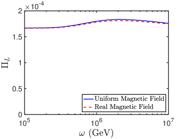
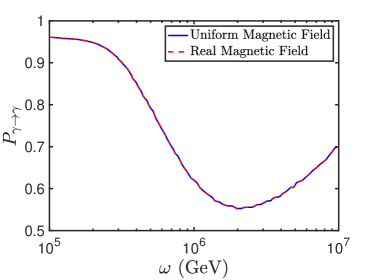
Figure 6: The polarization degree (left) and survival probability (right) as a function of the photon energy in the MW galaxy. The blue lines are obtained in analytic calculations where the medium effects are neglected and the magnetic field $B_{0}=0.98\ \mu$G is used. The red lines are obtained in numerical calculations where the medium effects ($\Delta_{x}$ and $\Delta_{y}$) and the MW magnetic field model are used (see main text).

We consider a source in the direction of $(\ell,b)=(180^{\circ},0^{\circ})$ (the opposite direction of GC) and with a distance of 4 kpc from Earth. In our analytic calculation we use $B_{0}=0.98\ \mu$G, which is the average value of the magnitude of the magnetic field along the propagation path. Fig. (6) shows the the polarization degree and survival probability, computed both in the analytic calculations and in the numerical calculations where the medium effects and the MW magnetic field model are used. The agreements between the analytic and numerical calculations indicate that the analytic calculation with a uniform magnetic field is a good approximation.

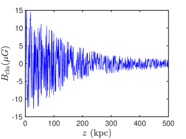
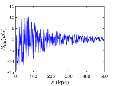
Figure 7: Simulated magnetic fields in the $x$- (left) and $y$- (right) directions in the galaxy cluster as a function of propagation distance $z$.

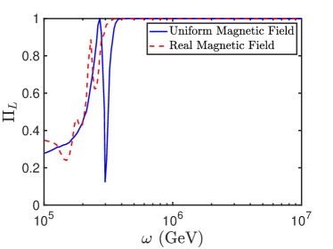
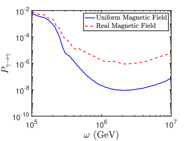
Figure 8: The polarization degree (left) and survival probability (right) as a function of the photon energy in the a galaxy cluster. The blue lines are obtained in analytic calculations where the medium effects are neglected and a uniform magnetic field of $B_{0}=0.19\ \mu$G is used. The red lines are obtained in numerical calculations where the medium effects are considered and the magnetic fields shown in Fig. 7 are used.

A.2 Galaxy clusters

We next discuss galaxy clusters. To model the complex magnetic field in galaxy clusters, we use the parametrization given in Refs. Galanti:2022yxn ; Bonafede:2010xg

$$B_{\rm clu}(z)=B_{\rm clu0}\left(1+\frac{z^{2}}{r_{\rm core}^{2}}\right)^{-\frac{3}{2}\eta\beta}.$$ (33)

For galaxy clusters, we adopt the following parameters: $B_{\rm clu0}=15$ $\mu$G, $r_{\rm core}=100$ kpc, $\beta=2/3$, and $\eta=0.75$ Galanti:2022yxn . Following Ref. Bonafede:2010xg , we assume that the direction of the magnetic field is random; hence, we simulate the magnetic field direction by using Monte Carlo method with a step of 1 kpc along the propagation path. Fig. (7) shows the simulated magnetic fields in the $x$- (left) and $y$- (right) directions in the galaxy cluster as a function of propagation distance $z$.

We obtain the mean value of the magnetic field in the galaxy cluster by taking the average of the magnetic field along the propagation path. In our simulation, we obtain $B_{0}=0.19\ \mu$G, which is the average of the magnetic field from $z=0$ to $z=500$ kpc. Fig. (8) shows the the polarization degree and survival probability, computed both in the analytic calculations and in the numerical calculations where the medium effects are considered and the magnetic field model given in Eq. (33) is used. We note that although the analytic calculation deviates from the numerical calculation, it describes the behavior qualitatively and provide valuable insights for ALP effects.

References

- (1) A. Ringwald, “Exploring the Role of Axions and Other WISPs in the Dark Universe,” Phys. Dark Univ. 1 (2012) 116–135 [arXiv:1210.5081].
- (2) I. G. Irastorza and J. Redondo, “New experimental approaches in the search for axion-like particles,” Prog. Part. Nucl. Phys. 102 (2018) 89–159 [arXiv:1801.08127].
- (3) C. B. Adams et al. in Snowmass 2021. 2022. arXiv:2203.14923.
- (4) R. D. Peccei and H. R. Quinn, “CP Conservation in the Presence of Instantons,” Phys. Rev. Lett. 38 (1977) 1440–1443.
- (5) F. Wilczek, “Problem of Strong and Invariance in the Presence of Instantons,” Phys. Rev. Lett. 40 (1978) 279–282.
- (6) J. Jaeckel and A. Ringwald, “The Low-Energy Frontier of Particle Physics,” Ann. Rev. Nucl. Part. Sci. 60 (2010) 405–437 [arXiv:1002.0329].
- (7) S. Chang, S. Tazawa, and M. Yamaguchi, “Axion model in extra dimensions with TeV scale gravity,” Phys. Rev. D 61 (2000) 084005 [hep-ph/9908515].
- (8) N. Turok, “Almost Goldstone bosons from extra dimensional gauge theories,” Phys. Rev. Lett. 76 (1996) 1015–1018 [hep-ph/9511238].
- (9) P. Svrcek and E. Witten, “Axions In String Theory,” JHEP 06 (2006) 051 [hep-th/0605206].
- (10) A. Ringwald in 4th Patras Workshop on Axions, WIMPs and WISPs, pp. 17–20. 2008. arXiv:0810.3106.
- (11) A. Arvanitaki, S. Dimopoulos, S. Dubovsky, N. Kaloper, and J. March-Russell, “String Axiverse,” Phys. Rev. D 81 (2010) 123530 [arXiv:0905.4720].
- (12) L. Maiani, R. Petronzio, and E. Zavattini, “Effects of Nearly Massless, Spin Zero Particles on Light Propagation in a Magnetic Field,” Phys. Lett. B 175 (1986) 359–363.
- (13) G. Raffelt and L. Stodolsky, “Mixing of the Photon with Low Mass Particles,” Phys. Rev. D 37 (1988) 1237.
- (14) H.-J. Li, J.-G. Guo, X.-J. Bi, S.-J. Lin, and P.-F. Yin, “Limits on axion-like particles from Mrk 421 with 4.5-year period observations by ARGO-YBJ and Fermi-LAT,” Phys. Rev. D 103 (2021) 083003 [arXiv:2008.09464].
- (15) D. Horns, L. Maccione, A. Mirizzi, and M. Roncadelli, “Probing axion-like particles with the ultraviolet photon polarization from active galactic nuclei in radio galaxies,” Phys. Rev. D 85 (2012) 085021 [arXiv:1203.2184].
- (16) R. Gill and J. S. Heyl, “Constraining the photon-axion coupling constant with magnetic white dwarfs,” Phys. Rev. D 84 (2011) 085001 [arXiv:1105.2083].
- (17) X.-J. Bi, et al., “Axion and dark photon limits from Crab Nebula high energy gamma-rays,” Phys. Rev. D 103 (2021) 043018 [arXiv:2002.01796].
- (18) G. Galanti, “Photon-ALP oscillations inducing modifications to photon polarization,” Phys. Rev. D 107 (2023) 043006 [arXiv:2202.11675].
- (19) G. Galanti, M. Roncadelli, F. Tavecchio, and E. Costa, “ALP induced polarization effects on photons from galaxy clusters,” Phys. Rev. D 107 (2023) 103007 [arXiv:2202.12286].
- (20) Z.-Q. Xia, et al., “Searching for the possible signal of the photon-axionlike particle oscillation in the combined GeV and TeV spectra of supernova remnants,” Phys. Rev. D 100 (2019) 123004 [arXiv:1911.08096].
- (21) Y.-F. Liang, et al., “Constraints on axion-like particle properties with TeV gamma-ray observations of Galactic sources,” JCAP 06 (2019) 042 [arXiv:1804.07186].
- (22) A. De Angelis, G. Galanti, and M. Roncadelli, “Relevance of axion-like particles for very-high-energy astrophysics,” Phys. Rev. D 84 (2011) 105030 [arXiv:1106.1132]. [Erratum: Phys.Rev.D 87, 109903 (2013)].
- (23) S. Vernetto and P. Lipari, “Absorption of very high energy gamma rays in the Milky Way,” Phys. Rev. D 94 (2016) 063009 [arXiv:1608.01587].
- (24) P. Lipari and S. Vernetto, “Diffuse Galactic gamma ray flux at very high energy,” Phys. Rev. D 98 (2018) 043003 [arXiv:1804.10116].
- (25) W. Dittrich and H. Gies, Probing the quantum vacuum. Perturbative effective action approach in quantum electrodynamics and its application, vol. 166. 2000.
- (26) J. I. Latorre, P. Pascual, and R. Tarrach, “Speed of light in nontrivial vacua,” Nucl. Phys. B 437 (1995) 60–82 [hep-th/9408016].
- (27) M. V. Cougo-Pinto, C. Farina, F. C. Santos, and A. Tort, “The speed of light in confined QED vacuum: Faster or slower than c?” Phys. Lett. B 446 (1999) 170–174.
- (28) R. Tarrach, “Thermal Effects on the Speed of Light,” Phys. Lett. B 133 (1983) 259–261.
- (29) S. L. Adler, “Photon splitting and photon dispersion in a strong magnetic field,” Annals Phys. 67 (1971) 599–647.
- (30) A. Dobrynina, A. Kartavtsev, and G. Raffelt, “Photon-photon dispersion of TeV gamma rays and its role for photon-ALP conversion,” Phys. Rev. D 91 (2015) 083003 [arXiv:1412.4777]. [Erratum: Phys.Rev.D 95, 109905 (2017)].
- (31) A. Kosowsky, “Introduction to microwave background polarization,” New Astron. Rev. 43 (1999) 157 [astro-ph/9904102].
- (32) G. B. Rybicki and A. P. Lightman, Radiative Processes in Astrophysics. 1979.
- (33) J. M. Yao, R. N. Manchester, and N. Wang, “A new electron density model for estimation of pulsar and FRB distances,” The Astrophysical Journal 835 (2017) 29.
- (34) A. Kartavtsev, G. Raffelt, and H. Vogel, “Extragalactic photon-ALP conversion at CTA energies,” JCAP 01 (2017) 024 [arXiv:1611.04526].
- (35) G. Galanti and M. Roncadelli, “Axion-like Particles Implications for High-Energy Astrophysics,” Universe 8 (2022) 253 [arXiv:2205.00940].
- (36) A. Mirizzi and D. Montanino, “Stochastic conversions of TeV photons into axion-like particles in extragalactic magnetic fields,” JCAP 12 (2009) 004 [arXiv:0911.0015].
- (37) I. G. Irastorza, “An introduction to axions and their detection,” SciPost Phys. Lect. Notes 45 (2022) 1 [arXiv:2109.07376].
- (38) R. Jansson and G. R. Farrar, “A New Model of the Galactic Magnetic Field,” Astrophys. J. 757 (2012) 14 [arXiv:1204.3662].
- (39) R. Jansson and G. R. Farrar, “The Galactic Magnetic Field,” Astrophys. J. Lett. 761 (2012) L11 [arXiv:1210.7820].
- (40) R. E. Pudritz, M. J. Hardcastle, and D. C. Gabuzda, “Magnetic Fields in Astrophysical Jets: From Launch to Termination,” Space Sci. Rev. 169 (2012) 27–72 [arXiv:1205.2073].
- (41) F. Tavecchio, G. Ghisellini, G. Ghirlanda, L. Foschini, and L. Maraschi, “TeV BL Lac objects at the dawn of the Fermi era,” Mon. Not. Roy. Astron. Soc. 401 (2010) 1570 [arXiv:0909.0651].
- (42) F. Govoni and L. Feretti, “Magnetic field in clusters of galaxies,” Int. J. Mod. Phys. D 13 (2004) 1549–1594 [astro-ph/0410182].
- (43) A. Neronov and I. Vovk, “Evidence for strong extragalactic magnetic fields from Fermi observations of TeV blazars,” Science 328 (2010) 73–75 [arXiv:1006.3504].
- (44) M. S. Pshirkov, P. G. Tinyakov, and F. R. Urban, “New limits on extragalactic magnetic fields from rotation measures,” Phys. Rev. Lett. 116 (2016) 191302 [arXiv:1504.06546].
- (45) C. Y. Yang, et al. in Space Telescopes and Instrumentation 2018: Ultraviolet to Gamma Ray, J.-W. A. den Herder, S. Nikzad, and K. Nakazawa, eds., vol. 10699 of Society of Photo-Optical Instrumentation Engineers (SPIE) Conference Series, p. 106992K. 2018.
- (46) K. Kawata, et al., “Energy determination of gamma-ray induced air showers observed by an extensive air shower array,” Exper. Astron. 44 (2017) 1–9.
- (47) G. Z. Angeli and P. Dierickx, eds., “The e-ASTROGAM gamma-ray space observatory for the multimessenger astronomy of the 2030s,” Proc. SPIE Int. Soc. Opt. Eng. 10699 (2018) 106992J [arXiv:1805.06435].
- (48) AMEGO Team Collaboration, “AMEGO: Exploring the Extreme Multimessenger Universe,” Proc. SPIE Int. Soc. Opt. Eng. 11444 (2020) 1144431 [arXiv:2101.03105].
- (49) A. Bonafede, et al., “The Coma cluster magnetic field from Faraday rotation measures,” Astron. Astrophys. 513 (2010) A30 [arXiv:1002.0594].