Evolutionary Monte Carlo of QM properties in chemical space: Electrolyte design

Abstract

Optimizing a target function over the space of organic molecules is an important problem appearing in many fields of applied science, but also a very difficult one due to the vast number of possible molecular systems. We propose an Evolutionary Monte Carlo algorithm for solving such problems which is capable of straightforwardly tuning both exploration and exploitation characteristics of an optimization procedure while retaining favourable properties of genetic algorithms. The method, dubbed MOSAiCS (Metropolis Optimization by Sampling Adaptively in Chemical Space), is tested on problems related to optimizing components of battery electrolytes, namely minimizing solvation energy in water or maximizing dipole moment while enforcing a lower bound on the HOMO-LUMO gap; optimization was done over sets of molecular graphs inspired by QM9 and Electrolyte Genome Project (EGP) datasets. MOSAiCS reliably generated molecular candidates with good target quantity values, which were in most cases better than the ones found in QM9 or EGP. While the optimization results presented in this work sometimes required up to $10^{6}$ QM calculations and were thus only feasible thanks to computationally efficient ab initio approximations of properties of interest, we discuss possible strategies for accelerating MOSAiCS using machine learning approaches.

1 Introduction

Increasing efficiency and longevity of energy storage systems is critical for improving economic sustainability of lowering greenhouse gas emissions.¹ One aspect of this problem is searching chemical compound space for organic molecules optimal for a target application, such as lithium battery electrolyte component^{2, 3, 4, 5, 6} or electroactive molecules for redox flow batteries.^{7, 8} In this work we focused on the former, more specifically on finding electrochemically stable organic molecules that are good solvents for alkali salts. While such searches can be aided with high-throughput screening,^{2, 3, 4} there has been a surge of ways to go beyond by increasing efficiency of compound property evaluations, e.g. with machine learning⁹ or quantum alchemy,^{10, 11, 12} and by sampling chemical space more efficiently. In the context of optimizing small organic molecules, most methods of the latter category can be classified as those based on Markov decision processes,^{13, 14, 15, 16, 17, 18} recurrent neural networks,^{19, 20} genetic algorithms,^{21, 22, 23, 24, 25, 26} and variational autoencoders.^{27, 28}

While several variants of Markov chain Monte Carlo²⁹ sampling have also been applied to molecule optimization problems,^{30, 31} one intriguing variant, namely Evolutionary Monte Carlo,^{32, 33, 34} has been overlooked so far. The approach combines two philosophies that have demonstrated reliable performance for a range of optimization problems: parallel tempering^{35, 36, 37} and genetic algorithms.^{38, 39, 40} As illustrated in Figure 1, Evolutionary Monte Carlo involves running several Markov chain Monte Carlo simulations that focus on exploitation (i.e. refining already known molecules via incremental changes) or exploration (i.e. finding promising regions of chemical space), which interact by swapping configurations analogously to parallel tempering or by creating “child configurations” similarly to genetic algorithms in a way that observes detailed balance condition.⁴¹ As is the case for genetic algorithms, increasing the number of replicas yields more opportunities for creating ”child configurations,” thus accelerating exploration of chemical space. Unlike genetic algorithms though, Evolutionary Monte Carlo allows straightforward control of its exploration and exploitation aspects while guaranteeing to eventually find the global minimum due to the properties of Markov chain Monte Carlo. Evolutionary Monte Carlo can also potentially be combined with nested Monte Carlo techniques^{42, 43, 44} to utilize multiple optimized quantity evaluation methods at once, e.g. when laboratory experiments are used alongside theoretical and machine learning approaches,^{45, 46, 47, 48} an advantage particularly relevant for high-throughput automated laboratory workflows.^{49, 50, 51, 48}

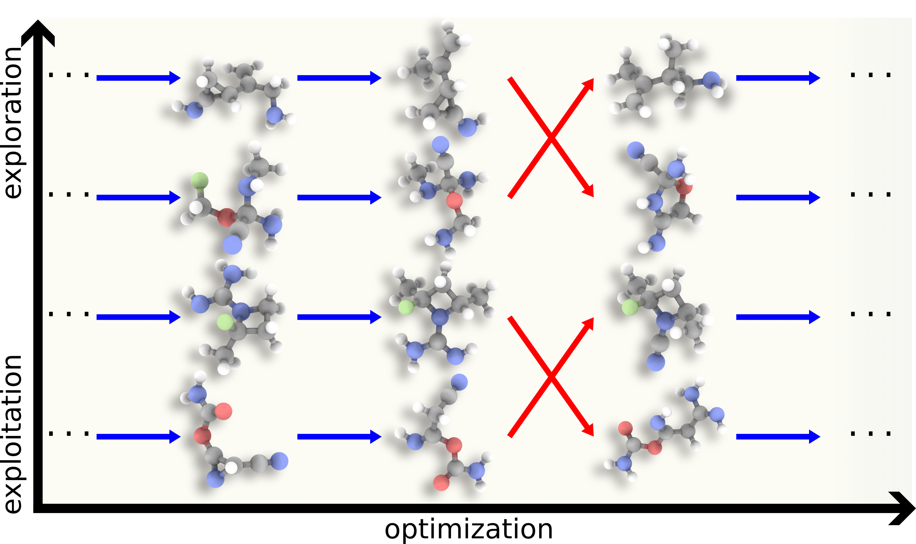
Figure 1: Scheme of an Evolutionary Monte Carlo workflow for molecular optimization that introduces several replicas with varying degree of focus on exploitation or exploration aspects of the calculation and evolves them by applying elementary mutations (blue) to single replicas and crossover moves (red) to pairs of replicas in a way satisfying detailed balance.

With these reasons in mind, we implemented an Evolutionary Monte Carlo algorithm inspired by a family of genetic algorithms for optimization in the space of molecular graphs.^{21, 22, 23, 24} While some recently proposed methods for molecular optimization operate in string representations,^{19, 18, 52, 25, 53} we performed all procedures directly on chemical graphs to facilitate ensuring validity of generated molecules and maintaining detailed balance, as well as provide a more direct connection between the molecules considered and graph-based representations that have proven efficient in machine learning applications.^{54, 55} Lastly, we implemented a simple Wang-Landau biasing potential⁵⁶ as a curiosity reward⁵⁷ increasing exploration aspect of the algorithm by “pushing” our Markov chain Monte Carlo simulations out of previously occupied graphs. The resulting method is named MOSAiCS (Metropolis Optimization by Sampling Adaptively in Chemical Space). While we were mainly designing our approach with battery applications in mind, we think it should be useful for other molecular optimization problems, such as those arising in drug design.^{19, 58, 15, 31, 17, 59, 60}

The rest of the paper is organized as follows. Section 2 presents the main ideas behind our approach in Subsecs. 2.1-2.3, following up with description of the optimization problem on which we test it in Subsec. 2.4 and details of our Monte Carlo simulations in Subsec. 2.5. Section 3 discusses our experimental results, Section 4 concludes the paper with a results summary and outline of possible strategies to improve our approach. Some technical details of our method’s implementation, experimental setup, and results were left for Supporting Information.

2 Theory

2.1 Chemical space definition

We aim to minimize a loss function $F$ over a set of molecules, the latter represented by their chemical graphs. We define a chemical graph as an undirected graph whose nodes correspond to heavy atoms, along with, where present, hydrogen atoms covalently connected to them, and whose edges connect a pair of nodes if their heavy atoms share a covalent bond. For a chemical graph we also define a resonance structure as a set of valences of nodes’ heavy atoms and orders of covalent bonds connecting these heavy atoms, both quantities taking integer values. The sum of covalent bond orders connecting a heavy atom to other atoms equals its valence, with the orders of bonds between a heavy atom and a hydrogen atom counted as one. Valence numbers are chosen to be chemically reasonable (e.g. IV for C, II, or IV, or VI for S) and we require their sum to be the minimum needed to build a set of covalent bond orders. We also forbid a covalent bond order to be larger than three. The reasons for not including valences and bond orders in the definition of a chemical graph, but rather enumerating their possible values separately, are illustrated in Figure 2 demonstrating examples of molecules for which several resonance structures differing in bond orders or bond orders and heavy atom valences can be defined. We emphasize that while this definition of bond orders and valences is loosely based on valence structure theory, it was designed not to reflect actual electronic structure of a molecule, but to allow convenient definitions of changes of chemical graphs that are illustrated in Figures 3 and 4, as will be discussed in detail in Subsec. 2.3.

Our definition of chemical graph a priori prevents us from differentiating between conformers or stereoisomers and we will assume our optimization problem to be unaffected by this, e.g. if for a given chemical graph we are interested only in the most stable stereoisomer and we optimize a Boltzmann average. We also did not implement support for molecules where valid Lewis structures can only be generated by assigning charges to atoms, e.g. compounds with nitro groups, hence they were ignored during all calculations done in this work.

Figure 2: Examples of molecules that can be written in terms of several resonance structures that differ in (a) covalent bond orders and (b) both covalent bond orders and heavy atom valences.

2.2 Monte Carlo sampling

We perform optimization by running a Markov chain Monte Carlo simulation (referred to as just “simulation” from now on) of unnormalized probability density similar to the one used for parallel tempering

$$\begin{split}P(\mathbf{X})=&\exp\left\{-\sum_{i=1}^{N_{\mathrm{opt}}}C^{\infty}\left[F\left(X^{(i)}\right)\right]\right.\\ &\left.-\sum_{i=N_{\mathrm{opt}}+1}^{N_{\mathrm{repl}}}\beta^{(i)}\left[F\left(X^{(i)}\right)+V_{\mathrm{bias}}^{(i)}\left(X^{(i)}\right)\right]\right\},\end{split}$$ (1)

where $\mathbf{X}$ is a set of $N_{\mathrm{repl}}$ chemical graphs (also referred to as replicas) $X^{(i)}$ ($i=1,\ldots,N_{\mathrm{repl}}$), $\beta^{(i)}$ ($i=N_{\mathrm{opt}}+1,\ldots,N_{\mathrm{repl}}$) are temperature parameters, $V_{\mathrm{bias}}$ is biasing potential, $C^{\infty}$ is the “infinitely convex function” defined to be such that for arbitrary sets of numbers $x^{(j)}$ and $y^{(j)}$ ($j=1,\ldots,N_{\mathrm{opt}}$)

$$\begin{split}\min_{j=1,\ldots,N_{\mathrm{opt}}}x^{(j)}-\min_{j=1,\ldots,N_{\mathrm{opt}}}y^{(j)}<0\Leftrightarrow\\ \sum_{j=1}^{N_{\mathrm{opt}}}\left[C^{\infty}(x^{(j)})-C^{\infty}(y^{(j)})\right]\rightarrow+\infty,\end{split}$$ (2)

and $N_{\mathrm{opt}}$ is the number of replicas that, as will become clear later, effectively undergo greedy stochastic minimization and are referred to as greedy replicas, with the other replicas, referred to as exploration replicas, providing a less restricted exploration of chemical space and preventing greedy replicas from getting stuck in a local minimum of $F$. The history-dependent biasing potential $V_{\mathrm{bias}}^{(i)}$ is defined as⁵⁶

$$V_{\mathrm{bias}}^{(i)}\left(X\right)=\frac{\alpha_{b}}{\beta^{(i)}}\sum_{j=N_{\mathrm{opt}}+1}^{N_{\mathrm{repl}}}\rho^{(j)}(X),$$ (3)

where $\rho^{(j)}(X)$ is the number of times $X$ has been visited during the simulation by replica with index $j$ (details on how it was evaluated are left for Subsec. 2.5), $\alpha_{b}$ is the user-defined bias proportionality coefficient. Setting a non-zero $\alpha_{b}$ makes sampling $\mathbf{X}$ non-Markovian; as a result our certainty that in this regime a global minimum of $F$ w.r.t. $X$ is eventually found is based not on properties of Markov chain Monte Carlo, but on heuristic expectation that the biasing potential would make probability distribution of each exploration replica approach uniformity, leading to at least one replica coming across the global minimum over a finite number of simulation steps.

2.3 Monte Carlo moves

A simulation consists of taking a sequence of moves in a way outlined in Algorithm 1. If the current set of replicas is in configuration $\mathbf{X}_{1}$, a move involves randomly generating parameters $\mathbf{w}$ of a change and deciding to replace $\mathbf{X}_{1}$ with the change’s outcome (or trial configuration) $\mathbf{X}_{2}$ with an acceptance probability similar to the standard Metropolis-Hastings expression⁴¹

$$\begin{split}P_{\mathrm{acc}}\left(\mathbf{X}_{1},\mathbf{w},\mathbf{X}_{2}\right)=&\mathrm{min}\left[1,\vphantom{\frac{P_{\mathrm{prop}}\left(\mathbf{X}_{\mathrm{2}},\mathbf{w}^{-1}\right)P\left(\mathbf{X}_{2}\right)}{P_{\mathrm{prop}}(\mathbf{X}_{1},\mathbf{w})P\left(\mathbf{X}_{1}\right)}}\right.\\ &\left.\frac{P_{\mathrm{prop}}(\mathbf{X}_{1},\mathbf{w})P\left(\mathbf{X}_{2}\right)}{P_{\mathrm{prop}}\left(\mathbf{X}_{\mathrm{2}},\mathbf{w}^{-1}\right)P\left(\mathbf{X}_{1}\right)}\right],\end{split}$$ (4)

where $P_{\mathrm{prop}}(\mathbf{X}_{1},\mathbf{w})$ is the probability that $\mathbf{w}$ is proposed given that $\mathbf{X}_{1}$ is the initial configuration and $\mathbf{w}^{-1}$ are parameters of a random change yielding $\mathbf{X}_{1}$ when applied to $\mathbf{X}_{2}$ and corresponding to a unique $\mathbf{w}$. The latter property ensures that detailed balance still holds in situations when several $\mathbf{w}$ yield the same trial configuration $\mathbf{X}_{2}$. Trial configurations decreasing the minimal value of $F$ among greedy replicas compared to initial configurations is accepted automatically due to our definition of $C^{\infty}$ (2).

Algorithm 1 Sampling $P(\mathbf{X})$ (1).

0:  Initial configuration: $\mathbf{X}_{1}$;

  loop

     Randomly choose change parameters $\mathbf{w}$;

     Use $\mathbf{w}$ on $\mathbf{X}_{1}$ to generate $\mathbf{X}_{2}$;

     Randomly sample $r$ from uniform distribution in $[0,1]$;

     $r_{\mathrm{acc.}}\leftarrow P_{\mathrm{acc.}}(\mathbf{X}_{1},\mathbf{w},\mathbf{X}_{2})$ (see Eq. (4);

     if $r<r_{\mathrm{acc.}}$ then

        $\mathbf{X}_{1}\leftarrow\mathbf{X}_{2}$;

     end if

  end loop

We use three types of moves to propose the trial configurations $\mathbf{X}_{2}$; we will only discuss the general idea behind them here with implementation details left for Supporting Information. The first type, referred to as elementary moves, applies an elementary mutation outlined in Figure 3 to a single replica; such moves correspond to incremental exploration of chemical space. To accelerate greedy optimization of molecules, we additionally introduced the “no reconsiderations condition”: if change parameters $\mathbf{w}$ corresponding to an elementary move have been rejected for a greedy replica they are not considered again. The second type of moves is tempering swap moves that are analogous to the swap moves in conventional parallel tempering techniques and involve randomly choosing replicas with indices $i$ and $j$ in such a way that at least one of them is an exploration replica, considering a swap of the corresponding chemical graphs, and accepting it with acceptance probability (4). These moves allow greedy replicas stuck in a local minimum of $F$ to get to chemical graphs with lower values of $F$ if the latter are discovered by an exploration replica.

M1: Addition/removal of a node (red) connected to a single neighbor (blue).	M2: Changing order of a covalent bond (green) and number of hydrogen atoms in the nodes it connects (blue).
M3: Replacing a heavy atom (red) in a node without changing its connections to other nodes.	M4: Change valence of a heavy atom (green) by adding or removing hydrogen atoms connected to it.
M5: Change valence of a heavy atom (green) by adding or removing nodes (red) connected to it.	M6: Change valence of a heavy atom (green) by changing order of a covalent bond (green) with another node whose hydrogen number is changed (blue).

Figure 3: Definitions and examples of elementary mutations. A node is colored green if its heavy atom changes valence, otherwise it is colored red if it is destroyed or created, or colored blue if it changes the number of hydrogen atoms connected to the heavy atom. A bond is colored red if it is destroyed or created or green if it, in general, only changes bond order, though the latter may involve changing the order to and from 0. The valences in M5 and M6 always change to adjacent values (e.g. for S valence can change from II to IV, but not from II to VI); nodes created and destroyed in M1, M3, and M5 contain heavy atoms in their smallest valence state (e.g. valence II for S).

The third type of moves are crossover moves inspired by the procedure developed in Ref. 21, which are introduced to allow drastic changes of chemical graphs occupied by replicas. The general idea is illustrated in Figure 4: a pair of nodes is randomly chosen in two chemical graphs and the neighborhoods of these two nodes are exchanged to create two new chemical graphs. Thus defined crossover moves are more restrictive than the ones of Ref. 21 as they do not allow exchanging fragments of arbitrary shape and connectivity. These restrictions, however, make it straightforward to ensure that the resulting chemical graphs satisfy constraints on the number of nodes, are connected, and correspond to a change for which the $P_{\mathrm{prop}}(\mathbf{X}_{1},\mathbf{w})/P_{\mathrm{prop}}(\mathbf{X}_{2},\mathbf{w}^{-1})$ ratio in $P_{\mathrm{acc}}$ (4) can be easily calculated.

Figure 4: An example of a crossover move. I - selection of two “blue” nodes in two molecules; II - selecting the “blue” neighborhoods of the two blue nodes, coloring the rest “red,” with the bonds connecting blue and red fragments colored “green”; III - exchanging the blue fragments between molecules and reconnecting them with red fragments by exchanging connected nodes between pairs of green bonds.

Setting $F$ to be infinitely large for chemical graphs violating certain user-defined constraints is a general way to enforce the latter on the optimization result. However, it is in general preferable to maintain a given constraint as early as during the proposition of trial configuration $\mathbf{X}_{2}$ to increase average acceptance probability and the resulting speed of chemical space exploration. We implemented the corresponding algorithms for maintaining constraints on the number of heavy atoms in a molecule and the kinds of atoms that can share a covalent bond since they are simple to maintain, yet quite important for our applications. Lastly, the question of the moves’ sufficiency to access the chemical space and sets of molecules considered in Section 3 in their entirety is discussed in Supporting Information.

2.4 Minimization problems

A good battery electrolyte is a good solvent for lithium salts and is electrochemically stable. We approximated the former property with polarity; maximizing a molecule’s polarity was in turn approximated by either maximizing the dipole moment $D$ or minimizing the free energy of solvation in water $\Delta G_{\mathrm{solv}}$. We approximated the electrochemical stability requirement with a lower bound on the HOMO-LUMO $\Delta\epsilon$, with which we approximated the width of the compound’s electrochemical stability window.² While the latter relation is not actually practical for battery design,⁶¹ we still opted for a $\Delta\epsilon$-based electrochemical stability criterion to connect our work with other compound optimization problems where $\Delta\epsilon$ can be used.^{62, 63} For both $D$ and $\Delta G_{\mathrm{solv}}$ optimization we constrained the molecules’ $\Delta\epsilon$ to be larger than either benzene (strong $\Delta\epsilon$ constraint) or octa-1,3,5,7-tetraene (weak $\Delta\epsilon$ constraint), resulting in four minimization problems of differing difficulty. While in this work we focused on testing performance of MOSAiCS against these single objective optimization problems, our approach can also be used to optimize several properties at once via a suitable multiobjective loss function.⁶⁴

We aimed to estimate $\Delta G_{\mathrm{solv}}$, $D$, and $\Delta\epsilon$ as computationally cheaply as possible while being qualitatively correct over a wide range of chemical compounds; the resulting protocol is explained in detail in Supporting Information. Here we just mention that for a given chemical graph we used the MMFF94 forcefield^{65, *Halgren:1996_II, *Halgren:1996_III, *Halgren_Nachbar:1996_IV, *Halgren:1996_V, *Halgren:1999_VI, *Halgren:1999_VII} to generate molecular conformers, for which we performed GFN2-xTB⁷² calculations with analytical linearized Poisson-Boltzmann model⁷³ simulating presence of water. The root mean square error (RMSE) that is presented for calculated quantities corresponds to statistical error from randomness of conformer generation. We used two sets of parameters for our protocol: “converged” that produced reasonable RMSEs for a wide variety of compounds, but was relatively computationally expensive, and “cheap” that was used during our simulations. From now on, $\Delta G_{\mathrm{solv}}$, $D$, and $\Delta\epsilon$ will denote estimates of these quantities obtained with the “converged” protocol, while estimates obtained with the “cheap” protocol will be marked with addition of “cheap” superscript.

Each of the four minimization problems was solved in two sets of molecules based on QM9^{74, *Ramakrishnan_Lilienfeld:2014} and the Electrolyte Genome Project⁵ (EGP) datasets. The QM9 dataset consists of 134k molecules containing up to 9 heavy atoms (C, O, N, and F). We defined the “QM9*” set to consist of molecules (not necessarily in QM9) that also contain up to 9 heavy atoms of the same elements as QM9, but are additionally constrained by not allowing bonds between N, O, and F atoms, as well as O-H and H-F bonds, since these covalent bonds are typically associated with increased chemical reactivity. The EGP dataset was generated with the Materials Project⁷⁶ workflows in an effort to facilitate discovery of novel battery electrolyte molecules; the version currently hosted on the Materials Project website contains 24.5k species in total; neutral species for which MMFF94 coordinates could be generated included 19.7k individual chemical graphs containing up to 92 heavy atoms. These characteristics of the EGP dataset were the basis for defining the “EGP*” set, whose molecules (not necessarily in EGP) contain up to 15 heavy atoms (B, C, N, O, F, Si, P, S, Cl, and Br, which are elements present in organic molecules of EGP) and, for the sake of chemical stability, do not contain covalent bonds between N, O, F, Cl, and Br, between H and B, O, F, Si, P, S, Cl, or Br, as well as S-S and P-P bonds.

We chose 15 as the maximum number of heavy atoms allowed in EGP* molecules because this size restriction is obeyed by 87.0% and 97.0% of EGP’s chemical graphs satisfying weak and strong $\Delta\epsilon$ constraints. When choosing which elements can not share a covalent bond in QM9* and EGP* molecules we mainly aimed for excluding weak bonds, although we also forbade some relatively strong bonds whose presence can signify molecular reactivity. Since we only consider molecules whose valid Lewis structures can be generated without assigning charges to atoms, H-F and double O-O bonds can only be encountered in hydrogen fluoride and oxygen, which we excluded from consideration due to their corrosive properties. Creating N-N bonds inside an organic compound risks making it prone to releasing nitrogen on excitation, adding functional groups containing double N-O bonds to a molecule risks making the latter prone to self-oxidation, and hydroxyl groups engage relatively easily in reactions involving oxidation or nucleophilic attacks.⁷⁷ We note that in practice, managing this kind of reactive behavior would require additional use of more sophisticated compound stability measures.

While both QM9* and EGP* are well defined and finite sets of chemical graphs, their huge size makes evaluating any of their properties exactly, i.e. through exact enumeration of all their chemical graphs, unfeasible. However, we do summarize properties of intersections of QM9* and QM9, as well as EGP* and EGP, in Supporting Information.

2.5 Simulation details

During a simulation we used $\Delta\epsilon^{\mathrm{cheap}}$ to estimate whether a molecule satisfies the constraint on $\Delta\epsilon$; dimensionless loss functions corresponding to $D$ and $\Delta G_{\mathrm{solv}}$ were defined as

$$F_{\mathrm{solv.}}(X)= \frac{\Delta G_{\mathrm{solv}}^{\mathrm{cheap}}(X)}{\mathrm{STD}_{\mathrm{dataset}}(\Delta G_{\mathrm{solv}})},$$ (5)

$$F_{\mathrm{dipole}}(X)= -\frac{D^{\mathrm{cheap}}(X)}{\mathrm{STD}_{\mathrm{dataset}}(D)},$$ (6)

where $\mathrm{STD}_{\mathrm{dataset}}$ refers to standard deviation of a quantity over molecules at the intersection of chemical graph set of interest and the reference dataset (QM9 for QM9* and EGP for EGP*) which satisfy the $\Delta\epsilon$ constraint of interest. We chose 1000 “pre-final” molecules exhibiting the smallest value of loss function out of the molecules visited during the simulation and evaluated converged estimates of the quantities of interest for them; the molecule with the best $D$ or $\Delta G_{\mathrm{solv}}$ value among pre-final molecules satisfying the $\Delta\epsilon$ constraint is the one considered the candidate molecule proposed by the simulation.

We used $N_{\mathrm{repl}}=36$ with $N_{\mathrm{opt}}=4$ (cf. definitions in Subsection 2.2); virtual temperature parameters $\beta^{(i)}$ appearing in $P$ (1) were defined in such a way that the smallest and largest $\beta^{(i)}$ were 1 and 8, and the other $\beta^{(i)}$ formed a geometric progression between the two extrema values, the latter being a simple recipe taken from applications of parallel tempering to configuration space sampling.^{78, 79} A simulation consisted of 50000 “global” steps, out of which 60% were “simple” steps applying an elementary move to each replica, 20% were “tempering” steps making tempering swap moves on 128 randomly chosen pairs of replicas, and another 20% were “crossover” steps making crossover moves on 32 randomly chosen pairs of replicas. $\rho^{(j)}(X)$ appearing in $V_{\mathrm{bias}}^{(i)}$ (3) was counted as the number of times replica $j$ was found in $X$ after a global step had been completed. For elementary moves we additionally set that: the nodes added or removed during M1 mutation could be connected to the molecule with bonds of order from 1 to 3; bonds changed with M2 and M6 mutations could have their order increased or decreased by 1 and 2 respectively; nodes added or removed with M5 mutation could be connected to the molecule with bonds of order 1 or 2.

We set $\alpha_{b}$ to $0.0$, $0.2$, or $0.4$; for each of the resulting 12 combinations of $\alpha_{b}$ and optimization problem we ran 8 simulations with different random number generator seeds. For all simulations all replicas initially occupied the chemical graph of methane. While it would be natural to assign each replica a randomly chosen molecule from the intersection of QM9 and QM9* or EGP and EGP*, we went with the intentional handicap of using methane as the starting molecule to demonstrate that MOSAiCS is capable of constructing all the candidate molecules presented in this Section from scratch. The effect of choice of initial conditions on the final result is briefly addressed in Supporting Information.

3 Results and discussion

In this Section we describe the main results of our numerical experiments. The more technical aspects, such as full information on generated candidates and influence of biasing potential on search efficiency, are left for Supporting Information.

While we ran in total 96 simulations in QM9*, or 24 simulations with different random generator seed and $\alpha_{b}$ values for each optimization problem, they agreed remarkably often on candidates proposed, only yielding 10 candidates in total. Table 1 summarizes the best and worst values of optimized quantities of candidates proposed by MOSAiCS along with the corresponding relative improvement, which we define as absolute difference between a candidate’s optimized quantity value and the corresponding value for the best molecule for the optimization problem taken from the reference dataset (cf. Table S2 in Supporting Information), divided by the corresponding $\mathrm{STD}_{\mathrm{dataset}}$. For optimization of $\Delta G_{\mathrm{solv}}$ with weak $\Delta\epsilon$ constraint all trajectories proposed the minimum of $\Delta G_{\mathrm{solv}}$ already present in QM9, while for all other optimization problems all trajectories proposed candidates that improved significantly on molecules in QM9. Best candidates proposed for a given optimization problem are shown in Figure 5; note that to facilitate discussion of candidates’ properties in Supporting Information, each candidate is referred by a capital $C$ with a unique index subscript and a superscript denoting the reference dataset. We see how MOSAiCS successfully constructed complex conjugated bond structures facilitating charge transfer which, in turn, led to smaller, i.e. more negative, $\Delta G_{\mathrm{solv}}$ or larger $D$. Figure 6 displays optimization progress with number of global Monte Carlo steps for different $\alpha_{b}$ values for minimizing $\Delta G_{\mathrm{solv}}$ with weak $\Delta\epsilon$ constraint. We observe convergence of the optimized property with a rate not significantly affected by changing $\alpha_{b}$; the same is true with varying degree for other optimization problems as discussed in Supporting Information. To visualize how simulations explored chemical space for different optimization problems and values of $\alpha_{b}$, for each such combination we took a simulation that had produced the best candidate and plotted the density of molecules it encountered with respect to the optimized quantity and $\Delta\epsilon$. Figure 7 presents such plots for minimizing $\Delta G_{\mathrm{solv}}$ with weak $\Delta\epsilon$ constraint, with plots for other optimization problems presented and discussed in Supporting Information. We see that increasing $\alpha_{b}$ tended to increase diversity of molecules encountered during the simulations, but this was mainly done by considering more molecules in regions of chemical space with larger values of $\Delta G_{\mathrm{solv}}$.

optimized	$\Delta\epsilon$	optimized quantity value			relative improvement
quantity	constraint	best	worst		best	worst
$\Delta G_{\mathrm{solv}}$	weak	$-94.79\pm 0.06\phantom{0}$	_		$0.004\pm 0.009$	_
	strong	$-68.19\pm 0.60\phantom{0}$	$-67.27\pm 0.00\phantom{0}$		$1.665\pm 0.099$	$1.537\pm 0.052$
$D$	weak	$\phantom{\pm}15.73\pm 0.10\phantom{0}$	$\phantom{\pm}15.23\pm 0.00\phantom{0}$		$1.287\pm 0.052$	$1.013\pm 0.000$
	strong	$\phantom{\pm}11.14\pm 0.00\phantom{0}$	$\phantom{\pm}10.00\pm 0.00\phantom{0}$		$1.924\pm 0.030$	$1.087\pm 0.030$

Table 1: Best and worst QM9* candidates proposed during minimization of free energy of solvation $\Delta G_{\mathrm{solv}}$ or maximization of dipole $D$ with weak or strong constraint on the HOMO-LUMO gap $\Delta\epsilon$, along with their optimized quantity values and the relative improvement compared to QM9 dataset as defined in Sec. 3. $\Delta G_{\mathrm{solv}}$ and $D$ values are in kJ/mol and debye. The full list of candidate molecules can be found in Supporting Information.

Figure 5: QM9* candidates that exhibited smallest free energy of solvation $\Delta G_{\mathrm{solv}}$ or largest dipole $D$ under weak or strong constraint on the HOMO-LUMO gap $\Delta\epsilon$. See Supporting Information for more information about them.

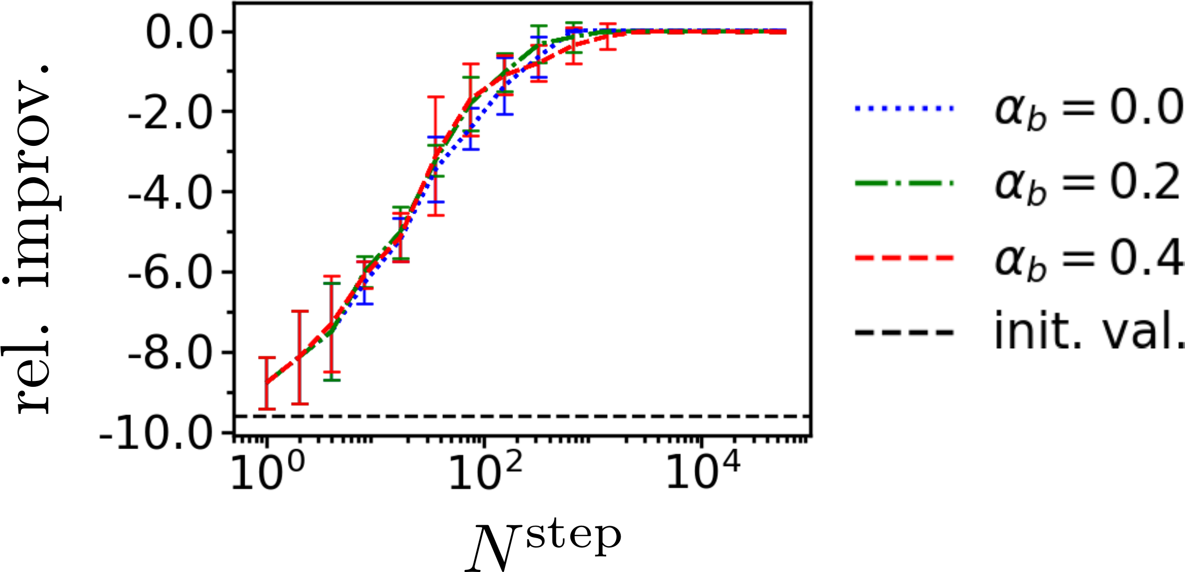
Figure 6: Relative improvement (as defined in Subsec. 3 and estimated from $\Delta G_{\mathrm{solv}}^{\mathrm{cheap}}$) observed at $N^{\mathrm{step}}$ global Monte Carlo steps for QM9* simulations optimizing $\Delta G_{\mathrm{solv}}$ with weak $\Delta\epsilon$ constraint. For each bias proportionality coefficient $\alpha_{b}$ we plot the mean over different random generator seeds, the error bars corresponding to standard deviation. ”init. val.” is the relative improvement of the simulations’ starting molecule, i.e. methane.

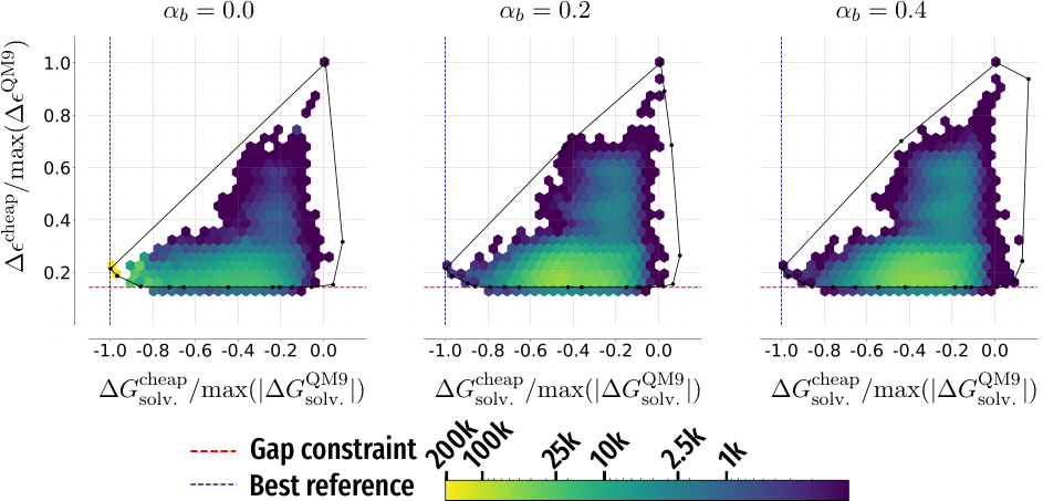
Figure 7: Densities of molecules encountered by example simulations minimizing free energy of solvation $\Delta G_{\mathrm{solv}}$ with weak HOMO-LUMO gap $\Delta\epsilon$ constraint in QM9* for different values of bias proportionality coefficient $\alpha_{b}$.

Optimization in EGP* was harder than in QM9* due to larger size of the former set of molecules, resulting in our protocol generating underconverged simulations that rarely agreed on candidates, producing 83 candidates in total. However, as summarized in Table 2, we still observed significant improvement of optimized quantities compared to EGP, though the improvements’ impressive magnitudes are largely due to EGP containing a much less representative portion of EGP* compared to the case of QM9 and QM9*. Best EGP* candidates for each optimization problem are presented in Figure 8; unlike QM9* candidates, no chemical intuition is seen in how they were constructed beyond adding as many polar covalent bonds as possible, which may be due to underconvergence of our EGP* simulations. The underconvergence can also be observed on our optimization progress plots, the plot for minimizing $\Delta G_{\mathrm{solv}}$ with weak $\Delta\epsilon$ constraint presented in Figure 9 and the rest found in Supporting Information. Figure 9 also demonstrates how adding $\alpha_{b}$ can accelerate optimization as a function of global Monte Carlo steps, though we need to note that simulations with larger $\alpha_{b}$ on average process more chemical graphs per global Monte Carlo steps as discussed in Supporting Information. Densities of molecules encountered during simulations minimizing $\Delta G_{\mathrm{solv}}$ with weak $\Delta\epsilon$ constraint that produced the best candidates are presented in Figure 10; unlike the case of QM9*, increasing $\alpha_{b}$ helped simulations explore parts of chemical space with smaller values of $\Delta G_{\mathrm{solv}}$. Analogous plots for other optimization problems in EGP* are presented in Supporting Information.

optimized	$\Delta\epsilon$	optimized quantity value			relative improvement
quantity	constraint	best	worst		best	worst
$\Delta G_{\mathrm{solv}}$	weak	$-1194\phantom{00}\phantom{.}\pm 7\phantom{000}\phantom{.}$	$-382.2\phantom{0}\pm 1.2\phantom{00}$		$118.0\phantom{0}\pm 0.7\phantom{0}$	$30.84\pm 0.13$
	strong	$-269.8\phantom{0}\pm 2.1\phantom{00}$	$-207.6\phantom{0}\pm 0.9\phantom{00}$		$23.19\pm 0.25$	$15.65\pm 0.11$
$D$	weak	$\phantom{\pm}109.5\phantom{0}\pm 0.9\phantom{00}$	$\phantom{\pm}53.69\pm 0.12\phantom{0}$		$51.16\pm 0.48$	$21.49\pm 0.07$
	strong	$\phantom{\pm}59.81\pm 1.14\phantom{0}$	$\phantom{\pm}25.88\pm 0.17\phantom{0}$		$34.70\pm 0.76$	$11.95\pm 0.12$

Table 2: Best and worst EGP* candidates, data notation is analogous to Table 1. Full list of candidate molecules can be found in Supporting Information.

Figure 8: EGP* candidates that exhibited smallest free energy of solvation $\Delta G_{\mathrm{solv}}$ or largest dipole $D$ under weak or strong constraint on the HOMO-LUMO gap $\Delta\epsilon$. See the Supporting Information for more information about them.

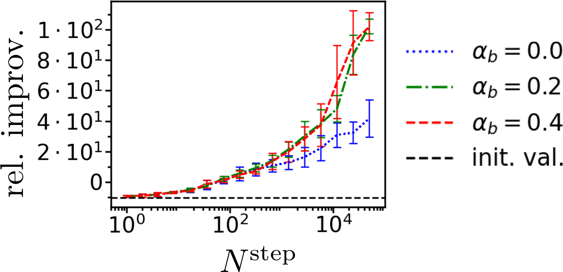
Figure 9: Relative improvement observed at $N^{\mathrm{step}}$ global Monte Carlo steps for EGP* simulations optimizing $\Delta G_{\mathrm{solv}}$ with weak $\Delta\epsilon$ constraint; results are organized analogously to Figure 6.

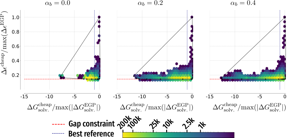
Figure 10: Densities of molecules encountered by simulations minimizing free energy of solvation $\Delta G_{\mathrm{solv}}$ with weak HOMO-LUMO gap $\Delta\epsilon$ constraint in EGP* that produced the candidate with smallest $\Delta G_{\mathrm{solv}}$ for a given value of bias proportionality coefficient $\alpha_{b}$.

4 Conclusions and outlook

We have proposed an effective algorithm for optimization in chemical space, dubbed MOSAiCS, and successfully applied it to several test optimization problems connected to lithium battery electrolyte design. In the current implementation, it is only feasible to optimize estimates of quantities of interest that can be evaluated with little computational effort due to the large number of evaluations of loss function made during a simulation (see Supporting Information); given successes in using active learning for optimization problems in both configuration^{80, 81, 82, 83} and chemical^{84, 85, 58} space, our first priority is to combine MOSAiCS with a similar protocol to decrease the number of loss function evaluations done during the simulations. Successful use of Markov Decision Process formalism to accelerate genetic algorithms in chemical space⁵⁹ suggests MOSAiCS might similarly be improved with a smarter policy for choosing elementary mutations and crossover moves. On a more general note, any method for generating chemical graphs that can also provide corresponding proposition probability $P_{\mathrm{prop}}$ needed for $P_{\mathrm{acc}}$ (4) can be integrated into MOSAiCS framework directly.

While we aimed to propose an approach that would be agnostic to how much is known about the chemical graph set of interest, we still relied on QM9 and EGP to get reasonably rescaled loss functions $F_{\mathrm{solv.}}$ (5) and $F_{\mathrm{dipole}}$ (6) that were then used during simulations in QM9* and EGP*. This dependence on previously published data should become avoidable by implementing more sophisticated schemes⁸⁶ for adjusting temperature parameters $\beta^{(i)}$ based on trajectory history. Also, while we used heavy atoms with connected hydrogens as nodes of chemical graphs to maximize chemical diversity of generated compounds, it is possible to expand the algorithm to using larger compound fragments as nodes instead. If applicable to the optimization problem at hand, this modification should simplify the search by both decreasing effective dimensionality of the graphs considered^{31, 26} and improving scalability of machine learning models for the molecules of interest.^{87, 88}

5 Code availability

Python implementation of MOSAiCS is available at https://github.com/chemspacelab/mosaics.

Details of MOSAiCS implementation and quantity of interest evaluation, discussion of accessibility of QM9* and EGP* by our simulations, additional experimental results.

This project has received funding from the European Union’s Horizon 2020 research and innovation programme under grant agreement No 957189 (BIG-MAP) and No 957213 (BATTERY 2030+). O.A.v.L. has received funding from the European Research Council (ERC) under the European Union’s Horizon 2020 research and innovation programme (grant agreement No. 772834). O.A.v.L. has received support as the Ed Clark Chair of Advanced Materials and as a Canada CIFAR AI Chair. O.A.v.L. acknowledges that this research is part of the University of Toronto’s Acceleration Consortium, which receives funding from the Canada First Research Excellence Fund (CFREF). Obtaining the presented computational results has been facilitated using the queueing system implemented at http://leruli.com. The project has been supported by the Swedish Research Council (Vetenskapsrådet), and the Swedish National Strategic e-Science program eSSENCE as well as by computing resources from the Swedish National Infrastructure for Computing (SNIC/NAISS).

References

- Jafari et al. 2022 Jafari, M.; Botterud, A.; Sakti, A. Decarbonizing power systems: A critical review of the role of energy storage. Renewable Sustainable Energy Rev. 2022, 158, 112077
- Korth 2014 Korth, M. Large-scale virtual high-throughput screening for the identification of new battery electrolyte solvents: evaluation of electronic structure theory methods. Phys. Chem. Chem. Phys. 2014, 16, 7919–7926
- Cheng et al. 2015 Cheng, L.; Assary, R. S.; Qu, X.; Jain, A.; Ong, S. P.; Rajput, N. N.; Persson, K.; Curtiss, L. A. Accelerating Electrolyte Discovery for Energy Storage with High-Throughput Screening. J. Phys. Chem. Lett. 2015, 6, 283–291
- Borodin et al. 2015 Borodin, O.; Olguin, M.; Spear, C. E.; Leiter, K. W.; Knap, J. Towards high throughput screening of electrochemical stability of battery electrolytes. Nanotechnology 2015, 26, 354003
- Qu et al. 2015 Qu, X.; Jain, A.; Rajput, N. N.; Cheng, L.; Zhang, Y.; Ong, S. P.; Brafman, M.; Maginn, E.; Curtiss, L. A.; Persson, K. A. The Electrolyte Genome project: A big data approach in battery materials discovery. Comput. Mater. Sci. 2015, 103, 56–67
- Lian et al. 2019 Lian, C.; Liu, H.; Li, C.; Wu, J. Hunting ionic liquids with large electrochemical potential windows. AIChE J. 2019, 65, 804–810
- Agarwal et al. 2021 Agarwal, G.; Doan, H. A.; Robertson, L. A.; Zhang, L.; Assary, R. S. Discovery of Energy Storage Molecular Materials Using Quantum Chemistry-Guided Multiobjective Bayesian Optimization. Chem. Mater. 2021, 33, 8133–8144
- Sorkun et al. 2019 Sorkun, E.; Zhang, Q.; Khetan, A.; Sorkun, M. C.; Er, S. RedDB, a computational database of electroactive molecules for aqueous redox flow batteries. Sci. Data 2019, 9, 718
- Huang et al. 2023 Huang, B.; von Rudorff, G. F.; von Lilienfeld, O. A. The central role of density functional theory in the AI age. Science 2023, 381, 170–175
- Chang and von Lilienfeld 2018 Chang, K. Y. S.; von Lilienfeld, O. A. crystals with direct 2 eV band gaps from computational alchemy. Phys. Rev. Mater. 2018, 2, 073802
- Griego et al. 2021 Griego, C. D.; Kitchin, J. R.; Keith, J. A. Acceleration of catalyst discovery with easy, fast, and reproducible computational alchemy. Int. J. Quantum Chem. 2021, 121, e26380
- Eikey et al. 2022 Eikey, E. A.; Maldonado, A. M.; Griego, C. D.; von Rudorff, G. F.; Keith, J. A. Evaluating quantum alchemy of atoms with thermodynamic cycles: Beyond ground electronic states. J. Chem. Phys. 2022, 156, 064106
- You et al. 2018 You, J.; Liu, B.; Ying, R.; Pande, V.; Leskovec, J. Graph Convolutional Policy Network for Goal-Directed Molecular Graph Generation. arXiv 2018, 1806.02473
- Zhou et al. 2019 Zhou, Z.; Kearnes, S.; Li, L.; Zare, R. N.; Riley, P. Optimization of Molecules via Deep Reinforcement Learning. Sci. Rep. 2019, 9, 10752
- Ståhl et al. 2019 Ståhl, N.; Falkman, G.; Karlsson, A.; Mathiason, G.; Boström, J. Deep Reinforcement Learning for Multiparameter Optimization in de novo Drug Design. J. Chem. Inf. Model. 2019, 59, 3166–3176
- Khemchandani et al. 2020 Khemchandani, Y.; O’Hagan, S.; Samanta, S.; Swainston, N.; Roberts, T. J.; Bollegala, D.; Kell, D. B. DeepGraphMolGen, a multi-objective, computational strategy for generating molecules with desirable properties: a graph convolution and reinforcement learning approach. J. Cheminform. 2020, 12, 53
- Horwood and Noutahi 2020 Horwood, J.; Noutahi, E. Molecular Design in Synthetically Accessible Chemical Space via Deep Reinforcement Learning. ACS Omega 2020, 5, 32984–32994
- Pereira et al. 2021 Pereira, T.; Abbasi, M.; Ribeiro, B.; Arrais, J. P. Diversity oriented Deep Reinforcement Learning for targeted molecule generation. J. Cheminform. 2021, 13, 21
- Gupta et al. 2018 Gupta, A.; Müller, A. T.; Huisman, B. J. H.; Fuchs, J. A.; Schneider, P.; Schneider, G. Generative Recurrent Networks for De Novo Drug Design. Mol. Inform. 2018, 37, 1700111
- Popova et al. 2019 Popova, M.; Shvets, M.; Oliva, J.; Isayev, O. MolecularRNN: Generating realistic molecular graphs with optimized properties. arXiv 2019, 1905.13372
- Globus et al. 1999 Globus, A.; Lawton, J.; Wipke, T. Automatic molecular design using evolutionary techniques. Nanotechnology 1999, 10, 290
- Brown et al. 2004 Brown, N.; McKay, B.; Gilardoni, F.; Gasteiger, J. A Graph-Based Genetic Algorithm and Its Application to the Multiobjective Evolution of Median Molecules. J. Chem. Inf. Comput. Sci. 2004, 44, 1079–1087
- Virshup et al. 2013 Virshup, A. M.; Contreras-García, J.; Wipf, P.; Yang, W.; Beratan, D. N. Stochastic Voyages into Uncharted Chemical Space Produce a Representative Library of All Possible Drug-Like Compounds. J. Am. Chem. Soc. 2013, 135, 7296–7303
- Jensen 2019 Jensen, J. H. A graph-based genetic algorithm and generative model/Monte Carlo tree search for the exploration of chemical space. Chem. Sci. 2019, 10, 3567–3572
- Nigam et al. 2022 Nigam, A.; Pollice, R.; Aspuru-Guzik, A. Parallel tempered genetic algorithm guided by deep neural networks for inverse molecular design. Digital Discovery 2022, 1, 390–404
- Laplaza et al. 2022 Laplaza, R.; Gallarati, S.; Corminboeuf, C. Genetic Optimization of Homogeneous Catalysts. Chem. Methods 2022, 2, e202100107
- Gómez-Bombarelli et al. 2018 Gómez-Bombarelli, R.; Wei, J. N.; Duvenaud, D.; Hernández-Lobato, J. M.; Sánchez-Lengeling, B.; Sheberla, D.; Aguilera-Iparraguirre, J.; Hirzel, T. D.; Adams, R. P.; Aspuru-Guzik, A. Automatic Chemical Design Using a Data-Driven Continuous Representation of Molecules. ACS Cent. Sci. 2018, 4, 268–276
- Oliveira et al. 2022 Oliveira, A. F.; Da Silva, J. L. F.; Quiles, M. G. Molecular Property Prediction and Molecular Design Using a Supervised Grammar Variational Autoencoder. J. Chem. Inf. Model. 2022, 62, 817–828
- Levin and Peres 2017 Levin, D. A.; Peres, Y. Markov Chains and Mixing Times: Second Edition; American Mathematical Society, 2017
- Fu et al. 2021 Fu, T.; Xiao, C.; Li, X.; Glass, L. M.; Sun, J. MIMOSA: Multi-constraint Molecule Sampling for Molecule Optimization. Proc. Conf. AAAI Artif. Intell. 2021, 35, 125–133
- Xie et al. 2021 Xie, Y.; Shi, C.; Zhou, H.; Yang, Y.; Zhang, W.; Yu, Y.; Lei, L. MARS: Markov Molecular Sampling for Multi-objective Drug Discovery. arXiv 2021, 2103.10432
- Liang and Wong 2000 Liang, F.; Wong, W. H. Evolutionary Monte Carlo: applications to C-p model sampling and change point problem. Stat. Sin. 2000, 10, 317–342
- Hu and Tsui 2010 Hu, B.; Tsui, K.-W. Distributed evolutionary Monte Carlo for Bayesian computing. Comput. Stat. Data Anal. 2010, 54, 688–697
- Spezia 2020 Spezia, L. Bayesian variable selection in non-homogeneous hidden Markov models through an evolutionary Monte Carlo method. Comput. Stat. Data. Anal. 2020, 143, 106840
- Hukushima and Nemoto 1996 Hukushima, K.; Nemoto, K. Exchange Monte Carlo Method and Application to Spin Glass Simulations. J. Phys. Soc. Jpn. 1996, 65, 1604–1608
- Sambridge 2014 Sambridge, M. A Parallel Tempering algorithm for probabilistic sampling and multimodal optimization. Geophys. J. Int. 2014, 196, 357–374
- Angelini and Ricci-Tersenghi 2019 Angelini, M. C.; Ricci-Tersenghi, F. Monte Carlo algorithms are very effective in finding the largest independent set in sparse random graphs. Phys. Rev. E 2019, 100, 013302
- Holland 1975 Holland, J. H. Adaptation in Natural and Artificial Systems; University of Michigan Press, Ann Arbor, 1975
- Jóhannesson et al. 2002 Jóhannesson, G. H.; Bligaard, T.; Ruban, A. V.; Skriver, H. L.; Jacobsen, K. W.; Nøorskov, J. K. Combined Electronic Structure and Evolutionary Search Approach to Materials Design. Phys. Rev. Lett. 2002, 88, 255506
- Sharma et al. 2010 Sharma, S.; Singh, H.; Balint-Kurti, G. G. Genetic algorithm optimization of laser pulses for molecular quantum state excitation. J. Chem. Phys. 2010, 132, 064108
- Hastings 1970 Hastings, W. K. Monte Carlo sampling methods using Markov chains and their applications. Biometrika 1970, 57, 97–109
- Iftimie et al. 2000 Iftimie, R.; Salahub, D.; Wei, D.; Schofield, J. Using a classical potential as an efficient importance function for sampling from an ab initio potential. J. Chem. Phys. 2000, 113, 4852–4862
- Gelb 2003 Gelb, L. D. Monte Carlo simulations using sampling from an approximate potential. J. Chem. Phys. 2003, 118, 7747–7750
- Jadrich and Leiding 2020 Jadrich, R. B.; Leiding, J. A. Accelerating Ab Initio Simulation via Nested Monte Carlo and Machine Learned Reference Potentials. J. Phys. Chem. B 2020, 124, 5488–5497
- Zhang et al. 2013 Zhang, L.; Iyyamperumal, R.; Yancey, D. F.; Crooks, R. M.; Henkelman, G. Design of Pt-Shell Nanoparticles with Alloy Cores for the Oxygen Reduction Reaction. ACS Nano 2013, 7, 9168–9172
- Anderson et al. 2015 Anderson, R. M.; Yancey, D. F.; Zhang, L.; Chill, S. T.; Henkelman, G.; Crooks, R. M. A Theoretical and Experimental Approach for Correlating Nanoparticle Structure and Electrocatalytic Activity. Acc. Chem. Res. 2015, 48, 1351–1357
- Shields et al. 2021 Shields, B. J.; Stevens, J.; Li, J.; Parasram, M.; Damani, F.; Alvarado, J. I. M.; Janey, J. M.; Adams, R. P.; Doyle, A. G. Bayesian reaction optimization as a tool for chemical synthesis. Nature 2021, 590, 89–96
- Park et al. 2023 Park, J.; Kim, Y. M.; Hong, S.; Han, B.; Nam, K. T.; Jung, Y. Closed-loop optimization of nanoparticle synthesis enabled by robotics and machine learning. Matter 2023, 6, 677–690
- Rahmanian et al. 2022 Rahmanian, F.; Flowers, J.; Guevarra, D.; Richter, M.; Fichtner, M.; Donnely, P.; Gregoire, J. M.; Stein, H. S. Enabling Modular Autonomous Feedback-Loops in Materials Science through Hierarchical Experimental Laboratory Automation and Orchestration. Adv. Mater. Interfaces 2022, 9, 2101987
- Stein et al. 2022 Stein, H. S.; Sanin, A.; Rahmanian, F.; Zhang, B.; Vogler, M.; Flowers, J. K.; Fischer, L.; Fuchs, S.; Choudhary, N.; Schroeder, L. From materials discovery to system optimization by integrating combinatorial electrochemistry and data science. Curr. Opin. Electrochem. 2022, 35, 101053
- Manzano et al. 2022 Manzano, J. S.; Hou, W.; Zalesskiy, S. S.; Frei, P.; Wang, H.; Kitson, P. J.; Cronin, L. An autonomous portable platform for universal chemical synthesis. Nat. Chem. 2022, 14, 1311–1318
- Nigam et al. 2021 Nigam, A.; Pollice, R.; Krenn, M.; dos Passos Gomes, G.; Aspuru-Guzik, A. Beyond generative models: superfast traversal, optimization, novelty, exploration and discovery (STONED) algorithm for molecules using SELFIES. Chem. Sci. 2021, 12, 7079–7090
- Born and Manica 2023 Born, J.; Manica, M. Regression Transformer enables concurrent sequence regression and generation for molecular language modelling. Nat. Mach. Intell. 2023, 5, 432–444
- Lemm and von Lilienfeld 2021 Lemm, D.; von Lilienfeld, G. F. v. O. A. Machine learning based energy-free structure predictions of molecules, transition states, and solids. Nat. Commun. 2021, 12, 4468
- Weinreich et al. 2022 Weinreich, J.; Lemm, D.; von Rudorff, G. F.; von Lilienfeld, O. Ab initio machine learning of phase space averages. J. Chem. Phys. 2022, 157, 024303
- Wang and Landau 2001 Wang, F.; Landau, D. P. Efficient, Multiple-Range Random Walk Algorithm to Calculate the Density of States. Phys. Rev. Lett. 2001, 86, 2050–2053
- Thiede et al. 2022 Thiede, L. A.; Krenn, M.; Nigam, A. K.; Aspuru-Guzik, A. Curiosity in exploring chemical spaces: intrinsic rewards for molecular reinforcement learning. Mach. Learn.: Sci. Technol. 2022, 3, 035008
- Reker 2019 Reker, D. Practical considerations for active machine learning in drug discovery. Drug Discov. Today Technol. 2019, 32-33, 73–79
- Fu et al. 2022 Fu, T.; Gao, W.; Coley, C.; Sun, J. Reinforced Genetic Algorithm for Structure-based Drug Design. Advances in Neural Information Processing Systems. 2022; pp 12325–12338
- Carter et al. 2023 Carter, Z. J.; Hollander, K.; Spasov, K. A.; Anderson, K. S.; Jorgensen, W. L. Design, synthesis, and biological testing of biphenylmethyloxazole inhibitors targeting HIV-1 reverse transcriptase. Bioorg. Med. Chem. Lett. 2023, 84, 129216
- Borodin 2019 Borodin, O. Challenges with prediction of battery electrolyte electrochemical stability window and guiding the electrode – electrolyte stabilization. Curr. Opin. Electrochem. 2019, 13, 86–93
- Teunissen et al. 2017 Teunissen, J. L.; De Proft, F.; De Vleeschouwer, F. Tuning the HOMO–LUMO Energy Gap of Small Diamondoids Using Inverse Molecular Design. J. Chem. Theory Comput. 2017, 13, 1351–1365
- De_2020 Do HOMO-LUMO Energy Levels and Band Gaps Provide Sufficient Understanding of Dye-Sensitizer Activity Trends for Water Purification? ACS Omega 2020, 5, 15052–15062
- Fromer and Coley 2023 Fromer, J. C.; Coley, C. W. Computer-aided multi-objective optimization in small molecule discovery. Patterns 2023, 4, 100678
- Halgren 1996 Halgren, T. A. Merck molecular force field. I. Basis, form, scope, parameterization, and performance of MMFF94. J. Comput. Chem. 1996, 17, 490–519
- Halgren 1996 Halgren, T. A. Merck molecular force field. II. MMFF94 van der Waals and electrostatic parameters for intermolecular interactions. J. Comput. Chem. 1996, 17, 520–552
- Halgren 1996 Halgren, T. A. Merck molecular force field. III. Molecular geometries and vibrational frequencies for MMFF94. J. Comput. Chem. 1996, 17, 553–586
- Halgren and Nachbar 1996 Halgren, T. A.; Nachbar, R. B. Merck molecular force field. IV. Conformational energies and geometries for MMFF94. J. Comput. Chem. 1996, 17, 587–615
- Halgren 1996 Halgren, T. A. Merck molecular force field. V. Extension of MMFF94 using experimental data, additional computational data, and empirical rules. J. Comput. Chem. 1996, 17, 616–641
- Halgren 1999 Halgren, T. A. MMFF VI. MMFF94s option for energy minimization studies. J. Comput. Chem. 1999, 20, 720–729
- Halgren 1999 Halgren, T. A. MMFF VII. Characterization of MMFF94, MMFF94s, and other widely available force fields for conformational energies and for intermolecular-interaction energies and geometries. J. Comput. Chem. 1999, 20, 730–748
- Bannwarth et al. 2019 Bannwarth, C.; Ehlert, S.; Grimme, S. GFN2-xTB-An Accurate and Broadly Parametrized Self-Consistent Tight-Binding Quantum Chemical Method with Multipole Electrostatics and Density-Dependent Dispersion Contributions. J. Chem. Theory Comput. 2019, 15, 1652–1671
- Ehlert et al. 2021 Ehlert, S.; Stahn, M.; Spicher, S.; Grimme, S. Robust and Efficient Implicit Solvation Model for Fast Semiempirical Methods. J. Chem. Theory Comput. 2021, 17, 4250–4261
- Ruddigkeit et al. 2012 Ruddigkeit, L.; van Deursen, R.; Blum, L. C.; Reymond, J.-L. Enumeration of 166 Billion Organic Small Molecules in the Chemical Universe Database GDB-17. J. Chem. Inf. Model. 2012, 52, 2864–2875
- Ramakrishnan et al. 2014 Ramakrishnan, R.; Dral, P. O.; Rupp, M.; von Lilienfeld, O. A. Quantum chemistry structures and properties of 134 kilo molecules. Sci. Data 2014, 1, 140022
- Jain et al. 2013 Jain, A.; Ong, S. P.; Hautier, G.; Chen, W.; Richards, W. D.; Dacek, S.; Cholia, S.; Gunter, D.; Skinner, D.; Ceder, G.; Persson, K. A. Commentary: The Materials Project: A materials genome approach to accelerating materials innovation. APL Mater. 2013, 1, 011002
- Clayden et al. 2012 Clayden, J.; Geeves, N.; Warren, S. Organic Chemistry, 2nd ed.; Oxford University Press, 2012
- Rathore et al. 2005 Rathore, N.; Chopra, M.; J. de Pablo, J. Optimal allocation of replicas in parallel tempering simulations. J. Chem. Phys. 2005, 122, 024111
- Kone and Kofke 2005 Kone, A.; Kofke, D. A. Selection of temperature intervals for parallel-tempering simulations. J. Chem. Phys. 2005, 122, 206101
- Gastegger et al. 2017 Gastegger, M.; Behler, J.; Marquetand, P. Machine learning molecular dynamics for the simulation of infrared spectra. Chem. Sci. 2017, 8, 6924–6935
- Podryabinkin and Shapeev 2017 Podryabinkin, E. V.; Shapeev, A. V. Active learning of linearly parametrized interatomic potentials. Comput. Mater. Sci. 2017, 140, 171–180
- Schaaf et al. 2023 Schaaf, L.; Fako, E.; De, S.; Schäfer, A.; Csányi, G. Accurate Reaction Barriers for Catalytic Pathways: An Automatic Training Protocol for Machine Learning Force Fields. arXiv 2023, 2301.09931
- Vandermause et al. 2022 Vandermause, J.; Xie, Y.; Lim, J. S.; Owen, C. J.; Kozinsky, B. Active learning of reactive Bayesian force fields applied to heterogeneous catalysis dynamics of H/Pt. Nat. Commun. 2022, 13, 5183
- Hernández-Lobato et al. 2017 Hernández-Lobato, J. M.; Requeima, J.; Pyzer-Knapp, E. O.; Aspuru-Guzik, A. Parallel and Distributed Thompson Sampling for Large-scale Accelerated Exploration of Chemical Space. arXiv 2017, 1706.01825
- Smith et al. 2018 Smith, J. S.; Nebgen, B.; Lubbers, N.; Isayev, O.; Roitberg, A. E. Less is more: Sampling chemical space with active learning. J. Chem. Phys. 2018, 148, 241733
- Vousden et al. 2005 Vousden, W. D.; Farr, W. M.; Mandel, I. Dynamic temperature selection for parallel tempering in Markov chain Monte Carlo simulations. Mon. Not. R. Astron. Soc. 2005, 455, 1919–1937
- Huang and von Lilienfeld 2020 Huang, B.; von Lilienfeld, O. A. Quantum machine learning using atom-in-molecule-based fragments selected on the fly. Nat. Chem. 2020, 12, 945–951
- Huang et al. 2023 Huang, B.; von Lilienfeld, O. A.; Krogel, J. T.; Benali, A. Toward DMC Accuracy Across Chemical Space with Scalable -QML. J. Chem. Theory Comput. 2023, 19, 1711–1721