Swiper and Dora: efficient solutions to weighted distributed problems

Abstract.

The majority of fault-tolerant distributed algorithms are designed assuming a nominal corruption model, in which at most a fraction $f_{n}$ of parties can be corrupted by the adversary. However, due to the infamous Sybil attack, nominal models are not sufficient to express the trust assumptions in open (i.e., permissionless) settings. Instead, permissionless systems typically operate in a weighted model, where each participant is associated with a weight and the adversary can corrupt a set of parties holding at most a fraction $f_{w}$ of total weight.

In this paper, we suggest a simple way to transform a large class of protocols designed for the nominal model into the weighted model. To this end, we formalize and solve three novel optimization problems, which we collectively call the weight reduction problems, that allow us to map large real weights into small integer weights while preserving the properties necessary for the correctness of the protocols. In all cases, we manage to keep the sum of the integer weights to be at most linear in the number of parties, resulting in extremely efficient protocols for the weighted model. Moreover, we demonstrate that, on weight distributions that emerge in practice, the sum of the integer weights tends to be far from the theoretical worst-case and, often, even smaller than the number of participants.

While, for some protocols, our transformation requires an arbitrarily small reduction in resilience (i.e., $f_{w}=f_{n}-\epsilon$), surprisingly, for many important problems we manage to obtain weighted solutions with the same resilience ($f_{w}=f_{n}$) as nominal ones. Notable examples include asynchronous consensus, verifiable secret sharing, erasure-coded distributed storage and broadcast protocols. Although there are ad-hoc weighted solutions to some of these problems, the protocols yielded by our transformations enjoy all the benefits of nominal solutions, including simplicity, efficiency, and a wider range of possible cryptographic assumptions.

1. Introduction

1.1. Weighted distributed problems

Traditionally, distributed problems are studied in the egalitarian setting where $n$ parties communicate over a network and any $t$ of them can be faulty or corrupted by a malicious adversary. Different combinations of $n$ and $t$ are possible depending on the problem at hand, the types of failures (crash, omission, semi-honest, or malicious, also known as Byzantine), and the network model (typically, asynchronous, semi-synchronous, or synchronous). However, for most distributed protocols, $t$ has to be smaller than a certain fraction of $n$. For example, most practical Byzantine fault-tolerant consensus protocols (Castro et al., 1999; Canetti and Rabin, 1993) can operate for any $t<\frac{n}{3}$. We call such models nominal and use $f_{n}$ to denote their resilience, i.e., a nominal protocol with resilience $f_{n}$ operates correctly as long as less than $f_{n}n$ parties are corrupt, where $n$ is the total number of participants.

However, this simple corruption model is not always sufficient to express the actual fault structure or trust assumptions of real systems. As a result, we see many practical blockchain protocols adopt a more general, weighted model, where each party is associated with a real weight that, intuitively, represents the number of “votes” this party has in the system. The assumption on the number of corrupt parties in this setting is replaced by the assumption that the total weight of the corrupt parties is smaller than a fraction $f_{w}$ of the total weight of all participants. For example, in permissionless systems, the weight can correspond to the amount of “stake” or computational resources a participant has invested in the system and, in the context of managed systems, to a function of the estimated failure probability.

There are two main reasons to adopt the weighted model in the context of blockchain systems. First and foremost, it protects the system from the infamous Sybil attacks, i.e., malicious users registering themselves multiple times in order to obtain multiple identities, thereby surpassing the resilience threshold $f_{n}$. Secondly, it is speculated that users with a greater amount of resources (monetary, computational, or otherwise) invested in the system, and consequently a higher weight, will be more committed to the system’s stability and less likely to engage in malicious behavior.

1.2. Weighted voting and where it needs help

Perhaps, the most prevalent tool used for the design of distributed protocols is quorum systems (Gifford, 1979; Naor and Wool, 1998; Malkhi and Reiter, 1997). Intuitively, to achieve fault tolerance, each “action” is confirmed by a sufficiently large set of participants (called a quorum). Then, if two actions are conflicting or somehow interdependent (e.g., writing and reading a file in a distributed storage system), then the parties in the intersection of the quorums are supposed to ensure consistency. Thus, many distributed protocols can be converted from the nominal to the weighted setting simply by changing the quorum system, i.e., instead of waiting for confirmations from a certain number of parties, waiting for a set of parties with the corresponding fraction of the total weight. We call this strategy weighted voting and it often allows translating protocols from the nominal to the weighted model while maintaining the same resilience (i.e., $f_{w}=f_{n}$) and, in some cases, with virtually no overhead.

However, weighted voting has two major downsides. First and foremost, many protocols rely on primitives beyond simple quorum systems and weighted voting is often not sufficient to translate these protocols to the weighted model. Notable examples include threshold cryptography (Desmedt, 1993; Boldyreva, 2002), secret sharing (Shamir, 1979; Cachin et al., 2002), erasure and error-correcting codes (MacWilliams and Sloane, 1977), and numerous protocols that rely on these primitives.

Another example relevant to blockchain systems is Single Secret Leader Election protocols (Boneh et al., 2020a; Catalano et al., 2022, 2023; Freitas et al., 2023). We use these protocols to illustrate that not all protocols that cannot be easily converted to the weighted model by applying weighted voting belong to the categories mentioned above.

The second drawback of weighted voting is that it requires a careful examination of the protocol in order to determine whether weighted voting is sufficient to convert it to the weighted model, as well as non-trivial modifications to the protocol implementation. It would be much nicer to have a “black-box” transformation that would take a protocol designed and implemented for the nominal model and output a protocol for the weighted model.

1.3. Our contribution

Problem	nominal solutions	weight-reduction algorithm	$f_{w}$	$f_{n}$	worst-case average comm. overhead	worst-case average comp. overhead
Derived Protocols
Efficient Asynchronous State-Machine Replication	(Miller et al., 2016; Duan et al., 2018; Keidar et al., 2021; Danezis et al., 2022; Spiegelman et al., 2022)	Swiper+Dora	$1/3$	$1/3$	$\times\,1.33$ for Broadcast $\times\,2$ for RNG	$\times\,5.33$ for Broadcast $\times\,2$ for RNG
Structured Mempool	(Danezis et al., 2022)	Dora	$1/3$	$1/3$	$\times\,1.33$ for Broadcast	$\times\,5.33$ for Broadcast
Validated Asynchronous Byzantine Agreement	(Cachin et al., 2001; Abraham et al., 2019)	Swiper	$1/3$	$1/3$	$\times\,2$ for RNG	$\times\,2$ for RNG
Consensus with Checkpoints	(Azouvi and Vukolić, 2022)	Swiper	$1/3$	$1/3$	$\times\,2$ for signing	$\times\,2$ for signing
Useful Building Blocks
Erasure-Coded Storage and Broadcast	(Rabin, 1989; Cachin and Tessaro, 2005; Hendricks et al., 2007; Nazirkhanova et al., 2021; Yang et al., 2022; Nayak et al., 2020)	Dora	$1/3$	$1/3$	$\times\,1.33$	$\times\,5.33$
		Swiper (BB)	$1/4$	$1/3$	–	$\times\,3$
Error-Corrected Broadcast	(Das et al., 2021)	Dora	$1/3$	$1/3$	$\times\,1.33$	$\times\,10.66$
		Swiper (BB)	$1/4$	$1/3$	–	$\times\,3$
Blunt Secret Sharing	(Shamir, 1979)	Swiper	$1/3$	$1/3$	$\times\,2$	$\times\,2$
Distributed RNG	(Rabin, 1983; Cachin et al., 2000)
Blunt Threshold Signatures	(Boldyreva, 2002; Stinson and Strobl, 2001; Shoup, 2000)
Blunt Threshold Encryption	(Desmedt, 1993)
Blunt Threshold FHE	(Jain et al., 2017; Boneh et al., 2018)
Tight Secret Sharing	Sec. 5.2 (this paper)	Swiper	$1/3$	$1/3$	$\times\,2$	$\times\,2$
Tight Threshold Signatures
Tight Threshold Encryption
Tight Threshold FHE
Linear BFT Consensus	(Yin et al., 2019)	Swiper (BB)	$1/4$	$1/3$	$\times\,3$	$\times\,3$
Chain-Quality SSLE	(Boneh et al., 2020a)

Table 1. Examples of suggested weighted distributed protocols with the upper bounds on communication and computation overhead compared to the nominal solutions with the same number of participants. See Sections 5, 6 and 7 for details on how these numbers were obtained. In Section 9, we study real-world weight distributions and conclude that, in practice, the overhead should be much smaller. “Swiper” and “Dora” refer to weight-reduction algorithms defined in Section 4 and used to achieve these results. “Swiper (BB)” refers to the black-box transformation described in Section 5.3.

System	Total weight	# parties	# tickets using Swiper
			$\alpha_{w}=1/4$	$\alpha_{w}=1/3$	$\alpha_{w}=1/3$	$\alpha_{w}=2/3$
			$\alpha_{n}=1/3$	$\alpha_{n}=3/8$	$\alpha_{n}=1/2$	$\alpha_{n}=3/4$
Aptos (Aptos, 2022; apt, [n. d.])	$8.4708\times 10^{8}$	$104$	$58$	$203$	$27$	$138$
Tezos (Goodman, 2014; tez, [n. d.])	$6.7579\times 10^{8}$	$382$	$136$	$598$	$75$	$481$
Filecoin (Labs, 2017; fil, [n. d.])	$2.5242\times 10^{19}$	$3700$	$3307$	$11814$	$1895$	$8454$
Algorand (Micali, 2016; alg, [n. d.])	$9.7223\times 10^{9}$	$42~{}920$	$961$	$17273$	$373$	$17222$

Table 2. Number of allocated tickets on sample weight distributions, using the Swiper protocol described in Section 4 with recommended parameters.

Our contribution to the fields of distributed computing and applied cryptography is twofold:

1. We present a simple and efficient black-box transformation that can be applied to convert a wide range of protocols designed for the nominal model into the weighted model. Crucially, one can determine the applicability of our transformation simply by examining the problem that is being solved (e.g., Byzantine consensus) instead of the protocol itself (e.g., PBFT (Castro et al., 1999)) and it does not require modifications to the source code, only a slim wrapper around it. The price to pay for this transformation is an arbitrarily small decrease in resilience ($f_{w}=f_{n}-\epsilon$, where $\epsilon>0$) and an increase in the communication and computation complexities proportional to $O(\frac{f_{w}}{\epsilon})$.

2. Furthermore, by opening the black box and examining the internal structure of distributed protocols, we discover that by combining our transformation with weighted voting, in many cases, we can obtain weighted algorithms without the reduction in resilience ($f_{w}=f_{n}$) and with a very minor performance penalty.

We summarize some examples of our techniques applied to a range of different protocols in Table 1. The last two columns of the table give the upper bound on the overhead of the obtained weighted protocols compared to their nominal counterparts executed with the same number of parties. Note, however, that, in many cases, the overhead applies only to specific parts of the protocol, which may not be the bottlenecks. Thus, further experimental studies may reveal that the real overhead is even lower or non-existent, even with worst-case weight distribution. Columns “$f_{w}$” and “$f_{n}$” specify the resilience of the obtained weighted protocols and the original nominal protocols, respectively. As was discussed before, in most cases, we manage to avoid sacrificing resilience $(f_{w}=f_{n})$.

Furthermore, the main building block of our constructions, the weight reduction problems, may be of separate interests and may have important applications beyond distributed protocols. It is, indeed, an interesting and somewhat counter-intuitive observation that large real weights can be efficiently (in linear time) reduced to small integer weights while preserving the key properties.

1.4. Empirical findings

The performance of the weighted protocols constructed as suggested in this paper is sensitive to the distribution of weights of the participants. While we provide upper bounds and thus analyze our protocols for “the worst distribution possible”, it is interesting whether such bad weight distributions emerge in practice.

In order to study real-world weight distributions, we tested our weight reduction algorithms on the distribution of funds from multiple existing blockchain systems (Aptos, 2022; Goodman, 2014; Labs, 2017; Dogecoin, 2022; Micali, 2016) on systems ranging in size from a hundred parties (apt, [n. d.]; Aptos, 2022) up to multiple tens of thousands (alg, [n. d.]; Micali, 2016).

Roadmap

The paper is organized as follows: we formally define weight reduction problems in Section 2 and provide constructive upper bounds for them in Section 3. We then proceed to present our approximate algorithms in Section 4. Sections 5, 6 and 7 explain how to apply weight reduction to solve various kinds of weighted distributed problems. In Section 8, we study the question of resilience against splitting attacks, and in Section 9, we study the performance of weight reduction on the weight distributions emerging in practice. We discuss related work in Section 10 and conclude the paper in Section 11

2. Weight reduction problems

In this section, we define the key building block to our construction, the weight reduction problems, which is a class of optimization problems that map (potentially, large) real weights $w_{1},\dots,w_{n}\in\mathbb{R}_{\geq 0}$ to (ideally, small) integers weights $t_{1},\dots,t_{n}\in\mathbb{Z}_{\geq 0}$ while preserving certain key properties. For convenience, we use the word “tickets” to denote the units of the assigned integer weights, i.e., if $t_{1},\dots,t_{n}$ is the output of a weight reduction problem, we say that party $i$ is assigned $t_{i}$ tickets.

2.1. Weight Restriction

The first weight reduction problem is Weight Restriction (or simply WR). It is parameterized by two numbers $\alpha_{w},\alpha_{n}\in(0,1)$ and requires the mapping to preserve the property that any subset of parties of weight less than $\alpha_{w}$ obtains less than $\alpha_{n}$ tickets. More formally:

In Section 5, we apply Weight Restriction in order to implement the black-box transformation announced in Section 1.3 as well as weighted versions of secret sharing and threshold cryptography with different access structures.

In Section 3, we will prove the following theorem (with a more precise bound on $T$):

Theorem 2.1 (WR upper bound, simplified).

For any $\alpha_{w},\alpha_{n}\in(0,1)$ such that $\alpha_{w}<\alpha_{n}$: there exists a solution to the Weight Restriction problem with $T=O\left(\frac{n}{\alpha_{n}-\alpha_{w}}\right)$.

2.2. Weight Qualification

The next weight reduction problem we study is Weight Qualification (or simply WQ). It requires the mapping to preserve the property that any subset of parties of weight more than $\beta_{w}$ obtains more than $\beta_{n}$ tickets. In some sense, WQ is the opposite of the Weight Restriction problem discussed above. More formally:

In Section 6, we show how to apply Weight Qualification to implement weighted versions of storage and broadcast protocols that rely on erasure and error-correcting codes for minimizing communication and storage complexity.

Interestingly, there exists a simple reduction between WR and WQ:

Theorem 2.2.

For any $\beta_{w},\beta_{n}\in(0,1)$ and $w_{1},\dots,w_{n}\in\mathbb{R}_{\geq 0}$, the following problems are identical:

1. $WR(1-\beta_{w},1-\beta_{n},w_{1},\dots,w_{n})$

2. $WQ(\beta_{w},\beta_{n},w_{1},\dots,w_{n})$

Proof.

Let us prove that any valid solution to $WR(1-\beta_{w},1-\beta_{n},w_{1},\dots,w_{n})$ is a valid solution to $WQ(\beta_{w},\beta_{n},w_{1},\dots,w_{n})$. The inverse can be proven analogously. Indeed, if $\forall S\subseteq[n]$ such that $w(S)>\beta_{w}W$: $w([n]\setminus S)=W-w(S)<(1-\beta_{w})W$. Hence, $t([n]\setminus S)<(1-\beta_{n})T$ and $t(S)=1-t([n]\setminus S)>\beta_{n}T$. ∎

From Theorems 2.1 and 2.2, we obtain the following:

Corollary 2.3 (WQ upper bound, simplified).

For any $\beta_{w},\beta_{n}\in(0,1)$ such that $\beta_{n}<\beta_{w}$: there exists a solution to the Weight Qualification problem with $T=O\left(\frac{n}{\beta_{w}-\beta_{n}}\right)$.

2.3. Weight Separation

Finally, Weight Separation combines WR and WQ: it has 4 parameters ($\beta_{w}$, $\beta_{n}$, $\alpha_{w}$, and $\alpha_{n}$) and outputs a ticket distribution that guarantees simultaneously the properties of Weight Qualification and Weight Restriction.

Interestingly, in all practical problems that we have considered, either WR or WQ were sufficient, so we have not yet identified good use cases for the more general Weight Separation problem. However, we believe that it is still interesting theoretically and provide a linear upper bound on the total number of tickets for it, as for the other two problems.

Theorem 2.4 (WS upper bound, simplified).

For any $\beta_{w},\allowbreak\beta_{n},\allowbreak\alpha_{w},\allowbreak\alpha_{n}\in(0,1)$ such that $\alpha_{w}<\alpha_{n}$ and $\beta_{n}<\beta_{w}$: there exists a solution to the Weight Separation problem with $T=O\left(\frac{n}{\min\{\alpha_{n}-\alpha_{w},\beta_{w}-\beta_{n}\}}\right)$.

The special case of WS when $\alpha_{n}=\beta_{n}$ was recently considered for implementation of so-called ramp weighted secret-sharing in (Benhamouda et al., 2022). We discuss the relationship between our work and this result in more detail in the related work section.

2.4. Overview of suggested solutions

In Appendix B, we show how to obtain exact solutions to WR using Mixed Integer Programming (MIP) (Conforti et al., 2014), however, such an approach is prohibitively slow for inputs larger than twenty parties as solving a MIP is NP-hard.

Thus, in Section 3, we provide constructive upper bounds on all three weight reduction problems (WR, WQ, and WS) yielding efficient (linear time) algorithms to find small, albeit not necessarily optimal, solutions.

In Section 4, we further build upon the upper bound for Weight Restriction to obtain Swiper – an efficient polynomial-time algorithm that not only produces at most a linear number of tickets in the worst case but also produces very few tickets on practical weight distributions, as will be studied in Section 9.

We also define an algorithm that we dub Dora to solve the WQ problem. Due to Theorem 2.2, Dora is defined simply as Swiper with parameters $\alpha_{w}:=1-\beta_{w}$ and $\alpha_{n}:=1-\beta_{n}$.

We are currently working on an algorithm that would yield the optimal (i.e., the smallest possible, given the restrictions) number of tickets. However, as this algorithm’s running time is still significant, for practical systems of considerable size (thousands of parties), the approximate algorithms presented in this version of the paper will likely be preferable.

3. Upper Bounds

In this section, we provide constructive upper bounds for all three weight reduction problems defined in the previous section. At their core, our bounds are based on a simple divide-and-round technique. However, we then apply the idea of pruning that is not only useful in practice but also improves the theoretical bounds.

3.1. Upper bounds on Weight Restriction

Floor distribution

Let us distribute for each party $i$, $t_{i}=\lfloor w_{i}/X\rfloor$ tickets for some $X$ that we will later select. Consider a set $S$ such that $w(S)<\alpha_{w}$. Then we can bound the number of tickets allocated to it as follows:

$$t(S) =\sum_{i\in S}t_{i}=\sum_{i\in S}\left\lfloor\frac{w_{i}}{X}\right\rfloor\leq\sum_{i\in S}\frac{w_{i}}{X}=\frac{w(S)}{X}<\frac{\alpha_{w}W}{X}$$

On the other hand, we can give a lower bound on the number of tickets allocated to its complement $\overline{S}$:

$$t(\overline{S})=\sum_{i\not\in S}t_{i}=\sum_{i\not\in S}\left\lfloor\frac{w_{i}}{X}\right\rfloor\geq\sum_{i\not\in S}\left(\frac{w_{i}}{X}-1\right)>\frac{(1-\alpha_{w})W}{X}-n$$

Note that, to simplify the resulting bound and make it independent of the weight distribution, we use $n$ as the upper bound for $|\overline{S}|$, which is a slight oversimplification. In order to prove that $t(S)<\alpha_{n}T$, it is sufficient to show that $\frac{t(S)}{t(\overline{S})}<\frac{\alpha_{n}}{1-\alpha_{n}}$. Indeed:

$$t(S)<\alpha_{n}T\Leftrightarrow t(S)<\alpha_{n}(t(S)+t(\overline{S}))\Leftrightarrow\frac{t(S)}{t(\overline{S})}<\frac{\alpha_{n}}{1-\alpha_{n}}$$

By substituting the bounds we have on $t(S)$ and $t(\overline{S})$, we obtain a sufficient condition for the required inequality to hold:

$$\frac{t(S)}{t(\overline{S})}<\frac{\alpha_{n}}{1-\alpha_{n}}$$

$$\Leftarrow\; \frac{\alpha_{w}W}{(1-\alpha_{w})W-nX}\leq\frac{\alpha_{n}}{1-\alpha_{n}}$$

$$\Leftrightarrow\; X\leq\frac{W}{n}\frac{\alpha_{n}-\alpha_{w}}{\alpha_{n}}$$

Hence, setting $X:=\frac{W}{n}\cdot\frac{\alpha_{n}-\alpha_{w}}{\alpha_{n}}$ is sufficient to guarantee that $t(S)<\alpha_{n}T$ and we can obtain our first upper bound on the optimal number of tickets for WR:

$$T=\sum_{i=1}^{n}\left\lfloor\frac{w_{i}}{X}\right\rfloor\leq\frac{W}{X}=\frac{\alpha_{n}}{\alpha_{n}-\alpha_{w}}n$$

We can go slightly further by pruning the solution: we keep the tickets assigned to parties in $S$ and then remove unnecessary tickets from the other parties while maintaining the $t(S)<\alpha_{n}T$ requirement. To this end, we need to find the set $S$ of weight less than $\alpha_{w}W$ that obtains the most tickets by solving Knapsack (Kellerer et al., 2004). Luckily for us, as detailed in Appendix A, in this case, Knapsack can be solved efficiently in time $O(Tn)$ using dynamic programming on profits (Kellerer et al., 2004, Lemma 2.3.2), and we know that $T\leq\frac{\alpha_{w}n}{\alpha_{n}-\alpha_{w}}$. In total, we will assign only $\left\lceil\frac{t(S)}{\alpha_{n}}\right\rceil$ tickets. As $t(S)<\frac{\alpha_{w}W}{X}$ and $t(S)$ is an integer, $t(S)\leq\frac{\alpha_{w}W}{X}-1$. This leads to a slightly improved upper bound on $T$:

$$T=\left\lceil\frac{t(S)}{\alpha_{n}}\right\rceil\leq\left\lceil\frac{\alpha_{w}}{\alpha_{n}-\alpha_{w}}n-\frac{1}{\alpha_{n}}\right\rceil\leq\frac{\alpha_{w}}{\alpha_{n}-\alpha_{w}}n$$

Ceiling distribution

Let us now do a similar study on the ticket distribution where each party $t_{i}$ is assigned $\lceil w_{i}/X\rceil$ tickets.

$$t(S) =\sum_{i\in S}t_{i}=\sum_{i\in S}\left\lceil\frac{w_{i}}{X}\right\rceil\leq\sum_{i\in S}\left(\frac{w_{i}}{X}+1\right)\leq\frac{\alpha_{w}W}{X}+n$$

$$t(\overline{S}) =\sum_{i\not\in S}t_{i}=\sum_{i\not\in S}\left\lceil\frac{w_{i}}{X}\right\rceil\geq\sum_{i\not\in S}\frac{w_{i}}{X}\geq\frac{(1-\alpha_{w})W}{X}$$

Analogously with the floor distribution, we can obtain a sufficient condition to guarantee that $t(S)<\alpha_{n}T$:

$$t(S)<\alpha_{n}T$$

$$\Leftrightarrow\; \frac{t(S)}{t(\overline{S})}<\frac{\alpha_{n}}{1-\alpha_{n}}$$

$$\Leftarrow\; \frac{\alpha_{w}W+nX}{(1-\alpha_{w})W}\leq\frac{\alpha_{n}}{1-\alpha_{n}}$$

$$\Leftrightarrow\; X\leq\frac{W}{n}\frac{\alpha_{n}-\alpha_{w}}{1-\alpha_{n}}$$

Thus, the total number of tickets distributed is at most:

$$T\leq\sum_{i=1}^{n}\left\lceil\frac{w_{i}}{X}\right\rceil\leq\frac{W}{X}+n=\left(\frac{1-\alpha_{n}}{\alpha_{n}-\alpha_{w}}+1\right)n=\frac{1-\alpha_{w}}{\alpha_{n}-\alpha_{w}}n$$

In this case, pruning does not improve the upper bound on $T$.

Upper bound.

Thus, we obtain a final upper bound as the minimum between these two distributions:

Theorem 3.1 (WR upper bound).

For any $\alpha_{w},\alpha_{n}\in(0,1)$ such that $\alpha_{w}<\alpha_{n}$: for any $w_{1},\dots,w_{n}$: there exists a valid solution to the Weight Restriction problem such that:

$$T\leq\frac{\min\{\alpha_{w},1-\alpha_{w}\}}{\alpha_{n}-\alpha_{w}}n$$

3.2. Upper bounds on Weight Qualification

As a result of Theorem 2.2, we can establish the following bound for WQ:

Theorem 3.2 (WQ upper bound).

For any $\beta_{w},\beta_{n}\in(0,1)$ such that $\beta_{n}<\beta_{w}$: for any $w_{1},\dots,w_{n}$: there exists a valid solution to the Weight Qualification problem such that:

$$T\leq\frac{\min\{\beta_{w},1-\beta_{w}\}}{\beta_{w}-\beta_{n}}n$$

3.3. Upper bounds on Weight Separation

Regarding WS, we can apply the same analysis as in Section 3.1 and choose a value of $X$ that satisfies the requirements of both WR and WQ. For simplicity, we do not consider pruning in this case. Hence, we obtain the following theorem:

Theorem 3.3 (WS upper bound).

For any $\alpha_{w},\alpha_{n},\beta_{w},\beta_{n}\in(0,1)$ such that $\alpha_{w}<\alpha_{n}$ and $\beta_{n}<\beta_{w}$: for any $w_{1},\dots,w_{n}\in\mathbb{R}_{\geq 0}$: there exists a valid solution to the Weight Separation problem such that:

$$T\leq\min\left\{T_{floor},T_{ceil}\right\}\text{, where}$$

$$T_{floor}=\max\left\{\frac{\alpha_{n}}{\alpha_{n}-\alpha_{w}},\frac{1-\beta_{n}}{\beta_{w}-\beta_{n}}\right\}n$$

$$T_{ceil}=\max\left\{\frac{1-\alpha_{w}}{\alpha_{n}-\alpha_{w}},\frac{\beta_{w}}{\beta_{w}-\beta_{n}}\right\}n$$

4. Swiper and Dora – efficient solutions to WR and WQ

Swiper is a deterministic approximate algorithm for the Weight Restriction problem. It is designed to not only respect the upper bounds provided in the previous section but also to allocate a small number of tickets on practical weight distributions. The main insight is that the choice of the value $X$ in Section 3.1 is very pessimistic: we choose it based only on the total weight $W$, number of parties $n$, and thresholds $\alpha_{n}$ and $\alpha_{w}$. In Swiper we essentially try all possible values for $X$ and pick the maximum value so that the condition imposed by the WR problem statement is satisfied. We do so in a highly optimized manner.

The full code is available on GitHub. The Python implementation available on GitHub has a parameter --speed that accepts values between 1 and 10. We recommend the value --speed 3 for small systems ($n<1000$) and --speed 5 for larger systems ($n<100^{\prime}000$). Value --speed 7 provides a quadratic solution and --speed 10 provides a linear solution.

In Algorithm 1, we present a simplified version that omits some important optimizations. Nevertheless, its running time is still $O(poly(n))$. We start by picking the value of $X$ as in Section 3.1. This already reduces the total number of tickets to $U=O(n)$.

The protocol proceeds to test all $U$ meaningful values of $X$ that change the ticket distribution, testing validity by solving knapsack (which we remind that for this particular instance can be efficiently computed) and keeping the valid distribution that yields the least amount of tickets as the solution. This search is further sped up by analyzing the values of $X$ that change the number of tickets of parties included in the optimal restriction set since taking tickets out of participants outside this set while keeping the tickets of included parties does not change the number of restricted tickets. Once a solution is found, it is pruned so that the total number of tickets is exactly $\lceil T_{A}/\alpha_{n}\rceil$ by discarding unnecessary tickets of parties not in the restricted set given its optimal choice strategy. We do the computations twice, distributing first $\lfloor w_{i}/X\rfloor$ tickets to each party and then $\lceil w_{i}/X\rceil$, keeping as the final distribution the one that yields the fewest amount of tickets.

In the Python implementation, we speed up the search for the optimal value of $X$ by doing 2 types of binary search before the linear search described above. First, using linear relaxation of Knapsack as the upper bound on the number of tickets in the optimal restriction set and then using the polynomial exact algorithm for Knapsack. We also provide options to disable any of the steps to reduce the computation time of the algorithm at the cost of potentially having more tickets. Crucially, regardless of the selected --speed parameter, our algorithm is deterministic and, thus, can be run independently by each party without a disagreement on the resulting ticket distribution.

Dora.

As stipulated by Theorem 2.2, we can solve the Weight Qualification problem by reducing it to Weight Restriction. Thus, we define our algorithm for solving WQ, called Dora, as: $\textsf{Dora}(\beta_{w},\beta_{n}):=\textsf{Swiper}(1-\alpha_{w},-1\alpha_{n})$.

1:Input:

2:     $w\in\mathbb{R}_{\geq 0}^{n}$  $\alpha_{n}\in[0,1]$  $\alpha_{w}\in[0,\alpha_{n}]$

3:Operation $allocate(w,X,s)$:

4:     if $s={floor}$ then

5:         return $[\;\lfloor w[i]/X\rfloor~{}|~{}i\in\{1,\dots,n\}\;]$      

6:     if $s={ceil}$ then

7:         return $[\;\lceil w[i]/X\rceil~{}|~{}i\in\{1,\dots,n\}\;]$      

8:Operation $prune(t,w,\alpha_{w},\alpha_{n})$:

9:     ${restricted},t^{r}=\Knapsack(w,t_{s}^{\prime},\alpha_{w}W)$

10:     $t^{\prime}\leftarrow t$

11:     decrease $t^{\prime}[i]$ for $i\not\in{restricted}$ until $\sum_{i=1}^{n}t^{\prime}[i]=\lceil\frac{t^{r}}{\alpha_{n}}\rceil$

12:     Return $t^{\prime}$

13:$W\leftarrow\sum_{i=1}^{n}w_{i}$

14:${strategies}\leftarrow\{{floor},{ceil}\}$

15:for $s\in{strategies}$ do

16:     if s = floor then

17:         $X\leftarrow\frac{W}{n}\cdot\frac{\alpha_{n}-\alpha_{w}}{\alpha_{n}}$      

18:     if s = ceil then

19:         $X\leftarrow\frac{W}{n}\cdot\frac{\alpha_{n}-\alpha_{w}}{1-\alpha_{n}}$      

20:     $t_{s}\leftarrow{allocate}(w,X,s)$

21:     $t_{s}^{\prime}\leftarrow t_{s}$

22:     while True do

23:         ${restricted},t_{s}^{r}=\Knapsack(w,t_{s}^{\prime},\alpha_{w}W)$

24:         if $t_{s}^{r}<\alpha_{n}\sum_{i=1}^{n}t_{s}^{\prime}[i]$ then

25:              $t_{s}\leftarrow t_{s}^{\prime}$          

26:         $X^{\prime}\leftarrow$ min val to allocate $t_{s}^{\prime}[i]-1$ for $i\in{restricted}$

27:         $t_{s}^{\prime}\leftarrow{allocate}(w,X^{\prime},n^{*},s)$

28:         if $s={floor}$ and $\sum_{i=1}^{n}t_{s}^{\prime}=0$ then

29:              break          

30:         if $s={ceil}$ and $\sum_{i=1}^{n}t_{s}^{\prime}=n$ then

31:              break               

32:return $\min_{s\in{strategies}}({prune}(t_{s},w,\alpha_{w},\alpha_{n}))$

Algorithm 1 The $Swiper$ protocol.

5. Applications of Weight Restriction

Many distributed protocols, especially in the Byzantine corruption model and the blockchain setting, rely on distributed cryptographic primitives such as secret sharing (Shamir, 1979; Cachin et al., 2002) and threshold signatures (Desmedt, 1993; Stinson and Strobl, 2001; Boldyreva, 2002). Furthermore, threshold signatures form the basis of the most commonly used protocol (Cachin et al., 2000) for the problem of distributed random number generation (also known as threshold coin tossing, random beacon, or common coin), which, in turn, has numerous applications of its own. However, most threshold cryptosystems are based on the idea of splitting a secret key into a number of discrete pieces such that any $t$ out of $n$ pieces are sufficient to reconstruct the secret key or perform operations on it (e.g., create a threshold signature). Therefore, simple weighted voting, as described in Section 1.2, cannot be applied to such systems.

5.1. Blunt Secret Sharing and derivatives

In cryptography, certain actions have an associated access structure $\mathbb{A}$ which determines all sets of parties that are able to perform these actions once they collaborate. Traditional $(n,k)$-threshold systems can be seen as a particular access structure where $\mathbb{A}=\{P\subseteq[n]:|P|\geq k\}$. Analogously, a weighted threshold access structure can be defined as $\mathbb{A}=\{P\subseteq\Pi:\sum_{i\in P}w_{i}\geq\beta\sum_{i\in\Pi}w_{i}\}$.

We can also define the adversary structure $\mathbb{F}\subseteq 2^{\Pi}$, the set of all sets of parties that can be simultaneously corrupted at any given execution. Often, the adversary structure is also defined via a threshold, with a maximum corruptible weight fraction $\alpha$, e.g. $\mathbb{F}=\{P\subset\Pi:\sum_{i\in P}w_{i}\leq\alpha\sum_{i\in\Pi}w_{i}\}$.

While threshold access structures are commonly studied in cryptography and are applied in numerous distributed protocols, in practice, as we discuss in Section 7, it is often sufficient if the access structure provides the following two properties:

• There exists at least one set entirely composed of correct users that belongs to the access structure. This guarantees liveness properties of the accompanying protocol.

• Any set containing only corrupt parties does not belong to the access structure, as this would break safety properties.

Hence, we define a blunt access structure as follows:

Definition 5.1 (Blunt access structure).

Given a set of parties $\Pi$ and the adversary structure $\mathbb{F}\subseteq 2^{\Pi}$, $\mathbb{A}$ is a blunt access structure w.r.t. $\mathbb{F}$ if $(\forall F\in\mathbb{F}:F\not\in\mathbb{A})\text{ and }(\exists A\in\mathbb{A}:A\cap F=\varnothing)$.

The following theorem shows that solving WR is sufficient to implement weighted cryptographic protocols with blunt access structure by reduction to their nominal counterparts.

Theorem 5.2.

Given a set of parties, a nominal threshold access structure protocol $\mathcal{P}$ with threshold value $f_{n}<1/2$, we obtain a blunt threshold access structure w.r.t. a weighted threshold adversarial structure with parameter $f_{w}<f_{n}$ by solving $WR$ with parameters $\alpha_{w}=f_{w}$ and $\alpha_{n}=f_{n}$. This is accomplished by instantiating $\mathcal{P}$ with $\hat{n}=T$ virtual users and allowing party $i$ to control $t_{i}$ of them.

Proof.

By definition of $WR$, once it distributes $T$ tickets, the number of tickets (and, hence, virtual users) allocated to the corrupt parties will be less than $f_{n}T$. Hence, no element of the adversary structure shall appear in the resulting access structure. In addition, honest participants will receive more than $(1-f_{n})T>f_{n}T$ tickets, ensuring that there exists a set of all correct parties in the access structure. ∎

Note that it is crucial for all participants to agree on how many virtual users are assigned to each party as nominal protocols typically assume that the membership is common knowledge. To this end, it is sufficient for all parties to run an agreed upon deterministic weight-restriction protocol.

Among other things, this way, one can obtain weighted versions of secret sharing (Shamir, 1979), distributed random number generation (Cachin et al., 2000), threshold signatures (Boldyreva, 2002), threshold encryption (Desmedt, 1993), and threshold fully-homomorphic encryption (Jain et al., 2017), all with blunt access structures. In the next section, we discuss how to do it for other access structures.

5.2. Tight Secret Sharing and derivatives

Although a blunt access structure is sufficient for a large spectrum of applications, more restrictive access structures are sometimes necessary as well. Here, we present a straightforward approach that involves just one extra round of communication to transform a blunt access structure into a weighted threshold access structure. This means that our construction can be readily utilized in any protocol that already uses threshold cryptography without requiring significant redesign efforts. We showcase the transformation in Algorithm 2 using the particular example of a generic secret sharing scheme with threshold $\alpha$.

33:$\{t_{1},\dots,t_{n}\}\leftarrow\mathit{WR}(\{w_{1},\dots,w_{n}\},f_{w},f_{n})$

34:$T\leftarrow\sum_{i=1}^{n}t_{i}$

35:Operation Share$(m,\{w_{1},\dots,w_{n}\})$:  

// Executed by dealer.

36:     $\{s_{1}^{1},\dots,s_{1}^{t_{1}},\dots,s_{n}^{1},\dots,s_{n}^{t_{n}}\}\leftarrow(\lceil f_{n}T\rceil,T)$-$\mathit{share}(m)$

37:     $\forall j\in[n]:$ send $\langle\text{SHARES}:s_{i}^{1},\dots,s_{i}^{t_{i}}\rangle$ to party $i$

38:Operation RETRIEVE:  

// Executed by the parties.

39:     Send $\langle{\text{REQUEST}}\rangle$ to all parties

40:Upon receiving $\langle{\text{REQUEST}}\rangle$ from party $j$:

41:     // $w_{req}$ is initially $0$

42:     $w_{req}\leftarrow w_{req}+w_{j}$

43:     if $w_{req}\geq\alpha\sum_{i=1}^{n}w_{i}$ then

44:         send shares received from the dealer to all parties      

45:Upon receiving $\lceil f_{n}T\rceil$ shares:

46:     Reconstruct message $m$

Algorithm 2 Blunt to weighted access structure for party $i$

In order to obtain the weighted access structure, the first step is to compute how many shares need to be dealt to each party by solving the Weight Restriction problem. Using the nominal secret sharing operations, we generate shares for the input message by treating each ticket as a “virtual user”, setting the total number of shares to the total number of tickets, and using the parameter $f_{n}$ to set the reconstruction threshold. The dealer then sends to each party the number of shares determined by the solution to WR.

In the reconstruction phase, each party keeps track of the total weight of parties that have requested the reconstruction. Once the established threshold is surpassed, the participants transmit the shares of the secret that they previously received from the dealer. Finally, the secret is reconstructed once the threshold is surpassed.

The correctness of this transformation comes from the fact that before parties corresponding to at least a fraction $\alpha$ of the total weight request the reveal of the secret, the honest parties do not send their shares, prohibiting the reconstruction of the secret as the shares of corrupted parties are not sufficient, by design, to perform this action. However, once this threshold is surpassed, all honest parties send their shares, and the secret is eventually retrieved, as their shares are, once again, by design, sufficient to surpass the threshold of the nominal secret sharing scheme.

Beyond simple secret sharing, one can obtain weighted versions of the same set of protocols as was discussed at the end of Section 5.1, but with arbitrary access structures.

5.3. Black-Box transformation

The same approach of allocating a number of virtual users according to the number of tickets as described in Section 5.1 can be applied to arbitrary distributed protocols. Intuitively, a distributed protocol $\mathcal{P}$ with resilience $f_{n}$ ($f_{w}$) in the nominal (weighted) model must solve the stated problem iff less than $f_{n}n$ parties (parties with weightless than $f_{w}W$) are corrupted. Hence, by applying the “virtual users” approach, we can essentially emulate the nominal model in the weighted one as long as $f_{w}<f_{n}$. However, as we demonstrate later in this section on the example of the Single Secret Leader problem, this approach has its limitations with respect to what kinds of distributed problems can be solved with it.

We illustrate the black-box transformation with two examples, showing first an example where it works smoothly and then an example where we have to slightly relax the problem statement for it to be applicable.

Linear BFT consensus.

One of the major contributions of the Hotstuff protocol (Yin et al., 2019) was to achieve linear communication complexity BFT consensus. This result was achieved by designing the communication of the protocol in a star pattern, where each participant only communicates with the leader. Thus, in order for the leader to demonstrate that its proposal was accepted by a quorum of replicas, the protocol uses threshold signatures which guarantee that a valid signature can only be generated by combining at least $n-f$ shares. This guarantees that incompatible values are never both validated by a quorum since they shall intersect in at least $f+1$ replicas and at least one of them will be correct, which cannot happen since honest replicas do not vote for different values.

In this case, we cannot apply either of the construction Section 5.1 as we need a tight access structure for the threshold signature, nor can we apply the construction of Section 5.2 as it would make the communication complexity quadratic whereas the main goal of Hotstuff is to keep it linear. However, what we can do is simply apply the virtual users approach in a black-box manner: pick any threshold $f_{w}<f_{n}$, run a deterministic WR protocol, and determine how many virtual identities should each party assume.

Single Secret Leader Election.

SSLE (Boneh et al., 2020b) is a distributed protocol that has as an objective to select one of the participants to be a leader with an additional constraint that only the elected party knows the result of the election. Then, once the leader is ready to make a proposal, it reveals itself and other participants can then correctly verify that the claiming leader was indeed elected by the protocol.

The original paper contains nominal solutions for the protocol relying on ThFHE (Boneh et al., 2018) and on shuffling a list of commitments under the DDH assumption. The authors initially suggest that their protocols could support weights by replicating each party to match their weights. As already discussed, this would create a huge overhead in the protocol for systems with large total weight.

Interestingly, in the original protocol, it is required for the election to be fair, that is, for the probability of each party being elected to be uniform. One could think however of an alternative formulation to the protocol where chain-quaility is required instead, where we might specify that the fraction of blocks produced by corrupt parties should not surpass $f_{n}$ when the adversary might control a fraction of the weights up to $f_{w}$. In this case, we can thus simply apply WR with parameters $\alpha_{w}=f_{w},\alpha_{n}=f_{n}$, immediately guaranteeing such a notion.

Properties such as fairness are one of the limitations of our transformations, since any property that is a function of the weight of the parties will not be preserved after the transformation is applied.

6. Applications of Weight Qualification

6.1. Erasure-Coded Storage and Broadcast

Erasure-coded storage systems (Rabin, 1989; Cachin and Tessaro, 2005; Hendricks et al., 2007; Nazirkhanova et al., 2021; Yang et al., 2022), also known under the names of Information Dispersal Algorithms (IDA) (Rabin, 1989) and Asynchronous Verifiable Information Dispersal (AVID) (Cachin and Tessaro, 2005), are crucial to many systems for space-efficient, secure, and fault-tolerant storage and load balancing. Moreover, as demonstrated in (Cachin and Tessaro, 2005), they can yield highly communication-efficient solutions to the very important problem of asynchronous Byzantine Reliable Broadcast (Cachin et al., 2011; Bracha and Toueg, 1985), a fundamental building block in distributed computing that, among other things, serves as the basis for many practical consensus (Miller et al., 2016; Duan et al., 2018; Keidar et al., 2021; Danezis et al., 2022; Spiegelman et al., 2022), distributed key generation (Abraham et al., 2021; Das et al., 2022), and mempool (Danezis et al., 2022) protocols.

The challenge of applying these protocols in the weighted setting is that $(k,m)$ erasure coding, by definition, converts the original data into $m$ discrete fragments such that any $k$ of them are sufficient to reconstruct the original information. Thus, each party will inevitably get to store an integer number of these fragments, and the smaller $m$ is, the more efficient the encoding and reconstruction will be. Moreover, for the most commonly used codes–Reed Solomon–the original message must be of size at least $k\log m$ bits. Hence, using a large $m$ may lead to increased communication as the message may have to be padded to reach this minimum size. As we illustrate in this section, determining the smallest “safe” number of fragments to give to each party is exactly the WQ problem, solved by Dora.

Let us consider the example of (Cachin and Tessaro, 2005) as it is the first erasure-coded storage protocol tolerating Byzantine faults. We believe Dora can be applied analogously to other similar works.

This protocol operates in a model where any $t$ out of $n$ parties can be malicious or faulty, where $t<\frac{n}{3}$. In other words, it has the nominal fault threshold of $f_{n}=\frac{1}{3}$. The protocol encodes the data using $(t+1,n)$ erasure coding, and the data is considered to be reliably stored once at least $2t+1$ parties claim to have stored their respective fragments. The idea is that, even if $t$ of them are faulty, the remaining $t+1$ parties will be able to cooperate to recover the data.

In order to make a weighted version of this protocol, instead of waiting for confirmations from $2t+1$ parties, one needs to wait for confirmations from a set of parties that together possess more than a fraction $2f_{w}$ of total weight, where $f_{w}=f_{n}=\frac{1}{3}$. A subset of weight less than $f_{w}$ of these parties may be faulty. Hence, for the protocol to work, it is sufficient to guarantee that any subset of total weight more than $2f_{w}-f_{w}=f_{w}$ gets enough fragments to reconstruct the data. To this end, we can apply the WQ problem with the threshold $\beta_{w}=f_{w}$. We can set $\beta_{n}$ to be an arbitrary number such that $0<\beta_{n}<\beta_{w}$. Then, we can use $(\lceil\beta_{n}T\rceil,T)$ erasure coding, where $T$ is the total number of tickets allocated by the WQ solution. Hence, whenever a set of weight more than $2f_{w}$ of parties claim to have stored their fragments, we will be able to reconstruct the data with the help of the correct participants in this set. As for the rest of the protocol, it can be converted to the weighted model simply by applying weighted voting, as was discussed in Section 1.2.

As a result, we manage to obtain a weighted protocol for erasure-coded verifiable storage with the same resilience as in the nominal protocol ($f_{w}=f_{n}=\frac{1}{3}$). The “price” we pay is using erasure coding with a smaller rate ($\beta_{n}$ instead of $f_{w}$), i.e., storing data with a slightly increased level of redundancy. However, note that $\beta_{n}$ can be set arbitrarily close to $f_{w}$, at the cost of more total tickets and, hence, more computation.

Example instantiations

The communication and storage complexity of these protocols depends linearly on the rate of the erasure code. Using Reed-Solomon with Berlekamp-Massey decoding algorithm, the decoding computation complexity (Garrammone, 2013) is $O(m^{2}\cdot\frac{M}{rm})=O(\frac{m}{r}\cdot M)$, where $M$ is the size of the message (which we do not affect), $r$ is the rate of the code (in our case, $r=\beta_{n}$), and $m$ is the number of fragments (in our case, the number of tickets allocated by the solution to the WQ problem). For the sake of illustration, let us fix $\beta_{n}$ to be $\frac{1}{4}$. Then, the rate of the code used in the weighted solution will be $\frac{4}{3}$ times smaller than in the nominal solution. For the number of fragments $m$, let us substitute the upper bound from Section 3.2 ($m\leq\frac{\min\{\beta_{w},1-\beta_{w}\}}{\beta_{w}-\beta_{n}}n$). For $\beta_{w}=\frac{1}{3}$ and $\beta_{n}=\frac{1}{4}$, $m\leq 4n$. Hence, the overall slow-down compared to the nominal solution is $4\cdot\frac{4}{3}\approx 5.33$.

One can also consider using FFT-based decoding algorithms (Justesen, 1976). Since the complexity of the FFT-based decoding depends only polylogarithmically on the number of fragments $m$, one can select the rate of the code ($r=\beta_{n}$) to be much closer to $\beta_{w}$ and, thus, minimize communication and storage overhead.

Some protocols (Nayak et al., 2020) are designed for higher reconstruction thresholds, which allows them to be more communication- and storage-efficient compared to (Cachin and Tessaro, 2005). For these cases, we will need to set $\beta_{w}:=\frac{2}{3}$. By setting $\beta_{n}:=\frac{1}{2}$ and applying the upper bound from Section 3.2, we will obtain the same reduction of factor $\frac{4}{3}$ in rate and $2$ times fewer tickets: $m\leq\frac{\min\{2/3,1-2/3\}}{2/3-1/2}n=2n$. The computational overhead will be $2\cdot\frac{4}{3}\approx 2.66$.

6.2. Error-Corrected Broadcast

The exciting work of (Das et al., 2021) illustrated how one can avoid the need for complicated cryptographic proofs in the construction of communication-efficient broadcast protocols by employing error-correcting codes, thus enabling a better communication complexity when a trusted setup is not available. The protocol of (Das et al., 2021) can be used for the construction of communication-efficient Asynchronous Distributed Key Generation (Abraham et al., 2021; Das et al., 2022) protocols.

Similarly to erasure codes, error-correcting codes convert the data into $m$ discrete fragments, such that any $k$ of them are sufficient to reconstruct the original information. However, they have the additional property that the data can be reconstructed even when some of the fragments input to the decoding procedure are invalid or corrupted. Reed-Solomon decoding allows correcting up to $e$ errors when given $k+2e$ fragments as input.

The protocol of (Das et al., 2021) tolerates up to $t$ failures in a system of $n\geq 3t+1$ parties (for simplicity, we will consider the case $n=3t+1$). Its key contribution is the idea of online error correction. Put simply, the protocol first ensures that:

• Every honest party obtains a cryptographic hash of the data to be reconstructed;

• Every honest party obtains its chunk of the data.

Then, in order to reconstruct a message, an honest party solicits fragments from all other parties and repeatedly tries to reconstruct the original data using the Reed-Solomon decoding and verifies the hash of the output of the decoder against the expected value. As the protocol uses $k=t+1$ and $m=n$, after hearing from all $2t+1$ honest and $e\leq t$ malicious parties, it will be possible to reconstruct the original data (as $2t+1+e\geq k+2e$, for $k=t+1$).

To convert this protocol into the weighted model, it is sufficient to make sure that all honest parties together possess enough fragments to correct all errors introduced by the corrupted parties. To this end, we will apply the WQ problem. We will set $\beta_{w}$ to the fraction of weight owned by honest parties, i.e., $\beta_{w}:=1-f_{w}=\frac{2}{3}$ (where $f_{w}$ will be the resilience of the resulting weighted protocol, $f_{w}=f_{n}=\frac{1}{3}$). However, it is not immediately obvious how to set $\beta_{n}$ to allow the above-mentioned property.

If we want to use error-correcting codes with rate $r$, we need to guarantee that the fraction of fragments received by the honest parties (which is at least $\beta_{n}$) is at least $r+e$, where $e$ is the fraction of fragments received by the corrupted parties. However, since honest parties get at least the fraction $\beta_{n}$ of all fragments, then $e\leq 1-\beta_{n}$. Hence, we need to set $\beta_{n}$ so that $\beta_{n}\geq r+(1-\beta_{n})$. We can simply set $\beta_{n}:=\frac{r}{2}+\frac{1}{2}$ for arbitrary $r<\frac{1}{3}$.

Example instantiation

For the sake of an example, we can set $\beta_{w}:=\frac{2}{3}$, $r:=\frac{1}{4}$ and $\beta_{n}:=\frac{5}{8}$. Then, using the bound from Section 3.2, the number of tickets will be at most $\frac{1-\beta_{w}}{\beta_{w}-\beta_{n}}\cdot n=8n$.

As was discussed above, for erasure codes, we can either use the Berlekamp-Massey decoding algorithm or the FFT-based approaches. The same applies to error-correcting codes. As most practical implementations use the former, we will focus on it. In this case, the communication overhead will be $\frac{r_{n}}{r_{w}}$, where $r_{n}=\frac{1}{3}$ is the rate used in the nominal protocol and $r_{w}$ is the rate used for the weighted protocol (in the example above, $r=\frac{1}{4}$). The computation overhead is $\frac{r_{n}}{r_{w}}\cdot\frac{T}{n}$, where $T$ is the number of tickets allocated by the WQ solution (in the example above, $T\leq 8n$). Hence, for the example parameters, the worst-case computational overhead is $\frac{4}{3}\cdot 8\approx 10.66$.

7. Derived Applications

In this section, we discuss indirect applications of weight reduction problems that are obtained by using one or multiple building blocks discussed in Sections 5 and 6. Crucially, for all applications discussed here, we manage to avoid losing resilience despite applying weight reduction. In all cases, the bulk of the protocol should be converted to the weighted model by applying weighted voting, as discussed in Section 1.2.

Asynchronous State Machine Replication

For asynchronous state machine replication protocols (Miller et al., 2016; Duan et al., 2018; Keidar et al., 2021; Danezis et al., 2022; Spiegelman et al., 2022), we simply need to use a weighted communication-efficient broadcast protocol (discussed in Section 6) and weighted distributed random number generation (discussed in Section 5.1). Crucially, the distributed number generation part can use a nominal protocol with threshold $\alpha_{n}=\frac{1}{2}$ and set $\alpha_{w}:=\frac{1}{3}$, which is the resilience of the rest of the protocol. Thus, in some sense, we level the resilience of different parts of the protocol, without affecting the resilience of the composition.

Validated Asynchronous Byzantine Agreement

The same approach can be applied to generate randomness for Validated Asynchronous Byzantine Agreement (VABA) (Cachin et al., 2001; Abraham et al., 2019).

These protocols also require tight threshold signatures. However, in practice, multi-signatures (Ohta and Okamoto, 1999; Boldyreva, 2002) can be applied instead as they have almost no overhead over threshold signatures on the system sizes where such protocols could be applied (below 1000 participants): it suffices to append the multi-signature with an array of $n$ bits, indicating the set of parties that produced the signature. Then, along with the verification of the validity of the multi-signature itself, anyone can verify that the signers together hold sufficient weight.

Alternatively, one could apply the approach described in Section 5.2 to implement tight weighted threshold signatures. However, it would lead to an increase in message complexity of the resulting protocol, which we want to avoid.

Finally, an ad-hoc weighted threshold signature scheme can be applied, such as the one recently proposed in (Das et al., 2023). Note that these signatures cannot be used for distributed randomness generation as they lack the necessary uniqueness property, and thus we still need to apply Swiper to obtain a complete protocol.

Consensus with Checkpoints

We can apply the same approach for checkpointing proof-of-stake consensus protocols (Azouvi and Vukolić, 2022), but this time for blunt threshold signatures (as discussed in Section 5.1) instead of random number generation. If, for some reason, one wants to use a tight threshold signature, the approach described in Section 5.2 can be applied at the cost of just 1 additional message delay per checkpoint.

Compared to ad-hoc solutions for weighted threshold signatures (Das et al., 2023), we claim that our approach is more computationally efficient as it is basically as fast as the underlying nominal protocol. For example, 1 pairing to verify a BLS signature (Boldyreva, 2002) compared to 13 pairings to verify a signature in (Das et al., 2023). Moreover, the weight reduction approach is more general and can support other types of threshold signatures, such as RSA (Shoup, 2000) and Schnorr (Stinson and Strobl, 2001), the latter being particularly important in the context of checkpointing to Bitcoin (Azouvi and Vukolić, 2022).

8. Splitting Attacks

We claim that the total number of tickets distributed by our protocol is a function of the number of parties in the system and not its total weight. From the results we obtained so far, however, it might seem that an adversary who controls an amount $\alpha_{w}W$ of weight is able to split itself into $\lfloor\alpha_{w}W\rfloor$ parties, making the number of participants of the system a function of the total weight and thus nullifying our claim. We call such an attack a Splitting Attack, as defined in definition 8.1.

Definition 8.1 (Splitting attack on a weight reduction protocol).

Given a system of $n_{H}$ parties with weights $w_{1}^{\prime},w_{2}^{\prime},\dots,w_{n_{H}}^{\prime}$, the adversary includes as many participants as it wants into the system, with the constraint that the sum of the weight of these new participants is at most $\frac{f_{w}}{1-f_{w}}\sum_{i=1}^{n_{H}}w_{i}^{\prime}$. The parties are shuffled and relabeled into a list with weights $w_{1},w_{2},\dots,w_{n}$, which shall correspond to the input of the weight reduction protocol.

This definition is natural, as it only reiterates the fact that the adversary controls a fraction $f_{w}$ of the system weight, but that its goal here is to increase the number of parties in the system. Notice also that it is also equivalent to the scenario where the adversary first corrupts a set of parties and then redistributes the weight into several entities, but the proposed formulation will, in our opinion, make the later analysis easier to follow. We then define splitting resistance in definition 8.2.

Definition 8.2 (Splitting-resistant weight reduction).

A weight reduction algorithm is splitting-resistant if the total number of tickets and the complexity of the algorithm is ${poly}(n_{H})$.

Let us show that any optimal solution to $WR$, as well as the division approach, are both splitting resistant. Suppose that our input was compromised by a splitting attack. The actual number of honest participants, $n_{H}$ is unknown, but it is possible to find a lower bound for it. WLOG, let us suppose that the parties are sorted in decreasing weight order, then let us define $n^{*}$ as the following:

$$\sigma(\eta)=\sum_{i=\eta}^{n}w_{i}$$

$$n^{*}=min(\{\eta|\sigma(\eta)\leq f_{w}\sigma(1)\})$$

That is, $n-n^{*}+1$ is the maximum number of participants that can be corrupted at the same time by the adversary, obtained by taking the corruption set as the parties with the smallest weight possible. For this reason, if the input is the result of a splitting attack on the system, then this number is an upper bound at the number of parties included by the adversary. Equivalently, $n^{*}-1$ is a lower bound on the number of honest parties in the system.

We can fix the number of tickets assigned to parties from $p_{n^{*}}$ to $p_{n}$ zero. Then, we can solve WR on the remaining parties by adjusting the restriction threshold to a new value $\alpha_{w}^{\prime}$. If the original problem had parameter $\alpha_{w}$, then in terms of absolute weight, the threshold was $\alpha_{w}W$. The weight of the system becomes $W^{\prime}=W-\sum_{i=n^{*}}^{n}w_{i}$, thus in order to keep the semantics of the problem correct, we need that $\alpha_{w}^{\prime}W^{\prime}=\alpha_{w}W$.

Since we require $\alpha_{w}^{\prime}<\alpha_{n}$ for the problem to be solvable with arbitrary inputs, we have that:

$$\alpha_{w}^{\prime}=\alpha_{w}\frac{W}{W^{\prime}}\leq\frac{\alpha_{w}}{1-f_{w}}$$

Therefore, as long as $\alpha_{w}\leq(1-f_{w})f_{n}$, a solution to $WR(\{w_{i}\}_{i=1}^{n^{*}-1},\allowbreak\alpha_{w}^{\prime},\alpha_{n})$ is a valid splitting resistant solution to $WR(\{w_{i}\}_{i=1}^{n},\alpha_{w},\alpha_{n})$.

9. Analyzing Weight Restriction on sample systems

(a) Influence of threshold parameters

(b) Influence of the number of parties

Figure 1. Experiment results using Tezos

Experiment description.

We performed two kinds of experiments on real blockchain data. In the first experiment, shown in Figure 1(a), we analyzed the influence of the choice of parameters $\alpha_{w}$ and $\alpha_{n}$ for the original data retrieved from the blockchains; the value of $\alpha_{n}$ was varied in the range $[0.1,1]$, while the value of $\alpha_{w}$ was tested in the range $[0.1\times\alpha_{n},0.9\times\alpha_{n}]$. In the experiments showcased in Figure 1(b), we kept these parameters fixed and analyzed the influence of the number of parties in the metrics we tracked. In order to have the same blockchain with different numbers of parties, we have used a bootstrapping statistical technique where we performed $1000$ experiments sampling parties with replacement from the blockchain data and taking the average of the results.

In each experiment, we tracked the total number of tickets distributed, the maximum number of tickets held by a single party, and the number of parties that get at least one ticket (in the experiments we label them as the number of holders). In Figure 1, we show the results for the Tezos blockchain, but the results for Algorand, Aptos, and Filecoin are also available in Appendix C. The analysis of the results reveals the following information: the upper bound given is very pessimistic, with the total number of tickets very rarely surpassing the number of parties for different values of $\alpha_{n},\alpha_{w}$. The total number of tickets varies extremely close to a linear function on the number of parties, as well as the number of holders. The maximum number of tickets, on the other hand, seems to saturate when the number of parties in absolute terms surpasses the order of magnitude of $1000$, remaining almost constant after that point.

10. Related Work

The simplest solution for creating a weighted threshold cryptographic system is to simply have a user of weight $w$ to become $w$ virtual users and to give one key to each of them. Shamir’s paper describing his secret sharing scheme (Shamir, 1979) puts forward this solution. However, in practice, the total weight tends to be prohibitively large, and quantizing it requires solving weight reduction problems, which is the main subject of this paper.

There is a large body of work studying ad-hoc weighted cryptographic protocols (Garg et al., 2022; Beimel and Weinreb, 2006; Chaidos and Kiayias, 2021; Ito et al., 1989; Das et al., 2023; Benhamouda et al., 2022). Compared to these works, the weight reduction approach studied in this paper has a number of benefits, such as simplicity, efficiency, wider applicability, and a wider range of possible cryptographic assumptions. Moreover, in many cases, ad-hoc solutions can be combined with and benefit from weight reduction.

A recent work (Benhamouda et al., 2022) mentioned a similar idea of reducing real weights to integers to construct ramp secret sharing. This project has been started and the first versions of Swiper have been drafted before the online publication of (Benhamouda et al., 2022). As the main focus of (Benhamouda et al., 2022) is different, we believe that we do a much more in-depth exploration of this direction by studying different kinds of weight reduction problems and their applications beyond secret sharing and suggesting protocols that are not only linear in the worst case, but also allocate very few tickets in empirical evaluations on real-world weight distributions.

11. Concluding remarks

In this paper, we have presented a family of optimization problems called weight reduction that, to the best of our knowledge, has not been studied before. We provided practical protocols to find good, albeit not optimal, solutions to these problems. As we have shown, it allows us to efficiently solve many weighted distributed problems.

We are currently working on polynomial exact solutions to the weight reduction problems, i.e., algorithms that would always yield the minimum possible number of tickets for any given weight distribution. Nevertheless, fast approximate algorithms will remain relevant for large systems.

The discussion we present is extensive but not yet complete. Many interesting questions remain to be answered. Among them is the full formal characterization of problems that can be solved by our transformations. We have also only considered threshold adversaries. Other forms of corruption remain to be considered.

One important aspect of proof-of-stake blockchains is the distribution of incentives, which should depend on the weight of each party, hence meriting further discussion in future work. This combines with a discussion of other adversarial models where all participants are rational, and there is no honest majority.

The behavior of adversaries against a protocol is also interesting. We have discussed the splitting attack and have shown that, under some conditions, the number of tickets produced is upper bound by a function of the number of honest parties. However, as seen in the empirical performance of the protocol, the weight distribution affects the resulting number of tickets. Hence, it is interesting to study how much the performance of the resulting protocols can be affected by the adversary redistributing its stake in the worst possible way, not to gain more tickets, but to increase the total number of tickets in the system, and thus compromise the performance.

Appendix A Solving Knapsack

The $\Knapsack$ problem is a very well-known and studied optimization problem. Methods used to solve it include mixed integer programming, branch and bound, and dynamic programming. In this paper, we will be required to solve $\Knapsack$, which is generally an NP-complete problem. However, as we shall shortly prove in Section 3, the number of keys distributed in an optimal $Weightreductionproblem$ solution is $O(n)$, which will allow us to solve our $\Knapsack$ instances in $O(n^{2})$ time by running dynamic programming by profits. For completeness, and because one of our solutions to weight reduction solutions heavily rely on it, we present this $\Knapsack$ solution in Algorithm 3. More detailed explanations and correctness analysis can be found in (Kellerer et al., 2004).

47:Input:

48:     $C\in\mathbb{R}_{\geq 0}$ – capacity

49:     $w\in\mathbb{R}_{\geq 0}^{n}$ – weights

50:     $k\in\mathbb{Z}_{\geq 0}^{n}$ – profits (keys in our use case)

51:     $U\in\mathbb{Z}_{\geq 0}$ – upper bound on solution

52:${dp}[0]\leftarrow 0$

53:for $q\leftarrow 1$ to $U$ do

54:     ${dp}[q]\leftarrow\infty$

55:for $j\leftarrow 1$ to $n$ do

56:     for $q\leftarrow U$ down to $k[j]$ do

57:         if ${dp}[q-k[j]]+w[j]<{dp}[q]$ then

58:              ${dp}[q]\leftarrow{dp}[q-k[j]]+w[j]$               

59:Return $\max\{q|{dp}[q]\leq C\}$

Algorithm 3 $\Knapsack$ using DP by profits

The basic idea of the algorithm is to build an array ${dp}$, for which in each position ${dp}[q]$ is stored the minimum weight necessary to reach profit $q$. By definition, the minimum weight to achieve profit $0$ is zero, while the other positions are solved using the following recursion:

$${dp}_{j}[q]=\begin{cases}{dp}_{j-1}[q]&\text{if }q<k[j]\\ \min({dp}_{j-1}[q],{dp}_{j-1}[q-k[j]]+w[j]&\text{otherwise}\end{cases}$$

That is, considering only the first $j$ items the minimum weight necessary to achieve profit $q^{\prime}+k[j]$ is the minimum between the minimum weight necessary to achieve profit $q^{\prime}+k[j]$ fixing the first $j-1$ parties and the weight necessary to achieve $q^{\prime}$ plus the weight of party $j$. Algorithm 3 finds the value of the array ${dp}$ for the first $n$ elements, i.e. the whole system. Thus, the solution is the last position of the array that does not exceed capacity.

To reduce the memory footprint while still being able to reconstruct not only the optimal profit but also the items, one can apply the divide-and-conquer method (Kellerer et al., 2004, Section 3.3).

Appendix B Exact solution to WR

The way we formulate $WR$ in section 2.3 can be directly translated into an instance of bi-level optimization problem (Colson et al., 2007). In such problems, we define an upper level optimization problem which contains another (lower-level) optimization problem in its constraints, namely:

minimize $$\sum_{i=1}^{n}t_{i}$$

subject to $$\sum_{i=1}^{n}x_{i}t_{i}\leq\alpha_{n}\sum_{i=1}^{n}t_{i}$$

$$\text{maximize}\sum_{i=1}^{n}x_{i}t_{i}$$

$$\text{subject to}\sum_{i=1}^{n}w_{i}x_{i}\leq\alpha_{w}\sum_{i=1}^{n}w_{i}$$

$$\sum_{i=1}^{n}t_{i}\geq 1$$

$$x_{i}\in\{0,1\},t_{i}\in\{0,1,2,\dots\}$$

The following theorem will be useful for simplifying this formulation and others we shall build.

Theorem B.1.

Minimizing the total number of tickets that the adversary can corrupt in $WeightRestriction$ is equivalent to minimizing the total number of keys.

Proof.

Let $T_{A}$ be the maximum number of tickets that the adversary can corrupt in a solution of $WR$ that distributes $T$ tickets in total, then:

$$T=\left\lceil\frac{T_{A}}{\alpha_{n}}\right\rceil$$

This stems from the fact that the problem requires $T_{A}\leq\alpha_{n}T\implies T\geq T_{A}/\alpha_{n}$. The minimum integer that satisfies this constraint is given by the expression above. Because this is an increasing function, the theorem holds. ∎

Theorem B.1 allows us to reformulate $WR$ as a minimax problem:

$$\min_{t}\max_{x} \sum_{i=1}^{n}x_{i}t_{i}$$

subject to $$\sum_{j=1}^{n}x_{i}t_{i}\leq\alpha_{n}\sum_{i=1}^{n}t_{i}$$

$$\sum_{i=1}^{n}w_{i}x_{i}\leq\alpha_{w}\sum_{i=1}^{n}w_{i}$$

$$\sum_{i=1}^{n}t_{i}\geq 1$$

$$x_{i}\in\{0,1\},k_{i}\in\{0,1,2,\dots\}$$

A common method for solving minimax problems in MIP is to minimize a new variable that is greater or equal to all the feasible options, which eliminates in our case the variable $x$, but introduces $O(2^{n})$ constraints to the problem, as the following:

minimize $$K_{A}$$

subject to $$K_{A}\leq T_{K}\sum_{i=1}^{n}k_{i}$$

$$\forall I\subseteq[n]\text{ s.t. }\sum_{i\in I}w_{i}\leq T_{w}W:\sum_{i\in I}k[i]\leq K_{A}$$

$$\sum_{i=1}^{n}k_{i}\geq 1$$

$$x_{i}\in\{0,1\},K_{A},k_{i}\in\{0,1,2,\dots\}$$

We can replace the exponential constraints on every subset of weight less than $f_{w}W$ by a constraint on the $\Knapsack$ solution, as it will bound all feasible solutions. In order to do so, we hardcode algorithm 3 into the constraints of $Weightreductionproblem$ as follows:

minimize $$K_{A}$$

(1) subject to $$K_{A}=\max(\kappa~{}|~{}{dp}[n][\kappa]\leq f_{w}W)$$

$$K_{A}\leq T_{K}\sum_{i=1}^{n}k_{i}$$

$$\sum_{i=1}^{n}k_{i}\geq 1$$

$$\sum_{i=1}^{n}k_{i}\leq U$$

$$\forall i\in\{0,\dots,n\}:{dp}[i][0]=0$$

$$\forall\kappa\in\{1,\dots,U\}:{dp}[0][\kappa]=W$$

$$\forall i\in\{1,\dots,n\},\kappa\in\{1,\dots,U\}:{dp}[i][\kappa]=$$

(2) $$\begin{cases}\min({dp}[i-1][\kappa],{dp}[i-1][\kappa-k_{i}]+w_{i})&\text{ if $\kappa\geq k_{i}$}\\ {dp}[i-1][\kappa]&\text{ if $\kappa<k_{i}$}\end{cases}$$

$$x_{i}\in\{0,1\},K_{A},k_{i}\in\{0,1,2,\dots,U\}$$

Since the objective function minimizes $K_{A}$ and constraint 1 stipulates that this same variable is the maximum of other variables, it is enough to require $K_{A}$ to be greater than each of the maximum argument, as follows:

(3) $$\forall\kappa\in\{0,\dots,U+1\}:\alpha[\kappa]=\True\implies K_{A}\geq\kappa$$

(4) $$\forall\kappa\in\{0,\dots,U+1\}:\alpha[\kappa]=\True\implies{dp}[n][\kappa]\leq f_{w}W$$

(5) $$\forall\kappa\in\{0,\dots,U+1\}:{dp}[n][\kappa]\leq f_{w}W\implies\alpha[\kappa]=\True$$

Constraints 3 and 4 are linearized as follows:

$$\forall\kappa\in\{0,\dots,U\}:K_{A}\geq\kappa\times\alpha[\kappa]$$

$${dp}[n][\kappa]\leq f_{w}W+(1-\alpha[\kappa])\times(1-f_{w})W$$

While constraint 5 is linearized by the following transformations:

$${dp}[n][\kappa]\leq f_{w}W\implies\alpha[\kappa]=\True\Leftrightarrow$$

$$\alpha[\kappa]=\False\implies{dp}[n][\kappa]>f_{w}W\Leftrightarrow$$

$${dp}[n][\kappa]+\alpha[\kappa]f_{w}W\geq f_{w}W+\epsilon$$

Here, $\epsilon$ is a very small number.

The reason why constraint 2 is not linear is because it indexes an array with a variable. This can be avoided by expanding the indexing to a case-by-case assignment:

(6) $${dp}[i][\kappa]=\begin{cases}\min({dp}[i-1][\kappa],{dp}[i-1][0]+w_{i})&\text{ if $\kappa-k_{i}=0$}\\ \min({dp}[i-1][\kappa],{dp}[i-1][1]+w_{i})&\text{ if $\kappa-k_{i}=1$}\\ \cdots\\ \min({dp}[i-1][\kappa],{dp}[i-1][\kappa]+w_{i})&\text{ if $\kappa-k_{i}=\kappa$}\\ \min({dp}[i-1][\kappa],w_{i})&\text{ if $\kappa-k_{i}<0$}\end{cases}$$

We then introduce $n\times(U+1)\times(U+2)$ variables $\beta[1..n][0..U+1][0..U+2]$ to check which of the cases should be applied as follows:

$$\kappa-k_{i}=0\implies\beta[i][\kappa][0]=\True$$

$$\kappa-k_{i}=1\implies\beta[i][\kappa][1]=\True$$

$$\cdots$$

$$\kappa-k_{i}=k\implies\beta[i][\kappa][k]=\True$$

$$\kappa-k_{i}<0\implies\beta[i][\kappa][k+1]=\True$$

The last of these constraints can be written as:

$$\kappa-k_{i}<0\implies\beta[i][\kappa][\kappa+1]=\True\Leftrightarrow$$

$$\beta[i][\kappa][\kappa+1]=\False\implies\kappa-k_{i}\geq 0\Leftrightarrow$$

$$\kappa-k_{i}+\beta[i][\kappa][\kappa+1]\times U\geq 0$$

The other constraints all follow the same pattern, which can be rewritten as:

$$\kappa-k_{i}=\ell\implies\beta[i][\kappa][\ell]=\True\Leftrightarrow$$

$$\beta[i][\kappa][\ell]=\False\implies\kappa-k_{i}<\ell\lor\kappa-k_{i}>\ell\Leftrightarrow$$

$$\beta[i][\kappa][\ell]=\False\implies\kappa-k_{i}\leq\ell-1\lor\kappa-k_{i}\geq\ell+1$$

In order to represent a constraint with an OR logical operation, it is necessary to introduce auxiliary variables to enforce it.

$$\beta[i][\kappa][\ell]=\False\implies\gamma[i][\kappa][\ell][0]+\gamma[i][\kappa][\ell][1]\geq 1$$

$$\gamma[i][\kappa][\ell][0]=\True\implies\kappa-k_{i}\leq\ell-1\Leftrightarrow$$

$$\kappa-k_{i}\leq(1-\gamma[i][\kappa][\ell][0])\times U+\ell-1$$

$$\gamma[i][\kappa][\ell][1]=\True\implies\kappa-k_{i}\geq\ell+1\Leftrightarrow$$

$$\kappa-k_{i}+(1-\gamma[i][\kappa][\ell][1])\times U\geq\ell+1$$

By introducing variables $\forall i\in\{1,\dots,n\},\kappa,\ell\in\{1,\dots,U+1\}:m[i][\kappa][\ell]=\min({dp}[i-1][\kappa],{dp}[i-1][\ell]+w_{i})$, and the above conditions, Constraint 6 becomes:

$$\sum_{\ell\in\{0..U+2\}}\beta[i][\kappa][\ell]=1$$

$${dp}[i][\kappa]\geq\begin{cases}m[i-1][\kappa][0]-(1-\beta[i][\kappa][0])\times W\\ m[i-1][\kappa][1]-(1-\beta[i][\kappa][1])\times W\\ \cdots\\ m[i-1][\kappa][U]-(1-\beta[i][\kappa][U])\times W\\ {dp}[i-1][\kappa]-(1-\beta[i][\kappa][U+1])\times W\end{cases}$$

$${dp}[i][\kappa]\leq\begin{cases}m[i-1][\kappa][0]+(1-\beta[i][\kappa][0])\times W\\ m[i-1][\kappa][1]+(1-\beta[i][\kappa][1])\times W\\ \cdots\\ m[i-1][\kappa][U]+(1-\beta[i][\kappa][U])\times W\\ {dp}[i-1][\kappa]+(1-\beta[i][\kappa][U+1])\times W\end{cases}$$

All that is left is linearizing the minimum function, computing the variables $m$. Note that the minimum of two values $a$ and $b$ is less or equal to both values. Moreover, it is also greater or equal $a$ if $a\leq b$ or greater or equal $b$, otherwise. This remark allows us to define the minimum function in the following manner:

$$m[i][\kappa][\ell]\leq{dp}[i-1][\kappa]$$

$$m[i][\kappa][\ell]\leq{dp}[i-1][\ell]+w_{i}$$

$${dp}[i-1][\kappa]>{dp}[i-1][\ell]+w_{i}\implies\delta[i][\kappa][\ell]=\True\Leftrightarrow$$

$$\delta[i][\kappa][\ell]=\False\implies{dp}[i-1][\kappa]\leq{dp}[i-1][\ell]+w_{i}\Leftrightarrow$$

$${dp}[i-1][\kappa]\leq\delta[i][\kappa][\ell]\times W+{dp}[i-1][\ell]+w_{i}$$

$$m[i][\kappa][\ell]+\delta[i][\kappa][\ell]\times W\geq{dp}[i-1][\kappa]$$

$$m[i][\kappa][\ell]+(1-\delta[i][\kappa][\ell])\times W\geq{dp}[i-1][\ell]+w_{i}$$

Appendix C Experiment Results in the other Blockchains

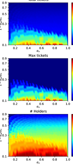
(a) Influence of threshold parameters

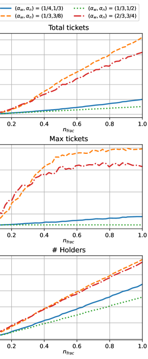
(b) Influence of the number of parties

Figure 2. Experiment results using Aptos

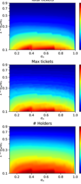
(a) Influence of threshold parameters

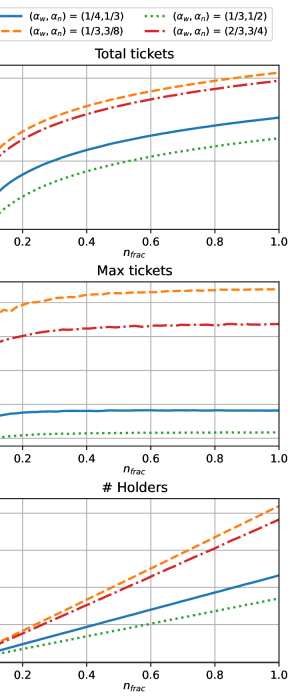
(b) Influence of the number of parties

Figure 3. Experiment results using Filecoin

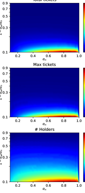
(a) Influence of threshold parameters

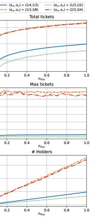
(b) Influence of the number of parties

Figure 4. Experiment results using Algorand

References

- (1)
- alg ([n. d.]) [n. d.]. Algorand stake distribution. https://algoexplorer.io/top-accounts. Accessed: 2023-03-28.
- apt ([n. d.]) [n. d.]. Aptos stake distribution. https://aptoscan.com/validators?ps=100&p=. Accessed: 2023-03-28.
- fil ([n. d.]) [n. d.]. Filecoin stake distribution. https://filfox.info/en/ranks/power. Accessed: 2023-03-28.
- tez ([n. d.]) [n. d.]. Tezos stake distribution. https://tezos.fish/leaderboard/all. Accessed: 2023-03-28.
- Abraham et al. (2021) Ittai Abraham, Philipp Jovanovic, Mary Maller, Sarah Meiklejohn, Gilad Stern, and Alin Tomescu. 2021. Reaching consensus for asynchronous distributed key generation. In Proceedings of the 2021 ACM Symposium on Principles of Distributed Computing. 363–373.
- Abraham et al. (2019) Ittai Abraham, Dahlia Malkhi, and Alexander Spiegelman. 2019. Asymptotically optimal validated asynchronous byzantine agreement. In Proceedings of the 2019 ACM Symposium on Principles of Distributed Computing. 337–346.
- Aptos (2022) Aptos. 2022. White paper – The Aptos Blockchain: Safe, Scalable, and Upgradeable Web3 Infrastructure. Technical Report. https://aptos.dev/aptos-white-paper/
- Azouvi and Vukolić (2022) Sarah Azouvi and Marko Vukolić. 2022. Pikachu: Securing PoS Blockchains from Long-Range Attacks by Checkpointing into Bitcoin PoW using Taproot. In Proceedings of the 2022 ACM Workshop on Developments in Consensus. 53–65.
- Beimel and Weinreb (2006) Amos Beimel and Enav Weinreb. 2006. Monotone circuits for monotone weighted threshold functions. Inform. Process. Lett. 97, 1 (2006), 12–18.
- Benhamouda et al. (2022) Fabrice Benhamouda, Shai Halevi, and Lev Stambler. 2022. Weighted Secret Sharing from Wiretap Channels. Cryptology ePrint Archive (2022).
- Boldyreva (2002) Alexandra Boldyreva. 2002. Threshold Signatures, Multisignatures and Blind Signatures Based on the Gap-Diffie-Hellman-Group Signature Scheme. In Public Key Cryptography — PKC 2003, Yvo G. Desmedt (Ed.). Springer Berlin Heidelberg, Berlin, Heidelberg, 31–46.
- Boneh et al. (2020a) Dan Boneh, Saba Eskandarian, Lucjan Hanzlik, and Nicola Greco. 2020a. Single secret leader election. In Proceedings of the 2nd ACM Conference on Advances in Financial Technologies. 12–24.
- Boneh et al. (2020b) Dan Boneh, Saba Eskandarian, Lucjan Hanzlik, and Nicola Greco. 2020b. Single secret leader election. In Proceedings of the 2nd ACM Conference on Advances in Financial Technologies. 12–24.
- Boneh et al. (2018) Dan Boneh, Rosario Gennaro, Steven Goldfeder, Aayush Jain, Sam Kim, Peter MR Rasmussen, and Amit Sahai. 2018. Threshold cryptosystems from threshold fully homomorphic encryption. In Advances in Cryptology–CRYPTO 2018: 38th Annual International Cryptology Conference, Santa Barbara, CA, USA, August 19–23, 2018, Proceedings, Part I 38. Springer, 565–596.
- Bracha and Toueg (1985) Gabriel Bracha and Sam Toueg. 1985. Asynchronous consensus and broadcast protocols. Journal of the ACM (JACM) 32, 4 (1985), 824–840.
- Cachin et al. (2011) Christian Cachin, Rachid Guerraoui, and Luís Rodrigues. 2011. Introduction to reliable and secure distributed programming. Springer Science & Business Media.
- Cachin et al. (2002) Christian Cachin, Klaus Kursawe, Anna Lysyanskaya, and Reto Strobl. 2002. Asynchronous verifiable secret sharing and proactive cryptosystems. In Proceedings of the 9th ACM Conference on Computer and Communications Security. 88–97.
- Cachin et al. (2001) Christian Cachin, Klaus Kursawe, Frank Petzold, and Victor Shoup. 2001. Secure and efficient asynchronous broadcast protocols. In Advances in Cryptology—CRYPTO 2001: 21st Annual International Cryptology Conference, Santa Barbara, California, USA, August 19–23, 2001 Proceedings. Springer, 524–541.
- Cachin et al. (2000) Christian Cachin, Klaus Kursawe, and Victor Shoup. 2000. Random oracles in constantipole: practical asynchronous byzantine agreement using cryptography. In Proceedings of the nineteenth annual ACM symposium on Principles of distributed computing. 123–132.
- Cachin and Tessaro (2005) Christian Cachin and Stefano Tessaro. 2005. Asynchronous verifiable information dispersal. In 24th IEEE Symposium on Reliable Distributed Systems (SRDS’05). IEEE, 191–201.
- Canetti and Rabin (1993) Ran Canetti and Tal Rabin. 1993. Fast asynchronous Byzantine agreement with optimal resilience. In Proceedings of the twenty-fifth annual ACM symposium on Theory of computing. 42–51.
- Castro et al. (1999) Miguel Castro, Barbara Liskov, et al. 1999. Practical byzantine fault tolerance. In OsDI, Vol. 99. 173–186.
- Catalano et al. (2022) Dario Catalano, Dario Fiore, and Emanuele Giunta. 2022. Adaptively secure single secret leader election from DDH. In Proceedings of the 2022 ACM Symposium on Principles of Distributed Computing. 430–439.
- Catalano et al. (2023) Dario Catalano, Dario Fiore, and Emanuele Giunta. 2023. Efficient and universally composable single secret leader election from pairings. In Public-Key Cryptography–PKC 2023: 26th IACR International Conference on Practice and Theory of Public-Key Cryptography, Atlanta, GA, USA, May 7–10, 2023, Proceedings, Part I. Springer, 471–499.
- Chaidos and Kiayias (2021) Pyrros Chaidos and Aggelos Kiayias. 2021. Mithril: Stake-based threshold multisignatures. Cryptology ePrint Archive (2021).
- Colson et al. (2007) Benoît Colson, Patrice Marcotte, and Gilles Savard. 2007. An overview of bilevel optimization. Annals of operations research 153, 1 (2007), 235–256.
- Conforti et al. (2014) Michele Conforti, Gérard Cornuéjols, Giacomo Zambelli, et al. 2014. Integer programming. Vol. 271. Springer.
- Danezis et al. (2022) George Danezis, Lefteris Kokoris-Kogias, Alberto Sonnino, and Alexander Spiegelman. 2022. Narwhal and tusk: a dag-based mempool and efficient bft consensus. In Proceedings of the Seventeenth European Conference on Computer Systems. 34–50.
- Das et al. (2023) Sourav Das, Philippe Camacho, Zhuolun Xiang, Javier Nieto, Benedikt Bunz, and Ling Ren. 2023. Threshold Signatures from Inner Product Argument: Succinct, Weighted, and Multi-threshold. Cryptology ePrint Archive (2023).
- Das et al. (2021) Sourav Das, Zhuolun Xiang, and Ling Ren. 2021. Asynchronous data dissemination and its applications. In Proceedings of the 2021 ACM SIGSAC Conference on Computer and Communications Security. 2705–2721.
- Das et al. (2022) Sourav Das, Thomas Yurek, Zhuolun Xiang, Andrew Miller, Lefteris Kokoris-Kogias, and Ling Ren. 2022. Practical asynchronous distributed key generation. In 2022 IEEE Symposium on Security and Privacy (SP). IEEE, 2518–2534.
- Desmedt (1993) Yvo Desmedt. 1993. Threshold cryptosystems. In Advances in Cryptology—AUSCRYPT’92: Workshop on the Theory and Application of Cryptographic Techniques Gold Coast, Queensland, Australia, December 13–16, 1992 Proceedings 3. Springer, 1–14.
- Dogecoin (2022) Dogecoin. 2022. White paper – Dogechain. Technical Report. https://dogechain.dog/DogechainWP.pdf
- Duan et al. (2018) Sisi Duan, Michael K Reiter, and Haibin Zhang. 2018. BEAT: Asynchronous BFT made practical. In Proceedings of the 2018 ACM SIGSAC Conference on Computer and Communications Security. 2028–2041.
- Freitas et al. (2023) Luciano Freitas, Andrei Tonkikh, Adda-Akram Bendoukha, Sara Tucci-Piergiovanni, Renaud Sirdey, Oana Stan, and Petr Kuznetsov. 2023. Homomorphic Sortition–Single Secret Leader Election for PoS Blockchains. Cryptology ePrint Archive (2023).
- Garg et al. (2022) Sanjam Garg, Abhishek Jain, Pratyay Mukherjee, Rohit Sinha, Mingyuan Wang, and Yinuo Zhang. 2022. Cryptography with Weights: MPC, Encryption and Signatures. Cryptology ePrint Archive (2022).
- Garrammone (2013) Giuliano Garrammone. 2013. On decoding complexity of reed-solomon codes on the packet erasure channel. IEEE Communications Letters 17, 4 (2013), 773–776.
- Gifford (1979) David K Gifford. 1979. Weighted voting for replicated data. In Proceedings of the seventh ACM symposium on Operating systems principles. 150–162.
- Goodman (2014) L.M Goodman. 2014. White paper – Tezos: a self-amending crypto-ledger. Technical Report. https://tezos.com/whitepaper.pdf
- Hendricks et al. (2007) James Hendricks, Gregory R Ganger, and Michael K Reiter. 2007. Verifying distributed erasure-coded data. In Proceedings of the twenty-sixth annual ACM symposium on Principles of distributed computing. 139–146.
- Ito et al. (1989) Mitsuru Ito, Akira Saito, and Takao Nishizeki. 1989. Secret sharing scheme realizing general access structure. Electronics and Communications in Japan (Part III: Fundamental Electronic Science) 72, 9 (1989), 56–64.
- Jain et al. (2017) Aayush Jain, Peter MR Rasmussen, and Amit Sahai. 2017. Threshold fully homomorphic encryption. Cryptology ePrint Archive (2017).
- Justesen (1976) Jørn Justesen. 1976. On the complexity of decoding Reed-Solomon codes (Corresp.). IEEE transactions on information theory 22, 2 (1976), 237–238.
- Keidar et al. (2021) Idit Keidar, Eleftherios Kokoris-Kogias, Oded Naor, and Alexander Spiegelman. 2021. All you need is dag. In Proceedings of the 2021 ACM Symposium on Principles of Distributed Computing. 165–175.
- Kellerer et al. (2004) H. Kellerer, U. Pferschy, and D. Pisinger. 2004. Knapsack Problems. Springer, Berlin, Germany.
- Labs (2017) Protocol Labs. 2017. White paper – Filecoin: A Decentralized Storage Network. Technical Report. https://filecoin.io/filecoin.pdf
- MacWilliams and Sloane (1977) Florence Jessie MacWilliams and Neil James Alexander Sloane. 1977. The theory of error-correcting codes. Vol. 16. Elsevier.
- Malkhi and Reiter (1997) Dahlia Malkhi and Michael Reiter. 1997. Byzantine quorum systems. In Proceedings of the twenty-ninth annual ACM symposium on Theory of computing. 569–578.
- Micali (2016) Silvio Micali. 2016. ALGORAND: The Efficient and Democratic Ledger. CoRR abs/1607.01341 (2016). arXiv:1607.01341 http://arxiv.org/abs/1607.01341
- Miller et al. (2016) Andrew Miller, Yu Xia, Kyle Croman, Elaine Shi, and Dawn Song. 2016. The honey badger of BFT protocols. In Proceedings of the 2016 ACM SIGSAC conference on computer and communications security. 31–42.
- Naor and Wool (1998) Moni Naor and Avishai Wool. 1998. The load, capacity, and availability of quorum systems. SIAM J. Comput. 27, 2 (1998), 423–447.
- Nayak et al. (2020) Kartik Nayak, Ling Ren, Elaine Shi, Nitin H Vaidya, and Zhuolun Xiang. 2020. Improved Extension Protocols for Byzantine Broadcast and Agreement. In 34th International Symposium on Distributed Computing.
- Nazirkhanova et al. (2021) Kamilla Nazirkhanova, Joachim Neu, and David Tse. 2021. Information dispersal with provable retrievability for rollups. arXiv preprint arXiv:2111.12323 (2021).
- Ohta and Okamoto (1999) Kazuo Ohta and Tatsuaki Okamoto. 1999. Multi-signature schemes secure against active insider attacks. IEICE Transactions on Fundamentals of Electronics, Communications and Computer Sciences 82, 1 (1999), 21–31.
- Rabin (1983) Michael O Rabin. 1983. Randomized byzantine generals. In 24th annual symposium on foundations of computer science (sfcs 1983). IEEE, 403–409.
- Rabin (1989) Michael O Rabin. 1989. Efficient dispersal of information for security, load balancing, and fault tolerance. Journal of the ACM (JACM) 36, 2 (1989), 335–348.
- Shamir (1979) Adi Shamir. 1979. How to share a secret. Commun. ACM 22, 11 (1979), 612–613.
- Shoup (2000) Victor Shoup. 2000. Practical threshold signatures. In Advances in Cryptology—EUROCRYPT 2000: International Conference on the Theory and Application of Cryptographic Techniques Bruges, Belgium, May 14–18, 2000 Proceedings 19. Springer, 207–220.
- Spiegelman et al. (2022) Alexander Spiegelman, Neil Giridharan, Alberto Sonnino, and Lefteris Kokoris-Kogias. 2022. Bullshark: Dag bft protocols made practical. In Proceedings of the 2022 ACM SIGSAC Conference on Computer and Communications Security. 2705–2718.
- Stinson and Strobl (2001) Douglas R. Stinson and Reto Strobl. 2001. Provably Secure Distributed Schnorr Signatures and a (t, n) Threshold Scheme for Implicit Certificates. In Proceedings of the 6th Australasian Conference on Information Security and Privacy (ACISP ’01). Springer-Verlag, Berlin, Heidelberg, 417–434.
- Yang et al. (2022) Lei Yang, Seo Jin Park, Mohammad Alizadeh, Sreeram Kannan, and David Tse. 2022. DispersedLedger: High-Throughput Byzantine Consensus on Variable Bandwidth Networks. In 19th USENIX Symposium on Networked Systems Design and Implementation (NSDI 22). 493–512.
- Yin et al. (2019) Maofan Yin, Dahlia Malkhi, Michael K Reiter, Guy Golan Gueta, and Ittai Abraham. 2019. HotStuff: BFT consensus with linearity and responsiveness. In Proceedings of the 2019 ACM Symposium on Principles of Distributed Computing. 347–356.