Steady state thermodynamics of ideal gas in shear flow

Abstract

Equilibrium thermodynamics describes the energy exchange of a body with its environment. Here, we describe the global energy exchange of an ideal gas in the Coutte flow in a thermodynamic-like manner. We derive a fundamental relation between internal energy as a function of parameters of state. We analyze a non-equilibrium transition in the system and postulate the extremum principle, which determines stable stationary states in the system. The steady-state thermodynamic framework resembles equilibrium thermodynamics.

I Introduction

There is mounting evidence that the exchange of energy of a macroscopic steady state system with its environment can be described in an equilibrium thermodynamic-like fashion. It has been considered in the 90s of the twentieth century for systems with chemical reactions that may constantly occur in time (ross1988thermodynamics, ; hunt1990thermodynamic, ; ross1992thermodynamic, ). Such a steady state situation goes beyond equilibrium thermodynamics which excludes any macroscopic flows and currents (Thermodynamics_and_an_Introduction_to_Thermostatistics_2ed_H_Callen, ). Around a similar time, the thermodynamic-like approach was introduced for systems with shear-flow (evans1980thermodynamics, ; hanley1982thermodynamics, ; evans1983computer, ; evans1986rheology, ) and is still under development (daivis2003steady, ; taniguchi2004steady, ; daivis2008thermodynamic, ; baranyai2018thermodynamic, ). Another class of macroscopic systems for which the attempt to introduce thermodynamic description has been undertaken is systems with heat flow (nakagawa2019global, ; nakagawa2022unique, ; Zhang2021continuous, ; holyst2022thermodynamics, ; Holyst2023Steady, ).

The above approaches to formulate steady state thermodynamics focus on chemical reactions and shear flow, both in homogeneous temperature profiles or systems with heat flow without chemical reactions and macroscopic flows. If steady state thermodynamics is ever formulated on general grounds, it is now at its inception. About two decades ago, Oono and Paniconi (oono1998steady, ) and Sasa and Hatano (sasa2006steady, ) postulated a thermodynamic-like description based on a general footing. However, because the descriptions were postulated, they require validation and further investigation on the eventual limitation. In particular, it is not clear whether the nonequilibrium entropy defined by the integral of the local entropy density over the volume of the system (nakagawa2022unique, ) or rather the excess heat-based entropy (oono1998steady, ) should be used to construct the principles of steady-state thermodynamics. These two entropies are not equivalent (holyst2022thermodynamics, ). It shows that the steady state thermodynamics is far from complete, and the core fundamental questions still remain open (Holyst2023Steady, ; nakagawa2022unique, ). It is worth mentioning stochastic thermodynamics, which focuses on thermodynamic notions for the system on the level of individual trajectories (seifert2012stochastic, ; ding2022unified, ). Here we focus on a reduced, macroscopic description of a steady state system (speck2021modeling, ).

Allowing various macroscopic constant fluxes drives the system from equilibrium to a steady state and opens up phenomena that eludes equilibrium thermodynamics. Take for example a quiescent liquid in a uniform gravitational field in equilibrium. This situation assumes a uniform temperature and no macroscopic flows, which, together with the equations of state, determine the thermodynamic parameters at each point of the system. Allowing a vertical or horizontal heat flow radically changes the situation. The flow of heat combined with the gravitational force can cause regular mass movement, either because the denser liquid is at the top and the thinner is at the bottom or because gravity unevenly acts on areas with different horizontal densities. This unstable situation causes a mass movement in the atmosphere, oceans, planets, and stars (bodenschatz2000recent, ). The core feature of this phenomenon is the coupling between the heat flow and the mass flow. However, the question arises whether some reduced description for non-equilibrium steady states also emerges from hydrodynamics. Can it take the shape of equilibrium thermodynamics, in which the system’s behavior is described by only a few parameters and the rules of extremum containing only these parameters?

Here we present a thermodynamic-like description of a system with heat and mass flow coupling. We consider ideal gas in shear flow with a dissipative temperature profile shown schematically in Fig. 1. We introduce the first law for this system that describes different ways of exchanging the system’s energy with its environment. We also consider a movable wall as a thermodynamic constraint in the system. We introduce the extremum principle that determines the position of the wall. We show that there is a critical shear in the system above which the equilibrium position of the internal wall becomes unstable, and the system undergoes a nonequilibrium second order phase transition. We give a complete thermodynamic-like description of this steady state system in which the position of the movable wall is a thermodynamic constraint. For the vanishing shear flow, the steady state extremum principle directly reduces to the minimum principle in the corresponding problem in thermodynamics.

II System

We consider ideal monoatomic gas between two two parallel walls at walls’ temperature $T_{0}$, as shown in Fig. 1. The upper wall moves with speed $V_{w}$ moving in $x$-direction. The system is described by irreversible thermodynamic equations: the continuity equation, Navier-Stokes equation, energy balance and two equations of state (Groot_Mazur_Non-equilibrium_thermodynamics, ). We assume that the system is translationally invariant in $x$ and $y$ directions, therefore the fields depend only on $z$ coordinate. In particular, equations of state are given by,

$$p\left(z\right)=n\left(z\right)k_{B}T\left(z\right),$$ (1)

$$u\left(z\right)=\frac{3}{2}n\left(z\right)k_{B}T\left(z\right),$$ (2)

with pressure $p\left(z\right),$ volumetric particle number density $n\left(z\right)$, temperature $T\left(z\right)$, Boltzmann constant $k_{B}$, and the volumetric energy density, $u\left(z\right)$. The velocity field also depends on $z$ coordinate only and is oriented in the direction determined by the moving wall,

$$\mathbf{v}\left(x,y,z\right)={\bf e}_{x}v\left(z\right).$$ (3)

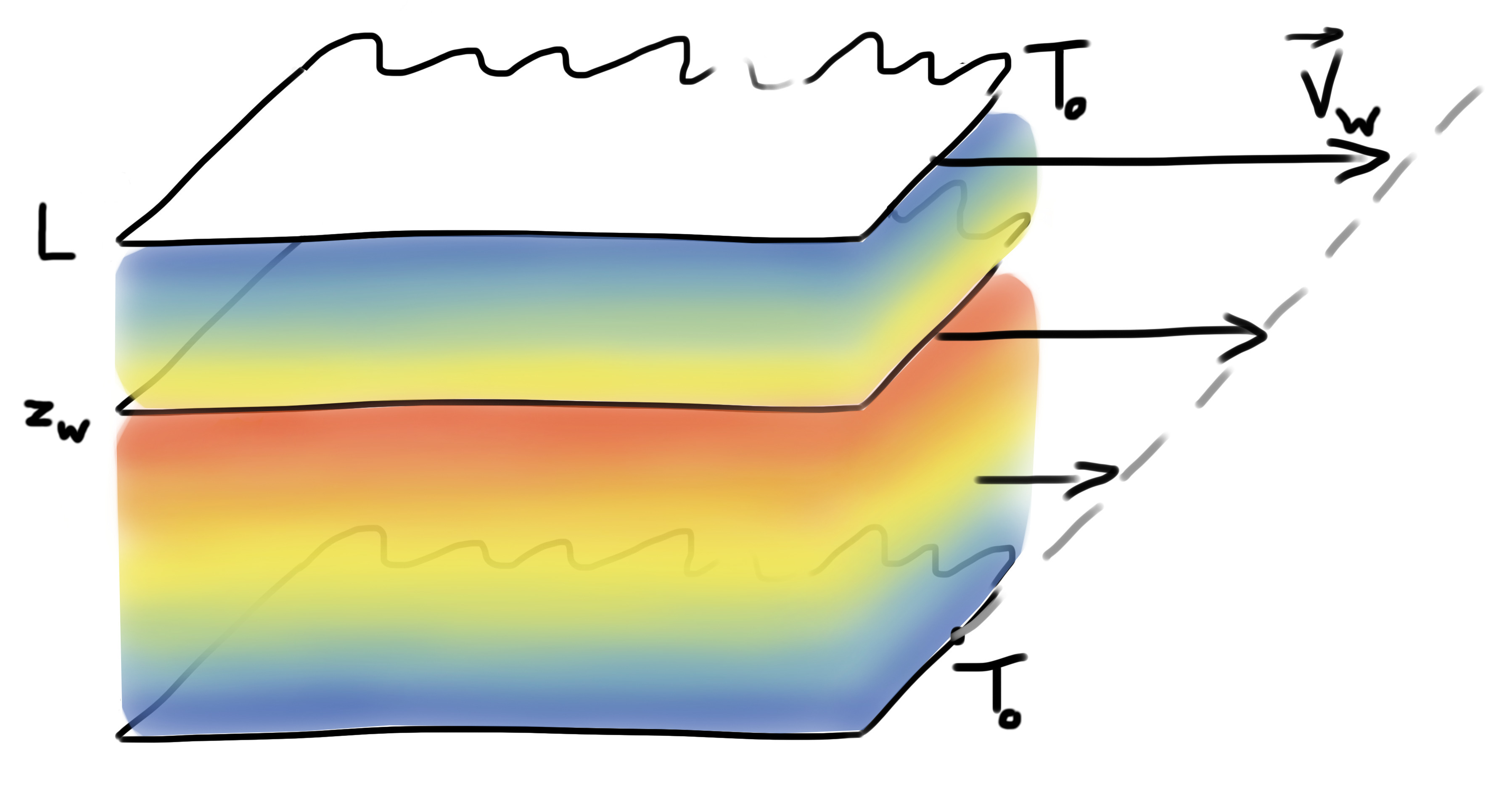
Figure 1: Ideal gas in shear flow. The gas is confined by the immobile bottom wall and by the upper wall moving with velocity $V_{w}$. There is also a thermally insulating and moving internal wall that divides the gas into two subsystems. Shearing motion causes energy dissipation in the system, which changes the temperature profile. The heat flows out from the system through the confining walls at temperature $T$. Colors schematically show the temperature profile (red - hotter, blue - colder).

III Steady state

We describe the system within linear response theory (Groot_Mazur_Non-equilibrium_thermodynamics, ). Therefore, the system is locally described by equation of states (1) and (2) supplemented with mass, momentum and energy conservation. We neglect bulk viscosity. We assume that the shear viscosity coefficient $\eta$ does not depend on the local state of the gas, so the viscosity does not depend on local density and temperature. The translational symmetry for the pressure, $p\left({\bf r}\right)=p\left(z\right)$, and for the velocity given by Eq. (3) reduces the $z$-component of the Navier-Stokes equation,

$$\rho\left(\partial_{t}{\bf v}+\left({\bf v}\cdot\nabla\right){\bf v}\right)=-\nabla p+\eta\Delta{\bf v}+\frac{1}{3}\eta\nabla\left(\nabla\cdot{\bf v}\right),$$ (4)

to the formula, $dp\left(z\right)/dz=0$, while the $x$-component of the Navier-Stokes equation gives $0=\eta d^{2}v\left(z\right)/dz^{2}$. Therefore the pressure in the system is homogeneous,

$$p\left(z\right)=p,$$ (5)

and, using the boundary conditions $v\left(0\right)=0$ and $v\left(L\right)=V_{w}$, there is a shear flow in the system,

$$v\left(z\right) =\frac{z}{L}V_{w}.$$ (6)

The continuity equation,

$$\partial_{t}\rho+{\bf v}\cdot\nabla\rho=-\rho\nabla\cdot{\bf v},$$ (7)

with mass density $\rho\left(z\right)$ and the above velocity field is satisfied automatically for any density profile. The energy balance equation is given by,

$$\rho\left(\partial_{t}u_{m}+{\bf v}\cdot\nabla u_{m}\right) =\kappa\Delta T-p\nabla\cdot{\bf v}$$

$$+2\eta\mathring{\left[\text{$\nabla$}{\bf v}\right]}^{s}:\mathring{\left[\text{$\nabla$}{\bf v}\right]}^{s},$$ (8)

where $\mathring{\left[\text{$\nabla$}{\bf v}\right]}_{ij}^{s}=\left(\nabla_{i}\mathbf{v}_{j}+\nabla_{j}\mathbf{v}_{i}-\delta_{ij}\frac{2}{3}\nabla\cdot{\bf v}\right)/2$ denotes the symmetrized and traceless velocity gradient matrix, the colon is the double contraction, $\delta_{ij}$ denotes the Kronecker delta, and $u_{m}=u/\rho$ is the mass density of the internal energy. Utilizing the shear velocity profile (6) and the translational invariance of the internal energy density, $u_{m}\left(z\right)$, the energy balance equation reduces to the equation for the temperature profile

$$0=\kappa\frac{d^{2}}{dz^{2}}T\left(z\right)+\eta\left(\frac{V_{w}}{L}\right)^{2}.$$ (9)

The above equation has the following form, $0=\kappa\frac{d^{2}}{dz^{2}}T\left(z\right)+\lambda$, where $\lambda$ is the volumetric heating rate,

$$\lambda=\eta\left(\frac{V_{w}}{L}\right)^{2}.$$ (10)

We also introduce the dimensionless parameter

$$D\equiv\frac{\eta V_{w}^{2}}{\kappa T_{0}}.$$

IV Shear flow without the internal wall

We first consider the shear flowing system shown in Fig. 1, but without the internal wall. In this situation, the boundary conditions are that on the upper and lower surface and the temperature profile is given by,

$$T\left(z\right)=T_{0}\left[-\frac{1}{2}\frac{\lambda L^{2}}{\kappa T_{0}}\left(\frac{z}{L}\right)^{2}+\frac{1}{2}\frac{\lambda L^{2}}{\kappa T_{0}}\frac{z}{L}+1\right].$$ (11)

Number of particles in the surface area $A$ of the translationally invariant system is determined by the particle density, $N=A\int_{0}^{L}dz\,n\left(z\right)$, which with the mechanical equation of state (1) and the above temperature profile gives

$$p=\frac{Nk_{B}T_{0}}{AL}\psi\left(\frac{\eta V_{w}^{2}}{\kappa T_{0}}\right),$$ (12)

where

$$\psi(D)\equiv\frac{D}{8\sqrt{\frac{D}{8+D}}\tanh^{-1}\sqrt{\frac{D}{8+D}}}.$$ (13)

Combination of equations of state (1) and (2) gives the following internal energy density $u\left(z\right)=3p\left(z\right)/2.$ Total internal energy in the system is given by

$$U=A\int_{0}^{L}dz\,u\left(z\right)=\frac{3}{2}ALp,$$ (14)

where we used the fact, that the pressure in the system is constant. Utilizing Eq. (12) in the above equation we get,

$$U=\frac{3}{2}Nk_{B}T_{0}\psi\left(\frac{\eta V_{w}^{2}}{\kappa T_{0}}\right).$$ (15)

We determine the kinetic energy due to macroscopic motion, $E_{k}=A\int_{0}^{L}dz\,mn\left(z\right)v^{2}\left(z\right)/2,$ where $m$ is a mass of a single ideal gas molecule. We obtain

$$E_{k}=mN\frac{V_{w}^{2}}{2}\varepsilon\left(\frac{\eta V_{w}^{2}}{\kappa T_{0}}\right),$$ (16)

where

$$\varepsilon\left(D\right)=\frac{2}{D}\left(\frac{4+D}{4}\frac{1}{\psi\left(D\right)}-1\right).$$ (17)

Utilizing Eqs. (15), (16) and (17) we obtain the relation between the kinetic and internal energy,

$$E_{k}\frac{\eta}{mN\kappa T_{0}}=\frac{4+\frac{\eta V_{w}^{2}}{\kappa T_{0}}}{4}\frac{\frac{3}{2}Nk_{B}T_{0}}{U}-1.$$ (18)

V Transition between steady states and energy balance

We consider transitions between steady states in the system. The system is in one steady state at time $t_{i}$ , after which we slightly change one or more control parameters that appear in (or are related to) the governing equations. For example, we slowly modify the velocity of the wall, the position of the upper wall (volume $V$) or the external temperature $T_{0}$. In particular, we increase the velocity of the wall by $V_{w}\left(t\right)=V_{w}+\left(t-t_{i}\right)dV_{w}/\left(t_{f}-t_{i}\right)$ for $t_{i}<t<t_{f}$, which modifies velocity of the wall from $V_{w}$ to $V_{w}+dV_{w}$. This induces a time dependent hydrodynamic field. After time $t_{f}$ the system reaches another steady state close to the previous one due to a small change in the control parameters. We focus on steady, nonequilibrium states with a constant number of particles in the system.

Previously we have analyzed the energy balance for an ideal gas in a heat flow (holyst2022thermodynamics, ) during the transition between steady states. The considerations necessary for Couette flow go along the same line. We do not repeat them but give a sketch. We monitor the change of the energy between times $t_{i}$ and $t_{f}$,

$$dU=U\left(t_{f}\right)-U\left(t_{i}\right)=\int_{t_{i}}^{t_{f}}dt\,\frac{dU\left(t\right)}{dt},$$

where

$$U\left(t\right)=\int_{V(t)}d^{3}r\,\rho\left({\bf r},t\right)u\left({\bf r},t\right),$$ (19)

and $\rho\left({\bf r},t\right)$ is the density and $u\left({\bf r},t\right)$ is the internal energy density per unit mass at position ${\bf r}$ and time $t$. We then represent the time derivative of the above integral utilizing the internal energy balance equation (8). Applying analysis from (holyst2022thermodynamics, ) leads to the conclusion that the system exchanges the energy with the environment according to the following formula,

$$dU=\mkern 3.0mu\mathchar 22\relax\mkern-12.0mudQ+\mkern 3.0mu\mathchar 22\relax\mkern-12.0mudW+\mkern 3.0mu\mathchar 22\relax\mkern-12.0mudD,$$ (20)

with the excess heat defined by

$$\mkern 3.0mu\mathchar 22\relax\mkern-12.0mudQ=-\int_{t_{i}}^{t_{f}}dt\int_{\partial V\left(t\right)}d^{2}r\,\hat{n}\cdot\left(J_{q}\left(t\right)-J_{q,st}\left(t\right)\right),$$ (21)

where $\hat{n}$ is the vector normal to the surface of volume $V$ and $J_{q}\left(t\right)$ is the heat flux in the system, with the work related to the expansion of the gas defined by

$$\mkern 3.0mu\mathchar 22\relax\mkern-12.0mudW=-\int_{t_{i}}^{t_{f}}dt\int_{V\left(t\right)}d^{3}r\,p\nabla\cdot{\bf v},$$ (22)

and the excess dissipation defined by,

$$\mkern 3.0mu\mathchar 22\relax\mkern-12.0mudD=\int_{t_{i}}^{t_{f}}dt\int_{V\left(t\right)}d^{3}r\,\left(\Pi:\left[\nabla{\bf v}\right]-\Pi_{st}\left(t\right):\left[\nabla{\bf v}_{st}\left(t\right)\right]\right),$$ (23)

where $\left[\nabla{\bf v}\right]_{ij}=\nabla_{i}{\bf v}_{j}$ is the gradient velocity matrix. The subscript $st$ in the above equations means that the quantity should be taken at a stationary state that corresponds to the control parameters at time $t$. The first term in the internal energy balance (20), $\mkern 3.0mu\mathchar 22\relax\mkern-12.0mudQ$, is the heat on top of the steady state heat exchanged during the transition between steady states (oono1998steady, ). The second term in (20) is the volumetric work performed by that wall (more specifically, by the perpendicular component of the force of the wall) when the system is compressed. The third term $\mkern 3.0mu\mathchar 22\relax\mkern-12.0mudD$ is the energy dissipation in the system on top of the steady state dissipation.

Because the pressure in a steady state is spatially uniform, the work from Eq. (22) for slow transitions between steady states reduces as follows, $\mkern 3.0mu\mathchar 22\relax\mkern-12.0mudW\approx-p\int_{t_{i}}^{t_{f}}dt\int_{V\left(t\right)}d^{3}r\,\nabla\cdot{\bf v}$. The integrals of the divergence with the Gauss theorem reduce to the change of the volume, and the work reduces to the volumetric work that also appears in equilibrium thermodynamics,

$$\mkern 3.0mu\mathchar 22\relax\mkern-12.0mudW=-pdV.$$

To determine the exchange of the kinetic energy, we proceed along the same line as for the internal energy above. Thus we use the kinetic energy balance equation (Groot_Mazur_Non-equilibrium_thermodynamics, ),

$$\partial_{t}\frac{1}{2}\rho{\bf v}^{2}=-\nabla\cdot\left(\frac{1}{2}\rho{\bf v}^{2}{\bf v}+P\cdot{\bf v}\right)+P:\left[\nabla{\bf v}\right],$$ (24)

where the pressure tensor $P$ in the system is given by

$$P_{ij} =p\delta_{ij}+\Pi_{ij},$$

$$\Pi =-2\eta\mathring{\left[\text{$\nabla$}{\bf v}\right]}^{s}.$$

Analysis of the change of the kinetic energy $dE_{k}=E_{k}\left(t_{f}\right)-E_{k}\left(t_{i}\right)=\int_{t_{i}}^{t_{f}}dt\,\frac{dE_{k}\left(t\right)}{dt}$ leads to the conclusion that during the transition between steady states, the kinetic energy changes according to the following equation,

$$dE_{k}=\mkern 3.0mu\mathchar 22\relax\mkern-12.0mudW_{w}-\mkern 3.0mu\mathchar 22\relax\mkern-12.0mudD,$$ (25)

where

$$\mkern 3.0mu\mathchar 22\relax\mkern-12.0mudW_{w}=\int_{t_{i}}^{t_{f}}dt\int_{\partial V\left(t\right)}d^{2}r\,\hat{n}\cdot\left(\Pi\cdot{\bf v}-\Pi_{st}\left(t\right)\cdot{\bf v}_{st}\left(t\right)\right)$$

According to the above equations, the kinetic energy may change in two ways. $\mkern 3.0mu\mathchar 22\relax\mkern-12.0mudW_{w}$ is the work performed by the upper wall on top of the steady work performed to keep the shearing steady state. It may be called the excess shear work of the wall. This effect has been recently discussed by Baranyai (baranyai2018thermodynamic, ).

The differential of the total energy, $E=U+E_{k}$ follows from Eqs. (20) and (25) and is given by,

$$dE=\mkern 3.0mu\mathchar 22\relax\mkern-12.0mudQ-pdV+\mkern 3.0mu\mathchar 22\relax\mkern-12.0mudW_{w}.$$ (26)

The total energy changes as a result of the excess heat $\mkern 3.0mu\mathchar 22\relax\mkern-12.0mudQ$, volumetric work $-pdV$, and the excess shear work $\mkern 3.0mu\mathchar 22\relax\mkern-12.0mudW_{w}$. Contrary to the energy balance equations (20) and (25), there is no excess dissipation $\mkern 3.0mu\mathchar 22\relax\mkern-12.0mudD$ defined by Eq. (23) in the above total energy balance equation. It follows that the excess dissipation $\mkern 3.0mu\mathchar 22\relax\mkern-12.0mudD$ describes an internal transfer of internal and kinetic energy. During the steady state transition, part of the kinetic energy changes to internal energy through the kinetic energy dissipation that occurs on top of the steady state dissipation.

VI Nonequilibrium entropy

By introducing

$$\mkern 3.0mu\mathchar 22\relax\mkern-12.0mudP\equiv\mkern 3.0mu\mathchar 22\relax\mkern-12.0mudQ+\mkern 3.0mu\mathchar 22\relax\mkern-12.0mudD$$ (27)

we obtain the internal energy balance (20) in the following form,

$$dU=\mkern 3.0mu\mathchar 22\relax\mkern-12.0mudP-pdV.$$ (28)

The above formula holds in the space of the control parameters, which are temperature $T$, the volume of the system $V$, and the speed of the moving wall $V_{w}$. We do not change the number of particles $N$. The above formula has the same form as the internal energy of ideal gas without the macroscopic kinetic energy but with volumetric heating (holyst2022thermodynamics, ; Zhang2021continuous, ). Because the pressure in a shear flow system is constant, Eq. (5), and due to the ideal gas mechanical equation of state, Eq. (14), we obtain,

$$p=\frac{2}{3}\frac{U}{V}.$$ (29)

We notice the following two facts. First, the internal energy balance in the transition between steady states given by Eq. (28) is very similar to the equilibrium thermodynamics expression $dU_{eq}=\mkern 3.0mu\mathchar 22\relax\mkern-12.0mudQ_{eq}-pdV$. We see that the differential $\mkern 3.0mu\mathchar 22\relax\mkern-12.0mudP$ plays the role of the heat differential in equilibrium thermodynamics. Second, the expression for pressure (29) is also the equilibrium ideal gas pressure mechanical equation, $p=2U_{eq}/3V.$ The above two similarities between steady state and the equilibrium thermodynamic differentials suggest that there exists the integrating factor for $\mkern 3.0mu\mathchar 22\relax\mkern-12.0mudP$ differential,

$$\mkern 3.0mu\mathchar 22\relax\mkern-12.0mudP=T^{*}dS^{*},$$ (30)

where nonequilibrium (effective) entropy is given by the following fundamental equation for the internal energy,

$$S^{*}\left(U,V\right)=Nk_{B}\log\left[\frac{V}{N}\left(\frac{U}{N}\right)^{3/2}\right]+Ns_{0},$$ (31)

while the nonequilibrium temperature

$$T^{*}=\frac{\partial U\left(S^{*},V\right)}{\partial S^{*}}.$$ (32)

The pressure is determined by $p=-\partial U\left(S^{*},V\right)/\partial V$. Whether the differential $\mkern 3.0mu\mathchar 22\relax\mkern-12.0mudP$ has integrating factor (is exact) can also be shown directly by proving that the differential $\mkern 3.0mu\mathchar 22\relax\mkern-12.0mudP=dU/T^{*}\left(U,V,V_{w}\right)+p\left(U,V,V_{w}\right)/T^{*}\left(U,V,V_{w}\right)dV+0\cdot dV_{w}$ has equal derivatives, $\partial\left(1/T^{*}\right)/\partial V=\partial\left(p/T^{*}\right)/\partial U$ and that the differential does not explicitly depend on $V_{w}$ (Spivak_M_Calculus_on_manifolds, ).

VII System with internal wall

Now we focus on the system with the internal wall shown in Fig. 1. The wall splits the system into two parts, upper 1 and lower 2. In a steady state, the velocity field in the system is the shear flow given by Eq. (6). Therefore the velocity of the internal wall is $V_{w}^{s}=V_{w}z_{w}/L$, where $z_{w}$ is the position of this wall. The wall is adiabatically insulating, which changes one of the boundary conditions. There is no heat flow through the wall. Without the wall the temperature profile would be given by the symmetric parabola, Eq. (11), but the insertion of the adiabatic wall in the middle of the system leads to the situation with half of the parabolic profile. Using this observation, we conclude that from the perspective of the heat flow equation, we can use the solution without the internal wall to determine the energy of subsystem $2$ as follows, $U_{2}\left(T,A,L_{2},V_{w,2}^{u}\right)=U\left(T,A,2L_{2},2V_{w,2}^{u}\right)/2$, where $V_{w,2}^{u}$ is the speed of the upper wall in subsystem 2 and $L_{2}$ is the vertical length of the subsystem. Because the change to the moving reference frame does not change the internal energy, we can deduce the internal energy of the upper system in a similar manner. The internal energy in both subsystems is given by,

$$U_{i}\left(T,A,L_{i},V_{w,i}^{u}-V_{w,i}^{l}\right)$$

$$=\frac{1}{2}U\left(T,A,2L_{i},2\left(V_{w,i}^{u}-V_{w,i}^{l}\right)\right)\text{ for }i=1,2,$$

where $V_{w,i}^{u}$ is the speed of the upper wall in subsystem $i$, and $V_{w,i}^{l}$ is the speed of the lower wall in subsystem $i$. We have $V_{w,2}^{l}=0$ and $V_{w,2}^{u}=V_{w,1}^{l}$.

Using the properties of the equations of state for ideal gas we can show that the differentials

$$\mkern 3.0mu\mathchar 22\relax\mkern-12.0mudP_{i}\equiv dU_{i}^{int}+p_{i}dV_{i}\text{ for }i=1,2,$$ (33)

have integrating factors in agreement with Eq. (30),

$$\mkern 3.0mu\mathchar 22\relax\mkern-12.0mudP_{i}=T_{i}^{*}dS_{i}^{*}\text{ for }i=1,2.$$ (34)

On the other hand, the analysis of the energy balance similar to the one presented in the previous section leads to the conclusion that $\mkern 3.0mu\mathchar 22\relax\mkern-12.0mudP_{1/2}=\mkern 3.0mu\mathchar 22\relax\mkern-12.0mudQ_{1/2}+\mkern 3.0mu\mathchar 22\relax\mkern-12.0mudD_{1/2}$ is the sum of excess heat and excess dissipation in each subsystem. The differentials $\mkern 3.0mu\mathchar 22\relax\mkern-12.0mudQ_{1/2}$ and $\mkern 3.0mu\mathchar 22\relax\mkern-12.0mudD_{1/2}$ are determined by a direct application of formulas (21) and (23) with the replacement of the volume of integration with the volume for a particular subsystem.

Until now, we have discussed the energy balance independently for each subsystem. But it is particularly interesting to consider a perpendicular motion of the internal wall. As follows from the dynamics, the normal component of the pressure tensor on the wall in a steady state comes solely from hydrostatic pressure. The wall may move vertically only due to the pressure difference, $p_{1}\neq p_{2}.$ It’s natural position is where these pressures are balanced. Therefore the knowledge of the effective entropy $S^{*}$ and volume for each subsystem is sufficient to determine the force acting on the wall. The wall’s horizontal velocity enters the problem indirectly. The shear velocity plays the role of energy dissipation. The speed of the wall appears in the energy balance equation (9) in the source term. It thus plays the role of volumetric heating, $\lambda\equiv\eta\left(V_{w}/L\right)^{2}$.

The ideal gas with volumetric heating and an internal wall has already been considered previously (Zhang2021continuous, ). Such a system exhibits continuous nonequilibrium phase transition. Similarly, the system with macroscopic kinetic energy shown in Fig. 1 will exhibit the phase transition as well for the following reason. Let’s focus on the position of the internal wall $z_{w}$ and upper wall velocity, $V_{w,2}^{u}$, keeping the external walls temperature $T$, the total volume of the system, $L_{1}+L_{2}=L$, and other parameters constant. Number of particles in both subsystems is equal, $N_{1}=N_{2}$. Because the hydrostatic pressure gives the sole force normal to the walls, the motion of the internal wall can be determined by the fundamental relations (31) for each subsystem. The pressure follows from $p_{i}=p_{i}\left(U_{i},V_{i},N_{i}\right)$. Moreover, the internal energy in steady state is determined by Eq. (15). The equivalence is explicit after comparing Eq. (15) to the expression (5) from the reference (Zhang2021continuous, ). This reasoning leads to the conclusion that from the perspective of the position of the internal wall, the steady state behavior of both subsystems is the same. The speed of the upper wall for the system with kinetic energy must be related to the volumetric heating $\lambda$ from (Zhang2021continuous, ) by $\lambda\equiv\eta\left(V_{w}/L\right)^{2}$.

Because there is one-to-one correspondence, we conclude that once the upper wall’s speed increases, the shear flow volumetrically heats the system. For the value, $\lambda L^{2}/4\kappa T\approx 4.55344$, equivalently $\eta V_{w}^{2}/4\kappa T_{0}\approx 4.55344$, the central position of the wall ceases to be stable. Above the critical speed, the wall spontaneously chooses one of the two stable positions and moves away from the center.

As we show below, it is possible to introduce an extremum principle that determines the spontaneous position of the internal wall. Let’s consider an additional external force $F_{w}$ perpendicular to the wall. In a steady state it is determined by the pressure difference, $F_{ext}=-A\left(p_{2}-p_{1}\right)$. The force performs work on the system, $\mkern 3.0mu\mathchar 22\relax\mkern-12.0mudW_{ext}=-A\left(p_{2}-p_{1}\right)\,dz_{w}.$ Because the spontaneous direction of the wall is toward the equilibration of pressures, the system reaches “equilibrium” for the position of the wall $x$, for which the work done by the external force is negative,

$$\mkern 3.0mu\mathchar 22\relax\mkern-12.0mudW_{ext}<0.$$ (35)

The above phenomenological fact we use to construct the thermodynamic-like extremum principle. When the upper wall does not move vertically, the work of the external force is related to the volumetric work in both subsystems,

$$\mkern 3.0mu\mathchar 22\relax\mkern-12.0mudW_{ext}=-p_{1}dV_{1}-p_{2}dV_{2}.$$ (36)

This equation, by utilizing the internal energy balance given by Eqs. (33) and the nonequilibrium entropy, is expressed as follows,

$$\mkern 3.0mu\mathchar 22\relax\mkern-12.0mudW_{ext}=dU_{1}-T_{1}^{*}dS_{1}^{*}+dU_{2}-T_{2}^{*}dS_{2}^{*}.$$ (37)

Equivalently, it is given by

$$\mkern 3.0mu\mathchar 22\relax\mkern-12.0mudW_{ext}=dU_{12}-\mkern 3.0mu\mathchar 22\relax\mkern-12.0mudP_{12},$$ (38)

where

$$dU_{12}=dU_{1}+dU_{2}$$ (39)

and

$$\mkern 3.0mu\mathchar 22\relax\mkern-12.0mudP_{12}=\mkern 3.0mu\mathchar 22\relax\mkern-12.0mudP_{1}+\mkern 3.0mu\mathchar 22\relax\mkern-12.0mudP_{2}.$$ (40)

Eq. (38) puts us in the same position as in equilibrium thermodynamics: if $\mkern 3.0mu\mathchar 22\relax\mkern-12.0mudP_{12}$ has an integrating factor and the corresponding potential, $\mkern 3.0mu\mathchar 22\relax\mkern-12.0mudP_{12}=T_{12}^{*}dS_{12}^{*}$, then the condition of minimal work (35) by means of expression (38) follows the condition of the minimum of the energy for ‘adiabatically insulated’ system defined by $S_{12}^{*}=const$ surface. This surface is considered in the space of $T_{0},V_{1},V_{2},V_{w}$, because we keep the number of particles , $N_{1},N_{2}$, and other parameters constant. Let’s notice that expressions (35-40) for the case of no shear flow (no heating), $V_{w}=0$, reduces to the problem of finding the position of the wall that separates two homogeneous ideal gases. Thus, in equilibrium thermodynamics, $\mkern 3.0mu\mathchar 22\relax\mkern-12.0mudP$, becomes the role the heat differential. The nonequilibrium situation has been discussed earlier (holyst2022thermodynamics, ) and it suggests the minimum principle as follows.

The position of the wall is determined by the minimum of total internal energy, $U_{12},$ as a function of parameters of states $S_{1}^{*},V_{1},S_{2}^{*},V_{2},$ for the constraint

$$S_{12}^{*}=S_{1}^{*}+rS_{2}^{*}.$$ (41)

The latter condition denotes steady ‘adiabatic insulation’. In this principle there appears parameter $r$. Let’s apply the above principle to verify whether it gives a proper position of the wall and to find the meaning of $r$ parameter. We apply the above principle with the constraint of total volume of the system fixed,

$$V=V_{1}+V_{2}.$$ (42)

The total energy is given by

$$U\left(S_{1}^{*},V_{1},S_{2}^{*},V_{2}\right)=U\left(S_{1}^{*},V_{1}\right)+U\left(S_{2}^{*},V_{2}\right),$$ (43)

where $U\left(S_{1}^{*},V_{1}\right)$ follows from the fundamental relation (31). Minimization of the above energy with constraints (41) and (42) allows us to use $S_{1}^{*}$ and $V_{1}$ as two independent parameters and minimize the function $U\left(S_{1}^{*},V_{1}\right)+U\left(\left(S_{12}^{*}-S_{1}^{*}\right)/r,V-V_{1}\right)$. Its first derivatives lead to the following necessary conditions for the minimum of the function,

$$T_{1}^{*}-\frac{1}{r}T_{2}^{*} =0,$$ (44)

$$p_{1}-p_{2} =0.$$

It proves that the necessary condition for the minimum in the presented extremum principle leads to equality of pressures. The first of the above equations gives the interpretation of $r$ parameter. It is the nonequilibrium temperature ratio. Notice that when $r=1$, the entropy becomes additive (Eq. (41)) and the minimum principle reduces directly to the equilibrium minimum principle.

In the above reasoning the minimum principle follows from the fact, that the internal energy balance is determined by $dU_{i}=\mkern 3.0mu\mathchar 22\relax\mkern-12.0mudP_{i}-p_{i}dV_{i}$ with homogeneous pressure that is solely determined by the internal energy and volume, $p_{i}=p_{i}\left(U_{i},V_{i}\right)$. Both assumptions also hold when transport coefficients depend on parameters of states (Holyst2023Steady, ). In particular, if the viscosity or heat conductivity depends on density or temperature. For this reason, the derived minimum energy principle is also valid beyond the regime of Onsager’s linear response theory (Groot_Mazur_Non-equilibrium_thermodynamics, ).

It is also worth noting that the inequality (35) which determines the direction of spontaneous motion of the wall, with the use of Eq. (36) and Eq. (26) applied to each subsystem is expressed by

$$\mkern 3.0mu\mathchar 22\relax\mkern-12.0mudW_{ext}=dE_{12}-\mkern 3.0mu\mathchar 22\relax\mkern-12.0mudQ_{12}-\mkern 3.0mu\mathchar 22\relax\mkern-12.0mudW_{w12},$$

with energy differential, $dE_{12}=dE_{1}+dE_{2}$, excess heat $\mkern 3.0mu\mathchar 22\relax\mkern-12.0mudQ_{12}=\mkern 3.0mu\mathchar 22\relax\mkern-12.0mudQ_{1}+\mkern 3.0mu\mathchar 22\relax\mkern-12.0mudQ_{2}$ and excess work performed by wall, $\mkern 3.0mu\mathchar 22\relax\mkern-12.0mudW_{w12}=\mkern 3.0mu\mathchar 22\relax\mkern-12.0mudW_{w1}+\mkern 3.0mu\mathchar 22\relax\mkern-12.0mudW_{w2}$. The above formula suggests an approach to identify the quantity that is minimized in the system by subtraction from total energy all other terms (apart from work related to the change of the constraint) that are present in the energy balance equation (here, excess work performed by the wall and heat) which describe the ways the system exchanges energy with the environment. Such a way could lead to a mnemotechnic rule to identify the physical quantity to generalize the second law in other situations than considered in this paper (e.g., with the exchange of particles).

VIII Summary

In this article, we investigate whether there is a description similar to equilibrium thermodynamics for out-of-equilibrium steady states. We consider this problem in the context of the Couette flow, where there is a mass current (velocity field), energy dissipation, and a continuous flow of heat. Each feature independently excludes the theory of equilibrium thermodynamics and its tools.

Since, in general, it is still unclear that such a simple, equilibrium thermodynamic-like description of nonequilibrium steady states is possible, we have chosen the most straightforward possible system, which we believe includes the coupling of mass flow and heat current, i.e., an ideal gas in shear flow. We show that nonequilibrium entropy exists, which describes how the system gains energy through excess heat or dissipation. In addition, the nonequilibrium entropy allows us to construct the principle of minimum energy, which leads to the proper state of the system after removing the constraint, which is the force acting on the wall in the system. It proves the existence of a description of a system with an out-of-equilibrium heat and mass flow, which practically takes the form of equilibrium thermodynamics and reduces to the principle of minimum energy in equilibrium thermodynamics when the shear flow disappears.

The thermodynamic-like description introduced in this paper leads to further questions inspired by equilibrium thermodynamics. Particularly interesting are the procedures for measuring non-equilibrium state parameters, effective temperature and entropy, and measuring excess heat, dissipation, and work the wall performs. It is worth noting that the obtained result goes along the line of recent experiments of Yamamoto et al., who extended calorimetry for the measurements of the excess heat of sheared fluids (yamamoto2023calorimetry, ). Another issue is the possibility of developing the description of interacting systems, where the fundamental relationship for van der Waals gas with heat flow can be introduced. It is also interesting to ask about Maxwell’s identities, which in equilibrium thermodynamics appear very practical. Finally, it is fascinating to check whether such a description exists for other systems with coupled heat flow and mass current in the atmosphere and the chemical industry.

References

- [1] John Ross, Katharine LC Hunt, and Paul M Hunt. Thermodynamics far from equilibrium: Reactions with multiple stationary states. The Journal of chemical physics, 88(4):2719–2729, 1988.
- [2] Paul M Hunt, Katharine LC Hunt, and John Ross. Thermodynamic and stochastic theory for nonequilibrium systems with more than one reactive intermediate: Nonautocatalytic or equilibrating systems. The Journal of chemical physics, 92(4):2572–2581, 1990.
- [3] John Ross, Katharine LC Hunt, and Paul M Hunt. Thermodynamic and stochastic theory for nonequilibrium systems with multiple reactive intermediates: The concept and role of excess work. The Journal of chemical physics, 96(1):618–629, 1992.
- [4] Herbert B Callen. Thermodynamics and an Introduction to Thermostatistics. John Wiley & Sons, 2006.
- [5] Denis J Evans and HJM Hanley. A thermodynamics of steady homogeneous shear flow. Physics Letters A, 80(2-3):175–177, 1980.
- [6] HJM Hanley and Denis J Evans. A thermodynamics for a system under shear. The Journal of Chemical Physics, 76(6):3225–3232, 1982.
- [7] Denis J Evans. Computer "experiment" for nonlinear thermodynamics of couette flow. The Journal of Chemical Physics, 78(6):3297–3302, 1983.
- [8] Denis J Evans. Rheology and thermodynamics from nonequilibrium molecular dynamics. International Journal of Thermophysics, 7:573–584, 1986.
- [9] PJ Daivis and ML Matin. Steady-state thermodynamics of shearing linear viscoelastic fluids. The Journal of chemical physics, 118(24):11111–11119, 2003.
- [10] Tooru Taniguchi and Gary P Morriss. Steady shear flow thermodynamics based on a canonical distribution approach. Physical Review E, 70(5):056124, 2004.
- [11] Peter J Daivis. Thermodynamic relationships for shearing linear viscoelastic fluids. Journal of non-newtonian fluid mechanics, 152(1-3):120–128, 2008.
- [12] András Baranyai. Thermodynamic integration for the determination of nonequilibrium entropy. Journal of Molecular Liquids, 266:472–477, 2018.
- [13] Naoko Nakagawa and Shin-ichi Sasa. Global thermodynamics for heat conduction systems. Journal of Statistical Physics, 177(5):825–888, 2019.
- [14] Naoko Nakagawa and Shin-ichi Sasa. Unique extension of the maximum entropy principle to phase coexistence in heat conduction. Physical Review Research, 4(3):033155, 2022.
- [15] Yirui Zhang, Marek Litniewski, Karol Makuch, Paweł J. Żuk, Anna Maciołek, and Robert Hołyst. Continuous nonequilibrium transition driven by heat flow. Phys. Rev. E, 104:024102, Aug 2021.
- [16] Robert Hołyst, Karol Makuch, Anna Maciołek, and Paweł J Żuk. Thermodynamics of stationary states of the ideal gas in a heat flow. The Journal of Chemical Physics, 157(19):194108, 2022.
- [17] Robert Holyst, Karol Makuch, Anna Maciolek, Konrad Gizynski, and Pawel J Zuk. Steady thermodynamic fundamental relation for the interacting system in a heat flow. arXiv:2301.12732, 2023.
- [18] Yoshitsugu Oono and Marco Paniconi. Steady state thermodynamics. Progress of Theoretical Physics Supplement, 130:29–44, 1998.
- [19] Shin-ichi Sasa and Hal Tasaki. Steady state thermodynamics. Journal of statistical physics, 125(1):125–224, 2006.
- [20] Udo Seifert. Stochastic thermodynamics, fluctuation theorems and molecular machines. Reports on progress in physics, 75(12):126001, 2012.
- [21] Mingnan Ding, Fei Liu, and Xiangjun Xing. Unified theory of thermodynamics and stochastic thermodynamics for nonlinear langevin systems driven by non-conservative forces. Physical Review Research, 4(4):043125, 2022.
- [22] Thomas Speck. Modeling of biomolecular machines in non-equilibrium steady states. The Journal of Chemical Physics, 155(23):230901, 2021.
- [23] Eberhard Bodenschatz, Werner Pesch, and Guenter Ahlers. Recent developments in rayleigh-bénard convection. Annual review of fluid mechanics, 32(1):709–778, 2000.
- [24] Sybren Ruurds De Groot and Peter Mazur. Non-equilibrium thermodynamics. Courier Corporation, 2013.
- [25] Michael Spivak. Calculus on manifolds: a modern approach to classical theorems of advanced calculus. CRC press, 2018.
- [26] Taro Yamamoto, Yuki Nagae, Tomonari Wakabayashi, Tadashi Kamiyama, and Hal Suzuki. Calorimetry of phase transitions in liquid crystal 8cb under shear flow. Soft Matter, 19(8):1492–1498, 2023.