Worrisome Properties of Neural Network Controllers
and Their Symbolic Representations

Abstract

We raise concerns about controllers’ robustness in simple reinforcement learning benchmark problems. We focus on neural network controllers and their low neuron and symbolic abstractions. A typical controller reaching high mean return values still generates an abundance of persistent low-return solutions, which is a highly undesirable property, easily exploitable by an adversary. We find that the simpler controllers admit more persistent bad solutions. We provide an algorithm for a systematic robustness study and prove existence of persistent solutions and, in some cases, periodic orbits, using a computer-assisted proof methodology.

1 Introduction

The study of neural network (NN) robustness properties has a long history in the research on artificial intelligence (AI). Since establishing the existence of so-called adversarial examples in deep NNs in [14], it is well known that NN can output unexpected results by slightly perturbing the inputs and hence can be exploited by an adversary. Since then, the robustness of other NN architectures has been studied [44]. In the context of control design using reinforcement learning (RL), the robustness of NN controllers has been studied from the adversarial viewpoint [29, 42]. Due to limited interpretability and transparency, deep NN controllers are not suitable for deployment for critical applications. Practitioners prefer abstractions of deep NN controllers that are simpler and human-interpretable. Several classes of deep NN abstractions exist, including single layer or linear nets, programs, tree-like structures, and symbolic formulas. It is hoped that such abstractions maintain or improve a few key features: generalizability – the ability of the controller to achieve high performance in similar setups (e.g., slightly modified native simulator used in training); deployability – deployment of the controller in the physical world on a machine, e.g., an exact dynamical model is not specified and the time horizon becomes undefined; verifiability – one can verify a purported controller behavior (e.g., asymptotic stability) in a strict sense; performance – the controller reaches a very close level of average return as a deep NN controller.

In this work, we study the robustness properties of some symbolic controllers derived in [24] as well as deep NN with their a few neuron and symbolic abstractions derived using our methods. By robustness, we mean that a controller maintains its average return values when changing the simulator configuration (scheme/ time-step) at test time while being trained on some specific configuration. Moreover, a robust controller does not admit open sets of simulator solutions with extremely poor return relative to the average. In this regard, we found that NNs are more robust than simple symbolic abstractions, still achieving comparable average return values. To confirm our findings, we implement a workflow of a symbolic controller derivation: regression of a trained deep NN and further fine-tuning. For the simplest benchmark problems, we find that despite the controllers reaching the performance of deep NNs measured in terms of mean return, there exist singular solutions that behave unexpectedly and are persistent for a long time. In some cases, the singular solutions are persistent forever (periodic orbits). The found solutions are stable and an adversary having access to the simulation setup knowing the existence of persistent solutions and POs for specific setups and initial conditions may reconfigure the controlled system and bias it towards the bad persistent solutions; resulting in a significant performance drop, and if the controller is deployed in practice, may even lead to damage of robot/machine. This concern is critical in the context of symbolic controllers, which are simple abstractions more likely to be deployed on hardware than deep NNs. Two systems support the observed issues. First, the standard pendulum benchmark from OpenAI gym [5] and the cartpole swing-up problem.

Each instance of an persistent solution we identify is verified mathematically using computer-assisted proof (CAP) techniques based on interval arithmetic [27, 38] implemented in Julia [4]. Doing so, we verify that the solution truly exists and is not some spurious object resulting from e.g., finite arithmetic precision. Moreover, we prove the adversarial exploitability of a wide class of controllers. The existence of persistent solutions is most visible in the case of symbolic controllers. For deep NN, persistent solutions are less prevalent, and we checked that deep NN controllers’ small NN abstractions (involving few neurons) somewhat alleviate the issue of symbolic controllers, strongly suggesting that the robustness is inversely proportional to the number of parameters, starkly contrasting with common beliefs and examples in other domains.

Main Contributions. Let us summarize the main novel contributions of our work to AI community below.

Systematic controller robustness study. In light of the average return metric being sometimes deceptive, we introduce a method for investigating controller robustness by designing an persistent solutions search and the penalty metric.

Identification and proofs of abundant persistent solutions. We systematically find and prove existence of a concerning number of persistent orbits for symbolic controllers in simple benchmark problems. Moreover, we carried out a proof of a periodic orbit for a deep NN controller, which is of independent interest. To our knowledge, this is the first instance of such a proof in the literature.

NN controllers are more robust than symbolic. We find that the symbolic controllers admit significantly more bad persistent solutions than the deep NN and small distilled NN controllers.

1.1 Related Work

(Continuous) RL. A review of RL literature is beyond the scope of this paper (see [34] for an overview). In this work we use state-of-the-art TD3 algorithms dedicated for continuous state/action spaces [12] based on DDPG [25]. Another related algorithm is SAC [16].

Symbolic Controllers. Symbolic regression as a way of obtaining explainable controllers appeared in [22, 20, 24]. Other representations include programs [39, 37] or decision trees [26]. For a broad review of explainable RL see [41].

Falsification of Cyber Physical Systems (CPS) The research on falsification [3, 10, 40, 43] utilizes similar techniques for demonstrating the violation of a temporal logic formula, e.g., for finding solutions that never approach the desired equilibrium. We are interested in solutions that do not reach the equilibrium but also, in particular, the solutions that reach minimal returns.

Verification of NN robustness using SMT Work on SMT like ReLUplex [6, 11, 21] is used to construct interval robustness bounds for NNs only. In our approach we construct interval bounds for solutions of a coupled controller (a NN) with a dynamical system and also provide existence proofs.

Controllers Robustness. Design of NN robust controllers focused on adversarial defence methods [29, 42].

CAPs. Computer-assisted proofs for ordinary differential equations (ODEs) in AI are not common yet. Examples include validation of NN dynamics [23] and proofs of spurious local minima [32].

1.2 Structure of the Paper

Section 2 provides background on numerical schemes and RL framework used in this paper. Section 3 describes the training workflow for the neural network and symbolic controllers. The class of problems we consider is presented in Section 4. We describe the computer-assisted proof methodology in Section 5. Results on persistent periodic orbits appear in Section 6, and we describe the process by which we search for these and related singular solutions in Section 7.

2 Preliminaries

2.1 Continuous Dynamics Simulators for AI

Usually, there is an underlying continuous dynamical system with control input that models the studied problem $s^{\prime}(t)=f(s(t),a(t))$, where $s(t)$ is the state, $a(t)$ is the control input at time $t$, and $f$ is a vector field. For instance, the rigid body general equations of motion in continuous time implemented in robotic simulators like MuJoCo [36] are $Mv^{\prime}+c=\tau+J^{T}f$, $J,f$ is the constraint Jacobian and force, $\tau$ is the applied force, $M$ inertia matrix and $c$ the bias forces. For training RL algorithms, episodes of simulated rollouts $(s_{0},a_{0},r_{1},s_{1},\dots)$ are generated; the continuous dynamical system needs to be discretized using one of the available numerical schemes like the Euler or Runge-Kutta schemes [17]. After generating a state rollout, rewards are computed $r_{k+1}=r(s_{k},a_{k})$. The numerical schemes are characterized by the approximation order, time-step, and explicit/implicit update. In this work, we consider the explicit Euler (E) scheme $s_{k+1}=s_{k}+hf(s_{k},a_{k})$; this is a first-order scheme with the quality of approximation being proportional to time-step $h$ (a hyperparameter). Another related scheme is the so-called semi-implicit Euler (SI) scheme, a two-step scheme in which the velocities are updated first. Then the positions are updated using the computed velocities. Refer to the appendix for the exact form of the schemes.

In the research on AI for control, the numerical scheme and time-resolution of observations $h$ are usually fixed while simulating episodes. Assume we are given a controller that was trained on simulated data generated by a particular scheme and $h$; we are interested in studying the controller robustness and properties after the zero-shot transfer to a simulator utilizing a different scheme or $h$, e.g., explicit to semi-implicit or using smaller $h$’s.

2.2 Reinforcement Learning Framework

Following the standard setting used in RL, we work with a Markov decision process (MDP) formalism $(\mathcal{S},\mathcal{A},F,r,\rho_{0},\gamma)$, where $\mathcal{S}$ is a state space, $\mathcal{A}$ is an action space, $F\colon\mathcal{S}\times\mathcal{A}\to\mathcal{S}$ is a deterministic transition function, $r\colon\mathcal{S}\times\mathcal{A}\to\mathbb{R}$ is a reward function, $\rho_{0}$ is an initial state distribution, and $\gamma\in(0,1)$ is a discount factor used in training. $\mathcal{S}$ may be equipped with an equivalence relation, e.g. for an angle variable $\theta$, we have $\theta\equiv\theta+k2\pi$ for all $k\in\mathbb{Z}$. In RL, the agent (policy) interacts with the environment in discrete steps by selecting an action $a_{t}$ for the state $s_{t}$ at time $t$, causing the state transition $s_{t+1}=F(s_{t},a_{t})$; as a result, the agent collects a scalar reward $r_{t+1}(s_{t},a_{t})$, the (undiscounted) return is defined as the sum of discounted future reward $R_{t}=\sum_{i=t}^{T}{r(s_{i},a_{i})}$ with $T>0$ being the fixed episode length of the environment. RL aims to learn a policy that maximizes the expected return over the starting state distribution.

In this work, we consider the family of MDPs in which the transition function is a particular numerical scheme. We study robustness w.r.t. the scheme; to distinguish the transition function used for training (also called native) from the transition function used for testing, we introduce the notation $F_{train}$ and $F_{test}$ resp. e.g. explicit Euler with time-step $h$ is denoted $F_{*}({\rm E},h)$, where $*\in\{test,train\}$.

3 Algorithm for Training of Symbolic Controllers and Small NNs

Carrying out the robustness study of symbolic and small NN controllers requires that the controllers are first constructed (trained). We designed a three-step deep learning algorithm for constructing symbolic and small NN controllers. Inspired by the preceding work in this area the controllers are derived from a deep RL NN controller. The overall algorithm is summarized in Alg. 1.

Algorithm 1 Symbolic/Small NN Controllers Construction

0:  MDP determining studied problem; RL training $h$-params; symbolic & small NN regression $h$-params; fine-tuner $h$-params;

0:  deep NN policy $\pi_{deep}$; small NN policy $\pi_{small}$; family of symbolic policies $\{\pi_{symb,k}\}$ ($k$ complexity);

1:  Apply an off-policy RL algorithm for constructing a deterministic deep NN policy $\pi_{deep}$;

2:  Using the replay buffer data apply symbolic regression for computing symbolic abstractions $\{\pi_{symb,k}\}$ (having complexity $k$) of deep NN controller and MSE regression for small NN $\pi_{small}$ policy distillation;

3:  Fine-tune the constructed controllers parameters for maximizing the average return using CMA-ES and/or analytic gradient.

3.1 RL Training

First we train a deep NN controller using the state-of-the-art model-free RL algorithm TD3 [25, 12] – the SB3 implementation [30]. We choose TD3, as it utilizes the replay buffer and constructs deterministic policies (NN). Plots with the evaluation along the training procedure for studied systems can be found in App. C.

3.2 Symbolic Regression

A random sample of states is selected from the TD3 training replay buffer. Symbolic abstractions of the deep NN deterministic policies are constructed using the symbolic regression over the replay buffer samples. Following earlier work [22, 20, 24] the search is performed by an evolutionary algorithm. For such purpose, we employ the PySR Python library [7, 8]. The main hyperparameter of this step is the complexity limit (number of unary/binary operators) of the formulas ($k$ in Alg. 1). This procedure outputs a collection of symbolic representations with varying complexity. Another important hyperparameter is the list of operators used to define the basis for the formulas. We use only the basic algebraic operators (add, mul., div, and multip. by scalar). We also tried a search involving nonlinear functions like $tanh$, but the returns were comparable with a larger complexity.

3.3 Distilling Simple Neural Nets

Using a random sample of states from the TD3 training replay buffer we find the parameters of the small NN representation using the mean-squared error (MSE) regression.

3.4 Controller Parameter Fine-tuning

Just regression over the replay buffer is insufficient to construct controllers that achieve expected returns comparable with deep NN controllers, as noted in previous works. The regressed symbolic controllers should be subject to further parameter fine-tuning to maximize the rewards. There exist various strategies for fine-tuning. In this work, we use the non-gradient stochastic optimization covariance matrix adaptation evolution strategy (CMA-ES) algorithm [19, 18]. We also implemented analytic gradient optimization, which takes advantage of the simple environment implementation, and performs parameter optimization directly using gradient descent on the model rollouts from the differentiable environment time-stepping implementation in PyTorch.

4 Studied Problems

We perform our experimental investigation and CAP support in the setting of two control problems belonging to the set of standard benchmarks for continuous optimization. First, the pendulum problem is part of the most commonly used benchmark suite for RL – OpenAI gym [5]. Second, the cart pole swing-up problem is part of the DeepMind control suite [35]. Following the earlier work [13] we used a closed-form implementation of the cart pole swing-up problem. While these problems are of relatively modest dimension, compared to problems in the MuJoCo suite, we find them most suitable to convey our message. The low system dimension makes a self-contained cross-platform implementation easier and eventually provides certificates for our claims using interval arithmetic and CAPs.

4.1 Pendulum

The pendulum dynamics is described by a 1d $2^{nd}$ order nonlinear ODE. We followed the implementation in OpenAI gym, where the ODEs are discretized with a semi-implicit (SI) Euler method with $h=0.05$. For training we use $F_{train}({\rm SI},0.05)$. Velocity $\omega$ is clipped to the range $[-8,8]$, and control input $a$ to $[-2,2]$. There are several constants: gravity, pendulum length and mass $(g,l,m)$, which we set to defaults. See App. A.1 for the details. The goal of the control is therefore to stabilize the up position $\theta=0\mod 2\pi$, with zero angular velocity $\omega$. The problem uses quadratic reward for training and evaluation $r=-\lfloor\theta\rfloor^{2}-0.1\omega^{2}-0.001a^{2}$, where $\lfloor\theta\rfloor=\arccos(\cos(\theta))$ at given time $t$ and action $a$. The episode length is $200$ steps. The max reward is $0$, and large negative rewards might indicate long-term simulated dynamics that are not controlled.

4.2 Cartpole Swing-up

The cartpole dynamics is described by a 2d $2^{nd}$ order nonlinear ODEs with two variables: movement of the cart along a line ($x,x^{\prime})$, and a pole attached to the cart $(\theta,\theta^{\prime})$. We followed the implementation given in [15]. The ODEs are discretized by the explicit Euler (E) scheme with $h=0.01$. As with the pendulum we use clipping on some system states, and several constants are involved, which we set to defaults. See B for details. The goal of the control is to stabilize the pole upwards $\theta=0\mod 2\pi$ while keeping the cart $x$ within fixed boundaries. The problem uses a simple formula for reward $r=\cos{\theta}$, plus the episode termination condition if $|x|$ is above threshold. The episode length is set to $500$, hence the reward is within $[-500,500]$. Large negative reward is usually indicative of undesirable behaviour, with the pole continuously oscillating, the cart constantly moving, and escaping the boundaries fairly quickly.

5 Rigorous Proof Methodology

All of our theorems presented in the sequel are supported by a computer-assisted proof, guaranteeing that they are fully rigorous in a mathematical sense. Based on the existing body of results and our algorithm we developed in Julia, we can carry out the proofs for different abstractions and problems as long as the set of points of non-differentiability is small, e.g., it works for almost all practical applications: ReLU nets, decision trees, and all sorts of problems involving dynamical systems in a closed form. The input to our persistent solutions prover is a function in Julia defining the controlled problem, the only requirement being that the function can be automatically differentiated. To constitute a proof, this part needs to be carried out rigorously with interval arithmetic. Our CAPs are automatic; once our searcher finds a candidate for a persistent solution/PO, a CAP program attempts to verify the existence of the solution/PO by verifying the theorem (Theorem 5.1) assumptions. If the prover succeeds this concludes the proof.

5.1 Interval Arithmetic

Interval arithmetic is a method of tracking rounding error in numerical computation. Operations on floating point numbers are instead done on intervals whose boundaries are floating point numbers. Functions $f$ of real numbers are extended to functions $\overline{f}$ defined on intervals, with the property that $\overline{f}(X)$ necessarily contains $\{f(x):x\in X\}.$ The result is that if $y$ is a real number and $Y$ is a thin interval containing $y$, then $f(y)\in\overline{f}(Y)$. For background, the reader may consult the books [27, 38]. Function iteration on intervals leads to the wrapping effect, where the radius of an interval increases along with composition depth. See Figure 1 for a visual.

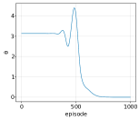
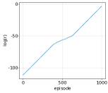
Figure 1: Left: midpoint of interval enclosure of a proven persistent solution (see Appendix Tab. 23). Right: log-scale of radius of the interval enclosure. Calculations done at 163 bit precision, the minimum possible for this solution at episode length 1000.

5.2 Computer-assisted Proofs of Periodic Orbits

For $x=(x_{1},\dots,x_{n})$, let $||x||=\max\{|x_{1}|,\dots,|x_{n}|\}$. The following is the core of our CAPs.

Theorem 5.1.

Let $G:U\rightarrow\mathbb{R}^{n}$ be continuously differentiable, for $U$ an open subset of $\mathbb{R}^{n}$. Let $\overline{x}\in\mathbb{R}^{n}$ and $r^{*}\geq 0$. Let $A$ be a $n\times n$ matrix of full rank. Suppose there exist real numbers $Y$, $Z_{0}$ and $Z_{2}$ such that

$$||AG(\overline{x})|| \leq Y,$$ (1)

$$||I-ADG(\overline{x})|| \leq Z_{0}$$ (2)

$$\sup_{|\delta|\leq r^{*}}||A(DG(\overline{x}+\delta)-DG(\overline{x}))|| \leq Z_{2},$$ (3)

where $DG(x)$ denotes the Jacobian of $G$ at $x$, and the norm on matrices is the induced matrix norm. If $Z_{0}+Z_{2}<1$ and $Y/(1-Z_{0}-Z_{2})\leq r_{*}$, the map $G$ has a unique zero $x$ satisfying $||x-\overline{x}||\leq r$ for any $r\in(Y/(1-Z_{0}-Z_{2}),r_{*}]$.

A proof can be completed by following Thm 2.1 in [9]. In Sec. 5.3, we identify $G$ whose zeroes correspond to POs. Conditions (1)–(3) imply that the Newton-like operator $T(x)=x-AG(x)$ is a contraction on the closed ball centered at the approximate zero $\overline{x}$ with radius $r>0$. Being a contraction, it has a unique fixed point ($x$ such that $x=T(x)$) by the Banach fixed point theorem. As $A$ is full rank, $G(x)=0$, hence an orbit exists. The radius $r$ measures how close the approximate orbit $\overline{x}$ is to the exact orbit, $x$. The contraction is rigorously verified by performing all necessary numerical computations using interval arithmetic. The technical details appear in App. D.2.

5.3 Set-up of the Nonlinear Map

A PO is a finite MDP trajectory. Let the step size be $h$, and let the period of the orbit be $m$. We present a nonlinear map that encodes (as zeroes of the map) POs when $h$ is fixed. However, for technical reasons (see App. E), it is possible for such a proof to fail. If Alg. 2 fails to prove the existence of an orbit with a fixed step size $h$, we fall back to a formulation where the step size is not fixed, which is more likely to yield a successful proof. This alternative encoding map $G_{2}$ is presented in App. D.1. Given $h$, pick $g(h,\cdot)\in\{g_{\rm E},g_{\rm SI}\}$ one of the discrete dynamical systems used for numerically integrating the ODE. Let $p$ be the dimension of the state space, so $g(h,\cdot):\mathbb{R}^{p}\rightarrow\mathbb{R}^{p}$. We interpret the first dimension of $\mathbb{R}^{p}$ to be the angular component, so that a periodic orbit requires a shift by a multiple of $2\pi$ in this variable. Given $h$, the number of steps $m$ (i.e. period of the orbit) and the number of signed rotations $j$ in the angular variable, POs are zeroes of the map (if and only if) $G_{1}:\mathbb{R}^{pm}\rightarrow\mathbb{R}^{pm}$, defined by

$$G_{1}(X)=\begin{pmatrix}x_{0}-g(h,x_{m})+(j2\pi,\mathbf{0})\\ x_{1}-g(h,x_{0})\\ x_{2}-g(h,x_{1})\\ \vdots\\ x_{m}-g(h,x_{m-1})\end{pmatrix},$$

where $\mathbf{0}$ is the zero vector in $\mathbb{R}^{p-1}$, $X=(x_{1},\dots,x_{m})$ for $x_{i}\in\mathbb{R}^{p}$, and $x_{1},\dots,x_{m}$ are the time-ordered states.

6 Persistent Orbits in Controlled Pendulum

When constructing controllers using machine learning or statistical methods, the most often used criterion for measuring their quality is the mean return from performing many test episodes. The mean return may be a deceptive metric for constructing robust controllers. More strongly, our findings suggest that mean return is not correlated to the presence of periodic orbits or robustness. One would typically expect a policy with high mean return to promote convergence toward states that maximize the return for any initial condition (IC) and also for other numerical schemes. Our experiments revealed reasons to believe this may be true for deep NN controllers. However, in the case of simple symbolic controllers, singular persistent solutions exist that accumulate large negative returns at a fast pace. By persistent solutions we mean periodic orbits that remain $\varepsilon$ away from the desired equilibrium. This notion we formalize in Sec. 7.1. We emphasize that all of the periodic orbits that we prove are necessary stable in the usual Lyapunov sense, i.e., the solutions that start out near an equilibrium stay near the equilibrium forever, and hence feasible in numerical simulations. We find such solutions for controllers as provided in the literature and constructed by ourselves employing Alg. 1. We emphasize that our findings are not only numerical, but we support them with (computer-assisted) mathematical proofs of existence.

6.1 Landajuela et. al [24] Controller

First, we consider the symbolic low complexity controller for the pendulum $a=-7.08s_{2}-(13.39s_{2}+3.12s_{3})/s_{1}+0.27$, derived in [24] (with model given in App. A.1), where $s_{1}=\cos{\theta}$, $s_{2}=\sin{\theta}$, $s_{3}=\omega=\theta^{\prime}$, and $a$ is the control input. While this controller looks more desirable than a deep NN with hundreds thousand of parameters, its performance changes dramatically when using slightly different transition function at test-time, i.e., halved $h$ ($F_{test}({\rm SI},0.025)$) or the explicit Euler scheme ($F_{test}({\rm E},0.05)$). Trajectories in Fig. 2 illustrate that some orbits oscillate instead of stabilizing at the equilibrium $\hat{s}=\hat{\theta}=0\text{ mod }2\pi$. The average return significantly deteriorates for the modified schemes and the same ICs compared to $F_{train}({\rm SI},0.05)$; see Tab. 1. Such issues are present in deep NN controllers and small distilled NN to a significantly lower extent. We associate the cause of the return deterioration with existence of ’bad’ solutions – persistent periodic orbits (POs) (formal Def. 7.1). Using CAPs (c.f., Sec. 5) we obtain:

Theorem 6.1.

For $h\in H=\{0.01,0.005,0.0025,0.001\}$, the nonlinear pendulum system with controller $a$ from [24] described in the opening paragraph of Section 6.1 has a periodic orbit (PO) under the following numerical schemes;

1) (SI) with step size $h\in H$,

2) (E) at $h=0.05$ (native), and for all $h\in H$.

The identified periodic orbits are persistent (see Def. 7.2) and generate minus infinity return for infinite episode length, with each episode decreasing the reward by at least 0.198.

(a) (SI), $h=0.05$ (native)

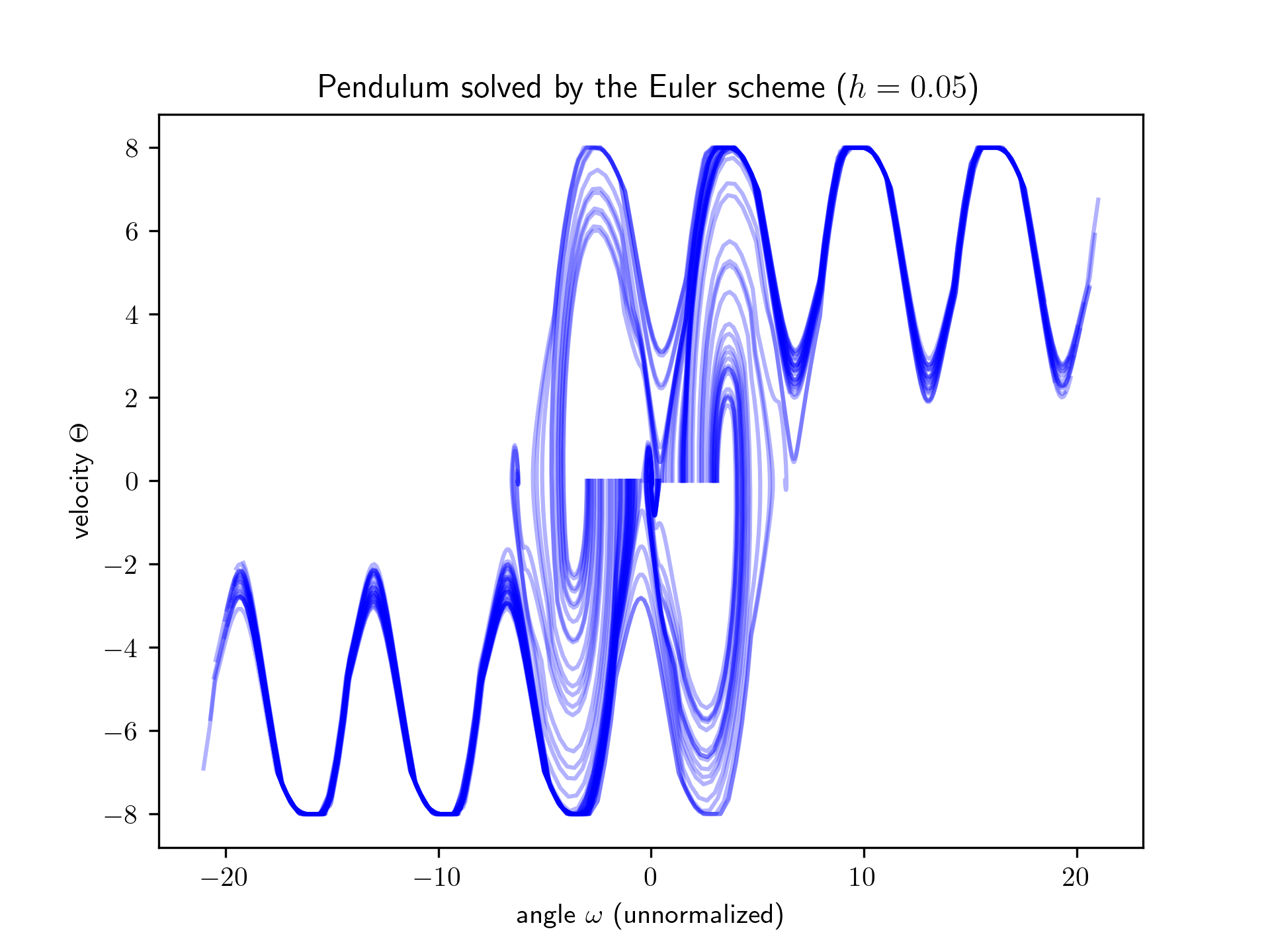
(b) (E), $h=0.05$

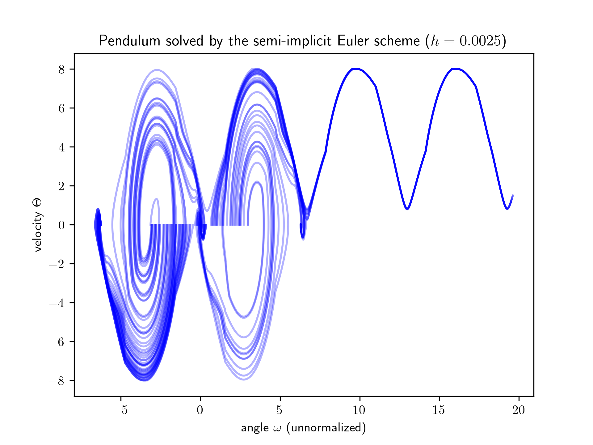
(c) (SI), $h=0.025$

Figure 2: $100$ numerical simulations with IC $\omega=0$ and $\theta$ sampled uniformly, time horizon set to $T=6$, $x$-axis shows the (unnormalized) $\omega$, and $y$-axis $\theta$. In (a), all IC are attracted by an equilibrium at $\omega=0\mbox{mod}2\pi$, $\theta=0$. Whereas when applying different $F_{test}$, (b) and (c) show existence of attracting periodic solutions (they can be continued infinitely as our theorems demonstrate).

6.2 Our Controllers

The issues with robustness and performance of controllers of Sec. 6.1 may be an artefact of a particular controller construction rather than a general property. Indeed, that controller had a division by $s_{1}$. To investigate this further we apply Alg. 1 for constructing symbolic controllers of various complexities (without divisions). Using Alg. 1 we distill a small NN (single hidden layer with $10$ neurons) for comparison. In step 2 we use fine-tuning based on either analytic gradient or CMA-ES, each leading to different controllers. The studied controllers were trained using the default transition $F_{train}({\rm SI},0.05)$, and for testing using $F_{test}({\rm E},0.05)$, $F_{test}({\rm E},0.025)$, $F_{test}({\rm SI},0.05)$, $F_{test}({\rm SI},0.025)$.

Tab. 1 reveals that the average returns deteriorate when using other numerical schemes for the symbolic controllers obtained using Alg. 1, analogous to the controller from [24]. The average return discrepancies are very large as well. We emphasize that all of the studied metrics for the symbolic controllers are far from the metrics achieved for the deep NN controller. Terminating Alg. 1 at step 2 results in a very bad controller achieving mean return only of $-1061$, i.e., as observed in the previous works the symbolic regression over a dataset sampled from a trained NN is not enough to construct a good controller. Analogous to Theorem 6.1, we are able to prove the following theorems on persistent periodic orbits (Def. 7.1) for the controllers displayed in Table 1.

Theorem 6.2.

For $h\in H=\{0.025,0.0125\}$, the nonlinear pendulum system with controller generated by analytic gradient refinement in Tab. 1 has POs under

1) (SI) with $h\in H$ and at the native step size $h=0.05$,

2) (E) with $h\in H$.

The identified periodic orbits are persistent (see Def. 7.2) and generate minus infinity return for infinite episode length, with each episode decreasing the reward by at least $0.18$.

Theorem 6.3.

For $h=0.0125$ and $h=0.05$ (native) with scheme (E), the nonlinear pendulum system with controller generated by CMA-ES refinement in Tab. 1 has POs which generate minus infinity return for infinite episode length, with each episode decreasing the reward by at least 0.20.

Table 1: Comparison of different controllers for the pendulum. Mean $\pm$ std.dev. rounded to decimal digit, returns over $100$ episodes reported for different $F_{test}$ (larger the better). $F_{test}=F_{train}$ marked in bold. In this case mean return is equal to negative accumulated penalty. Absolute return discrepancies measure discrepancy in episodic return between different schemes (E/SI) for the same IC (smaller the better). The meaning of observation vector at given time $t$, $x_{0}=\cos{\theta(t)}$, $x_{1}=\sin{\theta(t)}$, $x_{2}=\omega(t)=\theta(t)^{\prime}$.

		mean return for given $F_{test}$
		$\mathbf{h=0.05}$		$h=0.025$		discrepancy
origin	formula	SI	E	SI	E	return E / SI
Alg. 1, 3.analytic (symb. $k=9$)	$((((1.30\cdot x_{2}+4.18\cdot x_{1})x_{0})+0.36x_{1})/-0.52)$	$-207\pm 183$	$-604\pm 490$	$-431\pm 396$	$-910\pm 853$	$479\pm 416$
Alg. 1, 3.CMA-ES (symb. $k=9$)	$((((-10.59x_{2}+-42.47x_{1})x_{0})+1.2x_{1})/5.06)$	$-165\pm 113$	$-659\pm 461$	$-331\pm 225$	$-1020\pm 801$	$538\pm 401$
Alg. 1, small NN	$10$ neurons distilled small NN	$-157\pm 99$	$-304\pm 308$	$-311\pm 196$	$-290\pm 169$	$188\pm 285$
[24] $(a_{1})$	$-7.08x_{1}-(13.39x_{1}+3.12x_{2})/x_{0}+0.27$	$-150\pm 87$	$-703\pm 445$	$-318\pm 190$	$-994\pm 777$	$577\pm 401$
TD3 training	deep NN	$-149\pm 86$	$-138\pm 77$	$-298\pm 171$	$-278\pm 156$	$18\pm 38$

7 Systematic Robustness Study

We consider a controller to be robust when it has “good" return statistics at the native simulator and step size, which persist when we change simulator and/or decrease step size. If a degradation of return statistics on varying the integrator or step size is identified, we wish to identify the source.

7.1 Background on Persistent Solutions and Orbits

Consider a MDP tuple $(\mathcal{S},\mathcal{A},F,r,\rho_{0},\gamma)$, a precision parameter $\varepsilon>0$, a policy $\pi\colon\mathcal{S}\to\mathcal{A}$ (trained using $F_{train}$ and tested using $F_{test}$), a desired equilibrium $\hat{s}$ (corresponding to the maximized reward $r$), and episode length $N$.

Definition 7.1.

We call a persistent periodic orbit (PO) (of period $n$) an infinite MDP trajectory $(s_{0},a_{0},r_{1},s_{1},a_{1},\dots)$, such that $s_{kn}=s_{0}$ for some $n>1$ and all $k\in\mathbb{N}$, and such that $\|\hat{s}-s_{j}\|>\varepsilon$ for all $j\geq 0$.

Definition 7.2.

A finite MDP trajectory of episode length $N$ $(s_{0},a_{0},p_{1},s_{1},a_{1},\dots,s_{N})$ such that $\|\hat{s}-s_{j}\|>\varepsilon$ for all $0\leq j\leq N$ is called a persistent solution.

Locating the objects in dynamics responsible for degradation of the reward is not an easy task, as they may be singular or local minima of a non-convex landscape. For locating such objects we experimented with different strategies, but found the most suitable the evolutionary search of penalty maximizing solutions. The solutions identified using such a procedure are necessarily stable. We introduce a measure of ’badness’ of persistent solutions and use it as a search criteria.

Definition 7.3.

We call a penalty value, a function $p\colon\mathcal{S}\times\mathcal{A}\to\mathbb{R}_{+}$, such that for a persistent solution/orbit the accumulated penalty value is bounded from below by a set threshold $M\gg 0$, that is $\sum_{i=0}^{N-1}{p(s_{i},a_{i})}\geq M$.

Remark 7.4.

The choice of particular penalty in Def. 7.3 depend on the particular studied example. We choose the following penalties in the studied problems.

1. $p(s,a)=-r(s,a)$ for pendulum.

2. $p(s,a)=-r(s)+0.5(\theta^{\prime})^{2}+0.5(x^{\prime})^{2}$ for cartpole swing-up. Subtracting from the native reward value $r(s)=\cos{\theta}$ the scaled sum of squared velocities (the cart and pole) and turning off the episode termination condition. This allows capturing orbits that manage to stabilize the pole, but are unstable and keep the cart moving. The threshold $M$ in Def. 7.3 can be set by propagating a number of trajectories with random IC and taking the maximal penalty as $M$.

Remark 7.5.

For a PO, the accumulated penalty admits a linear lower bound, i.e. $\sum_{m=0}^{n-1}p(s_{m},a_{m})\geq Cn$ for some $C>0$. Thm. 6.1 implies $C=0.14$ for the POs in Tab. 6 in the Appendix.

7.2 Searching for and Proving Persistent Orbits

We designed a pipeline for automated persistent/periodic orbits search together with interval proof certificates. By an interval proof certificate of a PO we mean interval bounds within which a CAP that the orbit exist was carried out applying the Newton scheme (see Sec. 5.2), whereas by a proof certificate of a persistent solution (which may be a PO or not) we mean interval bounds for the solution at each step, with a bound for the reward value, showing that it does not stabilize by verifying a lower bound $\|\hat{s}-s_{t}\|>\varepsilon$. The search procedure is implemented in Python, while the CAP part is in Julia, refer Sec. 5 for further details.

Algorithm 2 Persistent Solutions/Orbits Search & Prove

0:  $F_{test}$; control policy $\pi$; $h$-parameters of the evolutionary search; penalty function $p$; trajectory length; search domain;

0:  interval certificates of persistent/periodic orbits;

1:  for each MDP do

2:    for  number of searches do

3:       initialize CMA-ES search within specified bounds;

4:       search for a candidate maximizing penalty $p$ during the fixed episode length;

5:    end for

6:    order found candidates w.r.t. their $p$ value;

7:  end for

8:  for each candidate do

9:    search for nearby periodic orbit with Newton’s method correction applied to suitable sub-trajectory;

10:    if potential periodic orbit found then

11:       attempt to prove existence of the orbit with Thm. 5.1;

12:       if proof successful then

13:          return an interval certificate of the orbit;

14:       else

15:          return proof failure;

16:       end if

17:    else

18:       return periodic orbit not found;

19:    end if

20:    produce and return an interval certificate of the uncontrolled solution;

21:  end for

7.3 Findings: Pendulum

Changing simulator or step size resulted in substantial mean return loss (see Tab. 1), and simulation revealed stable POs (see Fig. 2). We proved existence of POs using the methods of Section 5.2–5.3. Proven POs are presented in tables in App. F. See also Fig. 3, where an persistent solution shadows an unstable PO before converging to the stable equilibrium. We present proven persistent solutions in the tables in App. F.

Comparing the mean returns in Tab. 1 we immediately see that deep NN controller performance does not deteriorate as much as for the symbolic controller, whereas the small net is located between the two extremes. This observation is confirmed after we run Alg. 2 for the symbolic controllers and NN. In particular, we did not identify any stable periodic orbits or especially long persistent solutions. However, the Deep NN controller is not entirely robust, admitting singular persistent solutions achieving returns far from the mean; refer to Tab. 4. On the other hand, the small $10$ neuron NN also seems to be considerably more robust than the symbolic controllers. For the case $F_{test}({\rm E},0.05)$ the average returns are two times larger than for the symbolic controllers, but still two times smaller than for the deep NN. However, in the case $F_{test}({\rm E},0.05)$, the average returns are close to those of the deep NN contrary to the symbolic controllers. The small NN compares favorably to symbolic controllers in terms of E/SI return discrepancy metrics, still not reaching the level of deep NN. This supports our earlier conjecture (Sec. 1) that controller robustness is proportional to the parametric complexity.

Table 2: Examples of persistent solutions found by the persistent solutions Search & Prove Alg. 2 for the pendulum maximizing accumulated penalty, episodes of fixed length $N=1000$. The found persistent solutions were the basis for the persistent orbit/solution proofs presented in App. F.

controller	MDP	$\sum{r(s,a)}$
Alg. 1 ( $k=9$)	(SI) $h=0.05$	$-9869.6$
Alg. 1 ( $k=9$)	(SI) $h=0.025$	$-1995.7$
Alg. 1 small NN	(SI) $h=0.05$	$-926.8$
Alg. 1 small NN	(SI) $h=0.025$	$-1578.4$
Alg. 1 small NN	(E) $h=0.05$	$-747.3$
[24] $(a_{1})$	(SI) $h=0.05$	$-873.8$
[24] $(a_{1})$	(SI) $h=0.025$	$-1667.6$
[24] $(a_{1})$	(E) $h=0.05$	$-5391.1$
deep NN	(SI) $h=0.05$	$-426.4$
deep NN	(SI) $h=0.025$	$-818.6$
deep NN	(E) $h=0.05$	$-401.4$

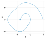
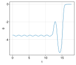
Figure 3: A persistent solution with poor reward $\approx-7527$ over episode length 1000 with step size $h=0.0125$, plotted until near-stabilization at $t=17.825$. Left: plot in phase space. Right: time series of $\theta$. Other data for this solution is in Appendix Tab.22.

7.4 Findings: Cartpole Swing-Up

Table 3: Mean $\pm$ std.dev. reported, rounded to single decimal digits, of returns over $100$ episodes reported for different $F_{test}$ (larger the better). $F_{test}=F_{train}$ marked in bold. Return discrepancies measure discrepancy in episodic return between different schemes (E/SI) for the same IC (smaller the better). The formula for the symbolic controller with $k=21$ is appears in Appendix Tab. 27

	mean return for given $F_{test}$
	$\mathbf{h=0.01}$		$h=0.005$		discrepancy
origin	SI	E	SI	E	return E / SI
Alg. 1, 3.CMA-ES (symb. $k=21$)	$220.2\pm 96.7$	$334.3\pm 37$	$474.6\pm 194.3$	$632.2\pm 119.3$	$121.9\pm 88.9$
Alg. 1, small NN ($25$ neurons)	$273.3\pm 128.7$	$332.9\pm 79.2$	$585.1\pm 229.1$	$683.7\pm 103.3$	$86.6\pm 135.1$
TD3 training	$381.2\pm 9.1$	$382.9\pm 9$	$760.9\pm 18.4$	$764.0\pm 18.1$	$1.7\pm 0.9$

We computed the mean return metrics for a representative symbolic controller, a distilled small NN controller and the deep NN, see Tab. 3. For the symbolic controller, the average return deteriorates more when changing the simulator’s numerical scheme to other than the native ($F_{train}({\rm E},0.01)$). Notably, the E/SI discrepancy is an order of magnitude larger than in the case of deep NN. As for the pendulum, the small NN sits between the symbolic and deep NN in terms of the studied metrics. We computed the mean accumulated shaped penalty $p(s,a)=-r(s)+0.5(\theta^{\prime})^{2}+0.5(x^{\prime})^{2}$ for the selected controllers in Tab. 5. The contrast between the deep NN and the symbolic controller is clear, with the small NN being in between those two extremes. The mean penalty is a measure of the prevalence of persistent solutions. However, we emphasize that the Deep NN controller is not entirely robust and also admits singular persistent solutions with bad returns, refer to Tab. 4. Rigorously proving the returns for the deep NN was not possible in this case; see Rem. 7.8.

Investigating the persistent solutions found with Alg. 2 in Fig. 4 we see that in case $F_{test}({\rm SI},0.01)$ the symbolic controller admits bad persistent solutions with $x_{t}$ decreasing super-linearly, whereas $\theta$ stabilizes at $\theta\sim 0.01$. In contrast, the deep NN exhibits fairly stable control with small magnitude oscillations. This example emphasizes the shaped penalty’s usefulness in detecting such bad persistent solutions. We can see several orders of magnitude differences in the accumulated penalty value for the deep NN controller vs. the symbolic controller case. We identify and rigorously prove an abundance of persistent solutions for each of the studied symbolic controllers. For example, we can prove:

Theorem 7.6.

For the symbolic controller with complexity $k=21$ and native step size $h=0.01$, there are 2000-epsiode persistent solutions of the cartpole swing-up model with accumulated penalty $\geq 2.66\times 10^{5}$ for the explicit scheme, and $\geq 3.77\times 10^{5}$ for the semi-implicit scheme. With the Small NN controller, the conclusions hold with accumulated penalties $\geq 6263$ and $\geq 2.68\times 10^{6}$.

Table 4: Examples of persistent solutions found by the transient solutions Search & Prove Alg. 2 for the cartpole-swingup maximizing the accumulated penalty, episodes of fixed length $N=2000$ without taking into account the termination condition. The found persistent solutions were the basis for the persistent orbit/solution proofs presented in App. G

controller	MDP	$\sum{r(s,a)}$
Alg. 1 ( $k=21$)	(SI) $h=0.01$	$-41447.2$
Alg. 1 ( $k=21$)	(SI) $h=0.005$	$-11204.3$
Alg. 1 ( $k=21$)	(E) $h=0.01$	$-29878.0$
Alg. 1 ( $k=21$)	(E) $h=0.005$	$-8694.3$
Alg. 1 small NN	(SI) $h=0.01$	$-2684696.8$
Alg. 1 small NN	(SI) $h=0.005$	$-798442.3$
Alg. 1 small NN	(E) $h=0.01$	$-520.9$
Alg. 1 small NN	(E) $h=0.005$	$-2343.8$
deep NN	(SI) $h=0.01$	$306.6$
deep NN	(SI) $h=0.005$	$-396074.9$
deep NN	(E) $h=0.01$	$226.5$
deep NN	(E) $h=0.005$	$-1181.7$

We demonstrate persistent solutions for each considered controller in Tab. 4. The found persistent solutions were the basis for the persistent orbit/solution proofs presented in App. G. The symbolic and small NN controllers admit much worse solutions with increasing velocity, as illustrated in Fig. 4(b). Deep NN controllers admit such bad solutions when tested using smaller time steps ($(E,0.005),(SI,0.005)$); see examples in Tab. 4. They also exhibit persistent periodic solutions, albeit with a small $\epsilon$; see Fig. 4(a). We have proven the following.

Theorem 7.7.

For $h$ close to $0.005$ and $h=0.01$ (native), the cartpole swing-up model has POs for (E) and (SI) with the deep NN controller. The mean penalties along orbits are greater than $-0.914$ and are persistent with $\epsilon\geq 0.036$.

Remark 7.8.

We were not able to rigorously compute the penalty values of the persistent solutions for the deep NN controller due to wrapping effect of interval arithmetic calculations [38], which is made much worse by the width of the network (400,300) and the long epsiode length (which introduces further composition). However, this is not a problem for the periodic orbits: we enclose them using Theorem 5.1, which reduces the wrapping effect.

Table 5: Comparison of different controllers for the cartpole swing-up for $h=0.01$. Mean and std.dev. (after $\pm$) reported of accumulated penalties $\sum p(s_{k})=\sum-r(s_{k})+0.5(\theta_{k}^{\prime})^{2}+0.5(x_{k}^{\prime})^{2}$ (larger the worse) over $100$ episodes reported for different $F_{test}$. $F_{test}=F_{train}$ marked in bold. Controllers same as in Tab. 3.

origin	SI	E
Alg. 1, 3.CMA-ES (symb. $k=21$)	$3123.0\pm 719.9$	$2257.2\pm 234.1$
Alg. 1, small NN ($25$ neurons)	$1413.4\pm 9670.1$	$404.2\pm 148.4$
TD3 training	$335.7\pm 64.7$	$425.6\pm 72.1$

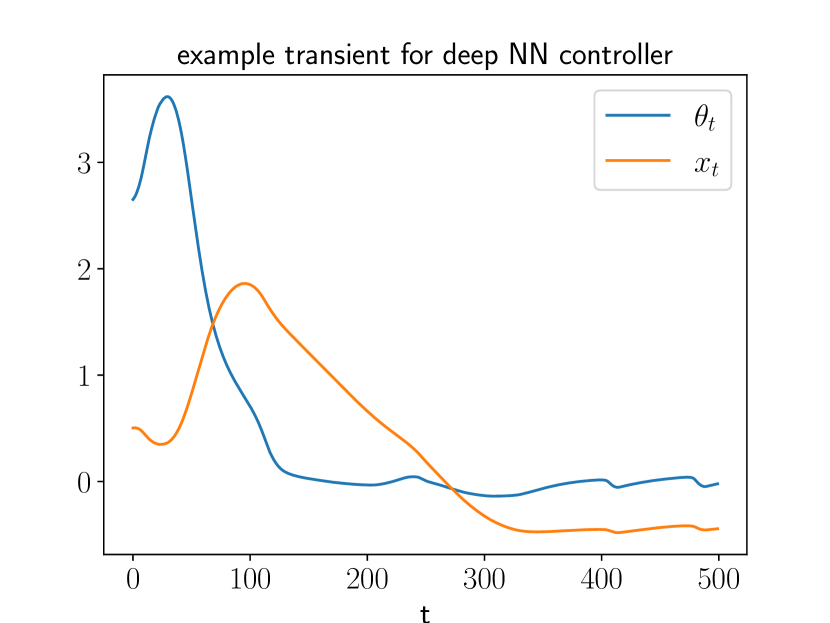
(a) Deep NN controller

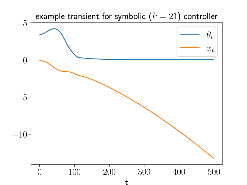
(b) a symbolic controller

Figure 4: The persistent solutions (evolution of $(\theta,x)$ (Def. 7.2) for cartpole swing-up problem found with Alg. 2 that maximize accumulated penalty $\sum p(s,a)=\sum{-r(s)+0.5(\theta^{\prime})^{2}+0.5(x^{\prime})^{2}}$ over episodes of length $2000$ without terminations, using SI with $h=0.01$. (a) $\sum{p(s,a)}=-306$; (b) $\sum{p(s,a)}=37746$.

8 Codebase

Our full codebase is written in Python and Julia shared in a github repository [2]. The reason why the second part of our codebase is written in Julia is the lack of a suitable interval arithmetic library in Python. The Python part of the codebase consists of four independent parts – scripts: deep NN policy training, symbolic/small NN controller regression, regressed controller fine-tuning and periodic orbit/persistent solution searcher. All controllers that we use are implemented in Pytorch [28]. For the deep NN policy training we just use the Stable-baselines 3 library [30], which outputs a trained policy (which achieved the best return during training) and the training replay buffer of data. For the symbolic regression we employ the PySR lib. [7]. For the regressed controller fine-tuning we employ the pycma CMA-ES implementation [18]. Our implementation in Julia uses two external packages: IntervalArithmetic.jl [33] (for interval arithmetic) and ForwardDiff.jl [31] (for forward-mode automatic differentiation). These packages are used together to perform the necessary calculations for the CAPs.

9 Conclusion and Future Work

Our work is a first step towards a comprehensive robustness study of deep NN controllers and their symbolic abstractions, which are desirable for deployment and trustfulness reasons. Studying the controllers’ performance in a simple benchmark, we identify and prove existence of an abundance of persistent solutions and periodic orbits. Persistent solutions are undesirable and can be exploited by an adversary. Future work will apply the developed methods to study higher dimensional problems often used as benchmarks for continuous control.

10 Acknowledgements

The project is financed by the Polish National Agency for Academic Exchange. The first author has been supported by the Polish National Agency for Academic Exchange Polish Returns grant no. PPN/PPO/2018/1/00029 and the University of Warsaw IDUB New Ideas grant. This research was supported in part by PL-Grid Infrastructure.

Appendix A Studied Dynamical Systems

In this section we describe the details of studied problems. The continuous dynamical system with their discretizations.

A.1 Pendulum

A.1.1 Continuous System

We study numerical discretizations of the following continuous dynamical system governing the motion of a simple pendulum

$$\theta^{\prime\prime}(t)=\frac{3u(t)}{l^{2}m}+\frac{3g\sin(\theta(t))}{2l},$$

where $\theta(t)$ is the current angle at time $t$ of the pendulum, and $u(t)$ is the controller input, $l$, $m$, $g$ are the pendulum length, mass and the gravitational constant respectively. We set them to the values used in the environment code, i.e., $l=1,m=1,g=10$. The uncontrolled model admits the unstable equilibrium at $\theta=0$, and the stable equilibrium at $\theta=\pm\pi$.

Let us introduce auxiliary variable $\omega=\theta^{\prime}$, and the following extended system

$$\theta^{\prime}(t) =\omega(t),$$ (4a)

$$\omega^{\prime}(t) =\frac{3u(t)}{l^{2}m}+\frac{3g\sin(\theta(t))}{2l},$$ (4b)

let us denote $x(t)=[\theta(t),\omega(t)]$, and by $f(x(t))$ we denote the right hand side of (4).

A.1.2 Discrete Systems

In practice, we will study various discrete dynamical systems arising from discretizing (4) with timesteps $t_{0},t_{1},\dots,t_{k}$ and fixed constants $l$, $m$, $g$, and employing various numerical methods mentioned below.

The particular numerical methods that we study include

Explicit Euler, fixed time-step

$$t_{k} =t_{k-1}+h,$$

$$\bar{\theta}_{k} =\bar{\theta}_{k-1}+h\bar{\omega}_{k-1}(t),$$

$$\bar{\omega}_{k} =\lfloor\bar{\omega}_{k-1}+hf^{2}(x_{k-1},\lfloor u_{k-1}\rfloor)\rfloor,$$

we denote the formula for $x_{k}=(\bar{\theta}_{k},\bar{\omega}_{k})$ by $g_{ee}(t_{k-1},x_{k-1})$. Where $h$ is the uniform fixed time-step. We denote $\lfloor u_{k-1}\rfloor$, and $\lfloor\bar{\omega}_{k}\rfloor$ denote the clipped values, i.e. if $u_{k-1}$ exceeds the range $[-2,2]$ its value is clipped to the closest value in the range (whereas the velocity is clipped to the range $[-8,8]$).

Semi-implicit Euler

This is the original numerical method used for solving the pendulum dynamics in the OpenAI gym package [5] (with $h=0.05$)

$$t_{k} =t_{k-1}+h,$$

$$\bar{\omega}_{k} =\lfloor\bar{\omega}_{k-1}+hf^{2}(x_{k-1},\lfloor u_{k-1}\rfloor)\rfloor,$$

$$\bar{\theta}_{k} =\bar{\theta}_{k-1}+h\bar{\omega}_{k},$$

where $x_{k}=(\bar{\theta}_{k},\bar{\omega}_{k})$, and we denote the formula for $x_{k}$ by $g_{sie}(t_{k-1},x_{k-1})$. We call the method semi-explicit, however it is cooked up for the particular case of the pendulum. In the first step the new velocity is computed and then in the second step the angle is updated using the new velocity.

Appendix B Cartpole Swing-up

B.1 Continuous System

We used the implementation [1], which is slightly modified version used in [15]. The motion of the cartpole is determined by the following dynamical system

$$\theta^{\prime\prime} =\left(-3(m_{p}+l)(\theta^{\prime})^{2}\sin{\theta}\cos{\theta}+6(m_{p}+m_{c})g\sin{\theta}+6(u-fx^{\prime})\cos{\theta}\right)/(4(m_{p}+m_{c})l-3(m_{p}+l)\cos^{2}{\theta})=f_{1}(\theta,\theta^{\prime},x^{\prime}),$$

$$x^{\prime\prime} =\left(-2(m_{p}+l)\cdot(\theta^{\prime})^{2}\cdot\sin{\theta}+3m_{p}g\sin{\theta}\cos{\theta}+4u-4fx^{\prime}\right)/(4(m_{p}+m_{c})-3m_{p}\cos^{2}{\theta})=f_{2}(\theta,\theta^{\prime},x^{\prime},u),$$

where $u$ is the control input at given time (input from range $[-1,1]$ is multiplied by $10$). We set the constants as in the original environment code, pole mass $m_{p}=0.5$, pole length $l=0.6$, cart mass $m_{c}=0.5$, gravity const. $g=9.82$, fricition const. $f=0.1$

B.2 Discrete Systems

The continuous dynamical system above is discretized using two numerical schemes that we present below.

B.2.1 Explicit Euler

This is the numerical method applied in the original implementation (with $h=0.01$).

$$t_{k} =t_{k-1}+h,$$

$$x_{k} =x_{k-1}+hx^{\prime}_{k-1},$$

$$\theta_{k} =\theta_{k-1}+h\theta^{\prime}_{k-1},$$

$$x^{\prime}_{k} =x^{\prime}_{k-1}+h\cdot f_{2}\left(\theta_{k-1},\theta^{\prime}_{k-1},x^{\prime}_{k-1},10\cdot\lfloor u_{k-1}\rfloor\right),$$

$$\theta^{\prime}_{k} =\theta_{k-1}^{\prime}+h\cdot f_{1}\left(\theta_{k-1},\theta^{\prime}_{k-1},x^{\prime}_{k-1}\right),$$

where $\lfloor\cdot\rfloor$ is clipping the input to interval $[-1,1]$.

B.2.2 Semi-implicit Euler

This is another numerical method that we implemented for our robustness study, based on the method used in pendulum (with $h=0.01$).

$$t_{k} =t_{k-1}+h,$$

$$x^{\prime}_{k} =x^{\prime}_{k-1}+h\cdot f_{2}\left(\theta_{k-1},\theta^{\prime}_{k-1},x^{\prime}_{k-1},10\cdot\lfloor u_{k-1}\rfloor\right),$$

$$\theta^{\prime}_{k} =\theta_{k-1}^{\prime}+h\cdot f_{1}\left(\theta_{k-1},\theta^{\prime}_{k-1},x^{\prime}_{k-1}\right),$$

$$x_{k} =x_{k-1}+hx^{\prime}_{k},$$

$$\theta_{k} =\theta_{k-1}+h\theta^{\prime}_{k}.$$

By the semi-implicit scheme in this case we mean that velocities $x_{k}^{\prime},\theta_{k}^{\prime}$ are first updated using the accelerations from the previous step (depending on $\theta_{k-1},\theta^{\prime}_{k-1},x^{\prime}_{k-1}$), then positions $x_{k},\theta_{k}$ are updated using the current velocities $x^{\prime}_{k},\theta^{\prime}_{k}$.

Appendix C TD3 RL agents training curves

We report on the RL training of the deep NN controllers studied in this work utilizing the TD3 [12] algorithm. The resulting plots showing training episodic returns are presented in Fig. 5.

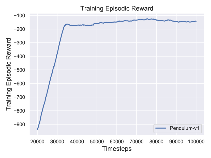
(a) Pendulum

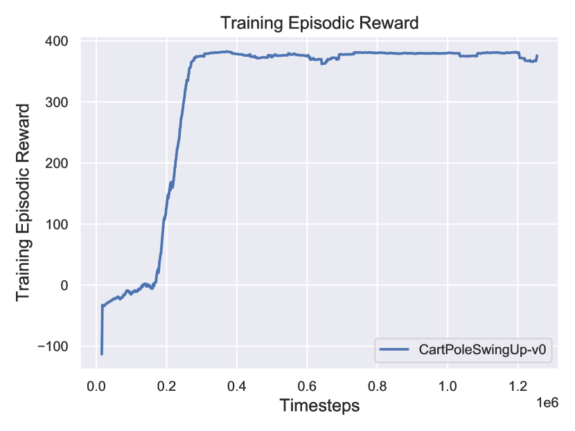
(b) Cartpole Swing-up

Figure 5: Obtained TD3 training curves using the SB3 implementation [30]. As the ’deep NN’ controller we pick the best according to the episodic return checkpoint obtained within the number of episodes shown.

Appendix D Rigorous proof methodology: further details

Here we provide additional details concerning the maps $G$ required for computer-assisted proofs, and the implementation.

D.1 The map $G$ for the variable step size case

Suppose we want to treat $h$ as variable, rather than an a priori fixed constant. Let $\eta:\mathbb{R}^{p}\rightarrow\mathbb{R}$ be given, and define $G_{2}:\mathbb{R}^{pm+1}\rightarrow\mathbb{R}^{pm+1}$ by

$${G_{2}(X)=\begin{pmatrix}\eta(x_{0})\\ x_{0}-g(h,x_{m})+(j2\pi,\mathbf{0})\\ x_{1}-g(h,x_{0})\\ x_{2}-g(h,x_{1})\\ \vdots\\ x_{m}-g(h,x_{m-1})\end{pmatrix},}$$

where $X=(h,x_{0},\dots,x_{m})$. $\eta$ compensates for the addition of another variable. In practice, we choose $\eta$ to be a linear function.

D.2 Implementation details

In our robustness study, the maps $G$ (e.g. $G_{1}$, $G_{2}$) used for computer-assisted proofs are not globally continuously differentiable. Indeed, we have 1) lack of smoothness of the symbolic controller representation (e.g. divisions by zero at some inputs, non-smooth ReLU activation function), and 2) discrete logic rules (e.g. clipping, piecewise-linear saturation) in the simulator and/or controller. This makes it difficult to verify that $G:U\rightarrow\mathbb{R}^{n}$ is locally (i.e. in $U$) continuously differentiable. We overcome this with a clever implementation-level trick: we implement $g$ (the discrete-time system defining $G_{1}$ and $G_{2}$) in such a way that Julia will return an error if $g$ is evaluated on an interval (or interval vector) input that contains a point where the function is either undefined or non-smooth. This ensures that successfully evaluating $G_{1}$ or $G_{2}$ in Julia on an interval automatically proves it is smooth there.

Let us go over how Theorem 5.1 is verified. First, we identify a candidate for a periodic orbit as in Section 7, denoted $\overline{x}$ and stored as a vector such that $G(\overline{x})\approx 0$. We use automatic differentiation to calculate $DG(\overline{x})$, and then calculate a machine inverse $A$. To get $Y$, we simply calculate $||AG(\overline{x})||$ using interval arithmetic, and let $Y$ be the interval supremum. We do the same thing for the bound $Z_{0}$. These choices result in (1) and (2) being satisfied. Note that if $Z_{0}+Z_{2}<1$, then $||I-ADG(\overline{x})||<1$ and it follows that $A$ must be full rank. To calculate $Z_{2}$, we use automatic differentiation to first calculate the Jacobian of $G$ at the interval representation of the closed ball (interval vector) $[\overline{x}]_{r^{*}}=\{x\in\mathbb{R}^{n}:||x-\overline{x}||\leq r^{*}\}.$ Note that $r^{*}$ must be specified beforehand. We compute $Z_{2}=\sup||A(DG([\overline{x}]_{r^{*}})-DG(\overline{x}))||,$ where $\sup$ denotes the interval supremum. This choice of $Z_{2}$ results in (3) being satisfied. We then compute $Y/(1-Z_{0}-Z_{2})$ and let $r$ be the result of rounding up to the next float. Finally, we check that $Y+r(Z_{0}+Z_{2}-1)<0$ and $r\leq r^{*}$, as desired.

To contrast, proofs of persistent solutions do not require Theorem 5.1. Instead, we reliably simulate persistent solutions by running the simulator initialized at a thin interval IC. In other words, we use interval arithmetic to rigorously track rounding errors caused by the numerical simulator. The amount of steps we can reliably simulate in this way is dependent on the precision of the number system.

Appendix E Persistence of periodic orbits under discretization

For a simple example that can be studied analytically, consider the harmonic oscillator $\ddot{x}=-x$. Transforming to polar coordinates via $x=r\cos\theta$ and $\dot{x}=r\sin\theta$, we get the two-dimensional ODE system

$$\dot{r}=0,\hskip 5.69054pt\dot{\theta}=1.$$

A periodic orbit corresponds to rotation, that is, $\theta\mapsto\theta+2\pi$. However, with the forward Euler integrator at step size $h$, step $k$ has coordinates $(r_{k},\theta_{k})=(r_{0},\theta_{0}+kh)$. Unless $h$ and $\pi$ are commensurate, a periodic orbit can not exist. In this case, the set $\{\theta_{k}\mod 2\pi,\hskip 2.84526ptk=1,2,\dots\}$ densely fills the interval $[0,2\pi]$. In the topological dynamics sense, this indicates that periodic orbits could persist under discretization as orbits equivalent to an irrational rotation of the circle $\mathbb{R}/\mathbb{Z}$. If $h$ and $\pi$ are commensurate – say, $am=b2\pi$ for some integers $m$ and $b$ – then $\theta_{m}=\theta_{0}+b2\pi$. Therefore, there is a $m$-step orbit. However, it could be that $m$ is extremely large.

To summarize, a periodic orbit in an ODE could persist as an $m$-step orbit for a possibly large $m$, or it could be equivalent to an irrational circle rotation. The example we saw is artificial, since its periodic orbits (for the ODE) come in continuous families parameterized by the radius in polar coordinates. However, the idea demonstrates why it might not be possible to (easily) prove a periodic orbit for a given step size $h$ and number of steps $m$, despite the appearance of a good numerical candidate.

Appendix F Proven periodic orbits and persistent solutions for the inverted pendulum

In the following pages, we catalogue the periodic orbits and persistent solutions we have proven for the inverted pendulum model. To improve readability, all initial angles, angular velocities and step sizes are truncated to five decimal places. In all cases, numbered controllers reference those in Table 7. For the periodic orbits (Table 8 through Table 17), we indicate if the step size is proven exactly (i.e. the map $G_{1}$ is used) or not. The direction column indicates if the orbit rotates counter-clockwise (direction = $+$) or clockwise (direction = $-$). For persistent solutions (Table 18 through Table 26), we integrate forward from ICs $(\theta_{0},\omega_{0})$ with the specified integrator. In the persistent solution tables, the time $T_{p}$ denotes one of the following:

• the first time where the solution satisfies $(\tilde{\theta},\omega)\in[0,10^{-2}]\times[-10^{-2},10^{-2}]$ for $\tilde{\theta}=\arccos(\cos(\theta))$, or

• if this does not occur within 1000 steps (episodes), then we let $T_{p}=1000h$.

Note that the step size $h$ of the integrator and the final time $T_{p}$ are related by the relationship $T_{p}=mh$, where $m$ is the number of simulation steps. The rewards and returns stated are midpoints of interval-value rewards, of which the latter are guaranteed to enclose the true value. The radii of these intervals are in all cases small, typically around $10^{-14}$.

Numerical Method	$h$	$m$	$\theta_{0}$	$\omega_{0}$	Max Reward
Explicit	0.05	28	3.94871	8.0	-0.64228
Explicit	0.025	55	4.10685	7.83862	-0.68942
Explicit	0.01	166	0.69262	1.59285	-0.33452
Explicit	0.005	358	0.69672	1.42118	-0.26396
Explicit	0.0025	721	0.69597	1.40667	-0.25791
Explicit	0.001	1839	0.29451	1.00288	-0.24372
Semi-Implicit	0.01	202	0.20564	1.02174	-0.19888
Semi-Implicit	0.005	398	0.69922	1.23635	-0.20352
Semi-Implicit	0.0025	760	0.6974	1.30669	-0.22475
Semi-Implicit	0.001	1870	0.48466	0.89362	-0.23343

Table 6: Summary data for the periodic orbits proven for the inverted pendulum model with the Landajuela et. al controller $a_{1}=-7.08s_{2}-(13.39s_{2}+3.12s_{3})/s_{1}+0.27$. All orbits complete a single counter-clockwise rotation.

Controller	Formula
7A AG	$-((1.074\cdot(x_{2}\cdot x_{0})+3.064\cdot x_{1})/0.482)$
9A AG	$-((((1.303\cdot x_{2}+4.180\cdot x_{1})\cdot x_{0})+0.364\cdot x_{1})/0.519)$
13A AG	$(((x_{2}\cdot 1.168+x_{1}\cdot 4.4618)\cdot x_{0})/((x_{2}\cdot(-x_{2}\cdot 0.014))-0.207))$
17A AG	$(((0.567\cdot x_{2}+2.032\cdot x_{1})\cdot x_{0}\cdot 1.381)/((x_{2}\cdot((x_{2}\cdot(x_{0}\cdot x_{0}))\cdot-0.034)-0.112))$
19A AG	$(((1.627\cdot x_{2}+(x_{1}/0.161))\cdot x_{0})/((((x_{1}/0.168)+0.993\cdot x_{2})\cdot(-x_{2}\cdot 0.085))-0.754))$
7A CMA	$-((2.865\cdot(x_{2}\cdot x_{0})+6.973\cdot x_{1})/1.048)$
9A CMA	$((((-105.902\cdot x_{2}-424.711\cdot x_{1})\cdot x_{0})+12.033\cdot x_{1})/50.577)$
13A CMA	$(((x_{2}\cdot 31.252+x_{1}\cdot 122.785)\cdot x_{0})/((x_{2}\cdot(-x_{2}\cdot 1.426))-11.029))$
17A CMA	$(((4.813\cdot x_{2}+11.061\cdot x_{1})\cdot x_{0}\cdot 20.311)/((x_{2}\cdot(-(x_{2}\cdot(x_{0}\cdot x_{0}))\cdot 9.437))-15.478))$
19A CMA	$(((7.943\cdot x_{2}+(x_{1}/0.070))\cdot x_{0})/((((x_{1}/1.567)-0.335\cdot x_{2})\cdot(x_{2}\cdot 0.540))-0.639))$

Table 7: Controllers dictionary for interved pendulum. AG refers to controllers refined by analytic gradient, CMA refers to those refined by CMA-ES. For readability, all parameters are truncated to three decimal places and we have distributed negative signs where possible. Note that $x_{0}=\cos(\theta)$, $x_{1}=\sin(\theta)$ and $x_{2}=\dot{\theta}$.

Controller	Numerical Method	$h$	$m$	$\theta_{0}$	$\omega_{0}$	Direction	Exact $h$?	Max Reward
7A AG	Explicit	0.05	23	5.11631	6.8593	+	No	-1.47086
7A AG	Explicit	0.05	23	13.73324	-6.8593	-	No	-1.47086
7A AG	Explicit	0.025	46	6.05378	4.24904	+	Yes	-1.25634
7A AG	Explicit	0.025	46	12.79578	-4.24904	-	Yes	-1.25634
7A AG	Explicit	0.0125	94	5.54182	5.48637	+	Yes	-1.1502

Table 8: Proven periodic orbits for inverted pendulum model associated to the 7A analytic gradient controller.

Controller	Numerical Method	$h$	$m$	$\theta_{0}$	$\omega_{0}$	Direction	Exact $h$?	Max Reward
9A AG	Explicit	0.05	25	12.67597	-3.53049	-	No	-0.89649
9A AG	Explicit	0.05	25	6.17355	3.53059	+	No	-0.89651
9A AG	Explicit	0.05	25	6.07665	3.80133	+	No	-0.90763
9A AG	Explicit	0.025	54	13.28836	-4.90881	-	Yes	-0.60669
9A AG	Explicit	0.025	54	5.5612	4.90881	+	Yes	-0.60669
9A AG	Explicit	0.0125	118	13.52028	-5.45945	-	Yes	-0.4168
9A AG	Explicit	0.0125	119	13.59144	-5.69248	-	No	-0.41451
9A AG	Explicit	0.0125	119	5.25811	5.69246	+	No	-0.41451
9A AG	Semi-Implicit	0.05	38	17.85968	-2.02001	-	Yes	-0.18072
9A AG	Semi-Implicit	0.05	37	1.40931	3.17237	+	Yes	-0.19446
9A AG	Semi-Implicit	0.05	37	12.85921	-3.10134	-	Yes	-0.19664
9A AG	Semi-Implicit	0.05	35	19.65676	-5.18122	-	Yes	-0.23117
9A AG	Semi-Implicit	0.05	38	17.27346	-3.56275	-	Yes	-0.18074
9A AG	Semi-Implicit	0.025	72	4.46175	7.50944	+	Yes	-0.20408
9A AG	Semi-Implicit	0.025	70	13.7473	-6.27949	-	Yes	-0.2233
9A AG	Semi-Implicit	0.025	71	5.39232	5.254	+	Yes	-0.21325
9A AG	Semi-Implicit	0.025	73	15.13705	-8.0	-	No	-0.20677
9A AG	Semi-Implicit	0.025	71	13.95968	-6.8838	-	Yes	-0.21335
9A AG	Semi-Implicit	0.0125	141	12.94968	-3.28075	-	Yes	-0.21434
9A AG	Semi-Implicit	0.0125	140	14.63749	-7.71198	-	Yes	-0.21949
9A AG	Semi-Implicit	0.0125	140	14.2623	-7.31164	-	Yes	-0.2195
9A AG	Semi-Implicit	0.0125	140	4.58725	7.31164	+	Yes	-0.2195

Table 9: Proven periodic orbits for the inverted pendulum model associated to the 9A analytic gradient controller.

Controller	Numerical Method	$h$	$m$	$\theta_{0}$	$\omega_{0}$	Direction	Exact $h$?	Max Reward
13A AG	Explicit	0.05	26	13.50041	-5.82961	-	No	-0.79618
13A AG	Explicit	0.05	26	5.9976	3.76616	+	No	-0.73857
13A AG	Explicit	0.05	26	5.31309	5.92499	+	No	-0.78159
13A AG	Explicit	0.05	26	13.84449	-6.75089	-	No	-0.79851
13A AG	Explicit	0.05	26	5.05969	6.62089	+	No	-0.79601
13A AG	Explicit	0.025	59	18.37965	-1.80891	-	No	-0.43973
13A AG	Explicit	0.025	58	12.66676	-2.72797	-	Yes	-0.44836
13A AG	Explicit	0.025	59	14.36394	-7.48261	-	No	-0.44529
13A AG	Explicit	0.025	59	4.48575	7.48243	+	No	-0.44529
13A AG	Explicit	0.0125	133	4.89743	6.59457	+	No	-0.26466
13A AG	Explicit	0.0125	133	5.80166	3.64944	+	No	-0.26362
13A AG	Explicit	0.0125	133	13.0479	-3.64944	-	No	-0.26362
13A AG	Explicit	0.0125	133	5.80235	3.64672	+	No	-0.26343

Table 10: Proven periodic orbits for the inverted pendulum model associated to the 13A analytic gradient controller.

Controller	Numerical Method	$h$	$m$	$\theta_{0}$	$\omega_{0}$	Direction	Exact $h$?	Max Reward
17A AG	Explicit	0.05	26	1.90643	5.60505	+	Yes	-0.72076
17A AG	Explicit	0.05	27	17.57395	-3.54371	-	No	-0.61191
17A AG	Explicit	0.05	27	12.55099	-2.76102	-	No	-0.60389
17A AG	Explicit	0.05	25	18.38712	-2.64432	-	Yes	-0.84185
17A AG	Explicit	0.025	58	13.24405	-4.58198	-	Yes	-0.4476
17A AG	Explicit	0.025	59	14.35807	-7.48942	-	No	-0.44369
17A AG	Explicit	0.025	59	4.49148	7.48942	+	No	-0.44369
17A AG	Explicit	0.025	59	4.67872	7.27377	+	No	-0.44352
17A AG	Explicit	0.0125	135	5.27178	5.48681	+	Yes	-0.24559
17A AG	Explicit	0.0125	135	5.28858	5.4297	+	Yes	-0.24547
17A AG	Explicit	0.0125	135	13.4931	-5.19747	-	Yes	-0.24547

Table 11: Proven periodic orbits for the inverted pendulum model associated to the 17A analytic gradient controller.

Controller	Numerical Method	$h$	$m$	$\theta_{0}$	$\omega_{0}$	Direction	Exact $h$?	Max Reward
19A AG	Explicit	0.05	27	4.36177	7.70058	+	No	-0.67192
19A AG	Explicit	0.05	27	13.42316	-5.45121	-	No	-0.66185
19A AG	Explicit	0.05	26	5.70108	4.62699	+	Yes	-0.69967
19A AG	Explicit	0.025	63	0.15916	1.76414	+	No	-0.31985
19A AG	Explicit	0.025	63	12.92424	-3.32463	-	No	-0.32448
19A AG	Explicit	0.025	63	12.76299	-2.78306	-	No	-0.32339
19A AG	Explicit	0.025	63	12.77097	-2.81438	-	No	-0.3266
19A AG	Explicit	0.025	63	6.1642	2.52864	+	No	-0.32021
19A AG	Explicit	0.0125	173	12.77357	-2.41394	-	Yes	-0.12798
19A AG	Explicit	0.0125	174	6.0492	2.51255	+	Yes	-0.12686
19A AG	Explicit	0.0125	174	12.74993	-2.32242	-	Yes	-0.12684

Table 12: Proven periodic orbits for the inverted pendulum model associated to the 19A analytic gradient controller.

Controller	Numerical Method	$h$	$m$	$\theta_{0}$	$\omega_{0}$	Direction	Exact $h$?	Max Reward
7A CMA	Explicit	0.05	22	5.31337	6.57824	+	Yes	-1.49701
7A CMA	Explicit	0.05	22	13.53618	-6.57824	-	Yes	-1.49701
7A CMA	Explicit	0.025	47	4.42014	7.56331	+	Yes	-1.14512
7A CMA	Explicit	0.025	47	14.24033	-7.35421	-	Yes	-1.14512
7A CMA	Explicit	0.025	47	14.34022	-7.47212	-	Yes	-1.14564
7A CMA	Explicit	0.0125	97	4.65398	7.23906	+	Yes	-1.00524

Table 13: Proven periodic orbits for the inverted pendulum model associated to the 7A CMA controller.

Controller	Numerical Method	$h$	$m$	$\theta_{0}$	$\omega_{0}$	Direction	Exact $h$?	Max Reward
9A CMA	Explicit	0.05	27	12.64045	-3.10454	-	No	-0.68384
9A CMA	Explicit	0.05	26	0.59372	2.43828	+	Yes	-0.71503
9A CMA	Explicit	0.05	26	18.49751	-2.43738	-	Yes	-0.71503
9A CMA	Explicit	0.05	27	18.49709	-2.40759	-	No	-0.69822
9A CMA	Explicit	0.05	27	0.0843	2.74474	+	No	-0.68356
9A CMA	Explicit	0.025	60	18.80527	-2.22511	-	No	-0.39398
9A CMA	Explicit	0.025	60	18.81127	-2.24969	-	No	-0.3983
9A CMA	Explicit	0.025	60	0.07487	2.15632	+	No	-0.39751
9A CMA	Explicit	0.025	60	18.75031	-2.09399	-	No	-0.39429
9A CMA	Explicit	0.025	60	6.30641	2.28974	+	No	-0.39993
9A CMA	Explicit	0.0125	141	13.38799	-4.79421	-	Yes	-0.21102
9A CMA	Explicit	0.0125	141	5.04124	6.21195	+	Yes	-0.21102
9A CMA	Explicit	0.0125	142	14.26742	-7.30306	-	Yes	-0.20612

Table 14: Proven periodic orbits for the inverted pendulum model associated to the 9A CMA controller.

Controller	Numerical Method	$h$	$m$	$\theta_{0}$	$\omega_{0}$	Direction	Exact $h$?	Max Reward
13A CMA	Explicit	0.05	27	5.08433	6.15206	+	No	-0.69597
13A CMA	Explicit	0.05	27	13.76523	-6.15207	-	No	-0.69597
13A CMA	Explicit	0.05	26	13.45594	-5.42196	-	Yes	-0.73061
13A CMA	Explicit	0.025	59	13.28742	-4.59389	-	Yes	-0.43059
13A CMA	Explicit	0.025	60	5.98973	3.25799	+	No	-0.41479
13A CMA	Explicit	0.0125	133	4.75204	6.53762	+	Yes	-0.26716
13A CMA	Explicit	0.0125	133	13.21806	-4.1709	-	Yes	-0.26716

Table 15: Proven periodic orbits for the inverted pendulum model associated to the 13A CMA controller.

Controller	Numerical Method	$h$	$m$	$\theta_{0}$	$\omega_{0}$	Direction	Exact $h$?	Max Reward
17A CMA	Explicit	0.05	29	4.06745	7.8094	+	Yes	-0.46523
17A CMA	Explicit	0.05	28	0.26448	2.14379	+	Yes	-0.53353
17A CMA	Explicit	0.05	27	5.24959	5.91354	+	Yes	-0.62505
17A CMA	Explicit	0.05	27	13.78766	-6.47764	-	Yes	-0.61496
17A CMA	Explicit	0.025	68	12.66814	-2.30752	-	Yes	-0.24383
17A CMA	Explicit	0.025	69	14.87737	-7.80932	-	Yes	-0.23134
17A CMA	Explicit	0.025	68	0.25548	1.32123	+	Yes	-0.24383
17A CMA	Explicit	0.025	71	6.07584	2.6637	+	No	-0.2437

Table 16: Proven periodic orbits for the inverted pendulum model associated to the 17A CMA controller.

Controller	Numerical Method	$h$	$m$	$\theta_{0}$	$\omega_{0}$	Direction	Exact $h$?	Max Reward
19A CMA	Explicit	0.05	26	5.94086	3.95104	+	No	-0.74575
19A CMA	Explicit	0.05	26	13.73332	-6.41827	-	No	-0.74697
19A CMA	Explicit	0.05	26	6.14106	3.38929	+	No	-0.74394
19A CMA	Explicit	0.05	26	6.13885	3.39668	+	No	-0.74478
19A CMA	Explicit	0.05	26	12.7101	-3.39464	-	No	-0.74454
19A CMA	Explicit	0.025	60	4.65803	7.16679	+	No	-0.40015
19A CMA	Explicit	0.025	60	13.04806	-3.86307	-	No	-0.40257
19A CMA	Explicit	0.025	60	12.70841	-2.76397	-	No	-0.40315
19A CMA	Explicit	0.025	60	12.63885	-2.56135	-	No	-0.40402
19A CMA	Explicit	0.0125	143	12.92031	-3.10373	-	No	-0.2065
19A CMA	Explicit	0.0125	143	0.5733	1.16497	+	No	-0.20904
19A CMA	Explicit	0.0125	143	0.1567	1.40983	+	No	-0.20843
19A CMA	Explicit	0.0125	143	18.18449	-1.35702	-	No	-0.20898

Table 17: Proven periodic orbits for the inverted pendulum model associated to the 19A CMA controller.

Controller	Numerical Method	h	$\theta_{0}$	$\omega_{0}$	$T_{p}$	Return
7A AG	Semi-Implicit	0.05	2.72973	0.1981	50.0	-7483.29278
7A AG	Semi-Implicit	0.05	-0.21485	4.45759	16.25	-1065.64015
7A AG	Semi-Implicit	0.05	2.04462	-7.95743	15.8	-972.38496
7A AG	Semi-Implicit	0.05	-39.45286	7.98095	15.65	-966.01785
7A AG	Semi-Implicit	0.05	-1.69766	7.99871	15.65	-965.74433
7A AG	Semi-Implicit	0.025	2.37066	-7.99083	18.5	-1966.62157
7A AG	Semi-Implicit	0.025	-2.42555	7.99863	18.425	-1968.06541
7A AG	Semi-Implicit	0.025	-16.42134	-7.99559	18.25	-1967.66079
7A AG	Semi-Implicit	0.025	-2.42797	7.9998	18.35	-1966.6394
7A AG	Semi-Implicit	0.025	8.71523	-7.99823	18.125	-1966.1161
7A AG	Semi-Implicit	0.0125	3.84864	8.0	12.5	-4417.35966
7A AG	Semi-Implicit	0.0125	2.43454	-8.0	12.5	-4417.35975
7A AG	Semi-Implicit	0.0125	-2.43454	8.0	12.5	-4417.35975
7A AG	Semi-Implicit	0.0125	-2.43454	8.0	12.5	-4417.35975
7A AG	Semi-Implicit	0.0125	-2.43454	8.0	12.5	-4417.35976

Table 18: Proven persistent solutions for the inverted pendulum model associated to the 7A analytic gradient controller.

Controller	Numerical Method	h	$\theta_{0}$	$\omega_{0}$	$T_{p}$	Return
13A AG	Semi-Implicit	0.05	3.1412	0.00377	8.1	-459.94732
13A AG	Semi-Implicit	0.05	-3.12597	0.09801	10.7	-525.12367
13A AG	Semi-Implicit	0.05	3.12008	0.30463	9.35	-454.33445
13A AG	Semi-Implicit	0.05	-3.20741	-0.97794	7.8	-304.06445
13A AG	Semi-Implicit	0.05	-46.94919	1.29085	5.5	-403.15886
13A AG	Semi-Implicit	0.025	3.14159	0.0	11.4	-1811.38974
13A AG	Semi-Implicit	0.025	3.14762	0.05012	8.5	-825.08973
13A AG	Semi-Implicit	0.025	-3.15353	-0.08404	10.2	-1053.09524
13A AG	Semi-Implicit	0.025	3.12534	-0.10417	10.0	-1034.64048
13A AG	Semi-Implicit	0.025	-3.17807	-0.13783	10.025	-976.88593
13A AG	Semi-Implicit	0.0125	-3.14158	6.0e-5	10.775	-2848.25762
13A AG	Semi-Implicit	0.0125	3.13961	-0.01999	10.35	-2259.38486
13A AG	Semi-Implicit	0.0125	3.14479	0.02947	10.0125	-2218.09884
13A AG	Semi-Implicit	0.0125	3.18661	0.1071	8.4125	-1390.97149
13A AG	Semi-Implicit	0.0125	-3.18753	0.0672	10.0125	-1862.06843

Table 19: Proven persistent solutions for the inverted pendulum model associated to the 13A analytic gradient controller.

Controller	Numerical Method	h	$\theta_{0}$	$\omega_{0}$	$T_{p}$	Return
17A AG	Semi-Implicit	0.05	-21.98237	0.01005	11.75	-870.28774
17A AG	Semi-Implicit	0.05	-3.03105	0.98335	9.8	-678.21786
17A AG	Semi-Implicit	0.05	-5.98521	7.29977	12.5	-798.03779
17A AG	Semi-Implicit	0.05	-3.5797	0.74532	11.65	-742.87019
17A AG	Semi-Implicit	0.05	3.14602	-0.17762	9.4	-711.1134
17A AG	Semi-Implicit	0.025	3.14159	0.0	8.675	-2085.36882
17A AG	Semi-Implicit	0.025	3.14159	0.0	10.075	-1793.36929
17A AG	Semi-Implicit	0.025	3.14159	-0.0	10.525	-1642.56476
17A AG	Semi-Implicit	0.025	-3.14143	0.00114	10.125	-1242.74263
17A AG	Semi-Implicit	0.025	-3.12133	0.48934	7.9	-632.39914
17A AG	Semi-Implicit	0.0125	3.14158	-7.0e-5	10.25	-2817.79332
17A AG	Semi-Implicit	0.0125	-21.99116	-9.0e-5	10.1875	-2785.64168
17A AG	Semi-Implicit	0.0125	3.14281	0.00755	10.5625	-2272.13871
17A AG	Semi-Implicit	0.0125	-3.13898	0.03902	5.4375	-1857.35504
17A AG	Semi-Implicit	0.0125	3.13852	-0.33796	9.55	-1804.3914

Table 20: Proven persistent solutions for the inverted pendulum model associated to the 17A analytic gradient controller.

Controller	Numerical Method	h	$\theta_{0}$	$\omega_{0}$	$T_{p}$	Return
19A AG	Semi-Implicit	0.05	-3.14159	-0.0	13.9	-2010.05434
19A AG	Semi-Implicit	0.05	3.14159	0.0	12.65	-1992.49113
19A AG	Semi-Implicit	0.05	-3.14159	-0.0	14.15	-1562.49732
19A AG	Semi-Implicit	0.05	3.14212	0.00766	10.6	-779.12907
19A AG	Semi-Implicit	0.05	3.13976	-0.01001	10.0	-625.92422
19A AG	Semi-Implicit	0.025	-3.14159	-0.0	13.475	-2600.22201
19A AG	Semi-Implicit	0.025	-3.1416	-4.0e-5	12.15	-2184.2091
19A AG	Semi-Implicit	0.025	-3.14694	0.11007	9.025	-864.14419
19A AG	Semi-Implicit	0.025	-3.08596	1.10157	9.4	-855.29
19A AG	Semi-Implicit	0.025	-3.29041	2.44094	8.75	-417.86503
19A AG	Semi-Implicit	0.0125	-3.1419	-0.00079	11.4125	-3338.67144
19A AG	Semi-Implicit	0.0125	-3.13857	0.03648	10.375	-2581.50326
19A AG	Semi-Implicit	0.0125	3.13463	-0.04383	10.45	-2509.19096
19A AG	Semi-Implicit	0.0125	3.12904	-0.20442	10.25	-2147.51587
19A AG	Semi-Implicit	0.0125	3.08347	-0.26131	9.725	-2004.57505

Table 21: Proven persistent solutions for the inverted pendulum model associated to the 19A analytic gradient controller.

Controller	Numerical Method	h	$\theta_{0}$	$\omega_{0}$	$T_{p}$	Return
7A CMA	Explicit	0.0125	-40.41906	-0.12086	12.5	-6319.37599
7A CMA	Semi-Implicit	0.05	-2.73051	-0.20834	50.0	-7483.55621
7A CMA	Semi-Implicit	0.05	-3.55455	0.20764	50.0	-7483.43715
7A CMA	Semi-Implicit	0.05	-2.72436	-0.20515	50.0	-7483.02034
7A CMA	Semi-Implicit	0.05	2.71877	0.20012	50.0	-7482.63408
7A CMA	Semi-Implicit	0.05	1.01554	-7.98294	16.9	-957.89294
7A CMA	Semi-Implicit	0.025	-2.69323	-0.158	25.0	-7505.32605
7A CMA	Semi-Implicit	0.025	2.24532	-7.99685	15.325	-1684.98931
7A CMA	Semi-Implicit	0.025	-2.24572	7.99676	14.925	-1684.05543
7A CMA	Semi-Implicit	0.025	-8.52876	7.99679	14.675	-1681.82397
7A CMA	Semi-Implicit	0.025	2.26987	-7.99202	13.225	-1671.0005
7A CMA	Semi-Implicit	0.0125	-3.50688	0.13596	12.5	-7527.4697
7A CMA	Semi-Implicit	0.0125	-2.37537	7.99694	12.5	-3378.62298
7A CMA	Semi-Implicit	0.0125	-2.38556	7.9997	12.5	-2859.47861
7A CMA	Semi-Implicit	0.0125	2.37753	-7.99888	12.5	-3368.21153
7A CMA	Semi-Implicit	0.0125	2.38589	-7.99995	12.5	-3365.43752

Table 22: Proven persistent solutions for the inverted pendulum model associated to the 7A CMA controller. The row with blue text references the solution plotted in Figure 3.

Controller	Numerical Method	h	$\theta_{0}$	$\omega_{0}$	$T_{p}$	Return
9A CMA	Semi-Implicit	0.05	-3.14159	-0.0	9.75	-1338.82442
9A CMA	Semi-Implicit	0.05	3.14159	0.0	10.85	-1409.0304
9A CMA	Semi-Implicit	0.05	-3.14159	-3.0e-5	9.3	-1087.74734
9A CMA	Semi-Implicit	0.05	3.14155	-0.0	8.85	-910.06371
9A CMA	Semi-Implicit	0.05	3.14146	-0.00078	8.95	-836.8964
9A CMA	Semi-Implicit	0.025	3.14159	0.0	11.525	-2812.38093
9A CMA	Semi-Implicit	0.025	-3.14159	0.0	9.575	-2516.36021
9A CMA	Semi-Implicit	0.025	3.14159	-0.0	9.525	-2512.81421
9A CMA	Semi-Implicit	0.025	3.14159	-2.0e-5	10.575	-2399.72389
9A CMA	Semi-Implicit	0.025	-3.14159	1.0e-5	10.95	-2311.50848
9A CMA	Semi-Implicit	0.0125	3.14159	0.0	9.8875	-5031.73384
9A CMA	Semi-Implicit	0.0125	3.14159	0.0	9.2375	-4965.00622
9A CMA	Semi-Implicit	0.0125	-3.14159	-0.0	9.75	-5092.36065
9A CMA	Semi-Implicit	0.0125	3.14159	0.0	8.8375	-4893.50163
9A CMA	Semi-Implicit	0.0125	-3.14159	0.0	8.4125	-4751.56075

Table 23: Proven persistent solutions for the inverted pendulum model associated to the 9A CMA controller. The row with blue text references the solution plotted in Figure 1.

Controller	Numerical Method	h	$\theta_{0}$	$\omega_{0}$	$T_{p}$	Return
13A CMA	Semi-Implicit	0.05	-3.14159	-0.0	8.45	-1148.62728
13A CMA	Semi-Implicit	0.05	3.14159	0.0	9.6	-1215.87481
13A CMA	Semi-Implicit	0.05	-3.14159	0.0	9.2	-1201.32983
13A CMA	Semi-Implicit	0.05	-3.14159	-0.0	8.4	-1111.26135
13A CMA	Semi-Implicit	0.05	-3.14154	6.0e-5	9.9	-931.12334
13A CMA	Semi-Implicit	0.025	3.14159	0.0	9.275	-2332.03277
13A CMA	Semi-Implicit	0.025	3.14159	-0.0	8.05	-2134.44535
13A CMA	Semi-Implicit	0.025	3.14162	0.00054	9.575	-1742.59427
13A CMA	Semi-Implicit	0.025	-3.14425	-0.04766	9.575	-1290.86516
13A CMA	Semi-Implicit	0.025	3.16163	0.07569	10.125	-1203.76984
13A CMA	Semi-Implicit	0.0125	-3.14159	-1.0e-5	9.8875	-4268.54038
13A CMA	Semi-Implicit	0.0125	-3.1423	-0.00649	9.8875	-2958.44871
13A CMA	Semi-Implicit	0.0125	3.119	-0.03818	9.9375	-2341.27276
13A CMA	Semi-Implicit	0.0125	-3.11048	0.49471	10.2875	-2128.33919
13A CMA	Semi-Implicit	0.0125	3.06352	-0.6774	8.1	-1546.66125

Table 24: Proven persistent solutions for the inverted pendulum model associated to the 13A CMA controller.

Controller	Numerical Method	h	$\theta_{0}$	$\omega_{0}$	$T_{p}$	Return
17A CMA	Explicit	0.0125	-3.14279	-0.00463	6.0875	-2113.98781
17A CMA	Explicit	0.0125	3.14	-0.00619	6.175	-2175.54243
17A CMA	Explicit	0.0125	3.13994	-0.00644	6.2	-2191.09273
17A CMA	Explicit	0.0125	-3.13983	0.00684	7.4	-2528.584
17A CMA	Explicit	0.0125	-3.14341	-0.00708	6.2	-2187.88613
17A CMA	Semi-Implicit	0.05	-3.14028	0.0057	7.8	-673.88216
17A CMA	Semi-Implicit	0.05	3.1387	-0.01248	8.3	-637.66252
17A CMA	Semi-Implicit	0.05	3.14646	0.02088	8.9	-623.71155
17A CMA	Semi-Implicit	0.05	-3.15392	-0.05135	9.6	-587.25306
17A CMA	Semi-Implicit	0.05	-3.13291	0.03643	8.2	-591.69433
17A CMA	Semi-Implicit	0.025	3.14213	0.00218	7.925	-1400.80396
17A CMA	Semi-Implicit	0.025	-3.14103	0.0023	7.125	-1290.77127
17A CMA	Semi-Implicit	0.025	-3.1434	-0.00734	8.275	-1072.70888
17A CMA	Semi-Implicit	0.025	3.14494	0.01356	8.55	-1264.84976
17A CMA	Semi-Implicit	0.025	-3.1373	0.01739	7.95	-991.04271
17A CMA	Semi-Implicit	0.0125	-3.14092	0.00266	7.15	-2612.43124
17A CMA	Semi-Implicit	0.0125	3.1394	-0.00869	7.8375	-2576.58937
17A CMA	Semi-Implicit	0.0125	-3.1386	0.01185	7.975	-2047.44841
17A CMA	Semi-Implicit	0.0125	3.14709	0.02175	8.925	-2437.95276
17A CMA	Semi-Implicit	0.0125	-3.13499	0.02611	8.6	-2398.39817

Table 25: Proven persistent solutions for the inverted pendulum model associated to the 17A CMA controller.

Controller	Numerical Method	h	$\theta_{0}$	$\omega_{0}$	$T_{p}$	Return
19A CMA	Explicit	0.0125	-78.75089	0.3764	12.5	-4044.82608
19A CMA	Semi-Implicit	0.05	3.15467	0.03093	7.65	-597.79139
19A CMA	Semi-Implicit	0.05	3.15723	0.03698	7.3	-585.09022
19A CMA	Semi-Implicit	0.05	-3.16343	-0.05166	7.0	-581.37866
19A CMA	Semi-Implicit	0.05	3.11608	-0.06037	6.55	-510.8697
19A CMA	Semi-Implicit	0.05	3.1051	-0.08642	5.5	-548.00379
19A CMA	Semi-Implicit	0.025	-3.16664	-0.05896	7.1	-1118.10272
19A CMA	Semi-Implicit	0.025	3.10346	-0.08981	6.65	-1083.10753
19A CMA	Semi-Implicit	0.025	-3.18558	-0.10366	6.4	-1065.56841
19A CMA	Semi-Implicit	0.025	-3.08897	0.12409	5.7	-1040.56357
19A CMA	Semi-Implicit	0.025	3.19591	0.12812	6.225	-1034.15971
19A CMA	Semi-Implicit	0.0125	-3.11073	0.07248	7.125	-2146.97483
19A CMA	Semi-Implicit	0.0125	3.17691	0.08297	6.2375	-1858.22941
19A CMA	Semi-Implicit	0.0125	3.18517	0.10243	6.175	-1806.74824
19A CMA	Semi-Implicit	0.0125	3.19068	0.11544	6.6375	-2081.32522
19A CMA	Semi-Implicit	0.0125	-3.1908	-0.11572	6.3875	-2092.97931

Table 26: Proven persistent solutions for the inverted pendulum model associated to the 19A CMA controller.

Appendix G Proven periodic orbits and persistent solutions for cart-pole swingup

In the following pages, we catalogue the periodic orbits and persistent solutions we have proven for the cart-pole swingup problem. To improve readability, all initial angles, angular velocities and step sizes are truncated to three decimal places. In all cases, numbered controllers reference those in Table 27. The periodic orbits (Table 28) were all proven for un-fixed step size. We include the period $m$, step size $h$, mean penalty values, maximum amplitude $|\theta|$, and $\epsilon$ level at which the period orbit classifies as persistent. For persistent solutions (Table 29 through Table 32), we integrate forward from ICs $(x_{0},\dot{x}_{0},\theta_{0},\dot{\theta}_{0})$ with the specified integrator. Note that the initial conditions have been rounded for readability, hence the appearance of duplicates in the tables. The field “Escaped?" refers to whether or not the cart escapes the domain $|x|\leq 2.4$ within 2000 episode steps. All numerical quantities (aside from $m$) are rounded midpoints of intervals that contain the true values. The radii of these intervals are in all cases small, typically around $10^{-14}$.

Controller	Formula
symb. $k=17$	$((x_{3}\cdot 92.07)+35.31\cdot x_{4})/(((x_{4}\cdot((x_{3}\cdot 14.61)+2.56\cdot x_{4}))\cdot-3.52)-12.62)$
symb. $k=19$	$((x_{3}\cdot 5.04)+1.42\cdot x_{4})/((((-1.83\cdot x_{4}+1.35\cdot x_{3})\cdot((x_{3}\cdot 3.35)+0.50\cdot x_{4}))\cdot 0.33)-1.15)$
symb. $k=21$	$((x_{3}\cdot 6.76)+3.62\cdot x_{4})/(((((x_{3}\cdot 3.25)+0.66\cdot x_{4})\cdot((x_{3}\cdot 9.13)+1.20\cdot x_{4}))\cdot-0.75)+-0.14)$

Table 27: Symbolic controllers dictionary for cart-pole swingup. For readability, all parameters are truncated to two decimal places. Note that $x_{3}=\sin(\theta)$ and $x_{4}=\dot{\theta}$.

Controller	Num. Method	$h$	$m$	Mean Penalty	Maximum $|\theta|$	Persistent $\epsilon$ level
Deep NN	Explicit	0.009808	74	-0.8918	0.06137	0.04215
Deep NN	Semi-Implicit	0.009821	69	-0.9136	0.05198	0.03606
Deep NN	Explicit	0.0004972	141	-0.8985	0.05751	0.04048
Deep NN	Semi-Implicit	0.0004909	138	-0.9098	0.05282	0.03723

Table 28: Proven periodic orbits for the cart-pole swingup model associated to the Deep NN model.

Controller	Num. Method	$h$	$x_{0}$	$\dot{x}_{0}$	$\theta_{0}$	$\dot{\theta}_{0}$	Escaped?	Acc. Pen.
Small NN	Explicit	0.01	0.488	0.5	2.642	0.498	Yes	519.117
Small NN	Explicit	0.01	0.5	0.496	2.642	0.5	Yes	514.321
Small NN	Explicit	0.01	0.492	0.5	2.642	0.5	Yes	496.491
Small NN	Explicit	0.01	0.442	0.5	2.642	0.5	Yes	510.154
Small NN	Explicit	0.01	0.491	0.499	2.647	0.499	Yes	504.107
Small NN	Explicit	0.005	0.422	0.5	2.642	0.5	Yes	2343.409
Small NN	Explicit	0.005	0.423	0.5	2.642	0.5	Yes	2343.111
Small NN	Explicit	0.005	0.422	0.5	2.642	0.5	Yes	2342.457
Small NN	Explicit	0.005	0.318	0.5	2.642	0.5	Yes	2341.617
Small NN	Explicit	0.005	0.319	0.5	2.642	0.5	Yes	2343.503
Small NN	Explicit	0.0025	0.301	0.5	2.642	0.5	Yes	6263.193
Small NN	Explicit	0.0025	0.301	0.5	2.642	0.5	Yes	6263.193
Small NN	Explicit	0.0025	0.301	0.5	2.642	0.5	Yes	6263.193
Small NN	Explicit	0.0025	0.301	0.5	2.642	0.5	Yes	6263.194
Small NN	Explicit	0.0025	0.301	0.5	2.642	0.5	Yes	6263.192
Small NN	Semi-Implicit	0.01	-0.36	-0.498	3.116	-0.483	Yes	2.684$\times 10^{6}$
Small NN	Semi-Implicit	0.01	0.5	0.5	2.642	0.498	Yes	-6.224
Small NN	Semi-Implicit	0.01	0.394	0.5	2.642	0.499	Yes	0.711
Small NN	Semi-Implicit	0.01	0.496	0.5	2.642	0.5	Yes	-0.23
Small NN	Semi-Implicit	0.01	0.499	0.5	2.642	0.498	Yes	-0.215
Small NN	Semi-Implicit	0.005	-0.463	-0.485	3.277	-0.499	Yes	7.984$\times 10^{6}$
Small NN	Semi-Implicit	0.005	-0.498	-0.457	3.145	-0.482	Yes	7.71$\times 10^{6}$
Small NN	Semi-Implicit	0.005	-0.188	-0.488	2.939	-0.141	Yes	43847.201
Small NN	Semi-Implicit	0.005	0.357	0.5	2.642	0.5	Yes	1875.438
Small NN	Semi-Implicit	0.005	0.44	0.5	2.642	0.5	Yes	1874.277
Small NN	Semi-Implicit	0.0025	-0.442	-0.497	3.258	-0.491	Yes	3.63$\times 10^{6}$
Small NN	Semi-Implicit	0.0025	-0.431	-0.5	3.228	-0.468	Yes	3.52$\times 10^{6}$
Small NN	Semi-Implicit	0.0025	-0.497	-0.482	3.105	-0.471	Yes	3.448$\times 10^{6}$
Small NN	Semi-Implicit	0.0025	0.001	-0.409	3.104	-0.245	Yes	23101.909
Small NN	Semi-Implicit	0.0025	0.317	0.5	2.642	0.5	Yes	5800.631

Table 29: Proven persistent solutions for the cart-pole swingup model associated to small NN controller.

Controller	Num. Method	$h$	$x_{0}$	$\dot{x}_{0}$	$\theta_{0}$	$\dot{\theta}_{0}$	Escaped?	Acc. Pen.
symb. $k=17$	Explicit	0.01	0.455	-0.5	3.633	-0.497	Yes	5398.721
symb. $k=17$	Explicit	0.01	0.292	0.5	2.65	0.497	Yes	5398.721
symb. $k=17$	Explicit	0.01	-0.21	0.5	2.65	0.497	Yes	4171.181
symb. $k=17$	Explicit	0.01	-0.22	-0.5	3.633	-0.497	Yes	4171.293
symb. $k=17$	Explicit	0.01	0.334	-0.5	3.633	-0.497	Yes	4170.587
symb. $k=17$	Explicit	0.005	-0.481	-0.5	3.642	-0.479	Yes	5559.668
symb. $k=17$	Explicit	0.005	0.498	0.5	2.642	0.5	Yes	5558.377
symb. $k=17$	Explicit	0.005	0.151	0.5	2.642	0.5	Yes	5558.377
symb. $k=17$	Explicit	0.005	-0.065	-0.5	3.642	-0.5	Yes	5558.377
symb. $k=17$	Explicit	0.005	-0.212	0.5	2.642	0.5	Yes	5558.377
symb. $k=17$	Explicit	0.0025	-0.208	-0.5	3.639	-0.499	Yes	9948.271
symb. $k=17$	Explicit	0.0025	0.142	0.5	2.642	0.5	Yes	9945.919
symb. $k=17$	Explicit	0.0025	0.113	-0.5	3.642	-0.5	Yes	9945.919
symb. $k=17$	Explicit	0.0025	-0.316	-0.5	3.642	-0.5	Yes	9945.919
symb. $k=17$	Explicit	0.0025	0.5	0.5	2.642	0.5	Yes	9945.919
symb. $k=17$	Semi-Implicit	0.01	0.498	0.499	2.973	-0.499	Yes	19088.315
symb. $k=17$	Semi-Implicit	0.01	0.455	0.499	2.977	-0.49	Yes	18389.379
symb. $k=17$	Semi-Implicit	0.01	0.023	0.49	2.975	-0.495	Yes	18010.231
symb. $k=17$	Semi-Implicit	0.01	-0.36	0.453	2.975	-0.495	Yes	17469.444
symb. $k=17$	Semi-Implicit	0.01	0.498	-0.5	3.309	0.497	Yes	17739.411
symb. $k=17$	Semi-Implicit	0.005	0.5	-0.497	3.307	0.492	Yes	14403.195
symb. $k=17$	Semi-Implicit	0.005	-0.133	-0.485	3.31	0.5	Yes	13950.51
symb. $k=17$	Semi-Implicit	0.005	0.486	0.484	2.977	-0.489	Yes	13899.735
symb. $k=17$	Semi-Implicit	0.005	0.493	-0.499	3.308	0.495	Yes	12975.006
symb. $k=17$	Semi-Implicit	0.005	-0.121	0.493	2.973	-0.499	Yes	11972.97
symb. $k=17$	Semi-Implicit	0.0025	-0.225	0.414	2.987	-0.495	Yes	9847.417
symb. $k=17$	Semi-Implicit	0.0025	-0.469	0.428	3.005	-0.475	Yes	9479.113
symb. $k=17$	Semi-Implicit	0.0025	-0.244	-0.218	3.282	0.421	Yes	9284.573
symb. $k=17$	Semi-Implicit	0.0025	-0.251	0.5	2.642	0.5	Yes	9231.592
symb. $k=17$	Semi-Implicit	0.0025	0.163	-0.5	3.642	-0.5	Yes	9231.592

Table 30: Proven persistent solutions for the cart-pole swingup model associated to the $k=17$ symbolic controller.

Controller	Num. Method	$h$	$x_{0}$	$\dot{x}_{0}$	$\theta_{0}$	$\dot{\theta}_{0}$	Escaped?	Acc. Pen.
symb. $k=19$	Explicit	0.01	-0.416	0.5	2.642	0.5	Yes	8768.342
symb. $k=19$	Explicit	0.01	-0.402	0.5	2.642	0.5	Yes	8768.342
symb. $k=19$	Explicit	0.01	-0.371	-0.5	3.642	-0.5	Yes	8768.342
symb. $k=19$	Explicit	0.01	-0.414	0.5	2.642	0.5	Yes	8768.342
symb. $k=19$	Explicit	0.01	-0.121	0.5	2.642	0.5	Yes	8768.342
symb. $k=19$	Explicit	0.005	0.483	-0.5	3.642	-0.5	Yes	7259.325
symb. $k=19$	Explicit	0.005	0.186	-0.5	3.642	-0.5	Yes	7259.325
symb. $k=19$	Explicit	0.005	0.091	0.5	2.642	0.5	Yes	7259.325
symb. $k=19$	Explicit	0.005	-0.316	0.5	2.642	0.5	Yes	7259.325
symb. $k=19$	Explicit	0.005	-0.318	-0.5	3.642	-0.5	Yes	7259.325
symb. $k=19$	Explicit	0.0025	-0.499	-0.5	3.642	-0.499	Yes	11062.468
symb. $k=19$	Explicit	0.0025	-0.014	-0.5	3.642	-0.499	Yes	11062.468
symb. $k=19$	Explicit	0.0025	-0.193	0.5	2.642	0.499	Yes	11062.468
symb. $k=19$	Explicit	0.0025	-0.144	-0.5	3.642	-0.499	Yes	11062.468
symb. $k=19$	Explicit	0.0025	-0.474	0.5	2.642	0.499	Yes	11062.468
symb. $k=19$	Semi-Implicit	0.01	0.065	-0.499	3.245	0.5	Yes	29016.936
symb. $k=19$	Semi-Implicit	0.01	-0.374	0.493	3.044	-0.472	Yes	29532.913
symb. $k=19$	Semi-Implicit	0.01	0.338	-0.495	3.235	0.455	Yes	29034.726
symb. $k=19$	Semi-Implicit	0.01	-0.012	-0.473	3.241	0.483	Yes	28731.003
symb. $k=19$	Semi-Implicit	0.01	0.4	-0.474	3.245	0.499	Yes	28477.151
symb. $k=19$	Semi-Implicit	0.005	0.477	0.498	3.052	-0.433	Yes	20459.818
symb. $k=19$	Semi-Implicit	0.005	-0.36	0.5	3.038	-0.499	Yes	19816.419
symb. $k=19$	Semi-Implicit	0.005	0.315	0.497	3.054	-0.423	Yes	19060.325
symb. $k=19$	Semi-Implicit	0.005	0.04	0.443	3.048	-0.452	Yes	15495.356
symb. $k=19$	Semi-Implicit	0.005	-0.427	-0.489	3.237	0.484	Yes	8075.266
symb. $k=19$	Semi-Implicit	0.0025	-0.007	-0.5	3.642	-0.484	Yes	10192.822
symb. $k=19$	Semi-Implicit	0.0025	-0.345	0.5	2.642	0.484	Yes	10192.822
symb. $k=19$	Semi-Implicit	0.0025	0.017	-0.5	3.642	-0.484	Yes	10192.822
symb. $k=19$	Semi-Implicit	0.0025	0.385	0.5	2.642	0.484	Yes	10192.822
symb. $k=19$	Semi-Implicit	0.0025	-0.483	0.5	2.642	0.484	Yes	10192.822

Table 31: Proven persistent solutions for the cart-pole swingup model associated to the $k=19$ symbolic controller.

Controller	Num. Method	$h$	$x_{0}$	$\dot{x}_{0}$	$\theta_{0}$	$\dot{\theta}_{0}$	Escaped?	Acc. Pen.
symb. $k=21$	Explicit	0.01	-0.449	0.498	2.9	-0.498	Yes	26674.106
symb. $k=21$	Explicit	0.01	-0.354	-0.441	3.364	0.458	Yes	23714.699
symb. $k=21$	Explicit	0.01	0.474	0.499	2.906	-0.5	Yes	22918.827
symb. $k=21$	Explicit	0.01	0.263	-0.5	3.373	0.493	Yes	22907.945
symb. $k=21$	Explicit	0.01	-0.2	0.499	2.908	-0.498	Yes	25699.503
symb. $k=21$	Explicit	0.005	0.497	-0.441	3.382	0.495	Yes	8276.237
symb. $k=21$	Explicit	0.005	0.053	0.497	2.937	-0.422	Yes	7591.779
symb. $k=21$	Explicit	0.005	0.5	-0.5	3.348	0.453	Yes	7002.795
symb. $k=21$	Explicit	0.005	-0.124	-0.124	2.932	-0.425	Yes	5203.709
symb. $k=21$	Explicit	0.005	0.243	0.5	3.513	0.5	Yes	5232.379
symb. $k=21$	Explicit	0.0025	-0.192	0.5	2.642	0.475	Yes	11611.265
symb. $k=21$	Explicit	0.0025	0.075	0.5	2.642	0.476	Yes	11611.505
symb. $k=21$	Explicit	0.0025	-0.374	0.5	2.642	0.476	Yes	11611.548
symb. $k=21$	Explicit	0.0025	0.457	0.5	2.642	0.476	Yes	11610.95
symb. $k=21$	Explicit	0.0025	0.364	0.5	2.642	0.476	Yes	11611.447
symb. $k=21$	Semi-Implicit	0.01	-0.014	-0.499	3.377	0.495	Yes	37746.083
symb. $k=21$	Semi-Implicit	0.01	0.177	-0.491	3.374	0.49	Yes	37760.939
symb. $k=21$	Semi-Implicit	0.01	0.378	-0.5	3.375	0.492	Yes	34717.066
symb. $k=21$	Semi-Implicit	0.01	0.217	0.483	2.906	-0.487	Yes	37943.141
symb. $k=21$	Semi-Implicit	0.01	0.144	-0.449	3.358	0.445	Yes	34379.422
symb. $k=21$	Semi-Implicit	0.005	0.354	0.499	2.9	-0.499	Yes	10708.097
symb. $k=21$	Semi-Implicit	0.005	-0.482	0.495	2.9	-0.499	Yes	10666.512
symb. $k=21$	Semi-Implicit	0.005	0.067	-0.499	3.383	0.498	Yes	10829.929
symb. $k=21$	Semi-Implicit	0.005	-0.226	-0.485	3.383	0.499	Yes	10742.843
symb. $k=21$	Semi-Implicit	0.005	-0.282	-0.494	3.383	0.499	Yes	10788.866
symb. $k=21$	Semi-Implicit	0.0025	0.097	-0.5	3.642	-0.5	Yes	11069.251
symb. $k=21$	Semi-Implicit	0.0025	-0.291	-0.5	3.642	-0.5	Yes	11069.083
symb. $k=21$	Semi-Implicit	0.0025	-0.329	0.5	2.642	0.5	Yes	11069.165
symb. $k=21$	Semi-Implicit	0.0025	0.22	-0.5	3.642	-0.5	Yes	11069.087
symb. $k=21$	Semi-Implicit	0.0025	-0.339	0.5	2.642	0.475	Yes	11045.46

Table 32: Proven persistent solutions for the cart-pole swingup model associated to the $k=21$ symbolic controller.

References

- [1] Cartpole swing-up implementation. https://github.com/0xangelo/gym-cartpole-swingup. Accessed: 2023-01-12.
- [2] Code repository. https://github.com/MIMUW-RL/worrisome-nn. Accessed: 2023-07-27.
- [3] Houssam Abbas, Georgios Fainekos, Sriram Sankaranarayanan, Franjo Ivančić, and Aarti Gupta, ‘Probabilistic temporal logic falsification of cyber-physical systems’, ACM Trans. Embed. Comput. Syst., 12(2s), (may 2013).
- [4] Jeff Bezanson, Alan Edelman, Stefan Karpinski, and Viral B Shah, ‘Julia: A fresh approach to numerical computing’, SIAM review, 59(1), 65–98, (2017).
- [5] Greg Brockman, Vicki Cheung, Ludwig Pettersson, Jonas Schneider, John Schulman, Jie Tang, and Wojciech Zaremba. Openai gym, 2016.
- [6] Rudy Bunel, Ilker Turkaslan, Philip H.S. Torr, Pushmeet Kohli, and M. Pawan Kumar, ‘A unified view of piecewise linear neural network verification’, in Proceedings of the 32nd International Conference on Neural Information Processing Systems, NIPS’18, p. 4795–4804, Red Hook, NY, USA, (2018). Curran Associates Inc.
- [7] Miles Cranmer. Pysr: Fast & parallelized symbolic regression in python/julia, September 2020.
- [8] Miles Cranmer, Alvaro Sanchez-Gonzalez, Peter Battaglia, Rui Xu, Kyle Cranmer, David Spergel, and Shirley Ho, ‘Discovering symbolic models from deep learning with inductive biases’, NeurIPS 2020, (2020).
- [9] Sarah Day, Jean-Philippe Lessard, and Konstantin Mischaikow, ‘Validated Continuation for Equilibria of PDEs’, SIAM Journal on Numerical Analysis, 45(4), 1398–1424, (jan 2007).
- [10] Tommaso Dreossi, Alexandre Donzé, and Sanjit A. Seshia, ‘Compositional falsification of cyber-physical systems with machine learning components’, J. Autom. Reason., 63(4), 1031–1053, (dec 2019).
- [11] Rüdiger Ehlers, ‘Formal verification of piece-wise linear feed-forward neural networks’, in Automated Technology for Verification and Analysis, eds., Deepak D’Souza and K. Narayan Kumar, pp. 269–286, Cham, (2017). Springer International Publishing.
- [12] Scott Fujimoto, Herke van Hoof, and David Meger, ‘Addressing Function Approximation Error in Actor-Critic Methods’, arXiv e-prints, arXiv:1802.09477, (February 2018).
- [13] Yarin Gal, Rowan McAllister, and Carl Edward Rasmussen, ‘Improving PILCO with Bayesian neural network dynamics models’, in Data-Efficient Machine Learning workshop, International Conference on Machine Learning, (2016).
- [14] Ian J Goodfellow, Jonathon Shlens, and Christian Szegedy, ‘Explaining and harnessing adversarial examples’, arXiv preprint arXiv:1412.6572, (2014).
- [15] David Ha, ‘Evolving stable strategies’, blog.otoro.net, (2017).
- [16] Tuomas Haarnoja, Aurick Zhou, Kristian Hartikainen, George Tucker, Sehoon Ha, Jie Tan, Vikash Kumar, Henry Zhu, Abhishek Gupta, Pieter Abbeel, et al., ‘Soft actor-critic algorithms and applications’, arXiv preprint arXiv:1812.05905, (2018).
- [17] E. Hairer, S. P. Nørsett, and G. Wanner, Solving Ordinary Differential Equations I (2nd Revised. Ed.): Nonstiff Problems, Springer-Verlag, Berlin, Heidelberg, 1993.
- [18] Nikolaus Hansen, Youhei Akimoto, and Petr Baudis. CMA-ES/pycma on Github. Zenodo, DOI:10.5281/zenodo.2559634, February 2019.
- [19] Nikolaus Hansen, Sibylle D. Müller, and Petros Koumoutsakos, ‘Reducing the time complexity of the derandomized evolution strategy with covariance matrix adaptation (cma-es)’, Evolutionary Computation, 11(1), 1–18, (2003).
- [20] Daniel Hein, Steffen Udluft, and Thomas A. Runkler, ‘Interpretable policies for reinforcement learning by genetic programming’, Engineering Applications of Artificial Intelligence, 76, 158–169, (2018).
- [21] Guy Katz, Clark Barrett, David L. Dill, Kyle Julian, and Mykel J. Kochenderfer, ‘Reluplex: An efficient smt solver for verifying deep neural networks’, in Computer Aided Verification, eds., Rupak Majumdar and Viktor Kunčak, pp. 97–117, Cham, (2017). Springer International Publishing.
- [22] Jiří Kubalík, Eduard Alibekov, and Robert Babuška, ‘Optimal control via reinforcement learning with symbolic policy approximation’, IFAC-PapersOnLine, 50(1), 4162–4167, (2017). 20th IFAC World Congress.
- [23] Christian Kuehn and Elena Queirolo. Computer validation of neural network dynamics: A first case study, 2022.
- [24] Mikel Landajuela, Brenden K Petersen, Sookyung Kim, Claudio P Santiago, Ruben Glatt, Nathan Mundhenk, Jacob F Pettit, and Daniel Faissol, ‘Discovering symbolic policies with deep reinforcement learning’, in Proceedings of the 38th International Conference on Machine Learning, eds., Marina Meila and Tong Zhang, volume 139 of Proceedings of Machine Learning Research, pp. 5979–5989. PMLR, (18–24 Jul 2021).
- [25] Timothy P. Lillicrap, Jonathan J. Hunt, Alexander Pritzel, Nicolas Heess, Tom Erez, Yuval Tassa, David Silver, and Daan Wierstra, ‘Continuous control with deep reinforcement learning.’, in ICLR, eds., Yoshua Bengio and Yann LeCun, (2016).
- [26] Guiliang Liu, Oliver Schulte, Wang Zhu, and Qingcan Li, ‘Toward interpretable deep reinforcement learning with linear model u-trees’, in ECML/PKDD, (2018).
- [27] Ramon E. Moore, Interval analysis, Prentice-Hall, Inc., Englewood Cliffs, N.J., 1966.
- [28] Adam Paszke, Sam Gross, Francisco Massa, Adam Lerer, James Bradbury, Gregory Chanan, Trevor Killeen, Zeming Lin, Natalia Gimelshein, Luca Antiga, Alban Desmaison, Andreas Kopf, Edward Yang, Zachary DeVito, Martin Raison, Alykhan Tejani, Sasank Chilamkurthy, Benoit Steiner, Lu Fang, Junjie Bai, and Soumith Chintala, ‘Pytorch: An imperative style, high-performance deep learning library’, in Advances in Neural Information Processing Systems 32, 8024–8035, Curran Associates, Inc., (2019).
- [29] Lerrel Pinto, James Davidson, Rahul Sukthankar, and Abhinav Gupta, ‘Robust adversarial reinforcement learning’, in Proceedings of the 34th International Conference on Machine Learning, eds., Doina Precup and Yee Whye Teh, volume 70 of Proceedings of Machine Learning Research, pp. 2817–2826. PMLR, (06–11 Aug 2017).
- [30] Antonin Raffin, Ashley Hill, Adam Gleave, Anssi Kanervisto, Maximilian Ernestus, and Noah Dormann, ‘Stable-baselines3: Reliable reinforcement learning implementations’, Journal of Machine Learning Research, 22(268), 1–8, (2021).
- [31] Jarrett Revels, Miles Lubin, and Theodore Papamarkou. Forward-mode automatic differentiation in julia, 2016.
- [32] Itay Safran and Ohad Shamir, ‘Spurious local minima are common in two-layer ReLU neural networks’, in Proceedings of the 35th International Conference on Machine Learning, eds., Jennifer Dy and Andreas Krause, volume 80 of Proceedings of Machine Learning Research, pp. 4433–4441. PMLR, (10–15 Jul 2018).
- [33] David P. Sanders, Luis Benet, Luca Ferranti, Krish Agarwal, Benoît Richard, Josua Grawitter, Eeshan Gupta, Marcelo Forets, Michael F. Herbst, yashrajgupta, Eric Hanson, Braam van Dyk, Christopher Rackauckas, Rushabh Vasani, Sebastian Miclu\textcommabelowta-Câmpeanu, Sheehan Olver, Twan Koolen, Caroline Wormell, Daniel Karrasch, Favio André Vázquez, Guillaume Dalle, Jeffrey Sarnoff, Julia TagBot, Kevin O’Bryant, Kristoffer Carlsson, Morten Piibeleht, Mosè Giordano, Ryan, Robin Deits, and Tim Holy. Juliaintervals/intervalarithmetic.jl: v0.20.8, October 2022.
- [34] Richard S. Sutton and Andrew G. Barto, Reinforcement Learning: An Introduction, The MIT Press, second edn., 2018.
- [35] Yuval Tassa, Yotam Doron, Alistair Muldal, Tom Erez, Yazhe Li, Diego de Las Casas, David Budden, Abbas Abdolmaleki, Josh Merel, Andrew Lefrancq, Timothy Lillicrap, and Martin Riedmiller, ‘DeepMind Control Suite’, arXiv e-prints, arXiv:1801.00690, (January 2018).
- [36] Emanuel Todorov, Tom Erez, and Yuval Tassa, ‘Mujoco: A physics engine for model-based control’, in 2012 IEEE/RSJ International Conference on Intelligent Robots and Systems, pp. 5026–5033. IEEE, (2012).
- [37] Dweep Trivedi, Jesse Zhang, Shao-Hua Sun, and Joseph J Lim, ‘Learning to synthesize programs as interpretable and generalizable policies’, in Advances in Neural Information Processing Systems, eds., M. Ranzato, A. Beygelzimer, Y. Dauphin, P.S. Liang, and J. Wortman Vaughan, volume 34, pp. 25146–25163. Curran Associates, Inc., (2021).
- [38] Warwick Tucker, Validated Numerics, Princeton University Press, jul 2011.
- [39] Abhinav Verma, Vijayaraghavan Murali, Rishabh Singh, Pushmeet Kohli, and Swarat Chaudhuri, ‘Programmatically interpretable reinforcement learning’, in Proceedings of the 35th International Conference on Machine Learning, eds., Jennifer Dy and Andreas Krause, volume 80 of Proceedings of Machine Learning Research, pp. 5045–5054. PMLR, (10–15 Jul 2018).
- [40] Masaki Waga, ‘Falsification of cyber-physical systems with robustness-guided black-box checking’, in Proceedings of the 23rd International Conference on Hybrid Systems: Computation and Control, HSCC ’20, New York, NY, USA, (2020). Association for Computing Machinery.
- [41] Lindsay Wells and Tomasz Bednarz, ‘Explainable ai and reinforcement learning—a systematic review of current approaches and trends’, Frontiers in Artificial Intelligence, 4, (2021).
- [42] Tsui-Wei Weng, Krishnamurthy (Dj) Dvijotham*, Jonathan Uesato*, Kai Xiao*, Sven Gowal*, Robert Stanforth*, and Pushmeet Kohli, ‘Toward evaluating robustness of deep reinforcement learning with continuous control’, in International Conference on Learning Representations, (2020).
- [43] Yoriyuki Yamagata, Shuang Liu, Takumi Akazaki, Yihai Duan, and Jianye Hao, ‘Falsification of cyber-physical systems using deep reinforcement learning’, IEEE Transactions on Software Engineering, 47(12), 2823–2840, (2021).
- [44] Hanshu YAN, Jiawei DU, Vincent TAN, and Jiashi FENG, ‘On robustness of neural ordinary differential equations’, in International Conference on Learning Representations, (2020).