delphic: Practical DEL Planning via Possibilities (Extended Version)

Abstract

Dynamic Epistemic Logic (DEL) provides a framework for epistemic planning that is capable of representing non-deterministic actions, partial observability, higher-order knowledge and both factual and epistemic change. The high expressivity of DEL challenges existing epistemic planners, which typically can handle only restricted fragments of the whole framework. The goal of this work is to push the envelop of practical DEL planning, ultimately aiming for epistemic planners to be able to deal with the full range of features offered by DEL. Towards this goal, we question the traditional semantics of DEL, defined in terms on Kripke models. In particular, we propose an equivalent semantics defined using, as main building block, so-called possibilities: non well-founded objects representing both factual properties of the world, and what agents consider to be possible. We call the resulting framework delphic. We argue that delphic indeed provides a more compact representation of epistemic states. To substantiate this claim, we implement both approaches in ASP and we set up an experimental evaluation to compare delphic with the traditional, Kripke-based approach. The evaluation confirms that delphic outperforms the traditional approach in space and time.

1 Introduction

Multiagent Systems are employed in a wide range of settings, where autonomous agents are expected to face dynamic situations and to be able to adapt in order to reach a given goal. In these contexts, it is crucial for agents to be able to reason on their physical environment as well as on the knowledge that they have about other agents and the knowledge those possess.

Bolander and Andersen [5] introduced epistemic planning as a planning framework based on Dynamic Epistemic Logic (DEL), where epistemic states are represented as Kripke models, event models are used for representing epistemic actions, and product updates define the application of said actions on states. On the one hand, the resulting framework is very expressive, and it allows one to naturally represent non-deterministic actions, partial observability of agents, higher-order knowledge and both factual and epistemic changes. On the other hand, decidability of epistemic planning is not guaranteed in general [5]. This has led to a considerable body of research adopting the DEL framework to obtain (un)decidability results for fragments of the epistemic planning problem (see [6] for a detailed exposition), typically by constraining the event models of actions. Nonetheless, even when such restriction are in place, epistemic planners directly employing the Kripke-based semantics of possible worlds face high complexities, hence considerable efforts have been put in studying action languages that are more amenable computationally [4, 15, 11].

In contrast with the traditional approach in the literature, in this paper we depart from the Kripke-based semantics for DEL and adopt an alternative representation called possibilities, first introduced by Gerbrandy and Groeneveld [13]. As we are going to show experimentally, this choice is motivated primarily by practical considerations. In fact, as we expand in Section 3, possibilities support a concise representation of factual and epistemic information and yield a light update operator that promises to achieve better performances compared to the traditional Kripke-based semantics. This is due to the fact that possibilities are non-well-founded objects, namely objects that have a circular representation (see Aczel [1] for an exhaustive introduction on non-well-founded set theory). In fact, due to their non-well-founded nature, possibilities naturally reuse previously calculated information, thus drastically reducing the computational overhead deriving from redundant information. Conceptually, whenever an agent does not update his knowledge upon an action, then the possibilities representing its knowledge are directly reused (see Examples 3 and 6).

This paper presents a novel formalization of epistemic planning based on possibilities. Although these objects have been previously used in place of Kripke models to represent epistemic states [11], previous semantics lacked a general characterization of actions. In this paper, we complement the possibility-based representation of states by formalizing two novel concepts: eventualities, representing epistemic actions, and union update, providing an update operator based on possibilities and eventualities. The resulting planning framework, called delphic (DEL-planning with a Possibility-based Homogeneous Information Characterisation), benefits from the compactness of possibilities and promises to positively impact the performance of planning. This suggests that delphic is a viable but also convenient alternative to Kripke-based representations. We support this claim by implementing both frameworks in ASP and by setting up an experimental evaluation of the two implementations aimed at comparing the traditional Kripke semantics for DEL and delphic. The comparison confirms that delphic outperforms the traditional approach in terms of both space and time. We point out that time and space gains are obtained in the average case, as there exist extreme (worst) cases where the two semantics produce epistemic states with the same structure. This follows by the fact that the delphic framework is semantically equivalent to the Kripke-based one (Theorem 3.1). As a result, the plan existence problems of both frameworks have the same complexity.

Partial evidences of the advantages of adopting possibilities were already experimentally witnessed in [11]. However, the planning framework therein corresponds only to a fragment of the DEL framework. Indeed, as mentioned above, an actual possibility-based formalization of actions is there absent, in favour of a direct, ad-hoc encoding of the transition functions of three prototypical types of actions described in the action language $m\mathcal{A}^{*}$ [4], namely ontic, sensing and announcements actions. As already mentioned, we overcome this limitation by equipping delphic with eventualities, which we relate to DEL event models.

In conclusion, we provide a threefold contribution: (i) we introduce delphic as a general DEL planning framework based on possibilities; (ii) we formally show that delphic constitutes an alternative but semantically equivalent framework for epistemic planning, compared to the Kripke-based framework; (iii) we experimentally show that the underlying model employed by delphic indeed offers promising advantages in performance, in terms of both time and space.

The paper is organised as follows. In Section 2, we recall the necessary preliminaries on DEL; in Section 3, we formally define delphic and we show its equivalence with the Kripke-based framework and in Section 4 we show our experimental evaluation.

2 Preliminaries

In this section we provide the required preliminaries on DEL [10] by illustrating its fundamental components: epistemic models in Section 2.1, event models in Section 2.2, and the product update in Section 2.3. Although the notion of possibility is part of the preliminaries [13], we defer these to Section 3, as this allows us to illustrate the components of delphic by following a similar structure.

2.1 Epistemic Models

Let us fix a countable set $\mathcal{P}$ of propositional atoms and a finite set $\mathcal{AG}=\{1,\dots,n\}$ of agents. The language $\mathcal{L}_{\mathcal{P},\mathcal{AG}}$ of multi-agent epistemic logic on $\mathcal{P}$ and $\mathcal{AG}$ with common knowledge/belief is defined by the following BNF:

$$\varphi::=\top\mid p\mid\neg\varphi\mid\varphi\wedge\varphi\mid\Box_{i}\varphi,$$

where $p\in\mathcal{P}$, $i\in\mathcal{AG}$, and $G\subseteq\mathcal{AG}$. Formulae of the form $\Box_{i}\varphi$ are read as “agent $i$ knows/believes that $\varphi$”. We define the dual operators $\Diamond_{i}$ as usual. The semantics of DEL formulae is based on the concept of possible worlds. Epistemic models are defined as Kripke models [16] and they contain both factual information about possible worlds and epistemic information, i.e., which worlds are considered possible by each agent.

Definition 1 (Kripke Model)

A Kripke model for $\mathcal{L}_{\mathcal{P},\mathcal{AG}}$ is a triple $M=(W,R,V)$ where:

• $W\neq\varnothing$ is the set of possible worlds.

• $R:\mathcal{AG}\rightarrow 2^{W\times W}$ assigns to each agent $i$ an accessibility relation $R(i)$.

• $V:\mathcal{P}\rightarrow 2^{W}$ assigns to each atom a set of worlds.

We abbreviate the relations $R(i)$ with $R_{i}$ and use the infix notation $wR_{i}v$ in place of $(w,v)\in R_{i}$. An epistemic state in DEL is defined as a multi-pointed Kripke model (MPKM), as a pair $(M,W_{d})$, where $W_{d}\subseteq W$ is a non-empty set of designated worlds.

Example 1 (Coin in the Box)

Agents $a$ and $b$ are in a room where a box is placed. Inside the box there is a coin. None of the agent knows whether the coin lies heads ($h$) or tails up ($\neg h$). Both agents know the perspective of the other. This is represented by the following MPKM (where the circled bullet represent the designated world).

Definition 2 (Truth in Kripke Models)

Let $M=(W,R,V)$ be a Kripke model, $w\in W$, $i\in\mathcal{AG}$, $p\in\mathcal{P}$ and $\varphi,\psi\in\mathcal{L}_{\mathcal{P},\mathcal{AG}}^{C}$ be two formulae. Then,

$\begin{array}[]{@{}lll}(M,w)\models p&\text{ iff }&w\in V(p)\\ (M,w)\models\neg\varphi&\text{ iff }&(M,w)\not\models\varphi\\ (M,w)\models\varphi\wedge\psi&\text{ iff }&(M,w)\models\varphi\text{ and }(M,w)\models\psi\\ (M,w)\models\Box_{i}\varphi&\text{ iff }&\forall v\text{ if }wR_{i}v\text{ then }(M,v)\models\varphi\end{array}$

Moreover, $(M,W_{d})\models\varphi$ iff $(M,v)\models\varphi$, for all $v\in W_{d}$.

We recall the notion of bisimulation for MPKMs [7].

Definition 3 (Bisimulation)

A bisimulation between MPKMs $((W,R,V),W_{d})$ and $((W^{\prime},R^{\prime},V^{\prime}),$ $W^{\prime}_{d})$ is a binary relation $B\subseteq W\times W^{\prime}$ satisfying:

• Atoms: if $(w,w^{\prime})\in B$, then for all $p\in\mathcal{P}$, $w\in V(p)$ iff $w^{\prime}\in V^{\prime}(p)$.

• Forth: if $(w,w^{\prime})\in B$ and $wR_{i}v$, then there exists $v^{\prime}\in W^{\prime}$ such that $w^{\prime}R^{\prime}_{i}v^{\prime}$ and $(v,v^{\prime})\in B$.

• Back: if $(w,w^{\prime})\in B$ and $w^{\prime}R^{\prime}_{i}v^{\prime}$, then there exists $v\in W$ such that $wR_{i}v$ and $(v,v^{\prime})\in B$.

• Designated: if $w\in W_{d}$, then there exists a $w^{\prime}\in W^{\prime}_{d}$ such that $(w,w^{\prime})\in B$, and vice versa.

We say that two MPKMs $s$ and $s^{\prime}$ are bisimilar (denoted by $s\underline{\leftrightarrow}s^{\prime}$) when there exists a bisimulation between them. It is well known that bisimilar states satisfy the same formulae, hence encode the same information.

2.2 Event Models

In DEL, actions are modeled by event models [3, 9], which capture action preconditions and effects from the perspectives of multiple agents at once. Intuitively, events represent possible outcomes of the action, accessibility relations describe which events are considered possible by agents, preconditions capture the applicability of events, and postconditions specify how events modify worlds.

Definition 4 (Event Model)

An event model for $\mathcal{L}_{\mathcal{P},\mathcal{AG}}$ is a quadruple $\mathcal{E}=(E,Q,pre,post)$ where:

• $E\neq\varnothing$ is a finite set of events.

• $Q:\mathcal{AG}\rightarrow 2^{E\times E}$ assigns to each agent $i$ an accessibility relation $Q(i)$.

• $pre:E\rightarrow\mathcal{L}_{\mathcal{P},\mathcal{AG}}$ assigns to each event a precondition.

• $post:E{\rightarrow}(\mathcal{P}{\rightarrow}\mathcal{L}_{\mathcal{P},\mathcal{AG}})$ assigns to each event a postcondition for each atom.

We abbreviate $Q(i)$ with $Q_{i}$ and use the infix notation $eQ_{i}f$ in place of $(e,f)\in Q_{i}$. An epistemic action in DEL is defined as a multi-pointed event model (MPEM), as a pair $(\mathcal{E},E_{d})$, where $E_{d}\subseteq E$ is a non-empty set of designated events. An action is purely epistemic if, for each $e\in E$, $post(e)$ is the identity function $id$; otherwise it is ontic.

Example 2

Suppose that, in the scenario of Example 1, agent $a$ peeks inside the box to learn how the coin has been placed while $b$ is distracted. Two events are needed to represent this situation: $e_{1}$ (the designated event) represents the perspective of agent $a$, who is looking inside the box; $e_{2}$ represents the fact that agent $b$ does not know what $a$ is doing. In the figure below, a pair $\langle pre(e),post(e)\rangle$ represents the precondition and the postconditions of event $e$.

We give a notion of bisimulation for actions, which will be needed to show an important relationship with our model.

Definition 5 (Bisimulation for actions)

A bisimulation between MPEMs $((E,Q,pre,post),E_{d})$ and $((E^{\prime},Q^{\prime},$ $pre^{\prime},post^{\prime}),E^{\prime}_{d})$ is a binary relation $B{\subseteq}E\times E^{\prime}$ satisfying:

• Formulae: if $(e,e^{\prime})\in B$, then $pre(e)=pre^{\prime}(e^{\prime})$ and, for all $p\in\mathcal{P}$, $post(e)(p)=post^{\prime}(e^{\prime})(p)$.

• Forth: if $(e,e^{\prime})\in B$ and $eQ_{i}f$, then there exists $f^{\prime}\in W^{\prime}$ such that $e^{\prime}Q^{\prime}_{i}f^{\prime}$ and $(f,f^{\prime})\in B$.

• Back: if $(e,e^{\prime})\in B$ and $e^{\prime}Q^{\prime}_{i}f^{\prime}$, then there exists $f\in W$ such that $eQ_{i}f$ and $(f,f^{\prime})\in B$.

• Designated: if $e\in E_{d}$, then there exists a $e^{\prime}\in E^{\prime}_{d}$ such that $(e,e^{\prime})\in B$, and vice versa.

We say that two MPEMs $\alpha$ and $\alpha^{\prime}$ are bisimilar (denoted by $\alpha\underline{\leftrightarrow}\alpha^{\prime}$) when there exists a bisimulation between them.

2.3 Product Update

The product update of a MPKM with a MPEM results into a new MPKM that contains the updated information of agents. Here we adapt the definition of van Ditmarsch and Kooi [9] to deal with multi-pointed models. An MPEM $(\mathcal{E},E_{d})$ is applicable in $(M,W_{d})$ if for each world $w\in W_{d}$ there exists an event $e\in E_{d}$ such that $(M,w)\models pre(e)$.

Definition 6 (Product Update)

The product update of a MPKM $(M,W_{d})$ with an applicable MPEM $(\mathcal{E},E_{d})$, with $M=(W,R,V)$ and $\mathcal{E}=(E,Q,pre,post)$, is the MPKM $(M,W_{d})\otimes(\mathcal{E},E_{d})=((W^{\prime},R^{\prime},V^{\prime}),W^{\prime}_{d})$, where:

$\begin{array}[]{l@{}l}W^{\prime}&=\{(w,e)\in W\times E\mid(M,w)\models pre(e)\}\\ R^{\prime}_{i}&=\{((w,e),(v,f))\in W^{\prime}\times W^{\prime}\mid wR_{i}v\text{ and }eQ_{i}f\}\\ V^{\prime}(p)&=\{(w,e)\in W^{\prime}\mid(M,w)\models post(e)(p)\}\\ W^{\prime}_{d}&=\{(w,e)\in W^{\prime}\mid w\in W_{d}\text{ and }e\in E_{d}\}\end{array}$

Example 3

The product update of the MPKM of Example 1 with the MPEM of Example 2 is the MPKM below, where $v_{3}=(w_{1},e_{1})$, $v_{1}=(w_{1},e_{2})$ and $v_{2}=(w_{2},e_{2})$. Now, agent $a$ knows that the coin lies heads up, while $b$ did not change its perspective. Importantly, notice that $w_{1}$ (resp., $w_{2}$) and $v_{1}$ (resp., $v_{2}$) encode the same information, but they are distinct objects.

2.4 Plan Existence Problem

We recall the notions of planning task and plan existence problem in DEL [2].

Definition 7 (DEL-Planning Task)

A DEL-planning task is a triple $T=(s_{0},\mathcal{A},$ $\varphi_{g})$, where: (i) $s_{0}$is the initial MPKM; (ii) $\mathcal{A}$is a finite set of MPEMs; (iii) $\varphi_{g}\in\mathcal{L}_{\mathcal{P},\mathcal{AG}}^{C}$is a goal formula.

Definition 8

A solution (or plan) to a DEL-planning task $(s_{0},\mathcal{A},$ $\varphi_{g})$ is a finite sequence $\alpha_{1},\dots,\alpha_{\ell}$ of actions of $\mathcal{A}$ such that:

1. $s_{0}\otimes\alpha_{1}\otimes\dots\otimes\alpha_{\ell}\models\varphi_{g}$, and

2. For each $1{\leq}k{\leq}\ell$, $\alpha_{k}$ is applicable in $s_{0}\otimes\alpha_{1}\otimes\dots\otimes\alpha_{k-1}$.

Definition 9 (Plan Existence Problem)

Let $n\geq 1$ and $\mathcal{T}$ be a class of DEL-planning tasks. PlanEx($\mathcal{T}$, $n$) is the following decision problem: “Given a DEL-planning task $T\in\mathcal{T}$, where $|\mathcal{AG}|{=}n$, does $T$ have a solution?”

3 delphic

We introduce the delphic framework for epistemic planning. delphic is built around the concept of possibility (Definition 10), first introduced by Gerbrandy and Groeneveld to represent epistemic states. We develop a novel representation for epistemic actions inspired by possibilities, which we term eventualities (Definition 15). Then, we present a novel characterisation of update, called union update (Definition 19), based on possibilities and eventualities.

3.1 Possibilities

Possibilities are tightly related to non-well-founded sets, sets that may give rise to infinite descents $X_{1}\in X_{2}\in\dots$ ($\Omega=\{\Omega\}$ is a n.w.f. set). We refer the reader to Aczel [1] for a detailed account on non-well-founded set theory.

Definition 10 (Possibility)

A possibility $\mathsf{u}$ for $\mathcal{L}_{\mathcal{P},\mathcal{AG}}$ is a function that assigns to each atom $p\in\mathcal{P}$ a truth value $\mathsf{u}(p)\in\{0,1\}$ and to each agent $i\in\mathcal{AG}$ a set of possibilities $\mathsf{u}(i)$, called information state.

Definition 11 (Possibility Spectrum)

A possibility spectrum is a finite set of possibilities $\mathsf{U}=\{\mathsf{u}_{1},\dots\mathsf{u}_{k}\}$ that we call designated possibilities.

Possibility spectrums represent epistemic states in delphic and are able to represent the same information as MPKMs. Intuitively, each possibility $\mathsf{u}$ represent a possible world and the components $\mathsf{u}(p)$ and $\mathsf{u}(i)$ correspond to the valuation function and the accessibility relations of the world, respectively. Finally, the possibilities in a possibility spectrum represent the designated worlds. We formalize this intuition in Proposition 1.

Definition 12 (Truth in Possibilities)

Let $\mathsf{u}$ be a possibility, $i\in\mathcal{AG}$, $p\in\mathcal{P}$ and $\varphi,\psi\in\mathcal{L}_{\mathcal{P},\mathcal{AG}}^{C}$ be two formulae. Then,

$\begin{array}[]{@{}lll}\mathsf{u}\models p&\text{ iff }&\mathsf{u}(p)=1\\ \mathsf{u}\models\neg\varphi&\text{ iff }&\mathsf{u}\not\models\varphi\\ \mathsf{u}\models\varphi\wedge\psi&\text{ iff }&\mathsf{u}\models\varphi\text{ and }\mathsf{u}\models\psi\\ \mathsf{u}\models\Box_{i}\varphi&\text{ iff }&\forall\mathsf{v}\text{ if }\mathsf{v}\in\mathsf{u}(i)\text{ then }\mathsf{v}\models\varphi\end{array}$

Moreover, $\mathsf{U}\models\varphi$ iff $\mathsf{v}\models\varphi$, for all $\mathsf{v}\in\mathsf{U}$.

Comparing Possibilities and Kripke Models.

Gerbrandy and Groeneveld [13] show how possibilities and Kripke models correspond to each other. In what follows, we extend this result by analyzing the relation between possibility spectrums and MPKMs. First, following [13], we give some definitions.

Definition 13 (Decoration of Kripke Model)

The decoration of a Kripke model $M=(W,R,V)$ is a function $\delta$ that assigns to each world $w\in W$ a possibility $\mathsf{w}=\delta(w)$, such that:

• $\mathsf{w}(p)=1\text{ iff }w\in V(p)$, for each $p\in\mathcal{P}$;

• $\mathsf{w}(i)=\{\delta(w^{\prime})\mid wR_{i}w^{\prime}\}$, for each $i\in\mathcal{AG}$.

Intuitively, decorations provide a link between Kripke-based representations and their equivalent possibility-based ones: given $w$ in $M$, the decoration of $M$ returns the possibility that encodes $w$ (its valuation and accessibility relation).

Definition 14 (Picture and Solution)

If $\delta$ is the decoration of a Kripke model $M=(W,R,V)$ and $W_{d}\subseteq W$, then $(M,W_{d})$ is the picture of the possibility spectrum $\mathsf{W}=\{\delta(w)\mid w\in W_{d}\}$. $\mathsf{W}$ is called solution of $(M,W_{d})$.

Namely, the solution of a MPKM $(M,W_{d})$ is the possibility spectrum $\mathsf{W}$ that contains the possibilities calculated by the decoration function, one for each designated world in $W_{d}$. Finally, $(M,W_{d})$ is the picture of $\mathsf{W}$. Notice that, in general, different MPKMs may share the same solution. This observation will be formally stated in Proposition 1. We now give an example (see also Figure 1).

Example 4

The decoration $\delta$ of the MPKM of Example 1 assigns the possibilities $\mathsf{w}_{1}=\delta(w_{1})$, $\mathsf{w}_{2}=\delta(w_{2})$. Since $W_{d}=\{w_{1}\}$, we have that $\mathsf{W}=\{\mathsf{w}_{1}\}$ is the solution of $(M,W_{d})$, where:

• $\mathsf{w}_{1}(h)=1$ and $\mathsf{w}_{1}(a)=\mathsf{w}_{1}(b)=\{\mathsf{w}_{1},\mathsf{w}_{2}\}$;

• $\mathsf{w}_{2}(h)=0$ and $\mathsf{w}_{2}(a)=\mathsf{w}_{2}(b)=\{\mathsf{w}_{1},\mathsf{w}_{2}\}$.

Figure 1: Relation between picture, decoration and solution.

Notice that, in Example 4, although the possibility $\mathsf{w_{2}}$ is not explicitly part of $\mathsf{W}$, it is “stored” within $\mathsf{w_{1}}$. That is, we do not lose the information about $\mathsf{w_{2}}$.

Given the above definitions, we are now ready to formally compare possibility spectrums with MPKMs. The following result generalize the one by Gerbrandy and Groeneveld [13, Proposition 3.4]:

Proposition 1

1. Each MPKM has a unique decoration;

2. Each possibility spectrum has a MPKM as its picture;

3. Two MPKMs have the same solution iff they are bisimilar.

From item 3 of the above Proposition, we obtain the following remark:

Remark 1

Let $s=(M,W_{d})$ be a MPKM and let $s^{\prime}$ be its bisimulation contraction (the smallest MPKM that is bisimilar to $s$). Since $s$ and $s^{\prime}$ share the same solution $\mathsf{W}$, it follows that possibility spectrums naturally provide a more compact representation w.r.t. MPKMs.

Finally, we show that the solution of a MPKM preserves the truth of formulae.

Proposition 2

Let $(M,W_{d})$ be a MPKM and let $\mathsf{W}$ be its solution. Then, for every $\varphi\in\mathcal{L}_{\mathcal{P},\mathcal{AG}}$, $(M,W_{d})\models\varphi$ iff $\mathsf{W}\models\varphi$.

Proof

Let $\delta$ be the decoration of $(M,W_{d})$. We denote with $eq(\psi)$ the fact that $(M,w)\models\psi$ iff $\delta(w)\models\psi$, for all $w{\in}W$.

Consider now $w\in W$ and let $\mathsf{w}=\delta(w)$. We only need to show that $eq(\varphi)$ holds for any $\varphi\in\mathcal{L}_{\mathcal{P},\mathcal{AG}}$. The proof is by induction of the structure of $\varphi$. For the base case, let $\varphi=p$. By Definition 13, we immediately have that, for any $p\in\mathcal{P}$ and $w\in W$, $(M,w)\models p$ iff $\mathsf{w}\models p$ ($eq(p)$). For the inductive step, we have:

• Let $\varphi{=}\neg\psi$. From $eq(\psi)$ we get $eq(\neg\psi)$;

• Let $\varphi{=}\psi_{1}{\wedge}\psi_{2}$. From $eq(\psi_{1})$, $eq(\psi_{2})$ we get $eq(\psi_{1}{\wedge}\psi_{2})$;

• Let $\varphi{=}\Box_{i}\psi$ and assume $eq(\psi)$. Then we have:

  $(M,w){\models}\Box_{i}\psi$ $\;\;\mathrel{\overset{\makebox[0.0pt]{\mbox{\tiny Def. \ref{def:k-truth}}}}{\ \Leftrightarrow\ }}\;\;$ $\forall v\text{ if }wR_{i}v,\text{ then }(M,v){\models}\psi$
  $\mathrel{\overset{\makebox[0.0pt]{\mbox{\tiny Def. \ref{def:dec_km}, $eq(\psi)$}}}{\ \Leftrightarrow\ }}\quad\;\;$ $\forall\mathsf{v}\text{ if }\mathsf{v}\in\mathsf{u}_{i},\text{ then }\mathsf{v}{\models}\psi$ $\;\;\mathrel{\overset{\makebox[0.0pt]{\mbox{\tiny Def. \ref{def:p-truth}}}}{\ \Leftrightarrow\ }}\;\;$ $\mathsf{w}\models\Box_{i}\psi$

3.2 Eventualities

In delphic, we introduce the novel concept of eventuality to model epistemic actions that is compatible with possibilities. In the remainder of the paper, we fix a fresh propositional atom $pre\notin\mathcal{P}$ and let $\mathcal{P}^{\prime}=\mathcal{P}\cup\{pre\}$. In the following definition, $pre$ encodes the precondition of an event, while the remaining atoms in $\mathcal{P}$ encode postconditions.

Definition 15 (Eventuality)

An eventuality $\mathsf{e}$ for $\mathcal{L}_{\mathcal{P},\mathcal{AG}}$ is a function that assigns to each atom $p^{\prime}\in\mathcal{P}^{\prime}$ a formula $\mathsf{e}(p^{\prime})\in\mathcal{L}_{\mathcal{P},\mathcal{AG}}$ and to each agent $i\in\mathcal{AG}$ a set of eventualities $\mathsf{e}(i)$, called information state.

Note that an eventuality is essentially a possibility that associates to each atom a formula (instead of a truth value).

Definition 16 (Eventuality Spectrum)

An eventuality spectrum is a finite set of eventualities $\mathsf{E}{=}\{\mathsf{e}_{1},\dots\mathsf{e}_{k}\}$ that we call designated eventualities.

Eventuality spectrums represent epistemic actions in delphic. Moreover, we can easily show that they are able to represent the same information as MPEMs. Intuitively, each eventuality $\mathsf{e}$ represents an event and the components $\mathsf{e}(pre)$ and $\mathsf{e}(p)$ represent the precondition and the postconditions of the event, respectively. Finally, the eventualities in an eventuality spectrum represent the designated events. We formalize this intuition in Proposition 3.

Comparing Eventualities and Event Models.

We now analyze the relationship between eventuality spectrums and MPEMs. We introduce the notions of decoration, picture and solution for event models.

Definition 17 (Decoration of an Event Model)

The decoration of an event model $\mathcal{E}=(E,Q,pre,post)$ is a function $\delta$ that assigns to each $e\in E$ an eventuality $\mathsf{e}=\delta(e)$, where:

• $\mathsf{e}(pre)=pre(e)$ and $\mathsf{e}(p)=post(e)(p)$, for each $p\in\mathcal{P}$;

• $\mathsf{e}(i)=\{\delta(e^{\prime})\mid eQ_{i}e^{\prime}\}$, for each $i\in\mathcal{AG}$.

Definition 18 (Picture and Solution)

If $\delta$ is the decoration of an event model $\mathcal{E}=(E,Q,pre,post)$ and $E_{d}\subseteq E$, then $(\mathcal{E},E_{d})$ is the picture of the eventuality spectrum $\mathsf{E}=\{\delta(e)\mid e\in E_{d}\}$ and $\mathsf{E}$ is the solution of $(\mathcal{E},E_{d})$.

The above definitions are the counterparts of the notions of decoration and picture given in Definitions 13 and 14.

Example 5

The decoration $\delta$ of the MPEM of Example 2 assigns the eventualities $\mathsf{e}_{1}=\delta(e_{1})$ and $\mathsf{e}_{2}=\delta(e_{2})$. Since $E_{d}=\{e_{1}\}$, we have that $\mathsf{E}=\{\mathsf{e}_{1}\}$ is the solution of $(\mathcal{E},E_{d})$, where:

• $\mathsf{e}_{1}(pre)=h$; $\mathsf{e}_{1}(h)=h$; $\mathsf{e}_{1}(a){=}\{\mathsf{e}_{1}\}$ and $\mathsf{w}_{1}(b){=}\{\mathsf{w}_{2}\}$;

• $\mathsf{e}_{2}(pre)=\top$; $\mathsf{e}_{2}(h)=h$; $\mathsf{e}_{2}(a)=\mathsf{w}_{2}(b)=\{\mathsf{e}_{2}\}$.

The following results formally compare eventuality spectrums with MPEMs.

Proposition 3

• Each MPEM has a unique decoration;

• Each eventuality spectrum has a MPEM as its picture;

• Two MPEMs have the same solution iff they are bisimilar.

Thus, analogously to the case of possibility spectrums, we can see that eventuality spectrums provide us with a compact representation of epistemic actions.

3.3 Union Update

We are now ready to present the novel formulation of update of delphic. We say that an eventuality $\mathsf{e}$ is applicable in a possibility $\mathsf{u}$ iff $\mathsf{u}\models\mathsf{e}(pre)$. Then, an eventuality spectrum $\mathsf{E}$ is applicable in a possibility spectrums $\mathsf{U}$ iff for each $\mathsf{u}\in\mathsf{U}$ there exists an applicable eventuality $\mathsf{e}\in\mathsf{E}$.

Definition 19 (Union Update)

The union update of a possibility $\mathsf{u}$ with an applicable eventuality $\mathsf{e}$ is the possibility $\mathsf{u^{\prime}}=\mathsf{u}\mathbin{\ooalign{$\cup$\cr\hfil\raise 1.80832pt\hbox{$\scriptscriptstyle\times$}\hfil\cr}}\mathsf{e}$, where:

$\begin{array}[]{ll}\mathsf{u^{\prime}}(p)&=1\text{ iff }\mathsf{u}\models\mathsf{e}(p)\\ \mathsf{u^{\prime}}(i)&=\{\mathsf{v}\mathbin{\ooalign{$\cup$\cr\hfil\raise 1.80832pt\hbox{$\scriptscriptstyle\times$}\hfil\cr}}\mathsf{f}\mid\mathsf{v}\in\mathsf{u}(i),\mathsf{f}\in\mathsf{e}(i)\text{ and }\mathsf{v}\models\mathsf{f}(pre)\}\end{array}$

The union update of a possibility spectrum $\mathsf{U}$ with an applicable eventuality spectrum $\mathsf{E}$ is the possibility spectrum

$\mathsf{U}\mathbin{\ooalign{$\cup$\cr\hfil\raise 1.80832pt\hbox{$\scriptscriptstyle\times$}\hfil\cr}}\mathsf{E}=\{\mathsf{u}\mathbin{\ooalign{$\cup$\cr\hfil\raise 1.80832pt\hbox{$\scriptscriptstyle\times$}\hfil\cr}}\mathsf{e}\mid\mathsf{u}\in\mathsf{U},\mathsf{e}\in\mathsf{E}\text{ and }\mathsf{u}\models\mathsf{e}(pre)\}.$

Example 6

The union update of the possibility spectrum $\mathsf{W}$ of Example 4 with the eventuality spectrum of Example 5 is $\mathsf{W}\mathbin{\ooalign{$\cup$\cr\hfil\raise 1.80832pt\hbox{$\scriptscriptstyle\times$}\hfil\cr}}\mathsf{E}=\{\mathsf{w_{1}}\mathbin{\ooalign{$\cup$\cr\hfil\raise 1.80832pt\hbox{$\scriptscriptstyle\times$}\hfil\cr}}\mathsf{e_{1}}\}=\{\mathsf{v_{3}}\}$, where $\mathsf{v_{3}}(h)=1$, $\mathsf{v_{3}}(a)=\{\mathsf{v_{3}}\}$ and $\mathsf{v_{3}}(b)=\{\mathsf{w_{1}}\mathbin{\ooalign{$\cup$\cr\hfil\raise 1.80832pt\hbox{$\scriptscriptstyle\times$}\hfil\cr}}\mathsf{e_{2}},\mathsf{w_{2}}\mathbin{\ooalign{$\cup$\cr\hfil\raise 1.80832pt\hbox{$\scriptscriptstyle\times$}\hfil\cr}}\mathsf{e_{2}}\}=\{\mathsf{w_{1}},\mathsf{w_{2}}\}$.

Notice that, since $\mathsf{w_{1}}\mathbin{\ooalign{$\cup$\cr\hfil\raise 1.80832pt\hbox{$\scriptscriptstyle\times$}\hfil\cr}}\mathsf{e_{2}}{=}\mathsf{w_{1}}$ and $\mathsf{w_{2}}\mathbin{\ooalign{$\cup$\cr\hfil\raise 1.80832pt\hbox{$\scriptscriptstyle\times$}\hfil\cr}}\mathsf{e_{2}}{=}\mathsf{w_{2}}$ the union update allows to reuse previously calculated information.

Comparing Union Update and Product Update.

Intuitively, it is easy to see that the possibility spectrum of Example 6 represents the same information of the MPKM of Example 3. We formalize this intuition with the following lemma, witnessing the equivalence between product and union updates (full proof in the arXiv Appendix).

Lemma 1

Let $(\mathcal{E},E_{d})$ be a MPEM applicable in a MPKM $(M,W_{d})$, with solutions $\mathsf{E}$ and $\mathsf{W}$, respectively. Then the possibility spectrum $\mathsf{W^{\prime}}=\mathsf{W}\mathbin{\ooalign{$\cup$\cr\hfil\raise 1.80832pt\hbox{$\scriptscriptstyle\times$}\hfil\cr}}\mathsf{E}$ is the solution of $(M^{\prime},W^{\prime}_{d})=(M,W_{d})\otimes(\mathcal{E},E_{d})$.

3.4 Plan Existence Problem in delphic

We conclude this section by giving the definitions of planning task and plan existence problem in delphic.

Definition 20 (delphic-Planning Task)

A delphic-planning task is a triple $T=(\mathsf{W_{0}},\Sigma,$ $\varphi_{g})$, where: (i) $\mathsf{W_{0}}$is an initial possibility spectrum; (ii) $\Sigma$is a finite set of eventuality spectrums; (iii) $\varphi_{g}\in\mathcal{L}_{\mathcal{P},\mathcal{AG}}^{C}$is a goal formula.

Definition 21

A solution (or plan) to a delphic-planning task $(\mathsf{W_{0}},\Sigma,$ $\varphi_{g})$ is a finite sequence $\mathsf{E_{1}},\dots,\mathsf{E}_{\ell}$ of actions of $\Sigma$ such that:

1. $\mathsf{W_{0}}\mathbin{\ooalign{$\cup$\cr\hfil\raise 1.80832pt\hbox{$\scriptscriptstyle\times$}\hfil\cr}}\mathsf{E_{1}}\mathbin{\ooalign{$\cup$\cr\hfil\raise 1.80832pt\hbox{$\scriptscriptstyle\times$}\hfil\cr}}\dots\mathbin{\ooalign{$\cup$\cr\hfil\raise 1.80832pt\hbox{$\scriptscriptstyle\times$}\hfil\cr}}\mathsf{E}_{\ell}\models\varphi_{g}$, and

2. For each $1{\leq}k{\leq}\ell$, $\mathsf{E_{k}}$ is applicable in $\mathsf{W_{0}}\mathbin{\ooalign{$\cup$\cr\hfil\raise 1.80832pt\hbox{$\scriptscriptstyle\times$}\hfil\cr}}\mathsf{E_{1}}\mathbin{\ooalign{$\cup$\cr\hfil\raise 1.80832pt\hbox{$\scriptscriptstyle\times$}\hfil\cr}}\dots\mathbin{\ooalign{$\cup$\cr\hfil\raise 1.80832pt\hbox{$\scriptscriptstyle\times$}\hfil\cr}}\mathsf{E_{k-1}}$.

Definition 22 (Plan Existence Problem)

Let $n{\geq}1$ and $\mathcal{T}$ be a class of delphic-planning tasks. PlanEx($\mathcal{T}$, $n$) is the following decision problem: “Given a delphic-planning task $\mathsf{T}{\in}\mathcal{T}$, where $|\mathcal{AG}|{=}n$, does $\mathsf{T}$ have a solution?”

From Lemma 2, we immediately get the following result:

Theorem 3.1

Let $T=(s_{0},\mathcal{A},\varphi_{g})$ be a DEL-planning task and let $\mathsf{T}=(\mathsf{W_{0}},\Sigma,\varphi_{g})$ be a delphic-planning task such that $\mathsf{W_{0}}$ is the solution of $s_{0}$ and $\Sigma$ is the set of solutions of $\mathcal{A}$. Then, $\alpha_{1},\dots,\alpha_{\ell}$ is a plan for $\textnormal{{PlanEx}}(T,n)$ iff $\mathsf{E_{1}},\dots,\mathsf{E}_{\ell}$ is a plan for $\textnormal{{PlanEx}}(\mathsf{T},n)$, where $\mathsf{E_{i}}$ is the solution of $\alpha_{i}$, for each $1\leq i\leq\ell$.

4 Experimental Evaluation

In this section, we describe our experimental evaluation of the Answer Set Programming (ASP) encodings of delphic and of the traditional Kripke semantics for DEL. Due to space constraints, we provide a brief overview of the encodings (the full presentation can be found in the arXiv Appendix).

The aim of the evaluation is to compare the semantics of delphic and the traditional Kripke-based one in terms of both time and space. We do so by testing the encodings on epistemic planning benchmarks collected from the literature (Collaboration and Communication, Grapevine and Selective Communication). Time and space performances are respectively evaluated on the total solving time (given in seconds) and the grounding size (the number of ground ASP atoms) provided by the ASP-solver clingo output statistics. We now describe the encodings (Section 4.1) and discuss the obtained results (Section 4.2).

4.1 ASP Encodings

Since our goal is to achieve a fair comparison the two semantics, we implemented a baseline ASP encoding for both of them. Although optimizations for both encoding are possible, the baseline implementations are sufficient to show our claim. Towards the goal of a fair and transparent comparison, we opted for a declarative language such as ASP (notice that, as our goal is simply to compare the two baselines, the choice of an alternative declarative language would make little difference). In fact, while imperative approaches would render the comparison less clear, as one would need to delve into opaque implementation details, ASP allows to write the code that is transparent and easy to analyze. In fact, the two ASP encodings are very similar, since the representation of delphic objects (possibility/eventuality spectrums) and DEL objects (MPKMs/MPEMs) closely mirror each other. The only difference is in the two update operators (union update and product update). This homogeneity is instrumental to obtain a fair experimental comparison of the two encodings.

We now briefly describe our encodings, assuming that the reader is familiar with the basics concepts of ASP. The two encodings were developed by following the formal definitions of delphic and DEL objects (possibility/eventuality spectrums and MPKMs/MPEMs) and update operators (union and product update) introduced in the previous sections. To increase the efficiency of the solving and grounding phases, the two encodings make use of the multi-shot solving approach provided by the ASP-solver clingo, which allows for a fine-grained control over grounding and solving of ASP programs. Specifically, this approach allows one to divide an ASP encoding into sub-programs, then handling grounding and solving of these sub-programs separately. In particular, this technique is useful to implement incremental solving, which, at each time step, allows to extend the ASP program in order to look for solutions of increasing size. Intuitively, every step mimics a Breadth-First Search over the planning state space: at each time step $\mathtt{t}$, if a solution is not found (there is no plan of length $\mathtt{t}$ that satisfies the goal), the ASP program is expanded to look for a longer plan. For a detailed introduction on multi-shot ASP, we refer the reader to [12, 14].

Finally, to visually witness the compactness that possibility spectrums provide w.r.t. MPKMs (see Remark 1), we exploited the Python API offered by clingo to implement a graphical representation of the epistemic states visited by the planner. This provides an immediate way of concretely compare the size of output of the two encodings on a given domain instance. Due to space reasons, we report an example of graphical comparison in the arXiv Appendix.

4.2 Results

We ran our test on a 1.4GHz Quad-Core Intel Core i5 machine with 8GB of memory and with a macOS 12.6 operating system and using clingo version 5.6.2 with timeout (t.o.) of 10 minutes. The results are shown in Figure 2. Space and time results are expressed in number of ASP atoms and in seconds, respectively. The comparison clearly shows that the delphic encoding outperforms the one based on the traditional Kripke semantics both in terms of space and time. As shown in Figure 2.a, the number of ASP atoms produced by the delphic encoding is smaller than the ones produced by the Kripke-based ones. The “spikes” witnessed in the latter case are found in presence of instances with longer solutions. This indicates that delphic scales much better in terms of plan length than the traditional Kripke-semantics. In turn, this is positively reflected by the time results graph. In fact, observing space and time results together, we can see how the growth of the size of the epistemic states negatively affects the planning process in terms of time performances. This concretely shows that possibilities can be exploited to achieve more efficient planning tools, thus allowing epistemic planners to be able to deal with the full range of features offered by DEL.

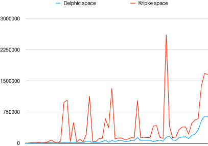
(a)

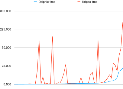
(b)

Figure 2: Results of the evaluation of the delphic and Kripke encodings.

We now analyze the results in detail. The central factor that contributes to the performance gains of delphic is the fact that possibilities allow for a more efficient use of space during the computation of a solution. Specifically, this efficiency results from two key aspects. First, as shown in Remark 1, possibility spectrums are able to represent epistemic information in a more compact way. Working with compact objects contributes significantly to reducing the size of epistemic states after sequences of updates. Second, as shown in Example 6, possibilities naturally allow to reuse previously calculated information (other possibilities that were calculated in previous states). We give a more concrete example of this property in Figure 3, that shows a sequence of epistemic states (surrounded by rectangles) from a generalization of the Coin in the Box domain of Example 1. We clearly see how the possibilities $\mathsf{w_{0}}$ and $\mathsf{w_{1}}$ are reused in the epistemic states $s_{1}$, $s_{2}$, $s_{3}$ and $s_{4}$. The space efficiency provided by delphic is clearly witnessed in Figure 2.a. In presence of instances with longer solutions, delphic outperforms the Kripke-based representation, as the latter requires a considerable amount of space to compute a solution (the spikes of the graph).

Figure 3: Reuse of previously calculated information in delphic. This figure was obtained by running the terminal command python delphic.py -i exp/CB/instance__pl_5.lp --print (see github.com/a-burigana/delphic_asp for the complete documentation).

The space efficiency of delphic is directly reflected on time performances. Indeed, in Figure 2.b are shown the same peaks in correspondence of instances with longer solutions. As a result, we can conclude that the delphic framework allows for a more scalable implementation both in terms of space and time performances. Finally, we point out that the analyzed performance gains are obtained in the average case, as there exist extreme (worst) cases where the two semantics produce epistemic states with the same structure. In fact, we recall that the delphic framework is semantically equivalent to the Kripke-based one (Theorem 3.1). Thus, we can conclude that delphic provides a practical and usable framework for DEL planning that can be exploited to tackle a wide range of concrete epistemic planning scenarios.

We close this section by noting that a similar, but less general result, was obtained by Fabiano et al. [11], where a possibility-based semantics is compared to the traditional Kripke-based one on a fragment of DEL called $m\mathcal{A}^{*}$ [4], that allows three kinds of actions, ontic, sensing and announcement actions. Since delphic is equivalent to the full DEL framework (see Theorem 3.1), our comparison indeed provides a generalization of the claim made by Fabiano et al.

5 Conclusions

We have introduced a novel epistemic planning framework, called delphic, based on the formal notion of possibility, in place of the more traditional Kripke-based DEL representation. We have formally shown that these two frameworks are semantically equivalent. Possibilities provide a more compact representation of epistemic states, in particular by reusing common information across states. To show the benefits of possibilities, we have implemented delphic and the Kripke-based approach in ASP, performing a comparative experimental evaluation with known benchmark domains. The results show that delphic indeed outperforms the Kripke-based approach both in terms of space and time performances, and is thus a good candidate for practical DEL planning.

In the future, we plan to exploit the performance gains provided by the delphic semantics in more competitive implementations based on C++. An interesting avenue of work is to deepen our analysis of possibility-based succinctness on fragments of DEL, where only a set of specific types of actions are allowed (the language $m\mathcal{A}^{*}$ [4] and the framework by Kominis and Geffner [15]).

Acknowledgements.

This research has been partially supported by the Italian Ministry of University and Research (MUR) under PRIN project PINPOINT Prot. 2020FNEB27, and by the Free University of Bozen-Bolzano with the ADAPTERS project.

Appendix 0.A Full Proofs

Lemma 2

Let $(\mathcal{E},E_{d})$ be an MPEM applicable in the MPKM $(M,W_{d})$, with solutions $\mathsf{E}$ and $\mathsf{W}$, respectively. Then the possibility spectrum $\mathsf{W^{\prime}}=\mathsf{W}\mathbin{\ooalign{$\cup$\cr\hfil\raise 1.80832pt\hbox{$\scriptscriptstyle\times$}\hfil\cr}}\mathsf{E}$ is the solution of $(M^{\prime},W^{\prime}_{d})=(M,W_{d})\otimes(\mathcal{E},E_{d})$.

Proof

Let $M=(W,R,V)$, $\mathcal{E}=(E,Q,pre,post)$ and $M^{\prime}=(W^{\prime},R^{\prime},V^{\prime})$. Let $\delta_{M}$ and $\delta_{\mathcal{E}}$ be the decorations for $M$ and $\mathcal{E}$, respectively. Let then $(\hat{M},\hat{W}_{d})$ be the picture of $\mathsf{W^{\prime}}$ via the decoration $\delta$, where $\hat{M}=(\hat{W},\hat{R},\hat{V})$. By Proposition 1, to prove that $\mathsf{W^{\prime}}$ is the solution of $(M^{\prime},W^{\prime}_{d})$, we need to show that $(M^{\prime},W^{\prime}_{d})\underline{\leftrightarrow}(\hat{M},\hat{W}_{d})$. Let $B\subseteq W^{\prime}\times\hat{W}$ be a relation such that:

$$(w^{\prime},\hat{w})\in B\Leftrightarrow w^{\prime}=(w,e)\wedge\delta(\hat{w})=\delta_{M}(w)\mathbin{\ooalign{$\cup$\cr\hfil\raise 1.80832pt\hbox{$\scriptscriptstyle\times$}\hfil\cr}}\delta_{\mathcal{E}}(e).$$

We now show that $B$ is a bisimulation between $M^{\prime}$ and $\hat{M}$. Let $(w^{\prime},\hat{w})\in B$, with $w^{\prime}=(w,e)$ and let $v^{\prime}=(v,f)\in W^{\prime}$. Let $\mathsf{w}=\delta_{M}(w)$, $\mathsf{e}=\delta_{\mathcal{E}}(e)$, $\mathsf{v}=\delta_{M}(v)$ and $\mathsf{f}=\delta_{\mathcal{E}}(f)$. Finally, let $\mathsf{w^{\prime}}=\mathsf{w}\mathbin{\ooalign{$\cup$\cr\hfil\raise 1.80832pt\hbox{$\scriptscriptstyle\times$}\hfil\cr}}\mathsf{e}=\delta(\hat{w})$ and $\mathsf{v^{\prime}}=\mathsf{v}\mathbin{\ooalign{$\cup$\cr\hfil\raise 1.80832pt\hbox{$\scriptscriptstyle\times$}\hfil\cr}}\mathsf{f}$.

• (Atom) Let $p\in\mathcal{P}$ be a propositional atom. Then:

  $w^{\prime}\in V^{\prime}(p)$	$\mathrel{\overset{\makebox[0.0pt]{\mbox{\tiny Def. 6}}}{\ \Leftrightarrow\ }}$	$(M,w)\models post(e)(p)$
  	$\mathrel{\overset{\makebox[0.0pt]{\mbox{\tiny Pr. 2, Def. 17}}}{\ \Leftrightarrow\ }}$	$\mathsf{w}\models\mathsf{e}(p)$
  	$\mathrel{\overset{\makebox[0.0pt]{\mbox{\tiny Def. 19}}}{\ \Leftrightarrow\ }}$	$\mathsf{w^{\prime}}(p)=1$
  	$\mathrel{\overset{\makebox[0.0pt]{\mbox{\tiny Def. 14}}}{\ \Leftrightarrow\ }}$	$\hat{w}\in\hat{V}(p)$

• (Forth/Back) Let $i\in\mathcal{AG}$ be an agent. Then:

  $w^{\prime}R^{\prime}_{i}v^{\prime}$	$\mathrel{\overset{\makebox[0.0pt]{\mbox{\tiny Def. 6}}}{\ \Leftrightarrow\ }}$	$wR_{i}v,eQ_{i}f,(M,w)\models pre(e)\text{ and }$
  		$(M,v)\models pre(f)$
  	$\mathrel{\overset{\makebox[0.0pt]{\mbox{\tiny Pr. 2, Def. 17}}}{\ \Leftrightarrow\ }}$	$\mathsf{v}\in\mathsf{w}(i),\mathsf{f}\in\mathsf{e}(i),\mathsf{w}\models\mathsf{e}(pre)\text{ and }$
  		$\mathsf{v}\models\mathsf{f}(pre)$
  	$\mathrel{\overset{\makebox[0.0pt]{\mbox{\tiny Def. 19}}}{\ \Leftrightarrow\ }}$	$\mathsf{v^{\prime}}\in\mathsf{w}^{\prime}(i)$
  	$\mathrel{\overset{\makebox[0.0pt]{\mbox{\tiny Def. 14}}}{\ \Leftrightarrow\ }}$	$\hat{w}\hat{R}_{i}\hat{v}$

• (Designated) Let $(w^{\prime}_{d},\hat{w}_{d})\in B$, with $w^{\prime}_{d}=(w,e)$. Then:

  $w^{\prime}_{d}{\in}W^{\prime}_{d}$	$\mathrel{\overset{\makebox[0.0pt]{\mbox{\tiny Def. 6}}}{\ \Leftrightarrow\ }}$	$w{\in}W_{d},e{\in}E_{d}\text{ and }(M,w){\models}pre(e)$
  	$\mathrel{\overset{\makebox[0.0pt]{\mbox{\tiny Pr. 2, Def. 17}}}{\ \Leftrightarrow\ }}$	$\mathsf{w}\in\mathsf{W},\mathsf{e}\in\mathsf{E}\text{ and }\mathsf{w}\models\mathsf{e}(pre)$
  	$\mathrel{\overset{\makebox[0.0pt]{\mbox{\tiny Def. 19}}}{\ \Leftrightarrow\ }}$	$\mathsf{w^{\prime}}\in\mathsf{W^{\prime}}$
  	$\mathrel{\overset{\makebox[0.0pt]{\mbox{\tiny Def. 14}}}{\ \Leftrightarrow\ }}$	$\hat{w}_{d}\in\hat{W}_{d}$

Appendix 0.B ASP Encodings

In this section, we describes the Answer Set Programming (ASP) encodings of delphic and of the traditional Kripke semantics for DEL. We assume that the reader is familiar with the basics concepts of ASP. Notably, our encodings make use of the multi-shot solving strategy provided by the ASP-solver clingo, which provides fine-grained control over grounding and solving of ASP programs, and is instrumental to implementing an incremental strategy for solving. For a detailed introduction on multi-shot ASP solving, we refer the reader to [12, 14].

We developed our ASP encodings in such a way that delphic objects (possibility/eventuality spectrums) and DEL objects (MPKMs/MPEMs) are encoded by closely mirroring each other, and only differing in the two update operators (union update and product update). This homogeneity is instrumental to obtain a fair experimental comparison of the two encodings, presented in Section 4 of the main paper. At the same time, as detailed later, we stress that the timings exhibited by our ASP encoding of the Kripke semantics are comparable to those shown by the state-of-the-art solver EFP 2.0 [11], which also implements on the Kripke semantics. Due to the similarity of the two encodings, in the following we use generic terms such as “epistemic state/action” and “planning task” to abstract away from which underlying semantics is actually chosen.

The delphic encoding presented in this section constitutes a contribution of this paper of independent interest. In fact, it generalizes the ASP-based epistemic planner PLATO [8], which implements a possibility-based semantics for a fragment of DEL [11]. Moreover, having an ASP-based solver for epistemic planning has several benefits. First, the declarative encoding of the delphic semantics allows for an implementation that is transparent and easier to inspect. Second, we exploited the Python API offered by clingo to implement a graphical representation that shows the epistemic states visited by the planner. We thus obtain a practical and useful tool that allows to visualize the evolution of the system. This feature is instrumental in different tasks, such as designing new epistemic planning domains and debugging the correctness of implementations. We concretely show a graphical comparison of the output of the two encodings in the appendix on a concrete domain instance (we do not directly report it here due to space reasons).

The remainder of the section is as follows. First, we briefly describe how incremental solving is achieved by the multi-shot solving technique (Section 0.B.1). Then, we illustrate both encodings component by component: (i) formulae in Section 0.B.2, (ii) planning tasks in Section 0.B.3, (iii) epistemic states in Section 0.B.4, (iv) truth conditions in Section 0.B.5, and (v) update operators in Section 0.B.6).

0.B.1 Multi-shot Encoding

The multi-shot approach allows one to divide an ASP encoding into sub-programs, then handling grounding and solving of these sub-programs separately. In particular, this technique is useful to implement incremental solving, which, at each time step, allows to extend the ASP program in order to look for solutions of increasing size. Intuitively, every step mimics a Breadth-First Search over the planning state space: at each time step $\mathtt{t}$, if a solution is not found (there is no plan of length $\mathtt{t}$ that satisfies the goal), the ASP program is expanded to look for a longer plan.

To achieve incremental solving, we build on the approach by Gebser et al. [12], splitting our encodings in three subprograms: 1. program $\mathtt{base}$, which contains all the static information (input information on the planning task); 2. program $\mathtt{step(t)}$, where $\mathtt{t}{>}0$, which describes the evolution of the system (updates semantics); and 3. program $\mathtt{check(t)}$, where $\mathtt{t}{\geq}0$, which verify the truth of formulae of the domain and, in particular, of the goal formula. Here, $\mathtt{t}$ represents the current time step that is being considered. In the reminder of this section, when we describe components of the encodings pertaining to the sub-programs $\mathtt{step(t)}$ and $\mathtt{check(t)}$, we assume $\mathtt{t}$ fixed.

0.B.2 Formulae

We represent epistemic formulae through nested ASP predicates. To enhance the performance of grounding and solving, we assume that all input formulae are given in a normal form where occurrences of the $\Box_{i}$ operators are replaced by the dual representation $\neg\Diamond_{i}\neg$, and where double negation is simplified. Agents and atoms are represented by the ASP predicates $\mathtt{agent(AG)}$ and $\mathtt{atom(P)}$, respectively. A formula $\varphi$ is encoded inductively on its structure: 1. $\varphi=p$is encoded by $\mathtt{p}$; 2. $\varphi=\neg\psi$is encoded by $\mathtt{neg(PSI)}$; 3. $\varphi=\psi_{1}\wedge\psi_{2}$is encoded by $\mathtt{and(PSI_{1},PSI_{2})}$; and 4. $\varphi=\Diamond_{i}\psi$is encoded by $\mathtt{dia(i,PSI)}$.

0.B.3 Planning Tasks

We now describe our ASP encoding of a planning task.

Initial State. The initial state is given by the following ASP predicates: 1. $\mathtt{w\_init(W)}$: $\mathtt{W}$ is an initial possibility/possible world; 2. $\mathtt{r\_init(W_{1},W_{2},AG)}$: in $\mathtt{W_{1}}$, agent $\mathtt{AG}$ considers $\mathtt{W_{2}}$ to be possible; 3. $\mathtt{v\_init(W,P)}$: atom $\mathtt{P}$ is true in $\mathtt{W}$; 4. $\mathtt{dw\_init(W)}$: $\mathtt{W}$ is a designated possibility/world.

Actions. To obtain efficient encodings of the two semantics, and directly support existing benchmarks from the literature, we introduce two features in the definition of actions, namely (global) action preconditions and observability conditions.

An action precondition is specified with the ASP predicate $\mathtt{action\_pre(ACT,PRE)}$ and represents the applicability of the action as a whole. This is syntactic sugar: action preconditions do not modify the expressiveness of epistemic actions, and one can always get an equivalent epistemic action that does not employ them.

Observability conditions provide a useful way to compactly represent epistemic actions. Namely, agents are split into observability groups classifying different perspectives of agents w.r.t. an action. For instance, in Example 2, agent $a$ is fully observant, since it is the one that performs the action, whereas agent $b$ is oblivious, since it does not know that the action is taking place. Then, as we show below, the information regarding which eventuality/event are considered to be possible is lifted to observability groups. Each action must then specify the observability conditions for each agent, assigning each agent to an observability group. This strategy yields an much more succinct representation since each action needs to be substantiated for each group combination, rather than for each agent combination.

We are now ready to describe the ASP encoding of an action $\mathtt{ACT}$: 1. $\mathtt{e(ACT,E)}$: $\mathtt{E}$ is an eventuality/event of $\mathtt{ACT}$; 2. $\mathtt{q(ACT,E_{1},E_{2},GR)}$: in $\mathtt{E_{1}}$, the observability group $\mathtt{GR}$ considers $\mathtt{E_{2}}$ to be possible; 3. $\mathtt{obs(ACT,AG,GR,COND)}$: agent $\mathtt{AG}$ is in the observability group $\mathtt{GR}$ if the condition $\mathtt{COND}$ is satisfied by the current epistemic state; 4. $\mathtt{pre(ACT,E,PRE)}$: the precondition of $\mathtt{E}$ is $\mathtt{PRE}$; 5. $\mathtt{post(ACT,E,P,POST)}$: the postcondition of $\mathtt{P}$ in $\mathtt{E}$ is $\mathtt{POST}$; 6. $\mathtt{de(ACT,E)}$: $\mathtt{E}$ is a designated eventuality/event of $\mathtt{ACT}$.

We also define some auxiliary ASP predicates that will be used in the update encodings (Section 0.B.6), namely $\mathtt{idle(ACT,E)}$ and $\mathtt{inertia(ACT,E,P)}$, which are calculated at the beginning of the ASP computation. The former predicate states that $\mathtt{E}$ does not affect the worlds in any way ($e_{2}$ in Example 2 is idle). The latter predicate states that atom $\mathtt{P}$ is not changed by the postconditions of $\mathtt{E}$.

Goal. The goal of a planning task is represented by the ASP $\mathtt{goal(F)}$ predicates. It is possible to declare multiple goal formulae, so that the goal condition of the planning task is the conjunction of all these $\mathtt{goal}$ predicates.

0.B.4 Epistemic States

The components of an epistemic state that must be represented (in delphic as well as in the traditional DEL semantics) are four: (i) possibilities/possible worlds; (ii) information states/accessibility relations; (iii) valuation of propositional atoms; (iv) designated possibilities/worlds.

Possibilities and Possible Worlds. To describe possibilities and possible worlds, we make use of the ASP predicate $\mathtt{w(t,W,E)}$. A possibility/world needs three variable to be univocally identified:

• $\mathtt{t}$: represents the time instant when the possibility/world was created. In the initial state, the time is set to $\mathtt{0}$;

• $\mathtt{W}$: represents the possibility/world that is being updated;

• $\mathtt{E}$: represents the eventuality/event that is updating $\mathtt{W}$.

As at planning time new possibilities/worlds are created dynamically, we are faced with the challenge of finding a suitable ASP representation that correctly and univocally encodes the worlds that are being updated during each action. This is best explained with an example. Suppose we update the possibility/world $\mathtt{w(t{-}1,W,E)}$ with the eventuality/event $\mathtt{e(ACT,F)}$ and let $\mathtt{w(t,X,F)}$ be the result of the update. Intuitively, we can see $\mathtt{X}$ as representing the world being updated ($\mathtt{w(t{-}1,W,E)}$). Thus, the challenge we are facing here is to find a suitable representation for $\mathtt{X}$.

On the one hand, when encoding possibilities, we have to bear in mind that at each time step, we might end up updating possibilities that were previously calculated at any time in the past. As a result, to correctly and univocally encode $\mathtt{X}$, we need to keep track of the following information: (i) the time when a possibility was created; (ii) the identifier of the possibility; and (iii) the eventuality that created it. As a result, we represent $\mathtt{X}$ as the ASP tuple $\mathtt{(t{-}1,W,E)}$.

On the other hand, when encoding possible worlds, we can always be sure that at each time step we are updating worlds that were created at precisely that time. Thus, the ASP encoding of a possible world is slightly simplified and we represent $\mathtt{X}$ with the ASP tuple $\mathtt{(W,E)}$.

Finally, the initial possibilities/worlds are calculated from the initial state representation with the ASP rule $\mathtt{w(0,W,null)}$ :- $\mathtt{w\_init(W).}$, where $\mathtt{null}$ is a placeholder that indicates that no action occurred before time $\mathtt{t}$.

Example 7

The possibilities of Example 6 are represented in ASP as follows: (i) $\mathsf{w_{1}}$: $\mathtt{w(0,w_{1},null)}$; (ii) $\mathsf{w_{2}}$: $\mathtt{w(0,w_{2},null)}$; and (iii) $\mathsf{v_{3}}$: $\mathtt{w(1,(0,w_{1},null),e_{1})}$. Again, notice that, in the ASP encoding of possibilities, we are able to reuse previously calculated information.

Similarly, the possible worlds of Example 3 are represented in ASP as: (i) $v_{1}$: $\mathtt{w(1,(w_{1},null),e_{2})}$; (ii) $v_{2}$: $\mathtt{w(1,(w_{2},null),e_{2})}$; and (iii) $v_{3}$: $\mathtt{w(1,(w_{1},null),e_{1})}$.

Information States and Accessibility Relations. Let $\mathtt{w(Tw,W,Ew)}$ and $\mathtt{w(Tv,V,Ev)}$ be the ASP representations of two possibilities $\mathsf{w}$ and $\mathsf{v}$. Since the possibilities contained in the information states of $\mathsf{w}$ might have been calculated at any time step in the past, in order to encode the fact that $\mathsf{v}\in\mathsf{w}(i)$ (where $i\in\mathcal{AG}$), we need to keep track of the time when $\mathsf{v}$ was created. As a result, the resulting encoding is given by the ASP predicate $\mathtt{r(Tw,W,Ew,Tv,V,Ev,I)}$.

Let now $\mathtt{w(Tw,W,Ew)}$ and $\mathtt{w(Tv,V,Ev)}$ refer to two possible worlds $w$ and $v$. When representing accessibility relations, we can always be sure that when $wR_{i}v$, the ASP representation of the worlds $w$ and $v$ share the same time value ($\mathtt{Tw=Tv}$). Thus, we can simplify the encoding as follows: $\mathtt{r(Tw,W,Ew,V,Ev,I)}$.

Example 8

The information states of Example 6 are represented in ASP as follows (we do not further expand the information states of $\mathsf{w_{1}}$ and $\mathsf{w_{2}}$ as they refer to previously calculated information):

• $\mathsf{v_{3}}{\in}\mathsf{v_{3}}(a)$: $\mathtt{r(1,(0,w_{1},null),e_{1},1,(0,w_{1},null),e_{1},a)}$;

• $\mathsf{w_{1}}{\in}\mathsf{v_{3}}(b)$: $\mathtt{r(1,(0,w_{1},null),e_{1},0,w_{1},null,b)}$; and

• $\mathsf{w_{2}}{\in}\mathsf{v_{3}}(b)$: $\mathtt{r(1,(0,w_{1},null),e_{1},0,w_{2},null,b)}$.

The accessibility relations of Example 3 are represented in ASP as follows:

• $v_{3}R_{a}v_{3}$: $\mathtt{r(1,(w_{1},null),e_{1},(w_{1},null),e_{1},a)}$;

• $v_{3}R_{b}v_{1}$: $\mathtt{r(1,(w_{1},null),e_{1},(w_{1},null),e_{2},b)}$;

• $v_{3}R_{b}v_{2}$: $\mathtt{r(1,(w_{1},null),e_{1},(w_{2},null),e_{2},b)}$; and

• $v_{x}R_{i}v_{y}$: $\mathtt{r(1,(w_{x},null),e_{2},(w_{y},null),e_{2},i)}$, for each $x,y\in\{1,2\}$ and $i\in\{a,b\}$.

Valuations. For each atom $\mathtt{P}$, we encode the fact that $\mathtt{P}$ is true in the possibility/world $\mathtt{w(t,W,E)}$ with the ASP predicate $\mathtt{v(t,W,E,P)}$. We only represent true atoms. The initial valuation is calculated from the initial state representation with the ASP rule $\mathtt{v(0,W,null,P)}$ :- $\mathtt{v\_init(W,P)}$.

Designated Possibilities and Worlds. A designated possibility/world is represented by the ASP predicate $\mathtt{dw(t,W,E)}$, where variables $\mathtt{t}$, $\mathtt{W}$ and $\mathtt{E}$ have the same meaning as in $\mathtt{w(t,W,E)}$. The initial designated possibilities/worlds are calculated from the initial state representation with the ASP rule $\mathtt{dw(0,W,null)}$ :- $\mathtt{dw\_init(W)}$.

0.B.5 Truth Conditions

For space constraints, we abbreviate the representation $\mathtt{Tx,X,Ex}$ of a possibility/world as $\mathtt{\bar{X}}$. Truth conditions of formulae are encoded by predicate $\mathtt{holds(t,W,E,F)}$, defined by induction on the structure of formulae as follows:

$\mathtt{holds(\bar{W},P)}$	:-  $\mathtt{v(\bar{W},P),atom(P).}$
$\mathtt{holds(\bar{W},neg(F))}$	:-  $\mathtt{not\ holds(\bar{W},F).}$
$\mathtt{holds(\bar{W},and(F_{1},F_{2}))}$	:-  $\mathtt{holds(\bar{W},F_{1}),holds(\bar{W},F_{2}).}$
$\mathtt{holds(\bar{W},dia(AG,F))}$	:-  $\mathtt{r(\bar{W},\bar{V},AG),holds(\bar{V},F).}$

0.B.6 Update Operators

We now describe the ASP encodings of the update operators. As the encodings differ, we present them individually.

Union Update. Let the ASP representations of a possibility spectrum $\mathsf{W}$ at time $\mathtt{t}$ and of an eventuality spectrum $\mathsf{ACT}$ be given. We now show how the encoding of the update $\mathsf{W^{\prime}}=\mathsf{W}\mathbin{\ooalign{$\cup$\cr\hfil\raise 1.80832pt\hbox{$\scriptscriptstyle\times$}\hfil\cr}}\mathsf{E}$ is obtained. We adopt again the short representation for possibilities/worlds ($\mathtt{\bar{X}}$). We point out that the following ASP rules have a one-to-one correspondence with Definition 19. First, the designated possibilities of $\mathsf{W^{\prime}}$ are determined by the following ASP rules:

$\mathtt{dw(t,\bar{W},E)}$	:-	$\mathtt{dw(\bar{W}),de(ACT,E),pre(ACT,E,PRE),}$
		$\mathtt{holds(\bar{W},PRE).}$

To describe how possibilities are updated, we need the following ASP predicate:

$\mathtt{qt(t,E,F,I)}$

:-

$\mathtt{q(ACT,E,F,GR),obs(t,I,GR).}$

That is, we evaluate the observability conditions of each agent to determine the information states of the action. From this, we can obtain all the updated possibilities recursively:

$\mathtt{w(t,\bar{W},E)}$	:-	$\mathtt{dw(t,\bar{W},E),de(ACT,E).}$
$\mathtt{w(t,\bar{W},E)}$	:-	$\mathtt{w(t,\bar{V},F),pre(ACT,E,PRE),\textnormal{-}idle(ACT,E),}$
		$\mathtt{r(\bar{V},\bar{W},I),qt(t,F,E,I),holds(\bar{W},PRE).}$

The first rule states that a designated possibility is a possibility. Let now $\mathsf{v^{\prime}}=\mathsf{v}\mathbin{\ooalign{$\cup$\cr\hfil\raise 1.80832pt\hbox{$\scriptscriptstyle\times$}\hfil\cr}}\mathsf{f}$. Then, the second rule states that for any $\mathsf{w}$ and $\mathsf{e}$ such that $\mathsf{w}\in\mathsf{v}(i)$, $\mathsf{e}\in\mathsf{f}(i)$ and $\mathsf{w}\models\mathsf{e}(pre)$, we create $\mathsf{w^{\prime}}=\mathsf{w}\mathbin{\ooalign{$\cup$\cr\hfil\raise 1.80832pt\hbox{$\scriptscriptstyle\times$}\hfil\cr}}\mathsf{e}$. Notice that we require that the eventuality $\mathsf{e}$ is not idle. An eventuality/event is idle when its precondition is $\top$ and when its postconditions are the identity function. In this way, we do not copy redundant information.

Let now $\mathtt{\bar{W}^{\prime}}$ and $\mathtt{\bar{V}^{\prime}}$ stand for $\mathtt{t,\bar{W},E}$ and $\mathtt{t,\bar{V},F}$, respectively, and let $\mathtt{\bar{U}}$ stand for $\mathtt{Tu,\bar{U},Eu}$. We encode information states as follows:

$\mathtt{r(\bar{W}^{\prime},\bar{V}^{\prime},I)}$	:-	$\mathtt{r(\bar{W},\bar{V},I),qt(t,E,F,I).}$
$\mathtt{r(\bar{W}^{\prime},\bar{U},\leavevmode\nobreak\ I)}$	:-	$\mathtt{r(\bar{W},\bar{U},I),qt(t,E,F,I),Tu{\leq}t,idle(ACT,F).}$

The first rule states that if $\mathsf{w^{\prime}}=\mathsf{w}\mathbin{\ooalign{$\cup$\cr\hfil\raise 1.80832pt\hbox{$\scriptscriptstyle\times$}\hfil\cr}}\mathsf{e}$ and $\mathsf{v^{\prime}}=\mathsf{v}\mathbin{\ooalign{$\cup$\cr\hfil\raise 1.80832pt\hbox{$\scriptscriptstyle\times$}\hfil\cr}}\mathsf{f}$ are both created at time $\mathtt{t}$ and it holds that $\mathsf{v}\in\mathsf{w}(i)$ and $\mathsf{f}\in\mathsf{e}(i)$, then $\mathsf{v^{\prime}}\in\mathsf{w^{\prime}}(i)$. The second rule states that if $\mathsf{w^{\prime}}=\mathsf{w}\mathbin{\ooalign{$\cup$\cr\hfil\raise 1.80832pt\hbox{$\scriptscriptstyle\times$}\hfil\cr}}\mathsf{e}$ is created at time $\mathtt{t}$ and it holds that $\mathsf{u}\in\mathsf{w}(i)$ and there exists an eventuality $\mathsf{f}$ such that $\mathsf{f}\in\mathsf{e}(i)$ and $\mathsf{u}=\mathsf{u}\mathbin{\ooalign{$\cup$\cr\hfil\raise 1.80832pt\hbox{$\scriptscriptstyle\times$}\hfil\cr}}\mathsf{f}$, then $\mathsf{u}\in\mathsf{w^{\prime}}(i)$. In this way, we are able to reuse previously calculated information when encoding information states of possibilities.

Finally, we encode the valuation of atoms as follows:

$\mathtt{v(\bar{W}^{\prime},P)}$	:-	$\mathtt{post(ACT,E,P,POST),holds(\bar{W},POST).}$
$\mathtt{v(\bar{W}^{\prime},P)}$	:-	$\mathtt{inertia(ACT,E,P),v(\bar{W},P).}$

The first rule states that if $\mathsf{w}\models\mathsf{e}(p)$, then $\mathsf{w^{\prime}}(p){=}1$. The second rule states that if there are no postconditions associated to an atom (represented by the ASP predicate $\mathtt{inertia}$), then in $\mathsf{w^{\prime}}$ we keep the truth value assigned to $p$ in $\mathsf{w}$.

Product Update. Let the ASP representations of a MPKM $(M,W_{d})$ at time $\mathtt{t}$ and of a MPEM $(\mathcal{E},E_{d})$ be given. The following ASP rules have a one-to-one correspondence with Definition 6. Designated worlds and valuation of atoms are defined in the same way as in the previous case. As above, let $\mathtt{\bar{W}^{\prime}}$ and $\mathtt{\bar{V}^{\prime}}$ stand for $\mathtt{t,\bar{W},E}$ and $\mathtt{t,\bar{V},F}$, respectively. Then, updated possible worlds and accessibility relations are encoded as:

$\mathtt{w(t,\bar{W},E)}$	:-	$\mathtt{w(\bar{W}),e(ACT,E),holds(\bar{W},PRE).}$
$\mathtt{r(\bar{W}^{\prime},\bar{V}^{\prime},I)}$	:-	$\mathtt{r(\bar{W},\bar{V},I),qt(t,E,F,I).}$

0.B.7 Epistemic Planning Domains

We overview the planning domains used for the evaluation.

Assemble Line (AL): there are two agents, each responsible for processing a different part of a product. Each agent can fail in processing its part and can inform the other agent of the status of her task. The agents can decide to assemble the product or to restart the process, depending on their knowledge about the product status. This domain is parametrized on the maximum modal depth $d$ of formulae that appear in the action descriptions. The goal in this domain is fixed, the agents must assemble the product. The aim of this domain is to analyze the impact of the modal depth both in terms of grounding and solving performances.

Coin in the Box (CB): this is a generalization of the domain presented in Example 1. Three agents are in a room where a closed box contains a coin. None of them knows whether the coin lies heads or tails up. To look at the coin, the agents need to first open the box. Agents can be attentive or distracted: only attentive agents are able to see what actions are executed. Moreover, agents can signal others to make them attentive and can also distract them. The goal is for one or more agents to learn the coin position.

Collaboration and Communication (CC): $n{\geq}2$ agents move along a corridor with $k{\geq}2$ rooms in which $m{\geq}1$ boxes are located. Whenever an agent enters a room, it can determine whether a box is there. Agents can then communicate information about the position of the boxes to each other. The goal is to have some agent learn the position of one or more boxes and to know what other agents have learnt.

Grapevine (Gr): $n{\geq}2$ agents can move along a corridor with $2$ rooms and share their own “secret” to agents in the same room. The goal requires agents to know the secret of one or more agents and to hide their secret to others.

Selective Communication (SC): $n{\geq}2$ agents can move along a corridor with $k{\geq}2$ rooms. The agents might share some information, represented by an atom $q$. In each room, only a certain subset of agents is able to listen to what others share. The goal requires for some specific subset of agents to know the information and to hide it to others.

Appendix 0.C Graphical Comparison

We briefly report a concrete example on the succinctness of the possibility-based representation, compared to the Kripke-based one (Figures 4 and 5). The figures were generated by our tool. As you can see, even for small plans of length 5, the delphic semantics provide a much more succinct representation. Specifically, in Figure 4 we obtain a total of 15 possibilities, while in Figure 5 we obtain 126 possible worlds. This clearly confirms the benefits of the delphic semantics.

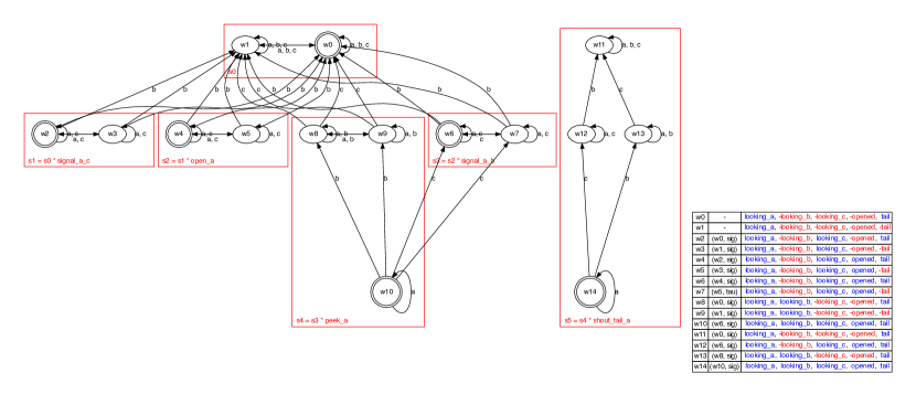
Figure 4: Graphical representation of a sequence of 5 actions using delphic.

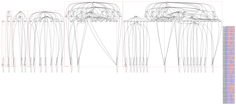
Figure 5: Graphical representation of a sequence of 5 actions using Kripke semantics.

Appendix 0.D Full Experimental Results

We here report the complete tables with the results of our experimental evaluations (Tables 1-5).

Assemble
$|\mathcal{AG}|$	$|\mathcal{P}|$	$|W|$	$|\mathcal{A}|$	$L$	$d$	Delphic		Kripke
						Time	Atoms	Time	Atoms
2	4	4	6	5	2	2.560	59332	3.153	123780
					3	2.621	60390	3.606	121194
					4	2.913	61422	4.396	128644
					5	3.117	62478	4.148	125708
					6	3.304	63564	4.774	128328
					7	3.410	64622	4.917	130464
					8	3.372	65680	5.556	138372
					9	3.566	66738	6.161	140804
					10	3.739	67796	6.888	136576
					24	13.103	108000	25.264	218362

Table 1: Results for AL.

Coin in the Box
$|\mathcal{AG}|$	$|\mathcal{P}|$	$|W|$	$|\mathcal{A}|$	$L$	$d$	delphic		Kripke
						Time	Atoms	Time	Atoms
3	5	2	21	2	1	0.077	2459	0.098	3094
				3	1	0.215	5828	0.231	8394
				5	3	5.137	77310	7.014	122265
				6	3	27.428	316840	54.091	586037
				7	3	t.o.	-	t.o.	-

Table 2: Results for CB.

Collaboration and Communication
$|\mathcal{AG}|$	$|\mathcal{P}|$	$|W|$	$|\mathcal{A}|$	$L$	$d$	Delphic		Kripke
						Time	Atoms	Time	Atoms
2	10	4	20	3	2	0.129	4579	0.186	8859
				4	1	0.455	10900	0.532	25916
				5	2	2.467	37882	3.599	98226
				6	2	9.435	147183	25.365	385343
				7	2	66.278	636799	254.544	1652783
				8	2	t.o.	-	t.o.	-
3	13	4	30	3	2	0.167	7112	0.328	13532
				4	1	0.774	15873	0.958	37125
				5	2	5.580	57033	9.321	147549
				6	2	18.550	214086	78.667	557746
				7	2	143.178	934859	t.o.	-
				8	2	t.o.	-	t.o.	-
3	15	8	42	3	2	0.905	17288	1.153	36040
				4	1	3.939	46741	4.392	114453
				5	2	14.207	184241	85.423	477169
				6	2	114.014	760234	465.422	1963514
				7	2	t.o.	-	t.o.	-
				8	2	t.o.	-	t.o.	-
2	14	9	28	3	2	0.541	13456	0.723	28514
				4	1	2.778	39077	3.020	96399
				5	2	12.418	152271	38.747	393337
				6	2	57.073	650494	146.581	1681652
				7	2	t.o.	-	t.o.	-
2	17	18	40	3	2	2.688	39310	3.324	87272
				4	1	7.849	128993	14.633	322395
				5	2	52.642	535713	115.531	1376539
				6	2	t.o.	-	t.o.	-
				7	2	t.o.	-	t.o.	-

Table 3: Results for CC.

Grapevine
$|\mathcal{AG}|$	$|\mathcal{P}|$	$|W|$	$|\mathcal{A}|$	$L$	$d$	Delphic		Kripke
						Time	Atoms	Time	Atoms
3	9	8	24	2	1	0.104	3644	0.165	9256
				3	1	0.197	5385	0.892	28491
				4	1	0.500	9294	4.142	98558
				5	1	1.934	18691	44.456	372271
				6	2	15.943	43315	t.o.	-
				7	2	52.829	107146	t.o.	-
4	12	16	40	2	1	0.360	10684	0.810	32104
				3	1	1.096	17182	6.613	109032
				4	1	3.694	33024	41.454	412426
				5	1	15.049	73698	t.o.	-
				6	2	87.727	184055	t.o.	-
				7	2	t.o.	-	t.o.	-
5	15	32	60	2	1	1.153	33600	4.593	113362
				3	1	3.695	58527	48.582	417771
				4	1	9.469	123422	t.o.	-
				5	1	77.333	298973	t.o.	-
				6	2	t.o.	-	t.o.	-
				7	2	t.o.	-	t.o.	-

Table 4: Results for Gr.

Selective Communication
$|\mathcal{AG}|$	$|\mathcal{P}|$	$|W|$	$|\mathcal{A}|$	$L$	$d$	Delphic		Kripke
						Time	Atoms	Time	Atoms
3	5	2	7	3	2	0.026	943	0.029	1848
				5	1	0.111	5451	0.354	18231
				6	3	0.190	7775	1.948	74916
				8	3	2.063	62367	81.041	1318062
7	5	2	7	5	1	0.188	11342	0.545	30615
				7	2	1.778	67906	20.629	579934
				8	2	4.192	140081	179.118	2617071
8	11	2	13	9	1	0.236	10156	52.347	976904
				10	2	0.339	14519	178.486	1036341
				14	2	17.766	494657	t.o.	-
				15	2	16.430	481155	t.o.	-
9	11	2	13	6	2	4.542	167342	9.196	414842
				8	2	27.503	653357	t.o.	-
				9	2	94.207	1693676	t.o.	-
				12	2	t.o.	-	t.o.	-
9	11	2	13	9	2	0.373	21893	29.649	494173
				10	2	0.723	41257	195.693	1135358
				13	2	1.989	95485	t.o.	-
				17	2	288.827	4023556	t.o.	-
9	12	2	14	4	1	0.084	4712	0.143	12602
				5	1	0.234	15034	0.848	49580
				6	1	0.678	43058	3.560	212899
				7	1	3.165	132163	27.126	1030477
				8	1	15.983	393797	t.o.	-
				9	1	32.373	782700	t.o.	-
				10	1	129.964	2458577	t.o.	-
				11	1	289.298	4209828	t.o.	-

Table 5: Results for SC.

References

- [1] Aczel, P.: Non-well-founded sets, CSLI lecture notes series, vol. 14. CSLI (1988)
- [2] Aucher, G., Bolander, T.: Undecidability in epistemic planning. In: Rossi, F. (ed.) IJCAI 2013, Proceedings of the 23rd International Joint Conference on Artificial Intelligence, Beijing, China, August 3-9, 2013. pp. 27–33. IJCAI/AAAI (2013)
- [3] Baltag, A., Moss, L.S., Solecki, S.: The logic of public announcements and common knowledge and private suspicions. In: Gilboa, I. (ed.) Proceedings of the 7th Conference on Theoretical Aspects of Rationality and Knowledge (TARK-98), Evanston, IL, USA, July 22-24, 1998. pp. 43–56. Morgan Kaufmann (1998)
- [4] Baral, C., Gelfond, G., Pontelli, E., Son, T.C.: An action language for multi-agent domains: Foundations. CoRR abs/1511.01960 (2015)
- [5] Bolander, T., Andersen, M.B.: Epistemic planning for single and multi-agent systems. J. Appl. Non Class. Logics 21(1), 9–34 (2011)
- [6] Bolander, T., Charrier, T., Pinchinat, S., Schwarzentruber, F.: Del-based epistemic planning: Decidability and complexity. Artif. Intell. 287, 103304 (2020)
- [7] Bolander, T., Dissing, L., Herrmann, N.: DEL-based Epistemic Planning for Human-Robot Collaboration: Theory and Implementation. In: Proceedings of the 18th International Conference on Principles of Knowledge Representation and Reasoning. pp. 120–129 (11 2021)
- [8] Burigana, A., Fabiano, F., Dovier, A., Pontelli, E.: Modelling multi-agent epistemic planning in ASP. Theory Pract. Log. Program. 20(5), 593–608 (2020)
- [9] van Ditmarsch, H., Kooi, B.: Semantic results for ontic and epistemic change, pp. 87–117. Texts in Logic and Games 3, Amsterdam University Press (2008)
- [10] van Ditmarsch, H.P., van der Hoek, W., Kooi, B.P.: Dynamic Epistemic Logic, vol. 337. Springer Netherlands (2007)
- [11] Fabiano, F., Burigana, A., Dovier, A., Pontelli, E.: EFP 2.0: A multi-agent epistemic solver with multiple e-state representations. In: Beck, J.C., Buffet, O., Hoffmann, J., Karpas, E., Sohrabi, S. (eds.) Proceedings of the Thirtieth International Conference on Automated Planning and Scheduling, Nancy, France, October 26-30, 2020. pp. 101–109. AAAI Press (2020)
- [12] Gebser, M., Kaminski, R., Kaufmann, B., Schaub, T.: Multi-shot ASP solving with clingo. Theory Pract. Log. Program. 19(1), 27–82 (2019)
- [13] Gerbrandy, J., Groeneveld, W.: Reasoning about information change. J. Log. Lang. Inf. 6(2), 147–169 (1997)
- [14] Kaminski, R., Romero, J., Schaub, T., Wanko, P.: How to build your own asp-based system?! Theory Pract. Log. Program. 23(1), 299–361 (2023)
- [15] Kominis, F., Geffner, H.: Beliefs in multiagent planning: From one agent to many. In: Brafman, R.I., Domshlak, C., Haslum, P., Zilberstein, S. (eds.) Proceedings of the Twenty-Fifth International Conference on Automated Planning and Scheduling, ICAPS 2015, Jerusalem, Israel, June 7-11, 2015. pp. 147–155. AAAI Press (2015)
- [16] Kripke, S.A.: Semantical considerations on modal logic. Acta Philosophica Fennica 16(1963), 83–94 (1963)