On a moment generalization of some classical second-order differential equations generating classical orthogonal polynomials

Abstract

The aim of the work is to construct new polynomial systems, which are solutions to certain functional equations which generalize the second-order differential equations satisfied by the so called classical orthogonal polynomial families of Jacobi, Laguerre, Hermite and Bessel. These functional equations can be chosen to be of different type: fractional differential equations, q-difference equations, etc, which converge to their respective differential equations of the aforesaid classical orthogonal polynomials. In addition to this, there exists a confluence of both the families of polynomials constructed and the functional equations who approach to the classical families of polynomials and second-order differential equations, respectively

Key words: moment sequence, formal solution, q-difference equation, fractional differential equation. 2020 MSC: 33C45, 11B83, 30D05, 34K05, 34K37

1 Introduction

An infinite sequence of polynomials $(\varphi_{n}(x))_{n\geq 0}$ with $\hbox{deg}(\varphi_{n}(x))=n$, is said to be orthogonal with respect to certain positive Borel measure $\mu$ supported in an infinite set $E\subseteq\mathbb{R}$, if all the following quantities, known as their moments, satisfy

$$\int_{E}x^{n}d\mu(x)<\infty,\quad n\in\mathbb{N}_{0}:=\{0,1,\ldots\},$$

and the polynomials in the sequence fulfill

$$\int_{E}\varphi_{m}(x)\varphi_{n}(x)d\mu(x)=\xi_{n}\delta_{m,n},\quad m,n\in\mathbb{N}_{0},$$

where $\delta_{m,n}$ stands for the Kronecker delta (i.e. $\delta_{m,n}=0$ for $m\neq n$ and $\delta_{n,n}=1$), and where $\xi_{n}$ is a positive real number for all $n\in\mathbb{N}_{0}$ (see, for example [6, 7, 24]).

Said polynomial sequence $(\varphi_{n}(x))_{n\geq 0}$ is also called classical, if there exist a polynomial of degree at most 2, say $\sigma=\sigma(x)$ and a polynomial of degree at most one, say $\tau=\tau(x)$, such that for every $n\in\mathbb{N}_{0}$ a real constant $\lambda_{n}$ exists for which $\varphi_{n}(x)$ satisfies the second-order differential equation

(1) $$\sigma(x)y^{\prime\prime}(x)+\tau(x)y^{\prime}(x)+\lambda_{n}y(x)=0.$$

Observe that the restriction on the degree of the polynomials involved in (1) guarantees that the solution to the Sturm-Liouville problem associated to the differential operator $\mathcal{L}[y](x)=\sigma(x)y^{\prime\prime}(x)+\tau(x)y^{\prime}(x)$ has no irregular singularities. In 1929, S. Bochner [5] described all the families of equations of the form (1) which admit a polynomial solution of degree $n$, for every $n\in\mathbb{N}_{0}$. He proved that, essentially, the only orthogonal polynomials satisfying this last property were those of Jacobi, Laguerre, Hermite and Bessel. Further classifications and details on orthogonal polynomials which solve second-order differential equations can be found in [10] and the references therein.

In a different level, the concept of moment derivative was put forward by W. Balser and M. Yoshino in [3] in 2010, in the context of the study of formal solutions to functional equations. Moment differential equations (i.e. functional equations involving moment differential operator) have been proved to be of great versatility providing results which particularize to classical differential equations, $q-$difference equations, or fractional differential equations when choosing adequately the sequence of moments. We refer to some of the recent advances in the study of moment differential equations described in [15, 17, 18, 19, 23] among others, regarding its original point of view, and [11, 16] in the context of the solution to systems of equations.

The main aim in this work is to describe moment differential equations of second order, in the spirit of (1), generalizing the classical ordinary differential equations associated to Jacobi, Laguerre, Hermite and Bessel polynomials, admitting a polynomial solution. Moreover, we will see that the classical equations and polynomials are recovered for a particular choice of the sequence of moments, whereas other choices provide families of second order functional equations of different nature (mainly fractional differential equations or $q$-difference equations) with polynomial-like or polynomial solutions. Such functional equations together with their solutions converge to the classical differential equations and the classical polynomials.

In a first section (Section 2), we have briefly described some preliminaries on moment derivation. Section 3 is devoted to the construction of certain families of polynomials generalizing Laguerre, Hermite, Jacobi and Bessel polynomials, satisfying a second order moment differential equation. The choice of two concrete moment sequence which are important in applications is made in Section 4, leading to polynomial solutions to fractional differential equations and $q$-difference equations. The work follows with some numerical results showing the confluence of the polynomials and functional equations to the classical ones. The work concludes with some conclusions and future directions of research.

2 Preliminaries. Moment derivation

In this preliminary section, we recall the main definitions on moment derivation, and moment differential operators with some of their central properties.

Let $m=(m(p))_{p\geq 0}$ be a sequence of positive real numbers. The moment derivative operator $\partial_{m}$ is a formal operator defined on the vector space of formal power series with complex coefficients, $\mathbb{C}[[z]]$ given by

$$\partial_{m}:\mathbb{C}[[z]] \to\mathbb{C}[[z]]$$

$$\sum_{p\geq 0}\frac{a_{p}}{m(p)}z^{p} \mapsto\sum_{p\geq 0}\frac{a_{p+1}}{m(p)}z^{p}.$$

It holds that

$$\partial_{m}(x^{p})=\left\{\begin{array}[]{lc}0&p=0\\ \frac{m(p)}{m(p-1)}x^{p-1}&p\geq 1\end{array}\right.$$

It is natural to extend the previous definition to holomorphic functions defined on some neighborhood of the origin by identification of the function with its Taylor expansion at 0. In [13, 15, 14], the authors have also extended the definition of $\partial_{m}$ to functions which are generalized sums or generalized multisums of formal power series, in the sense of [12, 9], respectively. We also refer to [21, 22] for a broad sight on the theory regarding the development of kernel functions for generalized summability, as the fundamentals motivating the step forward from the classical theory (see Chapter 5, [2]).

It is worth remarking that $m$ can be any sequence of positive real numbers. However, it is frequent that $m$ is the sequence of moments associated to some measure with support in $[0,\infty)$. For this reason, $\partial_{m}$ is usually known as the moment derivative.

Some of the most important situations in applications are the following choices of the sequence $m$ that will be considered in detail in Section 4.

3 Generalized moment analogs of classical equations and polynomials

In this section, we consider certain moment differential equations of second order generalizing the classical ODEs satisfied by the classical orthogonal polynomials. In the whole section, we fix a sequence of positive real numbers $m=(m(p))_{p\geq 0}$, for which we assume it is normalized by $m(0)=1$. The main result of the present work provides generalizations of the classical second order differential equations, admitting polynomial or polynomial-like solutions, which satisfy a confluence to the classical equations and polynomials when the sequence $m$ approaches the sequence $(p!)_{p\geq 0}$.

3.1 Generalized Laguerre polynomials

Let $\alpha>-1$. For every integer $n\geq 1$ we define $\lambda_{n}^{L}:=\frac{m(n)}{m(n-1)}$ and consider the moment differential equation

(2) $$x\partial^{2}_{m}y(x)+(\alpha+1-x)\partial_{m}y(x)+\lambda_{n}^{L}y(x)=0$$

Proposition 1

There exists a polynomial solution $y_{L,m}$ of (2) of degree $n$ given by

$$y_{L,m}(x)=\sum_{p=0}^{n}\frac{a_{p}}{m(p)}x^{p}$$

where

$$a_{1}=-\frac{\lambda_{n}^{L}}{\alpha+1}a_{0},$$

and

(3) $$a_{p}=-\frac{m(p)\lambda_{n}^{L}}{m(1)(\alpha+1)}a_{0}\prod_{j=1}^{p-1}\left(\frac{\frac{m(j)}{m(j-1)}-\lambda_{n}^{L}}{\frac{m(j+1)}{m(j)}\left[\frac{m(j)}{m(j-1)}+\alpha+1\right]}\right)$$

for $2\leq p\leq n$.

Proof Let us consider a formal power series $y(x)=\sum_{p\geq 0}\frac{a_{p}}{m(p)}x^{p}$. By plugging the previous formal power series into (2), one obtains the recursion formula for the coefficients $a_{p}$ after identification of the corresponding terms:

$$a_{1}=\left[-\frac{\lambda_{n}^{L}}{\alpha+1}\right]a_{0},$$

and

$$\frac{a_{p+1}}{m(p+1)}=\left[\frac{m(p)}{m(p+1)}\frac{\frac{m(p)}{m(p-1)}-\lambda_{n}^{L}}{\frac{m(p)}{m(p-1)}+\alpha+1}\right]\frac{a_{p}}{m(p)}$$

for $p\geq 1$. Observe from the choice of $\lambda_{n}^{L}$ that $a_{j}=0$ for $j\geq n+1$, obtaining a polynomial of degree $n$. The other coefficients are determined by (3), up to fixing $a_{0}$. $\Box$

Observe that in the classical case, i.e. $m=(p!)_{p\geq 0}$, the equation $(\ref{eq:SL})$ is given by

(4) $$xy^{\prime\prime}(x)+(\alpha+1-x)y^{\prime}(x)+ny(x)=0,$$

which is recovered from (2). Since $x=0$ is a regular singular point of the equation, the well-known Frobenius method to search for formal solutions to the equation leads to a formal solution of (4) of the form

(5) $$y(x)=\displaystyle\sum_{\nu={0}}^{\infty}a_{\nu}{}x^{\nu+r},$$

for the values of $r$ satisfying the indicial equation $a_{0}r(r+\alpha)=0$, leading to the values $r_{1}=0$ and $r_{2}=-\alpha$. The coefficients $a_{\nu}$ can be obtained by direct inspection when plugging the formal power series (5) into (4). Indeed, one has that

$$a_{\nu}=\frac{(r-n)_{\nu}}{(r+1)_{\nu}(r+\alpha+1)_{\nu}}a_{0},\quad\nu\geq 1$$

where $(x)_{\mu}$ stands for the Pochhammer symbol, and where $a_{0}\neq 0$. Each of the choices for $r$ provides a solution. A polynomial solution of degree exactly $n$ is obtained for $r=0$. More precisely,

$$y_{1}(x)=y(x)|_{r=0}=a_{0}\left(1+\displaystyle\sum_{\nu=1}^{n}\frac{(-n)_{\nu}}{\nu!(\alpha+1)_{\nu}}x^{\nu}\right)=a_{0}\hskip 2.84544pt{{}_{1}F}_{1}(-n;\alpha+1;x).$$

Here, ${{}_{1}F}_{1}(a;b;x)$ stands for the confluent hypergeometric function.

Observe that $y_{1}$ turns out to be proportional to the generalized Laguerre polynomial $L^{(\alpha)}_{n}(x)$.

3.2 Generalized Hermite polynomials

For every integer $n\geq 1$ we define $\lambda_{n}^{H}:=\frac{2m(n)}{m(n-1)}$ and consider the moment differential equation

(6) $$\partial_{m}^{2}y(x)-2x\partial_{m}y(x)+\lambda_{n}^{H}y(x)=0.$$

Proposition 2

There exists a polynomial solution $y_{H,m}$ of (6) of degree $n$ given by

$$y_{H,m}(x)=\sum_{p=0}^{n}\frac{a_{p}}{m(p)}x^{p},$$

where

1. If $n$ is an even number, $a_{2k-1}=0$ for $1\leq k\leq n/2$ and

   $$a_{2}=-\lambda^{H}_{n}a_{0},$$

   (7) $$a_{2k}=-m(2k)\frac{\lambda_{n}^{H}a_{0}}{m(2)}\prod_{j=1}^{k-1}\left(\frac{m(2j)\left[\frac{2m(2j)}{m(2j-1)}-\lambda_{n}^{H}\right]}{m(2j+2)}\right)$$

   for $k\geq 2$.

2. If $n$ is an odd number, $a_{2k}=0$ for $0\leq k\leq\left\lfloor n/2\right\rfloor$ and

   (8) $$a_{2k+1}=m(2k+1)\frac{a_{1}}{m(1)}\prod_{j=0}^{k-1}\left(\frac{m(2j+1)\left[\frac{2m(2j+1)}{m(2j)}-\lambda_{n}^{H}\right]}{m(2j+3)}\right)$$

   for $k\geq 1$.

Proof

Inserting a formal power series $y(x)=\sum_{p\geq 0}\frac{a_{p}}{m(p)}x^{p}$ into equation (6), one arrives at the recursion formula starting from $a_{2}=-\lambda_{n}^{H}a_{0}$ for the even coefficients, and with

$$\frac{a_{p+2}}{m(p+2)}=\frac{m(p)\left[\frac{2m(p)}{m(p-1)}-\lambda_{n}^{H}\right]}{m(p+2)}\frac{a_{p}}{m(p)},$$

for $p\geq 1$ in both cases. The result follows after collecting all the terms in the recurrence.

Observe from (7), (8), and the choice of $\lambda_{n}^{H}$ that $y_{H,m}$ turns out to be a polynomial of degree $n$, independently of $n$ being an odd or even number. $\Box$

Regarding the classical case, i.e. $m=(p!)_{p\geq 0}$, an analogous reasoning can be followed for the second-order differential equation,

(9) $$y^{\prime\prime}(x)-2xy^{\prime}(x)+2ny(x)=0$$

which has an irregular singularity at $\infty$. One can search for solutions of the form

$$y(x)=\displaystyle\sum_{\nu={0}}^{\infty}a_{\nu}{}x^{\nu},$$

leading to the recurrence

(10) $$a_{\nu+2}=\frac{2(\nu-n)}{(\nu+2)(\nu+1)}a_{\nu}$$

for $\nu\geq 0$. We observe that fixing $a_{1}=0$, the recurrence determines that the series will contain only even powers of $x$ or, similarly, for $a_{0}=0$ it will contain only odd powers of $x$. The general solution of (9) is a linear combination of the even and odd solutions. Indeed, the solution consisting of even powers is determined by

$$y_{even}(x)=\displaystyle\sum_{k=0}^{\infty}a_{2k}x^{2k}=a_{0}\left(1+\displaystyle\sum_{k=1}^{n}\frac{2^{2k}(-n)_{k}}{(2k)!}x^{2k}\right)=a_{0}\hskip 2.84544pt{{}_{1}F}_{1}\left(-n;\frac{1}{2};x^{2}\right),$$

whereas the solution consisting of odd powers is given by

$$y_{odd}(x)=\displaystyle\sum_{k=0}^{\infty}a_{2k+1}x^{2k+1}=a_{1}\left(x+\displaystyle\sum_{k=1}^{n}\frac{2^{2k}\left(-n\right)_{k}}{(2k+1)!}x^{2k+1}\right)=a_{1}x\hskip 2.84544pt{{}_{1}F}_{1}\left(-n;\frac{3}{2};x^{2}\right)$$

The coefficients of both solutions are obtained by taking the recurrence (10) back to the first term.

Remark: Observe that the parity of the generalized Hermite polynomials coincides with that of the classical Hermite polynomials.

3.3 Generalized Jacobi polynomials

Let $\alpha,\beta>-1$. For every integer $n\geq 2$ we define

(11) $$\lambda_{n}^{J}=\frac{m(n)}{m(n-1)}\left[\frac{m(n-1)}{m(n-2)}+\alpha+\beta+2\right]$$

and consider the moment differential equation

(12) $$(1-x^{2})\partial_{m}^{2}y(x)+\left[\beta-\alpha-(\alpha+\beta+2)x\right]\partial_{m}y(x)+\lambda_{n}^{J}y(x)=0$$

Proposition 3

There exists a polynomial solution $y_{J,m}$ of (12) of degree $n$ given by

$$y_{J,m}(x)=\sum_{p=0}^{n}\frac{a_{p}}{m(p)}x^{p},$$

where the sequence $(a_{p})_{p\geq 0}$ satisfies the following recursion formula for given $a_{0},a_{1}$:

$$a_{2}=-(\beta-\alpha)a_{1}-\lambda_{n}^{J}a_{0},\qquad a_{3}=[m(1)(\alpha+\beta+2)+(\beta-\alpha)^{2}-\lambda_{n}^{J}]a_{1}+\lambda_{n}^{J}(\beta-\alpha)a_{0},$$

and

$$\frac{a_{p+2}}{m(p+2)}=\left[\frac{m(p)}{m(p+2)}\left(\frac{m(p)}{m(p-1)}\left[\frac{m(p-1)}{m(p-2)}+\alpha+\beta+2\right]-\lambda_{n}^{J}\right)\right]\frac{a_{p}}{m(p)}\\ -\left[(\beta-\alpha)\frac{m(p+1)}{m(p+2)}\right]\frac{a_{p+1}}{m(p+1)}$$

for $p\geq 2$.

Proof It is a direct consequence of the recursion formula obtained for the coefficients of a formal solution of the equation (12). Observe that setting $a_{n+1}=0$ ($p=n-1$ in the recurrence) one arrives for $p=n$ at

$$\frac{a_{n+2}}{m(n+2)}=\left[\frac{m(n)}{m(n+2)}\left(\frac{m(n)}{m(n-1)}\left[\frac{m(n-1)}{m(n-2)}+\alpha+\beta+2\right]-\lambda_{n}^{J}\right)\right]\frac{a_{n}}{m(n)},$$

which yields $a_{n+2}=0$ from the definition of $\lambda_{n}^{J}$ in (11). The three term recursion formula allows us to conclude that $a_{p}=0$ for $p\geq n+1$. $\Box$

We remark that in the classical case, i.e. $m=(p!)_{p\geq 0}$ one arrives at the differential equation

(13) $$(1-x^{2})y^{\prime\prime}(x)+[\beta-\alpha-(\alpha+\beta+2)x]y^{\prime}(x)+\gamma(n)y(x)=0$$

with $\gamma(n)=n(n+\alpha+\beta+1)$ and $\alpha,\beta>-1$. This equation has regular singular points at $x=\pm 1$ so it is natural to look for power series solutions around $x=1$ using the Frobenius method, say

(14) $$y(x)=\displaystyle\sum_{\nu={0}}^{\infty}a_{\nu}{}(x-1)^{\nu+r}$$

The substitution of the formal series (14) into (13) determines the roots

(15) $$r_{1}=0,\quad r_{2}=-\alpha$$

of the indicial equation, together with the recurrence

$$a_{\nu}=\frac{\gamma(n)-(\nu+r-1)(\nu+r+\alpha+\beta)}{2(\nu+r)(\nu+r+\alpha)}a_{\nu-1}=\frac{(n-\nu-r+1)(n+\alpha+\beta+r+\nu)}{2(\nu+r)(\nu+r+\alpha)}a_{\nu-1},$$

for $\nu\geq 1$. Each of the values in (15) contributes with a solution to (13). A polynomial solution is determined by $r_{1}=0$

$$y_{1}(x)=a_{0}\hskip 2.84544pt{{}_{2}F}_{1}\left(-n,n+1+\alpha+\beta;1+\alpha;\frac{1}{2}(1-x)\right)$$

where ${}_{2}F_{1}(a,b;c;x)$ is the Gaussian hypergeometric series. A power series solution around $x_{0}=0$ can also be performed. Following analogous steps we find that a formal solution of the form

$$y(x)=\displaystyle\sum_{\nu={0}}^{\infty}a_{\nu}{}x^{\nu}$$

for (13) satisfies the recurrence formula

$$a_{\nu+2}=\frac{\nu(\nu+\alpha+\beta+1)-\gamma(n)}{(\nu+2)(\nu+1)}a_{\nu}-\frac{(\beta-\alpha)}{\nu+2}a_{\nu+1},$$

for $\nu\geq 0$. As for the previous cases, this recurrence is directly obtained by plugging the formal power series into the equation, determining a convergent power series due to $x=0$ is an ordinary point of the equation under study.

Observe that, in order that the formal solution defines a polynomial of degree $n$, then we set $a_{n+1}=0$, which correspond to $\nu=n-1$. Then, from the eigenvalue of the Jacobi differential equation $\gamma(n)=n(n+\alpha+\beta+1)$ it is clear that for $\nu=n$ we have $a_{n+2}=0$.

Remark: Observe that from the nature of the equation (13), we have written the formal solution as a formal power series centered at $x=1$. This can also be done when dealing with formal solutions of moment differential equations without any further technical difficulty. First, computing the formal solution of the moment differential equation in powers of $x$ and then rewriting the formal power series in powers of $x-1$ taking into account that

$$x^{n}=\sum_{j=0}^{n}\binom{n}{j}(x-1)^{j},$$

for every $n\geq 0$.

Remark: Observe that the choice $\alpha=\beta$ provides an odd (resp. even) polynomial whenever $n$ is odd (resp. even), in the same fashion as in the classical Jacobi polynomial.

3.4 Bessel polynomials

For every integer $n\geq 1$ we define the moment differential equations

$$(x+1)\partial_{m}y(x)-m(1)y(x)=0,$$

for $n=1$, and for $n\geq 2$ we put

$$\lambda^{B}_{n}=\frac{m(n)}{m(n-1)}\left[\frac{m(n-1)}{m(n-2)}+2\right]$$

and consider the moment differential equation

(16) $$x^{2}\partial_{m}^{2}y(x)+2(x+1)\partial_{m}y(x)-\lambda^{B}_{n}y(x)=0,$$

Proposition 4

There exists a polynomial solution $y_{B,m}$ of (16) of degree $n$ given by

$$y_{B,m}(x)=a_{0}\left(1+x\right),\quad\hbox{for }n=1,$$

$$y_{B,m}(x)=a_{0}\left(1+\frac{(2+m(1))m(2)}{2m(1)^{2}}x+\frac{(2+m(1))(-2m^{2}(1)+(2+m(1))m(2))}{4m^{2}(1)}x^{2}\right),\quad\hbox{for }n=2,$$

$$y_{B,m}(x)= a_{0}\left[1+\frac{\lambda^{B}_{n}}{2m(1)}x+\frac{\lambda^{B}_{n}}{4m(2)}\left(\lambda^{B}_{n}-2m(1)\right)x^{2}\right.$$

$$\left.+\frac{\lambda^{B}_{n}}{4m(2)}\left(\lambda^{B}_{n}-2m(1)\right)\displaystyle\sum_{p=3}^{n}\left(\displaystyle\prod_{j=2}^{p-1}\frac{\lambda^{B}_{n}-\frac{m(j)}{m(j-1)}\left[\frac{m(j-1)}{m(j-2)}+2\right]}{\frac{2m(j+1)}{m(j)}}\right)x^{p}\right],$$

for $n\geq 3$.

Proof The result is clear for $n=1$. Let $n\geq 2$ and consider a formal solution of (16) in the form $y(x)=\sum_{p\geq 0}\frac{a_{p}}{m(p)}x^{p}$. The following recurrence for the coefficients is obtained:

$$a_{1}=\frac{\lambda^{B}_{n}}{2}a_{0},\quad a_{2}=\frac{\lambda^{B}_{n}}{4}\left(\lambda^{B}_{n}-2m(1)\right)a_{0},$$

and

$$\frac{a_{p+1}}{m(p+1)}=\left[\frac{\lambda^{B}_{n}-\frac{m(p)}{m(p-1)}\left[\frac{m(p-1)}{m(p-2)}+2\right]}{\frac{2m(p+1)}{m(p)}}\right]\frac{a_{p}}{m(p)}$$

for $p\geq 2$. We observe that the choice of $\lambda^{B}_{n}$ implies that $a_{n+1}=0$, obtaining a polynomial solution of at most degree $n$. The general form of any coefficient in the polynomial solution is obtained by iteration of the recursion defining its terms. $\Box$

For the situation in which $m=(p!)_{p\geq 0}$ one recovers the classical equation satisfied by Bessel polynomials,

$$x^{2}y^{\prime\prime}(x)+2(x+1)y^{\prime}(x)-n(n+1)=0,$$

In this case we have a double regular singular point at $x=0$, so applying again the Frobenius method we obtain a hypergeometric solution of the above differential equation for $r=0$ given by

$$y(x)=a_{0}\hskip 2.84544pt{{}_{2}}F_{0}\left(-n,n+1;-\frac{x}{2}\right)$$

which defines the Bessel polynomials for a suitable normalization.

4 Applications and numerical confluence results

In this section, we describe two particular situations of the previous section to certain choices of $m$ which are important in applications, namely fractional differential equations and $q$-difference equations, together with numerical confluence results for both of them, polynomials and equations, to the classical ones.

Both applications are derived from the main result of the present work.

4.1 Fractional differential equations

The Caputo fractional derivative of a positive order is defined as follows, see [20] as a classical reference.

Definition 1

Let $\mu>0$, $t>a$ be real numbers. The Caputo fractional derivative of order $\mu$ is

$${}^{C}_{a}D^{\mu}_{t}f(t):=\left\{\begin{aligned} &\frac{1}{\Gamma(n-\mu)}\displaystyle\int_{a}^{t}\frac{f^{(n)}(\tau)}{(t-\tau)^{\mu+1-n}}d\tau,\quad n-1<\mu<n\in\mathbb{N},\\ &\frac{d^{n}}{dt^{n}}f(t),\quad\mu=n\in\mathbb{N},\end{aligned}\right.$$

$\Gamma(\cdot)$ stands for Gamma function.

In the following we consider $a=0$ and write ${}^{C}_{a}D_{x}^{\mu}\equiv{}^{C}\!D_{x}^{\mu}$ for simplicity. It is straight to check that

$${}^{C}D^{\mu}_{t}t^{s}:=\left\{\begin{aligned} &\frac{\Gamma(s+1)}{\Gamma(s-\mu+1)}t^{s-\mu},\quad n-1<\mu<n\in\mathbb{N},p>n+1,p\in\mathbb{R}\\ &0,\quad n-1<\mu<n\in\mathbb{N},p\leq n+1,p\in\mathbb{N},\end{aligned}\right.$$

Let $k>0$ be an integer, and consider the sequence $m_{1/k}:=(\Gamma(1+\frac{p}{k}))_{p\geq 0}$. We observe that

$$\Gamma\left(1+\frac{p}{k}\right)=k\int_{0}^{\infty}x^{p}x^{k}e^{-x^{k}}dx,$$

thus $m_{1/k}$ is a sequence of moments. In view of the previous properties, the formal differential operator $\partial_{m_{1/k}}$ satisfies

$$(\partial_{m_{1/k}}f)(x^{1/k})={}^{C}\!D_{x}^{1/k}(f(x^{1/k})),\qquad f\in\mathbb{C}[[x]].$$

In particular, observe that with the choice $k=1$, the classical derivative for $m_{1}=(p!)_{p\geq 0}$ is recovered. Taking this last property into account, one arrives at the following realization of the results derived in Section 3.

Corollary 1

Let $\mu\in\mathbb{Q}_{+}$ and $\alpha>-1$. For every positive integer $n$ there exists a fractional differential equation

$$x^{\mu}\left({}^{C}\!D_{x}^{\mu}\right)^{2}y(x)+(\alpha+1-x^{\mu}){}^{C}\!D_{x}^{\mu}y(x)+\frac{\Gamma(\mu)}{B(1+\mu(n-1),\mu)}y(x)=0$$

with solution given by the polynomial in $x^{\mu}$ of degree $n$ defined by

$$y_{L,m_{\mu}}(x)=\sum_{\nu=0}^{n}a_{\nu}x^{\mu\nu},$$

with $a_{1}=-\frac{a_{0}}{(\alpha+1)\mu B(1+\mu(n-1),\mu)}$ and

$$a_{\nu}=-\frac{a_{0}}{(\alpha+1)\mu B(1+\mu(n-1),\mu)}\prod_{j=1}^{\nu-1}\left(\frac{B(1+\mu(n-1),\mu)-B(1+\mu(j-1),\mu)}{\frac{B(1+\mu(n-1),\mu)B(1+\mu(j-1),\mu)}{B(1+\mu j,\mu)}\left(\alpha+1+\frac{\Gamma(\mu)}{B(1+\mu(j-1),\mu)}\right)}\right)$$

for all $\nu\geq 2$. Here, $B(\cdot,\cdot)$ stands for the beta function.

Corollary 2

Let $\mu\in\mathbb{Q}_{+}$. For every positive integer $n$ there exists a fractional differential equation

$$\left({}^{C}\!D_{x}^{\mu}\right)^{2}y(x)-2x^{\mu}\left({}^{C}\!D_{x}^{\mu}\right)y(x)+\frac{2\Gamma(\mu)}{B(1+\mu(n-1),\mu)}y(x)=0$$

with polynomial solutions in $x^{\mu}$ of degree $n$, defined by

$$y_{H,m_{\mu}}(x)=\sum_{\nu=0}^{n}a_{\nu}x^{\mu\nu},$$

where:

1. If $n$ is an even number, then $a_{2k-1}=0$ for $1\leq k\leq n/2$,

   $$a_{2}=-\frac{2\Gamma(\mu)}{B(1+\mu(n-1),\mu)\Gamma(1+2\mu)}a_{0},$$

   and

   $$a_{2k}=- \frac{2\Gamma(\mu)a_{0}}{B(1+\mu(n-1),\mu)\Gamma(1+2\mu)}$$

   $$\times \prod_{j=1}^{k-1}\frac{2\Gamma(\mu)B(1+2j\mu,2\mu)\left[B(1+\mu(n-1),\mu)-B(1+\mu(2j-1),\mu)\right]}{\Gamma(2\mu)B(1+\mu(n-1),\mu)B(1+\mu(2j-1),\mu)}$$

   for $k\geq 2$.

2. If $n$ is an odd number, then $a_{2k}=0$ for $0\leq k\leq\left\lfloor n/2\right\rfloor$, and

   $$a_{2k+1}=a_{1}\prod_{j=0}^{k-1}\frac{2\Gamma(\mu)B(1+(2j+1)\mu,2\mu)\left[B(1+\mu(n-1),\mu)-B(1+2j\mu,\mu)\right]}{\Gamma(2\mu)B(1+\mu(n-1),\mu)B(1+2j\mu,\mu)},$$

   for $k\geq 1$.

Corollary 3

Let $\mu\in\mathbb{Q}_{+}$ and let $\alpha,\beta>-1$. For every integer $n\geq 2$ there exists a fractional differential equation

$$(1-x^{2\mu})({}^{C}\!D_{x}^{\mu})^{2}y(x)\\ +[\beta-\alpha-(\alpha+\beta+2)x]{}^{C}\!D_{x}^{\mu}y(x)+\frac{\Gamma(\mu)\left[\Gamma(\mu)+(\alpha+\beta+2)B(1+\mu(n-2),\mu)\right]}{B(1+\mu(n-1),\mu)B(1+\mu(n-2),\mu)}y(x)=0$$

with a solution given by the polynomial in $x^{\mu}$ of degree $n$ defined by

$$y_{J,m_{\mu}}(x)=\sum_{\nu=0}^{n}a_{\nu}x^{\mu\nu},$$

with

$$a_{2}=-\frac{(\beta-\alpha)\Gamma(1+\mu)}{\Gamma(1+2\mu)}a_{1}-\frac{\Gamma(\mu)\left[\Gamma(\mu)+(\alpha+\beta+2)B(1+\mu(n-2),\mu)\right]}{\Gamma(1+2\mu)B(1+\mu(n-1),\mu)B(1+\mu(n-2),\mu)}a_{0}$$

$$a_{3}=\frac{\Gamma(1+\mu)\left(\Gamma(1+\mu)(\alpha+\beta+2)+(\beta-\alpha)^{2}-\frac{\Gamma(\mu)\left[\Gamma(\mu)+(\alpha+\beta+2)B(1+\mu(n-2),\mu)\right]}{B(1+\mu(n-1),\mu)B(1+\mu(n-2),\mu)}\right)}{\Gamma(1+3\mu)}a_{1}\\ +\frac{\Gamma(\mu)(\beta-\alpha)\left[\Gamma(\mu)+(\alpha+\beta+2)B(1+\mu(n-2),\mu)\right]}{\Gamma(1+3\mu)B(1+\mu(n-1),\mu)B(1+\mu(n-2),\mu)}a_{0}$$

and

$$a_{\nu+2}=\leavevmode\resizebox{450.69414pt}{}{$\left[\frac{B(1+\mu\nu,\mu)B(1+\mu(\nu+1),\mu)}{\Gamma(\mu)}\left(\frac{\Gamma(\mu)+(\alpha+\beta+2)B(1+\mu(\nu-2),\mu)}{B(1+\mu(\nu-1),\mu)B(1+\mu(\nu-2),\mu)}-\frac{\Gamma(\mu)+(\alpha+\beta+2)B(1+\mu(n-2),\mu)}{B(1+\mu(n-1),\mu)B(1+\mu(n-2),\mu)}\right)\right]$}a_{\nu}\\ \\ -\frac{B(1+\mu(\nu+1),\mu)(\beta-\alpha)}{\Gamma(\mu)}a_{\nu+1}$$

for $\nu\geq 2$.

Corollary 4

Let $\mu\in\mathbb{Q}_{+}$. For every integer $n\geq 1$ there exists a fractional differential equation

$$(x^{\mu}+1){{}^{C}}D_{x}^{\mu}y(x)-\Gamma(1+\mu)y(x)=0,$$

for $n=1$ and

$$x^{2}\left({{}^{C}}\!D_{x}^{\mu}\right)^{2}y(x)+2(x^{\mu}+1)\left({{}^{C}}\!D_{x}^{\mu}\right)y(x)+\frac{\Gamma(\mu)\left[\Gamma(\mu)+2B(1+(n-2)\mu,\mu)\right]}{B(1+(n-1)\mu,\mu)B(1+\mu(n-2),\mu)}y(x)=0,$$

for $n\geq 2$, with solutions given by the polynomial in $x^{\mu}$ of degree $n$ defined by

$$y_{B,m_{\mu}}(x)=\sum_{\nu=0}^{n}a_{\nu}x^{\mu\nu},$$

where

$$a_{1}=\frac{a_{0}}{\mu}\frac{\Gamma(\mu)+2B(1+\mu(n-2),\mu)}{B(1+\mu(n-1),\mu)B(1+\mu(n-2),\mu)}$$

$$a_{2}=\frac{\Gamma^{2}(\mu)\left(\Gamma(\mu)+2B(1+\mu(n-2),\mu)\right)\left(\Gamma(\mu)+2\mu B(1+\mu(n-2),\mu)\left[\frac{1}{\mu}-B(1+\mu(n-1),\mu)\right]\right)}{4\Gamma(1+2\mu)B^{2}(1+\mu(n-1),\mu)B^{2}(1+\mu(n-2),\mu)}a_{0}$$

and

$$a_{\nu}=\frac{\Gamma^{2}(\mu)\left(\Gamma(\mu)+2B(1+\mu(n-2),\mu)\right)\left(\Gamma(\mu)+2\mu B(1+\mu(n-2),\mu)\left[\frac{1}{\mu}-B(1+\mu(n-1),\mu)\right]\right)}{4\Gamma(1+2\mu)B^{2}(1+\mu(n-1),\mu)B^{2}(1+\mu(n-2),\mu)}a_{0}\\ \times\left(\displaystyle\prod_{j=2}^{\nu-1}\frac{B(1+\mu j,\mu)}{2}\left[\frac{\Gamma(\mu)+2B(1+\mu n,\mu)}{B(1+\mu(n-1),\mu)B(1+\mu(n-2),\mu)}-\frac{\Gamma(\mu)+2B(1+\mu j,\mu)}{B(1+\mu(j-1),\mu)B(1+\mu(j-2),\mu)}\right]\right)$$

for $\nu\geq 3$.

4.2 $q$-difference equations

Let $q>0$ with $q\neq 1$ and consider the sequence $m_{q}=([p]_{q}!)_{p\geq 0}$, where $[p]_{q}!$ stands for the $q$-factorial defined by $[0]_{q}!=1$ and for every positive integer $p$, $[p]_{q}!=:=[p]_{q}\cdot[p-1]_{q}\cdot\ldots\cdot[1]_{q}$, where $[j]_{q}$ is the $j$-th $q$-number $[j]_{q}=1+q+\ldots+q^{j-1}=\frac{1-q^{j}}{1-q}$.

It is straight to check that the $q$-derivative defined in 1908 by F. H. Jackson in [8]

$$D_{q,x}f(x)=\frac{f(qx)-f(x)}{qx-x}$$

formally coincides with the moment derivation $\partial_{m_{q}}$. We observe that

$$D_{q,x}x^{n}=\frac{1-q^{n}}{1-q}x^{n}=[n]_{q}x^{n-1}$$

for every positive integer $n$.

Assume that $q>1$. In this second realization of a moment derivation, it holds that the sequence of $q$-factorials $m_{q}$ is quite related to the sequence $(q^{p(p-1)/2})_{p\geq 0}$ in the sense that both sequences generate the same functional space. This last sequence is indeed a sequence of moments associated to different measures supported in $[0,\infty)$, defined by functions such as $\sqrt{2\pi\ln(q)}\exp(\frac{\ln^{2}(\sqrt{q}x)}{2\ln(q)})$ or $\ln(q)\Theta_{1/q}(x),$ where $\Theta_{1/q}$ stands for Jacobi Theta function

$$\Theta_{1/q}(z)=\sum_{p\in\mathbb{Z}}q^{-\frac{p(p-1)}{2}}z^{p},$$

which is a holomorphic function in $\mathbb{C}\setminus\{0\}$ with an essential singularity at the origin.

In this context, the results of Section 3 read as follows.

Corollary 5

Let $q\in\mathbb{R}$ with $q>0$ and $q\neq 1$. We also fix $\alpha>-1$. For every integer $n$ there exists a $q$-difference equation of the form

$$x\mathcal{D}^{2}_{q,x}y(x)+(\alpha+1-x)\mathcal{D}_{q,x}y(x)+[n]_{q}y(x)=0$$

with solution given by the polynomial $y_{L,m_{q}}(x)=\sum_{\nu=0}^{n}a_{\nu}x^{\nu}$ with

$$a_{1}=-\frac{[n]_{q}}{\alpha+1}a_{0}$$

$$a_{\nu}=-\frac{[n]_{q}}{(\alpha+1)}a_{0}\prod_{j=1}^{\nu-1}\left(\frac{[j]_{q}-[n]_{q}}{[j+1]_{q}\left([j]_{q}+\alpha+1\right)}\right)$$

for every $\nu\geq 2$.

Corollary 6

Let $q\in\mathbb{R}$ with $q>0$ and $q\neq 1$. For all positive integer $n$ there exists a $q$-difference equation of the form

$$\mathcal{D}_{q,x}^{2}y(x)-2x\mathcal{D}_{q,x}y(x)+2[n]_{q}y(x)=0,$$

with polynomial solution $y_{H,m_{q}}(x)=\sum_{\nu=0}^{n}a_{\nu}x^{\nu}$ given by

1. If $n$ is an even number, then $a_{2k-1}=0$ for $1\leq k\leq n/2$,

   $$a_{2}=-2[n]_{q}a_{0}$$

   and

   $$a_{2k}=-\frac{2[n]_{q}}{[2]_{q}}a_{0}\prod_{j=1}^{k-1}\frac{2[2j]_{q}-2[n]_{q}}{[2j+2]_{q}[2j+1]_{q}}$$

   for all $k\geq 2$.

2. If $n$ is an odd number, then $a_{2k}=0$ for $0\leq k\leq\left\lfloor n/2\right\rfloor$, and

   $$a_{2k+1}=a_{1}\prod_{j=0}^{k-1}\frac{2[2j+1]_{q}-2[n]_{q}}{[2j+3]_{q}[2j+2]_{q}}$$

   for $k\geq 1$.

Corollary 7

Let $q\in\mathbb{R}$ with $q>0$ and $q\neq 1$ and $\alpha,\beta>-1$. For every integer $n\geq 2$ there exists a $q$-difference equation of the form

$$(1-x^{2})\mathcal{D}_{q.x}^{2}y(x)+[\beta-\alpha-(\alpha+\beta+2)x]\mathcal{D}_{q,x}y(x)+\left([n]_{q}([n-1]_{q}+\alpha+\beta+2)\right)y(x)=0$$

with polynomial solution $y_{J,m_{q}}(x)=\sum_{\nu=0}^{n}a_{\nu}x^{\nu}$ defined by

$$a_{2}=-\frac{(\beta-\alpha)a_{1}+[n]_{q}\left([n-1]_{q}+\alpha+\beta+2\right)a_{0}}{[2]_{q}}$$

$$a_{3}=\frac{\left[\alpha+\beta+2+(\beta-\alpha)^{2}-[n]_{q}\left([n-1]_{q}+\alpha+\beta+2\right)\right]a_{1}+[n]_{q}\left([n-1]_{q}+\alpha+\beta+2\right)(\beta-\alpha)a_{0}}{[3]_{q}[2]_{q}}$$

and

$$a_{\nu+2}=\frac{[\nu]_{q}\left([\nu-1]_{q}+\alpha+\beta+2\right)-[n]_{q}\left([n-1]_{q}+\alpha+\beta+2\right)}{[\nu+2]_{q}[\nu+1]_{q}}a_{\nu}-\frac{\beta-\alpha}{[\nu+2]_{q}}a_{\nu+1}$$

for every $\nu\geq 2$.

Corollary 8

Let $q\in\mathbb{R}$ with $q>0$ and $q\neq 1$. For every integer $n\geq 1$ there exists a $q$-difference equation of the form

$$x^{2}D_{q,x}^{2}y(x)+2(x+1)D_{q,x}y(x)-[n]_{q}([n-1]_{q}+2)y(x)=0$$

with polynomial solution $y_{B,m_{q}}(x)=\sum_{\nu=0}^{n}a_{\nu}x^{\nu}$ defined by

$$a_{1}=\frac{[n]_{q}([n-1]_{q}+2)}{2}a_{0}$$

$$a_{2}=\frac{\left([n]_{q}\left([n-1]_{q}+2\right)-1\right)^{2}-1}{4[2]_{q}}a_{0}$$

and

$$a_{\nu}=\frac{\left([n]_{q}\left([n-1]_{q}+2\right)-1\right)^{2}-1}{4[2]_{q}}a_{0}\displaystyle\prod_{j=2}^{\nu-1}\frac{[n]_{q}\left([n-1]_{q}+2\right)-[j]_{q}\left([j-1]_{q}+2\right)}{2[j+1]_{q}}$$

for every $\nu\geq 3$.

4.3 Numerical confluence results

In this section, we aim to show numerically how the polynomial solutions to moment differential can approach the classical polynomials when choosing adequate sequences of moments.

Theorem 1

Let $(\mu_{p})_{p\geq 1}$ be a sequence of positive rational numbers such that $\mu_{p}\to 1$ when $p\to\infty$. Then, $y_{\star,m_{\mu_{p}}}(x)$ approaches to the corresponding classical polynomial, for $\star\in\{L,H,J,B\}$, and any fixed $x\in\mathbb{R}$. At the same time, $y_{\star,m_{\mu_{p}}}$ satisfies a fractional differential equations which converges to the classical second-order differential equation satisfied by the corresponding classical polynomial.

Let $(q_{p})_{p\geq 1}$ be a sequence of positive real numbers with $q_{p}\neq 1$ for $p\geq 1$, and assume that $q_{p}\to 1$ when $p\to\infty$. Then, $y_{\star,m_{q_{p}}}(x)$ approaches to the corresponding classical polynomial, for $\star\in\{L,H,J,B\}$, and every $x\in\mathbb{R}$. At the same time, $y_{\star,m_{\mu_{p}}}$ satisfies a second order $q$-difference equation which converges to the classical second-order differential equation satisfied by the corresponding classical polynomial.

Proof Most of the statements are direct from the construction of the polynomials $y_{\star,\mu_{p}}(x)$ and $y_{\star,q_{p}}(x)$. We now prove that such polynomials approach the corresponding classical ones. This can be done under more general assumptions, by considering a sequence $(m^{(p)})_{p\geq 1}$ with $m^{(p)}=(m^{(p)}_{n})_{n\geq 0}$ being a sequence of positive real numbers such that $m^{(p)}_{n}\to n!$ for $p\to\infty$. Indeed, let us fix $n\geq 1$ and write

$$y_{\star,m^{(p)}}(x)=\sum_{\nu=0}^{n}\frac{a_{\nu}^{\star}}{m^{(p)}_{\nu}}x^{\nu}$$

for the polynomial constructed in Proposition 1 when $\star=L$, resp. Proposition 2 when $\star=H$, resp. Proposition 3 when $\star=J$, resp. Proposition 4 when $\star=B$. The construction of the coefficients $a_{\nu}^{\star}$ in the corresponding results converge to those determined by the classical polynomials when $p\to\infty$. Taking this and the fact that $m^{(p)}_{n}\to p!$ whenever $p\to\infty$ yields the conclusion. $\Box$

We support the previous result with numerical experiments.

Figure 1 (left) displays the polynomials in $x^{\mu}$ of degree $n=5$ and $\alpha=0$ associated with classical Laguerre polynomials, which satisfy a second order fractional differential equation for the values $\mu=0.8$ (in red color), $\mu=0.9$ (purple), $\mu=0.95$ (blue). The constant term is chosen to be 1. The classical Laguerre polynomial of degree $n=5$ is drawn with a thick black curve. Figure 1 (right) shows the polynomials of degree $n=5$ associated with classical Laguerre polynomials, which satisfy a second order $q$-difference equation for the values $q=0.8$ (in red color), $q=0.9$ (purple), $q=0.95$ (blue). The constant term is chosen to be 1. The classical Laguerre polynomial of degree $n=5$ is drawn with a thick black curve.

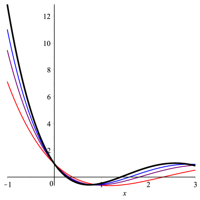
Figure 1: Approximation to Laguerre polynomial, $n=5$

In Figure 2 (left) we show the polynomials in $x^{\mu}$ of degree $n=6$, which coincide at $x=0$ with Hermite polynomial, and which approximate Hermite polynomial at the same time they satisfy a second order fractional differential equation for the values $\mu=0.8$ (in red color), $\mu=0.9$ (purple), $\mu=0.95$ (blue). Classical Hermite polynomial is drawn in black. Figure 2 (right) shows the polynomials of degree $n=6$ associated with classical Hermite polynomials, which satisfy a second order $q$-difference equation for the values $q=0.8$ (in red color), $q=0.9$ (purple), $q=0.95$ (blue). Their value at $x=0$ coincide with that of Hermite polynomial. Classical Hermite polynomial of degree $n=6$ is drawn in black.

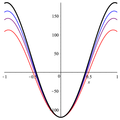
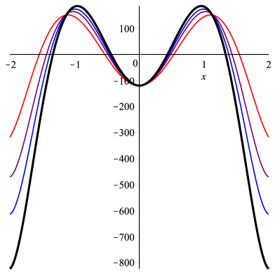
Figure 2: Approximation to Hermite polynomial, $n=6$

Let $\alpha=1$ and $\beta=3/4$. Figure 3 illustrates the approximation made by the polynomials in $x^{\mu}$ of degree $n=6$, which coincide together with their derivative with Jacobi polynomial at $x=0$. We consider the values $\mu=0.8$ (red), $\mu=0.9$ (purple), $\mu=0.95$ (blue) which approach the classical Jacobi polynomial of degree $n=6$, in black. Figure 2 (right) shows the approximation made with polynomials of degree $n=6$ satisfying a second order $q$-difference equation for $q=0.8$ (red), $q=0.9$ (purple), $q=0.95$ (blue), approaching classical Jacobi (black) of degree $n=6$. The polynomials are chosen so that they coincide, together with their first derivative, at $x=0$ with Jacobi polynomial of degree $n=6$.

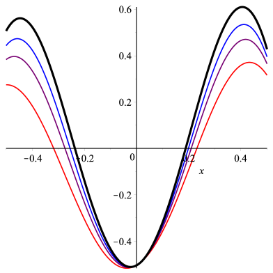
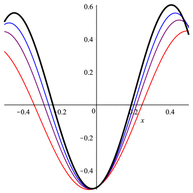
Figure 3: Approximation to Jacobi polynomial, $n=6$

In Figure 4 (left) we display the polynomials in $x^{\mu}$ of degree $n=5$, which coincide at $x=0$ with Bessel polynomial, and which approximate Bessel polynomial and satisfy a second order fractional differential equation for the values $\mu=0.8$ (red), $\mu=0.9$ (purple), $\mu=0.95$ (blue). Classical Bessel polynomial is drawn in black. Figure 4 (right) shows the polynomials of degree $n=5$ associated with classical Bessel polynomials, which satisfy a second order $q$-difference equation for the values $q=0.8$ (in red color), $q=0.9$ (purple), $q=0.95$ (blue). Their value at $x=0$ coincide with that of Bessel polynomial. We observe how they approach the classical Bessel polynomial of degree $n=5$, in black.

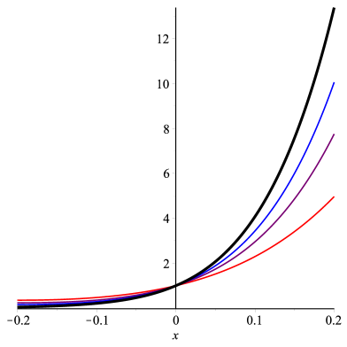
Figure 4: Approximation to Bessel polynomial, $n=5$

The confluence of the zeros of the polynomials can also be stated. As a consequence of the convergence of the coefficients of the generalized polynomials in Section 3 to the coefficients of the classical polynomials, one derives the convergence of their roots. More precisely, for every $n\geq 1$ let $m^{(n)}=(m_{p}^{(n)})_{p\geq 0}$ be a family of sequences of positive real numbers such that $m^{(n)}_{p}\to p!$ when $n\to\infty$, for every $p\geq 0$. Then, for any fixed $N\geq 1$ let $y$ denote the corresponding classical (Laguerre, Hermite, Jacobi or Bessel) polynomial of degree $N$. Then, there exists a sequence $(x_{n})_{n\geq 1}$ of roots of the corresponding generalized polynomial of degree $N$, say $y_{m^{(n)}}$, i.e. $y_{m^{(n)}}(x_{n})=0$ for every $n\geq 1$, such that $x_{n}\to x_{0}$, where $x_{0}$ is a root of $y$. See Proposition 5.2.1 [1], for a proof of the previous statement.

Moreover, the explicit nature of the coefficients of the generalized polynomials constructed in Section 3 allows to give upper bounds on the distance of the roots of the generalized polynomials and the classical ones in virtue of the following classical result.

Theorem 2 (Theorem 1, [4])

Let

$$f(z)=z^{n}+a_{1}z^{n-1}+\ldots+a_{n}=\prod_{i=1}^{n}(z-\alpha_{i}),$$

$$g(z)=z^{n}+b_{1}z^{n-1}+\ldots+b_{n}=\prod_{i=1}^{n}(z-\beta_{i}).$$

Then, there exists a permutation of the roots of $f$ and $g$ such that after such permutation one has

$$\max_{i}|\alpha_{i}-\beta_{i}|\leq 2^{2-1/n}\left(\sum_{k=1}^{n}|a_{k}-b_{k}|\gamma^{n-k}\right)^{1/n},$$

where $\gamma=2\max_{1\leq k\leq n}\left(|a_{k}|^{1/k},|b_{k}|^{1/k}\right)$.

This result refines the previous, not only stating convergence but also a convergence rate of the roots for each of the families of polynomials.

Example 1

We consider the generalized Laguerre polynomials with $\alpha=0$, associated to the sequence $m_{q}=([p]_{q}!)_{p\geq 0}$. Taking into account the coefficients of $y_{L,m_{q}}$ of degree $n$ obtained in Section 4.2, we have that the difference of corresponding roots of $y_{L,m_{q}}$ and the classical Laguerre polynomial of degree $n$ is upper bounded by

$$2^{2-1/n}\left[\sum_{k=1}^{n}\left|\prod_{j=n-k}^{n-1}\frac{[j+1]_{q}([j]_{q}+1)}{[j]_{q}-[n]_{q}}-\frac{n!^{2}}{(n-k)!^{2}(-1)^{k-1}k!}\right|\gamma^{k}\right]^{1/n},$$

with

$$\gamma=2\max_{1\leq k\leq n}\left\{\left(\prod_{j=n-k}^{n-1}\frac{[j+1]_{q}([j]_{q}+1)}{[j]_{q}-[n]_{q}}\right)^{1/k},\left(\frac{n!^{2}}{(n-k)!^{2}(-1)^{k-1}k!}\right)^{1/k}\right\}.$$

5 Conclusions

For each of the families of classical orthogonal polynomials: Laguerre, Hermite, Jacobi and Bessel, we construct for every non-negative integer $n$

1. a second-order moment differential equation,

2. a polynomial of degree $n$,

generalizing the classical equations and polynomials. Two particular manifestations of the sequence of moments, of great importance in applications are considered. In a first application, we are constructing for every $n$ a second-order fractional differential equation and a polynomial-like solution of degree $n$. The adequate modification of the fractional order allows to provide a confluence of the fractional differential equation to the classical second-order differential equation satisfied by the corresponding classical polynomial, whilst the polynomial-like solution tends to the classical polynomial. In a second application, we are constructing for every $n$ a second order $q$-difference equation and a polynomial solution of degree $n$, for every $q>0$. If one considers $q\to 1$, then the $q$-difference equation approaches to the classical second-order differential equation satisfied by the corresponding classical polynomial, and the polynomial solution of the $q$-difference equation tends to the classical orthogonal polynomial.

Many questions are to be answered in a future direction, such as the existence (or not) of a positive measure for which the polynomials obtained are orthogonal. In an affirmative case, is the sequence of moments considered related to the moments of such measure? In this concern, this should be considered as a seminal work to be continued in a future research to answer these and other questions.

References

- [1] M. Artin, Algebra. Englewood Cliffs, NJ: Prentice-Hall. xviii, 1991.
- [2] W. Balser, Formal power series and linear systems of meromorphic ordinary differential equations. Universitext. Springer-Verlag, New York, 2000. xviii+299 pp.
- [3] W. Balser, M. Yoshino, Gevrey order of formal power series solutions of inhomogeneous partial differential equations with constant coefficients. Funkcial. Ekvac. 53 411–434 (2010).
- [4] R. Bhatia, L. Elsner, G. Krause, Bounds for the variation of the roots of a polynomial and the eigenvalues of a matrix. Linear Algebra Appl. 142, 195–209 (1990).
- [5] S. Bochner, Uber Sturm-Liouvillesche Polynomsysteme. Math. Z. 29, 730–736 (1929).
- [6] T. S. Chihara, An Introduction to Orthogonal Polynomials. Mathematics and its Applications Series, Gordon and Breach, New York, 1978.
- [7] M. E. H. Ismail, Classical and Quantum Orthogonal Polynomials in One Variable, Encyclopedia of Mathematics and its Applications, Vol. 98. Cambridge University Press, Cambridge UK, 2005.
- [8] F. H. Jackson, On q-functions and a certain difference operator, Trans. R. Soc. Edinb. 46 (2): 253–281 (1908).
- [9] J. Jiménez-Garrido, S. Kamimoto, A. Lastra, J. Sanz, Multisummability in Carleman ultraholomorphic classes by means of nonzero proximate orders, J. Math. Anal. Appl. 472, No. 1, 627–686 (2019).
- [10] K. H. Kwon, L. L. Littlejohn, Classification of classical orthogonal polynomials. J. Korean Math. Soc. 34, No. 4, 973–1008 (1997).
- [11] A. Lastra, Entire solutions of linear systems of moment differential equations and related asymptotic growth at infinity, Differ. Equ. Dyn. Syst. (2022). https://doi.org/10.1007/s12591-022-00601-2
- [12] A. Lastra, S. Malek, J. Sanz, Summability in general Carleman ultraholomorphic classes, J. Math. Anal. Appl. 430, 1175–1206 (2015).
- [13] A. Lastra, S. Michalik, M. Suwińska, Summability of formal solutions for a family of generalized moment integro-differential equations, Fract. Calc. Appl. Anal. 24, 1445–1476 (2021).
- [14] A. Lastra, S. Michalik, M. Suwińska, Summability of formal solutions for some generalized moment partial differential equations, Result. Math. 76, No. 1, Paper No. 22, 27 p. (2021).
- [15] A. Lastra, S. Michalik, M. Suwińska, Multisummability of formal solutions ofr a family of generalized singularly perturbed moment differential equations, Result. Math. 78, No. 2, Paper No. 49, 31 p. (2023).
- [16] A. Lastra, C. Prisuelos-Arribas, Solutions of linear systems of moment differential equations via generalized matrix exponentials, to appear in J. Differ. Equ. (2023)
- [17] S. Michalik, Analytic solutions of moment partial differential equations with constant coefficients, Funkcial. Ekvac. 56, no. 1, 19–50 (2013).
- [18] S. Michalik, Analytic and summable solutions of inhomogeneous moment partial differential equations, Funkcial. Ekvac. 60, no. 3, 325–351 (2017).
- [19] S. Michalik, B. Tkacz, The Stokes phenomenon for some moment partial differential equations, J. Dyn. Control Syst. 25, no. 4, 573–598 (2019).
- [20] K. B. Oldham, J. Spanier, The fractional calculus. Theory and applications of differentiation and integration to arbitrary order, Mathematics in Science and Engineering. Vol. 111. Academic Press, 1974.
- [21] J. Sanz, Flat functions in Carleman ultraholomorphic classes via proximate orders, J. Math. Anal. Appl. 415(2), 623–643 (2014).
- [22] J. Sanz, Asymptotic analysis and summability of formal power series, Analytic, algebraic and geometric aspects of differential equations, 199–262, Trends Math., Birkhäuser/Springer, Cham, 2017.
- [23] M. Suwińska, Gevrey estimates of formal solutions for certain moment partial differential equations with variable coefficients, J. Dyn. Control Syst. 27, No. 2, 355–370 (2021).
- [24] G. Szegő, Orthogonal Polynomials, Amer. Math. Soc. Coll. Publ, Vol. 23, 4th ed., Amer. Math. Soc., Providence, RI, 1975.