Improving Social Media Popularity Prediction with Multiple Post Dependencies

Abstract.

Social Media Popularity Prediction has drawn a lot of attention because of its profound impact on many different applications, such as recommendation systems and multimedia advertising. Recent work attempts to leverage the content of posts to improve predictive performance. However, few of them consider the multiple dependencies of posts, resulting in their insufficiency to take full advantage of the rich content. To tackle this problem, we propose a novel prediction framework named Dependency-aware Sequence Network (DSN) that exploits both intra- and inter-post dependencies to comprehensively extract content information from posts. For intra-post dependency, DSN adopts a multimodal feature extractor with an efficient fine-tuning strategy to obtain task-specific representations from images and textual information of posts. For inter-post dependency, DSN uses a hierarchical information propagation method to learn category representations that could better describe the difference between posts. DSN also exploits recurrent networks with a series of gating layers for more flexible local temporal processing abilities and multi-head attention for long-term dependencies. The experimental results on the Social Media Popularity Dataset demonstrate the superiority of our method compared to existing state-of-the-art models.

1. Introduction

Social media is an essential part of people’s lives. Understanding the content of social media and forecasting its popularity has drawn a lot of attention from researchers both in academia and industry(Pinto et al., 2013; Khosla et al., 2014; He et al., 2014). Precise popularity prediction can greatly benefit various applications, such as online advertising, content recommendation, and trend analysis. In this paper, we focus on the Social Media Popularity Prediction (SMPP) task, which aims to estimate the target post’s future popularity via plenty of social media data. Typically, the data includes the post content (e.g., images and textual description) and the information of the user who posted it. Among them, user information is usually numerical and easier to process (e.g. number of followers, number of likes), while content information is more complicated and also an important factor for users to interact and share on social media platforms. Engaging content can attract more views, likes, and shares, leading to increased popularity. Conversely, unattractive content is less likely to be engaged with and shared, resulting in less popularity. Therefore, accurately predicting the popularity of a post requires a comprehensive understanding of its content. Conventional SMPP works often manually extract image and textual features, concatenating them directly and then applying machine learning algorithms to make prediction(Wang and Zhang, 2017; He et al., 2019; Kang et al., 2019). This approach does not take full advantage of the post content, resulting in poor predictive performance.

Recently, to make better use of the multimodal content, some works consider the correlation between different modalities within a post, which we called intra-post dependency. Among them, Xu et al. introduce an attention mechanism to assign large weights to more important modalities(Xu et al., 2020). Some others apply multimodal learning methods to align different modalities(Tan et al., 2022; Chen et al., 2022). However, the inter-post dependency, on the other hand, capturing the association between different posts, is not well modeled by their work. For example, posts from the same user or on the same topic may share similar content or attract similar audiences over a sustained period, aggregating information from relevant posts might also enhance the post representation.

In that regard, many researchers adopt sequence modeling to enhance the representation of the target post by incorporating temporally correlated posts. Among them, some extract temporal features of the target user’s posting sequence with sliding window moving average or temporal transformer.(Wang et al., 2020b; Tan et al., 2022), but the methods based on user post sequence ignore the correlation across different users. Wu et al. use the recurrent network and temporal attention mechanisms to model temporal coherence of posts from different users across multiple time-scales(Wu et al., 2017). However, the temporal attention mechanism only considers the release time, other context information is poorly modeled.

Besides the temporal dependency, the categories of posts are also important for modeling the correlation between different posts, which are not well considered by previous works. Posts on social platforms are tagged when they are published to describe the category of the content. These tags are usually hierarchical, for example, photos of the sky could be tagged with landscape, nature, etc to get a higher probability of being viewed. This hierarchy enables category information not only to describe the content of a single post but also to model the correlation between different posts in a fine-grained manner. Figure 1 shows an example of three-level hierarchical category information. The correlation between Garfield and Blue Cat is closer than between it and Corgi, because the former two belong to cats, while the latter belongs to dogs, although they both belong to animals. If we only use the category embedding of a single level, the difference between them could not be accurately modeled.

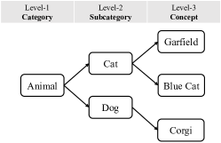
Figure 1. An example of three-level hierarchical category information. From left to right, three levels, i.e., Category, Subcategory, and Concept are presented.

In this paper, we propose a novel deep popularity prediction framework called Dependency-aware Sequence Network (DSN) that leverages both intra- and inter-post dependencies to comprehensively extract content information from posts, which could help us gain a more comprehensive understanding of the factors that contribute to post popularity and improve the accuracy of popularity prediction. We design the architecture to be consistent with multimodal inputs and temporal relationships common to social media popularity prediction - specifically incorporating (1) multimodal feature extractors which explore the correlation between images and textual information of posts. (2) a hierarchical modeling approach that exploits the hierarchical nature of category information to improve post-similarity modeling. (3) a sequence-to-sequence layer with multi-head attention to aggregate post inputs. A series of gating layers are conducted to give the model more flexibility to model the dependencies between posts.

Overall, our contributions can be summarized as follows:

• We fully leverage the importance of the post content for social media popularity prediction by formally defining and modeling intra- and inter-post dependencies.

• We present a novel prediction model called DSN that achieves more precise popularity prediction by jointly modeling the correlation between images and text, the hierarchy of category information, and temporal relevance between posts.

• We conduct extensive experiments to investigate the effectiveness of DSN. The experimental results verify the efficacy and superiority of DSN over state-of-the-art models on Social Media Popularity Dataset. For the convenience of the reproduction of the results, we will make our code publicly available upon publication.

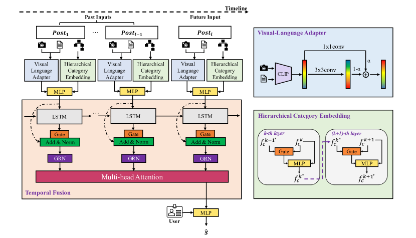
Figure 2. Overview of the proposed model DSN. DSN inputs various content information (i.e. image, text, category) of the post sequence. Visual-Language Adapter (blue region) is used for extracting task-specific multimodal features from images and text. Hierarchical Category Embedding (green region) incorporates the category information across different levels for better describing the difference between posts. Temporal Fusion (orange region) is based on LSTM for local processing and multi-head attention for integrating information at any time step in the post sequence. At last, the enhanced target post feature is fused with user information for the final prediction.

2. Related Work

For the SMPP task, conventional works manually extract image and textual features of posts, fusing them with other metadata (e.g. user information) and make predictions with regression models. (Chen et al., 2019; Ding et al., 2019b). However, these efforts fail to take full advantage of the posts’ rich content information. Recently, many works start to consider the relationship between different modalities, which we denote as intra-post dependency, to enhance the post representation. Among them, Xu et al. propose a multimodal deep learning framework that introduces an attention mechanism to assign large weights to specified modalities(Xu et al., 2020). Chen et al. build two-stream ViLT models for title-visual and tag-visual representations, and design title-tag contrastive learning for two streams to learn the differences between titles and tags(Chen et al., 2022). Tan et al. first perform visual and textual feature extraction respectively and then employ a multimodal transformer ALBEF to align visual and text features in semantic space(Tan et al., 2022). These models only consider the interaction between modalities within a single post, neglecting the correlation between different posts.

To solve this problem, some works target to utilize the temporal correlation between different posts, which is among inter-post dependency, to enhance the feature representation of the post to be predicted. Among them, Wu et al. analyze temporal characteristics of social media popularity, consider the posts as temporal sequence and make a prediction with temporal coherence across multiple time-scales(Wu et al., 2017). Wang et al. use sliding window average to mine potential short-term dependency for each user’s post sequence, then predict by a combined Catboost model to handle the problem of data missing(Wang et al., 2020b). Tan et al. propose a transformer and sliding window average-based timing feature extraction method to reduce the inconsistent distribution between timing features extracted from the training set and test set(Tan et al., 2022). However, these works only concentrate on temporal modeling while ignoring other contextual information. There is not only a temporal relationship between posts, the category difference in post content can also describe the correlation between posts.

In summary, few of existing works jointly model multiple dependencies of posts, leading them to fail to exploit the potential of post content in social media popularity prediction. They either do not consider the relevance of different modalities of the single post or ignore the correlation between posts from different users or other context information (e.g. hierarchical category information). To overcome these problems, our work provides a comprehensive overview of multiple dependencies of posts from both inter- and intra-post perspectives to fully model the content information.

3. PROPOSED METHOD

3.1. Problem Definition

Formally, given a new post $p$ published by user $u$, the problem of predicting its popularity is to estimate how much attention it would receive after its release (e.g. views, clicks or likes etc.). In Social Media Popularity Dataset(Wu et al., 2019) which we use for the experiment, “viewing count” is used to describe the popularity after log-normalization as below:

(1) $$s=\log_{2}\frac{r}{d}+1$$

where $r$ is the viewing count, $d$ is the number of days since the photo was posted and $s$ is the normalized popularity.

In this paper, for any given post $p_{i}$ released at timestamp $t_{i}$, we adopt a chronological sliding window with length $l$ to get the post sequence, which can be defined as $P_{i}=(p_{i-l+1},p_{i-l+2},...,p_{i-1},p_{i})$, where $t_{i-l+1}<t_{i-l+2}<...<t_{i}$. We aim to build a model $F$ which can generate a popularity score $\hat{s_{i}}$ from $P_{i}$ for the post $p_{i}$:

(2) $$\hat{s_{i}}=F(P_{i})$$

3.2. Overview of DSN

We design DSN by using canonical components to efficiently build feature representations for rich contents of posts (i.e. image, text, category) to obtain high predictive performance. The major constituents of DSN are:

1. Visual-Language Adapter to extract visual and textual information, employing a multimodal pre-trained model with an efficient fine-tuning strategy to get task-specific representations.

2. Hierarchical Category Embedding to use a gating mechanism to permit the valuable category information to be passed from coarse to fine granularity. The obtained representation incorporates the information at different levels and can better describe the correlation between posts with different categories.

3. Temporal Fusion to learn both short- and long-term temporal relationships from past posts. A sequence-to-sequence layer is employed for local processing, whereas long-term dependencies are captured using a multi-head attention block. Gating mechanisms are also used to skip over any unused components of the architecture, providing adaptive depth and network complexity.

The overall framework of DSN is shown in Figure 2, with individual components described in detail in the subsequent sections.

3.3. Visual-Language Adapter

Visual-Language Adapter is used to generate a unified representation of visual and textual descriptions of the posts. There has been a lot of vision-language pre-trained models exploring the interaction between these two modalities, one of them is CLIP (Contrastive Language-Image Pretraining)(Radford et al., 2021) which achieves astonishing results on a wide range of vision tasks without any fine-tuning. To close the gap between CLIP and downstream popularity prediction task, inspired by CLIP-Adapter(Gao et al., 2021), we design an efficient feature adapter that only appends a small number of additional learnable layers with residual connections to CLIP’s language and image branches while keeping the original CLIP backbone frozen during fine-tuning.

Specifically, given the input image $I$ and textual description $T$ of the post sequence $P$, the original visual and textual embedding $\mathbf{f}_{v}^{origin},\mathbf{f}_{t}^{origin}\in\mathbb{R}^{l\times d_{origin}}$ are computed with CLIP backbone, where $l$ is the sequence length and $d_{origin}$ is the dimension of the output of the CLIP encoder. After that, two learnable feature adapters $A_{v}(\cdot)$ and $A_{t}(\cdot)$ are adopted to transform $\mathbf{f}_{v}^{origin}$ and $\mathbf{f}_{t}^{origin}$, respectively. In each adapter, we use convolutions with 3x3 filters and ReLU activation function(Glorot et al., 2011) to get adapted features, and convolutions with 1x1 filters to reserve the original knowledge encoded by CLIP. For each convolutional layer, we perform downscaling from $d_{origin}$ to $d_{hidden}$ so that these features could be consistent with other low-dimensional features, eg., the user information of the post). Two trade-off parameters $\alpha$ and $\beta$ are employed as “residual ratio” to help adjust the degree of maintaining the original knowledge for better performance. In summary, for given input $\mathbf{x}$, the feature adapters can be written as:

(3) $$A_{v}(\mathbf{x})=(1-\alpha){{\rm ReLU(Conv}_{3{\rm x}3}(\mathbf{x}))}+\alpha{{\rm Conv}_{1{\rm x}1}(\mathbf{x})}$$

For $A_{t}(x)$, $\alpha$ is replaced with $\beta$. After employing adapters to the original features, we can get new visual and textual feature $\mathbf{f}_{v},\mathbf{f}_{t}\in\mathbb{R}^{l\times d_{hidden}}$:

(4) $$\mathbf{f}_{v} =A_{v}(\mathbf{f}_{v}^{origin})$$

(5) $$\mathbf{f}_{t} =A_{t}(\mathbf{f}_{t}^{origin})$$

3.4. Hierarchical Category Embedding

Hierarchical Category Embedding is to learn category representation which can better describe the correlation between different posts by stacking several HCE layers. Each layer uses a gating mechanism that allows valuable information from the previous layer to pass through and combine with information from this layer to obtain a comprehensive category representation across layers.

Specifically, for the hierarchy category information as shown in figure 1, we denote the original category embedding of level-$k$ learned by the embedding layer as $\mathbf{f}_{c}^{k}\in\mathbb{R}^{l\times h_{hidden}}$. The inputs of the $k$-th HCE layer are the independent category embedding $\mathbf{f}_{c}^{k}$ of level-$k$ and the hierarchical embedding $\mathbf{f}_{c}^{{k-1}^{*}}$ computed by the last layer. The output $\mathbf{f}_{c}^{{k}^{*}}$ of the $k$-th layer would be treated as the input to the next layer for iterative computing:

(6) $$\mathbf{f}_{c}^{k^{*}}={\rm HCE}_{k}\left(\mathbf{f}_{c}^{{k-1}^{*}},\mathbf{f}_{c}^{k}\right)$$

In each HCE layer, we use a gating mechanism based on Gated Linear Unit (GLU)(Dauphin et al., 2017) to compress the information from the previous layer. The more valuable the information of the previous layer is, the more it would be retained. Given input $\mathbf{x},\mathbf{y}\in\mathbb{R}^{l\times d_{hidden}}$, our gating mechanism can be represented as:

(7) $${\rm Gate}_{k}(\mathbf{x},\mathbf{y})=(\mathbf{x}\mathbf{W}_{1,k}+\mathbf{b}_{1,k})\odot\sigma(\mathbf{x}\mathbf{W}_{2,k}+\mathbf{y}\mathbf{W}_{3,k}+\mathbf{b}_{2,k})$$

where $\mathbf{W}_{(.)}\in\mathbb{R}^{d_{hidden}\times d_{hidden}},\mathbf{b}_{(.)}\in\mathbb{R}^{d_{hidden}}$ are the weights and bias, $k$ means the parameters of the gating mechanism are not shared across different HCE layers. $\odot$ is the element-wise Hadamard product, and $\sigma(\cdot)$ is the sigmoid activation function.

With the gating mechanism, we can give the calculation process of the HCE layer in Eq. 6:

(8) $$\mathbf{f}_{c}^{{k-1}^{\prime}} ={\rm Gate}_{k}(\mathbf{f}_{c}^{{k-1}^{*}},\mathbf{f}_{c}^{k})$$

(9) $$\mathbf{f}_{c}^{{k}^{*}} =\left[\mathbf{f}_{c}^{k}\|\mathbf{f}_{c}^{{k-1}^{\prime}}\right]\mathbf{W}_{k}$$

where $\mathbf{W}_{k}\in\mathbb{R}^{2d_{hidden}\times d_{hidden}}$ is the weight of the $k$-th HCE layer and $\|$ is the concatenation operation. Eq. 8 generates a gating of cross-layer information through a sigmoid function to control the inflow of relevant information from the previous layers. A linear transformation is used in Eq. 9 to combine the useful information from previous layers with the independent information of the current layer.

We stack three HCE layers to model the 3-level hierarchy category information given by the dataset. The output $\mathbf{f}_{c}^{{3}^{*}}$ of the last HCE layer incorporates category information across different levels and can express the differences between posts in a more fine-grained manner. We denote $\mathbf{f}_{c}^{{3}^{*}}$ as $\mathbf{f}_{c}$ for a unified description. Then $\mathbf{f}_{c}$ is concatenated with visual-language features computed by Visual-Language Adapter as the post representations $\mathbf{f}\in\mathbb{R}^{l\times 3d_{hidden}}$ of the post sequence:

(10) $$\mathbf{f}=\left[\mathbf{f}_{v}||\mathbf{f}_{t}||\mathbf{f}_{c}\right]$$

3.5. Temporal Fusion

Temporal Fusion is to learn temporal dependency between posts. Note that $P_{l}$ might contains posts from several different users, which presents a challenge for the temporal modeling of post sequences. We construct the module based on LSTM which is commonly used for local processing. Inspired by Temporal Fusion Transformer(Lim et al., 2021), we use the gating mechanism and residual connection to control the fusion of the temporal information learned by LSTM and the original features. Specifically, given the input $\mathbf{f}\in\mathbb{R}^{l\times 3d_{hidden}}$, the output $\mathbf{\Phi}\in\mathbb{R}^{l\times d_{hidden}}$ of local temporal processing can be calculated as follow:

(11) $$\mathbf{O} ={\rm LSTM}(\mathbf{f})$$

(12) $$\mathbf{\Theta} ={\rm LayerNorm(Gate}_{o}(\mathbf{O})+\mathbf{f}\mathbf{W})$$

(13) $$\mathbf{\Phi} ={\rm GRN}_{\theta}(\mathbf{\Theta})$$

where LayerNorm is standard layer normalization of (Ba et al., 2016), and $\mathbf{W}\in\mathbb{R}^{3d_{hidden}\times d_{hidden}}$ is the linear transformation for downscaling. The gating mechanism is a version of Eq.7 with only one input. $o$ denotes the parameters of the gating mechanism here are shared across the entire layer. The Gated Residual Network (GRN)(Lim et al., 2021) in Eq.13 could provide adaptive depth to the model. Given an input $\mathbf{x}$, the GRN yields:

(14) $${\rm GRN}_{\theta}(\mathbf{x}) ={\rm LayerNorm}(\mathbf{x}+{\rm Gate_{\theta}(\mathbf{\eta}_{1})})$$

(15) $$\mathbf{\eta}_{1} =\mathbf{W}_{1,\theta}\mathbf{\eta}_{2}+\mathbf{b}_{1,\theta}$$

(16) $$\mathbf{\eta}_{2} ={\rm ELU}(\mathbf{W}_{2,\theta}\mathbf{x}+\mathbf{b}_{2,\theta})$$

where ELU is the Exponential Linear Unit activation function(Clevert et al., 2015). The gating mechanism and residual structure in GRN could provide flexibility to apply non-linear processing when needed. If necessary, the layer could be entirely skipped, as the outputs of Gate may all be close to zero to suppress nonlinear contributions.

We further adopt multi-head attention(Vaswani et al., 2017) to learn long-term dependency in the post sequence. Here, the attention mechanism computes dot-product attention, which is defined as:

(17) $${\rm Attetion}(\mathbf{Q,K,V})={\rm Softmax}(\mathbf{Q}\mathbf{K}^{T}/\sqrt{d_{hidden}})\mathbf{V}$$

where $\mathbf{Q}$ denotes the ’query’, $\mathbf{K}$ the ’key’ and $\mathbf{V}$ the ’value’. While the usual sequence-sequence model calculates the attention between any two positions, our model DSN is concerned with the correlation between the target post and other posts in the sequence. Given the input $\mathbf{\Phi}$ yields by Eq.13, the ’query’, ’key’ and ’value could be obtained as below:

(18) $$\mathbf{q}=\mathbf{\Phi}_{l}\mathbf{W}^{Q},\mathbf{K}=\mathbf{\Phi}_{1:l-1}\mathbf{W}^{K},\mathbf{V}=\mathbf{\Phi}_{1:l-1}\mathbf{W}^{V}$$

where $\mathbf{W}^{Q},\mathbf{W}^{K},\mathbf{W}^{V}\in\mathbb{R}^{d_{hidden}\times d_{hidden}}$ are the weight matrices. $\mathbf{\Phi}_{l}\in\mathbb{R}^{d_{hidden}}$ is the feature of the target post and $\mathbf{\Phi}_{1:l-1}\in\mathbb{R}^{(l-1)\times d_{hidden}}$ are of other posts. We then use the above dot-product attention to get the hidden representations of the neighbor posts $\mathbf{h}\in\mathbb{R}^{d_{hidden}}$:

(19) $$\mathbf{h}={\rm Attetion(}\mathbf{q},\mathbf{K},\mathbf{V})\\$$

To combine neighbor post representations $\mathbf{h}$ with the target post feature $\mathbf{\Phi}_{l}$, we concatenate them and feed them into a feed-forward neural network to capture non-linear interactions between the features as in (Vaswani et al., 2017):

(20) $$\mathbf{\tilde{h}}={\rm FFN}\left(\mathbf{h}||\mathbf{\Phi}_{l}\right)=\rm{ReLU}(\left[\mathbf{h}||\mathbf{\Phi}_{\textit{l}}\right]\mathbf{W}_{1}+\mathbf{b}_{1})\mathbf{W}_{2}+\mathbf{b}_{2}$$

where $\mathbf{W}_{1}\in\mathbb{R}^{2d_{hidden}\times d_{hidden}}$, $\mathbf{W}_{2}\in\mathbb{R}^{d_{hidden}\times d_{hidden}},\mathbf{b}_{1},\mathbf{b}_{2}\in\mathbb{R}^{d_{hidden}}$, and $\mathbf{\tilde{h}}\in\mathbb{R}^{d_{hidden}}$ is the final output representing the target post feature.

3.6. Prediction Module

Considering the importance of user information shown in previous works, we choose some metadata from the official Social Media Popularity Dataset. We also follow the HyFea(Lai et al., 2020) method to obtain more numerical information from users’ websites. All the user information we use is listed in Table 1. For categorical data Uid, we adopt a learnable embedding layer to transform it into numerical features. For PublishTime, we convert the timestamp to month, day and hour and process them by one-hot encoding. The rest of the data are all numerical and we scale them by z-score normalization. All information about the user who posted the target post $p$ is concatenated as user features $\mathbf{u}$. After concatenating user features $\mathbf{u}$ and post features $\mathbf{\tilde{h}}$, a two-layer MLP (Multi-Layer Perception) is adopted to learn the relationship between the user and post and perform the popularity prediction:

(21) $$\hat{s}={\rm MLP}(\left[\mathbf{\tilde{h}}||\mathbf{u}\right])$$

Finally, we minimize the MSE (Mean Square Error) loss to optimize the predicted popularity value $\hat{s}$.

Data Entry	Description
Uid	The user this post belongs to.
Ispublic	Is the post authenticated with ’read’ permissions.
Ispro	Is the user belong to pro member.
Latitude	The latitude of the posting location.
Longitude	The longitude of the posting location.
GeoAccuracy	The accuracy level of the location information.
Postdate	The publish timestamp of the post.
$\rm{Followers^{*}}$	The number of people the user follows.
$\rm{Following^{*}}$	The number of followers of the user.
$\rm{Views^{*}}$	The number of views of the user’s posts.
$\rm{Tags^{*}}$	The number of tags of the user’s posts.
$\rm{Faves^{*}}$	The number of faves of the user’s posts.
$\rm{InGroups^{*}}$	The number of groups the user belongs to.

Table 1. The user information used for prediction. The data entries with $*$ are crawled from the users’ homepages according to Hyfea’s method(Lai et al., 2020), and others are from the official SMPD(Wu et al., 2019).

4. Experiment

4.1. Dataset

We use the Social Media Prediction Dataset (SMPD)(Wu et al., 2019) collected from Flickr, which is widely used by previous works(Ding et al., 2019b; Xu et al., 2020; Kang et al., 2019; Tan et al., 2022; Chen et al., 2022), to evaluate the performance of our method. SMPD contains 486k posts from 69k users. For each post, both visual and textual information are provided along with multiple metadata and category information. The category information is depicted in a 3-level manner. The number of categories in the three levels is 11, 77, and 668, respectively. These posts are sorted by posting time, split for train and test by ratio 2:1. The labeled training set is released to participants, and the labels of the test set for final evaluation have not been released. We use the labeled training set to evaluate our algorithm. We split the data chronologically based on the time order of posts. The ratio of the split is 8:1:1, meaning that 80% of the data is used for training, 10% for validation, and 10% for testing.

4.2. Implementation Details

We use CLIP(Radford et al., 2021) as the backbone of Visual-Language Adapter. The dimensions of all hidden layers in the model are set to 256. The number of attention heads is set to 4. The length of the inputted post sequence is set to 16. We optimize the model by Adam optimizer(Kingma and Ba, 2014) with the learning rating of 1e-3 and weight decay of 1e-4 for 10 epochs. The batch size is 512. To avoid over-fitting, we set dropout to 0.25. The experiments are implemented with PyTorch and conducted on a single NVIDIA GTX 1080 GPU.

4.3. Evaluation Metrics

To evaluate the prediction performance, we use a precision metric Mean Absolute Error (MAE) and a correlation metric Spearman Ranking Correlation (SRC) as in (Wu et al., 2017). If there are k samples, given ground-truth popularity set $S$ and predicted popularity set $\hat{S}$ varying from 0 to 1, the MAE can be expressed as:

(22) $$MAE=\frac{1}{k}\sum_{i=1}^{n}\left|\hat{S}_{i}-S_{i}\right|$$

the SRC is used to measure the ranking correlation between $\hat{S}$ and $S$:

(23) $$SRC=\frac{1}{k-1}\sum_{i=1}^{k}\left(\frac{S_{i}-\bar{S}}{\sigma_{S}}\right)\left(\frac{\hat{S}_{i}-\overline{\hat{S}}}{\sigma_{\hat{S}}}\right)$$

Lower MAE / higher SRC refers to better performance.

4.4. Baselines

To showcase the effectiveness of the proposed model, we compare its prediction performance with six state-of-the-art baseline models of SMPP. We summarize dependencies used by different models in Table 2 for comparison.

Baseline 1: Deep Context Neural Network (DTCN)(Wu et al., 2017). Wu et al. use ResNet(He et al., 2016) to generate visual representation, jointly embedding them with user feature into in a common space. Based on the embedded sequence over time, they adopt LSTM(Hochreiter and Schmidhuber, 1997) and temporal attention to predict popularity with temporal coherence across multiple time scales.

Baseline 2: Multiple Layer Perceptron (MLP)(Ding et al., 2019b). Ding et al. use ResNet(He et al., 2016), NIMA(Talebi and Milanfar, 2018) and IIPA(Ding et al., 2019a) to generate deep visual representations, aesthetics scores, and intrinsic popularity scores, respectively. They adopt BERT(Devlin et al., 2018) to get text feature and feed them together with user feature into MLP to make prediction.

Baseline 3: MLP with Attention Mechanism (Att-MLP)(Xu et al., 2020). Xu et al. adopt ResNet(He et al., 2016) and Word2Vec(Mikolov et al., 2013) for visual and text respectively. They consider specific modalities are of greater importance on the popularity of the post, using an attention mechanism to control how much attention should be attended to each modality.

Baseline 4: Feature Generalization Framework with Combined Catboost (Catboost)(Kang et al., 2019). Kang et al. adopt ResNet(He et al., 2016) for visual features. They use BERT(Devlin et al., 2018), FastText(Joulin et al., 2016), TFIDF, and LDA(Blei et al., 2003) to get text features. They do sliding window moving average over temporal ordered features to model dependency for each user’s posts.

Baseline 5: Efficient Multi-View multimodal Data Processing Framework (Multi-view)(Tan et al., 2022). Tan et al. use ALBEF(Li et al., 2021) which consists of an image encoder, a text encoder, and a multimodal encoder to extract visual-language representation features. They also use sliding window moving average and transformer based-methods, including Performer(Choromanski et al., 2020) and Linformer(Wang et al., 2020a) to extract temporal features for each user’s posts.

Baseline 6: Title-and-Tag Contrastive Vision-and-Language Transformer (TTC-VLT)(Chen et al., 2022). Chen et al. use pre-trained ViLT(Kim et al., 2021) to extract both image and text features. To tackle the problems caused by the difference between titles and tags, they build 2 two-stream ViLT models for title-visual and tag-visual, exploiting contrastive learning to estimate a lower bound of the mutual information between titles and tags.

Methods	Dependencies		MAE$\downarrow$	SRC$\uparrow$
	intra-post	inter-post
DTCN(Wu et al., 2017)	$/$	$\mathrm{T}$	1.532	0.624
MLP(Ding et al., 2019b)	$/$	$/$	1.483	0.631
Attention MLP(Xu et al., 2020)	$\mathrm{V}$-$\mathrm{L}$	$/$	1.453	0.635
Catboost(Kang et al., 2019)	$/$	$\mathrm{T}$	1.442	0.663
Multi-view(Tan et al., 2022)	$\mathrm{V}$-$\mathrm{L}$	$\mathrm{T}$	1.387	0.693
TTC-VLT(Chen et al., 2022)	$\mathrm{V}$-$\mathrm{L}$	$/$	1.346	0.711
DSN (Ours)	$\mathrm{V}$-$\mathrm{L}$	$\mathrm{T}$ & $\mathrm{C}$	$\mathbf{1.192^{*}}$	$\mathbf{0.763^{*}}$

Table 2. Overall comparison results with state-of-the-art methods on SMPD dataset. Lower MAE / higher SRC refers to better performance. The post dependencies utilized by the methods are listed by intra- and inter-post. V-L denotes visual-language, T denotes temporal and C denotes category. A paired t-test is performed and $*$ indicates a statistical significance $p<0.001$ compared to the best baseline method. The best results are in bold.

4.5. Overall Performance

We report the best prediction results of our proposed method and the compared models in Table 2. Overall, our model achieves the best prediction performance with the minimal MAE of 1.192 and the highest SRC of 0.763. Compared with the strongest baseline model, i.e. TTC-VLT(Chen et al., 2022), our method reduces MAE by 11.0% and improves SRC by 7.3%.

From the perspective of the dependencies, Attention MLP(Xu et al., 2020) and Catboost(Kang et al., 2019) utilize intra-post and inter-post dependencies, respectively, making them superior to MLP(Ding et al., 2019b). However, the quality of features is also important, e.g., although DTCN(Wu et al., 2017) exploits the temporal dependency between posts, it extracts insufficient visual features and does not utilize textual features, which leads to unsatisfied performance. Multi-view(Tan et al., 2022) both consider intra- and inter-post dependencies, making them more effective than the above baselines. TTC-VLT(Chen et al., 2022) considers the relevance of image and different types of textual information, i.e. titles and tags, which makes up for the fact that it does not exploit the inter-post dependency.

Overall, besides image-text dependency and temporal dependency, our method further considers the hierarchical nature of categories, allowing for more fine-grained modeling of inter-post dependency. Jointly learning both intra- and inter-post dependency makes our model achieve the best prediction result.

$l$	1	4	8	16	32	64
MAE$\downarrow$	1.245	1.221	1.192	1.198	1.217	1.232
SRC$\uparrow$	0.743	0.759	0.763	0.763	0.758	0.747

Table 3. Influence of sequence length. $l=8$ is the length used by DSN. The best results are in bold.

User	Image	Text	Category	MAE$\downarrow$	SRC$\uparrow$
✓	✗	✗	✗	1.350	0.681
✓	✓	✗	✗	1.304	0.717
✓	✗	✓	✗	1.303	0.707
✓	✗	✗	✓	1.269	0.727
✓	✓	✓	✗	1.289	0.723
✓	✓	✗	✓	1.215	0.752
✓	✗	✓	✓	1.231	0.741
✓	✓	✓	✓	1.192	0.763

Table 4. Ablations on different combinations of features. The last line is the features used by DSN. The best results are in bold.

4.6. Ablation Study

To further illustrate the advantages of the proposed model, we also conduct ablation studies to evaluate the contribution of each module.

4.6.1. Ablating the sequence length $l$

We experiment on sequence length $l$ to find how much past inputs are best for predicting the target post. From Table 3, we can see the result is worst when $l=1$, because the model makes predictions only by the information of the target post, ignoring the inter-post dependency. As the sequence length gets longer, the best results are obtained at $l=8$. The results at $l=16$ are close to optimal. Then as $l$ continues to increase, the results start to get worse. The post sequence of appropriate length facilitates the model to learn inter-post dependency, which improves the prediction performance compared to using only the feature of the target post itself. However, the too-long sequence may incorporate irrelevant information, making it difficult for the model to capture the correct correlation, thus compromising the prediction results.

4.6.2. Contributions of Different Features

In order to better understand the contribution of multimodal content (image, text and category features) to the prediction performance, we take user information as the basic feature and add different combinations of the other three features to evaluate the model performance. Table 4 shows the results of the ablation study, from which we find that each feature improves the result to a certain extent, and more features produce better prediction performance. In terms of the effect of different features, the category information improves the results more than images and text. The reason might be that compared with the abstract semantics contained in text and images, category information can more accurately represent whether a post belongs to the popular type. The text data improves the performance least, and the reason might be that the text data in SMPD contains a large amount of semantically ambiguous expressions (e.g. meaningless sequence of numbers or abbreviation of words), which could make it difficult for the model to learn useful textual information.

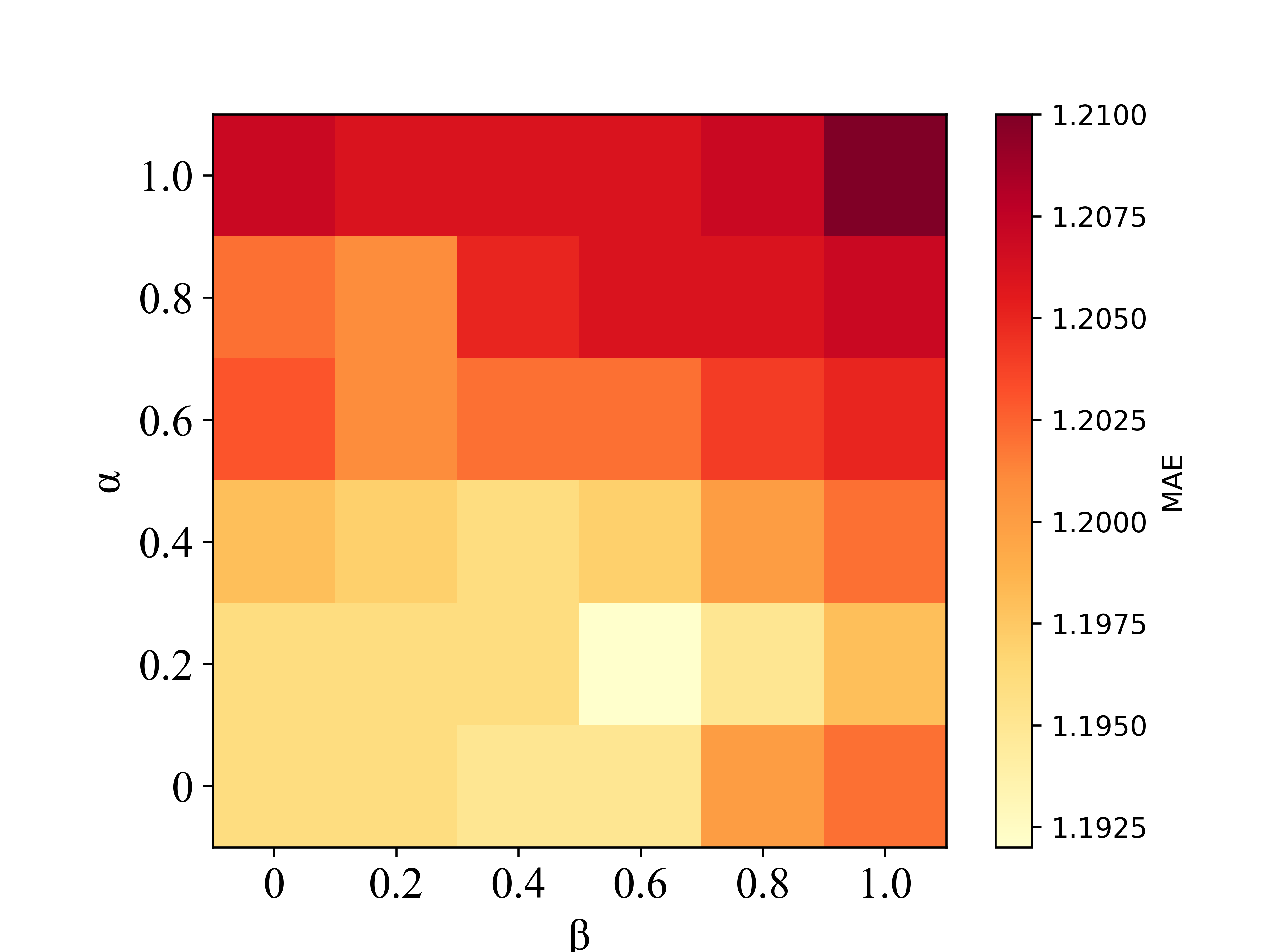
Figure 3. Comparison of MAE (Mean Absolute Error) for different values of residual ratios $\alpha$ (visual) and $\beta$ (textual) in Visual-Language Adapter of DSN. The lighter color of the heat map means lower MAE, i.e. better results. The best result that MAE $=1.192$ is achieved when $\alpha=0.2$ and $\beta=0.6$.

4.6.3. Ablating the encoders of Visual-Language Adapter

We further verify the effectiveness of using multimodal encoders to extract image and textual features. We choose the state-of-the-art encoders Swintransformer(Liu et al., 2021) and BERT(Devlin et al., 2018) for images and text, respectively, to compare with CLIP used in DSN. To fairly compare the performance of different encoders, we set the residual ratios $\alpha$ and $\beta$ to $1$, i.e., no fine-tuning is adopted. We will verify the effectiveness of our fine-tuning strategy later. Table 5 shows the prediction results for different combinations of image and text encoders. We can find that replacing the unimodal encoders with the text or image branch of CLIP, respectively, has some improvement on the results. And encoding both images and text with CLIP achieves significantly better results than using BERT and SwinTransformer. This means that learning the dependency between images and text with a multimodal encoder like CLIP is useful for improving prediction performance.

Methods	MAE$\downarrow$	SRC$\uparrow$
SwinTransformer + BERT	1.269	0.723
SwinTransformer + CLIP-Text	1.246	0.731
CLIP-Image + BERT	1.237	0.746
CLIP-Image + CLIP-Text	1.210	0.755

Table 5. Comparison with different combinations of image and text encoders. The last line is the encoders used by DSN. The best results are in bold.

Methods	MAE$\downarrow$	SRC$\uparrow$
First level	1.281	0.724
Second level	1.269	0.733
Third level	1.253	0.747
Concatenation of three levels	1.249	0.752
Summation of three levels	1.238	0.751
HCE	1.192	0.763

Table 6. Comparison with different methods to encode three-level category information. HCE denotes the Hierarchical Category Embedding used by DSN. The best results are in bold.

Methods	MAE$\downarrow$	SRC$\uparrow$
DSN (w/o short-term dependency)	1.223	0.754
DSN (w/o long-term dependency)	1.237	0.749
DSN	1.192	0.763

Table 7. Ablations on Temporal Fusion of DSN. The long-term dependency denotes the attention mechanism and the short-term dependency is LSTM with the gating layers. The best results are in bold.

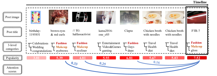
Figure 4. Qualitative results of our DSN when the sequence length $l=8$. The target predicted post is marked on the far right by the solid box. The ground-truth popularity value is $7.52$ and the prediction result is $7.36$. We show the image, title and category information of each post in the sequence. The ground-truth popularity values and attention scores are also presented, which reflects that posts with similar content share similar popularity. Therefore DSN is able to improve the prediction performance of the target post by aggregating the information of related posts.

4.6.4. Ablating the residual ratios of Visual-Language Adapter

To understand the effectiveness of our fine-tuning strategy in Visual-Language Adapter, we perform an ablation study on the residual ratios $\alpha$ and $\beta$ of visual and textual features. Both ratios take values in the range $\left[0,1\right]$, and in the experiment, discrete sampling is performed in steps of 0.2. Note that the residual ratios control how much knowledge would be reserved from the pre-trained CLIP model. So when the ratio equals 1, there is no new knowledge is learned, and when the ratio is set to 0, the feature would be fully adapted. Figure 3 shows the prediction results for different combinations of two ratios. Note that a darker color means a higher MAE, i.e., a worse result. Generally, We can see that when the ratio increases, the MAE also increases at the same time, which means that adjusting the representation as much as possible can produce better results. However, there is an obvious drop in MAE when $\alpha$ increases from 0 to 0.2, which means retaining some of the original knowledge still helps to improve the prediction results. The best result that MAE $=1.192$ is achieved when $\alpha=0.2$ and $\beta=0.6$, respectively, which means compared with text, image features need more fine-tuning to adapt to our task.

4.6.5. Effectiveness of Hierarchical Category Embedding

We also perform an ablation study on Hierarchical Category Embedding to demonstrate the effectiveness of incorporating the category information. We experiment with different methods to obtain category features, including using category embedding of a single level, directly concatenating three levels together, and the HCE method we proposed in DSN, respectively. From Table 6, compared with only using the category information of one level or simple fusion method (i.e., summation and concatenation), DSN further considers the hierarchical nature of different levels, compressing coarse-grained category information as much as possible while keeping fine-grained category information, which could better model the dependency between different posts and achieve more promising results.

4.6.6. Effectiveness of Temporal Fusion

We also verify the effectiveness of Temporal Fusion, which aims to model both local and long-term dependencies. The temporal fusion has two main components, LSTM with gating layers for local processing and multi-head attention for long-term dependency. We remove each of these two components separately to evaluate the effectiveness of different dependencies. Table 7 shows that removing different components caused different degrees of degradation in prediction performance. When we remove the local processing component, the attention mechanism treats posts as an unordered sequence and the short-term temporal dependency between posts would be lost, so the results get worse. Then we keep the local processing but remove the attention, the model cannot handle long-term dependencies, also leading to worse results.

4.7. Qualitative Results

We present a prediction example in the test dataset when the sequence length $l=8$ in Figure 4. The target post is on the right highlighted by a solid box. We show the image, title and category information of each post in the sequence. The ground-truth popularity value of the target post is $7.36$ and the prediction result is $7.52$. Note that the popularity values of other posts are used for visualization purposes only and are not used to predict the target posts. We can see the title is a simple description of the content of the image, so mining the correlation of images and text can help DSN better model the content of the post. The categories of the target post are fashion-makeup-gloss. The popularity values and attention scores show that posts with similar content (i.e., images, text and categories) share similar popularity, so DSN could improve prediction performance by integrating posts that have similar content.

5. Conclusion

In this work, we present Dependency-aware Sequence Network (DSN), a novel prediction framework for social media popularity prediction. Based on the ability of post content to provide valuable clues for popularity prediction, we jointly model multiple post dependencies for better post representations, leading to significantly better performance compared to competitive baselines on Social Media Popularity Dataset. Extensive ablation studies also show that our proposed (i) visual-language adapter (ii) hierarchical category embedding (iii) adaptive temporal fusion method provide significant contributions to our model’s performance. In the future, we plan to consider the dependency between users (e.g. social network graph or information cascade graph) to further improve social media popularity prediction.

References

- (1)
- Ba et al. (2016) Jimmy Lei Ba, Jamie Ryan Kiros, and Geoffrey E Hinton. 2016. Layer normalization. arXiv preprint arXiv:1607.06450 (2016).
- Blei et al. (2003) David M Blei, Andrew Y Ng, and Michael I Jordan. 2003. Latent dirichlet allocation. Journal of machine Learning research 3, Jan (2003), 993–1022.
- Chen et al. (2019) Junhong Chen, Dayong Liang, Zhanmo Zhu, Xiaojing Zhou, Zihan Ye, and Xiuyun Mo. 2019. Social media popularity prediction based on visual-textual features with xgboost. In Proceedings of the 27th ACM International Conference on Multimedia. 2692–2696.
- Chen et al. (2022) Weilong Chen, Chenghao Huang, Weimin Yuan, Xiaolu Chen, Wenhao Hu, Xinran Zhang, and Yanru Zhang. 2022. Title-and-Tag Contrastive Vision-and-Language Transformer for Social Media Popularity Prediction. In Proceedings of the 30th ACM International Conference on Multimedia. 7008–7012.
- Choromanski et al. (2020) Krzysztof Choromanski, Valerii Likhosherstov, David Dohan, Xingyou Song, Andreea Gane, Tamas Sarlos, Peter Hawkins, Jared Davis, Afroz Mohiuddin, Lukasz Kaiser, et al. 2020. Rethinking attention with performers. arXiv preprint arXiv:2009.14794 (2020).
- Clevert et al. (2015) Djork-Arné Clevert, Thomas Unterthiner, and Sepp Hochreiter. 2015. Fast and accurate deep network learning by exponential linear units (elus). arXiv preprint arXiv:1511.07289 (2015).
- Dauphin et al. (2017) Yann N Dauphin, Angela Fan, Michael Auli, and David Grangier. 2017. Language modeling with gated convolutional networks. In International conference on machine learning. PMLR, 933–941.
- Devlin et al. (2018) Jacob Devlin, Ming-Wei Chang, Kenton Lee, and Kristina Toutanova. 2018. Bert: Pre-training of deep bidirectional transformers for language understanding. arXiv preprint arXiv:1810.04805 (2018).
- Ding et al. (2019a) Keyan Ding, Kede Ma, and Shiqi Wang. 2019a. Intrinsic image popularity assessment. In Proceedings of the 27th ACM International Conference on Multimedia. 1979–1987.
- Ding et al. (2019b) Keyan Ding, Ronggang Wang, and Shiqi Wang. 2019b. Social media popularity prediction: A multiple feature fusion approach with deep neural networks. In Proceedings of the 27th ACM International Conference on Multimedia. 2682–2686.
- Gao et al. (2021) Peng Gao, Shijie Geng, Renrui Zhang, Teli Ma, Rongyao Fang, Yongfeng Zhang, Hongsheng Li, and Yu Qiao. 2021. Clip-adapter: Better vision-language models with feature adapters. arXiv preprint arXiv:2110.04544 (2021).
- Glorot et al. (2011) Xavier Glorot, Antoine Bordes, and Yoshua Bengio. 2011. Deep sparse rectifier neural networks. In Proceedings of the fourteenth international conference on artificial intelligence and statistics. JMLR Workshop and Conference Proceedings, 315–323.
- He et al. (2016) Kaiming He, Xiangyu Zhang, Shaoqing Ren, and Jian Sun. 2016. Deep residual learning for image recognition. In Proceedings of the IEEE conference on computer vision and pattern recognition. 770–778.
- He et al. (2014) Xiangnan He, Ming Gao, Min-Yen Kan, Yiqun Liu, and Kazunari Sugiyama. 2014. Predicting the popularity of web 2.0 items based on user comments. In Proceedings of the 37th international ACM SIGIR conference on Research & development in information retrieval. 233–242.
- He et al. (2019) Ziliang He, Zijian He, Jiahong Wu, and Zhenguo Yang. 2019. Feature Construction for Posts and Users Combined with LightGBM for Social Media Popularity Prediction. In ACM Multimedia. ACM, 2672–2676.
- Hochreiter and Schmidhuber (1997) Sepp Hochreiter and Jürgen Schmidhuber. 1997. Long short-term memory. Neural computation 9, 8 (1997), 1735–1780.
- Joulin et al. (2016) Armand Joulin, Edouard Grave, Piotr Bojanowski, and Tomas Mikolov. 2016. Bag of tricks for efficient text classification. arXiv preprint arXiv:1607.01759 (2016).
- Kang et al. (2019) Peipei Kang, Zehang Lin, Shaohua Teng, Guipeng Zhang, Lingni Guo, and Wei Zhang. 2019. Catboost-based Framework with Additional User Information for Social Media Popularity Prediction. In ACM Multimedia. ACM, 2677–2681.
- Khosla et al. (2014) Aditya Khosla, Atish Das Sarma, and Raffay Hamid. 2014. What makes an image popular?. In Proceedings of the 23rd international conference on World wide web. 867–876.
- Kim et al. (2021) Wonjae Kim, Bokyung Son, and Ildoo Kim. 2021. Vilt: Vision-and-language transformer without convolution or region supervision. In International Conference on Machine Learning. PMLR, 5583–5594.
- Kingma and Ba (2014) Diederik P. Kingma and Jimmy Ba. 2014. Adam: A Method for Stochastic Optimization. CoRR abs/1412.6980 (2014).
- Lai et al. (2020) Xin Lai, Yihong Zhang, and Wei Zhang. 2020. HyFea: Winning Solution to Social Media Popularity Prediction for Multimedia Grand Challenge 2020. In Proceedings of the 28th ACM International Conference on Multimedia. 4565–4569.
- Li et al. (2021) Junnan Li, Ramprasaath Selvaraju, Akhilesh Gotmare, Shafiq Joty, Caiming Xiong, and Steven Chu Hong Hoi. 2021. Align before fuse: Vision and language representation learning with momentum distillation. Advances in neural information processing systems 34 (2021), 9694–9705.
- Lim et al. (2021) Bryan Lim, Sercan Ö Arık, Nicolas Loeff, and Tomas Pfister. 2021. Temporal fusion transformers for interpretable multi-horizon time series forecasting. International Journal of Forecasting 37, 4 (2021), 1748–1764.
- Liu et al. (2021) Ze Liu, Yutong Lin, Yue Cao, Han Hu, Yixuan Wei, Zheng Zhang, Stephen Lin, and Baining Guo. 2021. Swin Transformer: Hierarchical Vision Transformer using Shifted Windows. In ICCV. IEEE, 9992–10002.
- Mikolov et al. (2013) Tomas Mikolov, Kai Chen, Greg Corrado, and Jeffrey Dean. 2013. Efficient estimation of word representations in vector space. arXiv preprint arXiv:1301.3781 (2013).
- Pinto et al. (2013) Henrique Pinto, Jussara M Almeida, and Marcos A Gonçalves. 2013. Using early view patterns to predict the popularity of youtube videos. In Proceedings of the sixth ACM international conference on Web search and data mining. 365–374.
- Radford et al. (2021) Alec Radford, Jong Wook Kim, Chris Hallacy, Aditya Ramesh, Gabriel Goh, Sandhini Agarwal, Girish Sastry, Amanda Askell, Pamela Mishkin, Jack Clark, et al. 2021. Learning transferable visual models from natural language supervision. In International Conference on Machine Learning. PMLR, 8748–8763.
- Talebi and Milanfar (2018) Hossein Talebi and Peyman Milanfar. 2018. NIMA: Neural image assessment. IEEE transactions on image processing 27, 8 (2018), 3998–4011.
- Tan et al. (2022) YunPeng Tan, Fangyu Liu, BoWei Li, Zheng Zhang, and Bo Zhang. 2022. An Efficient Multi-View Multimodal Data Processing Framework for Social Media Popularity Prediction. In Proceedings of the 30th ACM International Conference on Multimedia. 7200–7204.
- Vaswani et al. (2017) Ashish Vaswani, Noam Shazeer, Niki Parmar, Jakob Uszkoreit, Llion Jones, Aidan N Gomez, Łukasz Kaiser, and Illia Polosukhin. 2017. Attention is all you need. Advances in neural information processing systems 30 (2017).
- Wang et al. (2020b) Kai Wang, Penghui Wang, Xin Chen, Qiushi Huang, Zhendong Mao, and Yongdong Zhang. 2020b. A Feature Generalization Framework for Social Media Popularity Prediction. In Proceedings of the 28th ACM International Conference on Multimedia. 4570–4574.
- Wang et al. (2020a) Sinong Wang, Belinda Z Li, Madian Khabsa, Han Fang, and Hao Ma. 2020a. Linformer: Self-attention with linear complexity. arXiv preprint arXiv:2006.04768 (2020).
- Wang and Zhang (2017) Wen Wang and Wei Zhang. 2017. Combining Multiple Features for Image Popularity Prediction in Social Media. In ACM Multimedia. ACM, 1901–1905.
- Wu et al. (2017) Bo Wu, Wen-Huang Cheng, Yongdong Zhang, Qiushi Huang, Jintao Li, and Tao Mei. 2017. Sequential Prediction of Social Media Popularity with Deep Temporal Context Networks. In Proceedings of the Twenty-Sixth International Joint Conference on Artificial Intelligence, IJCAI 2017, Melbourne, Australia, August 19-25, 2017. ijcai.org, 3062–3068.
- Wu et al. (2019) Bo Wu, Wen-Huang Cheng, Peiye Liu, Bei Liu, Zhaoyang Zeng, and Jiebo Luo. 2019. SMP challenge: An overview of social media prediction challenge 2019. In Proceedings of the 27th ACM International Conference on Multimedia. 2667–2671.
- Xu et al. (2020) Kele Xu, Zhimin Lin, Jianqiao Zhao, Peicang Shi, Wei Deng, and Huaimin Wang. 2020. Multimodal deep learning for social media popularity prediction with attention mechanism. In Proceedings of the 28th ACM International Conference on Multimedia. 4580–4584.