Inhomogeneous Cosmology using General Relativistic Smoothed Particle Hydrodynamics coupled to Numerical Relativity

Abstract

We perform three-dimensional simulations of homogeneous and inhomogeneous cosmologies via the coupling of the einstein toolkit numerical relativity code for spacetime evolution to the phantom smoothed particle hydrodynamics (SPH) code. Evolution of a flat dust and radiation dominated Friedmann-Lemaître-Roberston-Walker (FLRW) spacetime shows an agreement of exact solutions with residuals on the order $10^{-6}$ and $10^{-3}$ respectively, even at low grid resolutions. We demonstrate evolution of linear perturbations of density, velocity and metric quantities to the FLRW with residuals of $\approx 10^{-2}$ compared to exact solutions. Finally, we demonstrate the evolution of non-linear density perturbations past shell-crossing, such that dark matter halo formation is possible. We show that numerical relativistic smoothed particle hydrodynamics is a viable method for understanding non-linear effects in cosmology.

I Introduction

Since the discovery of an accelerating expanding universe [1, 2], the Lambda Cold Dark Matter ($\Lambda$CDM) model has been the leading paradigm in modern cosmology. Much of the recent effort in cosmological surveys has been focused on constraining the dark energy and matter density parameters $\Omega_{\Lambda}$ and $\Omega_{m}$ via concordance between supernovae Type 1a (SNe 1a) [3], baryon acoustic oscillations (BAO) [4, 5] and the cosmic microwave background(CMB)[6]. However, there remains tension between some early and late Universe — in particular in measurements of the Hubble parameter, $H_{0}$, with local inferences differing by as much as $5\sigma$ compared to the $\Lambda$CDM prediction based on CMB measurements [7].

The key assumption underpinning the $\Lambda$CDM model is that the Universe is well-described by a flat Friedmann-Lemaître-Roberston-Walker (FLRW) spacetime on sufficiently large scales. This assumption is motivated by the measured transition to statistical homogeneity in galaxy surveys at scales of $\sim 70-80h^{-1}$Mpc [8, 9]. However, at small scales where nonlinear structure formation occurs, the Universe is both inhomogeneous and anisotropic. This inhomogeneity and anisotropy is expected to give rise to general-relativistic effects such as differential expansion [10], and in the more extreme cases can provide an explanation for accelerating expansion through the backreaction of small-scale nonlinearities on the large-scale average Universe [11, 12].

Traditional $N$-body simulations [13, 14, 15] of structure formation are based on the assumption of a purely FLRW evolution of spacetime combined with structure collapse described in purely Newtonian gravity (see [16] for a review). These simulations are thus unable to capture nonlinear general-relativistic effects. The significance of such effects can only be investigated by an approach using general relativity where the formation of structure and the evolution of the surrounding spacetime metric are treated self-consistently.

Numerical relativity has been applied to the simulation of inhomogeneous dust universes, with studies demonstrating the emergence of non-linear effects such as gravitational slip and tensor modes [17], variations in spatial curvature relative to FLRW [18], variations in proper length and luminosity distance [19, 20], differential expansion [10], and the gravito-electromagnetic properties of structure collapse [21, 22]. However, these works are limited by a fluid approximation of dark matter, and thus virialization is not possible due to the presence of shell-crossing singularities. The characteristic dark matter ‘halos’ of $N$-body simulations are therefore not present in these simulations; restricting studies to larger-scale, smooth cosmic structures with limited nonlinearity.

Traditional $N$-body codes have also been extended to include general relativistic effects. gramses [23], a modification of the popular code ramses [24] employs a conformal flatness approximation to perform cosmological $N$-body simulations with general relativity. Similarly, gevolution [25] also provides a method for the simulation of general relativistic effects within a $N$-body simulation via a weak-field expansion of the Einstein field equations. These works provide a step forward towards the development of a full numerical relativity $N$-body code. However, they are ultimately based on approximations and do not evolve the fully nonlinear Einstein field equations in conjunction with hydrodynamics.

Work by Daverio et al. [26] developed a new code with a full coupling of numerical relativity to an $N$-body code for studying cosmic structure formation. However, currently no additional results in the context of large scale structure formation have been made available. Works by East et al. [27, 28] investigated the impact of general relativistic effects by comparing Newtonian N-body simulations to relativistic simulations. First by using a fluid description of matter, and later by solving the Einstein-Vlasov equations. Similarly, [29] implemented an Einstein-Vlasov solver in the CosmoGRaPH numerical relativity code.

Our aim is to develop a particle based hydrodynamics / $N$-body method for the simulation of structure formation with direct coupling to numerical relativity. As a Lagrangian, particle based method, smoothed particle hydrodynamics (SPH; Lucy 30, Gingold and Monaghan 31, Price 32) is an ideal candidate for such an application.

Early development of relativistic SPH was focused on special relativity [33, 34, 35, 36, 37] with the equations for general relativistic formulations being derived soon after [38, 39, 40].

Post Newtonian approximations were used to model relativistic effects around black holes [41, 42, 43, 44]. These post Newtonian approximations were integrated into standard SPH codes, but are ultimately approximations, and may be hiding crucial physics.

Oechslin et al. [45], Faber et al. [46], Bauswein et al. [47] performed SPH simulations of neutron star mergers with the conformal flatness approximation. However, assuming conformal flatness excludes gravitational radiation, and as such the in-spiral of the two bodies must be added manually.

Efforts by Tejeda et al. [48], and Liptai and Price [49] saw the development of a general relativistic SPH (GRSPH) formalism which allows for the simulation of relativistic fluids provided a background metric is given.

Recently, Rosswog et al. [50], Diener et al. [51], and Rosswog et al. [52] presented first studies coupling SPH to a numerical relativity code. However, the method of Rosswog et al. has thus far only been applied to binary neutron stars mergers and the code is not yet public.

In this work we outline and test a new method for simulating cosmological structure formation with a GRSPH code. Our approach builds on earlier methods by Liptai and Price [49] and Rosswog [53, 54] which focused on relativistic hydrodynamics on a fixed background metric. Our approach is similar to that of Rosswog and Diener [55] but optimized for studying cosmic structure formation. We used the publicly available einstein toolkit [56] to evolve the Einstein field equations. We plan to make our code publicly available.

Our paper is structured as follows: In Section II we outline our numerical method, introducing our gauge choices (Section II.1), and general relativistic SPH (Section II.2). We then describe our new method for coupling the metric and hydrodynamic variables (Section II.3). In Section III we describe the setup and results of our simulations for a flat, dust FLRW universe. Section IV describes the setup (IV.1) and results (IV.2) for simulations of a linear perturbation the the FLRW model. Section V describes the initial conditions and results for the evolution of non-linear perturbations of the FLRW metric, with particular attention paid to the evolution of the system past shell crossing.

II Numerical Method

We adopt geometric units $G=c=1$, and let Greek indices run from 0 to 3 (i.e representing a 4 dimensional tensor), while Latin indices run from 1 to 3 (i.e representing a 3 dimensional tensor). We assume the Einstein summation convention throughout.

We solve the Einstein field equations on a grid using the einstein toolkit [56]. einstein toolkit uses ‘thorns’ which are modular applications that provide additional functionality to the central ‘flesh’. We used the mclachlan [57] thorn to evolve spacetime using the Baumgarte-Shapiro-Shibata-Nakamura (BSSN) [58, 59] formalism.

We evaluate the right hand side of the hydrodynamic equations using the SPH code phantom [60]. In order to provide coupling between the evolving metric and hydrodynamics we developed a new thorn phantomnr which interfaces the necessary quantities between the two codes. While we evolve spacetime using a BSSN scheme in this work, one may in principle use any scheme that evolves the Einstein field equations, provided that a physical metric $g_{\mu\nu}$ and its derivatives ${\partial g_{\mu\nu}}/{\partial x^{\mu}}$ can be calculated at particle positions.

II.1 Gauge

Using the 3+1 decomposition, the metric is given by

$${\rm d}s^{2}=-\alpha^{2}{\rm d}t^{2}+\gamma_{ij}({\rm d}x^{i}+\beta^{i}{\rm d}t)({\rm d}x^{j}+\beta^{j}{\rm d}t),$$ (1)

where $\alpha$, $\beta^{i}$ and $\gamma_{ij}$ are the lapse, shift vector, and spatial metric respectively. The gauge freedom of general relativity means that we are free to choose values for lapse and shift. While we can chose values freely, poor gauge choices may result in numerical instabilities or unphysical results. In the context of cosmological simulations a simple choice of $\alpha=1$, $\beta^{i}=0$ leads to possible singularity formation at early times in our simulations due to the crossing of geodesics. Instead, our chosen lapse evolution is given by

$$\partial_{t}\alpha=-f(\alpha)\alpha^{2}K,$$ (2)

where $f(\alpha)$ is a positive and arbitrary function, and $K=\gamma^{ij}K_{ij}$ is the trace of the extrinsic curvature tensor. We adopt $f=1/3$, and $\beta^{i}=0$ following the choices of Macpherson et al. [18].

II.2 General Relativistic Smoothed Particle Hydrodynamics

The equations of relativistic hydrodynamics for a perfect fluid in Lagrangian form are given by

$$\frac{\text{d}\rho^{*}}{\text{d}t}=-\rho^{*}\frac{\partial v^{i}}{\partial x^{i}},$$ (3)

$$\frac{\text{d}p_{i}}{\text{d}t}=-\frac{1}{\rho^{*}}\frac{\partial(\sqrt{-g}P)}{\partial x^{i}}+f_{i},$$ (4)

$$\frac{\text{d}e}{\text{d}t}=-\frac{1}{\rho^{*}}\frac{\partial(\sqrt{-g}Pv^{i})}{\partial x^{i}}+\Lambda,$$ (5)

where $\rho^{*}$ is the conserved density, $v^{i}\equiv\text{d}x^{i}/\text{d}t$ is the three-velocity of the fluid, $p_{i}$ is the four-momentum, $P$ is the pressure, and $e$ is the conserved energy of the fluid. In the above we use the Lagrangian time derivative defined according to

$$\frac{\text{d}}{\text{d}t}\equiv\frac{\partial}{\partial t}+v^{i}\frac{\partial}{\partial x^{i}}.$$ (6)

The term $f_{i}$ and $\Lambda$ contain the spatial and time derivatives of the metric tensor respectively, and have the form

$$f_{i}\equiv\frac{\sqrt{-g}}{2\rho^{*}}\left(T^{\mu\nu}\frac{\partial g_{\mu\nu}}{\partial x^{i}}\right),$$ (7)

$$\Lambda\equiv-\frac{\sqrt{-g}}{2\rho^{*}}\left(T^{\mu\nu}\frac{\partial g_{\mu\nu}}{\partial t}\right).$$ (8)

The stress-energy tensor of a perfect fluid is of the form

$$T^{\mu\nu}=\rho wU^{\mu}U^{\nu}+Pg^{\mu\nu},$$ (9)

where $w$ is the specific enthalpy given by

$$w=1+u+P/\rho,$$ (10)

and $u$ is the specific internal energy of the fluid. When discretised to particles, Equations 3–5 take the form

$$\frac{\text{d}\rho^{*}_{a}}{\text{d}t}=\frac{1}{\Omega_{a}}\sum_{b}m_{b}(v^{i}_{a}-v^{i}_{b})\frac{\partial W_{ab}(h_{a})}{\partial x^{i}},$$ (11)

$$\begin{split}\frac{\text{d}p^{a}_{i}}{\text{d}t}&=-\sum_{b}m_{b}\left[\frac{\sqrt{-g_{a}}P_{a}}{\Omega_{a}\rho^{*2}_{a}}\frac{\partial W_{ab}(h_{a})}{\partial x^{i}}\right.\\ &+\left.\frac{\sqrt{-g_{b}}P_{b}}{\Omega_{b}\rho^{*2}_{b}}\frac{\partial W_{ab}(h_{b})}{\partial x^{i}}\right]+f^{a}_{i},\end{split}$$ (12)

$$\begin{split}\frac{\text{d}e_{a}}{\text{d}t}&=-\sum_{b}m_{b}\left[\frac{\sqrt{-g_{a}}P_{a}v^{i}_{b}}{\Omega_{a}\rho^{*2}_{a}}\frac{\partial W_{ab}(h_{a})}{\partial x^{i}}\right.\\ &\left.+\frac{\sqrt{-g_{b}}P_{b}v^{i}_{a}}{\Omega\rho^{*2}_{b}}\frac{\partial W_{ab}(h_{b})}{\partial x^{i}}\right]+\Lambda_{a},\end{split}$$ (13)

where $W_{ab}$ is the interpolating kernel, $h_{a}$ is the smoothing length, and $\Omega_{a}$ is given by

$$\Omega_{a}=1-\frac{\partial h_{a}}{\partial\rho^{*}_{a}}\sum_{b}m_{b}\frac{\partial W_{ab}(h_{a})}{\partial h_{a}}.$$ (14)

On Lagrangian particles we must also solve

$$\frac{\text{d}x^{i}}{\text{d}t}=v^{i},$$ (15)

which, as with the other equations, requires an ordinary differential equation solver to discretize the left hand side into discrete time steps.

In the equations above we use letters $a$ and $b$ to identify quantities relating to particles. We use letters beginning from $a$ to represent particle quantities, while letters beginning at $i$ are used as tensor indices, and therefore obey the usual Einstein summation convention. Note that in practice we do not evolve Equation 11 but rather calculate density and smoothing length directly from particle positions using the SPH kernel sum, according to

$$\rho^{*}_{a}=\sum_{b}m_{b}W_{ab}(h_{a});\hskip 14.22636pth_{a}=h_{\text{fact}}\left(\frac{m_{a}}{\rho^{*}_{a}}\right)^{\frac{1}{3}},$$ (16)

where both equations are solved simultaneously using a Newton-Raphson scheme [61].We also evolve the entropy equation rather than the total energy equation, as described in [49], which avoids the need to compute the $\Lambda$ term. For a derivation of GRSPH, and applications and tests pertaining to ideal fluids with static background metrics, see the work of Liptai and Price [49].

II.3 PhantomNR

The simulation of collisionless matter using particles in relativistic spacetimes is similar to that of Newtonian techniques, in particular the $N$-body particle-mesh technique. We require some mapping of the metric tensor to particles from the mesh to move the particles, and we also require some mapping of the stress-energy tensor from particles to the mesh.

II.3.1 Mesh to Particle

Before any interpolation can be performed, we first need to reconstruct the physical metric $g_{\mu\nu}$ from the variables stored by einstein toolkit: the lapse $\alpha$, shift vector $\beta^{i}$, and spatial metric $\gamma_{ij}$. einstein toolkit stores these variables for each grid point and therefore, the construction of a physical metric is achieved via Equation 1. We also require the spatial derivatives of the metric $\text{d}g_{\mu\nu}/\text{d}x^{i}$ which we calculate using a second order centered finite difference

$$\frac{\partial g_{\mu\nu}(x^{i})}{\partial x^{i}}\approx\frac{g_{\mu\nu}(x^{i}+\Delta x^{i})-g_{\mu\nu}(x^{i}-\Delta x^{i})}{2\Delta x^{i}},$$ (17)

where $\Delta x^{i}$ is the separation between grid points.

We used trilinear interpolation to obtain values of the metric tensor at each particle position.

II.3.2 Hydrodynamic Evolution

Once a spacetime metric (and its derivatives) has been passed to particle positions, our evolution is no different to that of a GRSPH simulation with a fixed background metric. As such, we obtain our primitive variables, shock capturing, and derivatives in the same manner as that of [49]. Instead of evolving the total specific energy $e$, we evolve the entropy variable

$$K\equiv\frac{P}{\rho^{\gamma_{\text{ab}}}},$$ (18)

where $\gamma_{\text{ab}}$ is the adiabatic index of the fluid.

To integrate our equations, we opt for a generic ‘Method of Lines’ timestepping, where we solve the left hand side of all of our equations governing the hydrodynamic evolution of the particles inside the einstein toolkit. This allows for different choices of integrator at runtime. We then use phantom to obtain the particle summations needed for the right hand sides, and for the interpolation to and from the grid.

We have additional constraints on our choice of timestep since our mesh is subject to the Courant-Friedrichs-Lewy (CFL) condition [62]

$$\Delta t_{\text{grid}}=C\min(\Delta x^{i}),$$ (19)

where $C$ is the safety factor and $\Delta x^{i}$ is the size of the grid spacing. We also consider the timestep constraints for the hydrodynamics of [49]

$$\Delta t^{a}_{\rm{hydro}}=\rm{min}\left(\frac{C_{\text{Cour}}h_{a}}{max(v_{\rm{sig,a}})},C_{f}\sqrt{\frac{h_{a}}{|\text{d}p^{i}/\text{d}t_{a}|}}\right),$$ (20)

where $h_{a}$ is the smoothing length for particle $a$, $C_{\text{Cour}}$ and $C_{f}$ are safety factors for the Courant and force condition, $v_{\rm{sig,a}}$ is the signal speed, and $\text{d}p^{i}/\text{d}t_{a}$ is the time derivative of specific momentum. We then take the global timestep $\Delta t_{\rm{hydro}}$ to be the minimum value of $\Delta t^{a}_{\rm{hydro}}$ across all particles. Combining these two requirements the choice of timestep is therefore given by

$$\Delta t=\min(\Delta t_{\text{grid}},\Delta t_{\text{hydro}}).$$ (21)

II.3.3 Particle to Mesh

To evolve the metric in einstein toolkit we calculate a stress-energy tensor for each grid cell. We calculate the stress-energy tensor per particle using Equation 9 and then translate to grid cells. Translation of values on particles to grid cells is performed via kernel interpolation, where the kernel function is of the form

$$W_{ab}(r,h)=\frac{C_{\textrm{norm}}}{h^{3}}f(q).$$ (22)

We use the cubic spline kernel [63]

$$f(q)=\begin{cases}1-\frac{3}{2}q^{2}+\frac{3}{4}q^{3}&0\leq q<1,\\ \frac{1}{4}(2-q)^{3}&1\leq q<2,\\ 0&q\geq 2,\end{cases}$$ (23)

with a normalisation constant $C_{\text{norm}}=1/\pi$ in three-dimensions, and an implied kernel radius of $R_{\text{kern}}=2$ from the compact support of the function. Interpolation of values to the grid is one of the largest sources of error in our method due to the inherent bias in the kernel. An error in the calculation of density ultimately leads to an error in the stress-energy tensor, and a violation in our Hamiltonian constraint (see Section III.2 and Appendix A). Naively, we can reduce our kernel bias, and therefore improve our density calculations via the use of a kernel with a larger compact support radius (quartic, quintic, etc.). While the use of an improved kernel reduces the error, the larger compact support radius, implies a higher number of neighbours, and therefore a higher computational cost. We instead opt for a correction in the kernel bias by noting that the total mass of all particles $M_{\text{part}}$ is a conserved quantity, and should be equal to the total mass on the grid

$$M_{\text{grid}}=\int\rho^{*}_{\text{grid}}\Delta x\Delta y\Delta z,$$ (24)

where $\rho^{*}_{\text{grid}}$ is the interpolated density onto the grid using the smoothing kernel. The kernel bias is then calculated as

$$C_{\text{bias}}=\frac{M_{\text{part}}}{M_{\text{grid}}},$$ (25)

with the corrected stress-energy tensor taking the form

$$T_{\mu\nu}=T^{\text{interp}}_{\mu\nu}C_{\text{bias}},$$ (26)

where $T^{\text{interp}}_{\mu\nu}$ is the uncorrected stress-energy tensor obtained on the grid from raw interpolation. This correction is performed at every timestep (with added computational cost due to interpolation), and explicitly accounts for differences in initial densities between particle and grid distributions such as those in Sections IV and V. We correct the stress-energy tensor for each grid cell using the correcting factor calculated from the total mass.

We adopt the particle-to-grid interpolation utilised in the splash code [64]. In particular, these routines account for sub-grid effects via the use of an exact interpolation method, which exactly integrates the overlap between the (spherical) kernel function and the pixel edges via analytical line integrals derived for a cubic-spline kernel (see Petkova et al. [65]). However, this exact interpolation routine is significantly more computationally expensive and as such, we only utilise it when sub-grid effects are significant (such as the three-dimensional nonlinear collapse simulations of Section V.3).

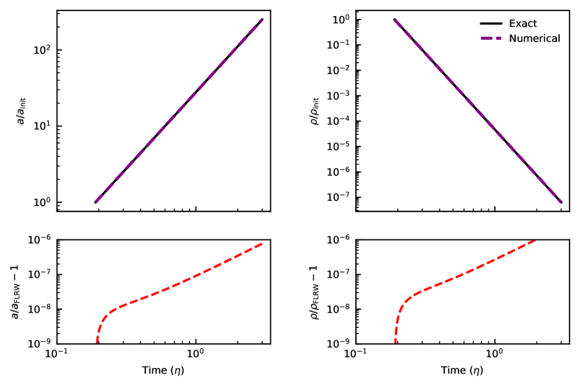
Figure 1: Matter dominated FLRW universe: Comparison between numerical solutions (magenta) and exact solutions (black). The top two plots show the evolution of scale factor (top left) and density (top right), while the bottom plots show the residuals of scale factor (bottom left) and density (bottom right). Simulations were performed with a grid resolution of $32^{3}$ and a particle resolution of $64^{3}$.

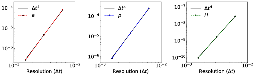
Figure 2: Convergence study of matter dominated FLRW universe: the $L_{1}$ errors for scale factor (left), density (middle) and Hamiltonian constraint (right) are compared to the expected 4th order convergence in time for the RK4 integrator. The circle markers indicate data points from our simulations, while the solid lines are polynomials of the form $\Delta t^{4}$. Our method shows the expected $\mathcal{O}(\Delta t)^{4}$ convergence, for the scale factor, density, and Hamiltonian constraint.

III FLRW spacetime

III.1 Setup

A homogeneous and isotropic FLRW metric in synchronous gauge has the form

$$ds^{2}=a(\eta)^{2}\left[-d\eta^{2}+\frac{1}{(1+kr^{2}/4)^{2}}\delta_{ij}dx^{i}dx^{j}\right],$$ (27)

where $\eta$ is conformal time, $a(\eta)$ is the scale factor, $k$ is the curvature parameter that can take values of $k=0,-1,1$ for a flat, negatively curved or positively curved universe respectively. We initialise a homogeneous and isotropic universe with initial scale factor $a_{\text{init}}=1$ and an initial density $\rho_{\text{init}}$ obtained from solving the Friedmann equation for a matter dominated universe

$$\mathcal{H}_{\text{init}}=\sqrt{\frac{8\pi\rho_{\text{init}}a^{2}_{\text{init}}}{3}},$$ (28)

where $\mathcal{H_{\text{init}}}$ is the initial Hubble rate. We set the spatial metric

$$\gamma_{ij}=a^{2}\delta_{ij},$$ (29)

and the extrinsic curvature via the derivative of the spatial metric

$$\frac{\text{d}}{\text{d}t}\gamma_{ij}=-2\alpha K_{ij},$$ (30)

where $d/dt={\partial}/{\partial t}-\mathcal{L}_{\beta}$ and $\mathcal{L_{\beta}}$ is the Lie derivative in the direction of the shift, which is always zero based on our gauge choice of $\beta^{i}=0$. The extrinsic curvature is therefore

$$K_{ij}=-\frac{\dot{a}{a}}{\alpha}\delta_{ij},$$ (31)

where an over-dot represents a derivative with respect to conformal time. We initialise an FLRW spacetime in einstein toolkit using flrwsolver [17].

To set the initial stress-energy tensor, we first set a uniform cubic lattice of particles with zero velocity, and zero pressure. The particle mass is set by considering the total mass in the domain

$$M=\int\rho^{*}{\rm d}V,$$ (32)

where $\rho^{*}$ is the conserved density and $V$ is the volume of the domain. Since we have a constant density

$$M=\rho^{*}V,$$ (33)

we divide this mass by the total number of particles to obtain the mass of each particle.

By setting zero pressure we see implicitly from Equation 18 that

$$K=0,$$ (34)

$$\frac{{\rm d}K}{{\rm d}t}=0,$$ (35)

and as such we can neglect the calculation of Equation 8 and the evolution of entropy. The stress-energy tensor is then calculated on the particles and interpolated back to the grid as described in Section II.3.3. The kernel interpolation used to obtain the density on each particle introduces a small bias compared to the initial density. In most simulations using SPH, small variations in density compared to the setup are not an issue. However, in our case this manifests as a small violation of the Hamiltonian constraint

$$H\equiv{}^{(3)}R-K_{ij}K^{ij}+K^{2}-16\pi\rho=0,$$ (36)

where ${}^{(3)}R$ is the three-Ricci scalar. We apply the correction factor described in Section II.3.3 to the interpolated stress-energy tensor to fix this, which results in the initial Hamiltonian constraint satisfied to $H\approx 10^{-7}$ in code units. To quantify the smallness of this error, we calculate an order of magnitude estimate of the relative violation via $H_{\rm rel}\approx H/16\pi\rho$. Our initial density in code units is $\rho_{\rm{init}}\approx 13.29$, and thus the relative Hamiltonian constraint violation is $\mathcal{O}\sim 10^{-10}$.

Our choice of gauge in Equation 2 is a harmonic-type slicing which, for an FLRW background, results in the matching of the simulation coordinate time with conformal time.

Give our gauge choice, the evolution of the scale factor for a matter dominated universe is given by

$$a(\eta)\propto\eta^{2},$$ (37)

and the primitive density evolution is given by

$$\rho(\eta)\propto\eta^{-6}.$$ (38)

We initialise our Einstein-de Sitter (EdS) simulation with a $1h^{-1}$Gpc box length at redshift $z_{\rm ini}=1000$, corresponding to a ratio of initial box size to Hubble scale of $\mathcal{H}L\approx 10.55$. This choice sets our initial Hubble expansion and background density in code units, as in [18]. Our initial conformal time is then set via $\eta_{\rm{init}}=2/\mathcal{H}_{\rm{init}}$ and we evolve until the scale factor has increased by a factor of $250$. Time integration is performed with a fourth-order Runge-Kutta method. We used a grid size of $32^{3}$ and a particle resolution of $64^{3}$ particles, corresponding to $8$ particles per grid cell, and choose a box length of $L=1$ in code units.

III.2 Results

Figure 1 shows a comparison of numerical solutions using our $N$-body code to the solutions of the Friedmann equations for a dust FLRW universe. The top two panels show the evolution of scale factor ($a$) and density ($\rho$) relative to their initial values ($a_{\text{init}}$ and $\rho_{\text{init}}$ respectively) with a magenta dashed line. The time evolution for exact solutions for scale factor ($a_{\text{FLRW}}$) and density ($\rho_{\text{FLRW}}$) is shown with a black solid line. Our numerical solutions show agreement with the exact solutions, with residuals (bottom two panels) on the order of $10^{-6}$ for scale factor and $10^{-5}$ for density, even at relatively low grid and particle resolutions.

To quantify the error in our numerical method, and ensure that we demonstrate the expected numerical convergence, we calculate the $L_{1}$ error for scale factor, density, and the Hamiltonian constraint. We calculate the $L_{1}$ error in some quantity $q$ using

$$L_{1}(q)=\frac{1}{nq_{\text{max}}}\sum^{n}_{i=1}\left|q_{i}-q_{\;\text{FLRW}}\right|,$$ (39)

where $q_{\text{FLRW}}$ is the analytic value for an FLRW spacetime of the quantity $q_{i}$ at grid cell $i$, and $q_{\text{max}}$ is the maximum value of the analytic solution within the domain, used for normalisation. We opt for this normalised $L_{1}$ calculation to avoid biasing our error where the exact value is small. Figure 2 shows the $L_{1}$ error in scale factor (left), density (middle), and Hamiltonian constraint (right) for simulations with $\Delta t=0.0015625$, $0.003125$ and $0.00625$ in code units. The filled colour circles represent our data points while the solid black line shows the $\propto\Delta t^{4}$ relationship expected from the truncation error in the timestepping scheme. We see the expected fourth-order convergence for both scale-factor, density, and Hamiltonian constraint.

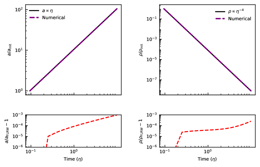
Figure 3: Radiation dominated FLRW universe: top panel, comparison between numerical (magenta) and exact solutions (black) with constant initial density. The evolution of scale factor (left) and density (right) compared to exact solutions is shown in the top two panels. The bottom panel shows the relative errors compared to analytical solutions.

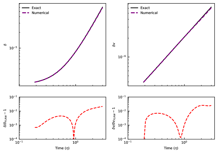
Figure 4: Linearly perturbed matter dominated FLRW universe: comparison between numerical solutions (magenta) and exact solutions (black) with sinusoidal perturbations to initial velocity and density. The evolution of the density perturbation $\delta$ is shown on the top left, while the evolution of the velocity perturbation is shown in the top right. Relative errors for $\delta$ and $\delta v$, are shown on the bottom left and bottom right respectively. The simulation was performed with $64^{3}$ particles and a $32^{3}$ numerical relativity grid.

Figure 5: Convergence study for linear perturbations to a matter dominated FLRW universe: The $L_{1}$ errors of both the density perturbation (left), velocity perturbation (middle) and Hamiltonian constraint (right) are compared to the expected second order convergence. The circle markers indicate points from our simulations, while the expected $\mathcal{O}(\Delta x^{2})$ convergence is shown with the solid black line.

III.3 Radiation Dominated Universe

In addition to a dust FLRW universe, we simulated the evolution of a constant density radiation dominated universe. Once again we initialise a homogeneous and isotropic universe with an initial scale factor and density as described in Section III.1. Unlike our dust universe, we have some pressure via

$$P=w\rho_{\textrm{energy}},$$ (40)

where $w$ is a dimensionless number and $\rho_{\textrm{energy}}$ is the energy density. For an ultra-relativistic (i.e radiation dominated) universe we have

$$P=\frac{1}{3}\rho_{\textrm{energy}},$$ (41)

and $\rho_{\textrm{energy}}=aT^{4}$. We consider an adiabatic equation of state such that

$$P=(\gamma_{\rm ad}-1)\rho u,$$ (42)

where $\gamma_{\rm ad}$ is the adiabatic index and $u$ is the internal energy. Combining Equations 41 and 42, we obtain an adiabatic index of $\gamma_{\rm ad}=4/3$. To set our stress-energy tensor, we initialize a uniform cubic lattice of particles with density $\rho_{\textrm{init}}$, once again obtained from solving the Friedmann equation. We then set an internal energy via

$$u=\frac{aT^{4}}{\rho},$$ (43)

which then sets an initial pressure. We set an initial temperature of $T_{\rm{init}}\approx 6500$K such that our radiation energy density dominates the matter energy density. As we are considering only a constant density radiation dominated universe with no irreversible dissipation, the entropy variable $K$ is constant.

In our chosen gauge, the evolution of the scale factor for a radiation dominated universe is given by

$$a(\eta)\propto\eta,$$ (44)

and the primitive density evolution is given by

$$\rho(\eta)\propto\eta^{-4}.$$ (45)

We begin at $\eta_{\rm init}=1/\mathcal{H}_{\rm init}$ and evolve until $\eta\approx 10$ corresponding to an approximate change in scale factor volume of $100$. Figure 3 shows the evolution of a constant density radiation dominated FLRW universe using our method, compared to the analytic solutions given in Equations 44 and 45. The top panels show the evolution of the scale factor (left) and density (right), with the numerical solutions indicated with the dashed magenta lines, while the analytical solutions are shown by the solid black lines. The bottom two panels show the relative errors in scale factor (left) and density (right) compared to exact solutions. Our numerical solutions show agreement with the exact solutions, to an order of $10^{-3}$ for density and $10^{-4}$ for scale factor even at low grid and particle resolutions. We note that the $L_{1}$ errors obtained for the constant density radiation dominated universe are a few orders of magnitude higher than that of the dust universe. We attribute this to the additional simulation time required to achieve the same change in simulation volume (due to the linear growth of $a$ with $\eta$ from Eq. 44).

IV Linear Perturbations

We introduce small perturbations to the FLRW initial conditions, following the setup of [17] with the thorn flrwsolver. We describe the setup briefly below, for a more complete treatment we refer the reader to [17] or [18]

IV.1 Setup

Writing the metric for an FLRW universe in terms of scalar perturbations only we have

$${\rm d}s^{2}=a^{2}(\eta)\left[(-1+2\psi){\rm d}\eta^{2}+(1-2\phi)\delta_{ij}{\rm d}x^{i}{\rm d}x^{j}\right],$$ (46)

where, in this gauge, $\psi$ and $\phi$ coincide with the Bardeen potentials [66]. Assuming amplitudes such that $\phi,\psi\ll 1$, we can solve Einstein’s field equations using linear perturbation theory, following [17, 18]. Extracting only the growing mode we arrive at the following equations:

$$\phi=f(x^{i}),$$ (47)

$$\delta=\frac{2}{3\mathcal{H}^{2}}\nabla^{2}f(x^{i})-2f(x^{i}),$$ (48)

$$v^{i}=-\frac{2}{3a\mathcal{H}}\delta f(x^{i}),$$ (49)

where we have freedom to choose $f(x^{i})$ provided that it is sufficiently small to retain our linear approximation. Since

$$\mathcal{H}_{\text{init}}=2/{\eta_{\text{init}}},$$ (50)

equations 48 and 49 have an evolution of $\delta\propto\eta^{2}$ and $v^{i}\propto\eta$. We chose $\phi$ of the form

$$\phi=\phi_{0}\sum_{i=1}^{3}\sin\left(\frac{2\pi x^{i}}{\lambda}-\theta\right),$$ (51)

where $\phi_{0}$ is the initial perturbation, $\lambda$ is the wavelength and $\theta$ is the phase offset Using this value of $\phi$, equations 48 and 49 are

$$\delta=-\left[\left(\frac{2\pi}{\lambda}\right)^{2}\frac{a_{\text{init}}}{4\pi\rho^{*}}+2\right]\phi_{0}\sum_{i=1}^{3}\sin\left(\frac{2\pi x^{i}}{\lambda}-\theta\right),$$ (52)

and

$$v^{i}=-\left(\frac{2\pi}{\lambda}\right)^{2}\frac{\mathcal{H}_{\text{init}}}{4\pi\rho^{*}}\phi_{0}\sum_{i=1}^{3}\cos\left(\frac{2\pi x^{i}}{\lambda}-\theta\right),$$ (53)

respectively.

After setting the metric quantities based on the perturbations of density and velocity, we initialise a density distribution by stretching a cubic lattice with the stretch-map method of [67] employing Equation 52 for the density perturbation. We also set particle velocities based on their position and Equation 53. Due to the nature of stretching a finite particle resolution to a given density distribution, we do not exactly recover our initial density and velocity perturbations on the particles, and as such have initial residuals on the order of $10^{-4}$. In principle, provided we have a large enough particle resolution, we obtain residuals that approach machine precision.

We set $\phi_{0}=10^{-6}$ and $\mathcal{H}_{\rm{init}}\approx 10.55$, which corresponds to initial amplitudes of $\delta\approx 10^{-6}$ and $\delta v^{i}\approx 10^{-7}$, and evolve the simulation from $\eta=2/\mathcal{H}_{\rm{init}}$ until $\eta\approx 3$ corresponding to a factor of $\approx 250$ change in scale factor. We perform time integration using a fourth-order Runge-Kutta method.

IV.2 Results

Figure 4 shows the numerical evolution of the amplitude of the density perturbation $\delta$ (left) and maximum velocity perturbation $\delta v$ (right) with dashed magenta curves in the top two panels. We calculate the amplitudes of the perturbations by fitting a sine function to the particle data ($\sin(\theta)$ for $\delta$ and $\cos(\theta)$ for $\delta v$) using scipy.curve_fit. Exact solutions, given by Equations 52 and 53, are shown with solid black curves. The bottom panels show the relative errors for $\delta$ (left) and $\delta v$ (right). As with the constant density simulations of Section III we also quantify our errors by computing the $L_{1}$ error (Equation 39). Figure 5 shows the $L_{1}$ errors in the density perturbation ($\delta$), velocity perturbation ($\delta v$) and Hamiltonian constraint ($H$) for increasing particle resolutions of $16^{3}$, $32^{3}$, and $64^{3}$. All simulations are performed with a grid resolution of $32^{3}$. We see the expected second order convergence with increasing particle number for $\delta$, $\delta v$ and $H$. Our simulations of a linearly perturbed FLRW spacetime show agreement with exact solutions of order $10^{-2}$ by the end of the evolution.

Figure 6: Non-linear one-dimensional perturbation to a matter dominated universe: density (lower) and velocity (upper) perturbations as a function of position, for various values of conformal time $\eta$. The numerical result is given by the dashed magenta curves, while the gray solid curves represent sinusoids with the same amplitude as the numerical result, thus showing the expected deviation from linear solutions. The simulation was performed with a $32^{3}$ numerical relativity grid and $64^{3}$ particles.

Figure 7: Three-dimensional collapse of an overdense region: column integrated density of our simulation at $\eta\approx 1.89$ and $\eta\approx 98$. The simulation was performed with a particle resolution of $32^{3}$ and a grid resolution of $32^{3}$, and exact kernel interpolation.

V Nonlinear Evolution & Shell Crossing

Figure 8: Plane wave collapse of non-linear perturbations: velocity (upper) and density (lower) are shown as a function of position at $\eta\approx 148$ (corresponding to roughly the time of shell crossing), $\eta\approx 304$ and $\eta\approx 357$ (representing points well past shell crossing). We see the formation of a spiral like structure in velocity and of various caustic like spikes in density, as expected after shell crossing even with a relatively low grid resolution of $32^{3}$.

V.1 Setup

To perform a nonlinear evolution, we chose an initial perturbation of $\phi_{0}=10^{-5}$ such that the linear approximation of flrwsolver remains valid. Our initial $\phi_{0}$ gives perturbations in velocity and density of $\delta=10^{-4}$ and $\delta v=10^{-5}$ in the $x$ direction, as shown in Figure 6.

In addition to the $x-$direction-only perturbation, we also evolved a nonlinear simulation with perturbations in $x$, $y$ and $z$ directions. These perturbations are initialised on particles by performing the stretch mapping procedure three times: once for each direction. Velocities are directly specified at each particle position using Equation 53. Once again, we use an initial perturbation of $\phi=10^{-5}$, which gives maximum values of $\delta=10^{-4}$ and $\delta v=10^{-5}$. For both simulations we begin at $\eta_{\rm{init}}\approx 1.89$ and evolve until $\eta\approx 360$. We perform time integration using a second-order Runge-Kutta method. Simulations are performed with a particle resolution of $64^{3}$, and a grid resolution of $32^{3}$ in the one-dimensional perturbation, and the three-dimensional perturbation using both a particle and grid resolution of $32^{3}$.

V.2 Results

Figure 6 shows the velocity (lower) and density (upper) with respect to position at times of $\eta\approx 1.89$ (initial time), $\eta\approx 35$, $\eta\approx 50$ and $\eta\approx 66$. The magenta dashed curves represent the values obtained from our simulations while the solid gray curves show sinusoids of the same amplitude as the numerical solutions. We calculate our sinusoids by fitting a sine function to the particle data ($\sin(\theta)$ for $\delta$ and $\cos(\theta)$ for $\delta v$) using scipy.curve_fit. We see a deviation from the linear (sinusoidal) shape at $\eta\approx 50$ indicating that our simulations have passed into the non-linear regime as expected. Figure 7 shows the column-integrated density perturbation at $\eta\approx 1.89$ and $\eta\approx 98$ in the $x$-$y$ plane for a simulation with perturbations in each direction. The overdense region in the top right-hand corner collapses to a point with a column integrated density perturbation $\approx 88$ times greater than the initial distribution, with a void forming in the bottom left corner.

V.3 Shell Crossing

To explore the impact of shell crossings using our method, we consider initial linear perturbations of $\phi=10^{-5}$, $\delta\approx 10^{-4}$ and $\delta v\approx 10^{-5}$ to FLRW background as in Section V.2. We evolve to $\eta\approx 365$ such that our numerical solutions diverge significantly from the linear solutions and caustic formation occurs. Figure 8 shows the density and velocity distributions as a function of position. We show the density and velocity distributions at shell crossing $\eta\approx 148$, $\eta\approx 304$ and $\eta\approx 357$ representing the evolution well past shell crossing. The spiral shapes shown in velocity, and the caustics in density are characteristic of a shell crossing. We stress that the conformal times shown are not meant to be physically meaningful, and are just indicative of the simulation time required to form such structures. We also continue to evolve our simulation of the three-dimensional perturbation until shell-crossing occurs. Figure 9 shows the distribution of particle $x$ velocity with respect to $x$ position for the three-dimensional perturbation at $\eta\approx 226$. Like the one-dimensional perturbation, we see the emergence of a ‘spiral’ like structure in phase space. To quantify the numerical stability of our simulations, we show the evolution of the Hamiltonian and momentum constraints in Figure 11. while we see an increase in constraint violation once the shell crossing occurs, the evolution remains stable during and beyond this point.

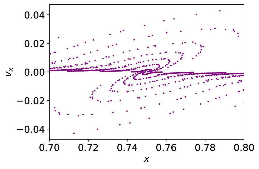
Figure 9: The distribution of particle velocity in the $x$-direction as a function of $x$ position for the simulation of a three-dimensional, non-linear perturbation shown in Figure 7. Here we show a restricted domain corresponding to roughly the position of the ‘dark matter halo’. The system has evolved well past shell crossing and has begun to undergo virialization.

VI Discussion and Conclusions

We have introduced a new method for simulating homogeneous and inhomogeneous cosmologies by coupling the einstein toolkit numerical relativity code to the phantom general relativistic smoothed particle hydrodynamics code. Similar to the works of Macpherson et al. [17, 18], Bentivegna and Bruni [10], and Giblin et al. [20, 19] we have shown that numerical relativity is a viable tool for the simulation of homogeneous and inhomogeneous cosmology, albeit at low resolution. Like [17], our initial conditions extract only the growing mode, rather than both the growing and decaying modes. Unlike the previously stated methods, our method is capable of simulating gravitational collapse without shell crossing singularities, and thus can facilitate the formation of dark matter halos in fully non-linear general relativity.

We demonstrated the evolution of a flat dust FLRW universe with errors of the order of $10^{-6}$ compared to exact solutions, with the expected fourth order convergence caused solely by truncation error in the timestepping scheme, whilst using relatively low particle ($64^{3}$) and grid ($32^{3}$) resolutions. The evolution of linear perturbations to a dust FLRW universe, has relative errors in density and velocity compared to analytical solutions on the order $10^{-2}$, whilst demonstrating the expected second order convergence in space.

Unlike previous attempts to employ N-body particle methods in numerical relativity [27, 26, 28], our method allows for simulation of gas as well as collisionless matter and works in 3D, fully nonlinear general relativity rather than using post-Newtonian approximations [68, 25] or restricted dimensionality [69]. In particular, we also demonstrated the evolution of a flat, radiation-dominated universe with errors on the order of $10^{-3}$ compared to the radiation-dominated FLRW solution.

Finally, we show the evolution of non-linear perturbations in both one-dimensional and three-dimensional perturbations past the point of shell crossing. We follow the formation of dark matter halos without any significant violations in either the Hamiltonian or momentum constraints.

Implementation wise, our main difficulty was our initial attempt to split the timestepping between the two codes, evolving the particle quantities in phantom, while the BSSN equations were evolved in einstein toolkit. We found that the simplest approach was instead to discretise the time derivatives on the left hand side of the fluid equations in einstein toolkit and use phantom to compute the particle summations needed for the density estimate and spatial derivatives on the right hand side.

As in Rosswog and Diener [55], Rosswog et al. [50], Diener et al. [51], we coupled Lagrangian hydrodynamics code to numerical relativity. However, there are several key differences in implementation. Firstly, we use a regular SPH kernel for interpolating the stress-energy tensor back to the grid. This is accompanied by the exact interpolation of Petkova et al. [65] which helps to ensure that mass and momentum are conserved when interpolating from particles to the grid. We also evolve an entropy variable, instead of total energy and as such we do not need to compute time derivatives of the metric.

In this work we have only considered applications to inhomogeneous cosmology. However, there are other applications which could be investigated using our code. The most notable of these is the application to compact binary mergers, however, this would require the development of a fixed mesh refinement method.

Future work could investigate non-linear effects with realistic cosmological initial conditions similar to Macpherson et al. [18]. This would mainly require further optimisation of our code. The current largest bottleneck is the expense of interpolating the stress energy tensor from the particles to the grid, limiting the maximum resolutions we can study in reasonable computation time. Improvements could also be made to the parallelisation, since we are currently limited to one cluster node since our code does not yet support MPI parallelisation.

Throughout this work we have only performed simulations using a single uniform grid, which may not be optimal for studying the formation of dark matter halos in a realistic, large-scale universe simulation. The development of an adaptive mesh refinement method that works in conjunction with the AMR methods implemented in einstein toolkit would be desirable. Our main limitation is the large computational expense compared to traditional Newtonian $N$-Body simulations. The combination of numerical relativity with particles makes the evolution slower than traditional N-body because of the required interpolation at every time step to go from particles to grid and vice versa, which is unavoidable. Despite these limitations, we have shown that simulations of cosmological spacetimes using numerical relativity need no longer be limited by the use of a fluid approximation.

Appendix A Constraint Violation

For some of the simulations presented in this paper we quantified our errors compared to exact solutions by calculating relative errors and also through a calculation of the $L_{1}$ error. For numerical relativity simulations without exact solutions, the error can be quantified by looking at the violations in the constraint equations for the Hamiltonian and momentum constraints

$$H\equiv{}^{(3)}R-K_{ij}K^{ij}+K^{2}-16\pi\rho=0,$$ (54)

$$M_{i}\equiv D_{j}K^{j}_{i}-D_{i}K-S_{i}=0,$$ (55)

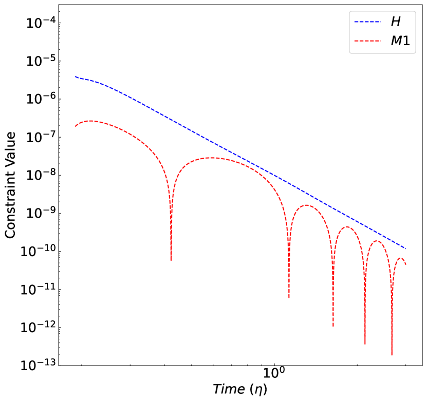
Figure 10: Constraint evolution for a linear perturbation to a matter dominated FLRW universe. The $L_{1}$ error of the Hamiltonian (blue) and momentum (red) constraints are shown with respect to conformal time.

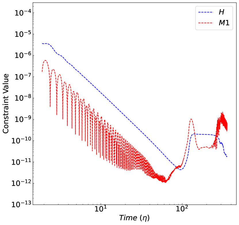
Figure 11: Constraint evolution for a non-linear one-dimensional perturbation to a matter dominated FLRW universe. The $L_{1}$ error of the Hamiltonian (blue) and momentum (red) constraints are shown with respect to conformal time.

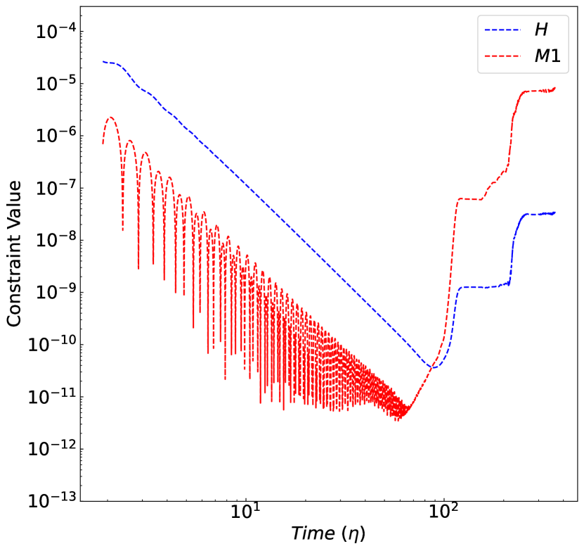
Figure 12: Constraint evolution for a non-linear three-dimensional perturbation to a matter dominated FLRW universe. The $L_{1}$ error of the Hamiltonian (blue) and momentum (red) constraints are shown with respect to conformal time.

where $D_{j}$ is the 3-metric covariant derivative, and $S_{i}=-\gamma_{i\alpha}n_{\beta}T^{ab}$. An initial constraint violation of $\mathcal{O}\sim 2\times 10^{-5}$ in $H$ occurs due to a difference between initial metric quantities and initial densities. This is particularly pertinent when dealing with a density distribution discretised to particles. We have two main sources of error when reconstructing our density distribution. Firstly, we there is a small initial error due to stretching the lattice of particles to our desired density distribution. Secondly we have an error due to the bias of our kernel. Similarly, large increases in constraints during the evolution of our simulations are indicative of departures from numerical stability. Figure 10 shows the time evolution of the Hamiltonian and Momentum constraints for the linear perturbation to a dust FLRW universe. While we show the constraint violations in code units, we can normalise these violations by the order of magnitude of the individual terms to get an insight into the relative violation we are seeing. The maximum density at the end of the simulation in code units is $\rho_{\text{max}}\approx 8\times 10^{-7}$, which gives a relative $H$ violation, $H_{\rm rel}\approx H/16\pi\rho$, of $\mathcal{O}\sim 5\times 10^{-7}$. Note that we did not compute the $L_{1}$ error of the relative constraint violation (see [18]) as this would have required several more quantities to be interpolated to the grid (and corrected) at significant computational expense. Figure 11 shows the evolution of the Hamiltonian and Momentum constraints in the non-linear regime for a one-dimensional perturbation to an FLRW universe. We see increases in Hamiltonian and Momentum constraints at $\eta\approx 100$ as the system undergoes shell crossing, and a increase in the momentum constraint at $\eta\approx 300$ as the virialization begins to occur. However, there is no large increase in constraint values indicative of numerical instability. The relative Hamiltonian constraint is $\mathcal{O}\sim 7\times 10^{-1}$ at the end of the simulation. Finally, Figure 12 shows the time evolution of the Hamiltonian and momentum constraints for a non-linear perturbation in each direction. Like the one-dimensional case we have an increase in both the Hamiltonian and momentum constraints as shell crossing begins to occur at $\eta\approx 100$, before plateauing and increasing as instances of shell crossing reoccur. The maximum density is $\rho_{\text{max}}\approx 2.1\times 10^{-5}$ at the end of the simulation, and thus we obtain a relative Hamiltonian constraint violation of $\mathcal{O}\sim 8\times 10^{-4}$.

References

- Riess et al. [1998] A. G. Riess, A. V. Filippenko, P. Challis, A. Clocchiatti, A. Diercks, P. M. Garnavich, R. L. Gilliland, C. J. Hogan, S. Jha, R. P. Kirshner, B. Leibundgut, M. M. Phillips, D. Reiss, B. P. Schmidt, R. A. Schommer, R. C. Smith, J. Spyromilio, C. Stubbs, N. B. Suntzeff, and J. Tonry, AJ 116, 1009 (1998), arXiv:astro-ph/9805201 [astro-ph] .
- Perlmutter et al. [1999] S. Perlmutter, G. Aldering, G. Goldhaber, R. A. Knop, P. Nugent, P. G. Castro, S. Deustua, S. Fabbro, A. Goobar, D. E. Groom, I. M. Hook, A. G. Kim, M. Y. Kim, J. C. Lee, N. J. Nunes, R. Pain, C. R. Pennypacker, R. Quimby, C. Lidman, R. S. Ellis, M. Irwin, R. G. McMahon, P. Ruiz-Lapuente, N. Walton, B. Schaefer, B. J. Boyle, A. V. Filippenko, T. Matheson, A. S. Fruchter, N. Panagia, H. J. M. Newberg, W. J. Couch, and T. S. C. Project, ApJ 517, 565 (1999), arXiv:astro-ph/9812133 [astro-ph] .
- Brout et al. [2022] D. Brout, D. Scolnic, B. Popovic, A. G. Riess, A. Carr, J. Zuntz, R. Kessler, T. M. Davis, S. Hinton, D. Jones, W. D. Kenworthy, E. R. Peterson, K. Said, G. Taylor, N. Ali, P. Armstrong, P. Charvu, A. Dwomoh, C. Meldorf, A. Palmese, H. Qu, B. M. Rose, B. Sanchez, C. W. Stubbs, M. Vincenzi, C. M. Wood, P. J. Brown, R. Chen, K. Chambers, D. A. Coulter, M. Dai, G. Dimitriadis, A. V. Filippenko, R. J. Foley, S. W. Jha, L. Kelsey, R. P. Kirshner, A. Möller, J. Muir, S. Nadathur, Y.-C. Pan, A. Rest, C. Rojas-Bravo, M. Sako, M. R. Siebert, M. Smith, B. E. Stahl, and P. Wiseman, ApJ 938, 110 (2022), arXiv:2202.04077 [astro-ph.CO] .
- Blake et al. [2011] C. Blake, E. A. Kazin, F. Beutler, T. M. Davis, D. Parkinson, S. Brough, M. Colless, C. Contreras, W. Couch, S. Croom, D. Croton, M. J. Drinkwater, K. Forster, D. Gilbank, M. Gladders, K. Glazebrook, B. Jelliffe, R. J. Jurek, I. H. Li, B. Madore, D. C. Martin, K. Pimbblet, G. B. Poole, M. Pracy, R. Sharp, E. Wisnioski, D. Woods, T. K. Wyder, and H. K. C. Yee, MNRAS 418, 1707 (2011), arXiv:1108.2635 [astro-ph.CO] .
- Ata et al. [2018] M. Ata et al., MNRAS 473, 4773 (2018), arXiv:1705.06373 [astro-ph.CO] .
- Planck Collaboration et al. [2020] Planck Collaboration, N. Aghanim, Y. Akrami, M. Ashdown, J. Aumont, C. Baccigalupi, M. Ballardini, A. J. Banday, R. B. Barreiro, Bartolo, et al., A&A 641, A6 (2020), arXiv:1807.06209 [astro-ph.CO] .
- Riess et al. [2022] A. G. Riess, W. Yuan, L. M. Macri, D. Scolnic, D. Brout, S. Casertano, D. O. Jones, Y. Murakami, G. S. Anand, L. Breuval, T. G. Brink, A. V. Filippenko, S. Hoffmann, S. W. Jha, W. D’arcy Kenworthy, J. Mackenty, B. E. Stahl, and W. Zheng, ApJ 934, L7 (2022), arXiv:2112.04510 [astro-ph.CO] .
- Hogg et al. [2005] D. W. Hogg, D. J. Eisenstein, M. R. Blanton, N. A. Bahcall, J. Brinkmann, J. E. Gunn, and D. P. Schneider, ApJ 624, 54 (2005), arXiv:astro-ph/0411197 [astro-ph] .
- Scrimgeour et al. [2012] M. Scrimgeour et al., Mon. Not. Roy. Astron. Soc. 425, 116 (2012), arXiv:1205.6812 [astro-ph.CO] .
- Bentivegna and Bruni [2016] E. Bentivegna and M. Bruni, Phys. Rev. Lett. 116, 251302 (2016), arXiv:1511.05124 [gr-qc] .
- Buchert [2008] T. Buchert, General Relativity and Gravitation 40, 467 (2008), arXiv:0707.2153 [gr-qc] .
- Buchert and Räsänen [2012] T. Buchert and S. Räsänen, Annual Review of Nuclear and Particle Science 62, 57 (2012), arXiv:1112.5335 [astro-ph.CO] .
- Springel et al. [2005] V. Springel, S. D. M. White, A. Jenkins, C. S. Frenk, N. Yoshida, L. Gao, J. Navarro, R. Thacker, D. Croton, J. Helly, J. A. Peacock, S. Cole, P. Thomas, H. Couchman, A. Evrard, J. Colberg, and F. Pearce, Nature 435, 629 (2005), arXiv:astro-ph/0504097 [astro-ph] .
- Schaye et al. [2015] J. Schaye, R. A. Crain, R. G. Bower, M. Furlong, M. Schaller, T. Theuns, C. Dalla Vecchia, C. S. Frenk, I. G. McCarthy, J. C. Helly, A. Jenkins, Y. M. Rosas-Guevara, S. D. M. White, M. Baes, C. M. Booth, P. Camps, J. F. Navarro, Y. Qu, A. Rahmati, T. Sawala, P. A. Thomas, and J. Trayford, MNRAS 446, 521 (2015), arXiv:1407.7040 [astro-ph.GA] .
- Springel et al. [2018] V. Springel, R. Pakmor, A. Pillepich, R. Weinberger, D. Nelson, L. Hernquist, M. Vogelsberger, S. Genel, P. Torrey, F. Marinacci, and J. Naiman, MNRAS 475, 676 (2018), arXiv:1707.03397 [astro-ph.GA] .
- Vogelsberger et al. [2020] M. Vogelsberger, F. Marinacci, P. Torrey, and E. Puchwein, Nature Reviews Physics 2, 42 (2020), arXiv:1909.07976 [astro-ph.GA] .
- Macpherson et al. [2017] H. J. Macpherson, P. D. Lasky, and D. J. Price, Phys. Rev. D 95, 064028 (2017), arXiv:1611.05447 [astro-ph.CO] .
- Macpherson et al. [2019] H. J. Macpherson, D. J. Price, and P. D. Lasky, Phys. Rev. D 99, 063522 (2019), arXiv:1807.01711 [astro-ph.CO] .
- Giblin et al. [2016a] J. Giblin, John T., J. B. Mertens, and G. D. Starkman, ApJ 833, 247 (2016a), arXiv:1608.04403 [astro-ph.CO] .
- Giblin et al. [2016b] J. T. Giblin, J. B. Mertens, and G. D. Starkman, Phys. Rev. Lett. 116, 251301 (2016b), arXiv:1511.01105 [gr-qc] .
- Munoz and Bruni [2023a] R. L. Munoz and M. Bruni, Phys. Rev. D 107, 123536 (2023a), arXiv:2302.09033 [astro-ph.CO] .
- Munoz and Bruni [2023b] R. L. Munoz and M. Bruni, Classical and Quantum Gravity 40, 135010 (2023b), arXiv:2211.08133 [gr-qc] .
- Barrera-Hinojosa and Li [2020] C. Barrera-Hinojosa and B. Li, J. Cosmology Astropart. Phys. 2020, 007 (2020), arXiv:1905.08890 [astro-ph.CO] .
- Teyssier [2002] R. Teyssier, A&A 385, 337 (2002), arXiv:astro-ph/0111367 [astro-ph] .
- Adamek et al. [2016a] J. Adamek, D. Daverio, R. Durrer, and M. Kunz, J. Cosmology Astropart. Phys. 2016, 053 (2016a), arXiv:1604.06065 [astro-ph.CO] .
- Daverio et al. [2019] D. Daverio, Y. Dirian, and E. Mitsou, J. Cosmology Astropart. Phys. 2019, 065 (2019), arXiv:1904.07841 [astro-ph.CO] .
- East et al. [2018] W. E. East, R. Wojtak, and T. Abel, Phys. Rev. D 97, 043509 (2018), arXiv:1711.06681 [astro-ph.CO] .
- East et al. [2019] W. E. East, R. Wojtak, and F. Pretorius, Phys. Rev. D 100, 103533 (2019), arXiv:1908.05683 [astro-ph.CO] .
- Giblin et al. [2019] J. T. Giblin, J. B. Mertens, G. D. Starkman, and C. Tian, Phys. Rev. D 99, 023527 (2019), arXiv:1810.05203 [astro-ph.CO] .
- Lucy [1977] L. B. Lucy, AJ 82, 1013 (1977).
- Gingold and Monaghan [1977] R. A. Gingold and J. J. Monaghan, MNRAS 181, 375 (1977).
- Price [2012] D. J. Price, Journal of Computational Physics 231, 759 (2012), arXiv:1012.1885 [astro-ph.IM] .
- Kheyfets et al. [1990] A. Kheyfets, W. A. Miller, and W. H. Zurek, Phys. Rev. D 41, 451 (1990).
- Mann [1991] P. J. Mann, Computer Physics Communications 67, 245 (1991).
- Laguna et al. [1993] P. Laguna, W. A. Miller, and W. H. Zurek, ApJ 404, 678 (1993).
- Chow and Monaghan [1997] E. Chow and J. J. Monaghan, Journal of Computational Physics 134, 296 (1997).
- Rosswog [2010a] S. Rosswog, Journal of Computational Physics 229, 8591 (2010a), arXiv:0907.4890 [astro-ph.HE] .
- Siegler and Riffert [2000] S. Siegler and H. Riffert, ApJ 531, 1053 (2000), arXiv:astro-ph/9904070 [astro-ph] .
- Monaghan and Price [2001] J. J. Monaghan and D. J. Price, MNRAS 328, 381 (2001).
- Rosswog [2010b] S. Rosswog, Classical and Quantum Gravity 27, 114108 (2010b).
- Tejeda and Rosswog [2013] E. Tejeda and S. Rosswog, MNRAS 433, 1930 (2013), arXiv:1303.4068 [astro-ph.HE] .
- Nealon et al. [2015] R. Nealon, D. J. Price, and C. J. Nixon, MNRAS 448, 1526 (2015), arXiv:1501.01687 [astro-ph.HE] .
- Bonnerot et al. [2016] C. Bonnerot, E. M. Rossi, G. Lodato, and D. J. Price, MNRAS 455, 2253 (2016), arXiv:1501.04635 [astro-ph.HE] .
- Hayasaki et al. [2016] K. Hayasaki, N. Stone, and A. Loeb, MNRAS 461, 3760 (2016), arXiv:1501.05207 [astro-ph.HE] .
- Oechslin et al. [2002] R. Oechslin, S. Rosswog, and F.-K. Thielemann, Phys. Rev. D 65, 103005 (2002), arXiv:gr-qc/0111005 [gr-qc] .
- Faber et al. [2004] J. A. Faber, P. Grandclément, and F. A. Rasio, Phys. Rev. D 69, 124036 (2004), arXiv:gr-qc/0312097 [gr-qc] .
- Bauswein et al. [2010] A. Bauswein, R. Oechslin, and H. T. Janka, Phys. Rev. D 81, 024012 (2010), arXiv:0910.5169 [astro-ph.SR] .
- Tejeda et al. [2017] E. Tejeda, E. Gafton, S. Rosswog, and J. C. Miller, MNRAS 469, 4483 (2017), arXiv:1701.00303 [astro-ph.HE] .
- Liptai and Price [2019] D. Liptai and D. J. Price, MNRAS 485, 819 (2019), arXiv:1901.08064 [astro-ph.IM] .
- Rosswog et al. [2022] S. Rosswog, P. Diener, and F. Torsello, arXiv e-prints , arXiv:2205.08130 (2022), arXiv:2205.08130 [gr-qc] .
- Diener et al. [2022] P. Diener, S. Rosswog, and F. Torsello, European Physical Journal A 58, 74 (2022), arXiv:2203.06478 [astro-ph.HE] .
- Rosswog et al. [2023] S. Rosswog, F. Torsello, and P. Diener, arXiv e-prints , arXiv:2306.06226 (2023), arXiv:2306.06226 [gr-qc] .
- Rosswog [2010c] S. Rosswog, Journal of Computational Physics 229, 8591 (2010c), arXiv:0907.4890 [astro-ph.HE] .
- Rosswog [2010d] S. Rosswog, Classical and Quantum Gravity 27, 114108 (2010d).
- Rosswog and Diener [2021] S. Rosswog and P. Diener, Classical and Quantum Gravity 38, 115002 (2021), arXiv:2012.13954 [gr-qc] .
- Löffler et al. [2012] F. Löffler, J. Faber, E. Bentivegna, T. Bode, P. Diener, R. Haas, I. Hinder, B. C. Mundim, C. D. Ott, E. Schnetter, G. Allen, M. Campanelli, and P. Laguna, Classical and Quantum Gravity 29, 115001 (2012), arXiv:1111.3344 [gr-qc] .
- Brown et al. [2009] D. Brown, P. Diener, O. Sarbach, E. Schnetter, and M. Tiglio, Phys. Rev. D 79, 044023 (2009), arXiv:0809.3533 [gr-qc] .
- Baumgarte and Shapiro [1998] T. W. Baumgarte and S. L. Shapiro, Phys. Rev. D 59, 024007 (1998), arXiv:gr-qc/9810065 [gr-qc] .
- Shibata and Nakamura [1995] M. Shibata and T. Nakamura, Phys. Rev. D 52, 5428 (1995).
- Price et al. [2018] D. J. Price, J. Wurster, T. S. Tricco, C. Nixon, S. Toupin, A. Pettitt, C. Chan, D. Mentiplay, G. Laibe, S. Glover, C. Dobbs, R. Nealon, D. Liptai, H. Worpel, C. Bonnerot, G. Dipierro, G. Ballabio, E. Ragusa, C. Federrath, R. Iaconi, T. Reichardt, D. Forgan, M. Hutchison, T. Constantino, B. Ayliffe, K. Hirsh, and G. Lodato, PASA 35, e031 (2018), arXiv:1702.03930 [astro-ph.IM] .
- Price and Monaghan [2007] D. J. Price and J. J. Monaghan, MNRAS 374, 1347 (2007), arXiv:astro-ph/0610872 [astro-ph] .
- Courant et al. [1928] R. Courant, K. Friedrichs, and H. Lewy, Mathematische Annalen 100, 32 (1928).
- Monaghan and Lattanzio [1985] J. J. Monaghan and J. C. Lattanzio, A&A 149, 135 (1985).
- Price [2007] D. J. Price, PASA 24, 159 (2007), arXiv:0709.0832 [astro-ph] .
- Petkova et al. [2018] M. A. Petkova, G. Laibe, and I. A. Bonnell, Journal of Computational Physics 353, 300 (2018), arXiv:1710.07108 [astro-ph.IM] .
- Bardeen [1980] J. M. Bardeen, Phys. Rev. D 22, 1882 (1980).
- Price and Monaghan [2004] D. J. Price and J. J. Monaghan, MNRAS 348, 139 (2004), arXiv:astro-ph/0310790 [astro-ph] .
- Adamek et al. [2013] J. Adamek, D. Daverio, R. Durrer, and M. Kunz, Phys. Rev. D 88, 103527 (2013), arXiv:1308.6524 [astro-ph.CO] .
- Adamek et al. [2016b] J. Adamek, M. Gosenca, and S. Hotchkiss, Phys. Rev. D 93, 023526 (2016b), arXiv:1509.01163 [astro-ph.CO] .