observationObservation

Learning in Repeated Multi-Unit Pay-As-Bid Auctions Rigel Galgana Operations Research Center, Massachusetts Institute of Technology, rgalgana@mit.edu, Negin Golrezaei Sloan School of Management, Massachusetts Institute of Technology, golrezaei@mit.edu,

Motivated by Carbon Emissions Trading Schemes, Treasury Auctions, Procurement Auctions, and Wholesale Electricity Markets, which all involve the auctioning of homogeneous multiple units, we consider the problem of learning how to bid in repeated multi-unit pay-as-bid auctions. In each of these auctions, a large number of (identical) items are to be allocated to the largest submitted bids, where the price of each of the winning bids is equal to the bid itself. In this work, we study the problem of optimizing bidding strategies from the perspective of a single bidder.

This problem is challenging due to the combinatorial nature of the action space. We overcome this challenge by focusing on the offline setting, where the bidder optimizes their vector of bids while only having access to the past submitted bids by other bidders. We show that the optimal solution to the offline problem can be obtained using a polynomial time dynamic programming (DP) scheme under which the bidder’s utility is decoupled across units. We leverage the structure of the DP scheme to design online learning algorithms with polynomial time and space complexity under full information and bandit feedback settings. Under these two feedback structures, we achieve an upper bound on regret of $O(M\sqrt{T\log|\mathcal{B}|})$ and $O(M\sqrt{|\mathcal{B}|T\log|\mathcal{B}|})$ respectively, where $M$ is the number of units demanded by the bidder, $T$ is the total number of auctions, and $|\mathcal{B}|$ is the size of the discretized bid space. We accompany these results with a regret lower bound, which match the linear dependency in $M$.

Our numerical results suggest that when all agents behave according to our proposed no regret learning algorithms, the resulting market dynamics mainly converge to a welfare maximizing equilibrium where bidders submit uniform bids. We further show that added competition reduces the impact of strategization and bidders converge more rapidly to a higher revenue and welfare steady state. Lastly, our experiments demonstrate that the pay-as-bid auction consistently generates significantly higher revenue compared to its popular alternative, the uniform price auction. This advantage positions the pay-as-bid auction as an appealing auction format in settings where earning high revenue holds significant social value, such as the Carbon Emissions Trading Scheme.

Keywords. Multi-unit pay-as-bid auctions, Bidding strategies, Regret analysis, Market dynamics.

1 Introduction

Homogeneous multi-unit auctions, a special case of combinatorial auctions, are commonly used to auction off large quantities of identical items, for example in Carbon Emissions Trading Schemes Goulder and Schein (2013), Schmalensee and Stavins (2017), Goldner et al. (2019), US Treasury Auctions Garbade and Ingber (2005), Binmore and Swierzbinski (2000), Procurement Auctions Ausubel and Cramton (2005), and Wholesale Electricity Markets Tierney et al. (2008), Federico and Rahman (2003), Fabra et al. (2006). In these multi-unit auctions, bidders submit a bid vector and then are allocated their goods and charged payments according to the auction format.

Of widespread use are the uniform price and pay-as-bid (PAB) mechanisms. As natural multi-unit generalizations of the second and first price sealed bid auctions, bidders are allocated units in decreasing order of bids and, for each unit won, are charged as payment the lowest winning bid (uniform price) or their own bid (PAB). In this work, we focus on the PAB auction in light of the recent industry and research community-wide push towards first price auctions, which is mainly due to demand for price transparency and ease of revenue management (Deospotakis et al. 2021, Bigler 2019).

Nevertheless, it has been observed that participants find it challenging to determine how to bid effectively in PAB auctions, as highlighted by Porter et al. (2003). Bidders face a fundamental dilemma: larger bids increase their chances of winning units but also lead to higher payments. This predicament is further complicated by the necessity to submit monotone bid vectors. Bidding too conservatively reduces the probability of winning units in subsequent slots, while bidding excessively may inflate the payment.

In this paper, we address the issue of learning optimal bidding strategies in repeated multi-unit PAB auctions. As we will elaborate later, we develop efficient no-regret algorithms that simplify the bidding complexity associated with PAB auctions. Through simulating the market dynamics derived from these learning algorithms, we empirically analyze the equilibria of PAB auctions, which have been poorly understood prior to our research. Our empirical findings demonstrate that in the equilibria resulting from these market dynamics, bidders’ winning bids converge to the same value, thus addressing concerns regarding price fairness in PAB auctions (Binmore and Swierzbinski 2000, Akbarpour and Li 2020).

We also consistently observe high revenue from these equilibria, especially when compared to its uniform price counterpart. In the context of carbon markets, this additional revenue can be invested into clean-up efforts and green technology; see. e.g., phase 4 of the European Union Emissions Trading System (EU-ETS) (Gregor 2023).

1.1 Technical Contributions

New Framework to Study Learning How to Bid in PAB Auctions (Section 2). Let there be $N$ bidders/agents with $M$-unit demand in a PAB auction with $\overline{M}$ supply. Each bidder $n$ is endowed with valuation vector $\bm{v}_{n}=(v_{n,1},\ldots,v_{n,M})\in[0,1]^{M}$ and submits a bid vector $\bm{b}_{n}=(b_{n,1},\ldots,b_{n,M})\in\mathcal{B}^{M}$, where $\mathcal{B}$ is some discretization of $[0,1]$ that represents the set of all possible bids. Agents then receive allocation $x_{n}\in[M]$ and utility $\sum_{m=1}^{x_{n}}(v_{n,m}-b_{n,m})$ according to the PAB auction rule; see Section 2. Repeating this auction across $T$ rounds, each agent’s goal is to minimize their regret with respect to their hindsight, utility maximizing bid vector. Here, we refer to discretized regret as the regret incurred as a function of $M,\mathcal{B},T$ when restricting our bid space to $\mathcal{B}$. Conversely, we refer to continuous regret as the regret incurred as a function of only $M$ and $T$ when optimizing for the discretization error.

Dynamic Programming Scheme for Hindsight Optimal Offline Solution (Section 3). To design low-regret bidding algorithms, we crucially leverage the structure of the hindsight optimal offline solution. In the offline/hindsight problem, the bidder has access to the (historical) dataset of submitted bids by competitors and seeks to find the utility maximizing bid vector on that dataset. (See Roughgarden and Wang (2016), Derakhshan et al. (2022), Golrezaei et al. (2021b), Derakhshan et al. (2021) for works that study similar problems from an auctioneer’s perspective.)

We show that the optimal solution to the offline problem—which is our benchmark in computing the regret of our online learning algorithms—can be solved using a polynomial time Dynamic Programming (DP) scheme. To do so, we make the following key observation: to win $m$ units (or equivalently, slots), an agent $n$ must have at least $m$ bids larger than the smallest $m$ among the largest $\overline{M}$ bids of all other bidders. This observation allows us to devise a DP where in each step of the DP, we decide about the bid for one unit, while considering the externality that this bid will impose on the bids and utilities for other units. This externality is precisely the fundamental tradeoff of PAB auctions aforementioned: bidding too small decreases the probability of winning the current or any subsequent units, however, bidding too large increases the payment of the current and previous units.

Decoupled Exponential Weights Algorithm (Section 4). We present our first set of algorithms to learn in the online setting, in both the full information and bandit feedback regimes. We leverage our DP scheme to obtain decoupled rewards, or reward estimates in the bandit setting, for each unit-bid value pair. In particular, we can obtain an exact expression for the utility estimate for bidding $b_{m}$ for unit $m$ that is independent of $b_{1},\ldots,b_{m-1}$ or $b_{m+1},\ldots,b_{M}$, subject to bid vector monotonicity. This allows us to mimic the exponential weights algorithm on the exponentially large bid space in polynomial time and space complexity. We show that our decoupled exponential weights algorithm (Algorithm 2) achieves time and space complexities of $O(M|\mathcal{B}|T)$ and $O(M|\mathcal{B}|)$ respectively, with discretized regret $O(M^{\frac{3}{2}}\sqrt{T\log|\mathcal{B}|})$; see Theorem 4.1. Optimizing for the discretization error from using finite bid space $\mathcal{B}$, we show that in the full information setting, our algorithm achieves $O(M^{\frac{3}{2}}\sqrt{T\log{T}})$ regret.

Theorem 1.1 (Informal)

Under full information feedback, there exists an algorithm that achieves discretized and continuous regrets $O(M^{\frac{3}{2}}\sqrt{T\log|\mathcal{B}|})$ and $O(M^{\frac{3}{2}}\sqrt{T\log T})$ respectively in the repeated multi-unit PAB auction.

We also analyze the bandit version of our algorithm and show that it achieves discretized regret $O(M^{\frac{3}{2}}\sqrt{|\mathcal{B}|T\log|\mathcal{B}|})$; see Theorem 4.2. Balancing with the discretization error, this algorithm achieves continuous regret of $O(M^{\frac{4}{3}}T^{\frac{2}{3}}\sqrt{\log T})$ (We defer the proofs of these and our other main results to the appendix unless otherwise stated).

Online Mirror Descent Algorithm (Section 5). In this section, we present an alternative learning algorithm based on Online Mirror Descent (OMD) that improves the regret upper bounds of our decoupled exponential weight algorithm by a factor of $\sqrt{M}$ at the cost of additional computation. We once again leverage our DP scheme and in particular the graph induced by the DP (see Section 3 for a formal definition). Given this DP graph, one idea is to maintain probability measures over the edges of the DP graph to learn how to bid. Such an idea, which has been studied in other contexts (see Takimoto and Warmuth (2003), Zimin and Neu (2013), Chen et al. (2013)), leads to a sub-optimal $O(M|\mathcal{B}|\sqrt{T\log|\mathcal{B}|})$ discretized regret and $O(MT^{\frac{3}{4}}\sqrt{\log T})$ continuous regret. We obtain an improved regret bound by making an important observation that the utility of a bid vector depends only on the nodes of the DP graph and not the edges. Leveraging this fact enables us to maintain probability measures over the nodes in the DP graph, rather than its edges, resulting in an algorithm that achieves time and space complexities polynomial in $M,|\mathcal{B}|,T$, with discretized regrets $O(M\sqrt{T\log|\mathcal{B}|})$ and $O(M\sqrt{|\mathcal{B}|T\log|\mathcal{B}|})$ in the full information and bandit settings, respectively. See Theorem 5.3. This algorithm achieves a factor of $\sqrt{M}$ better than the decoupled exponential weights algorithm. Optimizing for the discretization error from $\mathcal{B}$, we show that in the bandit feedback setting, we derive an algorithm that achieves $O(MT^{\frac{2}{3}})$ regret.

Theorem 1.2 (Informal)

Under bandit feedback, there exists an algorithm that achieves discretized and continuous regrets $O(M\sqrt{T\log|\mathcal{B}|})$ and $O(MT^{\frac{2}{3}}\sqrt{\log T})$ respectively in the repeated multi-unit PAB auction.

Regret Lower Bound (Section 6). To complement our discretized regret upper bound, we construct a regret lower bound for the full information setting which matches our upper bound up to a factor of $\sqrt{\log|\mathcal{B}|}$. We do this by constructing two distributions over adversary bid vectors for which any learning agent is guaranteed to incur regret linear in $M$ when trying to learn the optimal bid under these distributions.

1.2 Experimental Results and Managerial Implications

Our experiments yield valuable practical insights for both auction designers and participants. These insights are primarily derived from simulations of PAB market dynamics using the no-regret learning algorithms outlined in our paper. Additionally, we compare these results with the market dynamics of uniform price auctions using the algorithms described in Brânzei et al. (2023). It is important to emphasize that conducting such systematic comparisons was previously challenging due to the inherent difficulty of characterizing equilibria in these auctions prior to our research.

1. Uniform Bidding in PAB Auctions is Optimal. As shown in Figures 2 and 8, the market dynamics consistently yield convergence of the winning bids and largest losing bids to a common price across all bidders. This partially addresses one of the main concerns over the fairness of the PAB auction. That is, while the payment for each unit can be different across units and across bidders, under a reasonable learning and bidding strategy, these payments across units and bidders converge to the same value in the long run.

2. Simplified Bidding Interface is Sufficient for PAB but not for Uniform Price. In a recent trend of bidding simplification and automation (e.g., Aggarwal et al. (2019), Deng et al. (2023), Susan et al. (2023), Lucier et al. (2023)), auctioneers may find it easier to restrict bidders’ demand expressiveness by requiring only a single price and quantity, rather than a vector of bids. As per our previous insight, the bid value convergence of the market dynamics suggest appropriateness of this simplified bidding interface. In contrast, we show that the market dynamics of the uniform price auction converge to a staggered bid vector (Figure 8), suggesting that the simplified bidding interface may significantly damage the uniform price auction’s welfare, revenue, or bidders’ utility.

3. PAB Obtains High Revenue but Slightly Lower Welfare than Uniform Price. From the insights provided by Figure 7, it is evident that the PAB auction surpasses the uniform price auction in terms of revenue generation. However, it slightly lags behind in welfare, though to a lesser extent. Consequently, auctioneers who prioritize revenue (resp. welfare) should favor the PAB (resp. uniform price) auction over uniform price (resp. PAB) auctions.

1.3 Other Related Works

Learning in Auctions. Most of the recent learning-theory-flavored auction design research has either focused on the single unit setting (Han et al. 2020b, Han et al. 2020a, Balseiro et al. 2022), the perspective of the auctioneer setting reserve prices (Morgenstern and Roughgarden 2016, Mohri and Medina 2016, Cai and Daskalakis 2017, Dudík et al. 2017, Kanoria and Nazerzadeh 2014, Golrezaei et al. 2023a, 2021a, Golrezaei et al. 2023b), or uniform price auctions (Mohri and Medina 2013, 2016, Huang et al. 2018, Nedelec et al. 2019, Haoyu and Wei 2020). However, in PAB auctions, as the space of possible bid vectors is exponentially large, the task of learning how to bid optimally in these multi-unit auctions is more challenging, compared with the single unit setting. This is especially true when the number of units demanded is large which necessitates not only low-regret but also tractable algorithms to learn how to bid optimally. In this paper, we contribute to this line of works by proposing a novel framework under which to analyze and derive efficient, low-regret learning algorithms for these inherently combinatorial multi-unit PAB auctions.

PAB Mechanism. There are several multi-unit auction formats that are commonly used in practice; e.g., uniform price (Binmore and Swierzbinski 2000, Burkett and Woodward 2020, Beyhaghi et al. 2021, Goldner et al. 2019), PAB (Pycia and Woodward 2020, Pesendorfer 2000, Baisa and Burkett 2018), Vickrey-Clarke-Groves (VCG) (Dobzinski and Nisan 2007, Ausubel and Milgrom 2006), ascending price (Cramton 1998, Ausubel 2004). The literature is divided as to which auction is appropriate for various settings. For example, while the PAB mechanism has desirable revenue and welfare guarantees compared to the uniform price auction (Pycia and Woodward 2020), the empirical revenue of the two auctions is often comparable (Hortaçsu and McAdams 2010), and some argue that guess-the-clearing-price and other strategic behavior (Heim and Götz 2021) along with collusion (Tierney et al. 2008) can further damage its performance. Furthermore, there are ethical and fairness concerns regarding PAB auctions, as their discriminatory nature implies that agents pay unequally for the same unit. Despite this criticism, and other arguments for (and against) other auction formats (Porter et al. 2003, Cramton et al. 2004, de Keijzer et al. 2013a, Ausubel et al. 2014, Akbarpour and Li 2020), we focus on the PAB mechanism due to the simplicity and transparency of its payment rule, as well as, its widespread use.

The economics literature has only recently addressed several of the questions regarding the equilibria, bidding dynamics, efficiency, and other key properties of multi-unit PAB mechanisms in the static or Bayesian setting. For example, the Bayesian optimal bidding strategy is known for the case of 2-unit demand and supply multi-unit auctions (Nautz 1995), for when valuations follow a class of parametric distributions (Pycia and Woodward 2020), or when the bidders have symmetric valuations (Ausubel et al. 2014). The PAB mechanism is also known to be smooth (Syrgkanis and Tardos 2012), which yields a number of desirable guarantees on the price of anarchy of the auction (Roughgarden 2015), even with the presence of an aftermarket (Babaioff et al. 2022). An additional attractive property of the PAB mechanism is complete transparency of payments, as given one’s allocation, an agent knows precisely how much they will pay. This is in stark contrast to the uniform price auction, where shill bids can inflate payments by artificially increasing demand (Akbarpour and Li 2020).

Relationship to Uniform Price Auctions. The uniform price auction is an alternative mechanism of allocating multiple homogeneous goods. Closely related to the PAB auction, bidders are allocated units in decreasing order of bids, but instead of charging each bidder their corresponding winning bid, each bidder instead pays the smallest winning bid. The EU-ETS carbon license auctions use the uniform price auction, rather than the PAB auction, largely due to fairness considerations, as each agent pays the same amount per unit allocated (EEX 2023). However, our work shows that price fairness is not a concern in the long term when bidders learn how to bid and converge to a common price.

In a study closely aligned with our research, Brânzei et al. (2023) investigated the problem of learning optimal bidding strategies in multi-unit uniform pricing auctions. Since the uniform price auction employs a distinct payment rule, the bid optimization problem necessitates different approaches compared to the PAB auction. While Brânzei et al. (2023) reformulated the offline bid optimization problem as a path weight maximization problem over a directed acyclic graph (DAG), the construction of these DAGs differs fundamentally from those we constructed in our manuscript for PAB auctions. We also emphasize that the decoupling of utility across units is unique to the PAB setting, which enables improved regret guarantees. Consequently, the path kernel-based algorithms described in Brânzei et al. (2023) for both the full and bandit settings yield sub-optimal regret in terms of dependence on the number of units in the PAB mechanism. As previously mentioned, we introduce an alternative method based on OMD, which achieves regret matching the lower bound.

Structured Bandits. The crux of our paper is constructing time and space efficient no-regret bandit algorithms for bid optimization under a combinatorially large bid space for identical multi-unit PAB auctions. As such, naive implementations of bandit algorithms, such as Exp3, that consider each bid vector as its own arm in isolation incur exponential regret, computational and memory costs. It is similarly difficult to generalize existing efficient cross-learning based algorithms in the single-unit case (Han et al. 2020a, Han et al. 2020b, Badanidiyuru et al. 2021). To combat this, we take from the expansive structured bandit literature, which includes linear bandits (Dani et al. 2008, Abbasi-yadkori et al. 2011, Chu et al. 2011, Lattimore and Szepesvári 2020) and combinatorial bandits (Chen et al. 2013, Audibert et al. 2011, Niazadeh et al. 2022), and convex uncertainty set bandit (Van Parys and Golrezaei 2023). In particular, our algorithm most closely resembles existing algorithms exploiting both these combinatorial and linear aspects in episodic Markov Decision Processes (Zimin and Neu 2013) or cost minimization on graphs (Takimoto and Warmuth 2003). The primary difference is that our algorithm seeks to minimize the sum of the costs of nodes in a path, rather than the edges. We describe how to efficiently perform negentropy regularized OMD updates in our setting.

Multi-Agent Learning. While we seek to derive efficient, low-regret algorithms for a single bidder, as we also explored, it is equally important to understand the implications of the bidding dynamics induced by such adaptive behavior. For example, it may be possible for these adaptive agents to learn to collude (Hendricks and Porter 1989, Pesendorfer 2000, Aoyagi 2003, Calvano et al. 2021, Heim and Götz 2021) which can significantly reduce revenue and welfare. Precisely how much they do so is characterized in the Bayesian setting as the Price of Anarchy (PoA) (Lucier and Borodin 2009, de Keijzer et al. 2013a, Hartline et al. 2014, Roughgarden et al. 2017). The auction efficiency in the dynamic setting is less well understood, though there have been several results for specific auctions and learning algorithms (Blum et al. 2008, Lykouris et al. 2016, Hartline et al. 2015, Golrezaei et al. 2020, Kolumbus and Nisan 2022). However, most of the standard learning theory literature takes the perspective of the auctioneer who optimizes revenue through reserves or supply. More standard in literature is assuming that the auctioneer is an adaptive agent themselves, optimizing over the set of reserves or supply (Mohri and Medina 2013, Roughgarden and Wang 2016, Mohri and Medina 2015). This line of work is closely related to the vast and rapidly growing literature on multi-agent learning (Phelps et al. 2008, Buşoniu et al. 2010, Yang and Wang 2020, Golrezaei et al. 2020, Golrezaei et al. 2023b, Zhang et al. 2021).

The multi-agent learning dynamics in the PAB auction (and also uniform price auction) is studied in our experiments section. To our knowledge, these experiments are the first systematic comparison between the equilibria of PAB and uniform price auctions, showing a noticeable revenue improvement of the PAB over the uniform price auction.

2 Preliminaries

Notation. We let $|\mathcal{S}|$ denote the size of set $\mathcal{S}$, and define $[k]=\{1,\ldots,k\}$ to be the set of the first $k$ positive integers. We define $\mathcal{S}^{+k}$ to be the set of non-increasing $k$-vectors of elements from set $\mathcal{S}$. Similarly, $\mathcal{S}^{-k}$ denotes the set of non-decreasing $k$-vectors of elements from set $\mathcal{S}$. We let $\Delta(\mathcal{S})$ denote the set of valid probability measures over set $\mathcal{S}$. We also say that the quantity $x$ is $\lesssim$, $\propto$, or $\gtrsim$ than $f(a_{1},\ldots,a_{k})$ some function of $k$ algorithm parameters if $x\in\mathcal{O}(f(a_{1},\ldots,a_{k}))$, $x\in\Theta(f(a_{1},\ldots,a_{k}))$, or $x\in\Omega(f(a_{1},\ldots,a_{k}))$, respectively.

Auction format: Pay-as-bid. Consider a scenario in which there are $N$ bidders and $\overline{M}$ identical units available for auction in a PAB format. In this context, we assume that each agent $n$ within the set $[N]$ desires a maximum of $M$ units. (It should be noted that our results can be extended to a situation where each agent $n$ may demand a different maximum number of units, denoted by $M_{n}$, which are not necessarily identical.)

Let $\bm{v}_{n}=(v_{n,m})_{m\in[M]}\in[0,1]^{+M}$ represent agent $n$’s non-increasing marginal valuation profile. This implies that for any given $n$ in the set $[N]$, the following conditions hold: (i) valuation monotonicity $v_{n,1}\geq v_{n,2}\geq\ldots\geq v_{n,M}$ and (ii) the total valuation of agent $n$ after receiving $m$ units is given by $\sum_{k=1}^{m}v_{n,k}$.

Let $\bm{b}_{n}=\{b_{n,m}\}_{m\in[M]}\in[0,1]^{+M}$ represent the non-increasing bids submitted by bidder $n$. Here, $b_{n,m}$ refers to the bid made by bidder $n$ for the $m$-th slot or, equivalently, the $m$-th unit. Similar to $\bm{v}_{n}$, we have the following conditions for any $n\in[N]$: (i) bid monotonicity $b_{n,1}\geq b_{n,2}\geq\ldots\geq b_{n,M}$ and (ii) individual rationality (IR) $b_{n,m}\leq v_{n,m}$ for all $m\in[M]$. It is important to note that the bid monotonicity condition is not an assumptions; it is implied by the auction rule that will be stated shortly. Consequently, the total payment made by bidder $n$ after receiving $m$ units is given by $\sum_{k=1}^{m}b_{n,k}$. We define $\bm{b}_{-n}=(b_{-n,m})_{m\in[\overline{M}]}\in[0,1]^{-\overline{M}}$ as the set of the $\overline{M}$ largest bids not belonging to agent $n$, arranged in increasing order (i.e., $b_{-n,1}\leq\ldots\leq b_{-n,\overline{M}}$).

The auction operates according to the following rules: In a PAB auction, all bids submitted across the $N$ bidders are arranged in descending order. The $m$-th unit is assigned to the bidder with the $m$-th highest bid, and they are charged the amount of their bid. We denote the allocation to agent $n$ as $x_{n}(\bm{b}_{n})=x(\bm{b}_{n},\bm{b}_{-n})$, and the (quasi-linear) utility as $\mu_{n}(\bm{b}_{n})=\mu(\bm{b}_{n},\bm{b}_{-n})$, where

$$x(\bm{b}_{n},\bm{b}_{-n})=\sum_{m=1}^{M}\textbf{1}_{b_{n,m}\geq b_{-n,m}}\quad\text{and}\quad\mu(\bm{b}_{n},\bm{b}_{-n})=\sum_{m=1}^{x_{n}(\bm{b}_{n})}(v_{n,m}-b_{n,m})\,.$$ (1)

respectively. Here, $b_{-n,m}$ represents the $m$-th smallest bid among the $\overline{M}$ largest bids of all other bidders except bidder $n$. It should be noted that $x(\bm{b}_{n},\bm{b}_{-n})$ denotes the number of units that agent $n$ receives in the auction. In the case of tied bids, we assume the use of an arbitrary, publicly known deterministic tie-breaking rule, denoted as $\textsc{TieBreak}_{n}:\mathcal{R}^{+M}\times\mathcal{R}^{-\overline{M}}\to[M]$, to determine the allocation for agent $n$. This tie-breaking rule is incorporated into the allocation as $x(\bm{b}_{n},\bm{b}_{-n})=\sum_{m=1}^{M}\textbf{1}_{b_{n,m}>b_{-n,m}}+\textsc{TieBreak}_{n}(\bm{b}_{n},\bm{b}_{-n})$, and we use this shorthand notation in Equation (1).

Online/Repeated Setting. Consider a repeated setting where the PAB auction is conducted over $T$ rounds. In this repeated setting, we will focus on the perspective of agent $n\in[N]$ and remove additional indexing when it is evident from the context. For each auction round, agent $n$ has a fixed valuation profile represented by $\bm{v}=(v)_{m\in[M]}\in[0,1]^{+M}$, and their bid vector in the $t$-th auction is denoted by $\bm{b}^{t}=(b^{t}_{m})_{m\in[M]}\in[0,1]^{+M}$. Similarly, $\bm{b}^{t}_{-}=(b^{t}_{-m})_{m\in[\overline{M}]}\in[0,1]^{-\overline{M}}$ represents the competing bids in round $t$. In each round, agent $n$ receives $x^{t}_{n}(\bm{b}^{t})$ units and earns a utility of $\mu^{t}_{n}(\bm{b}^{t})$, where:

$$x^{t}_{n}(\bm{b}^{t})=x(\bm{b}^{t},\bm{b}^{t}_{-})\quad\text{and}\quad\mu^{t}_{n}(\bm{b}^{t})=\mu(\bm{b}^{t},\bm{b}^{t}_{-})\,.$$ (2)

Recall that functions $x$ and $\mu$ are defined in Equation (1). The goal of agent $n$ is to choose a sequence of bid vectors $(\bm{b}^{t})_{t\in[T]}$ that maximizes their total utility, given by $\sum_{t=1}^{T}\mu^{t}_{n}(\bm{b}^{t})$. However, the main challenge is that the vectors $\bm{b}^{t}_{-}$, representing the competing bids, are not known in advance. Instead, they are revealed in an online manner. Consequently, agents must learn how to bid optimally throughout the sequence of auctions, taking into account their previous allocations $H^{t-1}=(x^{\tau}(\bm{b}^{\tau}))_{\tau\in[t-1]}$ and their valuation profile $\bm{v}$. The performance of an agent’s learning strategy is evaluated in terms of regret, which quantifies the difference between their expected utility using their learning strategy and the optimal utility achievable with perfect knowledge of the competing bidding vectors in hindsight:

$$\textsc{Regret}=\max_{\bm{b}\in[0,1]^{+M}}\sum_{t=1}^{T}\mu^{t}_{n}(\bm{b})-\mathbb{E}\left[\sum_{t=1}^{T}\mu^{t}_{n}(\bm{b}^{t})\right]\,.$$ (Continuous Regret)

Here, $\bm{b}^{t}_{-}$ can be selected by an adaptive adversary; i.e. an adversary who can select $\bm{b}^{t}_{-}$ as a function of the entire auction history, which includes $\bm{b}^{1},\ldots,\bm{b}^{t-1}$, but does not have access to the possible randomness when selecting $\bm{b}^{t}$. One example is when the other competitors are also behaving according to no-regret learning algorithms. We note that it is known that the time averaged iterates in the game dynamics induced by agents running no-regret learning algorithms converges to a coarse correlated equilibrium (CCE), which have desirable revenue and welfare guarantees via smooth-auction PoA analysis (de Keijzer et al. 2013b, Feldman et al. 2017). As few theoretical results are known regarding the structure of CCE’s in PAB auctions, we hope our proposed algorithms and experiments will provide useful insights in this direction. We will discuss this further in Section 7.

The benchmark, $\max_{\bm{b}\in[0,1]^{M}}\sum_{t=1}^{T}\mu^{t}_{n}(\bm{b})$ used in the definition of continuous regret, is constructed considering all possible $\bm{b}^{t}_{-}$ for every round $t\in[T]$, where in the hindsight optimal solution, the bid vector can be chosen from any vector $\bm{b}\in[0,1]^{+M}$. However, in practice, bid vectors are often restricted to a discretization of $[0,1]$ denoted by $\mathcal{B}=(B_{1},\ldots,B_{|\mathcal{B}|})$, where $0=B_{1}<\ldots<B_{|\mathcal{B}|}=1$. For such cases, we define an analogous version of regret:

$$\textsc{Regret}_{\mathcal{B}}=\max_{\bm{b}\in\mathcal{B}^{+M}}\sum_{t=1}^{T}\mu^{t}_{n}(\bm{b})-\mathbb{E}\left[\sum_{t=1}^{T}\mu^{t}_{n}(\bm{b}^{t})\right]\,.$$ (Discretized Regret)

In both the definitions of continuous and discretized regret, we henceforth implicitly assume that $b_{m}\leq v_{m}$ for any $m\in[M]$; that is, we have the bid vector $\bm{b}$ is subject to individual rationality and overbidding is not allowed. Observe that the benchmark in defining $\textsc{Regret}_{\mathcal{B}}$ is weaker than that in Regret. Nevertheless, they are not too far from each other as we discuss in the following sections. We wish to derive a learning algorithm that achieves an upper bound on Regret that is polynomial in $M$ and sub-linear in $T$. To do so, we consider the discretized setting, and bound $\textsc{Regret}_{\mathcal{B}}$; an upper bound on Regret will be obtained by accounting for the discretization errors.

We consider two feedback structures: (i) full information and (ii) bandit. In the full information setting, the agent’s allocation and the values of $\bm{b}^{t}_{-}$ are revealed after the end of each round, whereas in the bandit setting, only the agent’s allocation is revealed.

3 Hindsight Optimal Offline Solution

In the offline setting, our goal is to determine agent $n$’s optimal fixed bidding strategy for the $T$ rounds of PAB auctions. Recall the following optimization problem with bid space $\mathcal{B}$:

$$\max_{\bm{b}\in\mathcal{B}^{+M}}\sum_{t=1}^{T}\mu^{t}_{n}(\bm{b})\,,$$ (Offline)

where $\mu^{t}_{n}(\bm{b})$ (defined in Equation (2)) represents the utility of agent $n$ in round $t$ given bid vector $\bm{b}$ and competing bids $\bm{b}_{-}^{t}$. As mentioned earlier, the solution to this optimization problem serves as a benchmark for evaluating the performance of online learning algorithms in the repeated setting. Furthermore, it provides valuable insights for designing algorithms with polynomial time and space complexity for the repeated setting.

To solve Problem (Offline), we take advantage of the following decomposition:

$$\sum_{t=1}^{T}\mu^{t}_{n}(\bm{b}) =\sum_{t=1}^{T}\sum_{m=1}^{M}(v_{m}-b_{m})\textbf{1}_{b_{m}\geq b_{-m}^{t}}=\sum_{m=1}^{M}\sum_{t=1}^{T}(v_{m}-b_{m})\textbf{1}_{b_{m}\geq b_{-m}^{t}}$$ (3)

$$:=\sum_{m=1}^{M}\sum_{t=1}^{T}w_{m}^{t}(b_{m}):=\sum_{m=1}^{M}W^{T+1}_{m}(b_{m})\,,$$ (4)

where $w^{t}_{m}(b)=\textbf{1}_{b\geq b^{t}_{-m}}(v_{m}-b)$ represents the utility in the $t$-th auction for winning the $m$-th item with bid $b$, and $W^{T+1}_{m}(b)=\sum_{t=1}^{T}w^{t}_{m}(b)$ represents the cumulative utility gained from winning the $m$-th item with bid $b$ across the $T$ auctions. (Here, in $w^{t}_{m}(b)$, the same tie-breaking rule in Equation (1) is applied). To solve Problem (Offline), we develop a polynomial-time DP scheme utilizing these $w^{t}_{m}(b)$ and $W^{T+1}_{m}(b)$. In particular, for any $m\in[M]$ and any bid $b\in\mathcal{B}$, let $U_{m}(b)$ be the optimal cumulative utility of the agents from units $m,m+1,\ldots,M$ over $T$ auctions assuming that bids for unit $m$ is less than or equal to $b$.

We then have

$$U_{m}(b)=\max_{b^{\prime}\leq b,b^{\prime}\in\mathcal{B}}\left\{W_{m}^{T+1}(b^{\prime})+U_{m+1}(b^{\prime})\right\}\quad b\in\mathcal{B},m\in[M]\quad\text{and}\quad U_{M+1}(b)=0\quad b\in\mathcal{B}\,.$$ (5)

Algorithm 1 uses the aforementioned DP scheme to devise an optimal solution to Problem (Offline). The following theorem, proven in Section 9.1, shows the optimality of Algorithm 1.

Theorem 3.1

Algorithm 1 returns the optimal solution to problem (Offline) with time and space complexity of $O(M|\mathcal{B}|^{2})$ and $O(M|\mathcal{B}|)$ respectively.

Input: Valuation $\bm{v}$ for $\bm{v}\in[0,1]^{+M}$, Other bids $\{\bm{b}^{t}_{-}\}_{t\in[T]}$ for $\bm{b}^{t}_{-}\in\mathcal{B}^{-\overline{M}}$.

Output: Optimal bid vector $\bm{b}^{*}=\text{argmax}_{\bm{b}\in\mathcal{B}^{M}}\mu^{T}_{n}(\bm{b})$ and its corresponding utility.

Let $W^{T+1}_{m}(b)\leftarrow\sum_{t=1}^{T}\textbf{1}_{b\geq b^{t}_{-m}}(v_{m}-b)$, $b\in\mathcal{B},m\in[M]$, define $U_{M+1}(b)\leftarrow 0$, $b\in\mathcal{B}$, and set $b^{*}_{0}=\max(\mathcal{B})$;

for $m\in[M,\ldots,1],b\in\mathcal{B}:U_{m}(b)\leftarrow\text{max}_{b^{\prime}\in\mathcal{B};b^{\prime}\leq b}W^{T+1}_{m}(b^{\prime})+U_{m+1}(b^{\prime})$;

for $m\in[1,\ldots,M]:b_{m}^{\star}\leftarrow\arg\max_{b\leq b_{m-1}^{*}}U_{m}(b)$;

Return $U_{1}(\max(\mathcal{B}))$ and $\bm{b}^{*}=(b_{m}^{*})_{m\in[M]}$.

ALGORITHM 1 Offline$(\bm{v},\{\bm{b}^{t}_{-}\}_{t\in[T]})$

This algorithm to solve the offline bid optimization problem enables us to compute the hindsight optimal utility, which serves as a benchmark for evaluating the effectiveness of our online learning algorithms. It is worth mentioning that we can represent our DP algorithm as an equivalent graph with $M$ layers, with $|\mathcal{B}|$ nodes in each. More precisely, we define the (offline) DP graph as follows:

1. DP nodes/states. There are $M$ layers, each with $|\mathcal{B}|$ nodes in each, denoted by $\{(m,b)\}_{m\in[M],b\in\mathcal{B}}$.

2. DP edges. In this graph, there are only (directed) edges between two consecutive layers, i.e., from layer $m$ to layer $m+1$ for any $m\in[M-1]$. In particular, node $(m,b)$ only has an edge to node $(m+1,b^{\prime})$ for $b^{\prime}\leq b$ and if $b^{\prime}\leq v_{m+1},b\leq v_{m}$.

3. DP weights. We define the weight of node/state $(m,b)$ to be $W_{m}^{T+1}(b)=\sum_{\tau=1}^{T}\textbf{1}_{b\geq b^{\tau}_{-m}}(v_{m}-b)$.

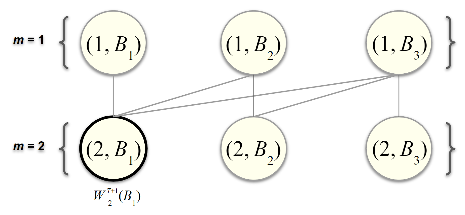
Figure 1: DP graph for problem (Offline): Bid optimization problem cast as a graph problem, for $m=2$ and $|\mathcal{B}|=3$ with $B_{1}<B_{2}<B_{3}$. Node $(m,b)$—the node in the $m$’th layer with bid value $b$—has weight $W_{m}^{T+1}(b)$.

For the online setting, we also note that we can define the DP graph at time $t$, as opposed to $T$, by setting $W_{m}^{t}(b)=\sum_{\tau=1}^{t-1}\textbf{1}_{b\geq b^{\tau}_{-m}}(v_{m}-b)$. This allows us to construct algorithms for the full information and bandit settings by taking advantage of the structure of the DP graph to enhance efficiency and optimize storage of necessary computations.

4 Decoupled Exponential Weights Algorithms

In this section, we present our first algorithm for learning in the online setting. In particular, we construct a decoupled version of the Exponential Weights algorithm which circumvent the large space and time complexity of maintaining and updating the sampling distributions of all possible bid vectors. Our algorithms instead sequentially sample a singular bid value from each layer of our DP graph such that the probability of sampling a particular vector of bids $\bm{b}^{t}$ is precisely equal to the probability of the exponential weights algorithm selecting $\bm{b}^{t}$.

In the following sections, we provide a description of our algorithm in both the full information and the bandit settings. It is important to note that our decoupled exponential weights algorithm achieves regret that is sub-optimal by a factor of $O(\sqrt{M})$. Nonetheless, we present an alternative regret optimal algorithm based on OMD in a subsequent section. Despite this, our decoupled exponential weights algorithm remains practical as it does not necessitate solving a convex optimization problem at each time step $t\in[T]$.

4.1 Full Information Setting

Now let us focus on learning optimal bidding in an online fashion with full information feedback. One straightforward approach in this context is to apply the exponential weights algorithm (Littlestone and Warmuth 1994) to the entire set of bid vectors. This algorithm guarantees per-round rewards within the range of $[-M,M]$. However, the challenge lies in the exponentially large bid space $\mathcal{B}^{+M}$. Tracking and updating weights for all possible bid vectors naively would lead to a non-polynomial time and space complexity. Although this approach achieves a small regret of $O(M^{\frac{3}{2}}\sqrt{T\log|\mathcal{B}|})$, we need a more efficient solution with a polynomial time and space complexity.

To do so, we leverage the DP scheme developed in Section 3. By utilizing the DP graph and the information it provides about bid vector utilities, we can effectively mimic the exponential weights algorithm without explicitly tracking weights for every bid vector. In Algorithm 2, instead of associating weights to each possible bid vector, we associate weights with each $(m,b)$ pair for any $m\in[M]$ and $b\in\mathcal{B}$. These weights are then updated via variables $S_{m}^{t}(b)$ for $b\in\mathcal{B},m\in[M]$, which are inspired by the DP scheme. For any round $t$, we define

$$S^{t}_{m}(b) =\exp(\eta W_{m}^{t}(b))\sum_{\bm{b}^{\prime}_{m+1:M}\in\mathcal{B}^{+(M-m)},b^{\prime}_{m+1}\leq b^{\prime}_{m}=b}\exp(\eta\sum_{m^{\prime}=m+1}^{M}W_{m^{\prime}}^{t}(b^{\prime}_{m^{\prime}}))$$

$$=\exp(\eta W_{m}^{t}(b))\sum_{b^{\prime}\in\mathcal{B};b^{\prime}\leq b}S_{m+1}(b^{\prime})\,.$$

Here, $\eta>0$ is the learning rate of the algorithm and we recall that $W_{m}^{t}(b)=\sum_{\tau=1}^{t-1}w^{\tau}_{m}(b)$ is cumulative utility gained across the first $t-1$ auctions from the winning the $m$’th item with bid $b$, respectively. Computing $S_{m}^{t}(\cdot)$ is done in step $\textsc{Compute}-S_{m}$ of the algorithm. In step $\textsc{Sample}-\bm{b}$, the bid vector is then sampled according to $S_{m}^{t}$’s subject to bid monotonicity. To disallow overbidding, we initialize weights $W^{0}_{m}(b)=-\infty$ for all $m\in[M],b\in\mathcal{B}$ such that $b>v_{m}$.

The concept of utility decoupling shares similarities with solutions used in combinatorial bandits, tabular reinforcement learning (Chen et al. 2013, Zimin and Neu 2013), and problems such as shortest path algorithms involving weight pushing or path kernels (Takimoto and Warmuth 2003, Koolen et al. 2010). These methods are employed to solve variants of the shortest path or maximum weight path problems, where costs or weights are associated with edges rather than nodes. By exploiting the graph structure and the linearity of utilities with respect to the weights of each edge, these algorithms efficiently compute path weights based on edge weights, similar to how our algorithm computes path weights based on node weights. In addition to investigating a fundamentally different problem, the key distinction is that our approach considers weights associated with nodes instead of edges. In our setting, the reward associated with selecting bid $b^{\prime}$ in slot $m+1$ is independent of selecting bid $b\geq b^{\prime}$ in slot $m$. This allows us to get an improved regret bound and save a factor of $|\mathcal{B}|$ in terms of time and space complexity. Instead of storing and updating weights for $O(M|\mathcal{B}|^{2})$ possible $(m,b,b^{\prime})$ slot-value-next value triplets, we only need to handle $O(M|\mathcal{B}|)$ possible $(m,b)$ unit-bid pairs.

The following statement is the main result of this section.

Theorem 4.1 (Decoupled Exponential Weights: Full Information)

With $\eta=\Theta(\sqrt{\frac{\log|\mathcal{B}|}{MT}})$, Algorithm 2 achieves (discretized) regret $O(M^{\frac{3}{2}}\sqrt{T\log|\mathcal{B}|})$, with total time and space complexity polynomial in $M$, $|\mathcal{B}|$, and $T$. Optimizing for discretization error from restricting the bid space to $\mathcal{B}$, we obtain a continuous regret of $O(M^{\frac{3}{2}}\sqrt{T\log T})$.

It is worth noting that both the time and space complexity exhibit polynomial scaling with $M$ and $|\mathcal{B}|$. Given that $M$ can be large in practical scenarios, such as carbon emissions license auctions or electricity markets, it becomes crucial to minimize the dependence on $M$.

Input: Learning rate $0<\eta<\frac{1}{M}$, $\bm{v}\in[0,1]^{+M}$.

Output: The aggregate utility $\sum_{t=1}^{T}\mu_{n}^{t}(\bm{b}^{t})$

$W_{m}^{0}(b)\leftarrow 0$ for all $m\in[M],b\in\mathcal{B}$ such that $b\leq v_{m}$; else $W_{m}^{0}(b)\leftarrow-\infty$;

$b_{0}^{t}\leftarrow\max\mathcal{B}$, and $S_{M+1}^{t}(\min\mathcal{B})=1$ for any $t\in[T]$;

for $t\in[1,\ldots,T]$: do

       Recursively Computing Exponentially Weighted Partial Utilities $\bm{S}^{t}$;

       for $m\in[M,\ldots,1],b\in\mathcal{B}:S^{t}_{m}(b)\leftarrow\exp(\eta W_{m}^{t}(b))\sum_{b^{\prime}\leq b}S_{m+1}^{t}(b^{\prime})$. $\backslash\backslash$ $\textsc{Compute}-S_{m}$;

       Determining the Bid Vector $\bm{b}^{t}$ Recursively;

       for $m\in[1,\ldots,M],b\leq b_{m-1}^{t}:b_{m}^{t}\leftarrow b$ with probability $\frac{S^{t}_{m}(b)}{\sum_{b^{\prime}\leq b_{m-1}^{t}}S^{t}_{m}(b^{\prime})};$   $\backslash\backslash$ $\textsc{Sample}-\bm{b}$;

       Observe $\bm{b}^{t}_{-}$ and receive reward $\mu_{n}^{t}(\bm{b}^{t})$;

       Update Weight Estimates ;

       for $m\in[M],b\in\mathcal{B}:W^{t+1}_{m}(b)\leftarrow W^{t}_{m}(b)+(v_{m}-b)\textbf{1}_{b\geq b^{t}_{-m}}$ if $b\leq v_{m}$; else $W^{t+1}_{m}(b)\leftarrow-\infty$;

      

end for

Return $\sum_{t=1}^{T}\mu_{n}^{t}(\bm{b}^{t})$

ALGORITHM 2 Decoupled Exponential Weights - Full Information

4.2 Bandit Feedback Setting

We extend Algorithm 2 for the bandit feedback setting. In the bandit feedback setting, the bidder’s allocation and utility are not available for all possible bid vectors, unlike in the full information setting. Instead, the agent only observes their utility for the submitted bid vector. To handle this, we use inverse probability weighted (IPW) node weight estimates $\widehat{w}^{t}_{m}(b)$ instead of the node weights $w^{t}_{m}(b)$ in Algorithm 2. This adaptation results in a regret of $O(M^{\frac{3}{2}}\sqrt{|\mathcal{B}|T\log|\mathcal{B}|})$, as shown in Theorem 4.2. This regret includes an additional factor of $\sqrt{|\mathcal{B}|}$ compared to the full information setting.

The structure of Algorithm 3 is similar to that of Algorithm 2. Both algorithms maintain node weight estimates, compute the sum of exponentiated partial bid vector estimated utilities recursively, and sample bids for each unit recursively proportional to these summed exponentiated utilities. Specifically, Algorithm 3 samples bid vectors with probabilities proportional to the sum of the cumulative estimated utility $\widehat{W}_{m}^{t}(b)=\sum_{\tau=1}^{t-1}\widehat{w}_{m}^{\tau}(b)$ over each unit-bid value pair, where $\widehat{w}_{m}^{t}(b)=1-\frac{1-(v_{m}-b)\textbf{1}_{b\geq b_{-m}^{t}}}{q_{m}^{t}(b)}\textbf{1}_{b_{m}^{t}=b}$ and $q_{m}^{t}(b)$ is the (unconditional) probability that bid $b$ is chosen for unit $m$ at time $t$.

Note that this bid vector utility estimator is a slightly different estimator than the one used in the standard Exp3 algorithm (See Chapter 11 of Lattimore and Szepesvári (2020)). In particular, the standard IPW estimator $\widehat{w}_{m}^{t}(b)=\frac{v_{m}-b}{q_{m}^{t}(b)}\textbf{1}_{b=b_{m}^{t}>b_{-m}^{t}}$, while unbiased, can be unboundedly large when $q_{m}^{t}(b)$ approaches 0, whereas our proposed estimator is bounded above by 1. As a consequence, we have that $\widehat{\mu}_{n}^{t}(\bm{b})$ is upper bounded by $M$, and therefore $=\eta\widehat{\mu}^{t}(\bm{b})=\eta\sum_{m=1}^{M}\widehat{w}_{m}^{t}(b)$ is upper bounded by 1 for $\eta<\frac{1}{M}$, which we crucially use in the proof.

Input: Learning rate $0<\eta<\frac{1}{M}$, $\bm{v}\in[0,1]^{+M}$

Output: The aggregate utility $\sum_{t=1}^{T}\mu_{n}^{t}(\bm{b}^{t})$

$\widehat{W}_{m}^{0}(b)\leftarrow 0$ for all $m\in[M],b\in\mathcal{B}$ such that $b\leq v_{m}$; else $\widehat{W}_{m}^{0}(b)\leftarrow-\infty$.;

$b_{0}^{t}\leftarrow\max\mathcal{B}$, and $\widehat{S}_{M+1}^{t}(\min\mathcal{B})=1$ for any $t\in[T]$;

for $t\in[1,\ldots,T]$: do

       Recursively Computing Exponentially Weighted Partial Utilities $\bm{S}^{t}$;

       for $m\in[M,\ldots,1],b\in\mathcal{B}:\widehat{S}^{t}_{m}(b)\leftarrow\exp(\eta\widehat{W}_{m}^{t}(b))\sum_{b^{\prime}\leq b}\widehat{S}_{m+1}^{t}(b^{\prime})$ $\backslash\backslash$ $\textsc{Compute}-\widehat{S}_{m}$;

       Determining the Bid Vector $\bm{b}^{t}$ Recursively;

       for $m\in[1,\ldots,M],b\leq b_{m-1}^{t}:b_{m}^{t}\leftarrow b$ with probability $\frac{\widehat{S}^{t}_{m}(b)}{\sum_{b^{\prime}\leq b_{m-1}^{t}}\widehat{S}^{t}_{m}(b^{\prime})};$   $\backslash\backslash$ $\textsc{Sample}-\bm{b}$;

       Observe $\bm{b}^{t}_{-}$ and receive reward $\mu_{n}^{t}(\bm{b}^{t})$;

       Recursively Computing Probability Measure $\bm{q}$;

       $q^{t}_{1}(b)\leftarrow\frac{\widehat{S}^{t}_{m}(b)}{\sum_{b^{\prime}\in\mathcal{B}}\widehat{S}^{t}_{m}(b^{\prime})}$ for all $b\in\mathcal{B}$;

       for $m\in[2,\ldots,M],b\in\mathcal{B}:q_{m}^{t}(b)\leftarrow\sum_{b^{\prime}\geq b}\frac{q_{m-1}^{t}(b^{\prime})\widehat{S}^{t}_{m}(b)}{\sum_{b"\geq b^{\prime}}\widehat{S}^{t}_{m}(b")}$ for all $b\in\mathcal{B}$;

       Update Weight Estimates;

       for $m\in[M],b\in\mathcal{B}:\widehat{W}^{t+1}_{m}(b)\leftarrow\widehat{W}^{t}_{m}(b)+(1-\frac{1-(v_{m}-b)\textbf{1}_{b\geq b^{t}_{m}}}{q^{t}_{m}(b)}\textbf{1}_{b^{t}_{m}=b})$ if $b\leq v_{m}$; else $\widehat{W}^{t+1}_{m}(b)\leftarrow-\infty$;

      

end for

Return $\sum_{t=1}^{T}\mu_{n}^{t}(\bm{b}^{t})$

ALGORITHM 3 Decoupled Exponential Weights - Bandit Feedback

The primary difference in the implementation of Algorithm 3 as compared to Algorithm 2 is that we require additional steps in order to obtain unbiased node weight estimates $\widehat{W}^{t+1}_{m}(b)=\sum_{\tau=1}^{t}\widehat{w}_{m}^{\tau}(b)$ which we compute using an IPW estimator. In order to do this, we must compute $q_{m}^{t}(b)$—the probabilities of selecting bid $b$ at slot $m$.

Theorem 4.2 (Decoupled Exponential Weights: Bandit Feedback)

With $\eta=\Theta(\sqrt{\frac{\log|\mathcal{B}|}{M|\mathcal{B}|T}})$ such that $\eta<\frac{1}{M}$, Algorithm 3 achieves (discretized) regret $O(M^{\frac{3}{2}}\sqrt{|\mathcal{{B}|}T\log|\mathcal{B}|})$, with total time and space complexity polynomial in $M$, $|\mathcal{B}|$, and $T$. Optimizing for discretization error from restricting the bid space to $\mathcal{B}$, we obtain a continuous regret of $O(M^{\frac{4}{3}}T^{\frac{2}{3}}\sqrt{\log T})$.

5 Online Learning Algorithms: Mirror Descent

In this section, we propose our second online learning algorithm. Instead of mimicking the exponential weights algorithm, we reformulate the problem as online linear optimization over node probabilities in our DP graph. We solve this using OMD and construct a policy that sequentially samples bids based on these probabilities. We first present the regret analysis for the bandit setting, followed by the full information setting. We provide a single algorithm for both settings, with only one line changing based on the feedback structure. Our OMD algorithm is regret optimal in both feedback structures (up to a factor of $\sqrt{|\mathcal{B}|\log|\mathcal{B}|}$). However, it requires solving a convex optimization problem at each iteration, which may slow it down in practice. Nonetheless, this algorithm is preferred when prioritizing regret optimality over computational complexity.

5.1 Algorithm Statement

Recall that in the DP graph, we have $M$ layers, where in each layer there are $|\mathcal{B}|$ nodes and $|\mathcal{B}|^{2}$ edges. Given the structure of the DP graph, one idea is to maintain some policy $\bm{\pi}:[M]\times\mathcal{B}\times\mathcal{B}\to[0,1]$ which induces a family of probability measures $\bm{\rho}:[M]\times\mathcal{B}\times\mathcal{B}\to[0,1]$ over the edges in the DP graph. In particular, let $\pi((m,b),b^{\prime})=$ be the probability that the agent selects bid $b^{\prime}$ for slot $m+1$ conditional on having already selected bid $b$ for slot $m$. Further, define $\rho((m,b),b^{\prime})=$ as the unconditional probability that agent selects bids $b$ and $b^{\prime}$ for slots $m$ and $m+1$, respectively. Following this idea, one can transform the bid optimization problem as an equivalent online linear optimization (OLO) problem over the space of possible $\bm{\rho}$, which we will show in the following section. However, this approach would lead to an algorithm with sub-optimal regret of $O(M|\mathcal{B}|\sqrt{T\log|\mathcal{B}|})$ as it fails to capture the additional structure within the DP graph; cf. (Chen et al. 2013, Takimoto and Warmuth 2003, Zimin and Neu 2013). We show later that it is possible to improve this regret by a factor of $\sqrt{|\mathcal{B}|}$.

In this section, as our main contribution, instead of maintaining probability measures $\bm{\rho}$ over the edges in the DP graph, we maintain probability measures $\bm{q}$ over nodes. This idea is based on an important observation that, in the DP formulation, the weight of a path depends only on the nodes traversed and not the edges. In other words, regardless of the value of $b_{m}$, selecting the edge from $(m,b_{m})$ to $(m+1,b_{m+1})$ at round $t$ always yields the same utility $w_{m+1}^{t}(b_{m+1})$. We then construct some policy $\bm{\pi}$ that generates the desired node probability measures $\bm{q}$, where there may be many such choices of $\bm{\pi}$, though we argue the specific choice will not affect the regret. Consequently, we can reduce the higher dimensional problem of regret minimization over policies to the simpler one of regret minimization over node measures.

Algorithm Summary. Our algorithm (Algorithm 4) consists of four steps. First, we recursively sample $\bm{b}^{t}$ according to the policy $\bm{\pi}^{t}$. Second, we compute node utility estimates $\widehat{w}_{m}^{t}(b)$, either as the true loss $w_{m}^{t}(b)$ in the full information setting or the inverse probability weighted version $\frac{w_{m}^{t}(b)}{q_{m}^{t-1}(b)}\textbf{1}_{b=b_{m}^{t}}$ in the bandit setting. Third, we optimize the negentropy-regularized expected estimated utility with respect to the probability measure over states $\bm{q}^{t}$, using OMD or Follow-the-Negentropy-Regularized-Leader updates. We show how this update can be efficiently computed by projecting the unconstrained optimizer of the regularized utility to the feasible space of $\bm{q}$, denoted by $\mathcal{Q}$, where the set $\mathcal{Q}$

$$\mathcal{Q}=\Big{\{}\bm{q}\in[0,1]^{M\times|\mathcal{B}|}:\sum_{b\in\mathcal{B}}q_{m}(b)=1,\sum_{b\leq b^{\prime}}q_{m+1}(b)\geq\sum_{b\leq b^{\prime}}q_{m}(b)\forall b,b^{\prime}\in\mathcal{B},m\in[M]\Big{\}}\,.$$ (6)

consists of probability distributions over bids satisfying certain stochastic dominance constraints which reflect the bid monotonicity constraints. That is, under $\mathcal{Q}$, $\bm{q}_{m+1}$ stochastically dominates $\bm{q}_{m}$ for all $m\in[M-1]$. Fourth, we convert $\bm{q}^{t}$ to a corresponding policy representation $\bm{\pi}^{t}$, ensuring that a feasible solution $\bm{\pi}^{t}$ exists as long as $\bm{q}^{t}\in\mathcal{Q}$.

We next discuss the main ideas and provide insights regarding our algorithm design.

Input: Learning rate $\eta>0$, Valuation $\bm{v}\in[0,1]^{+M}$

Output: The aggregate utility $\sum_{t=1}^{T}\mu_{n}^{t}(\bm{b}^{t})$.

$\pi_{0}((m,b),b^{\prime})\leftarrow\frac{1}{|\{b"\in\mathcal{B}:b"\leq b,b"\leq v_{m+1}\}|}$ for all $m\in[M],b\geq b^{\prime}\in\mathcal{B},b^{\prime}\leq v_{m+1}$. Let $\bm{q}^{0}\in[M]\times\mathcal{B}\to[0,1]$ be the corresponding unit-bid value pair occupancy measure;

for $t\in[T]$: do

       Determining the Bid Vector $\bm{b}^{t}$ recursively. Set $b_{1}$ to $b\in\mathcal{B}$ with probability $q^{t}_{1}(b)$;

       for $m\in[1,\ldots,M-1],b\in\mathcal{B}:b_{m+1}\leftarrow b$ with probability $\pi^{t}((m,b_{m}),b)$;

       Receive reward $\mu^{t}_{n}(\bm{b}^{t})=\sum_{m=1}^{M}w_{m}^{t}(b^{t}_{m})$ and observe $w_{m}^{t}(b^{t}_{m})$ where $w_{m}^{t}(b)=(v_{m}-b)\textbf{1}_{b\geq b^{t}_{-m}}$;

       Update Reward Estimates;

       for $m\in[M],b\in\mathcal{B}:\widehat{w}_{m}^{t}(b)\leftarrow\frac{w_{m}^{t}(b)}{q^{t-1}_{m}(b)}\textbf{1}_{b=b^{t}_{m}}$ if Bandit Feedback, $\widehat{w}_{m}^{t}(b)\leftarrow w_{m}^{t}(b)$ if Full Information;

       Determining Probability Measure $\bm{q}^{t}$ over any unit-bid value pair $(m,b)$ Set

$$\bm{q}^{t}\leftarrow\text{argmin}_{\bm{q}\in\mathcal{Q}}\eta\langle\bm{q},-\widehat{\bm{w}}^{t}\rangle+D(\bm{q}||\bm{q}^{t-1})\,,$$

where $\mathcal{Q}$ is as in Equation  (6) and $D(\bm{q}||\bm{q}^{\prime})=\sum_{m\in[M],b\in\mathcal{B}}q_{m}(b)\log\frac{q_{m}(b)}{q^{\prime}_{m}(b)}-(q_{m}(b)-q^{\prime}_{m}(b))$.

      Convert $\bm{q}^{t}$ to Policy $\bm{\pi}^{t}$;

       Compute any feasible solution $\bm{\pi}^{t}$ to constraints $q^{t}_{m}(b)=\sum_{b^{\prime}\geq b}q^{t}_{m}(b^{\prime})\pi^{t}((m-1,b^{\prime}),b)$ and $\sum_{b"\leq b}\pi^{t}((m,b),b")=1$ for all $m\in[M],b\in\mathcal{B}$.

end for

Return $\sum_{t=1}^{T}\mu_{n}^{t}(\bm{b}^{t})$.

ALGORITHM 4 OMD - Bid Optimization in Multi-Unit Pay as Bid Auctions

Main Idea: Using the DP formulation to reduce our problem to online linear optimization. To design our algorithm, we observe that our DP formulation allows us to reduce the bidding problem to OLO over the space of possible node probability measures $\bm{q}$. Of course, we must justify why it is reasonable for our optimization procedure to only consider node probability measures instead of the larger space of possible policies $\bm{\pi}$. Recall that the reward at round $t$ for bidding $\bm{b}$ is given by the sum of utilities of unit-bid values $\mu_{n}^{t}(\bm{b})=\sum_{m=1}^{M}w_{m}^{t}(b_{m})$. We then take expectations over the bid vector $\bm{b}$, sampled from the following policy $\bm{\pi}$ which induces probability measures $\bm{q}_{1},\ldots,\bm{q}_{M}$ over bid values; i.e., $q_{m}(b)=$:

$$\mathbb{E}_{\bm{b}\sim\bm{\pi}}\left[\mu^{t}_{n}(\bm{b})\right]=\sum_{m=1}^{M}\mathbb{E}_{\bm{b}\sim\bm{\pi}}\left[w_{m}^{t}(b_{m})\right]=\sum_{m=1}^{M}\mathbb{E}_{b_{m}\sim\bm{q}_{m}}\left[w_{m}^{t}(b_{m})\right]=\sum_{m=1}^{M}\sum_{b\in\mathcal{B}}q_{m}(b)w_{m}^{t}(b)=\langle\bm{q},\bm{w}^{t}\rangle\,.$$ (7)

Here, the last term is an inner product over the space $[M]\times\mathcal{B}$, and in the first equation, we invoke the linearity of bid vector utilities on its unit-bid value utilities. The second equality is justified because we are taking an expectation over possible bid vectors $\bm{b}$, as the $\bm{q}_{m}$’s are by definition the probabilities of selecting bid $b$ and unit $m$. This addresses the question of why we concern ourselves only with the node probability measures $\bm{q}$ when optimizing, as the regret depends only on $\bm{q}$, rather than the associated policy. In other words, for a fixed $\bm{q}$, any policy $\bm{\pi}$ that induces node probability measures $\bm{q}$ will yield the same expected utility. Intuitively, this reflects the fact that the utilities are associated with nodes and not edges in our DP graph.

Letting $\bm{q}^{t}$ denote the probability measures induced by the (condensed) policy at round $t$, the instantaneous utility at round $t$ is given by $\langle\bm{q},\bm{w}^{t}\rangle$. Seeing this inner product begs use of OLO algorithms. However, most OLO algorithms require convexity of the action space which is, in our setting, the space of possible $\bm{q}$. To show that this space is convex, we invoke the following lemma.

Lemma 5.1 ($\mathcal{Q}$-Space Equivalence)

Let

$$\Pi=\Big{\{}{\pi}\in[0,1]^{M\times|\mathcal{B}|\times|\mathcal{B}|}:\pi((m,b),b^{\prime})=0~{}~{}\forall b^{\prime}>b,m\in[M],\sum_{b^{\prime}\leq b}\pi((m,b),b^{\prime})=1,m\in[M]\Big{\}}$$

denote the space of policies on our DP graph. With a slight abuse of notation, for any $\pi\in\Pi$, define

$$q(\pi)=\{\mathbf{q}\in[0,1]^{M\times|\mathcal{B}|}:\forall b\in\mathcal{B},q_{1}(b)=\pi((0,b_{0}),b),q_{m+1}(b)=\sum_{b^{\prime}\in\mathcal{B}}q_{m}(b^{\prime})\pi((m,b^{\prime}),b),m\in[M-1]\}\,$$

as the node probabilities induced by $\pi$. Here, $b_{0}=\max\mathcal{B}$. Let $\mathcal{Q}_{\Pi}=\cup_{\pi\in\Pi}q(\pi)$. Then, $\mathcal{Q}_{\Pi}$ is equivalent to the set $\mathcal{Q}$ where $\mathcal{Q}$ is defined in Equation (6).

At a high level, the proof requires constructing a bijection between elements of $\mathcal{Q}_{\Pi}$ and $\mathcal{Q}$. Showing that $\bm{q}\in\mathcal{Q}_{\Pi}$ implies $\bm{q}\in\mathcal{Q}$ follows straightforwardly by applying the linear transform $q$ to the $\bm{\pi}$ associated with $\bm{q}$. The reverse direction requires a careful construction of a sequence of nested, non-empty subsets of $\Pi$ that satisfy the $q_{m+1}(b)=\sum_{b^{\prime}\in\mathcal{B}}q_{m}(b^{\prime})\pi((m,b^{\prime}),b)$ constraints.

Lemma 5.1 establishes that during the execution of Algorithm 4, we can focus on the node probabilities in set $\mathcal{Q}$ without loss of generality. We recall that within $\mathcal{Q}$, the stochastic dominance conditions are enforced solely over node probabilities across layers. In other words, when determining $\mathbf{q}^{t}$ in Algorithm 4, it is sufficient to consider the feasible set restricted to $\mathcal{Q}$, which is a convex set as $\mathcal{Q}$ is a polyhedron.

Now, we argue that we only need to consider optimizing over $\mathcal{Q}$ as opposed to $\Pi$, as the regret can be rewritten strictly in terms of $\bm{q}$, independently of the corresponding $\bm{\pi}$.

Lemma 5.2

Any sequence of policies $\bm{\pi}^{1},\ldots,\bm{\pi}^{T}$ over our DP graph with associated node probability measures $\bm{q}^{1},\ldots,\bm{q}^{T}$ has discretized regret $\textsc{Regret}_{\mathcal{B}}=\max_{\bm{q}\in\mathcal{Q}}\sum_{t=1}^{T}\langle\bm{q}-\bm{q}^{t},\bm{w}^{t}\rangle$. Here, $\bm{w}^{t}=\{w^{t}_{m}(b)\}_{m\in[M],b\in\mathcal{B}}$ represents vector of the round $t$ rewards for all possible $(m,b)$ unit-bid value pairs.

Having shown convexity of our action space and the mapping to an equivalent OLO problem, we are ready to state the key result for Algorithm 4, for the bandit setting.

Theorem 5.3 (Online Mirror Descent: Bandit Feedback)

With $\eta=\Theta(\sqrt{\frac{\log|\mathcal{B}|}{|\mathcal{B}|T}})$, Algorithm 4 achieves (discretized) regret $O(M\sqrt{|\mathcal{B}|T\log|\mathcal{B}|})$, with total time and space complexity polynomial in $M$, $|\mathcal{B}|$, and $T$. Optimizing for discretization error from restricting the bid space to $\mathcal{B}$, we obtain a continuous regret of $O(MT^{\frac{2}{3}})$.

Under full information, we recover the regret bound of Algorithm 2 by replacing the node weight estimates with the true weights.

Corollary 5.4 (Online Mirror Descent: Full Information)

With $\eta=\Theta(\sqrt{\frac{\log|\mathcal{B}|}{T}})$, Algorithm 4 achieves (discretized) regret $O(M\sqrt{T\log|\mathcal{B}|})$, with total time and space complexity polynomial in $M$, $|\mathcal{B}|$, and $T$. Optimizing for discretization error from restricting the bid space to $\mathcal{B}$, we obtain a continuous regret of $O(M\sqrt{T\log T})$.

6 Regret Lower Bound

We remark that our OMD algorithms, under both full information and bandit settings, were designed to be robust to adversarial environments and incur discretized regret linear in $M$. In this section, we show that this is the best one can do, even in the stochastic setting. More specifically, we construct a corresponding (discretized) regret lower bound for our online bid optimization problem. At a high level, we will construct two bid vectors with nearly optimal expected utility under stochastic highest other bids. We derive the precise distribution of highest other bids and, using Le Cam’s method, show that no algorithm in the full information or bandit feedback setting can learn the optimal bid vector quickly enough to avoid incurring $O(M\sqrt{T})$ regret.

Theorem 6.1

Under the full information setting, the discretized regret is lower bounded with $\textsc{Regret}_{\mathcal{B}}\in\Omega(M\sqrt{T})$. This implies an equivalent regret lower bound in the bandit feedback setting.

We remark that our regret lower bound matches our upper bound for the OMD algorithm in the full information setting (up to a $\sqrt{\log|\mathcal{B}|}$ factor), as well as in the bandit setting up to a factor of $\sqrt{|\mathcal{B}|\log|\mathcal{B}|}$ factor.

7 Experiments

In our experiments, we simulate the market dynamics induced by our learning algorithms; see the performance of our algorithms under a stochastic setting in Section 9.7.3. To better give context into the meaning of these experiments, we briefly discuss the notions of coarse correlated equilibria. We also provide specifics as to the slight modifications made in our algorithms to improve its empirical performance.

Coarse Correlated Equilibrium (CCE). In our experiments, we simulate the market dynamics in which every agent behaves according to our algorithms. This will allow us to obtain some insight into the structure, welfare, and revenues of the PAB CCEs recovered by our algorithms. CCEs are solution concepts that generalize Nash equilibria by allowing for dependence between bidder strategies. It is well known that the time-averaged behavior of agents running no-regret learning algorithms converges to a CCE and that these CCEs possess strong welfare and revenue guarantees in smooth games, such as PAB auctions Syrgkanis and Tardos (2012), de Keijzer et al. (2013a), Roughgarden (2015), Roughgarden et al. (2017), Feldman et al. (2017). While there are some limiting results describing the efficiency, revenue, and structure of Bayes-Nash equilibria of PAB auctions (Nautz 1995, de Keijzer et al. 2013a, Pycia and Woodward 2020), the CCEs have eluded an analytic characterization. We conduct several simulations of market dynamics under these no-regret learning algorithms to better understand the properties of these CCEs.

Algorithm Implementation. In our experiments, we run a slightly modified version of our algorithms in the bandit feedback setting. We do this as the variance of the regret of our algorithms is high, as the node weight estimators normalize over small probabilities $q^{t}_{m}(b)$. To mitigate the effect of such normalization, we use the implicit EXP3-IX estimator as described in (Neu 2015, Lattimore and Szepesvári 2020). Under this estimator, rather than reward estimate $\widehat{w}_{m}^{t}(b^{t}_{m})$ of selecting bid $b^{t}_{m}$ for unit $m$ at time $t$ by $q^{t}_{m}(b_{m}^{t})$, we instead normalize it by $q^{t}_{m}(b_{m}^{t})+\gamma$. That is, we use node reward estimator $\widehat{w}_{m}^{t}(b)=\frac{w_{m}^{t}(b)}{q_{m}^{t}(b)+\gamma}\textbf{1}_{b=b_{m}^{t}}$ for specially chosen $\gamma>0$ (see Section (9.7.1)) in our OMD algorithm. (Note that in the standard $K$-armed bandit setting, despite being a biased estimator, this algorithm still achieves the same sublinear expected regret guarantee with a smaller variance.) Aside from this modified estimator, the remainder of the Algorithm 4 remains the same.

Experiments. To that end, we analyze the bidding behavior of multiple learning agents and the induced market dynamics under full information with Algorithm 2 and under bandit feedback with Algorithm 4 (see Section 7.1). Note that we omit the bandit feedback decoupled exponential weights (Algorithm 3) as its regret guarantees are dominated by the OMD variant both theoretically and empirically (See Section 9.7.3). Similarly, we omit the full information OMD algorithm as the convex optimization step is prohibitively computationally expensive, considering the marginal improvement in regret. We additionally compare the PAB market dynamics to the uniform pricing dynamics recovered under the no-regret learning algorithms described in Brânzei et al. (2023).

7.1 PAB Market Dynamics

In this experiment, we let there be $N=3$ bidders, $\overline{M}=M=5$ items, all valuations drawn from $\text{Unif}(0,1)$ which are then sorted, and the bid space is $\mathcal{B}=\{\frac{i}{20}\}_{i\in[20]}$, with higher indexed bidders receiving tie-break priority. We run the market dynamics where each agent is using the decoupled exponential weights algorithm under full information (Algorithm 2, with $T=10^{4},\eta=\sqrt{\frac{\log|\mathcal{B}|}{T}}=0.036$) and the OMD algorithm under bandit feedback (Algorithm 4 with $T=10^{5}$ and $\eta=\sqrt{\tfrac{\log|\mathcal{B}|}{|\mathcal{B}|T}}=0.0008$).

Bids Dynamics. In Figure 2, we analyze the bids over time of the market dynamics induced when all agents bid according to our Algorithms 2 and 4. We observe that the winning bids (and largest losing bid) converge to approximately the same value. Informally, while the converged prices are slightly different, our learning algorithms induce market dynamics under which prices are almost the same for all the bidders. (See also the left plot of Figure 8 for a similar observation.)

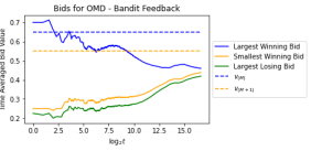
Figure 2: Time averaged bids under market dynamics for the setting described in Section 7.1. The left (resp. right) figure corresponds with the full information setting (resp. bandit setting). In this specific instance, valuations are given by $\bm{v}_{1}=[0.89,0.7,0.55,0.51,0.29],v_{2}=[0.89,0.44,0.2,0.12,0.05],v_{3}=[0.67,0.64,0.45,0.27,0.02]$.

Utilities Dynamics. In Figure 3, we analyze the time averaged utility of the agent in the market dynamics induced when all agents bid according to Algorithm 2 under the full info setting and Algorithm 4 under the bandit setting. In both the full information and bandit feedback settings, the utilities converge to the optimal utilities overtime; albeit significantly faster in the full information setting. As a consequence, the algorithms converge to a welfare optimal CCE. We also note that the hindsight optimal utility for each bidder differs across the two settings, potentially due to the different prices converged to. One interesting observation is that the shape of the regret curves are similar for both settings, indicating that the agents learned similar sets of strategies under, albeit more slowly and with higher variance in the bandit feedback setting.

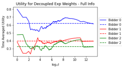
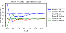
Figure 3: Time averaged utilities under market dynamics for the setting described in Section 7.1. The left (resp. right) figure corresponds with the full information setting (resp. bandit setting). In this specific instance, valuations are given by $\bm{v}_{1}=[0.89,0.7,0.55,0.51,0.29],v_{2}=[0.89,0.44,0.2,0.12,0.05],v_{3}=[0.67,0.64,0.45,0.27,0.02]$.

Distribution of Revenues. In Figure 4, we compare the distribution of per-item time averaged revenue under Algorithm  2 for the full information setting and Algorithm 4 for the bandit setting. Here, we normalize by either the per-item average welfare or by the $\overline{M}$’th and $\overline{M}+1$ largest valuations (i.e., $v_{(\overline{M})}$ and $v_{(\overline{M}+1)}$). We also plot both the time averaged and last iterate versions to see that the bids did indeed converge last-iterate wise. We note that while the revenues are generally lower in the bandit setting, the distribution of revenue of both algorithms generally maintain the same shape and it is not too heavy tailed towards low revenue. In fact, in most cases, the revenue returned is at least half of the maximum welfare. This is hopeful considering that the impact of strategizing and bid shading is large as there are a small number $N=3$ agents. We further note that revenue recovered is actually smaller than both $v_{(\overline{M})}$ and $v_{(\overline{M}+1)}$. This suggests that in some cases, there exists an agent whose valuation exceeds the clearing price, but does not actually learn to win this item; as they have foregone exploring this possibility in order to lower their payments for units they are already winning. Indeed, in several instances, some agents fail to learn their hindsight optimal bid and incur large regret.

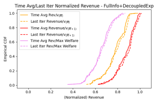
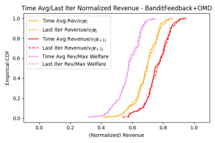
Figure 4: Distribution of revenue for the setting described in Section 7.1. The left (resp. right) figure corresponds with the full information setting (resp. bandit setting).

Welfare and Revenue Over Time. In Figure 5, we further compare the distribution of welfare and revenue over time showing the 10th, 25th, 50th, 75th, and 90th percentiles in different shades under Algorithm 2 and Algorithm 4. We normalize both welfare and revenue by the maximum possible welfare (sum of the largest $M$ valuations) in each instance. In comparison to the full information version, it takes longer for the bidders to settle to an approximately welfare maximizing steady state in the bandit setting. Furthermore, the revenue at the recovered steady state under bandit feedback is lower than that of the full information setting, albeit with lower variance.

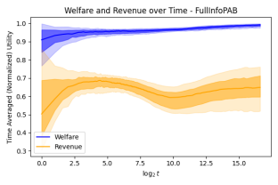
Figure 5: Welfare and revenue over time under the market dynamics for the setting described in Section 7.1. The left (resp. right) figure corresponds with the full information setting (resp. bandit setting).

.

Impact of Competition. In Figure 6, we compare the distribution of welfare and revenue over time showing the 10th, 25th, 50th, 75th, and 90th percentiles in different shades under Algorithm 4 for the bandit setting for a varying number of market participants $N\in\{12,48\}$ with $T=10^{4}$. Compared with the previous experiment with $N=3$ bidders, we see that as $N$ grows larger, there is less incentive for agents to bid strategically as there is more competition, and thus, the agents’ bids, welfare, and revenue converge more quickly. Additionally, the increased competition also improves the revenue, as expected.

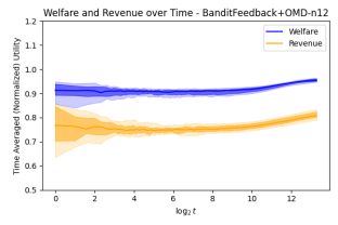
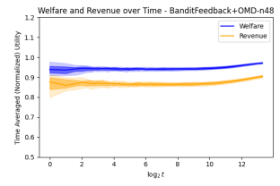
Figure 6: Effect of competition under the market dynamics for the setting described in Section 7.1. In the left figure, the number of agents is 12 while in the right one, it is 48. In both figures, we run Algorithm 4.

.

7.2 PAB vs. Uniform Price Auction Market Dynamics

In the following set of experiments, we compare the bids, welfare, and revenue of the no-regret market dynamics recovered in the uniform price auction (using the same parameterizations $N=3,M=5,|\mathcal{B}|=20,T=10^{5}$ and valuations as for the PAB learning algorithms). More specifically, we implement the no-regret learning algorithm for the uniform price auction as described in Brânzei et al. (2023), with the payment equal to the smallest winning bid. (An alternative approach would be to set the payment equal to the largest losing bid. However, as argued in Burkett and Woodward (2020), Brânzei et al. (2023), this strategy yields low revenue under Nash Equilibria. This insight has inspired us to set the payment equal to the smallest winning bid in our implementation of uniform price auctions.)

In our implementation of these algorithms, we impose no-overbidding constraint just as we had in the PAB setting, which prevents the learning dynamics from converging to a non-IR equilibrium. Similarly, we also use the EXP3-IX based estimator in the bandit uniform price algorithm to be consistent with the PAB implementation. In Sections 9.7.3 and 9.8, we run additional experiments that provide more detail regarding the regret rates, bid dynamics, and the evolution of revenue and welfare of the uniform price auction.

Time Averaged Welfare and Revenue. In Figure 7, we present a direct comparison of the time-averaged welfare and revenue (normalized by maximum welfare) between the PAB and uniform price auctions, considering both full information and bandit feedback scenarios. The plot includes the median (represented by a horizontal line), mean (indicated by an ‘x’), 25th and 75th percentiles, as well as the minimum and maximum values for welfare and revenue. Our observations reveal that in both full information and bandit feedback settings, the uniform price dynamics yield slightly higher welfare but significantly lower revenue compared to the PAB dynamics. This disparity is further amplified in the bandit feedback scenario. Specifically, in bandit feedback, the mean welfare for the uniform price auction is 0.980 (with a standard deviation of 0.028), while the PAB mechanism achieves a mean welfare of 0.952 (with a standard deviation of 0.049). Similarly, the mean revenue for the uniform price auction is 0.481 (with a standard deviation of 0.194), whereas the PAB mechanism achieves a mean revenue of 0.626 (with a standard deviation of 0.091). It is worth noting that the variance in uniform price revenue under bandit feedback is particularly concerning, as the revenue can be as low as 8% of the maximum welfare, compared to 39% under the PAB mechanism. Conversely, the minimum welfare achieved under bandit feedback for the PAB mechanism is 77%, while the uniform price auction attains a minimum welfare of 86%.

The slight decrease in welfare observed in PAB can be attributed to the increased incentive for bidders to understate their bids in order to reduce their payment. In PAB, the payment and utility for each individual unit directly depend on the bid placed on that specific unit. On the other hand, in the uniform price auction, the payment is determined by the lowest winning bid, and there is consequently less motivation to manipulate higher bids since they are less correlated with the payment. This observation aligns with findings from other variants of discriminatory versus uniform pricing, such as generalized first and second price auctions. Conversely, the improved stability and higher revenue observed in PAB can be attributed to the ability of bidders to strategically shade their bids on a per-unit basis. In PAB, bidders have more direct control over their payments compared to the uniform price auction, where the payment per unit can fluctuate significantly depending on a single clearing price. This increased control allows bidders to optimize their bids strategically and leads to enhanced stability and higher revenue in the PAB mechanism.

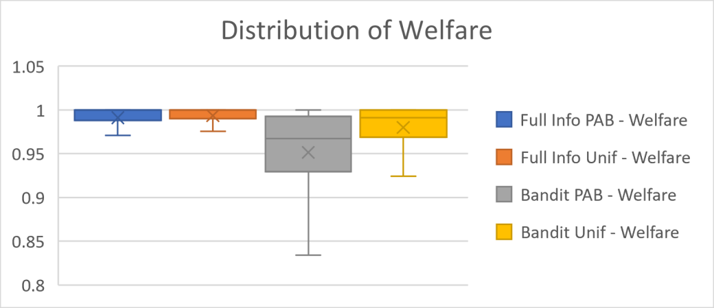
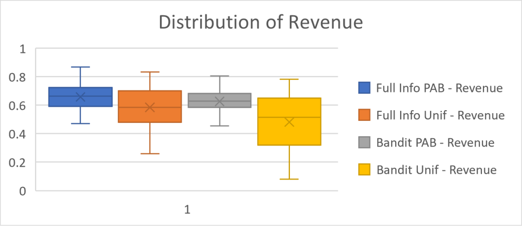
Figure 7: Welfare (left) and revenue (right) comparisons between the PAB and Uniform Price auctions, under both full information and bandit feedback. We use the setting described in Section 7.2.

Convergence of Bids. In Figure 8, we compare the ratios of (i) the largest to the smallest winning bid and (ii) the smallest winning bid to the largest losing bid. We plot these ratios over time for both the PAB and uniform price auctions, under bandit feedback only (we exclude full information feedback as the differences in welfare and revenue are negligible). We make the crucial observation that while both ratios converge to 1 ($\log_{2}1=0$ in the plot) in the PAB auction, the ratio of the largest to smallest winning bid in the uniform price auction does not converge to 1. The convergence of these ratios for the PAB setting indicate that the optimal bidding strategy for the PAB auction is uniform bidding. In contrast, the non-convergence for the uniform price setting suggests that the optimal bidding in the uniform price auction requires discriminatory bidding (different prices for each unit). See our discussions in Section 1.2 regarding the practical implications of this observation.

Furthermore, we observe that the ratio of the smallest winning to largest losing bids converges noticeably more slowly under the uniform price auction. This slower convergence can be attributed to the increased number of edge weights $O(M|\mathcal{B}|^{2})$ required to learn in the uniform price auction as compared to the $O(M|\mathcal{B}|)$ node weights in the PAB auction.

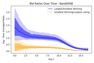
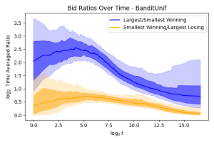
Figure 8: We compare the ratios of the largest winning bid to the smallest winning bid and also the smallest winning bid to the largest losing bid for the setting described in Section  7.1. The left (resp. right) figure corresponds with the PAB dynamics (Uniform pricing dynamics).

.

8 Concluding Remarks

We have provided low-regret learning algorithms for PAB auctions in the full information and bandit settings with corresponding polynomial time and space complexities. In particular, we utilize our DP formulation and its equivalent graph representation to decouple the utility associated with bidding $b_{m}=b$ for all $m\in[M],b\in\mathcal{B}$. We derived two algorithms, one that mimics the exponential weights algorithm and another based on OMD, both of which allowed us to achieve polynomial (in $M$, $|\mathcal{B}|$, and $T$) regret upper bounds, as well as time and space complexities, despite the combinatorially large bid space.

There are several intriguing avenues for future research that can be explored based on the current work. A promising direction is to leverage the structure induced by bid monotonicity in PAB auctions. Recent advancements in a simpler single-unit setting have demonstrated the efficacy of cross-learning between bids under certain feedback structures (Han et al. 2020a, Han et al. 2020b). It would be intriguing to investigate the potential benefits of applying cross-learning techniques in our multi-unit setting. By incorporating such methods, we can explore whether they can enhance our regret bounds. Furthermore, inspired by our numerical results—where we show that the winning bids in PAB market dynamics converge to the same value—we can explore the design of online learning algorithms for the setting where bidders are restricted to a simplified bidding interface, wherein they are only allowed to submit a single price and quantity for the units demanded rather than an entire vector of bids.

9 Appendix

9.1 Proof of Theorem 3.1: Offline Bid Optimization Algorithm

We give a proof of correctness of the offline bid optimization algorithm used to compute the hindsight optimal bid vector across $T$ rounds of PAB auctions. Our proof shows that the variables $U_{m}(b)$ are path weights of the optimal partial bid vector with weights $W_{m}^{T+1}(b)$. Thus, $U_{1}(b)$ is the optimal bid vector and $b^{*}_{m}$’s can be used to back out the optimal bid vector recursively in polynomial time.

Proof 9.1

Proof of Theorem 3.1 By definition,

$$U_{m}(b) =\max_{b\geq b_{m}\geq\ldots\geq b_{M}}\sum_{m^{\prime}=m}^{M}W^{T+1}_{m^{\prime}}(b_{m^{\prime}})$$

$$=\max_{b\geq b_{m}\geq\ldots\geq b_{M}}W^{T+1}_{m}(b_{m})+\sum_{m^{\prime}=m+1}^{M}W^{T+1}_{m^{\prime}}(b_{m^{\prime}})$$

$$=\max_{b^{\prime}\leq b}W^{T+1}_{m}(b^{\prime})+U_{m+1}(b^{\prime})\,.$$

Since we have that $U_{M}(b)=W^{T+1}_{M}(b)$ trivially correct from the base case, and the optimality of $U_{m}(b)$ follows from induction. Consequently, optimality of $b_{m}^{*}$ follows from induction. The base case trivially holds as $b_{1}^{*}=\text{argmax}_{b\in\mathcal{B}}U_{1}(b)$. The recursive case also follows straightforwardly by definition of $b^{*}_{m}$:

$$b^{*}_{m}=\text{argmax}_{b\leq b^{*}_{m-1}}U_{m}(b)\,.$$

As $b^{*}_{m-1}$ was optimal by the induction hypothesis, then $b_{m}^{*}$ must also be optimal.

We finish this proof by discussing the time and space complexity of Algorithm 1. Table $U$ is of size $O(M|\mathcal{B}|)$, with each entry requiring taking a maximum over $O(|\mathcal{B}|)$ terms, yielding time and space complexities of $O(M|\mathcal{B}|^{2})$ and $O(M|\mathcal{B}|)$ respectively.

9.2 Proof of Theorems 4.1 and 4.2: Decoupled Exponential Weights Algorithm

Proof 9.2

We give the proofs of correctness, complexity analysis, and regret analysis for the decoupled exponential weights algorithms for both the full information (Algorithm 2) and the bandit setting (Algorithm 3). Our proof comes in 5 parts. We first prove correctness of the bandit version of our algorithm. In particular, we show that defining the node and bid vector utility estimates to be $\widehat{w}_{m}^{t}(b)=1-\frac{1-(v_{m}-b)1_{b\geq b_{-m}^{t}}}{q_{m}^{t}(b)}1_{b=b^{t}_{m}}$ and $\widehat{\mu}^{t}(\bm{b})=\sum_{m=1}^{M}\widehat{w}_{m}^{t}(b_{m})$, our algorithm samples bid vector $\bm{b}^{t}$ with probability proportional to $\exp(\eta\sum_{\tau=1}^{t-1}\widehat{\mu}^{\tau}(\bm{b}))$ via the same recursive sampling procedure as in Algorithm 2. In the second part and third parts, we derive a corresponding regret upper bound and obtain the time and space complexities of our algorithm with bandit feedback. In the fourth part, we optimize the continuous regret w.r.t. the selection of $\mathcal{B}$. In the fifth part, we show how to extend our algorithm and results to the full information setting.

Part 1: Algorithm Correctness. In this part of the proof, we argue that our choice of estimator is unbiased and that Algorithm 3 samples bid vectors with the same probability that the exponential weights algorithm would have, given the same node utility estimates $\widehat{w}_{m}^{t}(b)$. To show unbiasedness of $\widehat{w}_{m}^{t}(b)$, we have:

$$\mathbb{E}\left[\widehat{w}_{m}^{t}(b)\right]=\mathbb{E}\left[1-\frac{1-w^{t}_{m}(b)}{q^{t}_{m}(b)}\textbf{1}_{b^{t}_{m}=b}\right]=\mathbb{E}\left[1-\frac{\textbf{1}_{b^{t}_{m}=b}}{q^{t}_{m}(b)}+\frac{\textbf{1}_{b^{t}_{m}=b}\cdot w^{t}_{m}(b)}{q^{t}_{m}(b)}\right]=w^{t}_{m}(b)\,.$$

Now, it remains to show that our sampling procedure $\textsc{Sample}-\bm{b}$ w.r.t. $\widehat{S}^{t}_{m}$ indeed samples bid vectors $\bm{b}$ with the same probability as the exponential weights algorithm under weights $\widehat{\mu}^{t}_{n}(\bm{b})$. In particular, we want to show that our algorithm samples bid vectors $\bm{b}^{t}$ with probability proportional to $\exp(\eta\sum_{\tau=1}^{t-1}\widehat{\mu}_{m}^{\tau}(b_{m}))$ for any $m\in[M]$. This follows from analyzing the dynamic programming variables that represent the sum of exponentiated (estimated) partial bid vector utilities, $\widehat{S}$.

In exponential weights, the bidder selects at round $t+1$ some action $\bm{b}$ with probability $P^{t}(\bm{b})$ proportional to $\sum_{\tau=1}^{t}\widehat{\mu}_{n}^{t}(b)$. Using our representation of $\widehat{\mu}_{n}^{t}(\bm{b})$ as a function $\widehat{w}_{m}^{\tau}(b)$, we have:

$$P^{t}(\bm{b})=\frac{\exp(\eta\sum_{\tau=1}^{t-1}\widehat{\mu}_{n}^{\tau}(\bm{b}))}{\sum_{\bm{b}^{\prime}\in\mathcal{B}^{+M}}\exp(\eta\sum_{\tau=1}^{t-1}\widehat{\mu}_{n}^{\tau}(\bm{b}^{\prime}))}=\frac{\exp(\eta\sum_{m=1}^{M}\widehat{W}_{m}^{t}(b_{m}))}{\sum_{\bm{b}^{\prime}\in\mathcal{B}^{+M}}\exp(\eta\sum_{m=1}^{M}\widehat{W}_{m}^{t}(b^{\prime}_{m}))}\,.$$

Hence, we wish to construct a sampler that samples $\bm{b}$ with the above probability. Defining $b_{0}=\max_{b\in\mathcal{B}}b$, we begin by decomposing the denominator as follows:

$$\sum_{\bm{b}\in\mathcal{B}^{+M}}\exp(\eta\sum_{m=1}^{M}\widehat{W}_{m}^{t}(b_{m}))=\sum_{b_{1}\in\mathcal{B},b_{1}\leq b_{0}}\sum_{b_{2}\in\mathcal{B},b_{2}\leq b_{1}}\ldots\sum_{b_{M}\in\mathcal{B},b_{M}\leq b_{M-1}}\exp(\eta\sum_{m=1}^{M}\widehat{W}_{m}^{t}(b_{m}))$$

$$=\sum_{b_{1}\in\mathcal{B},b_{1}\leq b_{0}}\exp(\eta\widehat{W}_{1}^{t}(b_{1}))\sum_{b_{2}\in\mathcal{B},b_{2}\leq b_{1}}\exp(\eta\widehat{W}_{2}^{t}(b_{2}))\ldots\sum_{b_{M}\in\mathcal{B},b_{M}\leq b_{M-1}}\exp(\eta\widehat{W}_{M}^{t}(b_{M}))\,.$$

Recall a key object $\widehat{S}^{t}_{m}(b)$, which is the sum of exponentially weighted utilities of partial bid vectors $\bm{b}^{\prime}_{m:M}\in\mathcal{B}^{+(M-m+1)}$ over slots $m,\ldots,M$ subject to $b_{m}=b$.

$$\widehat{S}^{t}_{m}(b) =\exp(\eta\widehat{W}_{m}^{t}(b))\sum_{\bm{b}^{\prime}_{m+1:M}\in\mathcal{B}^{+(M-m)},b^{\prime}_{m+1}\leq b^{\prime}_{m}=b}\exp(\eta\sum_{m^{\prime}=m+1}^{M}\widehat{W}_{m^{\prime}}^{t}(b^{\prime}_{m^{\prime}}))$$ (8)

$$=\exp(\eta\widehat{W}_{m}^{t}(b))\sum_{b^{\prime}\in\mathcal{B};b^{\prime}\leq b}\widehat{S}^{t}_{m+1}(b^{\prime})\,.$$ (9)

With the trivial base case $\widehat{S}^{t}_{M}(b)=\exp(\eta\widehat{W}_{M}^{t}(b))$, we can recover all of the exponentially weighted partial utilities $\{\widehat{S}^{t}_{m}(b)\}_{m\in[M],b\in\mathcal{B}}$ given $\bm{W}^{t}$. Once we have computed $\{\widehat{S}^{t}_{m}(b)\}_{m\in[M],b\in\mathcal{B}}$, we can sample $\bm{b}$ according to its exponentially weighted utility $\exp(\eta\widehat{\mu}^{t}_{m}(\bm{b}))$ by sequentially sampling each $b_{1},\ldots,b_{M}$.

Let $P_{\textsc{D}}^{t}(\bm{b})$ be the probability that our Algorithm 3 returns bid vector $\bm{b}\in\mathcal{B}^{+M}$ in round $t$. Recall that we sample $\bm{b}$ by setting $b_{m}^{t}$ to $b\in\mathcal{B},b\leq b_{m-1}^{t}$ with probability $\frac{\widehat{S}^{t}_{m}(b)}{\sum_{b^{\prime}\leq b_{m-1}^{t}}\widehat{S}^{t}_{m}(b^{\prime})}$. Hence, the probability of selecting $\bm{b}$ is the product of $m$ conditional probability mass functions (pmf’s) and we have

$$P_{\textsc{D}}^{t}(\bm{b})=\prod_{m=1}^{M}\frac{\widehat{S}^{t}_{m}(b_{m})}{\sum_{b^{\prime}\leq b_{m-1}}\widehat{S}^{t}_{m}(b^{\prime})}=\left(\prod_{m=1}^{M-1}\frac{\exp(\eta\widehat{W}_{m}^{t}(b_{m}))\sum_{b\leq b_{m}}\widehat{S}^{t}_{m+1}(b)}{\sum_{b^{\prime}\leq b_{m-1}}\widehat{S}^{t}_{m}(b^{\prime})}\right)\left(\frac{\exp(\eta\widehat{W}_{M}^{t}(b_{M}))}{\sum_{b^{\prime}\leq b_{M-1}}\widehat{S}_{M}^{t}(b^{\prime})}\right)\,.$$

Moving the $\exp(\eta\widehat{W}_{m}^{t}(b_{m}))$ outside of the product, we obtain:

$$P_{\textsc{D}}^{t}(\bm{b}) =\left(\prod_{m=1}^{M-1}\exp(\eta\widehat{W}_{m}^{t}(b_{m}))\right)\left(\prod_{m=1}^{M-1}\frac{\sum_{b\leq b_{m}}\widehat{S}^{t}_{m+1}(b)}{\sum_{b^{\prime}\leq b_{m-1}}\widehat{S}^{t}_{m}(b^{\prime})}\right)\left(\frac{\exp(\eta\widehat{W}_{M}^{t}(b_{M}))}{\sum_{b^{\prime}\leq b_{M-1}}\widehat{S}_{M}^{t}(b^{\prime})}\right)$$

$$=\left(\prod_{m=1}^{M}\exp(\eta\widehat{W}_{m}^{t}(b_{m}))\right)\left(\frac{\sum_{b\leq b_{M-1}}\widehat{S}^{t}_{M}(b)}{\sum_{b^{\prime}\leq b_{0}}\widehat{S}^{t}_{1}(b^{\prime})}\right)\left(\frac{1}{\sum_{b^{\prime}\leq b_{M-1}}\widehat{S}_{M}^{t}(b^{\prime})}\right)$$

$$=\frac{\prod_{m=1}^{M}\exp(\eta\widehat{W}_{m}^{t}(b_{m}))}{\sum_{b^{\prime}\leq b_{0}}\widehat{S}_{1}^{t}(b^{\prime})}\,.$$

We now rearrange the last expression to see that our algorithm samples $\bm{b}$ with the same probability as the exponential weights algorithm:

$$P_{\textsc{D}}^{t}(\bm{b})=\frac{\prod_{m=1}^{M}\exp(\eta\widehat{W}_{m}^{t}(b_{m}))}{\sum_{b\leq b_{0}}S_{1}^{t}(b)}=\frac{\exp(\eta\sum_{m=1}^{M}\widehat{W}_{m}^{t}(b_{m}))}{\sum_{\bm{b}^{\prime}\in\mathcal{B}^{+M}}\exp(\eta\sum_{m=1}^{M}\widehat{W}_{m}^{t}(b^{\prime}_{m}))}=P^{t}(\bm{b})\,.$$

Part 2: Regret Analysis. We are now ready to derive the regret upper bound on Algorithm 3. First, we show that the bid vector utility estimators $\widehat{\mu}^{t}(\bm{b})$ are both unbiased and have a finite upper bound. To show the upper bound, we take expectation with respect to the bid vectors selected by our algorithm and observe that

$$\mathbb{E}[\widehat{\mu}^{t}(\bm{b})] =\sum_{m=1}^{M}\mathbb{E}[\widehat{w}_{m}^{t}(b_{m})]=\sum_{m=1}^{M}\mathbb{E}\left[1-\frac{1-(v_{m}-b_{m})1_{b_{m}>b_{-m}^{t}}}{q_{m}^{t}(b_{m})}1_{b_{m}=b^{t}_{m}}\right]$$

As we are considering the expectation ex-post, keeping the $b_{-m}^{t}$’s fixed, we have independence between the two indicator functions and we obtain:

$$=\sum_{m=1}^{M}\mathbb{E}\left[1-\frac{1-w^{t}_{m}(b_{m})}{q_{m}^{t}(b_{m})}1_{b_{m}=b^{t}_{m}}\right]=M-\sum_{m=1}^{M}\frac{1-w^{t}_{m}(b_{m})}{q_{m}^{t}(b_{m})}\mathbb{E}\left[1_{b_{m}=b^{t}_{m}}\right]=\mu^{t}(\bm{b})\,.$$

As for the finite upper bound, we have that $\widehat{\mu}^{t}(\bm{b})=\sum_{m=1}^{M}\widehat{w}_{m}^{t}(b_{m})$ is the sum over $M$ node utility estimators, each of which is upper bounded by 1. Hence, $\widehat{\mu}^{t}(\bm{b})\leq M$ for all $\bm{b}\in\mathcal{B}^{+M}$. Now, we make the following claim:

Lemma 9.3

Let $\widehat{\mu}^{t}(\bm{b})=\sum_{m=1}^{M}(1-\frac{1-(v_{m}-b_{m})1_{b_{m}>b_{-m}^{t}}}{q_{m}^{t}(b_{m})}1_{b_{m}=b^{t}_{m}})$ be our bid vector utility estimate as discussed. Then, any algorithm which samples bid vectors $\bm{b}$ with probability proportional to $\exp(\eta\sum_{\tau=1}^{t-1}\widehat{\mu}^{t}(\bm{b}))$ at round $t$ for $\eta\leq\frac{1}{M}$ has regret upper bound

$$\textsc{Regret}_{\mathcal{B}}\lesssim\eta^{-1}M\log|\mathcal{B}|+\eta\sum_{t=1}^{T}\sum_{\bm{b}}$$ (10)

Proof 9.4

Proof of Lemma 9.3 We will closely follow the analysis of the Exp3 algorithm as presented in Chapter 11.4 of Lattimore and Szepesvári (2020). In particular, we follow their regret analysis until Equation 11.13. Define $\Phi^{t}=\sum_{\bm{b}\in\mathcal{B}^{+M}}\exp(\eta\sum_{\tau=1}^{t}\widehat{\mu}^{\tau}(\bm{b}))$ to be the potential at round $t$. As per our initial conditions in Algorithm 3, we have $\widehat{\mu}^{0}(\bm{b})=0$, and consequently, $\Phi^{0}=|\mathcal{B}^{+M}|$. While it is not immediately apparent how the potentials $\Phi^{t}$ relate to the regret, we begin by upper bounding $\exp(\eta\sum_{t=1}^{T}\widehat{\mu}^{t}(\bm{b}))$ for a fixed $\bm{b}^{\prime}$:

$$\exp(\eta\sum_{t=1}^{T}\widehat{\mu}^{t}(\bm{b}^{\prime}))\leq\sum_{\bm{b}\in\mathcal{B}^{+M}}\exp(\eta\sum_{t=1}^{T}\widehat{\mu}^{t}(\bm{b}))=\Phi^{T}=\Phi^{0}\prod_{t=1}^{T}\frac{\Phi^{t}}{\Phi^{t-1}}\,.$$ (11)

Now, we upper bound each $\frac{\Phi^{t}}{\Phi^{t-1}}$:

$$\frac{\Phi^{t}}{\Phi^{t-1}}=\sum_{\bm{b}\in\mathcal{B}^{+M}}\frac{\exp(\eta\sum_{\tau=1}^{t}\widehat{\mu}^{\tau}(\bm{b}))}{\Phi^{t-1}}=\sum_{\bm{b}\in\mathcal{B}^{+M}}\frac{\exp(\eta\sum_{\tau=1}^{t-1}\widehat{\mu}^{\tau}(\bm{b}))}{\Phi^{t-1}}\exp(\eta\widehat{\mu}^{t}(\bm{b}))=\sum_{\bm{b}\in\mathcal{B}^{+M}}$$

where in the last equality, we used the condition that our algorithm samples bid vector $\bm{b}$ with probability proportional to $\exp(\eta\sum_{\tau=1}^{t-1}\widehat{\mu}^{t}(\bm{b}))$ at round $t$. In order to continue the chain of inequalities, we note that for $\eta\leq\frac{1}{M}$, we have that the quantity $\eta\widehat{\mu}^{t}(\bm{b})$ is upper bounded by 1 as $\eta\widehat{\mu}^{t}(\bm{b})\leq\eta M\leq 1$. In the first inequality, we used the fact that $\widehat{\mu}^{t}(\bm{b})\leq M$. Now, we can apply the inequalities $\exp(x)\leq 1+x+x^{2}$ and $1+x\leq\exp(x)$ for all $x\leq 1$, with $x=\eta\widehat{\mu}^{t}(\bm{b})$ and $x=\eta$, respectively, to obtain:

$$\frac{\Phi^{t}}{\Phi^{t-1}} \leq\sum_{\bm{b}\in\mathcal{B}^{+M}}$$

$$\leq\sum_{\bm{b}\in\mathcal{B}^{+M}}$$

$$=1+\sum_{\bm{b}\in\mathcal{B}^{+M}}$$

$$\leq\exp(\sum_{\bm{b}\in\mathcal{B}^{+M}}$$

Combining this with Equation (11) and then taking logarithms, we obtain:

$$\eta\sum_{t=1}^{T}\widehat{\mu}^{t}(\bm{b}^{\prime})\leq\log\Phi^{0}+\eta\sum_{t=1}^{T}\sum_{\bm{b}\in\mathcal{B}^{+M}}$$

Dividing both sides by $\eta$, applying the upper bound on $\Phi^{0}$, and rearranging, we obtain that for any $\bm{b}^{\prime}\in\mathcal{B}^{+M}$:

$$\sum_{t=1}^{T}\widehat{\mu}^{t}(\bm{b}^{\prime})-\sum_{t=1}^{T}\sum_{\bm{b}\in\mathcal{B}^{+M}}$$

Replacing $\widehat{\mu}^{t}(\bm{b})$ with its definition in terms of $\widehat{w}^{t}_{m}(b_{m})$ and taking expectations, we obtain the right hand side of the lemma:

$$\mathbb{E}\left[\sum_{t=1}^{T}\widehat{\mu}^{t}(\bm{b}^{\prime})-\sum_{t=1}^{T}\sum_{\bm{b}\in\mathcal{B}^{+M}}\right]\lesssim\eta^{-1}M\log|\mathcal{B}|+\eta\sum_{t=1}^{T}\sum_{\bm{b}}$$

Replacing $\sum_{\bm{b}\in\mathcal{B}^{+M}}$ with $\mathbb{E}[\widehat{\mu}^{t}(\bm{b}^{t})]$ and recalling that the bid vector utility estimates $\widehat{\mu}^{t}$ were unbiased, we have:

$$\sum_{t=1}^{T}\mu^{t}(\bm{b}^{\prime})-\sum_{t=1}^{T}\mathbb{E}[\mu^{t}(\bm{b}^{t})]\lesssim\eta^{-1}M\log|\mathcal{B}|+\eta\sum_{t=1}^{T}\sum_{\bm{b}}$$

Notice that as this is true for any $\bm{b}^{\prime}$, we can replace it with the bid vector that maximizes the true cumulative utility $\sum_{t=1}^{T}\mu^{t}(\bm{b}^{\prime})$ and see that the left hand side becomes precisely $\textsc{Regret}_{\mathcal{B}}$, which completes the proof.

Now, it remains to show an upper bound on the second moment of the bid vector utility estimate $\mathbb{E}[(\sum_{m=1}^{M}\widehat{w}^{t}_{m}(b_{m}))^{2}]$. A crude attempt would be to say that $\mathbb{E}[(\sum_{m=1}^{M}\widehat{w}^{t}_{m}(b_{m}))^{2}]\leq M\sum_{m=1}^{M}\mathbb{E}[\widehat{w}^{t}_{m}(b_{m})^{2}]$:

$$\sum_{t=1}^{T}\sum_{\bm{b}}$$ (12)

$$=M\sum_{t=1}^{T}\sum_{m=1}^{M}\sum_{b\in\mathcal{B}}\mathbb{E}[\widehat{w}^{t}_{m}(b)^{2}]\sum_{\bm{b}:b_{m}=b}$$

$$\leq M\sum_{t=1}^{T}\sum_{m=1}^{M}\sum_{b\in\mathcal{B}}\frac{2}{q_{m}^{t}(b)}q_{m}^{t}(b)=O(M^{2}|\mathcal{B}|T)\,.$$

Where the last inequality follows from:

$$\mathbb{E}[\widehat{w}_{m}^{t}(b)^{2}]=\mathbb{E}\left[\left(1-\frac{1-w_{m}^{t}(b)}{q_{m}^{t}(b)}\textbf{1}_{b_{m}^{t}=b}\right)^{2}\right]=1-2\mathbb{E}\left[\frac{1-w_{m}^{t}(b)}{q_{m}^{t}(b)}\textbf{1}_{b_{m}^{t}=b}\right]+\mathbb{E}\left[\left(\frac{1-w_{m}^{t}(b;\bm{v})}{q_{m}^{t}(b)}\right)^{2}\textbf{1}_{b_{m}^{t}=b}\right]\,.$$

Evaluating the expectations with $\mathbb{E}\left[\textbf{1}_{b_{m}^{t}=b}\right]=q_{m}^{t}(b)$, we have:

$$\mathbb{E}[\widehat{w}_{m}^{t}(b)^{2}]=1-\left[2-2w_{m}^{t}(b)\right]+\left[\frac{(1-w_{m}^{t}(b))^{2}}{q_{m}^{t}(b)}\right]=2w_{m}^{t}(b)-1+\frac{1}{q_{m}^{t}(b)}\leq 1+\frac{1}{q_{m}^{t}(b)}\leq\frac{2}{q_{m}^{t}(b)}\,.$$

Plugging this back into our upper bound yields stated regret bound for $\eta=\Theta(\sqrt{\frac{\log|\mathcal{B}|}{M|\mathcal{B}|T}})$ such that $\eta<\frac{1}{M}$:

$$\textsc{Regret}_{\mathcal{B}}\lesssim\eta^{-1}M\log|\mathcal{B}|+\eta M^{2}|\mathcal{B}|T=O(M^{\frac{3}{2}}\sqrt{|\mathcal{B}|T\log|\mathcal{B}|})\,.$$

Part 3: Complexity Analysis. We note that the time and space complexity analysis is identical to that of Algorithm 2, as the only additional computational work being done is computing the normalization terms $q_{m}^{t}(b)$, which requires $O(M|\mathcal{B}|)$ space and $O(MT|\mathcal{B}|)$ time respectively. Hence, discarding old tables, the total time and space complexities of Algorithm 3 are $O(M|\mathcal{B}|T)$ and $O(M|\mathcal{B}|)$ respectively. As this is polynomial in $M,|\mathcal{B}|,T$, we have proven the claim of polynomial space and time complexities.

Part 4: Selecting $\mathcal{B}$. We claim that the sub-optimality due to the discretization is on the order of $\frac{MT}{|\mathcal{B}|}$. Assume that $\mathcal{B}\equiv\{\frac{i}{|\mathcal{B}|}\}_{i\in[|\mathcal{B}|]}$ is an even discretization of $[0,1]$., and recall the continuous regret benchmark:

$$\textsc{Regret}=\max_{\bm{b}\in[0,1]^{+M}}\sum_{t=1}^{T}\mu^{t}_{n}(\bm{b})-\mathbb{E}\left[\sum_{t=1}^{T}\mu^{t}_{n}(\bm{b}^{t})\right],$$

where the maximum is taken over the entire space $[0,1]^{+M}$ rather than $\mathcal{B}^{+M}$. Let $\bm{b}^{*}$ denote the maximizer of the continuous regret. Then, bidder $n$ could have obtained at least the same allocation by rounding up each bid in $\bm{b}^{*}$ to the next largest multiple of $\frac{1}{|\mathcal{B}|}$. Let this rounded bid vector be denoted by $\bm{b}^{+}$. As their allocation, thus value for the set of items received, does not decrease, and their total payment increases by a maximum of $\frac{M}{|\mathcal{B}|}$ at each round, then we have that $\mu_{n}^{t}(\bm{b}^{+})\geq\mu_{n}^{t}(\bm{b}^{*})-\frac{M}{|\mathcal{B}|}$. Let $\bm{b}_{\mathcal{B}}^{*}\in\mathcal{B}^{+M}$ denote the hindsight optimal utility vector returned by our offline dynamic programming (Algorithm 1), which serves as the regret benchmark in the definition of discretized regret. Noting that $\bm{b}^{+}\in\mathcal{B}^{+M}$, we have that the total utility of bidding $\bm{b}^{*}_{\mathcal{B}}$ must be at least that of $\bm{b}^{+}$. Thus,

$$\sum_{t=1}^{T}\mu^{t}_{n}(\bm{b}_{\mathcal{B}}^{*})\geq\sum_{t=1}^{T}\mu^{t}_{n}(\bm{b}^{+})\geq\sum_{t=1}^{T}\mu^{t}_{n}(\bm{b}^{*})-\frac{MT}{|\mathcal{B}|}$$

We balance this with the discretized regret $O(M^{\frac{3}{2}}\sqrt{|\mathcal{B}|T\log|\mathcal{B}|})$ with $|\mathcal{B}|=M^{-\frac{1}{3}}T^{\frac{1}{3}}$. This yields continuous regret $\textsc{Regret}=O(M^{\frac{4}{3}}T^{\frac{2}{3}}\sqrt{\log T})$.

Part 5: Extending to the Full Information Setting. Thus far, we have only discussed the bandit feedback algorithm. Fortunately, the full information setting algorithm is exactly the same except for two differences: 1) we do not need to compute $\bm{q}$ and 2) we can replace the reward estimates $\widehat{\mu}^{t}(\bm{b})$ with the true rewards $\mu^{t}(\bm{b})$ in Equation LABEL:eq:_full_info_difference. The first difference can only serve to improve the time and space complexity of our algorithm. The second difference allows us to improve the bound on $\sum_{t=1}^{T}\sum_{\bm{b}}$ in the left hand sight of Equation LABEL:eq:_full_info_difference by replacing $\widehat{w}^{t}_{m}(b_{m}))$ with $w^{t}_{m}(b_{m})$:

$$\sum_{t=1}^{T}\sum_{\bm{b}}$$

Notice that this bound is a factor of $|\mathcal{B}|$ improvement over that in the bandit setting. Consequently, we obtain our stated regret bound of $O(M^{\frac{3}{2}}\sqrt{T\log|\mathcal{B}|})$ with the choice of $\eta=\Theta(\sqrt{\frac{\log|\mathcal{B}|}{MT}})$. Balancing this regret with the error term, which is of order $O\left(\frac{M|\mathcal{B}|}{T}\right)$, the optimal choice of $|\mathcal{B}|$ is given by $\Theta(\sqrt{\frac{T}{M}})$. This yields corresponding continuous regret of $O(M^{\frac{3}{2}}\sqrt{T\log T})$.

9.3 Proof of Lemma 5.1

Proof 9.5

Proof of Lemma 5.1 In order to show equivalence, we show that (1) for any $\pi\in\Pi$, that $q(\pi)\in\mathcal{Q}$ and (2) for any $\bm{q}\in\mathcal{Q}$, there exists a $\pi\in\Pi$ such that $q(\pi)=\bm{q}$. We first prove (1). To do this, we simply need to check that for a given $\pi\in\Pi$, that $q^{\pi}=q(\pi)$ satisfies the constraints prescribed by $\mathcal{Q}$.

The non-negativity constraint holds trivially as each $\pi((m,b),b^{\prime})$ is non-negative. Since all $q^{\pi}_{1}(b)=\pi((0,\max\mathcal{B}),b)\geq 0$ for all $b\in\mathcal{B}$, by induction, $q^{\pi}_{m+1}(b)=\sum_{b"\geq b}q^{\pi}_{m}(b")\pi((m,b"),b)$ is also non-negative.

Now we prove that each layer $m$ sums to 1, i.e., $\sum_{b\in\mathcal{B}}q^{\pi}_{m}(b)=1$. Since $\sum_{b\in\mathcal{B}}q^{\pi}_{1}(b)$, the policy has total node probability 1 in the first layer, we can prove $\sum_{b\in\mathcal{B}}q^{\pi}_{m}(b)=1$, that the policy has total node probability 1 in the $m$’th layer, via induction. This follows immediately from the fact that the DP graph is layered, i.e., edges exist only from nodes in layer $m$ to nodes in layer $m+1$, thus the only edges leading to layer $m+1$ are from layer $m$, in which there are no other edges. Hence, the total node probability in layer $m+1$ must be exactly that of layer $m$. More formally, we have:

$$\sum_{b\in\mathcal{B}}q^{\pi}_{m+1}(b)=\sum_{b\in\mathcal{B}}\sum_{b"\geq b}q^{\pi}_{m}(b")\pi((m,b"),b)=\sum_{b"\in\mathcal{B}}q^{\pi}_{m}(b")\sum_{b\leq b"}\pi((m,b"),b)=\sum_{b"\in\mathcal{B}}q^{\pi}_{m}(b")\,.$$

To show the stochastic domination constraint $\sum_{b\leq b^{\prime}}q^{\pi}_{m+1}(b)\geq\sum_{b\leq b^{\prime}}q^{\pi}_{m}(b)$, we use the bid monotonicity constraint; i.e., the fact that the edges between layers are only from larger bids to (weakly) smaller bids. Recall that $\pi((m,b^{\prime}),b")$ is the probability of transitioning from unit-bid value pair $(m,b^{\prime})$ to $(m+1,b")$ and that the only edges leading to $(m+1,b")$ come from nodes $(m,b^{\prime})$ for $b^{\prime}\geq b"$. Then, we have:

$$\sum_{b\leq b^{\prime}}q^{\pi}_{m+1}(b) =\sum_{b\leq b^{\prime}}\sum_{b"\geq b}q^{\pi}_{m}(b")\pi((m,b"),b)$$

$$=\sum_{b">b^{\prime}}q^{\pi}_{m}(b")\sum_{b\leq b^{\prime}}\pi((m,b"),b)+\sum_{b"\leq b^{\prime}}q^{\pi}_{m}(b")\sum_{b\leq b"}\pi((m,b"),b)$$

$$=\sum_{b">b^{\prime}}q^{\pi}_{m}(b")\sum_{b\leq b^{\prime}}\pi((m,b"),b)+\sum_{b\leq b^{\prime}}q^{\pi}_{m}(b)$$

$$\geq\sum_{b\leq b^{\prime}}q^{\pi}_{m}(b)\,.$$

Hence, we have shown that for any $\pi\in\Pi$, that the corresponding $q(\pi)\in\mathcal{Q}$.

Now we show the other direction (2), that for any $\bm{q}\in\mathcal{Q}$, there exists a $\pi\in\Pi$ such that $q(\pi)=\bm{q}$. We proceed by showing that for all $m,b^{*}$, there exists $\{\pi((m,b),b^{\prime})\}_{b,b^{\prime}\in\mathcal{B}}$ such that the following conditions hold:

1. $\pi((m,b),b^{\prime})\geq 0$ for all $b,b^{\prime}\geq b^{*}$.

2. $\pi((m,b),b^{\prime})=0$ for all $b^{\prime}>b\geq b^{*}$.

3. $\sum_{b^{\prime}\leq b,b^{\prime}\geq b^{*}}\pi((m,b),b^{\prime})\leq 1$ for all $b^{*}\in\mathcal{B}$, with equality if and only if $b^{*}=b_{\min}$ where $b_{\min}=\min\mathcal{B}$.

4. $\sum_{b^{\prime}\geq b^{*}}\sum_{b\geq b^{\prime}}q_{m}(b)\pi((m,b),b^{\prime})=\sum_{b^{\prime}\geq b^{*}}q_{m+1}(b^{\prime})$.

Let $\Pi(b^{*};\mathbf{q})$, $b^{*}\in\mathcal{B}$, be the set of all policies under which the four conditions hold at $b^{*}$ and ${\mathbf{q}}\in\mathcal{Q}$.

These conditions trivially hold for $m=0$, as we can set $\pi((0,\max\mathcal{B}),b)=q_{1}(b)$ and $\pi((0,b),b^{\prime})=\textbf{1}_{b=b^{\prime}}$. To solve for general $m$, we must show that there exists $\{\pi((m,b),b^{\prime})\}_{b,b^{\prime}\in\mathcal{B}}$ that satisfies the constraints prescribed by $\Pi$ and that $\sum_{b\geq b^{\prime}}q_{m}(b)\pi((m,b),b^{\prime})=q_{m+1}(b^{\prime})$ for all $b^{\prime}\in\mathcal{B}$. In order to do this, we show that conditions (1), (2), (3), and (4) for each $b^{*}\in\mathcal{B}$. In particular, if we show conditions (1) and (2) for $b^{*}=b_{\min}$, then we have already satisfied the first two conditions of $\Pi$. If we show that (3) holds for $b^{*}=b_{\min}$, then by condition (1), then (3) holds for all $b^{*}\in\mathcal{B}$ as well, as the summation only includes fewer terms as $b^{*}$ increases. Similarly, if we show condition (4) holds for two adjacent values of $b_{-}^{*}<b^{*}$, then we have that $\sum_{b\geq b^{\prime}\geq b^{*}}q_{m}(b)\pi((m,b),b^{\prime})=q_{m+1}(b^{*})$. Thus, if condition (4) holds for all possible pairs of adjacent bid values, then we have that $\sum_{b\geq b^{\prime}}q_{m}(b)\pi((m,b),b^{\prime})=q_{m+1}(b^{\prime})$ for all $b^{\prime}$. These observations suggest use of induction over $b^{*}$, and indeed, we begin by showing that these conditions hold for $b^{*}=b_{\min}$. We then show that this implies that the conditions hold for the next smallest value of $b^{*}$, which would complete the induction proof.

Base Case: Recall $b^{*}=b_{\min}$. We now show that there exists $\{\pi((m,b),b^{\prime})\}_{b,b^{\prime}\in\mathcal{B}}$ satisfying all four conditions. For any $m\in[M]$, let we set $\pi((m,b),b^{\prime})=\textbf{1}_{b=b^{\prime}}$. Then, condition (4) is clearly satisfied:

$$\sum_{b^{\prime}\geq b^{*}}\sum_{b\geq b^{\prime}}q_{m}(b)\pi((m,b),b^{\prime})=\sum_{b^{\prime}\geq b^{*}}q_{m+1}(b^{\prime})\leftrightarrow\sum_{b\in\mathcal{B}}q_{m}(b)\sum_{b^{\prime}\leq b}\pi((m,b),b^{\prime})=\sum_{b\in\mathcal{B}}q_{m+1}(b)=1\,.$$

It is also easy to check that conditions (1)-(3) are also satisfied when we set $\pi((m,b),b^{\prime})=\textbf{1}_{b=b^{\prime}}$ for any $m$. This shows that $\Pi(b^{*};{\mathbf{q}})$ is non-empty, as desired.

Recursive Case: For any $b\in\mathcal{B}$, let $b_{-}$ be the largest $b^{\prime}\in\mathcal{B}$, which is strictly smaller than $b$. Here, we assume that $\Pi(b^{*}_{-};\bf{q})$ is not empty, and under this assumption, we show that set $\Pi(b^{*};\bf{q})$ is not empty, where $\Pi(b^{*};{\bf{q}})\subseteq\Pi(b^{*}_{-};\bf{q})$. Let us start with condition (4). We would like to show that there exists a $\bm{\pi}$ that satisfies condition (4) at $b^{*}$ along with the other three conditions. By the induction assumption, we have

$$\sum_{b^{\prime}\geq b_{-}^{*}}\sum_{b\geq b^{\prime}}q_{m}(b)\pi((m,b),b^{\prime})=\sum_{b^{\prime}\geq b_{-}^{*}}q_{m+1}(b^{\prime})\to$$

$$\sum_{b^{\prime}\geq b^{*}}\sum_{b\geq b^{\prime}}q_{m}(b)\pi((m,b),b^{\prime})+\sum_{b\geq b_{-}^{*}}q_{m}(b)\pi((m,b),b_{-}^{*})=\sum_{b^{\prime}\geq b^{*}}q_{m+1}(b^{\prime})+q_{m+1}(b_{-}^{*})\to$$

$$\sum_{b^{\prime}\geq b^{*}}\sum_{b\geq b^{\prime}}q_{m}(b)\pi((m,b),b^{\prime})=\sum_{b^{\prime}\geq b^{*}}q_{m+1}(b^{\prime})+\left[q_{m+1}(b_{-}^{*})-\sum_{b\geq b_{-}^{*}}q_{m}(b)\pi((m,b),b_{-}^{*})\right]\to$$

$$\sum_{b\geq b^{*}}q_{m}(b)\sum_{b^{\prime}\leq b;b^{\prime}\geq b^{*}}\pi((m,b),b^{\prime})=\sum_{b^{\prime}\geq b^{*}}q_{m+1}(b^{\prime})+\left[q_{m+1}(b_{-}^{*})-\sum_{b\geq b_{-}^{*}}q_{m}(b)\pi((m,b),b_{-}^{*})\right]$$

Thus, we can satisfy condition (4) if $q_{m+1}(b_{-}^{*})=\sum_{b\geq b_{-}^{*}}q_{m}(b)\pi((m,b),b_{-}^{*})$. We now observe that the latter summation depends linearly (and hence, continuously) in the values of $\pi((m,b),b_{-}^{*})$. If we can show that there exists an assignment of these variables that satisfy $q_{m+1}(b_{-}^{*})\geq\sum_{b\geq b_{-}^{*}}q_{m}(b)\pi((m,b),b_{-}^{*})$ and also $q_{m+1}(b_{-}^{*})\leq\sum_{b\geq b_{-}^{*}}q_{m}(b)\pi((m,b),b_{-}^{*})$, then by the intermediate value theorem, there must be some assignment that achieves exact equality.

In order to show the first inequality, notice that if we set $\pi((m,b),b_{-}^{*})=1-\sum_{b^{\prime}<b_{-}^{*}}\pi((m,b),b^{\prime})$ for all $b\geq b_{-}^{*}$ (this is required in order to guarantee conditions (1) and (3) are satisfied), then:

$$\sum_{b\geq b_{-}^{*}}q_{m}(b)\pi((m,b),b_{-}^{*}) =\sum_{b\geq b_{-}^{*}}q_{m}(b)-\sum_{b\geq b_{-}^{*}}q_{m}(b)\sum_{b^{\prime}<b_{-}^{*}}\pi((m,b),b^{\prime})$$

$$=\sum_{b\geq b_{-}^{*}}q_{m}(b)-\sum_{b\in\mathcal{B}}q_{m}(b)\sum_{b^{\prime}<b_{-}^{*}}\pi((m,b),b^{\prime})+\sum_{b<b_{-}^{*}}q_{m}(b)\sum_{b^{\prime}<b_{-}^{*}}\pi((m,b),b^{\prime})$$

$$=\sum_{b\geq b_{-}^{*}}q_{m}(b)-\sum_{b^{\prime}<b_{-}^{*}}q_{m+1}(b)+\sum_{b<b_{-}^{*}}q_{m}(b)\sum_{b^{\prime}<b_{-}^{*}}\pi((m,b),b^{\prime})$$

$$=\sum_{b\geq b_{-}^{*}}q_{m}(b)-\sum_{b^{\prime}<b_{-}^{*}}q_{m+1}(b)+\sum_{b<b_{-}^{*}}q_{m}(b)$$

$$\geq\sum_{b\geq b_{-}^{*}}q_{m+1}(b)-\sum_{b^{\prime}<b_{-}^{*}}q_{m+1}(b)+\sum_{b<b_{-}^{*}}q_{m+1}(b)$$

$$=\sum_{b\geq b_{-}^{*}}q_{m+1}(b)$$

$$\geq q_{m+1}(b_{-}^{*})\,.$$

Here, the third equality follows from the (strong) inductive hypothesis, and the first inequality is a result of the stochastic domination constraint in $\mathcal{Q}$. We also note that the values $\sum_{b^{\prime}<b_{-}^{*}}\pi((m,b),b^{\prime})$ have already been fixed as these were required to satisfy condition (4) in the previous iterates, and as condition (3) holds for $b^{*}_{-}$ by the inductive hypothesis, then $1-\sum_{b^{\prime}<b_{-}^{*}}\pi((m,b),b^{\prime})\geq 0$. Conversely, if we set $\pi((m,b),b_{-}^{*})=0$ for all $b\geq b_{-}^{*}$, then:

$$\sum_{b\geq b_{-}^{*}}q_{m}(b)\pi((m,b),b_{-}^{*})=0\leq q_{m+1}(b_{-}^{*})\,.$$

As the sum $\sum_{b\geq b_{-}^{*}}q_{m}(b)\pi((m,b),b_{-}^{*})$ linearly (thus, continuously) depends on the values of $\pi((m,b),b_{-}^{*})$, by the intermediate value theorem, there exists an assignment of $\{\pi((m,b),b_{-}^{*})\}_{b\geq b_{-}^{*}}$ with each $\pi((m,b),b_{-}^{*})\in[0,1-\sum_{b^{\prime}<b_{-}^{*}}\pi((m,b),b^{\prime})]$ such that the sum is precisely equal to $q_{m+1}(b_{-}^{*})\in[0,1]$. Now we observe that these values of $\pi((m,b),b_{-}^{*})\in[0,1-\sum_{b^{\prime}<b_{-}^{*}}\pi((m,b),b^{\prime})]$ do not violate conditions (1), (2), or (3). Furthermore, note that any $\bm{\pi}\in\Pi$ also satisfied conditions (1), (2), and (3) under $b^{*}_{-}$ for $\{\pi((m,b),b^{\prime})\}_{b\geq b_{-}^{*},b^{\prime}\leq b_{-}^{*}}$, then the assignment to $\{\pi((m,b),b^{\prime})\}_{b\geq b_{-}^{*},b^{\prime}<b_{-}^{*}}$ will not violate these conditions as our new constraint on the variables $\{\pi((m,b),b_{-}^{*})\}_{b\geq b_{-}^{*}}$ is independent of the values of $\{\pi((m,b),b^{\prime})\}_{b\geq b_{-}^{*},b^{\prime}<b_{-}^{*}}$. Thus, the set $\Pi(b^{*})$ is non-empty:

$$\Pi(b^{*})=\{\{\pi((m,b),b^{\prime})\}_{b,b^{\prime}\in\mathcal{B}}\in\Pi(b_{-}^{*}):\sum_{b\geq b_{-}^{*}}q_{m}(b)\pi((m,b),b_{-}^{*})=q_{m+1}(b_{-}^{*})\}\neq\emptyset$$

With this, we have proven via induction that our four conditions hold for all $b^{*}\in\mathcal{B}$, implying that for a fixed $m$, every constraint in $\Pi$ pertaining to variables $\pi((m,b),b^{\prime})$ is satisfied, as well as the node-measure constraints $\sum_{b\geq b^{\prime}}q_{m}(b)\pi((m,b),b^{\prime})=q_{m+1}(b^{\prime})$ for all $b^{\prime}$. By induction, this works for all $m\in[M]$, which concludes the proof.

9.4 Proof of Lemma 5.2

We have by the definition of discretized regret:

$$\textsc{Regret}_{\mathcal{B}} =\max_{\bm{b}\in\mathcal{B}}\sum_{t=1}^{T}\mu^{t}_{n}(\bm{b})-\mathbb{E}\left[\sum_{t=1}^{T}\mu^{t}_{n}(\bm{b}^{t})\right]=\max_{\bm{q}\in\mathcal{Q}}\mathbb{E}\left[\sum_{t=1}^{T}\langle\bm{q},\bm{w}^{t}\rangle-\sum_{t=1}^{T}\langle\bm{q}^{t},\bm{w}^{t}\rangle\right]\,,$$

where in the first equality, we applied Equation (7) which equated the dot product of utilities $\bm{w}^{t}$ and node probability weights $\bm{q}$ to the expected utility of bid vector $\bm{b}\sim\bm{\pi}$ with utilities $\{w_{m}^{t}(b)\}_{m\in[M],b\in\mathcal{B}}=\bm{w}^{t}$. Combining the two summations yields the desired result.

9.5 Proof of Theorem 5.3: Online Mirror Descent Algorithm

Proof 9.6

Proof of Theorem 5.3: Online Mirror Descent Algorithm

The proof is divided into four parts, similar to the analysis of Algorithm 2. In the first part, we rigorously show how our algorithm achieves the stated regret. In the second, we verify correctness of our procedure that recovers a policy $\bm{\pi}^{t}$ from $\bm{q}^{t}$. Then, we show the corresponding time and space complexity of our algorithm. Afterwards, we optimize over discretization error to obtain the continuous regret.

Part 1: Regret of Online Linear Optimization. Recall that from Lemma 5.2, we have

$$\textsc{Regret}_{\mathcal{B}}=\max_{\bm{q}\in\mathcal{Q}}\mathbb{E}\left[\sum_{t=1}^{T}\langle\bm{q}-\bm{q}^{t},\bm{w}^{t}\rangle\right]=\max_{\bm{q}\in\mathcal{Q}}\mathbb{E}\left[\sum_{t=1}^{T}\langle\bm{q}^{t}-\bm{q},-\bm{w}^{t}\rangle\right]\,,$$ (13)

where we negate the utility function into a loss function to be consistent with the OLO convention. We follow a standard analysis of OMD, which shows that the optimization step can be solved efficiently and the resulting iterates have bounded regret. For the former, we show that solution to the $\bm{q}$ optimization step in our algorithm $\bm{q}^{t}=\text{argmin}_{\bm{q}\in\mathcal{Q}}\eta\langle\bm{q},-\bm{w}^{t}\rangle+D(\bm{q}||\bm{q}^{t-1})$ can be obtained as the projection of the unconstrained minimizer of

$$\tilde{q}^{t}=\text{argmin}_{\bm{q}\in[0,1]^{M\times|\mathcal{B}|}}\eta\langle\bm{q},-\bm{w}^{t}\rangle+D(\bm{q}||\bm{q}^{t-1})$$

to the space $\mathcal{Q}$ (See Projection Lemma, Lemma 8.6 of Bartok et al. (2011)). Having characterized the exact form of the OMD iterates, all that remains is to upper bound the regret of OMD with the regret of Be-the-regularized-leader.

Lemma 9.7 (Lemma 9.2 of Bartok et al. (2011))

Letting $D(\bm{q}||\bm{q}^{\prime})$ denote the unnormalized KL divergence between $\bm{q}$ and $\bm{q}^{\prime}$, we have:

$$\textsc{Regret}_{\mathcal{B}}\leq\max_{\bm{q}\in\mathcal{Q}}\mathbb{E}\Big{[}\eta^{-1}D(\bm{q}||\bm{q}^{1})+\sum_{t=1}^{T}\langle\bm{q}^{t}-\tilde{\bm{q}}^{t+1},\bm{w}^{t}\rangle\Big{]}\,.$$

The remainder of the regret analysis closely follows that of Theorem 1 in Zimin and Neu (2013). At a high level, we want to bound the regret of Online Mirror Descent by the regret of the unconstrained Be the (Negentropy) Regularized leader, via Lemma 9.7 (see Lemma 13 of Rakhlin (2009) for the more general statement and proof of this lemma). We then upper the contribution of the summation term by using the specific definition of the node weight estimators. Similarly, we upper bound the divergence term as a function of the dimension of the space $\mathcal{Q}$.

To begin, note that our node utility estimators $\widehat{w}_{m}^{t}(b)$ are unbiased:

$$\mathbb{E}_{\bm{b}\sim\bm{\pi}^{t}}[\widehat{w}_{m}^{t}(b)]=\mathbb{E}_{\bm{b}\sim\bm{\pi}^{t}}[\frac{w_{m}^{t}(b)}{q^{t}_{m}(b)}\textbf{1}_{b=b^{t}_{m}}]=\frac{w_{m}^{t}(b)}{q^{t}_{m}(b)}$$ (14)

Now, consider the right hand side of the inequality in Lemma 9.7. As the node utility estimators are unbiased, so we can replace $\bm{w}^{t}$ with $\widehat{\bm{w}}^{t}$. Now, as per Lemma 9.7, we can upper bound the expected estimated regret as a function of the unconstrained optimizer $\tilde{\bm{q}}^{t+1}$ and the unregularized relative entropy with respect to the initial state-edge occupancy measure $\bm{q}^{1}$. Applying the aforementioned lemma to Equation (LABEL:proof:_part1), we obtain:

$$\textsc{Regret}_{\mathcal{B}}=\max_{\bm{q}\in\mathcal{Q}}\mathbb{E}\left[\sum_{t=1}^{T}\langle\bm{q}^{t}-\bm{q},-\widehat{\bm{w}}^{t}\rangle\right]\leq\max_{\bm{q}\in\mathcal{Q}}\mathbb{E}\left[\sum_{t=1}^{T}\langle\bm{q}^{t}-\tilde{\bm{q}}^{t+1},-\widehat{\bm{w}}^{t}\rangle+\eta^{-1}D(\bm{q}||\bm{q}^{1})\right]$$ (15)

Applying $\exp(x)\geq 1+x$ for $x=\exp(\eta\widehat{\bm{w}}^{t})$, we obtain $\tilde{\bm{q}}^{t+1}=\bm{q}^{t}\exp(\eta\widehat{\bm{w}}^{t})\geq\bm{q}^{t}+\eta\bm{q}^{t}\widehat{\bm{w}}^{t}$, which yields $\bm{q}^{t}-\bm{q}^{t}\exp(\eta\widehat{\bm{w}}^{t})\geq-\eta\bm{q}^{t}\widehat{\bm{w}}^{t}$. Plugging this back in:

$$\textsc{Regret}_{\mathcal{B}} \leq\max_{\bm{q}\in\mathcal{Q}}\mathbb{E}\left[\sum_{t=1}^{T}\langle\bm{q}^{t}-\bm{q}^{t}\exp(\eta\widehat{\bm{w}}^{t}),-\widehat{\bm{w}}^{t}\rangle+\eta^{-1}D(\bm{q}||\bm{q}^{1})\right]$$ (16)

$$\leq\max_{\bm{q}\in\mathcal{Q}}\mathbb{E}\left[\eta\sum_{t=1}^{T}\sum_{m=1}^{M}\sum_{b\in\mathcal{B}}q^{t}_{m}(b)\widehat{w}^{t}_{m}(b)^{2}+\eta^{-1}D(\bm{q}||\bm{q}^{1})\right]\,.$$ (17)

Note that $\widehat{w}^{t}_{m}(b)=\frac{w_{m}^{t}(b)}{q^{t-1}_{m}(b)}\textbf{1}_{b=b^{t}_{m}}$ for all $m\in[M]$ and $b\in\mathcal{B}$ by definition. Since $w^{t}_{m}(b)\leq 1$ and $\textbf{1}_{b=b^{t}_{m}}\leq 1$ we have $\widehat{w}^{t}_{m}(b)\leq\frac{1}{q^{t}_{m}(b)}$ and we continue the above chain of inequalities with:

$$\textsc{Regret}_{\mathcal{B}} \leq\max_{\bm{q}\in\mathcal{Q}}\mathbb{E}\left[\eta\sum_{t=1}^{T}\sum_{m=1}^{M}\sum_{b\in\mathcal{B}}q^{t}_{m}(b)\widehat{w}^{t}_{m}(b)\frac{1}{q^{t}_{m}(b)}+\eta^{-1}D(\bm{q}||q^{1})\right]$$ (18)

$$=\max_{\bm{q}\in\mathcal{Q}}\mathbb{E}\left[\eta\sum_{t=1}^{T}\sum_{m=1}^{M}\sum_{b\in\mathcal{B}}\widehat{w}^{t}_{m}(b)+\eta^{-1}D(\bm{q}||\bm{q}^{1})\right]\,.$$ (19)

Recalling that $D(\bm{q}||\bm{q}^{1})=\sum_{m\in[M],b\in\mathcal{B}}q_{m}(b)\log\frac{q_{m}(b)}{q^{1}_{m}(b)}-(q_{m}(b)-q^{1}_{m}(b))$, we note that:

$$D(\bm{q}||\bm{q}^{1}) =\sum_{m=1}^{M}\sum_{b\in\mathcal{B}}q_{m}(b)\frac{\log q_{m}(b)}{\log q^{1}_{m}(b)}-q_{m}(b)+q^{1}_{m}(b)$$

$$=\sum_{m=1}^{M}\sum_{b\in\mathcal{B}}q_{m}(b)\log q_{m}(b)-q_{m}(b)\log q^{1}_{m}(b)\,,$$

where in the second equality, we used the fact that the elements both $\bm{q}$ and $\bm{q}^{1}$ all sum to $M$. Selecting $\bm{q}^{1}_{m}(\cdot)$ to be the uniform distribution over all $b\in\mathcal{B}$ and using the fact that the entropy of a discrete distribution over $|\mathcal{B}|$ items is $\log|\mathcal{B}|$, we obtain:

$$D(\bm{q}||\bm{q}^{1}) =-\sum_{m=1}^{M}H(\bm{q}_{m})+\log|\mathcal{B}|\sum_{m=1}^{M}\sum_{b\in\mathcal{B}}q_{m}(b)$$

$$\leq\sum_{m=1}^{M}\log|\mathcal{B}|+\log|\mathcal{B}|\sum_{m=1}^{M}\sum_{b\in\mathcal{B}}q_{m}(b)=\Theta(M\log|\mathcal{B}|)\,,$$

where $H(\bm{x})=-\sum_{x\in\bm{x}}x\log x$ denotes the discrete entropy function. Plugging this back in:

$$\textsc{Regret}_{\mathcal{B}} \lesssim\mathbb{E}\left[\eta\sum_{t=1}^{T}\sum_{m=1}^{M}\sum_{b\in\mathcal{B}}\widehat{w}^{t}_{m}(b)+\eta^{-1}M\log|\mathcal{B}|\right]$$ (20)

$$\leq\mathbb{E}\left[\eta\sum_{t=1}^{T}\sum_{m=1}\sum_{b\in\mathcal{B}}\widehat{w}^{t}_{m}(b)+\eta^{-1}M\log|\mathcal{B}|\right]$$ (21)

$$\leq\eta\sum_{t=1}^{T}\sum_{m=1}\sum_{b\in\mathcal{B}}w^{t}_{m}(b)+\eta^{-1}M\log|\mathcal{B}|$$ (22)

$$=\eta TM|\mathcal{B}|+\eta^{-1}M\log|\mathcal{B}|\,,$$ (23)

where in the last equality, we used the unbiasedness property of $\widehat{\bm{w}}^{t}$. Setting $\eta=\sqrt{\frac{\log|\mathcal{B}|}{|\mathcal{B}|T}}$, we obtain $\textsc{Regret}_{\mathcal{B}}(T)\leq M\sqrt{|\mathcal{B}|T\log|\mathcal{B}|}$.

Part 2: Determining Policy $\bm{\pi}$ from Node Probability Measures $\bm{q}$. Notice that in our regret analysis for both the bandit and full information setting, we do not require explicit knowledge of the policy $\bm{\pi}^{t}$, so long as it generates the desired node occupancy measure $\bm{q}^{t}$. In particular, we require a method of converting $\bm{q}^{t}$ to policy $\bm{\pi}^{t}$ which, in turn, is required in order to sample $\bm{b}^{t}$. Recall from Lemma 5.1 that the mapping from the space of policies $\Pi$ to the space of node weight measures $\mathcal{Q}_{\Pi}=\mathcal{Q}$ is injective. Thus, for any $\bm{q}\in\mathcal{Q}$, there must exists a $\bm{\pi}\in\Pi$ such that $q(\bm{\pi})=\bm{q}$. Moreover, the set $\Pi(\bm{q})$ of such $\bm{\pi}$ can be written as the intersection of two polyhedrons, and hence a polyhedron, from which a feasible solution can be computed efficiently (e.g., ellipsoid method), where $\Pi(\bm{q})$ is the set of policies $\pi\in[0,1]^{M\times|\mathcal{B}|\times|\mathcal{B}|}$ such that

• $\pi((0,\max\mathcal{B}),b)=q_{1}(b)$, for any $b\in\mathcal{B}$;

• $\pi((0,b),b^{\prime})=\textbf{1}_{b=b^{\prime}}$ for any $b,b^{\prime}<\max\mathcal{B}$;

• $q_{m+1}(b^{\prime})=\sum_{b\in\mathcal{B}}q_{m}(b)\pi((m,b),b^{\prime})\}$ for any $b^{\prime}\in\mathcal{B}$ and $m\in[M-1]$.

Part 3: Complexity analysis. One may wonder how to efficiently update the state occupancy measures by computing the minimizer of $\eta\langle\bm{q},-\widehat{\bm{w}}^{t}\rangle+D(\bm{q}||\bm{q}^{t-1})$. The idea is to first solve the unconstrained entropy regularized minimizer with $\tilde{\bm{q}}^{t+1}=\bm{q}^{t}\exp(\eta\widehat{\bm{w}}^{t})$. We then project this unconstrained minimizer to $\mathcal{Q}$ with:

$$\bm{q}^{t+1}=\text{argmin}_{\bm{q}\in\mathcal{Q}}D(\bm{q}||\tilde{\bm{q}}^{t+1})$$ (24)

Relegating the details to Zimin and Neu (2013), the above constrained optimization problem can be solved as the minimizer of an equivalent unconstrained convex optimization problem with a polynomial (in $M$ and $|\mathcal{B}|$) number of variables, and therefore, can be computed efficiently. Combining with finding an initial feasible solution to $\Pi(\bm{q})$ as well as the optimization step, we achieve polynomial in $M,|\mathcal{B}|,T$ total time complexity. For the space complexity, we only need store the values of $\bm{\pi}^{t}$, $\bm{q}^{t}$, and $\widehat{\bm{w}}^{t}$, for a total space complexity of $O(M|\mathcal{B}|^{2})$.

Part 4: Continuous Regret. To obtain the continuous regret, recall that the discretization error is $O(\frac{MT}{|\mathcal{B}|})$. As the discretized regret is $O\left(M\sqrt{|\mathcal{B}|T\log|\mathcal{B}|}\right)$ in the bandit feedback setting, the optimal choice of $|\mathcal{B}|$ is $\Theta(T^{\frac{1}{3}})$, which achieves continuous regret $\textsc{Regret}=O(MT^{\frac{2}{3}}\sqrt{\log T})$.

9.5.1 Proof of Corollary 5.4

We can straightforwardly extend Algorithm 4 to the full information setting. To do this, we note that we can improve Equation (18) by instead replacing $\widehat{\bm{w}}^{t}$ with $\bm{w}^{t}$ in Equation (17) to obtain:

$$\sum_{t=1}^{T}\sum_{m=1}^{M}\sum_{b\in\mathcal{B}}q^{t}_{m}(b)\widehat{w}^{t}_{m}(b)^{2}=\sum_{t=1}^{T}\sum_{m=1}^{M}\sum_{b\in\mathcal{B}}q^{t}_{m}(b)w^{t}_{m}(b)^{2}\leq\sum_{t=1}^{T}\sum_{m=1}^{M}\sum_{b\in\mathcal{B}}q^{t}_{m}(b)=\sum_{t=1}^{T}\sum_{m=1}^{M}1=TM\,.$$

Setting $\eta=\sqrt{\frac{\log|\mathcal{B}|}{T}}$, we obtain in the full information setting $\textsc{Regret}_{\mathcal{B}}=O(M\sqrt{T\log|\mathcal{B}|})$. We can also compute the optimal choice of $|\mathcal{B}|$ to obtain optimal continuous regret. Using the optimal choice of $|\mathcal{B}|$ being $\Theta(\sqrt{T})$, we achieve continuous regret of $\textsc{Regret}=O(M\sqrt{T\log T})$. Note that due to the complexity of the optimization sub-routine in the projection step of OMD, for the full information setting, it is preferable to use Algorithm 2 instead.

9.6 Proof of Theorem 6.1: Regret Lower Bound

To construct our lower bounds, we construct a stochastic adversary whose distribution across their bids makes it difficult for the bidder to determine their optimal bid, and thus, occurs $\Omega(M\sqrt{T})$ regret while doing so. We define $\bm{b}^{\prime}_{-}=(0,\ldots,0,c,\ldots,c)$, where there are $k$ and $M-k$ values of 0 and $c$ each. We additionally define $\bm{b}"_{-}=(c,\ldots,c)$ as the $M$-vector of bids at $c$. Restricting the adversary’s bid vectors to be in $\{\bm{b}^{\prime}_{-},\bm{b}"_{-}\}$, we construct two adversary bid vector distributions $F$ and $G$ over $\{\bm{b}^{\prime}_{-},\bm{b}"_{-}\}^{T}$ such that under $F$, we have and and under $G$, we have and for some $\delta\in[0,\frac{1}{2}]$ to be optimized over later.

Assume that $\bm{v}=(1,\ldots,1)$, all tiebreaks are won for simplicity, and the competitors’ bids over time are independent. Then, for certain choices of $c$ and $k$ (which we show below), the expected utility maximizing bid vector under $\{\bm{b}_{-}^{t}\}_{t\in[T]}\sim F$ is $(0,\ldots,0)$ and under $\{\bm{b}_{-}^{t}\}_{t\in[T]}\sim G$ is $(c,\ldots,c)$. In particular, we can compute precisely the expected value of bidding $\bm{b}^{t}=\bm{b}$ for all $t\in[T]$ under both $F$ and $G$. Note that as adversary bid values only take values in $\{0,c\}$ and bidder $n$ wins all tiebreaks, then the bidder only need consider bid vectors consisting only of all $0$ or $c$. Letting $m$ denote the number of bids in $\bm{b}$ equal to $c$, we have:

$$\mathbb{E}_{F}\left[\sum_{t=1}^{T}\mu_{n}^{t}(\bm{b})\right]=T\left[(\frac{1}{2}+\delta)\left((1-c)m+\max(0,M-k-m)\right)+(\frac{1}{2}-\delta)(1-c)m\right]\,.$$

Where $\mathbb{E}_{F}$ denotes the expectation with respect to the adversary bids drawn from $F$, namely $\{\bm{b}_{-}^{t}\}_{t\in[T]}\sim F$ (and similarly for $\mathbb{E}_{G}$ below). In particular, we have that with probability $\frac{1}{2}+\delta$, the adversary will select bid $\bm{b}^{\prime}_{-}$. We are then guaranteed to win $m$ units at a price of $c$, for a utility of $1-c$ per unit. If $m<k$, then $M-k-m$ of the items were won with price 0, for a utility of 1 per unit. With probability $\frac{1}{2}-\delta$, all of the adversary bids are $c$, and we obtain $m$ units at a cost of $c$ each, which corresponds to utility $1-c$. Similarly, we have:

$$\mathbb{E}_{G}\left[\sum_{t=1}^{T}\mu_{n}^{t}(\bm{b})\right]=T\left[(\frac{1}{2}-\delta)\left((1-c)m+\max(0,M-k-m)\right)+(\frac{1}{2}+\delta)(1-c)m\right]$$

For the case $m+k\leq M$, we have that $(1-c)m+\max(0,M-k-m)=M-k-mc$, and the above two equations simplify to:

$$\mathbb{E}_{F}[\sum_{t=1}^{T}\mu_{n}^{t}(\bm{b})]=T\left[(\frac{1}{2}+\delta)(M-k)+m(\frac{1}{2}-\delta-c)\right]\,;$$

$$\mathbb{E}_{G}[\sum_{t=1}^{T}\mu_{n}^{t}(\bm{b})]=T\left[(\frac{1}{2}-\delta)(M-k)+m(\frac{1}{2}+\delta-c)\right]\,.$$

In the case where $m+k\geq M$, we have that $(1-c)m+\max(0,M-k-m)=m-mc$ and we obtain:

$$\mathbb{E}_{F}\left[\sum_{t=1}^{T}\mu_{n}^{t}(\bm{b})\right]=\mathbb{E}_{G}\left[\sum_{t=1}^{T}\mu_{n}^{t}(\bm{b})\right]=T(1-c)m\,.$$

Note that in either case, in the case where we sample $\{\bm{b}^{t}_{-}\}_{t\in[T]}$ according to the mixture $\frac{F+G}{2}$, this corresponds to the case where $\delta=0$, i.e., the probability of observing either $\bm{b}^{\prime}_{-}$ or $\bm{b}"_{-}$ is equal. We have for all $\bm{b}$:

$$\mathbb{E}_{(F+G)/2}[\sum_{t=1}^{T}\mu_{n}^{t}(\bm{b})]=\frac{1}{2}((1-c)m+\max(0,M-k-m))+\frac{1}{2}(1-c)m\geq(1-c)m$$

Note that under $F$, the optimal occurs at the all 0’s vector for $c>\frac{1}{2}-\delta$ and $(\frac{1}{2}+\delta)(M-k)>(1-c)m=0$. Similarly, the optimal occurs at the all $c$’s vector for $c>\frac{1}{2}-\delta$ and $(\frac{1}{2}-\delta)(M-k)>(1-c)M$. These obtain utilities of $(\frac{1}{2}+\delta)(M-k)$ and $M-Mc$ respectively. One choice of $c$ and $k$ is $\frac{2}{3}$ and $\frac{M}{3}$, with $0<\delta<\frac{1}{6}$. Looking at the regret incurred each step of the algorithm by selecting any action $\bm{b}$, we have:

$$\max_{\bm{b}^{\prime}}\left(\mathbb{E}_{F}[\sum_{t=1}^{T}\mu_{n}^{t}(\bm{b}^{\prime})-\mu_{n}^{t}(\bm{b})]\right)+\max_{\bm{b}^{\prime}}\left(\mathbb{E}_{G}[\sum_{t=1}^{T}\mu_{n}^{t}(\bm{b}^{\prime})-\mu_{n}^{t}(\bm{b})]\right)$$

$$\geq\max_{\bm{b}^{\prime}}\left(\mathbb{E}_{F}[\sum_{t=1}^{T}\mu_{n}^{t}(\bm{b}^{\prime})]\right)+\max_{\bm{b}^{\prime}}\left(\mathbb{E}_{G}[\sum_{t=1}^{T}\mu_{n}^{t}(\bm{b}^{\prime})]\right)-2\max_{\bm{b}^{\prime}}\mathbb{E}_{(F+G)/2}\left(\mathbb{E}_{F}[\sum_{t=1}^{T}\mu_{n}^{t}(\bm{b}^{\prime})]\right)$$

$$\geq\mathbb{E}_{F}[\sum_{t=1}^{T}\mu_{n}^{t}((0,\ldots,0))]+\mathbb{E}_{G}[\sum_{t=1}^{T}\mu_{n}^{t}((c,\ldots,c))]-2\max_{\bm{b}^{\prime}}\mathbb{E}_{(F+G)/2}\left(\mathbb{E}_{F}[\sum_{t=1}^{T}\mu_{n}^{t}(\bm{b}^{\prime})]\right)$$

$$=(\frac{1}{2}+\delta)(M-k)+\left(M-Mc\right)-2\max_{\bm{b}^{\prime}}\mathbb{E}_{(F+G)/2}\left(\mathbb{E}_{F}[\sum_{t=1}^{T}\mu_{n}^{t}(\bm{b}^{\prime})]\right)$$

$$\geq(\frac{1}{2}+\delta)(M-k)+\left(M-Mc\right)-2(1-c)M\,.$$

Now, for example, we can set $k=\frac{M}{3}$ and $c=\frac{2}{3}$ to obtain a per step incurred regret of $\Theta(M\delta)$. We invoke the useful lemma relating the regret under $(F+G)/2$ to the Kullback-Leilber divergence:

Lemma 9.8 (Tsybakov (2008) Theorem 2.2.)

We have for any two discrete distributions $F$ and $G$:

$$\mathbb{E}_{(F+G)/2}\left[\textsc{\emph{Regret}}_{\mathcal{B}}(T)\right]=\Omega\left(\frac{\Delta}{2}\exp(-D_{\emph{KL}(F||G)})\right)$$ (25)

where $\Delta$ denotes the sum of the total regret incurred under $F$ or $G$.

When $F$ and $G$ are independent Bernoulli processes with parameters $\frac{1}{2}+\delta$ and $\frac{1}{2}-\delta$ respectively, then $D_{\text{KL}}(F||G)\leq cT\delta^{2}$ for some constant $c$. Using $\Delta\in\Theta(MT\delta)$, we have that the previous lemma implies:

$$\textsc{Regret}_{\mathcal{B}}\in\Omega\left(M\sqrt{T}\right)$$ (26)

where $\delta$ is chosen to be $\Omega(\frac{1}{\sqrt{T}})$.

9.7 Appendix to Section 7: Additional Experiments

In this section, we run additional experiments to (1) show the impact of the modified EXP3-IX estimator, and (2) empirically verify the regret guarantees of Algorithms 3 and 4. First, we explain the modified, EXP3-IX based versions of the algorithms as used in the experiments section, as well as why we chose to use these modified versions instead of the original ones. We show that the change in the algorithms is marginal, as the only step that is different between Algorithm 4 and its EXP3-IX variant is in updating the node weights. We then run experiments in the $M=1$ unit setting to illustrate the impact of our modified algorithm. Second, in order to empirically gauge the regret guarantees of our proposed algorithms, we compare their performance against an adversary that bids stochastically. We analytically derive the optimal bidding strategy and compare how quickly our algorithms converge to this optimal solution. We repeat similar experiments for the uniform price auctions.

9.7.1 EXP3-IX vs. Unbiased Reward Estimator

In the experiments section, we ran a slightly modified version of our existing algorithms in the bandit feedback setting. We do this as the variance of the accumulated regret of our algorithms are high, as the node weight estimators normalize over vanishingly small probabilities $q^{t}_{m}(b)$. To mitigate the effect of such normalization, we use the EXP3-IX estimator as described in Neu (2015), Lattimore and Szepesvári (2020). Under this estimator, rather than normalizing the probability of selecting bid $b^{t}_{m}$ for unit $m$ at time $t$ by $q^{t}_{m}(b_{m}^{t})$, we instead normalize it by $q^{t}_{m}(b_{m}^{t})+\gamma$ for some constant $\gamma>0$. In the standard $K$-armed bandit setting, despite being a biased estimator, still achieves the same sublinear expected regret guarantee with a smaller variance. This smaller variance indeed allows for stronger high probability guarantees on the magnitude of our regret; i.e., for $\delta>0$ and $\gamma=\sqrt{\frac{\log(K)+\log(\frac{K+1}{\delta})}{4KT}}$, the EXP3-IX algorithm guarantees with probability at least $1-\delta$ that the regret is upper bounded by $C\sqrt{KT\log K}$ for some absolute constant $c>0$. We extend this algorithm to the multi-unit PAB setting algorithms, where for each node $(m,b)$, we set $\gamma=\sqrt{\frac{\log(K)+\log(\frac{K+1}{\delta})}{4KT}}$ and $K=|\{b\in\mathcal{B}:b\leq v_{m}\}|$, for $\delta=0.05$. Aside from the change in node weight estimators, the EXP3-IX versions of Algorithms 3 and 4 are exactly the same.

9.7.2 Empirical Performance of Original Algorithms vs. EXP3-IX Variants

In this section, we empirically analyze the modified variants of our algorithms which use the biased, but lower variance EXP3-IX node-weight estimators (see Appendix 9.7.1). We compare the distribution of the regret recovered by these modified algorithms versus the non-modified versions when the number of units is one. The bidder, endowed with valuation vector $\bm{v}=[1]$, will compete against a single adversary over the course of $T$ rounds for $\overline{M}=M=1$ item. This is the standard first price auction (FPA). Here, we compare performance when the adversary is stochastic (bids drawn uniformly random from $[0,1]$) versus adaptive adversary (running the same algorithm, with a valuation drawn uniformly random from $[0,1]$).

We plot the regret of the bidder against the stochastic and adversarial competitors for moderate $T\in\{100,500,2000,10000\}$. The stochastic adversary setting is shown in Figure 9 (a) and the adversarial setting is shown in Figure 9 (b). We observe that while the EXP3-IX variants marginally worsens regret for small values of $T\in\{100,500\}$ for both the stochastic and adaptive settings, it significantly mitigates the heavy tailed distribution of regret for large $T\in\{2000,10000\}$, especially in the adversarial setting.

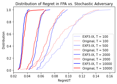
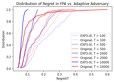
Figure 9: Distribution of regret when using OMD vs its EXP3-IX variant against stochastic and adaptive adversaries for varying $T$.

9.7.3 Stochastic Setting

To verify our algorithms’ theoretical regret guarantees, we consider the setting where the bidder competes in a stochastic setting with multi-unit. Here, the bidder, endowed with valuation vector $\bm{v}=[1,1,1]$, will compete over the course of $T=10^{4}$ rounds for $\overline{M}=M=3$ items. The competing bids are $\bm{b}^{-1}=[0.1,0.1,0.1]$, $[0.3,0.3,1.0]$, or $[0.4,1.0,1.0]$ with probabilities $\frac{1}{4},\frac{1}{4}$, and $\frac{1}{2}$, respectively. Assuming that the bidder receives priority in tiebreaks, with $\mathcal{B}=\{\frac{i}{10}\}_{i\in[10]}$, the expected utility $\sum_{m=1}^{3}$ maximizing bid vector is given by $\bm{b}=[0.4,0.3,0.1]$, which yields utility $(1)(1-0.4)+(0.75)(1-0.3)+(0.5)(1-0.1)=0.6+0.525+0.45=1.575$. We select learning rates $\eta=\sqrt{\tfrac{\log(|\mathcal{B}|)}{|\mathcal{B}|T}}\approx 0.005$ and $\eta=\sqrt{\tfrac{\log(|\mathcal{B}|)}{T}}=0.002$ for the full information and bandit settings respectively (and for the EXP3-IX estimator, we choose an exploration rate of $\sqrt{\frac{2\log(|\mathcal{B}|/\delta)}{4|\mathcal{B}|T}}\approx 0.003$, for high probability bound parameter $\delta=0.05$).

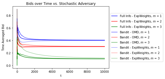
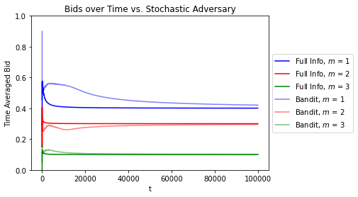
Figure 10: Bid convergence over time under the stochastic setting in Section 9.7.3 for the PAB auction (left) and the uniform price auction (right).

In Figure 10, we plot the average value of each bid over time. Here, the bidder’s objective is to learn the optimal bid vector under each of our three algorithms: decoupled exponential weights algorithm (Algorithm 2) for the full information, modified (i.e., EXP3-IX) version of decoupled exponential weights algorithm (Algorithm 3) for the bandit setting, and modified version of the OMD algorithm (Algorithm 4) for the bandit setting. In this figure, we further compare the rate of convergence to the optimal bid vector of $[0.4,0.3,0.1]$ with our three algorithms. We observe that the full information decoupled exponential weights algorithm converges the fastest to the optimal bid, and the bandit feedback decoupled exponential weights algorithm converges the slowest, and the bandit feedback mirror descent algorithm is in between. This behavior is consistent with our theoretical findings.

We repeat this experiment for the algorithms to learn in uniform price auctions described in Brânzei et al. (2023). Though we do not perform the calculations, the optimal bid vector in the uniform price setting is still $[0.4,0.3,0.1]$. We note that it takes noticeably longer for the bandit algorithm to converge as compared to either its full information variant or our Algorithms 3 or 4, as predicted by the looser regret upper bounds:

Theorem 9.9 ((Discrete) Regret in Uniform Price Auctions, Brânzei et al. (2023))

Under full information feedback (resp. bandit feedback), there exists an algorithm which achieves $O(M^{\frac{3}{2}}\sqrt{T\log|\mathcal{B}|})$ (resp. $O(M^{\frac{5}{2}}|\mathcal{B}|T^{\frac{1}{2}}\log|\sqrt{\log|\mathcal{B}|}+M^{2}\log|\mathcal{B}|)$) discrete regret.

9.8 Uniform Price Market Dynamic Analysis

In this section, we provide some additional experiments or analyses in the market dynamics for the uniform price as prescribed in Section 7.1 in order to directly compare to the dynamics of the PAB auction. In particular, we run a more complete analysis of the uniform price auction bidding dynamics that parallels Section 7.1.

Uniform Price Learning Dynamics: Here, we repeat the setup and analyses of Section 7.1 except using the uniform price auction with bidders bidding according to the learning algorithms as prescribed in Brânzei et al. (2023).

Bid Dynamics. In Figure 11, we observe that the winning bids and largest losing bids noticeably diverge, indicating that the regret minimizing bid strategies are non-uniform (and so are the true hindsight optimal bid vectors which we verified using an offline optimization protocol described in Brânzei et al. (2023)). In particular, as in Section 7.1, there are $N=3$ bidders, $\overline{M}=M=5$ items, the bid space is $\mathcal{B}=\{\frac{i}{20}\}_{i\in[20]}$. The valuations (which are drawn i.i.d. $\text{Unif}(0,1)$ which are then sorted) for this specific instance are given by $\bm{v}_{1}=[0.89,0.7,0.55,0.51,0.29],v_{2}=[0.89,0.44,0.2,0.12,0.05],v_{3}=[0.67,0.64,0.45,0.27,0.02]$. For convenience and ease of comparison, we include the PAB bidding dynamics counterpart (Figure 2) as well.

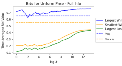
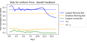
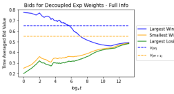
Figure 11: Time averaged bids under market dynamics for the setting described in Section 7.1. The left (resp. right) figures correspond with the full information setting (resp. bandit setting) [and the top (resp. bottom) figures correspond with the uniform price (PAB) auctions. In this specific instance, valuations are given by $\bm{v}_{1}=[0.89,0.7,0.55,0.51,0.29],v_{2}=[0.89,0.44,0.2,0.12,0.05],v_{3}=[0.67,0.64,0.45,0.27,0.02]$].

Welfare and Revenue Over Time. In Figure 12, we compare the distribution of welfare and revenue (normalized by maximum welfare) of the uniform price auction over time showing the 10th, 25th, 50th, 75th, and 90th percentiles in different shades. In particular, we run the full information and bandit feedback learning algorithms for the uniform price auction Brânzei et al. (2023). Note that this figure parallels Figure 5 under PAB. We observe that the welfare rapidly converges to 1 in both the full information and bandit feedback settings. However, the revenue under bandit feedback has noticeably larger variance compared to the full information revenue. Once again, to compare the welfare and revenue evolution over time with the PAB auction, we include the PAB counterpart (Figure 5) for convenience.

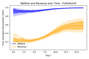
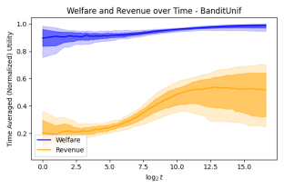
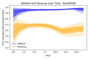
Figure 12: Welfare and revenue over time under the market dynamics for the uniform price auction, under the setting described in Section 7.1. The left (resp. right) figures correspond with the full information setting (resp. bandit setting) and the top (resp. bottom) figures correspond with the uniform price (PAB) auctions.

9.9 Time Varying Valuations

We extend Algorithms 2 and 3 to the time varying valuations setting. In particular, we assume that the valuations $\bm{v}$ are no longer fixed, and instead, in every round $t$, $\bm{v}^{t}$ is independently drawn i.i.d. from some known distribution $F_{\bm{v}}$ with discrete, finite support $\mathcal{V}$. This contextual setting requires a stronger benchmark oracle in comparison to our original setup with a fixed valuation. The new benchmark oracle, which we will formalize shortly, possesses knowledge of the hindsight optimal bid vector for each context. That is, under this benchmark, we have the optimal mapping from any context (valuation vector) to an action (bid vector). Consequently, our current definitions of Regret and $\textsc{Regret}_{\mathcal{B}}$ need to be updated to accommodate these contextual factors:

$$\textsc{Regret}(F_{\bm{v}})=\max_{\bm{b}:\mathcal{V}\to[0,1]^{+M}}\sum_{t=1}^{T}\mathbb{E}_{\bm{v}\sim F_{\bm{v}}}[\mu^{t}_{n}(\bm{b}(\bm{v});\bm{v})]-\mathbb{E}\left[\sum_{t=1}^{T}\mu^{t}_{n}(\bm{b}^{t};\bm{v}^{t})\right]\,.$$ (Continuous Contextual Regret)

Here, $\mu^{t}_{n}(\bm{b};\bm{v})$ denotes the utility of bidder $n$ by submitting bid vector $\bm{b}$ with valuations $\bm{v}$ at round $t$ where the competing bids are $\bm{b}_{-}^{t}$. Observe that in the benchmark of $\textsc{Regret}(F_{\bm{v}})$, i.e., $\max_{\bm{b}:\mathcal{V}\to[0,1]^{+M}}\sum_{t=1}^{T}\mathbb{E}_{\bm{v}\sim F_{\bm{v}}}[\mu^{t}_{n}(\bm{b}(\bm{v});\bm{v})]$, we abuse notation and define valuation-to-bid vector mapping $\bm{b}:\mathcal{V}\to[0,1]^{+M}$. We have an equivalent definition of discretized contextual regret:

$$\textsc{Regret}_{\mathcal{B}}(F_{\bm{v}})=\max_{\bm{b}:\mathcal{V}\to\mathcal{B}^{+M}}\sum_{t=1}^{T}\mathbb{E}_{\bm{v}\sim F_{\bm{v}}}[\mu^{t}_{n}(\bm{b}(\bm{v});\bm{v})]-\mathbb{E}\left[\sum_{t=1}^{T}\mu^{t}_{n}(\bm{b}^{t};\bm{v}^{t})\right]\,.$$ (Discretized Contextual Regret)

An agent’s goal is to minimize their contextual regret with respect to their valuation distribution $F_{\bm{v}}$. Using naive contextual bandit algorithms would lead to a large regret, as the regret of these algorithms scales with the square root of the number of contexts. However, we make an observation that we have complete cross-learning over these contexts as in Balseiro et al. (2022). As such, we borrow from the results described in Balseiro et al. (2022); specifically those explaining the cross-learning-across-contexts generalizations of the EXP3 algorithm in the stochastic contexts (valuations) and adversarial rewards setting (adversarial competing bids).

We assume that the agent has access to their valuation distribution. Moreover, as stated earlier, we assume that the support of this valuation distribution is finite; i.e., $|\mathcal{V}|<\infty$. This scenario occurs often in practice where bidders’ valuations depend naturally on some natural events. For example, investors may prescribe a ‘low’ or ‘high’ value to certain assets depending on various market indices.

We generalize the EXP3-CL algorithm described in Balseiro et al. (2022) to our PAB setting, specifically Algorithm 3, and achieve exactly the same regret rates as our non-contextual variants, albeit requiring an additional $O(|\mathcal{V}|)$ factor of memory and computation.

In order to make the generalization more clear, at a high level, the EXP3-CL algorithm on a set of $K$ arms and $C$ contexts with full cross learning constructs a reward estimator $\hat{r}(k;c)=\frac{r(k;c)}{\sum_{c}\prob(c)\prob(k^{t}=k|c^{t}=c)}\textbf{1}_{k^{t}=k}$ for each arm $k$ and context $c$ pair. Here, the term $\sum_{c}$ is the expected probability that arm $k^{t}=k$ was selected under context $c^{t}=c$, where in the summation we take expectation with respect to the stochasticity over contexts $c$. This estimator mirrors that of standard EXP3 using the IPW estimator, except that the IPW is averaged over the context distribution.

To apply this to our setting, we wish to mimic the behavior of the EXP3-CL algorithm with our decoupled exponential weights algorithm. This can be done by running the EXP3-CL estimator on all of the nodes $b\in\mathcal{B}$ within each layer $m\in[M]$. In particular, we use the following estimator $\widehat{w}_{m}^{t}(b;\bm{v})=1-\frac{1-w_{m}^{t}(b;\bm{v})}{Q_{m}^{t}(b)}\textbf{1}_{b_{m}^{t}=b}$, where the normalizer $Q_{m}^{t}(b)=\sum_{\bm{v}\in\mathcal{V}}$ in this estimator is the expected probability of selecting bid $b$ with corresponding valuation $\bm{v}=\bm{v}^{t}$, where the expectation is taken with respect to all valuation vectors $\bm{v}\in\mathcal{V}$. This procedure, formally described in Algorithm 5 yields the following regret upper bound:

Theorem 9.10 (Time Varying Valuations - Decoupled Exponential Weights)

Under bandit feedback (resp. full information feedback), Algorithm 5, with appropriately chosen $\eta$, achieves contextual continuous regret $\textsc{Regret}(F_{\bm{v}})$ of order $O(M^{\frac{3}{2}}\sqrt{T\log T})$ (resp. $O(M\sqrt{T\log T})$) with total time time and space complexity polynomial in $M$, $|\mathcal{B}|$, $|\mathcal{V}|$, and $T$.

Proof 9.11

Proof of Theorem 9.10

To begin, we can once again ‘decouple’ the utility per unit-bid pair, but this time conditional on the valuation vector context. In particular, we have:

$$\mu_{n}^{t}(\bm{b};\bm{v})=\sum_{m=1}^{M}w_{m}^{t}(b_{m};\bm{v})=\sum_{m=1}^{M}(v_{m}-b_{m})1_{b_{m}\geq b^{t}_{-m}}\quad\text{and}\quad\widehat{\mu}_{n}^{t}(\bm{b};\bm{v})=\sum_{m=1}^{M}\widehat{w}_{m}^{t}(b_{m};\bm{v})\,.$$

As stated earlier, we define reward-weight estimates based on Equation (6) of Balseiro et al. (2022) and our Algorithm 3:

$$\widehat{w}_{m}^{t}(b;\bm{v})=1-\frac{1-w_{m}^{t}(b;\bm{v})}{\sum_{\bm{v}\in\mathcal{V}}\prob(\bm{v}^{t}=\bm{v})q_{m}^{t}(b;\bm{v})}\textbf{1}_{b_{m}^{t}=b}=1-\frac{1-w_{m}^{t}(b;\bm{v})}{Q_{m}^{t}(b)}\textbf{1}_{b_{m}^{t}=b}\,.$$

Here, $q_{m}^{t}(b;\bm{v})=$ is the probability of selecting bid $b$ in slot $m$ with valuation $\bm{v}$. Similarly, $Q_{m}^{t}(b)$ is the probability of selecting bid $b$ for unit $m$, averaged across all possible valuations. One can verify unbiasedness of this estimator $\mathbb{E}[\hat{w}_{m}^{t}(b;\bm{v})]=w_{m}^{t}(b;\bm{v})$ for all $m\in[M],b\in\mathcal{B},\bm{v}\in\mathcal{V}$. The second moment can similarly be computed as:

$$\mathbb{E}[\widehat{w}_{m}^{t}(b;\bm{v})^{2}]=\mathbb{E}\left[\left(1-\frac{1-w_{m}^{t}(b;\bm{v})}{Q_{m}^{t}(b)}\textbf{1}_{b_{m}^{t}=b}\right)^{2}\right]=1-2\mathbb{E}\left[\frac{1-w_{m}^{t}(b;\bm{v})}{Q_{m}^{t}(b)}\textbf{1}_{b_{m}^{t}=b}\right]+\mathbb{E}\left[\left(\frac{1-w_{m}^{t}(b;\bm{v})}{Q_{m}^{t}(b)}\right)^{2}\textbf{1}_{b_{m}^{t}=b}\right]\,.$$

Evaluating the expectations and recalling that $\mathbb{E}[\textbf{1}_{b_{m}^{t}=b}]=Q_{m}^{t}(b)$, we have:

$$\mathbb{E}[\widehat{w}_{m}^{t}(b;\bm{v})^{2}]=1-\left[2-2w_{m}^{t}(b;\bm{v})\right]+\left[\frac{(1-w_{m}^{t}(b;\bm{v}))^{2}}{Q_{m}^{t}(b)}\right]=2w_{m}^{t}(b;\bm{v})-1+\frac{1}{Q_{m}^{t}(b)}\leq 1+\frac{1}{Q_{m}^{t}(b)}\leq\frac{2}{Q_{m}^{t}(b)}\,.$$

Using this, the proof largely follows that of Algorithm 3 up until Equation (LABEL:eq:_full_info_difference). In particular, we have that the contextual regret can be written as:

$$\textsc{Regret}_{\mathcal{B}}(F_{\bm{v}}) =\mathbb{E}_{F_{\bm{v}}}\left[\sum_{t=1}^{T}\mu_{n}^{t}(\bm{b}^{\prime};\bm{v}^{t})-\sum_{t=1}^{T}\mathbb{E}[\mu^{t}(\bm{b}^{t};\bm{v}^{t})]\right]$$

$$\lesssim\eta^{-1}M\log|\mathcal{B}|+\eta\mathbb{E}_{F_{\bm{v}}}\left[\sum_{t=1}^{T}\sum_{\bm{b}}\right]$$

$$=\eta^{-1}M\log|\mathcal{B}|+\eta\left[\sum_{t=1}^{T}\sum_{\bm{v}\in\mathcal{V}}\right]$$

$$=\eta^{-1}M\log|\mathcal{B}|+\eta M\left[\sum_{t=1}^{T}\sum_{m=1}^{M}\sum_{\bm{v}\in\mathcal{V}}\right]$$

$$=\eta^{-1}M\log|\mathcal{B}|+\eta M\left[\sum_{t=1}^{T}\sum_{m=1}^{M}\sum_{\bm{v}\in\mathcal{V}}\right]$$

$$=\eta^{-1}M\log|\mathcal{B}|+2\eta M\left[\sum_{t=1}^{T}\sum_{m=1}^{M}\sum_{\bm{v}\in\mathcal{V}}\right]$$

$$=\eta^{-1}M\log|\mathcal{B}|+2\eta M\left[\sum_{t=1}^{T}\sum_{m=1}^{M}\sum_{b\in\mathcal{B}}\frac{1}{Q_{m}^{t}(b)}\sum_{\bm{v}\in\mathcal{V}}\right]$$

$$=\eta^{-1}M\log|\mathcal{B}|+2\eta M\left[\sum_{t=1}^{T}\sum_{m=1}^{M}\sum_{b\in\mathcal{B}}\frac{1}{Q_{m}^{t}(b)}Q_{m}^{t}(b)\right]$$

$$\leq\eta^{-1}M\log|\mathcal{B}|+\eta M^{2}|\mathcal{B}|T\,.$$

(We will show the first inequality shortly.) With $\eta=\Theta(\sqrt{\frac{\log|\mathcal{B}|}{M|\mathcal{B}|T}})$, this yields the discretized contextual regret upper bounds of $O(M^{\frac{3}{2}}\sqrt{|\mathcal{B}|T\log|\mathcal{B}|})$ under the bandit setting. Accounting for the rounding error of order $O(\frac{MT}{|\mathcal{B}|})$, we obtain the stated continuous contextual regret upper bounds. To obtain the full information results, we simply replace $\widehat{w}_{m}^{t}(b_{m};{\bm{v}}^{t})$ with $w_{m}^{t}(b_{m};{\bm{v}}^{t})$ in the second line of the above equations, which leads to the discretized contextual regret upper bounds of $O(M^{\frac{3}{2}}\sqrt{T\log|\mathcal{B}|})$, as desired.

Next, following the proof of Algorithm 3, we show the first inequality. We define the potentials with respect to a fixed valuation vector $\bm{v}$: $\Phi^{t}(\bm{v})=\sum_{\bm{b}\in\mathcal{B}^{+M}}\exp(\eta\sum_{\tau=1}^{t}\widehat{\mu}^{\tau}(\bm{b};\bm{v}^{\tau}))$. Taking the ratio of adjacent terms, we obtain:

$$\frac{\Phi^{t}(\bm{v})}{\Phi^{t-1}(\bm{v})}=\sum_{\bm{b}\in\mathcal{B}^{+M}}\frac{\exp(\eta\sum_{\tau=1}^{t-1}\widehat{\mu}^{\tau}(\bm{b};\bm{v}^{\tau}))}{\Phi^{t-1}(\bm{v})}\exp(\eta\widehat{\mu}^{t}(\bm{b};\bm{v}^{t}))=\sum_{\bm{b}\in\mathcal{B}^{+M}}$$

Where in the last equality, we used the condition that our algorithm samples bid vector $\bm{b}$ with probability proportional to $\exp(\eta\sum_{\tau=1}^{t-1}\widehat{\mu}^{t}(\bm{b};\bm{v}))$ at round $t$ with valuations $\bm{v}^{t}=\bm{v}$. Combining this with inequalities $\exp(x)\leq 1+x+x^{2}$ and $1+x\leq\exp(x)$ for all $x\leq 1$, we obtain:

$$\frac{\Phi^{t}(\bm{v})}{\Phi^{t-1}(\bm{v})}\leq\sum_{\bm{b}\in\mathcal{B}^{+M}}$$

Combining this with Equations 11 and the fact that $\Phi^{0}(\bm{v})=M\log|\mathcal{B}|$, for any fixed bid vector $\bm{b}^{\prime}$, we have:

$$\sum_{t=1}^{T}\widehat{\mu}^{t}(\bm{b}^{\prime};\bm{v})-\sum_{t=1}^{T}\sum_{\bm{b}} \lesssim\eta^{-1}M\log|\mathcal{B}|+\eta\sum_{t=1}^{T}\sum_{\bm{b}}$$

$$=\eta^{-1}M\log|\mathcal{B}|+\eta\sum_{t=1}^{T}\sum_{\bm{b}}$$

Taking expectations over $\bm{b}$ and the supremum over all $\bm{b}^{\prime}$ yields the desired first crucial regret inequality.

As for the time and space complexity, notice that the only algorithmic difference between Algorithm 5 and Algorithm 3 is precisely in computing the estimator, which in the former, requires having to compute the weights $Q_{m}^{t}(b)$ by iterating over all $\bm{v}\in\mathcal{V}$. As we also have to store reward estimates for each possible valuations, both the time complexity and space complexity of Algorithm 5 are a factor $|\mathcal{V}|$ larger than in Algorithm 3, which are $O(M|\mathcal{B}||\mathcal{V}|T)$ and $O(M|\mathcal{B}||\mathcal{V}|)$ respectively.

Input: Learning rate $0<\eta<\frac{1}{M}$, Valuation Distribution $F_{\bm{v}}$

Output: The aggregate utility $\sum_{t=1}^{T}\mu_{n}^{t}(\bm{b}^{t};\bm{v}^{t})$

$\widehat{W}_{m}^{0}(b;\bm{v})\leftarrow 0$ for all $m\in[M],b\in\mathcal{B},\bm{v}\in\mathcal{V}$ such that $b\leq v_{m}$; else $\widehat{W}_{m}^{0}(b;\bm{v})\leftarrow-\infty$.;

for $t\in[1,\ldots,T]$: do

       Observe Valuation Vector $\bm{v}^{t}\sim F_{\bm{v}}$;

       $b_{0}^{t}\leftarrow\max\mathcal{B}$, and $\widehat{S}_{M+1}^{t}(\min\mathcal{B};\bm{v}^{t})=1$ for any $t\in[T]$;

       Recursively Computing Exponentially Weighted Partial Utilities $\bm{S}^{t}$;

       for $m\in[M,\ldots,1],b\in\mathcal{B}:\widehat{S}^{t}_{m}(b;\bm{v}^{t})\leftarrow\exp(\eta\widehat{W}_{m}^{t}(b;\bm{v}^{t}))\sum_{b^{\prime}\leq b}\widehat{S}_{m+1}^{t}(b^{\prime};\bm{v}^{t})$ $\backslash\backslash$ $\textsc{Compute}-\widehat{S}_{m}$;

       Determining the Bid Vector $\bm{b}^{t}$ Recursively;

       for $m\in[1,\ldots,M],b\leq b_{m-1}^{t}:b_{m}^{t}\leftarrow b$ with probability $\frac{\widehat{S}^{t}_{m}(b;\bm{v}^{t})}{\sum_{b^{\prime}\leq b_{m-1}^{t}}\widehat{S}^{t}_{m}(b^{\prime};\bm{v}^{t})};$   $\backslash\backslash$ $\textsc{Sample}-\bm{b}$;

       Observe $\bm{b}^{t}_{-}$ and receive reward $\mu_{n}^{t}(\bm{b}^{t};\bm{v}^{t})$;

       $Q_{m}^{t}(b)\leftarrow 0$ for all $m\in[M],b\in\mathcal{B}$;

       for $\bm{v}\in\mathcal{V}$: do

             Recursively Computing Probability Measure $\bm{q}$ Under $\bm{v}\in{\mathcal{V}}$;

             $\widehat{S}^{t}_{M+1}(b;\bm{v})\leftarrow 1$ for all $m\in[M],b\in\mathcal{B}$;

             for $m\in[M,\ldots,1],b\in\mathcal{B}:\widehat{S}^{t}_{m}(b;\bm{v})\leftarrow\exp(\eta\widehat{W}_{m}^{t}(b;\bm{v}))\sum_{b^{\prime}\leq b}\widehat{S}_{m+1}^{t}(b^{\prime};\bm{v})$;

             $q^{t}_{1}(b;\bm{v})\leftarrow\frac{\widehat{S}^{t}_{m}(b;\bm{v})}{\sum_{b^{\prime}\in\mathcal{B}}\widehat{S}^{t}_{m}(b^{\prime};\bm{v})}$ for all $b\in\mathcal{B}$;

             for $m\in[2,\ldots,M],b\in\mathcal{B}:q_{m}^{t}(b;\bm{v})\leftarrow\sum_{b^{\prime}\geq b}\frac{q_{m-1}^{t}(b^{\prime};\bm{v})\widehat{S}^{t}_{m}(b;\bm{v})}{\sum_{b"\geq b^{\prime}}\widehat{S}^{t}_{m}(b";\bm{v})}$ for all $b\in\mathcal{B}$;

             $Q_{m}^{t}(b)\leftarrow Q_{m}^{t}(b)+$

       end for

      Update Weight Estimates;

       if Bandit Feedback, for $m\in[M],b\in\mathcal{B},\bm{v}\in\mathcal{V}$;

       $\widehat{W}^{t+1}_{m}(b;\bm{v})\leftarrow\widehat{W}^{t}_{m}(b;\bm{v})+(1-\frac{1-(v-b)\textbf{1}_{b\geq b^{t}_{m}}}{Q_{m}^{t}(b)}\textbf{1}_{b^{t}_{m}=b})$ if $b\leq v$; else $\widehat{W}^{t+1}_{m}(b;\bm{v})\leftarrow-\infty$;

       if Full Information, for $m\in[M],b\in\mathcal{B},\bm{v}\in\mathcal{V}$;

       $\widehat{W}^{t+1}_{m}(b;\bm{v})\leftarrow\widehat{W}^{t}_{m}(b;\bm{v})+(v-b)\textbf{1}_{b\geq b^{t}_{m}}$ if $b\leq v$; else $\widehat{W}^{t+1}_{m}(b;\bm{v})\leftarrow-\infty$;

      

end for

Return $\sum_{t=1}^{T}\mu_{n}^{t}(\bm{b}^{t};\bm{v}^{t})$

ALGORITHM 5 Decoupled EXP3-CL - Time Varying Valuations

References

- (1)
- Abbasi-yadkori et al. (2011) Yasin Abbasi-yadkori, Dávid Pál, and Csaba Szepesvári. 2011. Improved Algorithms for Linear Stochastic Bandits. In Advances in Neural Information Processing Systems, J. Shawe-Taylor, R. Zemel, P. Bartlett, F. Pereira, and K.Q. Weinberger (Eds.), Vol. 24. Curran Associates, Inc. https://proceedings.neurips.cc/paper/2011/file/e1d5be1c7f2f456670de3d53c7b54f4a-Paper.pdf
- Aggarwal et al. (2019) Gagan Aggarwal, Ashwinkumar Badanidiyuru, and Aranyak Mehta. 2019. Autobidding with constraints. In Web and Internet Economics: 15th International Conference, WINE 2019, New York, NY, USA, December 10–12, 2019, Proceedings 15. Springer, 17–30.
- Akbarpour and Li (2020) Mohammad Akbarpour and Shengwu Li. 2020. Credible Auctions: A Trilemma. Econometrica 88, 2 (2020), 425–467. https://doi.org/10.3982/ECTA15925 arXiv:https://onlinelibrary.wiley.com/doi/pdf/10.3982/ECTA15925
- Aoyagi (2003) Masaki Aoyagi. 2003. Bid rotation and collusion in repeated auctions. Journal of Economic Theory 112, 1 (2003), 79–105. https://doi.org/10.1016/S0022-0531(03)00071-1
- Audibert et al. (2011) Jean-Yves Audibert, Sebastien Bubeck, and Gabor Lugosi. 2011. Minimax Policies for Combinatorial Prediction Games. (2011). https://doi.org/10.48550/ARXIV.1105.4871
- Ausubel and Milgrom (2006) Lawrence Ausubel and Paul Milgrom. 2006. The Lovely but Lonely Vickrey Auction. Comb. Auct. 17 (01 2006). https://doi.org/10.7551/mitpress/9780262033428.003.0002
- Ausubel (2004) Lawrence M. Ausubel. 2004. An Efficient Ascending-Bid Auction for Multiple Objects. American Economic Review 94, 5 (December 2004), 1452–1475. https://doi.org/10.1257/0002828043052330
- Ausubel and Cramton (2005) Lawrence M. Ausubel and Peter Cramton. 2005. Dynamic Auctions in Procurement. Handbook of Procurement (2005). https://www.cramton.umd.edu/papers2005-2009/ausubel-cramton-dynamic-auctions-in-procurement.pdf
- Ausubel et al. (2014) Lawrence M. Ausubel, Peter Cramton, Marek Pycia, Marzena Rostek, and Marek Weretka. 2014. Demand Reduction and Inefficiency in Multi-Unit Auctions. The Review of Economic Studies 81, 4 (289) (2014), 1366–1400. http://www.jstor.org/stable/43551738
- Babaioff et al. (2022) Moshe Babaioff, Nicole Immorlica, Yingkai Li, and Brendan Lucier. 2022. Making Auctions Robust to Aftermarkets. arXiv:2107.05853 [econ.TH]
- Badanidiyuru et al. (2021) Ashwinkumar Badanidiyuru, Zhe Feng, and Guru Guruganesh. 2021. Learning to Bid in Contextual First Price Auctions. https://doi.org/10.48550/ARXIV.2109.03173
- Baisa and Burkett (2018) Brian Baisa and Justin Burkett. 2018. Large multi-unit auctions with a large bidder. Journal of Economic Theory 174 (2018), 1–15.
- Balseiro et al. (2022) Santiago Balseiro, Negin Golrezaei, Mohammad Mahdian, Vahab Mirrokni, and Jon Schneider. 2022. Contextual Bandits with Cross-Learning. Mathematics of Operations Research (2022).
- Bartok et al. (2011) G. Bartok, D. P´al, C. Szepesv´ari, and I. Szita. 2011. Online learning. Lecture notes, University of Alberta. (2011). http://david.palenica.com/papers/online-learning-lecture-notes/online-learning-lecture-notes-2011-Oct-20.pdf#page44
- Beyhaghi et al. (2021) Hedyeh Beyhaghi, Negin Golrezaei, Renato Paes Leme, Martin Pál, and Balasubramanian Sivan. 2021. Improved Revenue Bounds for Posted-Price and Second-Price Mechanisms. Operations research. 69, 6 (2021).
- Bigler (2019) Jason Bigler. 2019. An update on first price auctions for Google Ad Manager. (2019). https://blog.google/products/ads-commerce/update-first-price-auctions-google-ad-manager/
- Binmore and Swierzbinski (2000) Ken Binmore and Joe Swierzbinski. 2000. Treasury auctions: Uniform or discriminatory? Review of Economic Design 5 (2000), 387–410.
- Blum et al. (2008) Avrim Blum, MohammadTaghi Hajiaghayi, Katrina Ligett, and Aaron Roth. 2008. Regret Minimization and the Price of Total Anarchy. In Proceedings of the Fortieth Annual ACM Symposium on Theory of Computing (Victoria, British Columbia, Canada) (STOC ’08). Association for Computing Machinery, New York, NY, USA, 373–382. https://doi.org/10.1145/1374376.1374430
- Brânzei et al. (2023) Simina Brânzei, Mahsa Derakhshan, Negin Golrezaei, and Yanjun Han. 2023. Online Learning in Multi-unit Auctions. arXiv:2305.17402 [cs.GT]
- Burkett and Woodward (2020) Justin Burkett and Kyle Woodward. 2020. Uniform price auctions with a last accepted bid pricing rule. Journal of Economic Theory 185 (2020), 104954. https://doi.org/10.1016/j.jet.2019.104954
- Buşoniu et al. (2010) Lucian Buşoniu, Robert Babuška, and Bart De Schutter. 2010. Multi-agent Reinforcement Learning: An Overview. Springer Berlin Heidelberg, Berlin, Heidelberg, 183–221. https://doi.org/10.1007/978-3-642-14435-6_7
- Cai and Daskalakis (2017) Yang Cai and Constantinos Daskalakis. 2017. Learning Multi-item Auctions with (or without) Samples. In FOCS.
- Calvano et al. (2021) Emilio Calvano, Giacomo Calzolari, Vincenzo Denicoló, and Sergio Pastorello. 2021. Algorithmic collusion with imperfect monitoring. International Journal of Industrial Organization 79 (2021), 102712. https://doi.org/10.1016/j.ijindorg.2021.102712
- Chen et al. (2013) Wei Chen, Yajun Wang, and Yang Yuan. 2013. Combinatorial Multi-Armed Bandit: General Framework and Applications. In Proceedings of the 30th International Conference on Machine Learning (Proceedings of Machine Learning Research, Vol. 28), Sanjoy Dasgupta and David McAllester (Eds.). PMLR, Atlanta, Georgia, USA, 151–159. https://proceedings.mlr.press/v28/chen13a.html
- Chu et al. (2011) Wei Chu, Lihong Li, Lev Reyzin, and Robert Schapire. 2011. Contextual Bandits with Linear Payoff Functions. In Proceedings of the Fourteenth International Conference on Artificial Intelligence and Statistics (Proceedings of Machine Learning Research, Vol. 15), Geoffrey Gordon, David Dunson, and Miroslav Dudík (Eds.). PMLR, Fort Lauderdale, FL, USA, 208–214. https://proceedings.mlr.press/v15/chu11a.html
- Cramton (1998) Peter Cramton. 1998. Ascending auctions. European Economic Review 42, 3 (1998), 745–756. https://doi.org/10.1016/S0014-2921(97)00122-0
- Cramton et al. (2004) Peter Cramton, Yoav Shoham, and Richard Steinberg. 2004. Combinatorial Auctions. Papers of Peter Cramton 04mit. University of Maryland, Department of Economics - Peter Cramton. https://ideas.repec.org/p/pcc/pccumd/04mit.html
- Dani et al. (2008) Varsha Dani, Thomas Hayes, and Sham Kakade. 2008. Stochastic Linear Optimization under Bandit Feedback. 355–366.
- de Keijzer et al. (2013a) Bart de Keijzer, Evangelos Markakis, Guido Schäfer, and Orestis Telelis. 2013a. Inefficiency of Standard Multi-unit Auctions. In Algorithms – ESA 2013, Hans L. Bodlaender and Giuseppe F. Italiano (Eds.). Springer Berlin Heidelberg, Berlin, Heidelberg, 385–396.
- de Keijzer et al. (2013b) Bart de Keijzer, Evangelos Markakis, Guido Schäfer, and Orestis Telelis. 2013b. On the Inefficiency of Standard Multi-Unit Auctions. CoRR abs/1303.1646 (2013). arXiv:1303.1646 http://arxiv.org/abs/1303.1646
- Deng et al. (2023) Yuan Deng, Negin Golrezaei, Patrick Jaillet, Jason Cheuk Nam Liang, and Vahab Mirrokni. 2023. Multi-channel Autobidding with Budget and ROI Constraints. arXiv e-prints (2023), arXiv–2302.
- Deospotakis et al. (2021) S. Deospotakis, R. Ravi, and A. Sayedi. 2021. First-Price Auctions in Online Display Advertising. Journal of Marketing Research. Journal of Marketing Research 58(5) (2021), 888–907. https://doi.org/10.1177/00222437211030201
- Derakhshan et al. (2022) Mahsa Derakhshan, Negin Golrezaei, and Renato Paes Leme. 2022. Linear program-based approximation for personalized reserve prices. Management Science 68, 3 (2022), 1849–1864.
- Derakhshan et al. (2021) Mahsa Derakhshan, David M Pennock, and Aleksandrs Slivkins. 2021. Beating greedy for approximating reserve prices in multi-unit VCG auctions. In Proceedings of the 2021 ACM-SIAM Symposium on Discrete Algorithms (SODA). SIAM, 1099–1118.
- Dobzinski and Nisan (2007) Shahar Dobzinski and Noam Nisan. 2007. Mechanisms for Multi-Unit Auctions. In Proceedings of the 8th ACM Conference on Electronic Commerce (San Diego, California, USA) (EC ’07). Association for Computing Machinery, New York, NY, USA, 346–351. https://doi.org/10.1145/1250910.1250960
- Dudík et al. (2017) Miroslav Dudík, Nika Haghtalab, Haipeng Luo, Robert E. Schapire, Vasilis Syrgkanis, and Jennifer Wortman Vaughan. 2017. Oracle-Efficient Learning and Auction Design. In FOCS.
- EEX (2023) EEX. 2023. EU ETS Auctions. (2023). https://www.eex.com/en/markets/environmental-markets/eu-ets-auctions#:~:text=Bids%20are%20sorted%20in%20descending,selection%20according%20to%20an%20algorithm
- Fabra et al. (2006) Natalia Fabra, Nils-Henrik von der Fehr, and David Harbord. 2006. Designing Electricity Auctions. The RAND Journal of Economics 37, 1 (2006), 23–46. http://www.jstor.org/stable/25046225
- Federico and Rahman (2003) Giulio Federico and David Rahman. 2003. Bidding in an Electricity Pay-as-Bid Auction. Journal of Regulatory Economics (2003). https://link.springer.com/article/10.1023/A:1024738128115
- Feldman et al. (2017) Michal Feldman, Brendan Lucier, and Noam Nisan. 2017. Correlated and Coarse equilibria of Single-item auctions. arXiv:1601.07702 [cs.GT]
- Garbade and Ingber (2005) Kenneth Garbade and Jeffrey Ingber. 2005. The Treasury Auction Process: Objectives, Structure, and Recent Adaptations. (2005). https://ssrn.com/abstract=678301
- Goldner et al. (2019) Kira Goldner, Nicole Immorlica, and Brendan Lucier. 2019. Reducing Inefficiency in Carbon Auctions with Imperfect Competition. https://doi.org/10.48550/ARXIV.1912.06428
- Golrezaei et al. (2020) Negin Golrezaei, Patrick Jaillet, and Jason Cheuk Nam Liang. 2020. No-regret learning in price competitions under consumer reference effects. Advances in Neural Information Processing Systems 33 (2020), 21416–21427.
- Golrezaei et al. (2023a) Negin Golrezaei, Patrick Jaillet, and Jason Cheuk Nam Liang. 2023a. Incentive-aware contextual pricing with non-parametric market noise. In International Conference on Artificial Intelligence and Statistics. PMLR, 9331–9361.
- Golrezaei et al. (2023b) Negin Golrezaei, Patrick Jaillet, Jason Cheuk Nam Liang, and Vahab Mirrokni. 2023b. Pricing against a Budget and ROI Constrained Buyer. In International Conference on Artificial Intelligence and Statistics. PMLR, 9282–9307.
- Golrezaei et al. (2021a) Negin Golrezaei, Adel Javanmard, and Vahab Mirrokni. 2021a. Dynamic incentive-aware learning: Robust pricing in contextual auctions. Operations Research 69, 1 (2021), 297–314.
- Golrezaei et al. (2021b) Negin Golrezaei, Max Lin, Vahab Mirrokni, and Hamid Nazerzadeh. 2021b. Boosted second price auctions: Revenue optimization for heterogeneous bidders. In Proceedings of the 27th ACM SIGKDD Conference on Knowledge Discovery & Data Mining. 447–457.
- Goulder and Schein (2013) Larence H. Goulder and Andrew R. Schein. 2013. Carbon Taxes versus Cap and Trade: A Critical Review. Climate Change Economics 4 (2013). https://www.worldscientific.com/doi/10.1142/S2010007813500103
- Gregor (2023) ERBACH Gregor. 2023. Review of the EU ETS: Fit for 55. (2023).
- Han et al. (2020b) Yanjun Han, Zhengyuan Zhou, Aaron Flores, Erik Ordentlich, and Tsachy Weissman. 2020b. Learning to Bid Optimally and Efficiently in Adversarial First-price Auctions. https://doi.org/10.48550/ARXIV.2007.04568
- Han et al. (2020a) Yanjun Han, Zhengyuan Zhou, and Tsachy Weissman. 2020a. Optimal No-regret Learning in Repeated First-price Auctions. https://doi.org/10.48550/ARXIV.2003.09795
- Haoyu and Wei (2020) Zhao Haoyu and Chen Wei. 2020. Online Second Price Auction with Semi-Bandit Feedback under the Non-Stationary Setting. Proceedings of the AAAI Conference on Artificial Intelligence 34, 04 (Apr. 2020), 6893–6900. https://doi.org/10.1609/aaai.v34i04.6171
- Hartline et al. (2014) Jason Hartline, Darrell Hoy, and Sam Taggart. 2014. Price of Anarchy for Revenue. (04 2014).
- Hartline et al. (2015) Jason Hartline, Vasilis Syrgkanis, and Eva Tardos. 2015. No-Regret Learning in Bayesian Games. In Advances in Neural Information Processing Systems, C. Cortes, N. Lawrence, D. Lee, M. Sugiyama, and R. Garnett (Eds.), Vol. 28. Curran Associates, Inc. https://proceedings.neurips.cc/paper/2015/file/3e7e0224018ab3cf51abb96464d518cd-Paper.pdf
- Heim and Götz (2021) Sven Heim and Georg Götz. 2021. Do Pay-As-Bid Auctions Favor Collusion? Evidence from Germany’s market for reserve power. Energy Policy 155 (2021), 112308. https://doi.org/10.1016/j.enpol.2021.112308
- Hendricks and Porter (1989) Kenneth Hendricks and Robert H. Porter. 1989. Collusion in Auctions. Annales d’Économie et de Statistique 15/16 (1989), 217–230. http://www.jstor.org/stable/20075758
- Hortaçsu and McAdams (2010) Ali Hortaçsu and David McAdams. 2010. Mechanism Choice and Strategic Bidding in Divisible Good Auctions: An Empirical Analysis of the Turkish Treasury Auction Market. Journal of Political Economy 118, 5 (2010), 833–865. http://www.jstor.org/stable/10.1086/657948
- Huang et al. (2018) Zhiyi Huang, Jinyan Liu, and Xiangning Wang. 2018. Learning Optimal Reserve Price against Non-myopic Bidders. https://doi.org/10.48550/ARXIV.1804.11060
- Kanoria and Nazerzadeh (2014) Yash Kanoria and Hamid Nazerzadeh. 2014. Dynamic Reserve Prices for Repeated Auctions: Learning from Bids. In Web and Internet Economics: 10th International Conference, WINE 2014, Beijing, China, December 14-17, 2014, Proceedings, Vol. 8877. Springer, 232.
- Kolumbus and Nisan (2022) Yoav Kolumbus and Noam Nisan. 2022. Auctions between Regret-Minimizing Agents. In Proceedings of the ACM Web Conference 2022 (Virtual Event, Lyon, France) (WWW ’22). Association for Computing Machinery, New York, NY, USA, 100–111. https://doi.org/10.1145/3485447.3512055
- Koolen et al. (2010) Wouter M Koolen, Manfred K Warmuth, and Jyrki Kivinen. 2010. Hedging Structured Concepts. Conference on Learning Theory 23 (2010), 93–105.
- Lattimore and Szepesvári (2020) Tor Lattimore and Csaba Szepesvári. 2020. Bandit Algorithms. Cambridge University Press. https://doi.org/10.1017/9781108571401
- Littlestone and Warmuth (1994) Nick Littlestone and Manfred K. Warmuth. 1994. The Weighted Majority Algorithm. Inf. Comput. 108, 2 (1994), 212–261. https://doi.org/10.1006/inco.1994.1009
- Lucier and Borodin (2009) Brendan Lucier and Allan Borodin. 2009. Price of anarchy for greedy auctions. In ACM-SIAM Symposium on Discrete Algorithms.
- Lucier et al. (2023) Brendan Lucier, Sarath Pattathil, Aleksandrs Slivkins, and Mengxiao Zhang. 2023. Autobidders with budget and roi constraints: Efficiency, regret, and pacing dynamics. arXiv preprint arXiv:2301.13306 (2023).
- Lykouris et al. (2016) Thodoris Lykouris, Vasilis Syrgkanis, and Éva Tardos. 2016. Learning and Efficiency in Games with Dynamic Population. In Proceedings of the Twenty-Seventh Annual ACM-SIAM Symposium on Discrete Algorithms (Arlington, Virginia) (SODA ’16). Society for Industrial and Applied Mathematics, USA, 120–129.
- Mohri and Medina (2013) Mehryar Mohri and Andres Muñoz Medina. 2013. Learning Theory and Algorithms for Revenue Optimization in Second-Price Auctions with Reserve. https://doi.org/10.48550/ARXIV.1310.5665
- Mohri and Medina (2015) Mehryar Mohri and Andrés Muñoz Medina. 2015. Revenue Optimization against Strategic Buyers. In NIPS.
- Mohri and Medina (2016) Mehryar Mohri and Andrés Munoz Medina. 2016. Learning algorithms for second-price auctions with reserve. The Journal of Machine Learning Research 17, 1 (2016), 2632–2656.
- Morgenstern and Roughgarden (2016) Jamie Morgenstern and Tim Roughgarden. 2016. Learning Simple Auctions. In 29th Annual Conference on Learning Theory (Proceedings of Machine Learning Research, Vol. 49), Vitaly Feldman, Alexander Rakhlin, and Ohad Shamir (Eds.). PMLR, Columbia University, New York, New York, USA, 1298–1318.
- Nautz (1995) D. Nautz. 1995. Optimal bidding in multi-unit auctions with many bidders. Economics Letters 48, 3 (1995), 301–306. https://doi.org/10.1016/0165-1765(94)00641-E
- Nedelec et al. (2019) Thomas Nedelec, Noureddine El Karoui, and Vianney Perchet. 2019. Learning to bid in revenue-maximizing auctions. CoRR abs/1902.10427 (2019). arXiv:1902.10427 http://arxiv.org/abs/1902.10427
- Neu (2015) Gergely Neu. 2015. Explore no more: Improved high-probability regret bounds for non-stochastic bandits. arXiv:1506.03271 [cs.LG]
- Niazadeh et al. (2022) Rad Niazadeh, Negin Golrezaei, Joshua Wang, Fransisca Susan, and Ashwinkumar Badanidiyuru. 2022. Online Learning via Offline Greedy Algorithms: Applications in Market Design and Optimization. Management Science (2022).
- Pesendorfer (2000) Martin Pesendorfer. 2000. A Study of Collusion in First-Price Auctions. The Review of Economic Studies 67, 3 (2000), 381–411. http://www.jstor.org/stable/2566959
- Phelps et al. (2008) Steve Phelps, Kai Cai, Peter McBurney, Jinzhong Niu, Simon Parsons, and Elizabeth Sklar. 2008. Auctions, Evolution, and Multi-agent Learning. In Adaptive Agents and Multi-Agent Systems III. Adaptation and Multi-Agent Learning, Karl Tuyls, Ann Nowe, Zahia Guessoum, and Daniel Kudenko (Eds.). Springer Berlin Heidelberg, Berlin, Heidelberg, 188–210.
- Porter et al. (2003) David Porter, Stephen Rassenti, Anil Roopnarine, and Vernon Smith. 2003. Combinatorial auction design. Proceedings of the National Academy of Sciences 100, 19 (2003), 11153–11157. https://doi.org/10.1073/pnas.1633736100 arXiv:https://www.pnas.org/doi/pdf/10.1073/pnas.1633736100
- Pycia and Woodward (2020) Market Pycia and Kyle Woodward. 2020. Auctions of Homogeneous Goods: A Case for Pay-as-Bid. (2020). https://ssrn.com/abstract=3865760orhttp://dx.doi.org/10.2139/ssrn.3865760
- Rakhlin (2009) Alexander Rakhlin. 2009. Lecture Notes on Online Learning. (2009). https://www.mit.edu/~rakhlin/papers/online_learning.pdf
- Roughgarden (2015) Tim Roughgarden. 2015. The Price of Anarchy in Games of Incomplete Information. ACM Trans. Econ. Comput. 3, 1, Article 6 (mar 2015), 20 pages. https://doi.org/10.1145/2737816
- Roughgarden et al. (2017) Tim Roughgarden, Vasilis Syrgkanis, and Éva Tardos. 2017. The Price of Anarchy in Auctions. J. Artif. Int. Res. 59, 1 (may 2017), 59–101.
- Roughgarden and Wang (2016) Tim Roughgarden and Joshua R. Wang. 2016. Minimizing Regret with Multiple Reserves. In Proceedings of the 2016 ACM Conference on Economics and Computation, EC ’16, Maastricht, The Netherlands, July 24-28, 2016. 601–616.
- Schmalensee and Stavins (2017) Richard Schmalensee and Robert N. Stavins. 2017. Lessons Learned from Three Decades of Experience with Cap and Trade. Review of Environmental Economics and Policy 11 (2017). https://www.journals.uchicago.edu/doi/full/10.1093/reep/rew017
- Susan et al. (2023) Fransisca Susan, Negin Golrezaei, and Okke Schrijvers. 2023. Multi-Platform Budget Management in Ad Markets with Non-IC Auctions. arXiv preprint arXiv:2306.07352 (2023).
- Syrgkanis and Tardos (2012) Vasilis Syrgkanis and Eva Tardos. 2012. Composable and Efficient Mechanisms. arXiv:1211.1325 [cs.GT]
- Takimoto and Warmuth (2003) Eiji Takimoto and Manfred K. Warmuth. 2003. Path Kernels and Multiplicative Updates. J. Mach. Learn. Res. 4, null (dec 2003), 773–818.
- Tierney et al. (2008) Susan Tierney, Todd Schatzki, and Rana Mukerji. 2008. Uniform-Pricing versus Pay-as-Bid in Wholesale Electricity Markets: Does it Make a Difference? (2008). https://kylewoodward.com/blog-data/pdfs/references/tierney+schatzki+mukerji-new-york-iso-2008A.pdf
- Tsybakov (2008) Alexandre B. Tsybakov. 2008. Introduction to Nonparametric Estimation (1st ed.). Springer Publishing Company, Incorporated.
- Van Parys and Golrezaei (2023) Bart PG Van Parys and Negin Golrezaei. 2023. Optimal learning for structured bandits. Management Science (2023).
- Yang and Wang (2020) Yaodong Yang and Jun Wang. 2020. An Overview of Multi-Agent Reinforcement Learning from Game Theoretical Perspective. CoRR abs/2011.00583 (2020). arXiv:2011.00583 https://arxiv.org/abs/2011.00583
- Zhang et al. (2021) Kaiqing Zhang, Zhuoran Yang, and Tamer Başar. 2021. Multi-Agent Reinforcement Learning: A Selective Overview of Theories and Algorithms. Springer International Publishing, Cham, 321–384. https://doi.org/10.1007/978-3-030-60990-0_12
- Zimin and Neu (2013) Alexander Zimin and Gergely Neu. 2013. Online learning in episodic Markovian decision processes by relative entropy policy search. In Advances in Neural Information Processing Systems, C.J. Burges, L. Bottou, M. Welling, Z. Ghahramani, and K.Q. Weinberger (Eds.), Vol. 26. Curran Associates, Inc. https://proceedings.neurips.cc/paper/2013/file/68053af2923e00204c3ca7c6a3150cf7-Paper.pdf