Causative Cyberattacks on Online Learning-based Automated Demand Response Systems
Abstract
Power utilities are adopting Automated Demand Response (ADR) to replace the costly fuel-fired generators and to preempt congestion during peak electricity demand. Similarly, third-party Demand Response (DR) aggregators are leveraging controllable small-scale electrical loads to provide on-demand grid support services to the utilities. Some aggregators and utilities have started employing Artificial Intelligence (AI) to learn the energy usage patterns of electricity consumers and use this knowledge to design optimal DR incentives. Such AI frameworks use open communication channels between the utility/aggregator and the DR customers, which are vulnerable to causative data integrity cyberattacks. This paper explores vulnerabilities of AI-based DR learning and designs a data-driven attack strategy informed by DR data collected from the New York University (NYU) campus buildings. The case study demonstrates the feasibility and effects of maliciously tampering with (i) real-time DR incentives, (ii) DR event data sent to DR customers, and (iii) responses of DR customers to the DR incentives.
Index Terms:
Causative attacks, cybersecurity, demand response, shapley value, smart grids.I Introduction
Internet-of-Things (IoT) enable power utilities to adopt Demand Response (DR) strategies to reduce or shift electricity demand peaks. Thus, in 2018, the US utilities used 4.5% of the peak load capacity for DR services. This is estimated to increase to 20% in 2030 yielding annual cost savings of $15 billion [1]. The DR resources vary from electricity-dependent industrial processes (e.g., steel industry and irrigation control) to high-wattage residential appliances (e.g., Electric Vehicles (EVs), air-conditioners, and refrigerators). DR is either managed directly by the utilities or by third-party, for-profit DR aggregators. For example, there are third-party aggregators in California, US that cooperate with local power utilities [2, 3].
The utilities and aggregators are automating interactions with their DR-enabled customers. By default, Automated Demand Response (ADR) does not require human intervention to optimize, schedule, and exercise DR capacity. However, interventions are possible. The most common standard for automated communication between DR customers and an aggregator or utility is the Open Automated Demand Response (OpenADR), which is recognized by the International Electrotechnical Commission (IEC) [4]. The OpenADR standard defines the two ends of a communication channel as the Virtual Top Node (VTN) and the Virtual End Node (VEN), issues digital certificates to the nodes for an authenticated communication, and encrypts information exchanged between the nodes. Despite the standardization and the use of industry-grade encryption, cyber threats in ADR prevail because DR customers lack industry-grade cyber defense and hygiene on their devices.
Widely deployed Smart Meters (SMs) and Building Energy Management Systems (BEMSs), i.e., VENs in the OpenADR framework are vulnerable to cyberattacks. SMs and BEMSs use wireless communication technologies (e.g., WiFi, ZigBee, BACnet, and ModBus) to interface within a co-located area or a building and use Wide Area Networks (WAN) such as cellular networks and Power Line Communication (PLC) to interface with the utilities or aggregators [5, 6, 7]. Attackers can exploit vulnerabilities in the communication technologies (e.g., WiFi [8], ZigBee [9]) to compromise SMs and BEMSs. On the other hand, cellular networks and PLC are vulnerable to man-in-the-middle cyberattacks [10].
In addition to vulnerabilities in the ADR, SMs are vulnerable to remote cyberattacks compromising data privacy, causing Denial-of-Service (DoS), and enabling power theft [11, 12, 13, 14]. Physical accessibility of SMs increases their attack surface, which can be defined as the total number of vulnerable devices and processes. Tabrizi et al. [14] acknowledge the importance of physical access to SMs for successful DoS and data tampering attacks. Attack surfaces of SMs and BEMSs can be increased by malicious smart appliances (e.g., smart television, smart lights and EVs [15]) connected to the same network. Since these smart appliances have complex, opaque and porous supply chains, attackers can exploit these supply chains to compromise SMs and BEMSs. For instance, the US Federal Bureau of Investigation (FBI) alarmed the private sector in February 2020 about Kwampirs, a remote access malware that infects the supply chains of the software products related to the US energy sector [16]. Although these attacks have not been encountered at scale, their possibility has lead to investigating the feasibility of demand-side cyberattacks on power grids.
Recent studies [17, 18, 19] considered demand-side cyberattacks on power grids launched by manipulating EVs and Heating, Ventilation, and Air-Conditioning (HVAC) units. Acharya et al. [17] demonstrated that public power grid and commercial EV Charging Stations (EVCSs) data can be weaponized to launch remote attacks on the power grid. The study collected public data from documents and websites of the local power utility and their affiliates in Manhattan, New York. The main result in [17] is that a botnet compromising modern EVs charging at kW EVCSs can cause over-frequency in the power grid, tripping a generator cascading into an urban brownout. Authors in [18, 19] analyzed demand-side cyberattacks launched by tampering with generic HVAC appliances. These studies were performed on IEEE test systems and reported frequency instability and line overloading, causing cascading outages and a dramatic increase in the operating costs for the power grid. Raman et al. [20] presented attacks manipulating behavior of DR customers, with the intention of depleting system reserves and corrupting voltage profiles. The common thread of the attacks in [17, 18, 19, 20] is their focus on manipulations of demand-side appliances during DR events assuming that an utility/aggregator does not use AI to learn and monitor DR behavior. With the proliferation of DR customers and advances in AI, such learning and monitoring solutions have become available [21, 22, 23, 24] and practiced (e.g., [25]).
Khezeli and Bitar [21] have developed a learning scheme to dynamically calculate the monetary incentives paid to DR customers to minimize the risk exposure of the utility facing an a priori uncertain response of DR customers. Li et al. [22] extended the approach in [21] to a distributed learning environment using the aggregated DR response of customers, thus avoiding the need to observe individual DR customers. In Meith and Dvorkin [23] and Tucker et al. [24] the approaches in [21] and [22] have been extended to accommodate learning subject to distribution network constraints. The common thread in [21, 22, 23, 24] is that learning is myopic to cyber vulnerabilities of the DR resources, thus assuming that monetary incentives generated by learning are benign, i.e., DR operations are not affected by corrupt data. In contrast, this paper investigates cyberattacks on the DR learning111Information required for the aggregated learning is publicly available. The aggregated DR data and incentives are available via smartphone apps to the DR customers. Public data is an attack vector in the urban power grids, [17]. schemes (e.g., in [21, 22, 23, 24]), which are known as causative attacks in the AI and cybersecurity communities.
Causative attacks denote malicious alterations of input or training data that cause a malfunction of the underlying learner and lead to unintended, erroneous learning outcomes [26, 27]. Mei and Zhu [26] presented a framework to identify possible causative attacks on the learner via a bi-level optimization model, where the upper level models a learner and the lower level models an attacker. The bi-level optimization is solved offline to return the optimal training data alteration to achieve a given attack goal, which is then fed into a targeted decision-making process. Liu et al. [27] consider online causative attacks on machine teaching, where an attacker sequentially feeds the malicious training data to the learner. Online causative attacks are more relevant for the DR learning context because DR operations are sequential in nature and benefit from an iterative learning process (e.g., as presented in [21, 22, 23]).
In the context of related cyberattacks summarized in Table I, this paper makes three contributions:
-
1.
It analyzes cyber vulnerabilities of a state-of-the-art DR learning set up that can be used by either a power utility or an aggregator.
- 2.
-
3.
Using real-life data on DR power curtailment and incentives from the NYU microgrid and buildings, it simulates an attack under conditions similar to US electric power distribution systems to assess the impact of causative attacks on the monetary incentives designed by a utility/DR aggregator. Furthermore, technical challenges such as changes in peak demand and frequency excursions imposed to the power utility are investigated. Finally, we anticipate that the paper raises awareness about implications of causative cyberattacks on ML-enabled and IoT-powered DR programs, thus contributing to striking the consensus among concerned parties (e.g., regulators, power utilities, third-party aggregators, and electricity consumers).
[!t] Attack Attack Vector Paper DS C [9, 10] ✓ Communication protocols, e.g., WiFi, ZigBee. [11, 12, 13, 14] ✓ Smart Meters (SMs) and IoT devices. [17] ✓ Public data on EVs and power grid. [18, 19] ✓ Generic demand-side high-power devices. [20] ✓ Behavior of DR customers. [26] ✓ Training data for underlying offline Machine Learning (ML). [27] ✓ Training data for underlying online ML. This paper ✓ ✓ Causative demand-side attack on DR ML.
II Demand Response Framework in Smart Grids
II-A DR Architecture
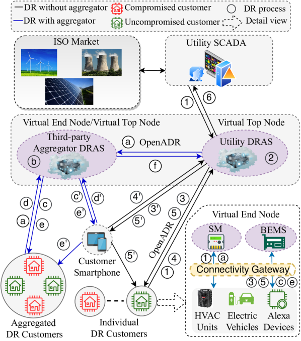
Fig. 1 shows a schematic of the learning-based ADR program employed by either an utility or a third-party DR aggregator. The DR program has six processes (PR.). First, a Demand Response Automated Server (DRAS) acquires real-time energy usage data of DR customers from their individual SMs via the cellular networks and PLC (PR. 1). DRAS receives power grid operational schedules from the utility or, in rare instances, from the Independent System Operator (ISO) via the fiber optic communication lines and cellular networks (PR. 1). Second, the DRAS runs a DR scheduling and pricing algorithm (e.g., heuristic or ML-based) on the collected SM and power grid data (PR. 2). Third, the DR price signals and schedules are sent to the DR customers using OpenADR 2.0 protocol222In OpenADR, the DRAS is a VTN and the DR customer is a VEN. (PR. 3). Alternatively, this information is sent to the DR customers via the customer smartphone app (PR. 3’). Fourth, the DRAS or the VTN receives the responses of the DR customers to the DR call via the OpenADR protocol (PR. 4). This response includes an acknowledgement of receipt of the DR call, accept/reject notice to participate in the DR event, and an estimate of the power available from that VEN. Alternatively, the DR customers can respond via a smartphone app (PR. 4’). Fifth, after accepting the DR call, the VTN can control the DR resources registered in the ADR program, by directly communicating/coordinating with a local BEMS (PR. 5). DR customers can overrule the ADR commands generated by the VTN and control the real-time operations of DR resources via a smartphone app (PR. 5’). Finally, the DRAS sends real-time DR information to the utility (PR. 6).
As shown in Fig. 1, third-party aggregators use DR techniques (PR. a-f) similar to the utilities with two exceptions. First, the aggregator DRAS bids and reports available DR services to the utility DRAS, instead of the ISO market. Second, they use proprietary communication protocols that maybe vulnerable to cyberattacks. The DR aggregators are vital as power utilities have started commonly employing for-profit, third-party aggregators as DR providers to serve three purposes: i) to aggregate small-scale and distributed residential DR resources and provide flexibility to the utility at bulk, ii) to transfer the risk associated with DR uncertainty to the aggregators, and (iii) in some cases, to intensify distribution deregulation [32, 33].
II-B Causative Attack on ML-Based DR
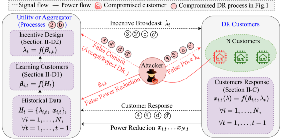
Fig. 2 shows the vulnerabilities introduced by the participants in a DR program. These vulnerabilities can be used to launch causative attacks on ML-enabled DR in Fig. 1. For instance, an attacker can tamper with the DR schedules and incentives sent to the DR customers (PR. 3, 3’, c, and c’). They can manipulate the response of the DR customers to the DR calls (PR. 4, 4’, d, and d’). They can interfere with the power reduced by DR customers during the DR events. By feeding erroneous signals and data to the utility/aggregator DRAS ML model (PR. 2 and b), it impedes the model from learning the true behaviors of DR customers. The model may recommend subpar DR incentives undermining the DR program.
II-C DR Customer Model
This section provides a mathematical model of an individual DR customer based on [23]. The utility function of a DR customer can be modeled as a quadratic function of its power consumption [34, 23, 21, 22]:
| (1) |
where is the power consumed by a DR customer at time , and , are coefficients representing the energy use behavior of the DR customer at time . This utility function quantifies the satisfaction of a DR customer for consuming power at time . Alternatively, it is a measure of cost or dissatisfaction of the DR customer for not consuming power at time . As explained in Section II-A, DR programs make it possible for DR customers to define dissatisfaction tolerance and incentivize them.
In a typical DR program, an utility/aggregator broadcasts a DR incentive ($/kWh) that the DR customer receives by taking part in a DR event scheduled for time . By agreeing to reduce its power consumption by (kW), the DR customer receives a reward ($). Each DR customer optimizes its trade-off between the reward received and the dissatisfaction incurred by power reduction. The objective function of DR customer for a DR event at time is:
| (2) |
From the first order optimality condition, the optimal demand reduced by the DR customer in response to is:
| (3) |
where coefficients and are the price sensitivity of DR customer at DR event .
II-D Utility/Aggregator Model
A rational DR customer reduces its power consumption for a given according to the optimality condition in Eq. (3) [35]. The utility/aggregator expects all their DR customers to reduce their power consumption as follows:
| (4) |
where is the expectation operator and is the number of DR customers participating in the DR program. However, this optimal response is subject to exogenous disturbances pertaining to behavioral aspects of the power consumption of each DR customer and changes in power grid operations (e.g., due to demand forecasting errors). Thus, the utility/aggregator does not know exactly, and hence, can use ML techniques to internalize this stochasticity in the DR. The actual demand reduced by a DR customer during a DR event at time is:
| (5) |
where is an exogenous disturbance (error) added to the optimal response provided by the customer for the DR event at time . The utility/ aggregator observes if and only if vector is known to them. However, the utility/aggregator does not know the vector a priori and learn them [23]. The utility/aggregator must learn the elements of vector , (exploration) to design a proper DR incentive at time (exploitation), as shown in Fig. 2. Exploration and exploitation can happen simultaneously [21, 22, 23]. We show a way to learn as a function of and .
II-D1 Online Exploration of the Utility Function of DR Customers
In the set up of Fig. 2, the utility or aggregator can sequentially record broadcasted DR incentives and reductions in power consumption of the DR customers in response to the incentives. Using this recorded data, , where , , , and , the utility or aggregator estimates by minimizing the Mean Squared Error (MSE) of the expected response of DR customers given by Eq. (5). This objective can be parameterized by the empirical loss function:
| (6a) | ||||
| The first order optimality condition of over is expressed as: | ||||
| (6b) | ||||
| (6c) | ||||
| Solving Eqs. (6b) and (6c) and setting and , it follows: | ||||
| (6d) | ||||
| (6e) | ||||
| Since set is updated at every DR event at time , Eqs. (6d) and (6e) use streaming historical data to estimate . This is computationally unattractive for all DR customers over time due to the addition of new data points at each DR event at time . To overcome the computational complexity, the utility or aggregator can use the online gradient descent to update for a DR event at time as: | ||||
| (6f) | ||||
where is a user-defined model learning rate and vector . In the setting of Eq. (6f), obtained in Eqs. (6d) and (6e) can be realized as , which is updated at time to based on the new sample set of the DR event at time .
II-D2 Online Exploitation of the DR Incentives
This section builds up the DR incentive design mechanism adopted from [22] and similar to [23, 21]. Using the learning model in Section II-D1, the utility or aggregator can design DR incentives as shown in Fig. 2. We set up the exploitation stage of the DR learning problem from the aggregator viewpoint (a more general case). The aggregator mediates between DR customers and the utility and offers its capacity to the utility at a pre-defined price ahead of DR event. During the DR event, the aggregator must supply the offered capacity from its portfolio of DR customers, while maximizing its DR revenue and minimizing the dissatisfaction to the DR customers. For a DR event at time , objective of the aggregator is:
| (7a) | ||||
| where we omitted subscript as we focus on one particular DR event in rest of the this section. The first term in Eq. (7a) accounts for the penalty of not delivering the committed DR capacity to the utility ( kW), the second term represents the revenue collected by the DR aggregator from the utility for the provided DR services, and the third term is the expected utility function of the DR customers. Notably, these terms are normalized by a factor of for mathematical tractability. Parameters and denote the per-unit penalty price and the per-unit revenue received from providing DR services to the utility, respectively. Also, disturbance is independent of other customers and events, and hence, is assumed to follow a normal distribution , i.e., and variance [36, 22, 21, 23]. | ||||
Using the first order optimality condition in Eq. (7a), the optimal demand reduced by a DR customer is:
| (7b) |
where and . The DR incentive that the aggregator needs to set for the optimal power reduction in Eq. (7b) can be determined by replacing in Eq. (7a) by an auxiliary variable , i.e., . This replacement constructs an equality constraint for the aggregator to satisfy its DR commitment, and the dual variable of this constraint () returns the optimal DR incentive [22]. Thus, Eq. (7a) is recast as the following constrained optimization:
| (7c) |
Upon solving Eq. (7c), the optimal response is obtained as:
| (7d) |
Comparing Eq. (7b) with Eq. (7d), and indexing for DR event at time , the optimal value of is given by:
| (7e) |
Since in Eq. (7e) is derived from a normalized formulation in Eq. (7a), the actual that needs to be broadcast to DR customers is . The expression in Eq. (7e) parameterizes the exploitation stage of , which can be derived and leveraged by an attacker to launch a causative attack on the DR learning deployed by utility or aggregator.
Remark 1: Eq. (7e) yields a time-varying value of designed by the utility/aggregator. An attacker can compromise this incentive signal and intentionally deviate DR customers from their optimal power consumption reduction. Further, this attack can feed erroneous values of and to a ML algorithm used by the DRAS, which will in turn lead to sub-optimal values of for future DR events. However, if the utility/aggregator elects to use fixed (time-invariable) values of (e.g., for price-insensitive DR customers with constant cost functions) without using a ML algorithm leveraging historical and , there will be no causative attack on the learning process for DR incentives. Additionally, in the case of time-invariable and a priori known values of , the utility/aggregator need not broadcast in real-time. However, even in this case, some attacks on DR signals are still possible (e.g, on DR time and duration– see PR. 3, 3’, c, and c’ in Fig. 1). Although time-invariable and a priori known DR incentives may have a smaller attack surface than the case with time-variable incentives considered in this paper, the latter one dominates across DR programs as it offers greater economic advantage to both the utility/aggregator and DR customers [32, 23, 37].
III Attack Design and Implementation
III-A Devising an Attack
The attacker can launch causative attacks in an online or offline fashion. In the former attack, erroneous data on and are sequentially fed to the ML algorithm operationalized on the DRAS by launching false data injection attacks on the DR schedules, DR incentives, and customer responses to DR calls. Due to the price sensitivity of power reductions to these manipulations, as given by a relationship in Eq. (3), the DRAS is caused to involuntarily produce erroneous outcomes on DR schedules and incentives. In the offline attack, the attacker compromises the DRAS and manipulates the historical training data set on and . In either case, the ML algorithm used in the DRAS learns an erroneous customer behavior and designs a suboptimal DR incentive.
III-B Impact
Attacks on DR learning are of interest to both state and non-state actors; however, their goals and motives differ. For example, state actors may employ such attacks to compromise operations of the national power grid, a critical infrastructure system, while non-state (individual or group) actors can be driven by ransomware. As a result, both attacks from state and non-state actors can inadvertently or intentionally reduce attractiveness of DR programs. For example, such attacks not only can make the utility/aggregators apathetic to continuing existing and rolling-out new DR programs, but also contribute to imposing various operational challenges (e.g., frequency and voltage excursions). Furthermore, such attacks may deteriorate credibility of DR programs among DR customers, thus discouraging them from participation.
III-C Mathematical Formulation
In this section, we describe a mathematical model for designing such aforementioned cyberattacks and analyzes how many DR events and DR customers need to be compromised. We consider the perspective of an attacker and cast its decision-making process as an optimization problem, to determine the number of DR events and DR customers to launch a causative attack on the ML-based ADR employed by the aggregator presented in Section II-D.
Consider an attacker that forces the aggregator to learn the anomalous behavior of DR customers as legitimate responses by tampering with the power curtailment of the compromised DR customers , where and are the compromised set of DR customers and events, respectively. Historical DR data is defined for the DR events up to time , and the attacks are devised starting from DR event at . Notably, for the offline attack scheme described in Section III-A we enforce . The optimization can be formulated as a bi-level problem, where the top-level considers the perspective of the attacker and the lower-level considers the perspective of the DR incentive design by the aggregator. Since the objective of the lower-level problem is to return an optimal (derived in Eq. (7e)), we can express the single-level equivalent as a non-linear, non-convex optimization problem:
| (8a) | ||||
| (8b) | ||||
| (8c) | ||||
| (8d) | ||||
| (8e) | ||||
| (8f) | ||||
| (8g) | ||||
| (8h) | ||||
| (8i) | ||||
| (8j) | ||||
where , and are the maximum power curtailment capacities of compromised and uncompromised DR customers, respectively. Eqs. (8a)-(8i) are upper-level formulations of the bi-level problem. Eq. (8j) is an optimal return of the lower-level problem. Eq. (8a) defines the objective of the attacker, where it forces the aggregator to learn the value defined by the attacker. The attacker can conservatively estimate based on its knowledge of the aggregated . To calculate , an attacker can leverage the aggregated realization of Eq. (3) expressed as:
| (9) |
where and and and then use Eq. (6). Interestingly, the aggregated model only requires knowledge of and , which are publicly available (e.g., via smartphone apps of DR customers and utility documents [38]). Eqs. (8) and (8c) are update rules for using the online gradient method discussed in Eq. (6f) for the compromised and uncompromised DR customers, respectively. Similarly, Eqs. (8d) and (8e) enforce the bounds of customers’ DR capacity. Eq. (8f) constrains the total curtailment commitment of the DR aggregator within a tolerable amount of aggregated error . Eqs. (8g) and (8h) are the curtailed power of compromised and uncompromised DR customers, respectively. Eq. (8i) is a vector assignment of an optimal DR incentive.
In the offline attack case, the attacker compromises the DRAS to access data set , hyperparameter , aggregated DR , and power curtailment limits of DR customers that are needed to solve Eq. (8). On the other hand, to solve Eq. (8) in the online attack case, the attacker needs to know , , and in advance. Notably, the attacker may use to estimate . Solving the optimization in Eq. (8) requires a two-dimensional search across sets and with non-linear and non-convex constraints. This requirement can be fulfilled by either compromising a large fraction of DR customers over a few DR events or by compromising a small fraction of DR customers over a larger number of DR events. This trade-off between the compromised number of DR customers and DR events is idiosyncratic to attackers and the learning scheme employed by the aggregator. To prune the search space and to invoke a pragmatic attack scenario, we solve Eq. (8) by fixing either or . This is in line with the inability of the attacker to compromise a larger number of DR customers for a large number of DR events.
The ease with which residential DR customers can be compromised depends on defense mechanisms employed by DR customers, e.g., such as using strong WiFi passwords or two-step authentication. It is realistic to assume that an attacker is constrained, rather than omnipotent, i.e., it cannot compromise all DR customers during all DR events. Therefore, it is important for an attacker to evaluate the DR customers and events in terms of their contribution towards learning or designing in Eq. (7e). Then the attacker can selectively compromise some DR customers and DR events, as well as to design its attack based on available DR customer and event data. In the following section, we describe an approach based on the Shapley value theorem that can be used by the attacker to determine the contribution of each DR customer and event data to the attack and, thus, to pick the most valuable DR customers and events for attack design given a particular attack objective.
III-D Valuation of the DR Events
The information available to the attacker from each DR event has a different impact on the planned attack. To rank the effect of the different DR events on learning , we use the Shapley value theorem [28, 29, 30, 31], which is a game-theoretical approach to equitably value participation in a coalition. Since of customer is learned using historical DR events prior to the DR event at time , contributions of individual historical DR events towards learning can be viewed as a coalition. Accordingly, equitability of the Shapley value in a causative attack in Fig. 2 is important along three dimensions: i) total gain of the coalition should be distributed among its players using a gain distribution function (i.e., learning of the utility function), ii) equal contributions to the coalition are ranked equally with zero value for the non-contributors, and iii) the sum of the contributions of a player returned by the multiple gain distribution functions is equal to the contribution of the player returned by the sum of those functions.
Let be the historical DR data set for a DR customer defined over with and . Let be an algorithm deployed by the aggregator to learn (see Section II-D1) and let be a gain distribution function that returns a value for any given . We dropped index in this section as we are dealing with the DR customer. As practiced in the ML security literature [31], we used a variant of the learning loss function as the gain distribution function to calculate the learning loss in a data set using algorithm (see Eq. (6a)). We define as the ratio of to . In this setting, the Shapley value of a DR event is:
| (10) |
Determining the value of with Eq. (10) requires computing and over subsets formed by . Similarly, and requires calculation over subsets. In total, the Shapley value of a DR event DR events require computing and over subsets, i.e., the computation of the Shapley value is exponential in time. Moreover, this calculation becomes less attractive from the computational viewpoint when multiple DR customers are compromised. Hence, to achieve polynomial computation times, we reformulate Eq. (10) as [29]:
| (11) |
where is a permutation randomly sampled out of all possible permutations of DR events and is the set of DR events preceding the DR event at time in . This reformulation calculates the marginal contribution of a new DR event at time in learning , when added to an existing set of DR events. The new set of DR events can be ordered in ways. Averaging the marginal contributions of the DR event at time over these ordered sets yields the Shapley value of the DR event. Computing in Eq. (11) over ordered sets to approximate can be avoided by using Monte-Carlo permutations of the order of [31, 29]. However, the convergence of depends on the distribution of . Algorithm 1 calculates the Shapley value of DR events in polynomial time using the Monte-Carlo approximation [29]:
-
•
The Monte-Carlo permutations are selected so that Shapley values of DR events converge in iterations.
-
•
In each iteration , is randomly sampled out of permutations . For a sampled , is determined for all DR events. Then and are calculated for each DR event using the learning algorithm in Section II-D1. If is the first element in , for the DR event at time , which implies zero Shapley value for the DR event at time in the current iteration . If , the Shapley value of the DR event is computed as the difference of the ratio of learning losses. is used as the test dataset to assess the learning loss. and are the ratio of learning losses in the test data set in the presence of the DR event at time and in the absence of the DR event at time , respectively.
-
•
Shapley values for each DR event are averaged to obtain the Shapley value of the DR event.
III-E Valuation of the DR Customers
At any DR event at time , the aggregated behavior of DR customers is defined as: , i.e., and as explained in Section III-C. This implies that the effort of the aggregator to learn the aggregated behavior of the DR customers is the aggregation of efforts to learn individual DR customer behavior. Thus, ranking each DR customer is straightforward, unlike ranking DR events in Section III-D. This is because the gain distribution function of the aggregated DR customer is a linear addition of the independent behavior of DR customers, while the function of the latter involves non-linearities in Eq. (6) (e.g., depend on the preceding DR events). Hence, the contribution of DR customers can be evaluated without using the Shapley value theorem. Since the behavior of a DR customer is not explicit to either or , we consider their combined effect in characterizing the behavior of the customer. Thus, similar to the ranking of DR events, the ratio of learning losses is used to rank DR customers as:
| (12) |
where is the marginal contribution or the Shapley value equivalent of a DR customer at DR event at time in learning . is the historical dataset with aggregated power curtailment of DR customers and DR incentives. and are the learning losses incurred by the learned behavior of aggregated DR customers and by the learned behavior of DR customer on historical data set , respectively.
Equipped with the Shapley value of DR events and DR customers, the attacker can rank all available data on DR customers and events based on their contribution towards learning . Thus, the attacker may only need to compromise some DR customers and events for the attack to succeed.
IV Case Study
IV-A Data Collection and Synthesis
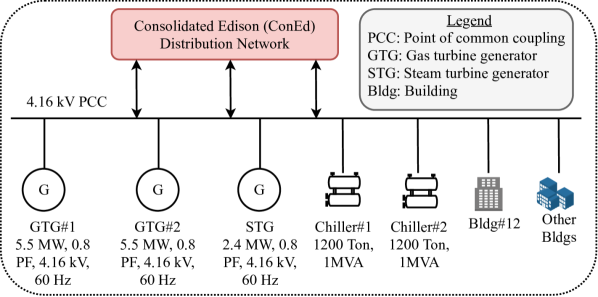
The case study uses the DR data for building #12 of New York University (NYU), which is a part of the NYU microgrid shown in Fig. 3 and is participating in the DR program organized by Consolidated Edison, the local electric power utility in NY [39, 40]. The aggregated DR of this building with over 20 DR events was randomized for 50 individual DR customers such that the power reduction of each DR customer is between kW- kW and the DR incentive is between $/kWh-2 $/kWh. The capacity and incentives observed during these 20 DR events are given as , }. The case study is carried out on a MacBook Air with a 2.2 GHz Intel Core i7 processor and 8 GB RAM. The non-convex and non-linear optimization in Eq. (8) is solved in Julia using Ipopt. All simulations instances described below were solved within one hour, which is sufficient to accommodate the time frame for DR event planning (e.g., Consolidated Edison sends their public, day-ahead advisory notice to DR customers 21 hours or more prior to a call window [41]).
IV-B Valuation of Historical Data
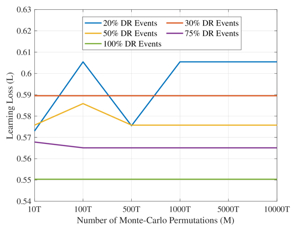
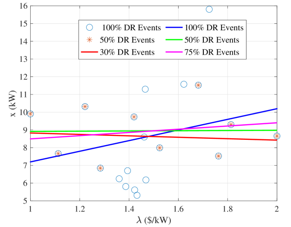
In this section, we investigate the effect of the number of historical DR events and DR customers on learning their behavior. First, we evaluate contributions of individual historical DR events towards learning the behavior of DR customers. Fig. 4 presents the MSE learning losses for the DR events of a randomly selected DR customer over randomly generated Monte-Carlo permutations. The learning loss in Fig. 4 is achieved in two steps. First, the contribution of each historical DR event in learning the behavior of each DR customer is ranked using the Shapely value theorem from Section III-D. That is, the greater the Shapley value of that DR event, the greater contribution it makes towards learning the actual value of . Second, all DR events are sorted in the order of their contribution and of the highest Shapley-valued DR events is used to compute the relative MSE learning loss. Since the calculation of Shapley value is a Monte-Carlo-based approximation, the learning losses of the DR events stabilize after Monte-Carlo permutations as shown in Fig. 4, where is the number of time instances with historical DR events. As Fig. 4 shows, the case when of the most Shapley-valued DR events is available for learning yields learning losses close to the case with availability of DR events. This means that the attacker can learn aggregated behavior of DR customers sufficiently well with only of DR events. Furthermore, Fig. 5 shows that the number of DR events available for the attack design does not significantly change the learned value of . Rather the contribution of the DR events in learning the behavior is significant. As a result, the Shapley value tends to be greater for DR events in the proximity of the curve learned from DR events. For example, this can be seen in Fig. 5, where 50% of the DR events with the greatest Shapley values are near the curve learned from DR events.
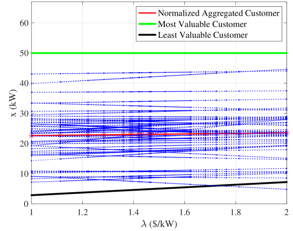
Next, we evaluate individual contributions of DR customers on learning their aggregated behavior. Fig. 6 presents the learned behavior of all DR customers and their aggregated behavior at DR event at time . The effect of each DR customer on the aggregated behavior is evaluated using Eq. (12). The aggregated behavior of the DR customers is normalized by to visualize their behaviors comparatively. The most valuable DR customer for attack design can be identified by the slope of its behavior (given by ), which aligns with the direction of the aggregated behavior. Conversely, the least valuable DR customer has its slope in the opposite direction. The intercept (given by ) of the most valuable DR customer is the largest among all DR customers and the least valuable DR customer has the smallest intercept. That is, the most and the least valuable customer has the greatest and lowest values of in Eq. (12). Therefore, in both offline and online attack cases, the attacker can rank compromised DR events and DR customers based on how critical they are for achieving a given objective of the planned attack and how much data is needed for an attack to succeed.
This relationship between DR customers/events data and their contribution towards the attack is established in a data-driven manner, rather than based on physical attributes (e.g., a type of DR appliances or an underlying energy conversion technology). As a result of the data-driven relationship, the valuation of DR customers/events is case-specific. Thus, drawing a physical intuition behind the physical attributes of the DR appliance and their Shapley value is not straightforward.
IV-C Attack Assessment
IV-C1 Monetary Attack
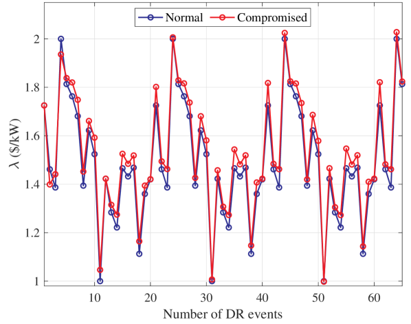
This section uses the most valued DR customers and DR events, obtained as described in Section IV-B, to launch a causative attack on the DR learning scheme described in Section III-C. Consider an attack that manipulates power curtailments of DR customers to increase DR incentives broadcasted for future DR events, thus making the DR program more costly for the utility/aggregator. To do so, the attacker sets as its objective in the optimization problem in Eq. (8). The decrease in is associated with a DR service that is more expensive to the aggregator and an increase in the incentive to the DR customers. Therefore, this attack can be launched by a customer or a group of customers (see Section III-B) to deliberately increase their DR incentives and, thus, payoffs. This increase in the DR incentive may not be economical for the aggregator/utility and, hence, may lead to a cancellation of the DR call. The attacker remains stealthy by delivering the committed DR capacity to the utility while manipulating the DR customers. At least DR events are needed before an aggregator learns the anomalous behavior of the DR customers (i.e., the target of is achieved within DR events). About of the DR customers with large Shapely values can achieve the attack objective in the DR events. Fig. 7 shows the DR incentives during normal and compromised states of DR customers. A considerable number of DR events is necessary for this attack to succeed. However, instead of acquiring a large number of DR events for attack planning, the attacker can operationalize an attack with fewer DR event observations, if the attacker does not seek to match the power curtailment and DR target amount as enforced in Eq. (8f). However, this mismatch observed in real-time by the aggregator/utility may inform them of the attack. Thus, the number of DR events required for attack success leads to a trade-off with attack stealthiness.
IV-C2 Technical Attack
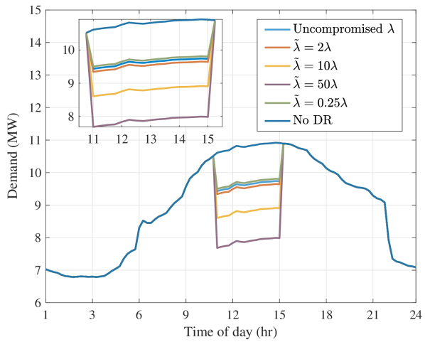
As opposed to the monetary attack described above, we shift in this section to technical attacks, which aim to instantly disrupt electricity supply. To illustrate this attack, we use the NYU microgrid described in Section IV-A. The NYU microgrid has a total generation capacity of 13.4 MW and is capable of islanding from the local distribution network operated by Consolidated Edison as described in [39]. We consider a DR event between 11:00 to 15:00 hours. The attacker manipulates a single value of broadcast by the utility/aggregator for that DR event by exploiting the devices and communication channel as shown in Fig. 2. Then, DR customers respond optimally to the compromised DR incentive as in Eq. (3). In turn, these responses of DR customers alter the demand of the microgrid during the DR event window. Fig. 8 demonstrates how this change in leads to changes in power curtailments of DR customers. If the attacker decreases by 4, the power curtailment is diminished by 3.8%. On the other hand, if the attacker increases by 50, the power curtailment of DR customers will increase by 21.5%. Both an unexpected increase and decrease in the demand of the microgrid leads to an under- or over-frequency event.
.
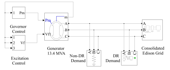
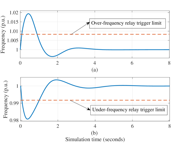
To demonstrate the frequency excursions in the NYU microgrid caused by the attacks, the NYU microgrid is modeled in MATLAB/Simulink as shown in Fig. 9. To make this model tractable, we aggregate three generators into one using an equivalent generator model with a speed governor controller and an excitation controller. The demand on the microgrid is divided into the DR and non-DR demands in these simulations. Since the attack with in Fig. 8 leads to the largest power curtailment (e.g., to 7.68 MW at 11:00 hours), we use it in the analysis. If the attack remains undetected, it incurs a sudden and significant demand increase at the DR end time (e.g., to 10.8 MW at 15:00 hours). These demand excursions, in turn, cause an over-frequency event of 1.018 per unit (p.u.) and an under-frequency event of 0.981 p.u. as shown in Figs. 10 (a,b) respectively. Since the attack creates sudden substantial changes in the microgrid demand at 11:00 and 15:00 hours, we simulate these two instances to observe the maximum possible frequency excursion in the microgrid. These frequency excursions can trigger the frequency relays, where the limits are set to 0.9916 p.u. and 1.0083 p.u. for under- and events over-frequency as recommended by IEEE Standard 1547 [42]. Depending on the range, in which the settings of the under- and over frequency relays can be adjusted, these frequency excursions may island the microgrid from the Consolidated Edison network and trip the microgrid generators. Such excursions can also cause wear and tear on the microgrid components and may propagate into the systems.
V Defending the Attack
The success of the causative attack mechanism described in this paper hinges on the ability of the attacker to tamper with data on DR incentives and power curtailments. This data can be infiltrated at various devices and communication channels between DR customers and the utility/aggregator. The use of industry-grade security techniques on DRAS servers and communication channels, e.g., OpenADR, BACnet, CTA-2045, and increased awareness of cyber hygiene among DR customers can reduce the likelihood of intrusion. In contrast, idiosyncratic cyber hygiene of DR customers and various possibilities of zero-day vulnerabilities provide additional entry points for attackers. Therefore, defense schemes against such causative attacks are needed to secure ML applications for DR programs. There are several such defense schemes in recent ML security literature [43, 44]. Steinhardt et al. [43] proposed a defense mechanism that aims to remove the compromised data from the original dataset. This data sanitizing process is achieved by estimating the probability distribution of the uncompromised dataset in the attacked dataset. Similarly, Zhang and Zhu [44] presented a game-theoretic defense scheme based on a distributed support vector machine, where the defender does not update the algorithm if the compromised data samples are detected. However, performance of these security mechanisms varies when applied to a specific engineering domains and to the best of the authors’ knowledge there is no such mechanism designed for DR programs.
VI Conclusion
This paper presents a novel attack on the ADR learning used by an utility/aggregator by either providing an erroneous response from the DR customers or by broadcasting anomalous incentives to the DR customers. This causative attack is launched on the ADR framework of an utility/aggregator by learning the quadratic cost function of the DR customers and broadcasting an optimal DR incentive to the customers. As shown, the attack can be launched on the data synthesized from a DR-enrolled building. Such causative attacks on the learning schemes used by utilities/aggregators are realistic especially when there are a larger number of DR events.
References
- [1] M. Surampudy, B. Chew, M. Keller, and T. Gibson, “2019 utility demand response market snapshot,” Smart Electric Power Alliance, Washington, DC, USA, 2019. [Online]. Available: https://sepapower.org/resource/2019-utility-demand-response-market-snapshot/
- [2] California Public Utilities Commission. ”Consumer FAQ on DR Providers (also known as Aggregators),” Accessed May 6, 2020. [Online]. Available: https://www.cpuc.ca.gov/General.aspx?id=6306
- [3] PG&E. ”Third-party Demand Response Provider or Aggregator,” Accessed June 16, 2020. [Online]. Available: https://www.pge.com/en_US/small-medium-business/save-energy-and-money/rebates-and-incentives/energy-management-incentives/rule-24/third-party.page
- [4] OpenADR Alliance. Accessed June 1, 2020. [Online]. Available: https://www.openadr.org
- [5] J. Qi, Y. Kim, C. Chen, X. Lu, and J. Wang, “Demand response and smart buildings: A survey of control, communication, and cyber-physical security,” ACM Transactions on Cyber-Physical Systems, vol. 1, no. 4, pp. 1–25, 2017.
- [6] K. Mahmood, S. A. Chaudhry, H. Naqvi, T. Shon, and H. F. Ahmad, “A lightweight message authentication scheme for smart grid communications in power sector,” Computers & Electrical Engineering, vol. 52, pp. 114–124, 2016.
- [7] AlphaGuardian. ”California’s SB327 and IIoT Cybersecurity,” Accessed June 16, 2020. [Online]. Available: https://www.alphaguardian.net/category/demand-response-vulnerabilities/
- [8] M. Kumar, “How to Hack WiFi Password Easily Using New Attack On WPA/WPA2,” The Hacker News, Nov. 25, 2018. [Online]. [Online]. Available: https://thehackernews.com/2018/08/how-to-hack-wifi-password.html
- [9] X. Fan, F. Susan, W. Long, and S. Li, “Security analysis of zigbee,” Comput. Netw. Secur. Class, Massachusetts Inst. Technol., Cambridge, MA, USA, Rep, 2017.
- [10] M. Seijo Simó, G. López López, and J. I. Moreno Novella, “Cybersecurity vulnerability analysis of the PLC PRIME standard,” Security and Communication Networks, vol. 2017, 2017.
- [11] K. Weaver and S. Solutions, “Smart meter deployments result in a cyber attack surface of “unprecedented scale,”,” Smart Grid Awareness, 2017.
- [12] G. Carracedo, “Smart Meters A proof of concept: hacking a smart meter,” TARLOGIC, Mar. 6, 2020. [Online]. Available: https://www.tarlogic.com/en/blog/smart-meters-a-proof-of-concept-hacking-a-smart-meter/
- [13] S. Kumar, H. Kumar, and G. R. Gunnam, “Security integrity of data collection from smart electric meter under a cyber attack,” in 2019 2nd International Conference on Data Intelligence and Security (ICDIS). IEEE, 2019, pp. 9–13.
- [14] F. M. Tabrizi and K. Pattabiraman, “Design-level and code-level security analysis of IoT devices,” ACM Transactions on Embedded Computing Systems (TECS), vol. 18, no. 3, pp. 1–25, 2019.
- [15] S. Acharya, Y. Dvorkin, H. Pandžić, and R. Karri, “Cybersecurity of smart electric vehicle charging: A power grid perspective,” IEEE Access, vol. 8, pp. 214 434–214 453, 2020.
- [16] B. Thomas, “FBI Alerts Companies of Cyber Attacks Aimed at Supply Chains,” BITSIGHT, Feb. 21, 2020. [Online]. Available: https://www.bitsight.com/blog/fbi-alerts-companies-of-cyber-attacks-supply-chains
- [17] S. Acharya, Y. Dvorkin, and R. Karri, “Public plug-in electric vehicles + grid data: Is a new cyberattack vector viable?” IEEE Transactions on Smart Grid, pp. 1–1, 2020.
- [18] S. Soltan, P. Mittal, and H. V. Poor, “Blackiot: IoT botnet of high wattage devices can disrupt the power grid,” in 27th USENIX Security Symposium (USENIX Security 18), 2018, pp. 15–32.
- [19] S. Amini, F. Pasqualetti, M. Abbaszadeh, and H. Mohsenian-Rad, “Hierarchical location identification of destabilizing faults and attacks in power systems: A frequency-domain approach,” IEEE Transactions on Smart Grid, vol. 10, no. 2, pp. 2036–2045, March 2019.
- [20] G. Raman, J. C. Peng, and T. Rahwan, “Manipulating residents’ behavior to attack the urban power distribution system,” IEEE Transactions on Industrial Informatics, vol. 15, no. 10, pp. 5575–5587, 2019.
- [21] K. Khezeli and E. Bitar, “Risk-sensitive learning and pricing for demand response,” IEEE Transactions on Smart Grid, vol. 9, no. 6, pp. 6000–6007, 2017.
- [22] P. Li, H. Wang, and B. Zhang, “A distributed online pricing strategy for demand response programs,” IEEE Transactions on Smart Grid, vol. 10, no. 1, pp. 350–360, 2017.
- [23] R. Mieth and Y. Dvorkin, “Online learning for network constrained demand response pricing in distribution systems,” IEEE Transactions on Smart Grid, vol. 11, no. 3, pp. 2563–2575, 2020.
- [24] N. Tucker, A. Moradipari, and M. Alizadeh, “Constrained thompson sampling for real-time electricity pricing with grid reliability constraints,” IEEE Transactions on Smart Grid, pp. 1–1, 2020.
- [25] G. Feller, “AI And Machine Learning for Better Energy Demand Response,” T&D World, May 13, 2019. [Online]. Available: https://www.tdworld.com/distributed-energy-resources/demand-side-management/article/20972576/ai-and-machine-learning-for-better-energy-demand-response
- [26] S. Mei and X. Zhu, “Using machine teaching to identify optimal training-set attacks on machine learners,” in Twenty-Ninth AAAI Conference on Artificial Intelligence, 2015.
- [27] W. Liu, B. Dai, A. Humayun, C. Tay, C. Yu, L. B. Smith, J. M. Rehg, and L. Song, “Iterative machine teaching,” in Proceedings of the 34th International Conference on Machine Learning-Volume 70. JMLR. org, 2017, pp. 2149–2158.
- [28] L. S. Shapley, “A value for n-person games,” Contributions to the Theory of Games, vol. 2, no. 28, pp. 307–317, 1953.
- [29] J. Castro, D. Gómez, and J. Tejada, “Polynomial calculation of the shapley value based on sampling,” Computers & Operations Research, vol. 36, no. 5, pp. 1726–1730, 2009.
- [30] R. Jia, D. Dao, B. Wang, F. A. Hubis, N. Hynes, N. M. Gürel, B. Li, C. Zhang, D. Song, and C. J. Spanos, “Towards efficient data valuation based on the shapley value,” in The 22nd International Conference on Artificial Intelligence and Statistics. PMLR, 2019, pp. 1167–1176.
- [31] A. Ghorbani and J. Zou, “Data shapley: Equitable valuation of data for machine learning,” in International Conference on Machine Learning. PMLR, 2019, pp. 2242–2251.
- [32] S. Burger, J. P. Chaves-Ávila, C. Batlle, and I. J. Pérez-Arriaga, “A review of the value of aggregators in electricity systems,” Renewable and Sustainable Energy Reviews, vol. 77, pp. 395–405, 2017.
- [33] R. Mieth, S. Acharya, A. Hassan, and Y. Dvorkin, “Learning-enabled residential demand response: Automation and security of cyberphysical demand response systems,” IEEE Electrification Magazine, vol. 9, no. 1, pp. 36–44, 2021.
- [34] P. Samadi, H. Mohsenian-Rad, R. Schober, and V. W. Wong, “Advanced demand side management for the future smart grid using mechanism design,” IEEE Transactions on Smart Grid, vol. 3, no. 3, pp. 1170–1180, 2012.
- [35] A. M. Radoszynski, V. Dvorkin, and P. Pinson, “Accommodating bounded rationality in pricing demand response,” in 2019 IEEE Milan PowerTech, 2019, pp. 1–6.
- [36] J. L. Mathieu, D. S. Callaway, and S. Kiliccote, “Examining uncertainty in demand response baseline models and variability in automated responses to dynamic pricing,” in IEEE European Control Conference, 2011, pp. 4332–4339.
- [37] N. Li, L. Chen, and S. H. Low, “Optimal demand response based on utility maximization in power networks,” in 2011 IEEE power and energy society general meeting. IEEE, 2011, pp. 1–8.
- [38] ISO New England. ”Demand-Response Threshold Price Details,” Accessed June 16, 2020. [Online]. Available: https://www.iso-ne.com/isoexpress/web/reports/pricing/-/tree/demand-response-threshold-price-details
- [39] A. Hassan, S. Acharya, M. Chertkov, D. Deka, and Y. Dvorkin, “A hierarchical approach to multienergy demand response: From electricity to multienergy applications,” Proceedings of the IEEE, vol. 108, no. 9, pp. 1457–1474, 2020.
- [40] Con Edison. ”Smart AC,” Accessed Mar. 7, 2020. [Online]. Available: https://www.coned.com/en/save-money/rebates-incentives-tax-credits/rebates-incentives-tax-credits-for-residential-customers/smart-air-conditioners
- [41] ConEdison. ”Commercial Demand Response (Rider T) Program Guidelines,” Mar. 1, 2021. [Online]. Available: https://www.coned.com/-/media/files/coned/documents/save-energy-money/rebates-incentives-tax-credits/smart-usage-rewards/smart-usage-program-guidelines.pdf?la=en
- [42] “IEEE standard for interconnecting distributed resources with electric power systems - amendment 1,” IEEE Std 1547a-2014 (Amendment to IEEE Std 1547-2003), pp. 1–16, 2014.
- [43] J. Steinhardt, P. W. W. Koh, and P. S. Liang, “Certified defenses for data poisoning attacks,” in Advances in neural information processing systems, 2017, pp. 3517–3529.
- [44] R. Zhang and Q. Zhu, “A game-theoretic defense against data poisoning attacks in distributed support vector machines,” in 2017 IEEE 56th Annual Conference on Decision and Control (CDC). IEEE, 2017, pp. 4582–4587.