Deflection and Gravitational Lensing in Kerr spacetime off equatorial plane

Abstract

This paper investigates the off-equatorial plane deflection and gravitational lensing of both null and timeline signals in Kerr spacetime in the weak deflection limit, with the finite distance effect of the source and detector taken into account. The deflection in both the Boyer-Linquidist $\phi$ and $\theta$ directions are computed as power series of $M/r_{0}$ and $r_{0}/r_{s,d}$, where $M,~{}r_{s,d}$ are the spacetime mass and source and detector radius respectively, and $r_{0}$ is the minimal radius of the trajectory. The coefficients of these series are simple trigonometric functions of $\theta_{\text{e}}$, the extreme value of $\theta$ coordinate of the trajectory. A set of exact gravitational lensing equations is used to solve $r_{0},~{}\theta_{\text{e}}$ for a given deflection $\delta\theta$ and $\delta\phi$ of the source, and two images are always obtained. The apparent angles and their magnifications of these images are solved and their dependence on various parameters, especially spacetime spin $\hat{a}$ are analyzed in great detail. It is found that generally there exist two critical spacetime spin which separate the signals reaching the detector from different sides of the spin axis and the images to appear either in the first or the second, and the third and the fourth quadrant of the celestial plane. Three potential applications of these results are discussed.

I Introduction

Deflection and gravitational lensing of lightrays are fundamental features of signals’ motion in curved spacetimes. The early confirmation of the former established general relativity (GR) as a more accurate description of gravity [23]. The GL has become a very important tool in astronomy, from measuring the lens mass and mass distribution [22] to study the property of dark mass and energy [20, 21]. With the advancement of modern observation technology, especially the fast development of black hole (BH) observations [24, 25] , the physics of bending and GL of signals in the strong deflection limit (SDL) has become essential for the correct understanding of the relevant observation results.

Theoretically, the deflection and GL of signals are most easily understood and thoroughly studied in static and spherically symmetric (SSS) spacetimes, or in the equatorial plane of stationary and axisymmetric (SAS) spacetimes. Different techniques, such as the Gauss-Bonnet theorem-based geometrical method [18, 19] and perturbative methods [26, 41, 46], have been used to study deflections of not only null but timeline signals. Various effects, such as the finite distance effect of the source and detectors [9, 10, 11], as well as those of the spacetime parameters (spin, charges [16], magnetic field [14] etc.) and signal properties (spin [15] and charge [12, 45]), have been extensively investigated in recent years. Observationally, however Kerr BH is still the most simple and natural BH considered by astronomers [24, 25], and even the Kerr-Newmann (KN) spacetime is not as popular due to its nonzero charge.

The signal deflection and GL of lightrays in Kerr spacetime have also been intensively studied. Although relevant numerical packages can often yield the general motions in Kerr spacetime [17], analytical works about the deflection and GL in Kerr (or KN) spacetime are more concentrated on the motion in the (quasi-)equatorial plane [33, 31, 32, 34, 35, 29, 26, 30]. For analytical works dealing with non-equatorial plane motions in the Kerr spacetime, AAA studied the Wilkins investigated the frequencies of the bound orbit in both the $\theta$ and $\phi$ directions [28]. Fujita and Hikida studied the bound timeline orbit solution in terms of Mino time [27]. Hackmann and Xu classified motions of test particles in Kerr and KN spacetimes [40, 44]. For works most relevant to the present paper, Bray calculated the deflection angles of null rays in Kerr spacetime in terms of the conserved constant of the motion [42]. Sereno and De Luca updated this work and solve the image positions using some approximate geometrical relations [36]. Kraniotis found image locations for observers with particular latitudes [43].

The above works however did not systematically takes into account the finite distance effect of the source and observer. The lens equations used were also based on the first order approximation of the geometrical relations linking the angles of the source with and without the lens. In this work, we will develop a perturbative method that can compute the deflection and GL for arbitrary orientation directions of the Kerr spacetime spin. Moreover, the method can take into account the finite distance effect of the source and observer, which allows us to use exact GL equations to obtain the image positions, their magnifications and time delays. Furthermore, we will not limit the trajectories to that of lightrays but deal with signals with general asymptotic velocity, including both null and timeline ones. The deflection and GL of timeline signals have drawn more attention in recent years [16, 10, 41, 46] with the fast development of neutrino [6, 7, 2] and cosmic ray (see [13] and references therein) observation technologies, and the discovery of gravitational waves (GW) and the fact that GWs in some beyond GR theories are massive [1, 3].

In this work, we will show that the deflection angles in Kerr spacetime with mass $M$ in the weak deflection limit (WDL) in both the $\phi$ and $\theta$ directions can be expressed in quasi-power series forms of $M/r_{0}$ and $r_{0}/r_{s,d}$ where $r_{0},~{}r_{s,d}$ are the minimal radius of the trajectory and the source and detector radii. The coefficients of these series are functions of $\hat{a}$, the spin angular momentum per unit mass, and $v$ (or $E$), the asymptotic velocity of the signal. After solving a set of exact GL equations, we will determine the image positions and magnifications of a source that has small deflections $\delta\theta$ and $\delta\phi$. The dependence of these quantities, as well as the time delay between images, on the spacetime spin size and its orientation and other parameters will be shown explicitly. We also used these results to discuss some potential applications in astronomical observations.

The work is organized as follows. In Sec. II we introduce the basic setup of the problem. In Sec. III we develop the perturbative method, using which we express the deflections as power series. The GL equations are solved in Sec. IV to obtain the image locations, magnifications and time delays. The effects of various parameters on them are also investigated. Sec. A discusses a few potential applications of the results and concludes the paper. Throughout the work, we use the natural units $G=c=1$.

II Preliminaries

The Kerr spacetime with the Boyer-Lindquist coordinates $(t,r,\theta,\phi)$ can be described by the following metric

$$\mathrm{d}s^{2}= -\frac{\Delta}{\Sigma}\left(\mathrm{d}t-a\sin^{2}\theta\mathrm{d}\phi\right)^{2}+\frac{\Sigma}{\Delta}\mathrm{d}r^{2}+\Sigma\mathrm{d}\theta^{2}$$

$$+\frac{\sin^{2}\theta}{\Sigma}\left[\left(r^{2}+a^{2}\right)\mathrm{d}\phi-a\mathrm{d}t\right]^{2}$$ (1)

where

$$\Delta(r)=r^{2}-2Mr+a^{2}$$ (2)

$$\Sigma(r,\theta)=r^{2}+a^{2}\cos^{2}\theta$$ (3)

and $a=J/M$ is the angular momentum per unit mass of the central BH, with $M$ being its total mass. The motion of test particles in this spacetime is governed by the geodesic equation

$$\frac{\mathrm{d}^{2}x^{\rho}}{\mathrm{d}\sigma^{2}}+\Gamma_{\mu,\nu}^{\rho}\frac{\mathrm{d}x^{\mu}}{\mathrm{d}\sigma}\frac{dx^{\nu}}{d\sigma}=0$$ (4)

where $\sigma$ is the proper time of timelike particles or affine parameter of null signals. Using the metric (1), this becomes after the first integrals [39]

$$\Sigma^{2}\left(\frac{\mathrm{d}r}{\mathrm{d}\sigma}\right)^{2}=R(r)$$ (5)

$$\Sigma^{2}\left(\frac{\mathrm{d}\cos\theta}{\mathrm{d}\sigma}\right)^{2}=\Theta(\cos\theta)$$ (6)

$$\Sigma\frac{\mathrm{d}\phi}{\mathrm{d}\sigma}=\frac{2aMrE-a^{2}L}{\Delta}+L\csc^{2}\theta$$ (7)

$$\Sigma\frac{\mathrm{d}t}{\mathrm{d}\sigma}=\frac{r^{2}+a^{2}}{\Delta}\left[E\left(r^{2}+a^{2}\right)-aL\right]+a\left(L-aE\sin^{2}\theta\right)$$ (8)

$$\Sigma\frac{\mathrm{d}t}{\mathrm{d}\sigma}=\frac{E(r^{2}+a^{2})^{2}-2aLMr}{\Delta}-Ea^{2}\sin^{2}\theta$$ (9)

where

$$R(r)= \left[E\left(r^{2}+a^{2}\right)-aL\right]^{2}-\Delta\left(K+m^{2}r^{2}\right)$$ (10)

$$\Theta(\cos\theta)= \left(1-\cos^{2}\theta\right)\left[K-a^{2}m^{2}\cos^{2}\theta+2LaE\right.$$

$$\left.-a^{2}E^{2}\left(1-\cos^{2}\theta\right)\right]-L^{2}$$ (11)

and $m,~{}E,~{}L,~{}K$ are respectively the mass, the conserved energy and angular momentum per unit mass of the signal, and the Carter constant.

In asymptotically flat spacetimes that we focus on, $E$ is related to the velocity $v$ by

$$E=\frac{m}{\sqrt{1-v^{2}}}$$ (12)

One of the main motivations of the work is to obtain the deflection of the signals that are not restricted to the equatorial plane. For this purpose, using Eqs. (5) and (6), we first get

$$\frac{s_{r}\mathrm{d}r}{\sqrt{R(r)}}=\frac{s_{\theta}\mathrm{d}\cos\theta}{\sqrt{\Theta(\cos\theta)}}$$ (13)

Here the $s_{\theta}$ and $s_{r}$ are two signs introduced when taking the square root in Eqs. (5) and (6) respectively. Using Eqs. (5) and (13) respectively in the first and last terms in the right-hand side of Eq. (7), we obtain

$$\mathrm{d}\phi= \frac{2aMrE-a^{2}L}{\Delta}\frac{s_{r}\mathrm{d}r}{\sqrt{R(r)}}+\frac{L}{1-\cos^{2}\theta}\frac{s_{\theta}\mathrm{d}\cos\theta}{\sqrt{\Theta(\cos\theta)}}$$ (14)

When proper initial conditions are given, integrating Eqs. (13) and (14) from the source located at radius $r_{s}$ to the detector at radius $r_{d}$ will yield both the deflection $\Delta\phi$ and $\Delta\theta$ in the $\phi$ and $\theta$ coordinates respectively. If we let $r_{s}$ (or $r_{d}$) vary, then knowing the integral results of Eqs. (13) and (14) is equivalent to the knowledge of the solutions $\phi(r)$ and $\theta(r)$.

Before carrying on more detailed computation however, there are a few comments that we should make regarding these equations and their integrals. The first is to note that according to Ref. [40], there are quite a few kinds of motion in the Kerr spacetime when the particle is not limited to the equatorial plane. The kind we will study is classified as the IVb case, which is a flyby orbit, in other words, the particle will have come from a spacial infinity to reach a periapsis and then return to spacial infinity. In this case, we can adjust the orbit parameters so that the periapsis is far from the event horizon and therefore the deflection of the signal is generally weak, which will allow us to carry out a weak field perturbative study. In this limit, we can safely assume that the $\theta$ coordinate will only experience one local extreme along the entire trajectory. We denote this extreme value as $\theta_{\text{e}}$. If the signal flies by the central BH from above (or below) the equatorial plane, $\theta_{\text{e}}$ will be a minimum (or maximum), while $\cos\theta_{\text{e}}$ will be a local maximum (or minimum).

With the above consideration, we can integrate Eqs. (13) and (14) from the source located at $(r_{s},~{}\theta_{s},~{}\phi_{s})$ to the detector at $(r_{d},~{}\theta_{d},~{}\phi_{d})$ to obtain the following relation

$$\left(\int_{r_{0}}^{r_{s}}+\int_{r_{0}}^{r_{d}}\right)\frac{\mathrm{d}r}{\sqrt{R(r)}}=\left(\int_{\theta_{s}}^{\theta_{\text{e}}}+\int_{\theta_{d}}^{\theta_{\text{e}}}\right)\frac{s_{r\theta}\mathrm{d}\cos\theta}{\sqrt{\Theta(\cos\theta)}}$$ (15)

$$s_{l}\int_{\phi_{s}}^{\phi_{d}}\mathrm{d}\phi=\left(\int_{r_{0}}^{r_{s}}+\int_{r_{0}}^{r_{d}}\right)\frac{2aMrE-a^{2}L}{\Delta\sqrt{R(r)}}\mathrm{d}r$$

$$+\left(\int_{\cos\theta_{s}}^{\cos\theta_{\text{e}}}+\int_{\cos\theta_{d}}^{\cos\theta_{\text{e}}}\right)\frac{s_{r\theta}L}{1-\cos^{2}\theta}\frac{\mathrm{d}\cos\theta}{\sqrt{\Theta(\cos\theta)}}$$ (16)

Here $r_{0}$ is the minimum radius along the trajectory, and $\theta_{\text{e}}$ is the extreme value of the $\theta$ coordinate. $s_{r\theta}=\pm 1$ and $s_{l}=\pm 1$ are the signs induced from Eqs. (13) and (14) when carrying out the integrals. Here $s_{l}$ is the same as the sign of the orbital angular momentum introduced in Eq. (19). $r_{0}$ and $\theta_{\text{e}}$ can be related to the conserved constants $L,~{}K$ and $E$ through their definitions

$$\left.\frac{\mathrm{d}r}{\mathrm{d}\sigma}\right|_{r=r_{0}}=0,~{}~{}\left.\frac{\mathrm{d}\cos\theta}{\mathrm{d}\sigma}\right|_{\theta=\theta_{\mathrm{e}}}=0.$$ (17)

From Eqs. (5) and (6), we see that the above equation is equivalent to finding the root of the right-hand sides of Eqs. (10) and (11) equal to zero. Using these, we have obtained the analytical expression of $\theta_{\text{e}}$ in terms of $L,~{}K$ and $E$

$$\cos^{2}\theta_{e}=\frac{1}{2a^{2}\left(E^{2}-m^{2}\right)}\left\{a^{2}\left(2E^{2}-m^{2}\right)-2aEL-K\right.{}$$

$$+\left\{(a^{2}m^{2}-K)^{2}+4aL\left[EK-a(aE-L)m^{2}\right]\right\}^{1/2}\}$$ (18)

$r_{0}$ is a root of order four polynomial equations and too lengthy to show here. Here we also show the simpler formulas of $L$ and $K$ in terms of $r_{0},~{}\theta_{\text{e}}$ and $E$

$$L= \frac{s_{l}\sin\theta_{\mathrm{e}}\chi-2aE\sin^{2}\theta_{\mathrm{e}}Mr_{0}}{\Sigma(r_{0},\theta_{\mathrm{e}})-2Mr_{0}},$$ (19)

$$K= a^{2}m^{2}\cos^{2}\theta_{\mathrm{e}}+(L\csc\theta_{\mathrm{e}}-aE\sin\theta_{\mathrm{e}})^{2}$$ (20)

where

$$\chi=\sqrt{\Sigma(r_{0},\theta_{\mathrm{e}})\Delta(r_{0})\left[\Sigma(r_{0},\theta_{\mathrm{e}})(E^{2}-m^{2})+2Mm^{2}r_{0}\right]}{}$$

and the $s_{l}$ in front of $\chi$ is valid in the weak deflection limit. These relations can be used to replace the $L$ and $K$ in the integrals (15) and (16) when we carry out these integrations later.

Among the six coordinates $(r_{s},\theta_{s},\phi_{s})$ and $(r_{d},\theta_{d},\phi_{d})$, we will assume that the $r_{s},~{}r_{d}$ and $\theta_{s}$ are known. The $\phi_{s}$ and $\phi_{d}$ are unnecessary to know a priori and indeed $\Delta\phi\equiv\phi_{d}-\phi_{s}$ is the deflection angle we desire to solve. We also note that the integral in Eq. (16) is exactly the deflection $\Delta\phi$ in the $\phi$ direction. For the deflection $\Delta\theta\equiv\theta_{d}+\theta_{s}-\pi$ in the $\theta$ direction, we see from Eq. (15) that once $r_{s},~{}r_{d}$ and $\theta_{s}$ are given, and if one can carry out the integral in this equation, then solving the resultant algebraic equation will allow us to determine $\theta_{d}$ and consequently $\Delta\theta$.

One of the main efforts of this work is to find proper, tractable ways to carry out these integrals. We will show in the next section that there exists a perturbative method to systematically approximate these deflections, and the result takes a series form of ***.

III Perturbative method and results

III.1 Perturbative expansion method

The key to carry out the integrations of Eqs. (15) and (16) is to find a proper way to expand the integrands, after which the integral can always be carried out to any desired accuracy. The weak deflection assumption provides a natural choice of such an expansion parameter, that is, the ratio $M/r_{0}$ between the source mass and the closest radius. Before carrying out the expansion however, it is important to note that the orbital angular momentum $L$ or the Cater constant $K$ of the signal are not easily measurable, while $E$ is either not relevant for null signal or can be easily locally measured for timelike signals. Therefore one just has to replace $L$ and $K$ in Eqs. (15) and (16) by Eqs. (19) and (20). For simpler notations, introducing the new integration variables, $p\equiv r_{0}/r$ and $c\equiv\cos\theta$, as well as the auxiliary notations

$$p_{s,d} =r_{0}/r_{s,d},~{}c_{s,d,\text{e}}=\cos\theta_{s,d.\text{e}},{}$$

$$~{}s_{s,d,\text{e}} =\sin\theta_{s,d,\text{e}},~{}t_{s,d,\text{e}}=\tan\theta_{s,d,\text{e}},$$ (21)

and then carrying out the expansions using $M/r_{0}$ as a small parameter, Eqs. (15) and (16) become

$$\left(\int_{1}^{p_{s}}+\int_{1}^{p_{d}}\right)\sum_{i=1}^{\infty}\frac{f_{r,i}(p)}{(1+p)^{i-1}\sqrt{1-p^{2}}}\left(\frac{M}{r_{0}}\right)^{i}\mathrm{d}p$$

$$=\left(\int_{c_{s}}^{c_{\text{e}}}+\int_{c_{d}}^{c_{\text{e}}}\right)\sum_{i=1}^{\infty}\frac{f_{\theta,i}(c)}{\sqrt{c_{\text{e}}^{2}-c^{2}}}\left(\frac{M}{r_{0}}\right)^{i}\mathrm{d}c,$$ (22)

$$\Delta\phi= \left(\int_{1}^{p_{s}}+\int_{1}^{p_{d}}\right)\sum_{i=2}^{\infty}\frac{g_{r,i}(p)}{(1+p)^{i-2}\sqrt{1-p^{2}}}\left(\frac{M}{r_{0}}\right)^{i}\mathrm{d}p$$

$$+\left(\int_{c_{s}}^{c_{\text{e}}}+\int_{c_{d}}^{c_{\text{e}}}\right)\sum_{i=0}^{\infty}\frac{s_{r\theta}g_{\theta,i}(c)s_{\text{e}}}{\sqrt{c_{\text{e}}^{2}-c^{2}}}\left(\frac{M}{r_{0}}\right)^{i}\mathrm{d}c$$ (23)

where $f_{r,i},~{}f_{\theta,i},~{}g_{r,i},~{}g_{\theta,i}$ are the Taylor expansion coefficients whose exact forms can be worked out easily. Here we show the first few orders of them

$$f_{r,1}= \frac{1}{MvE},~{}f_{r,2}=\frac{p(1-(1+p)v^{2})}{Mv^{3}E},~{}\cdots,$$ (24a)

$$f_{\theta,1}= \frac{1}{MvE},~{}f_{\theta,2}=-\frac{1}{Mv^{3}E},~{}\cdots,$$ (24b)

$$g_{r,2}= \hat{a}p\left(-\frac{2s_{l}}{v}+\hat{a}s_{\text{e}}p\right),~{}\cdots,$$ (24c)

$$g_{\theta,0}= \frac{1}{1-c^{2}},~{}g_{\theta,1}=0,~{}g_{\theta,2}=\frac{\hat{a}^{2}}{2},~{}\cdots,$$ (24d)

where $\hat{a}\equiv a/M$ and the higher order coefficients are too lengthy to show here.

Since all $f_{r,i}$ and $g_{r,i}$ are polynomials of $p$ and $f_{\theta,i}$ and $g_{\theta,i}~{}(i>0)$ are polynomials of $c^{2}$, then the integrability of expansions in Eqs. (22) and (23) relies on the integrability of the following integrals

$$\int_{1}^{p_{s,d}}\frac{\mathrm{polynomial}(p)}{(1+p)^{i-1}\sqrt{1-p^{2}}}\mathrm{d}p~{}~{}(i\geq 1),$$ (25)

$$\int_{c_{s,d}}^{c_{\text{e}}}\frac{\mathrm{polynomial}(c^{2})}{\sqrt{c_{\text{e}}^{2}-c^{2}}}\mathrm{d}c.$$ (26)

Fortunately, the above forms are always integrable (see Appendix A for the proof) and therefore this guarantees that we can obtain a series solution of the deflection angles.

After integration, the results for Eqs. (22) and (23) then become

$$\sum_{j=s,d}\sum_{i=1}^{\infty}F_{r,i}(p_{j})\left(\frac{M}{r_{0}}\right)^{i}=\sum_{j=s,d}\sum_{i=1}^{\infty}F_{\theta,i}(c_{j},c_{\text{e}})\left(\frac{M}{r_{0}}\right)^{i},$$ (27)

$$\Delta\phi=\sum_{j=s,d}\left[\sum_{i=2}^{\infty}G_{r,i}(p_{j})+\sum_{i=0}^{\infty}G_{\theta,i}(c_{j},c_{\text{e}})\right]\left(\frac{M}{r_{0}}\right)^{i}.$$ (28)

Here the coefficient functions $F_{r,i},~{}F_{\theta,i},~{}G_{r,i},~{}G_{\theta,i}$ of the series of $(M/r0)$ are results of integrations of terms containing corresponding $f_{r,i},~{}f_{\theta,i},~{}g_{r,i},~{}g_{\theta,i}$, and therefore are also functions of the corresponding integration limits. The first few of them, for $j=s$ or $d$, are

$$F_{r,1}= \frac{1}{MvE}\left[\frac{\pi}{2}-\sin^{-1}({p_{j}})\right],$$ (29a)

$$F_{r,2}= \frac{1}{Ev^{3}M}\left[\sqrt{1-{p_{j}}^{2}}\left(\frac{1}{1+{p_{j}}}+v^{2}\right)+\sin^{-1}({p_{j}})-\frac{\pi}{2}\right],$$ (29b)

$$F_{\theta,1}= \frac{1}{MvE}\left(\frac{\pi}{2}-\sin^{-1}\left(\frac{c_{j}}{c_{\text{e}}}\right)\right),$$ (29c)

$$F_{\theta,2}= \frac{1}{MvE}\left(\sin^{-1}\left(\frac{{c_{j}}}{c_{\text{e}}}\right)-\frac{\pi}{2}\right),$$ (29d)

$$G_{r,2}= \frac{2\hat{a}s_{l}}{v}\sqrt{1-p_{i}^{2}}-\frac{1}{2}\hat{a}^{2}s_{\text{e}}\left[p_{i}\sqrt{1-p_{i}^{2}}+\cos^{-1}(p_{i})\right]$$ (29e)

$$G_{\theta,0}= \frac{\pi}{2}-s_{r\theta}\tan^{-1}\left(\frac{c_{j}s_{\text{e}}}{\sqrt{c_{\text{e}}^{2}-c_{j}^{2}}}\right),$$ (29f)

$$G_{\theta,1}= 0,$$ (29g)

$$G_{\theta,2}= \frac{1}{4}\hat{a}^{2}s_{\text{e}}\left(\pi-s_{r\theta}2\sin^{-1}\left(\frac{c_{j}}{c_{\text{e}}}\right)\right)$$ (29h)

One has to be careful when interpreting the Eqs. (27) and (28). Although Eq. (28) looks like a series of $(M/r_{0})$ with $G_{r,i}$ and $G_{\theta,i}$ as coefficients for the deflection $\Delta\phi$, it is still not the true final perturbative series of $(M/r_{0})$ comparable with computations in the equatorial plane. Reason one is that there exists dependence of $p_{s,d}$ on $r_{0}$ (see Eq. (21)). The second and deeper reason is that, as we pointed out before this section, among the parameters $r_{s,d},~{}\theta_{s,d},~{}r_{0}$ and $\theta_{\text{e}}$, not all of them are independent. Indeed, $\theta_{d}$ can be related to other parameters, particularly $r_{0}$, and this has to be taken into account when attempting to obtain a $(M/r_{0})$ series of $\Delta\phi$. This relation can be derived from Eq. (27) using two methods, the perturbative method and Jacobi elliptic function method respectively. Here will directly present the result of this relation but postpone its derivation to Appendix B

$$c_{d}\equiv\cos\theta_{d}=\sum^{\infty}_{i=0}h_{i}\left(\frac{M}{r_{0}}\right)^{i}$$ (30)

where

$$h_{0}= c_{\text{e}}\cos a_{1}$$ (31)

$$h_{1}= -\frac{c_{\text{e}}}{v^{2}}a_{2}\sin a_{1}$$ (32)

$$h_{2}= -\frac{c_{\text{e}}}{4}\left[a_{3}\sin a_{1}+\cos a_{1}\left(\frac{2}{v^{4}}a_{2}^{2}+\hat{a}^{2}c_{\text{e}}^{2}\sin^{2}a_{1}\right)\right]$$ (33)

and

$$a_{1}= -s_{r\theta}\cos^{-1}\left(\frac{c_{s}}{c_{\text{e}}}\right)+\sum_{j=s,d}\cos^{-1}\left(p_{j}\right)$$ (34)

$$a_{2}= \sum_{j=s,d}\left(\sqrt{\frac{1-p_{j}}{1+p_{j}}}+\sqrt{1-p_{j}^{2}}v^{2}\right)$$ (35)

$$a_{3}= s_{r\theta}\hat{a}^{2}c_{s}\sqrt{c_{\text{e}}^{2}-c_{s}^{2}}+\sum_{j=s,d}\left\{\left(3-\hat{a}^{2}c_{\text{e}}^{2}\right)p_{j}\sqrt{1-p_{j}^{2}}\right.{}$$

$$-\frac{8s_{\text{e}}\hat{a}s_{l}}{v}\frac{2+p_{j}}{1+p_{j}}\sqrt{1-p_{j}^{2}}+3(1+\frac{4}{v^{2}})\cos^{-1}(p_{j}){}$$

$$\left.-\frac{2}{v^{2}}\sqrt{\frac{1-p_{j}}{1+p_{j}}}\left[2(1+\frac{1}{v^{2}})+\frac{1}{v^{2}}\frac{p_{j}}{1+p_{j}}\right]\right\}.$$ (36)

III.2 The deflection angles

To compute the deflection angle in the $\phi$-direction or equivalently $\Delta\phi$, then all we need to do is substitute Eq. (30) into (28), and recollect terms involving $G_{\theta,i}$ into a power series of $(M/r_{0})$ with new coefficients $G_{\theta,i}^{\prime}$. After this, $\Delta\phi$ finally becomes

$$\Delta\phi= \sum_{j=s,d}\left[\sum_{i=2}^{\infty}G_{r,i}(p_{j})+\sum_{i=0}^{\infty}G_{\theta,i}^{\prime}(c_{s},c_{\text{e}})\right]\left(\frac{M}{r_{0}}\right)^{i}.$$ (37)

The first three orders of $G_{\theta,i}^{\prime}~{}(i=0,1,2)$ are

$$G_{\theta,0}^{\prime}= \pi-s_{r\theta}\left[s_{r\theta}\tan^{-1}\left(s_{\text{e}}\cot a_{1}\right)+\tan^{-1}\left(\frac{c_{s}s_{\text{e}}}{\sqrt{c_{\text{e}}^{2}-c_{s}^{2}}}\right)\right],{}$$

$$G_{\theta,1}^{\prime}= \frac{s_{\text{e}}a_{2}}{\left(1-c_{\text{e}}^{2}\cos^{2}a_{1}\right)v^{2}},{}$$

$$G_{\theta,2}^{\prime}= \frac{1}{2}\hat{a}^{2}s_{\text{e}}\left[\cos^{-1}(p_{s})+\cos^{-1}(p_{d})\right]{}$$

$$+\frac{s_{\text{e}}}{4(1-\cos^{2}(a_{1})c_{\text{e}}^{2})}\left[-\frac{2a_{2}^{2}\sin(2a_{1})c_{\text{e}}^{2}}{v^{4}\left(1-\cos^{2}(a_{1})c_{\text{e}}^{2}\right)}\right.{}$$

$$\left.+a_{3}+\frac{1}{2}\hat{a}^{2}\sin(2a_{1})c_{\text{e}}^{2}\right].$$ (38a)

The null limit of this deflection can be obtained easily by taking $v=1$, resulting in, to the leading order

$$\Delta\phi(v=1)=\pi-\tan^{-1}\left(s_{\text{e}}\cot a_{1}\right)-s_{r\theta}\tan^{-1}\left(\frac{c_{s}s_{\text{e}}}{\sqrt{c_{\text{e}}^{2}-c_{s}^{2}}}\right){}$$

$$+\sum_{j=s,d}\frac{s_{\text{e}}(2+p_{j})\sqrt{\frac{1-p_{j}}{1+p_{j}}}}{1-c_{\text{e}}^{2}\cos^{2}a_{1}}\frac{M}{r_{0}}.$$ (39)

We have also checked that $\Delta\phi$ in Eq. (37) has the correct equatorial plane limit. That is, if we let $\theta_{s}\to\pi/2,~{}\theta_{\text{e}}\to\pi/2$, this deflection angle will reduce to the result computed purely in the equatorial plane for particles with arbitrary asymptotic velocity [11].

To see the finite distance effect more clearly, we can expand $\Delta\phi$ in Eq.(37) in the small $p_{s,d}$ limit

$$\Delta\phi=\sum_{n,m=0}^{n+m=2}\rho_{nm}\left(\frac{M}{r_{0}}\right)^{n}(p_{s}+p_{d})^{m}+\mathcal{O}\left(\varepsilon^{3}\right)$$ (40)

where $\varepsilon$ stands for the infinitesimal of either $(M/r_{0})$ or $p_{s,d}$ and the coefficients are

$$\rho_{00}=\pi,$$ (41a)

$$\rho_{01}=-\frac{\sin(x_{s})}{s_{s}},$$ (41b)

$$\rho_{02}=s_{r\theta}\frac{\sin(2x_{s})}{2t_{s}s_{s}},$$ (41c)

$$\rho_{10}=\frac{2\sin(x_{s})}{s_{s}}\left(1+\frac{1}{v^{2}}\right),$$ (41d)

$$\rho_{11}=-\frac{1}{s_{s}}\left[\frac{\sin(x_{s})}{v^{2}}+s_{r\theta}\frac{2\sin(2x_{s})}{t_{s}}\left(1+\frac{1}{v^{2}}\right)\right],$$ (41e)

$$\rho_{20}=\frac{4\hat{a}s_{l}\cos(2x_{s})}{v}+\frac{1}{s_{s}}\left\{s_{r\theta}\frac{2\sin(2x_{s})}{t_{s}}\left(1+\frac{1}{v^{2}}\right)^{2}\right.{}$$

$$~{}~{}~{}~{}-\sin(x_{s})\left.\left[\left(1+\frac{1}{v^{2}}\right)\frac{2}{v^{2}}-3\pi\left(\frac{1}{4}+\frac{1}{v^{2}}\right)\right]\right\}$$ (41f)

where recalling $t_{s}=\tan\theta_{s}$ and we have set

$$x_{s}=\sin^{-1}\left(s_{\text{e}}/s_{s}\right).$$ (42)

Note the higher order coefficients in Eq. (40) can also be found easily but are too tedious to show here. If we take the infinite distance limit, then this becomes

$$\Delta\phi(r_{s,d}\to\infty)=\pi+\frac{2\sin(x_{s})\left(1+v^{2}\right)}{s_{s}v^{2}}\left(\frac{M}{r_{0}}\right){}$$

$$+\left\{\frac{4\hat{a}s_{l}\cos(2x_{s})}{v}+\frac{1}{s_{s}}\left[s_{r\theta}\frac{2\sin(2x_{s})}{t_{s}}\left(1+\frac{1}{v^{2}}\right)^{2}\right.\right.{}$$

$$-\sin(x_{s})\left.\left.\left(\left(1+\frac{1}{v^{2}}\right)\frac{2}{v^{2}}-3\pi\left(\frac{1}{4}+\frac{1}{v^{2}}\right)\right)\right]\right\}\left(\frac{M}{r_{0}}\right)^{2}{}$$

$$+\mathcal{O}\left(\frac{M}{r_{0}}\right)^{3}.$$ (43)

If we further take the null limit of $v=1$, this simplifies to

$$\Delta\phi(r_{s,d}\to\infty,v=1)=\pi+\frac{4\sin(x_{s})}{s_{s}}\left(\frac{M}{r_{0}}\right)+\left(\frac{M}{r_{0}}\right)^{2}{}$$

$$\times\left[4\hat{a}s_{l}\cos(2x_{s})+s_{r\theta}\frac{8\sin(2x_{s})}{s_{s}t_{s}}+\frac{\sin(x_{s})}{s_{s}}\left(\frac{15\pi}{4}-4\right)\right]{}$$

$$+\mathcal{O}\left(\frac{M}{r_{0}}\right)^{3}.$$ (44)

Eq. (30) not only enables us to have a correct equatorial plane limit of $\Delta\phi$, but also provides the desired solution to $\theta_{d}$ once $r_{s,d},~{}\theta_{s,m}$ and $r_{0}$ are known. In other words, we now also know the deflection in the $\theta$-coordinates

$$\Delta\theta= \theta_{d}+\theta_{s}-\pi{}$$

$$= \cos^{-1}(c_{d})+\theta_{s}-\pi$$ (45)

where $c_{d}$ is given by Eq. (30). For null rays, this deflection becomes, to the leading order

$$\Delta\theta(v=1)= \cos^{-1}\left[c_{\text{e}}\cos(a_{1})\right]+\theta_{s}-\pi{}$$

$$+\sum_{j=s,d}\frac{c_{\text{e}}\left(\sqrt{\frac{1-p_{j}}{1+p_{j}}}+\sqrt{1-p_{j}^{2}}\right)}{\sqrt{1-c_{\text{e}}^{2}\cos^{2}a_{1}}}\frac{M}{r_{0}}.$$ (46)

To have a better understanding of this result, similar to the case of $\Delta\phi$, we can also expand it for small $p_{s,d}$, and find

$$\Delta\theta=\sum_{n,m=0}^{n+m=2}\tau_{nm}\left(\frac{M}{r_{0}}\right)^{n}(p_{s}+p_{d})^{m}+\mathcal{O}\left(\varepsilon^{3}\right)$$ (47)

where the coefficients are

$$\tau_{00}=0,$$ (48a)

$$\tau_{01}=-s_{r\theta}\cos(x_{s}),$$ (48b)

$$\tau_{02}=\frac{\cos(2x_{s})-1}{4t_{s}},$$ (48c)

$$\tau_{10}=s_{r\theta}2\left(1+\frac{1}{v^{2}}\right)\cos(x_{s}),$$ (48d)

$$\tau_{11}=\left[-s_{r\theta}\frac{\cos(x_{s})}{v^{2}}+\frac{1-\cos(2x_{s})}{t_{s}}\left(1+\frac{1}{v^{2}}\right)\right],$$ (48e)

$$\tau_{20}=\frac{\cos(2x_{s})-1}{t_{s}}\left(1+\frac{1}{v^{2}}\right)^{2}-s_{r\theta}\frac{4\hat{a}s_{l}s_{s}\sin(2x_{s})}{v}{}$$

$$-s_{r\theta}\cos(x_{s})\left[\left(1+\frac{1}{v^{2}}\right)\frac{2}{v^{2}}-3\pi\left(\frac{1}{4}+\frac{1}{v^{2}}\right)\right].$$ (48f)

Setting $p_{s,d}$ to zero, this yield the deflection in $\theta$ direction for source and detector at infinite radius

$$\Delta\theta(r_{s,d}\to\infty)=s_{r\theta}2\left(1+\frac{1}{v^{2}}\right)\cos(x_{s})\left(\frac{M}{r_{0}}\right){}$$

$$+\left\{\frac{\cos(2x_{s})-1}{t_{s}}\left(1+\frac{1}{v^{2}}\right)^{2}-s_{r\theta}\frac{4\hat{a}s_{l}s_{s}\sin(2x_{s})}{v}\right.{}$$

$$\left.-s_{r\theta}\cos(x_{s})\left[\left(1+\frac{1}{v^{2}}\right)\frac{2}{v^{2}}-3\pi\left(\frac{1}{4}+\frac{1}{v^{2}}\right)\right]\right\}\left(\frac{M}{r_{0}}\right)^{2}{}$$

$$+O\left(\frac{M}{r_{0}}\right)^{3}$$ (49)

Further setting $v=1$, the null limits of this deflection becomes

$$\Delta\theta(r_{s,d}\to\infty,v=1)=s_{r\theta}4\cos(x_{s})\left(\frac{M}{r_{0}}\right){}$$

$$+\left[\frac{4\left(\cos(2x_{s})-1\right)}{t_{s}}-s_{r\theta}4\hat{a}s_{l}s_{s}\sin(2x_{s})\right.{}$$

$$\left.+s_{r\theta}\cos(x_{s})\left(\frac{15\pi}{4}-4\right)\right]\left(\frac{M}{r_{0}}\right)^{2}+O\left(\frac{M}{r_{0}}\right)^{3}$$ (50)

When studying the GL of the central BH, Eq. (30) together with Eq. (37), allow us to solve $(\theta_{\text{e}},~{}r_{0})$ once the source location $(r_{s},~{}\theta_{s},~{}\Delta\phi)$ and the detector location $(r_{d},~{}\theta_{d},~{}0)$ are fixed (here without losing any generality, we can set the $\phi$-coordinate detector to zero, and then the source $\phi$-coordinate will be $\Delta\phi$). The solutions $(r_{0},~{}\theta_{\text{e}})$ then can be directly used in the apparent angle formula Eq. (45) to yield the apparent angles of the images.

IV Gravitational Lensing

In this Sec., we will show how the series solution of the deflection angles with finite distance effect taken into account can help us to solve $r_{0}$ and $\theta_{\text{e}}$ naturally and more precisely. These quantities, in turn, lead to desired apparent angles of the GL images using a set of exact formulas, as well as their magnifications.

IV.1 GL equation and solution to $r_{0},~{}\theta_{\text{e}}$

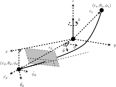
Figure 1: Schematic diagram for the deflection and lensing in the WDL in Kerr BH spacetime. The source and detectors are located at $(r_{s},\theta_{s},\phi_{s})$ and $(r_{d},\theta_{d},\phi_{d})$ respectively. The gray box represents a patch of the celestial plane of the detector. The apparent angles of the images on this plane are also indicated.

With the deflection in both $\theta$ and $\phi$ directions known, one then can attempt to solve the apparent angles of the GLed images using the GL equations. Such GL equations are usually built using some (approximate) geometrical relations linking the source and detector locations, the intermediate variables such as $r_{0}$ and $\theta_{\text{e}}$, the deflection angles $\Delta\phi,~{}\Delta\theta$, as well as the desired apparent angle(s), which has two components $(\alpha,~{}\beta)$ in our case. In Fig. 1, we adopt the common setup of the detector’s local inertial frame, whose basis axes consist of the detector-BH direction $\hat{r}_{s}$, and the directions $\hat{\theta}_{s}$ and $\hat{\phi}_{s}$ parallel respectively to the $\hat{\theta}$ and $\hat{\phi}$ basis of the spacetime coordinates.

In this work, our GL equations consist of two sets of equations. The first set is nothing but the very definition of the deflections in $\phi$ and $\theta$ directions

$$\Delta\phi(r_{0},\theta_{\text{e}})=\phi_{d}-\phi_{s}$$ (51a)

$$\Delta\theta(r_{0},\theta_{\text{e}})=\theta_{d}+\theta_{s}-\pi$$ (51b)

where $\Delta\phi$ and $\Delta\theta$ are expressed as in Eqs. (37) and (45). Using this set of equations, once the quantities $a,~{}M$ and $(r_{s},~{}\theta_{s},~{}\phi_{s}),~{}(r_{d},~{}\theta_{d},~{}\phi_{d}=2\pi)$ are given in prior, we will be able to solve the intermediate variables, i.e., the minimal radius $r_{0}$ and extreme $\theta$-coordinate $\theta_{\text{e}}$ that allow the signal to reach the detector. These two quantities can also be interchanged with the other pair of kinetic variables $(L,~{}E)$ of the signal. Note that without losing generality, we can always fix $\phi_{d}=2\pi$ and in the WDL, $\phi_{d}-\phi_{s}$ is usually very close to $\pi$. For later notation convenience, we will denote the small bending angle in the $\phi$-coordinates as $\delta\phi$, which is defined as

$$\delta\phi\equiv\phi_{d}-\phi_{s}-\pi=\pi-\phi_{s}$$ (52)

and the small bending angle in the $\theta$-coordinate as $\delta\theta$, which from Eq. (51b), is exactly $\Delta\theta$, i.e.,

$$\delta\theta\equiv\Delta\theta=\theta_{d}+\theta_{s}-\pi.$$ (53)

In practice, since Eqs. (37) and (45) have more complicated dependence on $r_{0}$ and $\theta_{\text{e}}$, we will use their expanded form of Eqs. (40) and (47) with terms of combined order higher than two truncated. Inspecting these two equations carefully, we can see that their dependence on $r_{0}$ can be converted to a polynomial form. From Eqs. (41f) and (48f), we observe that the 2nd order in the expansion of $(M/r_{0})$ is also the minimal order that the effect of the spacetime spin $\hat{a}$ will appear. Therefore any attempt to study the off-equatorial plane deflection and lensing should keep the deflection angles to at least this order, which is also what we will do in this work. For the dependence of this set of equations on $\theta_{\text{e}}$ however, we see that these two equations are both linear combinations of $\sin(nx_{s})$ and $\cos(nx_{s})~{}(n=0,~{}1,~{}2)$, which can also be converted to polynomials of $\tan(x/2)$. Unfortunately, to the order we desired, these polynomials do not allow simple analytical forms for their solutions. More precisely, in order to include the effect of $\hat{a}$, we found that the $\tan(x/2)$ should be a root of an order ten polynomial. Once $\tan(x/2)$ is obtained however, the $r_{0}$ is simply obtained by evaluating (not solving) a polynomial involving $\tan(x/2)$. Therefore we will use numerical method to solve $r_{0}$ and $\tan(x/2)$ in what follows.

In Figs. 2 - 5, we plot the solved $r_{0}$ and $\theta_{\text{e}}$ as functions of variables $\delta\phi,~{}\delta\theta,~{}\theta_{s},~{}\hat{a},~{}r_{s}$ by using the Sgr A* as the central lens. We used its data $M=4.1\times 10^{6}M_{\odot}$ and $r_{d}=8.34$ kpc [somerecentwork]. In principle, if we allow the spacetime spin to be negative and the status of the source and detector to be switched, then we can restrict the non-equivalent parameter space to $\delta\phi>0,~{}\delta\theta>0,~{}\theta_{s}\in[0,\pi/2]$. However, to show the GLed images more completely, in some of the plots in the following we will consider negative $\delta\theta,~{}\delta\phi$, $\delta\phi\in[-10,~{}10^{\prime\prime}]$ and $\delta\theta\in[-10,~{}10^{\prime\prime}]$ to be precise. The choice of other parameters is provided in the caption of each plot.

In general, we find that for each set of parameters and among the four different possible combinations of the signs $s_{r\theta}$ and $s_{l}$, there are only two combinations that allow physical solutions to $r_{0}$ and $\theta_{\text{e}}$. In general, one of the allowed trajectories will be prograde with respect to the positive spacetime spin axis (the $+z$ axis) and the other is retrograde. We will denote the minimal radii and extreme $\theta$-coordinate of the prograde trajectory as $(r_{0+},~{}\theta_{\text{e}+})$ and those of the retrograde trajectory as $(r_{0-},~{}\theta_{\text{e}-})$. Since $\theta_{s}\leq\pi/2$, when $\theta_{\text{e}}$ is a minimum (or maximum), the trajectory reaches the detector from above (or below) the equatorial plane, as illustrated in Fig. 1 by the two solid trajectories. Moreover, inspecting the lensing Eq. (51), we can see that all terms in these equations are even functions of $\theta_{\text{e}}-\pi/2$. This means that then for one solution $\theta_{\text{e}+}$ of these equations, there must exist another solution $\theta_{\text{e}-}=\pi-\theta_{\text{e}+}$. In other words, the two extremes $\theta_{\text{e}\pm}$ for prograde and retrograde motions must be supplementary to each other.

Before going into the details of the effect of each parameter, we would like to point out two fundamental properties of the trajectories that will help in the understanding of results in many following figures. The first is that when $\delta\phi$ is relatively large (greater than $10^{-4\prime\prime}$), the spacetime spin’s effect is only secondary compared to those of $\delta\phi$. This can be understood from Eq. **** that $\hat{a}$ appears one order higher than $\delta\phi$ or from the deflection angle that $\hat{a}$ appears one order higher than $M/r_{0}$. Under these parameter settings, then the effect of the spin can be ignored and the physics should be similar to the SSS case, in which the total deflection angle can be approximated as

$$\delta\eta\approx\sqrt{(\delta\theta)^{2}+\sin^{2}\theta_{s}(\delta\phi)^{2}}$$ (54)

Then from our experience with SSS spacetime, we knew that when $\delta\phi>0$, the minimal radius $r_{0+}$ will decrease while $r_{0-}$ will increase as $\delta\eta$ increase, as in Schwarzschild spacetime [5], regardless whether the increase of $\delta\eta$ is caused by the increase of $\delta\phi,~{}\theta_{s}$ or $\delta\theta$. Based on the first property, i.e., when the effect of $\hat{a}$ is secondary, the second feature of the trajectories is that they are basically within one plane containing the source, lens and detector. With these two fundamental properties in mind, one then can study and understand more easily how various quantities affect the extreme $\theta_{\text{e}\pm}$ by simply drawing this plane in the Cartesian coordinates.

Effect of various parameters

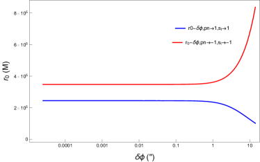
(a)

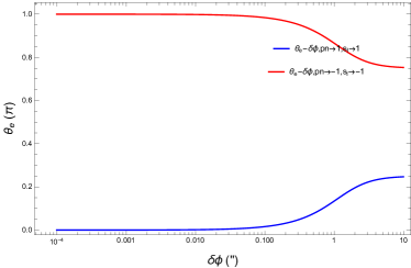
(b)

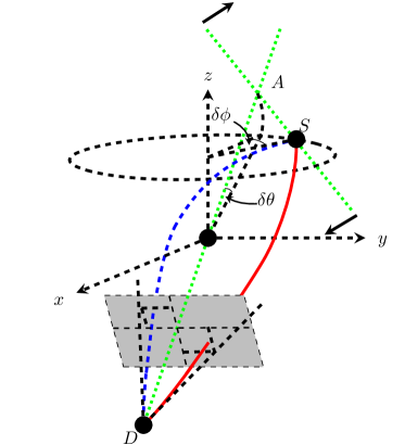
(c)

Figure 2: The dependence of $r_{0}$ and $\theta_{\text{e}}$ on $\delta\phi$. We fixed $\theta_{s}=\pi/4,~{}\delta\theta=1^{\prime\prime},~{}\hat{a}=1/2,~{}r_{s}=r_{d},~{}v=1$ in this plot.

Fig. 2 shows the dependence of $r_{0\pm}$ and $\theta_{\mathrm{e}\pm}$ on $\delta\phi$. This is one of the main relations studied in the GL in spherical symmetric or equatorial plane of axially symmetric spacetimes. As described above, for each set of fixed parameters, there are only two physical trajectories, which we denote as $(r_{0+},~{}\theta_{\text{e}+})$ for the prograde one and $(r_{0-},~{}\theta_{\text{e}-})$ for the retrograde one respectively. For the minimal radii, it is seen from Fig. 2 (a) that if the deflection $\delta\phi$ is larger than the deflection in the $\theta$-direction ($\delta\theta=1^{\prime\prime}$), then its effect to the bending of the trajectories would dominate those of the spacetime spin as well as $\delta\theta$, as can be seen from its contribution to the total deflection $\delta\eta$ in Eq. (54). As $\delta\phi$ decreases, $r_{0-}$ would rapidly decrease while $r_{0+}$ will increase, which is a feature qualitatively similar to the case in the equatorial plane [11]. However, as $\delta\phi$ approaches and becomes smaller than $\delta\theta=1^{\prime\prime}$, the effect of $\delta\theta$ to the bending will fix the two minimal radii at constant values, as shown by the flat regions in the left part of Fig. 2 (a). For the extreme $\theta_{\text{e}}$s of the two trajectories, it is seen from Fig. 2 (b) that as $\delta\phi$ decreases, the smaller (or larger) $\theta_{\text{e}+}$ (or $\theta_{\text{e}-}$) of the prograde (or retrograde) trajectory keeps decreasing (or increasing), indicating the trajectory is swung to near the $z$ axis above (or below) the equatorial plane. As $\delta\phi$ becomes much smaller than $\delta\theta$, the trajectories mainly bend in the $\theta$-direction, and the $\theta_{\text{e}+}$ and $\theta_{\text{e}-}$ approaches $\pi$ and $0$ indefinitely. We remind the readers that the $\theta$ coordinate along the trajectory does not necessarily deviate weakly from $\theta_{s,d}$ even in the WDL, which can be understood in the straight trajectory case in zero gravity. Fig. 2 (c) illustrate schematically the change of the trajectories as $\delta\phi$ changes.

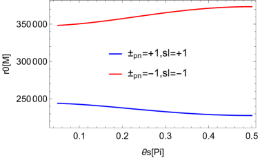
(a)

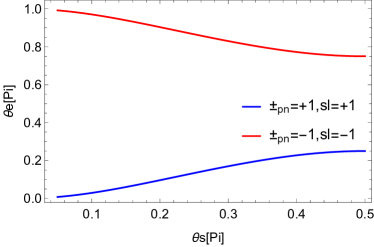
(b)

(c)

Figure 3: The dependence of $r_{0}$ and $\theta_{\text{e}}$ on $\theta_{s}$. We fixed $\delta\phi=1^{\prime\prime},~{}\delta\theta=1^{\prime\prime},~{}\hat{a}=1/2,~{}r_{s}=r_{d},~{}v=1$ in this plot.

Fig. 3 shows how $\theta_{s}$ affects $r_{0\pm}$ and $\theta_{\text{e}\pm}$. Note when adjusting $\theta_{s}$, we kept $\delta\theta=1^{\prime\prime}=\delta\phi$ a small constant so that $\theta_{d}$ is simultaneously adjusted. It is seen that first of all, compared to the effect of $\delta\phi$ on these quantities, that of $\theta_{s}$ is much weaker in general: a change of $\theta_{s}$ for about $\pi/2$ causes roughly the same amount of change for $\theta_{\text{e}\pm}$ and a smaller change of $r_{0\pm}$ than those by a change of $\delta\phi$ for $10^{\prime\prime}$. This is however expected both from Eq. (54) and the fact that the approximate alignment of the source-lens-detector is not changed dramatically in the process of $\theta_{s}$’s variation. The second feature is that the effects of $\theta_{s}$ to both $r_{0\pm}$ and $\theta_{\text{e}\pm}$ becomes stronger as $\theta_{s}$ decreases to zero, i.e., the $z$ axis pole directions, and weaker as it moves toward $\pi/2$, i.e., the equatorial plane. This is consistent with the first-order terms of Eq. (47), i.e., Eqs. (48b) and (48d), which are proportional to $\cos(x_{s})\to 0$ as $\theta_{s}$ approaches the equatorial plane, and can also be seen by differentiate Eq. (54) with respect to $\theta_{s}$.

For the effect of $\theta_{s}$ on $r_{0\pm}$, from Fig. 3 (a), we see that when the source and detectors are closer to the poles, the minimal radius $r_{0+}$ (and $r_{0-}$) for prograde (and retrograde) motion decreases (and increases) slightly. From our experience [5] with Schwarzschild spacetime with deflection $\delta\eta$ as given in Eq. (54), it is not hard to anticipate that the two minimal radii should basically take the shape shown in Fig. 3 (a) as $\theta_{s}$ varies. For extreme values of the $\theta$ coordinates, we see from Fig. 3 (b) that more polar source and detector locations yield more polar extreme $\theta_{\text{e}\pm}$. This can be understood from the second property we mentioned above that each trajectory lies basically in one plane containing the source, lens and detector. One can show by drawing this plane in the Cartesian coordinates that the closer the $\theta_{s}$ to the $+z$-axis, the closer the $\theta_{\text{e}\pm}$ to the poles. The change caused by the variation of $\theta_{s}$ is schematically shown in Fig.3 (c).

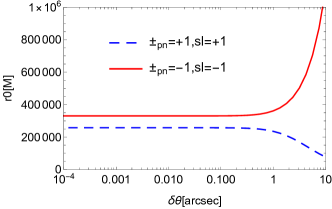
(a)

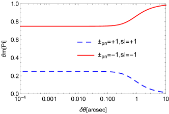
(b)

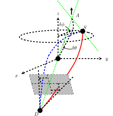
(c)

Figure 4: The dependence of $r_{0}$ and $\theta_{\text{e}}$ on $\delta\theta$. We fixed $\delta\phi=1^{\prime\prime},~{}\theta_{s}=\pi/4,~{}\hat{a}=1/2,~{}r_{s}=r_{d},~{}v=1$ in this plot.

The effect of $\delta\theta$ on $r_{0\pm}$ and $\theta_{\text{e}\pm}$, as shown in Fig. 4 , is related to the effects of $\theta_{s}$ itself in Fig. 3 and $\delta\phi$ in Fig. 2. Again, this is a consequence of the combination of these three parameters into the total deflection, as in Eq. (54). From Fig. 4 (a) we see that, as $\delta\theta$ increases to about $10^{\prime\prime}$, the $r_{0+}$ for prograde trajectory increases while $r_{0-}$ for retrograde trajectory decreases. The amount of their changes however is larger than those in Fig. 2 (a) because of the extra factor of $\sin^{2}\theta_{s}=1/2$ in Eq. (54). The apparent difference between the effect of $\delta\theta$ and $\delta\phi$ appears in their effects to the extreme $\theta$’s, $\theta_{\text{e}\pm}$. The increase of $\delta\theta$ with a fixed $\theta_{s}$ means the increase of $\theta_{d}$. Therefore for an increasing $\delta\theta$ but a fixed $\delta\phi$, one can draw the plane containing the source, lens and detector and find that the planes containing the two trajectories will be tilted more vertically towards the $z$-axis. When $\delta\phi>0$, this effectively increases $\theta_{\text{e}-}$ and decreases $\theta_{\text{e}+}$, as seen from Fig. 4 (b). The variation of the trajectories with the increase of $\delta\theta$ is schematically shown in Fig. 4 (c).

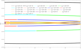
(a)

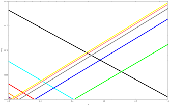
(b)

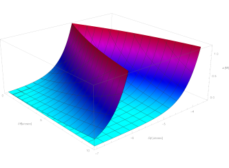
(c)

Figure 5: The dependence of $r_{0}$ (a) and $\theta_{\text{e}+}$ (b) on $\hat{a}$. Note that $\theta_{\text{e}-}=\pi-\theta_{\text{e}+}$. (c): the critical $a_{c}$. We fixed $\theta_{s}=\pi/4,~{}r_{s}=r_{d},~{}v=1$ in this plot.

Finally we plotted how the spacetime spin $\hat{a}$ affects the $r_{0\pm}$ and $\theta_{\text{e}\pm}$ in Fig. 5. As mentioned before, we found that when the total deflection $\delta\eta$ is larger than $\sim 10^{-5\prime\prime}$, the effect of $\hat{a}$ on these quantities are so weak that no noticeable changes are seen in these plots. Therefore we decreased in these figures $\delta\phi$ and $\delta\theta$ simultaneously from $10^{-5\prime\prime}$ to about $10^{-7}$’. As the deflections decrease, the influence of $\hat{a}$ starts to appear.

One of the most remarkable features that we observe in Fig. 5 (a-b), is that when $\delta\phi$ is small, there exists a transition between trajectories with different choices of $(s_{r\theta},s_{l})$ when $\hat{a}$ passes a critical value $\hat{a}_{c}$. When the $\delta\phi$ become sub-$\sim 10^{-5\prime\prime}$, the solutions of $(r_{0},\theta_{\text{e}})$ for $(s_{r\theta}=+1,s_{l}=+1)$ and $(s_{r\theta}=-1,s_{l}=-1)$ cease to exist when $\hat{a}$ is larger than $\hat{a}_{c}$. Instead, the solutions switch their sign choices to $(s_{r\theta}=+1,s_{l}=-1)$ and $(s_{r\theta}=-1,s_{l}=+1)$. This means for $\delta\phi>0,~{}\delta\theta>0$ and $\theta_{s}<\pi/2$, the signal reaching the detector from above (or below) switches from prograde to retrograde (or from retrograde to prograde). In other words, the two trajectories intersect with the $z$ axis at $a=a_{c}$ and therefore $\theta_{\text{e}\pm}=0,~{}\pi$ as confirmed in Fig. 5 (b) and illustrated in Fig. 5 (c).

This observation effectively provides us a criterion to solve for $a_{c}$: $\theta_{e}=0$. Substituting this into the lensing Eqs. (51), we are able to solve the critical $a_{c}$ to the leading order, as a of function of $\delta\theta,~{}\delta\phi$ and spacetime parameters. We see from this, as well as Fig. 5 (a,b), that the smaller the $\delta\phi$, the smaller this transition spin $|\hat{a}_{c}|$, indicating this switching of the signs is mainly a spacetime spin effect.

To clarify the property of $\hat{a}_{c}$, in Fig. 5 (c), we plot the exact dependence of $\hat{a}_{c}$ on $\delta\theta$ and $\delta\phi$ while holding other parameters such as $\theta_{s},~{}r_{s,d}$ etc. It is seen that if the spacetime is a BH one ($|\hat{a}|\leq 1$), then only for the small $\delta\phi$ within a finite region in the $\delta\theta\sim\delta\phi$ plane, there exists a critical $\hat{a}_{c}$ (the brown surface). For $\hat{a}$ below (or above) this surface, the trajectories as shown in Fig. 3 - 4 with signs $(s_{r\theta}=+1,s_{l}=+1)$ and $(s_{r\theta}=-1,s_{l}=-1)$ (or $(s_{r\theta}=+1,s_{l}=-1)$ and $(s_{r\theta}=-1,s_{l}=+1)$) are the physical solution.

There are a few other features worth remarking about this transition. Firstly, we see from this plot that the transition depends on $\delta\theta$ much weakly than on $\delta\phi$. This is understandable because $\hat{a}$ is along the direction around which $\phi$-coordinate evolves, but not the direction that $\theta$-coordinate. This is also consistent with our knowledge about the deflections in the equatorial plane, where the effect of spin $\hat{a}$ is most apparent only when $\delta\phi$ is very small [46]. Secondly, we also note that when $\delta\phi$ is small and fixed, the spin effect is stronger for larger $\delta\theta$ in that the corresponding $\hat{a}_{c}$ is smaller. Thirdly, this transition can also be viewed as caused by the variation of $\delta\theta$ or $\delta\phi$ when other parameters are fixed. That is, if we fix a constant $\hat{a}$, then for each $\delta\theta$ there exists a critical $\delta\phi$ below which, or similarly for each $\delta\phi$ there exists a critical $\delta\theta$ above which the sign choice for $(s_{r\theta},~{}s_{l})$ would be $(+,-)$ and $(-,+)$. Lastly, it is seen that when $\delta\phi$ is large or $\delta\theta$ is small, this $\hat{a}_{c}$ can exceed the extreme Kerr BH limit of 1, and therefore for these deflection angles the transition will not happen if we only consider the BH spacetime case. However, even for the Kerr spacetime with a naked singularity (the $\hat{a}>1$ part in this plot), we emphasize that this critical $\hat{a}_{c}$ still exists and our plot is still valid.

For $r_{0\pm}$, previously, it was known that in the equatorial plane, the increase of $\hat{a}$ will decrease the $r_{0+}$ and increase the $r_{0-}$ [46]. Seen from Fig. 5 (a), this trend is qualitatively unchanged in the off-equatorial plane case, and most apparent for very small deflections ($10^{-7\prime\prime}$ in Fig. 5 (a)). The influence of $\hat{a}$ on $\theta_{\text{e}\pm}$ although seems weak in size, is actually more interesting than its effect on $r_{0\pm}$. The $\theta_{\text{e}\pm}$ are very close to the $\hat{z}$ axis and at the transition $\hat{a}_{c}$, the trajectories intersect with the axis and therefore they are either $\pi$ or 0. When $\hat{a}$ decreases from being larger than $\hat{a}_{c}$ to smaller than that, the trajectory that attained a minimal $\theta$-value at almost zero becomes a trajectory with a maximal $\theta$-value around $\pi$. An opposite transition happens for the other trajectory. Finally, let us also point out the simple fact that when $\hat{a}<0$, the prograde and retrograde trajectories actually rotate clockwise and anti-clockwise respectively against the $+\hat{z}$ direction.

IV.2 The apparent angles and magnifications

Apparent angles

Once $(r_{0},~{}\theta_{\text{e}})$ or $(L,E)$ are solved for a given set of small $\Delta\theta-\pi$ and $\Delta\phi$, previously based on some approximate geometrical relations, Refs. [42, 43] have developed an approximate formula for the apparent angles of the images. However here, we will use the following exact definition of the apparent angles derived using the projection of the signal trajectory onto the lens-observer axis

$$\alpha=\sin^{-1}\frac{L(\Delta_{d}-a^{2}s_{d}^{2})+2aM{E}r_{d}s_{d}^{2}}{s_{d}\sqrt{\Delta_{d}\Sigma_{d}({E}^{2}\Sigma_{d}-m^{2}(\Delta_{d}-a^{2}s_{d}^{2}))}}.$$ (55)

$$\beta=\sin^{-1}\frac{s_{r\theta}\sqrt{\Theta(c_{d})(\Delta_{d}-a^{2}s_{d}^{2})}}{s_{d}\sqrt{\Sigma_{d}\left[{E}^{2}\Sigma_{d}-m^{2}(\Delta_{d}-a^{2}s_{d}^{2})\right]}},$$ (56)

$$\alpha=\frac{s_{l}{r_{0}}\sin(x_{d})}{r_{d}}+\frac{s_{l}M\sin(x_{d})}{r_{d}v^{2}}{}$$

$$-\frac{\sin(x_{d})}{2{r_{0}}{r_{d}}}\left(-s_{l}a^{2}+\frac{{s_{e}}4aM}{v}+\frac{s_{l}M^{2}}{v^{4}}\left(1-4v^{2}\right)\right){}$$

$$-\frac{Ms_{l}{r_{0}}\sin(x_{d})}{r_{d}^{2}v^{2}}+\frac{s_{l}{r_{0}}^{3}\sin^{3}(x_{d})}{6{r_{d}}^{3}},$$ (57)

$$\beta=\frac{s_{r\theta}M\cos(x_{d})}{r_{d}v^{2}}+\frac{s_{r\theta}{r_{0}}\cos(x_{d})}{r_{d}}-\frac{s_{r\theta}M{r_{0}}\cos(x_{d})}{r_{d}^{2}v^{2}}{}$$

$$+\frac{s_{r\theta}\cos(x_{d})}{2r_{0}r_{d}}\left(-a^{2}s_{e}^{2}\csc^{2}(x_{d})+a^{2}-\frac{4s_{l}aMs_{e}}{v}\right.{}$$

$$\left.+\frac{M^{2}}{v^{4}}\left(4v^{2}-1\right)\right)+\frac{s_{r\theta}{r_{0}}^{3}\cos^{3}(x_{d})}{6{r_{d}}^{3}},$$ (58)

For the derivation of these formulas, see Appendix C. Note that the $r_{0\pm}$ and $\theta_{\text{e}\pm}$ enter these apparent angles through the angular momentum $L$ and the Carter constant $K$, which appears in $\Theta(c_{d})$. These formulas have the advantage that they are applicable regardless of whether the signal was bent weakly or strongly, although we only focus on the former case in this work. We have also verified in the WDL and equatorial plane limit, $\beta\to 0$ and $\alpha$ yield the corresponding results in Ref. [11] (after switching from impact parameter to $r_{0}$). Moreover, if we are interested in a single apparent angle $\gamma$ between the signal and the direction of the Kerr BH, then this is given by Eq. (103)

$$\gamma= \cos^{-1}\left\{\frac{[(aL-(a^{2}+r_{d}^{2}){E})^{2}-(K+m^{2}r_{d}^{2})\Delta_{d}]}{\Delta_{d}\Sigma_{d}\left[{E}^{2}\Sigma_{d}-m^{2}(\Delta_{d}-a^{2}s_{d}^{2})\right]}\right.{}$$

$$~{}~{}~{}~{}~{}~{}~{}~{}\times(\Delta_{d}-a^{2}s_{d}^{2})\bigg{\}}^{1/2}.$$ (59)

Since $r_{s,d}\gg r_{0}\gg M\geq\hat{a}$, we can expand the

To the leading order of $r_{0}/M$, it is not difficult to show that $\gamma\approx\sqrt{\alpha^{2}+\beta^{2}}$.

To reveal the dependence of the image positions on parameters $\delta\phi,~{}\theta_{s},~{}\delta\theta$ and $\hat{a}$, in Figs. 6, we plot the angular locations $(\alpha_{\pm},~{}\beta_{\pm})$ of the prograde and retrograde images formed by trajectories with $(r_{0\pm},~{}\theta_{\text{e}\pm})$ in the celestial plane shown in Fig. 1. Note that if the lens was absent, it is easy to find that the source would appear to be at the point

$$(\alpha,~{}\beta)=\left(\frac{r_{s}\sin\theta_{s}\delta\phi}{r_{s}+r_{d}},~{}-\frac{r_{s}\delta\theta}{r_{s}+r_{d}}\right)$$ (60)

on the celestial plane of the observer.

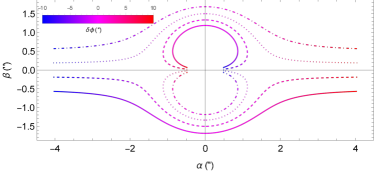
(a)

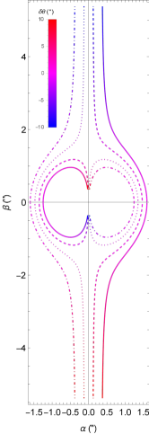
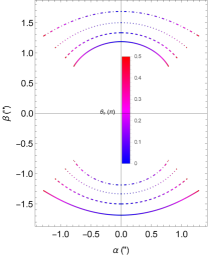
(b)                          (c)

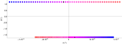
(d1)

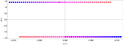
(d2)

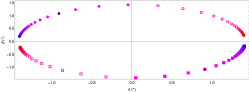
(d3)

Figure 6: The dependence of the apparent angles $(\alpha,~{}\beta)$ on $\delta\phi$ from $-10^{\prime\prime}$ to $10^{\prime\prime}$ (a), on $\delta\theta$ from $-10^{\prime\prime}$ to $10^{\prime\prime}$ (b), and on $\theta_{s}$ from $0.01\pi$ to $\pi/2$ (c), and $\hat{a}$ from -1 to 1 in (d) for $\delta\phi=10^{-6\prime\prime}$ and three $\delta\theta=1^{\prime\prime}$ (d1) $\delta\theta=10^{-3\prime\prime}$ (d2) and $\delta\theta=10^{-6\prime\prime}$ (d3). Different line types in (a), (b), (c) are for different values of $\delta\theta,~{}\delta\phi$ and $\delta\theta=\delta\phi$. The solid, dashed, dot-dashed and dotted lines represent $1^{\prime\prime},~{}0.33^{\prime\prime},~{}-0.33^{\prime\prime},~{}-1^{\prime\prime}$ respectively. The default values of parameters in each subplot, except those varied, are $\delta\theta=1^{\prime\prime},~{}\delta\phi=1^{\prime\prime},~{}\hat{a}=1/2,~{}r_{s}=r_{d},~{}v=1$.

In Fig. 6 (a), we vary continuously the $\phi$-coordinate and consequently $\delta\phi$ of the source while keeping $\theta_{s}$ and $\hat{a}$ fixed and show the location of the images for several discrete $\delta\theta$. The value of $\delta\phi$ is color-coded so that basically the left side of the curves corresponding to $\delta\theta=-10^{\prime\prime}$ and the right side to $\delta\theta=10^{\prime\prime}$. It is seen that for each fixed set of parameters in the chosen parameter range, there always come two conjugate images distributed in opposite quadrants, on the same straight line passing the origin. For $\hat{a}=1/2>0$ and $\delta\theta>0$, the image pairs in the first and third (or the fourth and second) quadrants are when $\delta\phi<0$ (or $\delta\phi>0$) and correspond to retrograde and prograde signals respectively. For $\hat{a}=1/2>0$ and $\delta\theta<0$, the opposite happens. In each pair of the images, the one on the outer curves has a larger minimal radius and the one on the inner circular curves has a smaller $r_{0}$, corresponding to retrograde and prograde images respectively. Since for the chosen parameter ranges of $\delta\theta$ and $\delta\phi$, the effect of $\hat{a}$ is not apparent (see Fig. 5), the lens images look almost symmetric for $\delta\theta$ or $\delta\phi$ with opposite signs.

Among each pair of the images, it is seen that for each fixed $\delta\theta$, with the decreasing of $\delta\phi$, the $\alpha$-coordinate of the far-side image increase monotonically. Again, the reason is simply that the variation of the $\phi$-coordinate of the source is indeed parallel to the $\alpha$-axis in the celestial plane. The qualitative features of the angular locations of the inner images are actually more interesting. When $\delta\phi$ increases to large values, it is seen that although the $\beta$ coordinates of the outer images do not approach zero, that of the inner images do. While when $|\delta\phi|$ decreases from large values, the $\alpha$ coordinates of the inner images do not decrease monotonically, but increase to a maximal value first and then decrease, indicating that the effect of $\delta\phi$ starts to dominate the image locations. This last feature is actually in accord with Fig. 2 (c).

Fig. 6 (b) shows the dependence of the image locations on $\delta\theta$ for a few fixed $\delta\phi$. Qualitatively, this figure looks similar to a rotation of Fig. 6 (a), indicating that the role of $\delta\phi$ in Fig. 6 (a) is now played by $\delta\theta$ and vice versa. An apparent difference is that the range of the $\beta$ angle in Fig. 6 (b) is about $1.4\approx\sqrt{2}=1/\sin\theta_{s}$ times that of the $\alpha$ angle in Fig. 6 (a). This is a reflection of the $\sin\theta_{s}$ factor in the contribution of $\delta\theta$ and $\delta\phi$ to the total deflection in Eq. (54).

In Fig. 6 (c) we illustrate the effect of $\theta_{s}$ on the image location when fixing $\delta\phi=\delta\theta=1^{\prime\prime}$. It is seen that when $\theta_{s}$ approaches the spacetime rotation axis, both the corresponding images are shifted to the location very close to the $\alpha$ axis too, which is consistent with the fact that both $\theta_{\text{e}\pm}$ approach the $\hat{z}$ axis in Fig. 3 (b). When $\theta_{s}$ turns to $\pi/2$ however, the images do not approach zero $\beta$ but only some finite $\beta$ that is smaller than $\delta\theta$. This is also in accord with the observation from Fig. 3 (b) that the $\theta_{\text{e}\pm}$ approach only some middle values not close to either 0 or $\pi/2$. The more fundamental reason for these phenomena is simply that $\delta\theta$ is still non-zero in this case, i.e., the detector is still below the equatorial plane. In general, the apparent angle $\gamma\approx\sqrt{\alpha^{2}+\beta^{2}}$ in this figure is not changed much as $\theta_{s}$ varies, because in this case the total effective deflection given by Eq. (54) is not changed by a large factor.

For the ranges of parameters considered in Fig. 6 (a)-(c), it is actually easy to verify that the critical situation for which $\hat{a}$’s effect becomes apparent is never reached. Therefore for these parameter ranges, in principle, we expect that the apparent angles can be well approximated by the results in Schwarzschild spacetime. There, when the source is located on the equatorial plane, the apparent angles to the leading order are [45]

$$\alpha_{S,\pm}= \frac{r_{s}\sqrt{\delta\theta^{2}+\sin^{2}\theta_{s}\delta\phi^{2}}}{2(r_{s}+r_{d})}\left(\text{sgn}(\delta\phi)\mp\zeta\right),$$ (61)

$$\text{where}~{}\zeta= \sqrt{1+\frac{8M(r_{d}+r_{s})\left(1+\frac{1}{v^{2}}\right)}{r_{d}r_{s}(\delta\theta^{2}+\sin^{2}\theta_{s}\delta\phi^{2})}}.$$ (62)

Here we have replaced the $\delta\phi$ in the Schwarzschild spacetime with the total deflection $\delta\eta$ in the Kerr spacetime, i.e., Eq. (54). However, since the source now is not located on the equatorial plane, these images should be rotated on the celestial plane such that the trajectories are in roughly the same plane as the source, lens and detector. The location of the source with the absence of the lens in Eq. (60) provides for the images a rotation angle $\xi$ from the projection of the $+\hat{\alpha}$ axis on the celestial plane such that

$$\cos\xi=\sin\theta_{s}\delta\phi/\delta\eta,~{}\sin\xi=-\delta\theta/\delta\eta.$$ (63)

Applying the above rotation to the apparent angles in Eq. (62), we finally find the apparent angles $(\alpha_{\pm},~{}\beta_{\pm})$ for sources in Kerr spacetimes as

$$\alpha_{\pm}= \frac{\sin\theta_{s}\delta\phi\,r_{s}}{2(r_{s}+r_{d})}\left(1\mp\text{sgn}(\delta\phi)\zeta\right),$$ (64)

$$\beta_{\pm}= \frac{-\delta\theta\,r_{s}}{2(r_{s}+r_{d})}\left(1\mp\text{sgn}(\delta\phi)\zeta\right),$$ (65)

where $\zeta$ is in Eq. (62). We redrew the image locations $(\alpha_{\pm},~{}\beta_{\pm})$ using the above equations for parameters given in the caption of Fig. 6 (a) - (c) and found excellent agreement with these figures. Besides, these formulas also can be used to explain the relevant results in Ref. [37].

Fig. 6 (d1)-(d3) show the effect of $\hat{a}$ on the apparent angles of the images. We intentionally choose small but positive $\delta\phi$ so that $\hat{a}$ can pass the critical $\hat{a}_{c}$ discussed in Fig. 5 as it varies from -1 to 1. What is most interesting in these plots, and in contrast to the cases in (a)-(c) where the effect of $\hat{a}$ is not evident, is the feature that the apparent angle of a retrograde (or prograde) signal with a negative orbital angular momentum $s_{l}=+1$ (or negative $s_{l}=-1$) can extend to the $\alpha<0$ (or $\alpha>0$) region. This means that as $\hat{a}$ increase before reaching $\hat{a}_{c}$, the prograde (or retrograde) trajectory can appear to be from the positive (or negative) $\alpha$ side.

Magnifications

The magnification of the images is defined as the ratio between the observed image angular size to the source angular size if the lens was absent

$$\mu= \frac{\mathrm{d}\Omega_{i}}{\mathrm{d}\Omega_{i}^{\prime}}=\frac{(r_{d}+r_{s})^{2}}{r_{s}^{2}\sin\theta_{d}}J{}$$

$$= \frac{(r_{d}+r_{s})^{2}}{r_{s}^{2}\sin\theta_{d}}\left|\displaystyle\begin{array}[]{cc}\frac{\partial\alpha}{\partial(\delta\theta)}&\frac{\partial\alpha}{\partial(\delta\phi)}\\ \frac{\partial\beta}{\partial(\delta\theta)}&\frac{\partial\beta}{\partial(\delta\phi)}\end{array}\right|$$ (68)

where $J$ is the Jacobian of the transformation shown above. This agrees with Ref. [38] which considered the (quasi-)equatorial plane case.

Using the Eqs. (55) and (56), the $(\alpha,~{}\beta)$ are conneted to $(L,\Theta)$, which according to Eqs. (11) and then (19) and (20), are functions $(r_{0},~{}\theta_{\text{e}})$. These quantities can be finally connected to $\delta\theta$ and $\delta\phi$ through solutions of $\theta_{\text{e}}$ and $r_{0}$. Therefore, using the chain rule for the partial derivatives, each element in the Jacobian can be computed as

$$\frac{\partial\alpha}{\partial(\delta\theta)}=\frac{\mathrm{d}\alpha}{\mathrm{d}L}\left(\frac{\partial L}{\partial r_{0}}\frac{\partial r_{0}}{\partial(\delta\theta)}+\frac{\partial L}{\partial\theta_{\text{e}}}\frac{\partial\theta_{\text{e}}}{\partial(\delta\theta)}\right),$$ (69a)

$$\frac{\partial\alpha}{\partial(\delta\phi)}=\frac{\mathrm{d}\alpha}{\mathrm{d}L}\left(\frac{\partial L}{\partial r_{0}}\frac{\partial r_{0}}{\partial(\delta\phi)}+\frac{\partial L}{\partial\theta_{\text{e}}}\frac{\partial\theta_{\text{e}}}{\partial(\delta\phi)}\right),$$ (69b)

$$\frac{\partial\beta}{\partial(\delta\theta)}=\frac{\mathrm{d}\beta}{\mathrm{d}\Theta}\left[\left(\frac{\partial\Theta}{\partial L}+\frac{\partial\Theta}{\partial K}\frac{\partial K}{\partial L}\right)\left(\frac{\partial L}{\partial r_{0}}\frac{\partial r_{0}}{\partial(\delta\theta)}+\frac{\partial L}{\partial\theta_{\text{e}}}\frac{\partial\theta_{\text{e}}}{\partial(\delta\theta)}\right)\right.{}$$

$$\left.~{}~{}~{}~{}~{}~{}~{}~{}~{}+\frac{\partial\Theta}{\partial K}\frac{\partial K}{\partial\theta_{\text{e}}}\frac{\partial\theta_{\text{e}}}{\partial(\delta\theta)}\right],$$ (69c)

$$\frac{\partial\beta}{\partial(\delta\phi)}=\frac{\mathrm{d}\beta}{\mathrm{d}\Theta}\left[\left(\frac{\partial\Theta}{\partial L}+\frac{\partial\Theta}{\partial K}\frac{\partial K}{\partial L}\right)\left(\frac{\partial L}{\partial r_{0}}\frac{\partial r_{0}}{\partial(\delta\phi)}+\frac{\partial L}{\partial\theta_{\text{e}}}\frac{\partial\theta_{\text{e}}}{\partial(\delta\phi)}\right)\right.{}$$

$$\left.~{}~{}~{}~{}~{}~{}~{}~{}~{}+\frac{\partial\Theta}{\partial K}\frac{\partial K}{\partial\theta_{\text{e}}}\frac{\partial\theta_{\text{e}}}{\partial(\delta\phi)}\right].$$ (69d)

Substituting $r_{0\pm}$ and $\theta_{\text{e}\pm}$ for each image into the above equation, one would immediately obtain their corresponding magnifications. We will use $\mu_{+}$ and $\mu_{-}$ respectively to represent the magnification for the prograde and retrograde images.

When $\delta\theta$ is large so that the effect of $\hat{a}$ is weak, then this magnification can be simplified to that of a Schwarzschild spacetime

$$\mu_{\pm}= \frac{u^{2}+2}{2u\sqrt{u^{2}+4}}\mp\text{sgn}(\delta\phi)\frac{1}{2},$$ (70)

$$\text{where}~{}u= \sqrt{\frac{r_{d}(r_{s}+r_{d})(\delta\theta^{2}+\sin^{2}\theta_{s}\delta\phi^{2})}{2Mr_{s}\left(1+\frac{1}{v^{2}}\right)}}.$$ (71)

and the total deflection $\delta\eta$ in Eq. (54) has replaced the corresponding deflection $\delta\phi$ in the Schwarzschild spacetime. From this, the effect of parameters $\delta\phi,~{}\delta\theta,~{}\theta_{s}$ are very apparent.

In Fig. 7 we show the dependence of the magnification on the parameters $\delta\phi,~{}\delta\theta,~{}\theta_{s}$ and $\hat{a}$. Other parameters in each figure are the same as in Fig. 6. It is seen from Fig. 7 that the magnifications $\mu_{\pm}$ for both images decrease as any of the deflection angles $\delta\phi,~{}\delta\theta$ increase. Moreover, the magnification $\mu_{+}$ of the prograde image decreases to zero while $\mu_{-}$ of the retrograde image decreases to $1$, which are the asymptotic values of Eq. (70). When both deflections $\delta\phi$ and $\delta\theta$ are small, both magnifications $\mu_{\pm}$ become very large. The above features are qualitatively similar to the magnifications of lensed images in SSS spacetimes but with the total deflection angle $\delta\eta$ in (54) playing the rule of deflection in SSS spacetime [45].

For a fixed $\hat{a}$, these magnifications start to deviate from the SSS case if the $\delta\theta$ and $\delta\phi$ are such that $\hat{a}$ becomes close to its critical value $\hat{a}_{c}$. This is however different from the SSS case because there, when the total deflection is zero, the magnification of the Einstein ring is actually divergent [45]. Therefore, we can attribute this difference to the presence of the spacetime spin. This is actually verified in Fig. 7 (b) where we plot the same magnifications for a very small $\hat{a}$, as one can see that the central value becomes much larger.

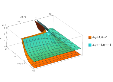
(a)

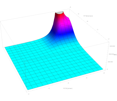
(b)

Figure 7: The dependence of the magnification on $\delta\phi$ and $\delta\theta$ (a). We fixed $\theta_{s}=\pi/4,~{}\hat{a}=1/2,~{}r_{s}=r_{d},~{}v=1$ in this plot.

V Applications

In this section, we discuss a few issues that our results above can be used to study.

V.1 Image track of moving sources

We will first study the images of a source not moving inequatorial plane behind the lens. Such sources can include stars whose or other transits whose orbit (almost) intersects with the observer-lens axis and whose angular velocity is appreciable so that observation becomes possible, e.g., some S stars around Sgr A*.

In Fig. 8, we assume that the source is located at some representative radius of the S star orbits, and plot the location of the GLed image of this source as it moves across. Since we only work in a WDL, for the section of the trajectory that we can treat, basically the trajectory looks almost a straight line if there was no lens. We assume that this straight line satisfies the parametric relation $\delta\phi=\delta_{0}+\delta\theta$ where $\delta_{0}$ takes a few values $10^{-5\prime\prime},10^{-3\prime\prime},10^{-1\prime\prime}$ and $\delta\theta$ runs from $-10^{\prime\prime}$ to $10^{\prime\prime}$ in Fig. 8 in order to compute the corresponding image locations.

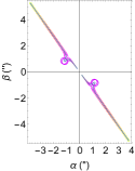
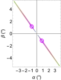
(a)                 (b)                 (c)

Figure 8: The dependence of the apparent image and magnification on moving sources, where$\delta\phi=\delta_{0}+\delta\theta$ and $\delta\theta$ from $0$ to $10^{\prime\prime}$(a1,b1,c1) and $\delta\theta$ from $0$ to $-10^{\prime\prime}$(a2,b2,c2). We fixed $\hat{a}=1/2,\theta_{s}=\frac{\pi}{4},~{}r_{s}=r_{d},~{}v=1$ and $\delta_{0}=10^{-1\prime\prime}$(a1,a2), $\delta_{0}=10^{-3\prime\prime}$(b1,b2), $\delta_{0}=10^{-5\prime\prime}$(c1,c2)in this plot.

It is seen that when $\delta_{0}$ is relatively large, the …

V.2 Shape of lensed images

Among possible sources GLed by a Kerr BH, stars or other spherical shape objects are very natural candidates. If the source and/or the lens are small and too far from us so that the shape of the images are not resolvable, then only the central values of the apparent angles $(\alpha,~{}\beta)$ might be obtained. However when the source is large or close and the detector has enough resolution, then the shape of the source should also be recognizable. In an SSS spacetime, then one would expect that the images of a spherical source would generally take elongated shapes.

In the Kerr spacetime, if the $\delta\theta$ and $\delta\phi$ are large so that the effect of $\hat{a}$ is much weaker on the trajectory deflection, then naturally one would expect that the shape of the images will be similar to those in the Schwarzschild spacetime with $\delta\eta$ in Eq. (54) playing the rule of the source’s deflection. In this case, we can work out the shape of the images based on the apparent angle formula (62) in the Schwarzschild spacetime. Supposing that the source object’s radius is $R$ and $R/r_{s}\ll\delta\eta$ (see Fig. 9), and denoting the angle of a boundary point to be $\sigma$, then to the leading order of $R/r_{s}$, the deflection angle of the boundary point with respect to the Schwarzschild lens becomes

$$\delta\eta^{\prime}=\delta\eta+\frac{R}{r_{s}}\sin\sigma+\mathcal{O}\left(\frac{R}{r_{s}}\right)^{2}.$$ (72)

Substituting this into Eq. (62) and to the first order of $R/r_{s}$, the two images now have apparent angles

$$\alpha_{S,\pm}^{\prime}= \alpha_{S,\pm}+\frac{R}{2(r_{d}+r_{s})}\left(\text{sgn}(\delta\phi)\mp\frac{1}{\zeta}\right)\sin\sigma$$ (73)

$$\equiv \alpha_{S,\pm}+\delta\alpha_{S,\pm},$$ (74)

where the last term is defined as the small variation $\delta\alpha_{\pm}$ of the apparent angle in the radial direction of the images. While the extension of the images in the direction perpendicular to $\alpha$ is

$$\delta\beta_{\pm}=\frac{R\cos\sigma}{r_{s}}\frac{\alpha_{S,\pm}}{\delta\eta}.$$ (75)

Eqs. (74) and (75) clearly demonstrate that the images have elliptic shapes with $\delta\alpha_{\pm}$ being the semi-minor axis and $\delta\beta_{\pm}$ the semi-major axis and the semi-minor axis is aligned with the image-lens axis. The eccentricity of these ellipses are

$$e_{\pm}=\frac{|\delta\beta_{\pm}|-|\delta\alpha_{S,\pm}|}{|\delta\beta_{\pm}|+|\delta\alpha_{S,\pm}|}=\frac{\zeta-1}{\zeta+1}.$$ (76)

The corresponding magnifications are the ratio between the angular size of the images and the original source

$$\mu_{\pm}= \left|\frac{\pi\delta\alpha_{S,\pm}/\sin\sigma\cdot\delta\beta_{\pm}/\cos\sigma}{\pi R^{2}/(r_{s}+r_{d})^{2}}\right|{}$$

$$=\pm\frac{1}{4}\left(1\pm\text{sgn}(\delta\phi)\frac{1}{\zeta}\right)\left(1\pm\text{sgn}(\delta\phi)\zeta\right).$$ (77)

One can check that this agrees with the magnification (70) for images of the source at $\delta\eta$.

In Fig. 9 we show the image locations of a star with twice size of our Sun and located at $r_{s}=100^{\prime\prime}r_{d}$ and $\delta\theta=\delta\phi=1^{\prime\prime}$. One can see that they do take the elliptic shape and we have checked that their eccencity and magnifications match exactly the values specified by Eqs. (76) and (77).

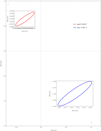
Figure 9: The apparent image $(\alpha,~{}\beta)$ of a star with twice the Sun’s size. We fixed $s_{r\theta}=+1,~{}s_{l}=+1,~{}\theta_{s}=\pi/4,~{}\delta\phi=\delta\theta=1^{\prime\prime},~{}\hat{a}=1/2,~{}r_{s}=r_{d},~{}v=1$. The red, blue and the black dashed line are the two GLed images and the source shapde without the presence of the lens (the inset is the zoomed-in images).

V.3 Constraining the BH and source

Kerr BH spacetime is thought as the most important BH in astronomy, while the SMBH Sgr A* is currently the best confirmed BH candidate. However, even such there are still much information regarding the Sgr A* that are not well constrained. For Sgr A*, whose jet is not apparent, then both its spin size and orientation with respect to the line-of-sight are not constrained well.

However, if the images of a source that is well aligned with the detector-lens axis (small $\delta\phi$) are observed, then we might attempt to constrain the spin of the BH, as well as other parameters such as the source distance $r_{s}$, using the observables described in previous sections. Among the input parameters $\{M,~{}a,~{}\theta_{s},~{}r_{s},~{}r_{d},~{}\delta\theta,~{}\delta\phi,~{}v\}$, the parameters $M,~{}\hat{a}$ and $\theta_{s}$, which together with the parameters $\psi$ describes the orientation of the BH spin, are associated with the BH itself. The parameters $r_{s},~{}\delta\theta$ and $\delta\phi$ are associated with the source and $r_{d},~{}v$ are associated with the detector and signal respectively. Usually the parameters $M,~{}r_{d}$ can be obtained from other means and we can set $v=1$ for light signals. $\delta\theta,~{}\delta\phi$ normally can not be measured while $r_{s}$ sometimes can be deduced from the spectrum redshift if the source is a far-away galaxy but would be more difficult to measure for a typical star in the Galaxy. The spacetime parameters $\hat{a}$ and $\theta_{s}$ are then the main quantity we want to constrain using observables considered in this paper.

We assume that for a GL situation by a Kerr BH, we can observe the two images’ relative positions $\gamma_{\pm}$ against the central BH and the opening angle $\lambda$ between them, and their relative flux ratio $\bar{\mu}$, and potentially the time delay $\Delta\tau$. Assuming the projection of $\hat{a}$ on the celestial plane is characterized by an angle $\psi$, then the above means the following relations

$$\alpha_{+}= \gamma_{+}\cos(\lambda-\psi),$$ (78a)

$$\beta_{+}= \gamma_{+}\sin(\lambda-\psi),$$ (78b)

$$\alpha_{-}= \gamma_{-}\cos\psi,$$ (78c)

$$\beta_{-}= -\gamma_{-}\sin\psi,$$ (78d)

$$\mu_{+}+\mu_{-}= 2\bar{\mu},$$ (78e)

These six constraints allow us to solve unknowns $\delta\theta,~{}\delta\phi,~{}\psi$ and the interested quantities $\hat{a},~{}\theta_{s},~{}r_{s}$. If the time delay between the images is not measured, then we will have to fix one quantity a priori, e.g. $r_{s}$, using other means.

$\gamma_{+}~{}(^{\prime\prime})$	$\gamma_{-}~{}(^{\prime\prime})$	$\pi-\lambda~{}(^{\prime\prime})$	$\bar{\mu}$	$\hat{a}~{}(M)$	$\theta_{s}$	$\psi$	$r_{s}~{}(M)$
$0.013937$	$0.013935$	$6.998*10^{-9}$	$4061.8$	$1/2$	$\pi/4$	$2.808*10^{-5}$	$2.06*10^{6}$

Table 1: Deduction of BH spin and orientation and source location from observables. Columns 1 - 5 are observables, and 6 - 9 are solved quantities.

In Table 1 we present in column 7 - 10 the results of $\hat{a},~{}\theta_{s},~{}\psi,~{}r_{s}$ using the assumed observations in column 1 - 6. The less interesting $\delta\theta,~{}\delta\phi$ are not shown.

VI Discussions

This work considered the deflection and GL of both null and timelike signals in off-equatorial plane in Kerr spacetime in the WDL. The deflection angles are computed using the perturbative method and the result are power series of $M/r_{0}$ and $r_{0}/r_{s,d}$ with the coefficients being functions of the spacetime parameter and the trogonometric function of the extreme values $\theta_{\text{e}}$ along the trajectories. Also importantly, the finite distance effect of the source and detectors are taken into account in these deflections. This allows us to establish a set of exact GL equations, from which we can solve the desired $(r_{0},\theta_{\text{e}})$ allowing the signal from a source with deflections $\delta\theta$ and $\delta\phi$ to reach the detector.

Using the exact formula for the apparent angles derived for the off-equatorial plane signals, we study the effect of various parameters, including the source deflection $\delta\theta,~{}\delta\phi$, the spacetime spin $\hat{a}$ and its orientation $\theta_{s}$, on the angular locations of the images on the celestial plane and their magnifications. It is generally found that, there exist usually two trajectories that will reach the detector. For a given $\delta\theta$ and $\delta\phi$, there always exists two critical $\hat{a}_{c}$ at which the two signal intersect the spin positive and negative directions directions respectively. Generally, when $\delta\theta$ or $\delta\phi$ are large, the effect of $\hat{a}$ (for the Kerr BH $\hat{a}\leq 1$) becomes subdominate and therefore the GL is roughly the same as that in the Schwarzschild spacetime (but off-equatorial plane). However in other case, $\hat{a}$ will affect the quadrant in which the images appear, and the magnification of these images.

We used these results to study the image of a transiting source behind the lens, the image shape and size of a spherical source, and using the observables to deduce properties of the BH and its orientation.

There are a few points that we can discuss here. The first is that in principle, it is not difficult to find the total travel time for a signal and then the time delay between the images. We plan to carry out this computation soon. The second is that, it seems from the mathematical point of view, the perturbation method should be generalizable to the deflection and GL in off-equatorial plane of other axisymmetric spacetime. We are exploring the detailed condition for this idea to work too.

Appendix A Integrability of the series

In this appendix, we show that the integrals of the forms (25) and (26) are always integrable and the results are elementary functions of the limits.

For the integral (25), multiplying the numerator and denominator of the integrand by $(1-p)^{i-1}$, each power in the integrand is transformed to the left-hand side of the following equation

$$\int_{1}^{p_{s,d}}\frac{p^{k}\mathrm{d}p}{\left(1-p^{2}\right)^{i-1/2}}=\left.-\frac{p^{k-1}}{(2i+k-4)\left(1-p^{2}\right)^{i-3/2}}\right|_{1}^{p_{s,d}}$$

$$+ \frac{k-1}{2i+k-4}\int_{1}^{p_{s,d}}\frac{p^{k-2}\mathrm{d}p}{\left(1-p^{2}\right)^{i-1/2}},~{}~{}(k+1,i=1,2,\cdots)$$ (79)

where the integration is done by parts. Note that superficially the first term on the right-hand side might diverge when $p$ approaches $1$. However, all these divergences will cancel when substituting these results into Eq. (25) because this is an artifact introduced when multiplying its integrand denominator by $(1-p)^{i-1}$. The recursion relation (79) allows us to lower the order of the numerator by 2. Finally, for the lowest two orders $k=0,~{}1$ cases, we have

$$\int_{1}^{p_{s,d}}\frac{\mathrm{d}p}{\left(1-p^{2}\right)^{i-1/2}}= \sum^{i-2}_{k=0}\frac{C^{k}_{i-2}}{2k+1}\left.\frac{p^{2k+1}}{\left(1-p^{2}\right)^{i+1/2}}\right|_{1}^{p_{s,d}},$$ (80)

$$\int_{1}^{p_{s,d}}\frac{p\mathrm{d}p}{\left(1-p^{2}\right)^{i-1/2}}= \left.-\frac{1}{(2i-3)\left(1-p^{2}\right)^{i-3/2}}\right|_{1}^{p_{s,d}}.$$ (81)

From the above relations, we see that the result of the integration (25) is a sum of terms like $p^{m}/(1-p^{2})^{n-1/2}~{}(m,n=1,2,\cdots)$, which are elementary functions.

For the integral (26), using a further change of variable $x=c/c_{\text{e}}$, it becomes after integration by parts and simplification

$$\int_{c_{s,d}/c_{\text{e}}}^{1}\frac{x^{2n}}{\sqrt{1-x^{2}}}\mathrm{d}x=\left.-\frac{x^{2n-1}\sqrt{1-x^{2}}}{2n}\right|_{c_{s,d}/c_{\text{e}}}^{1}$$

$$+\frac{2n-1}{2n}\int_{c_{s,d}/c_{\text{e}}}^{1}\frac{x^{2n-2}}{\sqrt{1-x^{2}}}\mathrm{d}x,~{}(n=1,2,\cdots).$$ (82)

Using this recursion relation and the lowest order integral

$$\int_{c_{s,d}/c_{\text{e}}}^{1}\frac{1}{\sqrt{1-x^{2}}}\mathrm{d}x= \left.\sin^{-1}{x}\right|_{c_{s,d}/c_{\text{e}}}^{1},$$ (83)

we see that (26) can also be completely integrated and the result is a sum of elementary functions.

Appendix B Derivation of $\cos(\theta_{d})$ in Eq. (30)

In this appendix, we present two approaches for the derivation of $\cos(\theta_{d})$ in terms of other kinematic parameters. The resultant Eq. (30) will act as one of the two GL equations from which the $\theta_{\text{e}}$ and $r_{0}$ can be solved. The first approach is the Jacob elliptic function method, which directly solves the Eq. (15) for $\cos\theta_{d}$. The second approach uses the method of undetermined coefficients.

For the first method, inspecting Eqs. (10) and (11) and focusing on their dependence on $c$ and $r$ respectively, we can factor them as

$$\Theta(c)= (c^{2}_{m}-c^{2})(B_{0}c^{2}+B_{1})$$ (84)

$$R(r)= (E^{2}-m^{2})\left[(r-r_{0})(r-r_{1})(r-r_{2})(r-r_{3})\right]$$ (85)

where $c_{\text{e}}$ and $r_{0},~{}r_{1},~{}r_{2},~{}r_{3}$ are roots of $\Theta(c)=0$ and $R(r)=0$ respectively and we ordered them as $r_{0}>r_{1}>r_{2}>r_{3}$. The coefficients $B_{0}$ and $B_{1}$ are

$$B_{0}=a^{2}v^{2}\omega^{2},{}$$

$$B_{1}=v^{2}r_{0}^{2}\omega^{2}+\frac{2Mr_{0}\omega^{2}\left[\Sigma(r_{0},\theta_{\text{e}})+a^{2}s_{\text{e}}^{2}(1+v^{2})\right]}{\Sigma(r_{0},\theta_{\text{e}})-2Mr_{0}}{}$$

$$~{}~{}~{}~{}~{}~{}+\frac{4aMs_{\text{e}}r_{0}\omega^{2}}{(\Sigma(r_{0},\theta_{\text{e}})-2Mr_{0})^{2}}\left(2aMr_{0}s_{\text{e}}\right.{}$$

$$\left.-s_{l}\sqrt{\Delta(r_{0})\Sigma(r_{0},\theta_{\text{e}})\left[(\Sigma(r_{0},\theta_{\text{e}})-2Mr_{0})v^{2}+2Mr_{0}\right]}\right).{}$$

With this re-writing, then Eq. (13) can be solved to find a solution of $\cos(\theta)$ as a function of $r$

$$\cos(\theta)=c_{\text{e}}\,\mathrm{cn}\left(F(r)+C\left|\frac{B_{0}c^{2}_{m}}{B_{0}c^{2}_{m}+B_{1}}\right.\right)$$ (86)

where $\mathrm{cn}(x|y)$ is the Jacobian elliptic function, $C$ is the integral constant and

$$F(r)=\frac{2(B_{0}c^{2}_{m}+B_{1})}{(E^{2}-m^{2})\sqrt{(r_{0}-r_{2})(r_{1}-r_{3})}}{}$$

$$\times F_{1}\left[\sin^{-1}\left(\sqrt{\frac{(r_{1}-r_{3})(r-r_{0})}{(r_{0}-r_{3})(r-r_{1})}}\right)|\frac{(r_{1}-r_{2})(r_{0}-r_{3})}{(r_{0}-r_{2})(r_{1}-r_{3})}\right]{}$$

where $F_{1}(x|y)$ is the elliptic integral of the first kind.

To fix the constant $C$, we use the boundary condition $\theta(r=r_{s})=\theta_{s}$ to find

$$C=\mp F(r_{s})\mp_{r,\theta}\mathrm{cn}^{-1}\left(\frac{c_{s}}{c_{\text{e}}}\left|\frac{B_{0}c^{2}_{m}}{B_{0}c^{2}_{m}+B_{1}}\right.\right)$$ (87)

where the $-$ and $+$ signs in $\mp$ correspond to the branch of trajectory from $r_{s}$ to $r_{0}$ and from $r_{0}$ to $r_{d}$ respectively, and $\mathrm{cn}^{-1}(x|y)$ is the inverse Jacobi elliptic function. Substituting Eq. (87) and $r=r_{d}$ into solution (86) and expanding the result in terms of small $M/r_{0}$, we then can obtain the series (30).

Figure 10: c-r draft

In the second method to determine the relation between $c_{d}$ and $r_{0}$, we start by assuming that $c_{d}$ takes a series form as in Eq. (30) and then use the method of undetermined coefficients to determine these $h_{i}$.

Substituting this series form into the right-hand side of Eq. (27) and then recollecting the series according to the power of $(M/r_{0})$, one obtains

$$\sum_{i=1}^{\infty}F_{r,i}(p_{s},p_{d})\left(\frac{M}{r_{0}}\right)^{i} =\sum_{i=1}^{\infty}F_{\theta,i}(c_{s},c_{d},c_{\text{e}})\left(\frac{M}{r_{0}}\right)^{i}{}$$

$$=\sum_{i=1}^{\infty}F_{\theta,i}^{\prime}(c_{s},c_{\text{e}})\left(\frac{M}{r_{0}}\right)^{i}$$ (88)

where the first few $F_{\theta,i}^{\prime}$ are listed as

$$F_{\theta,1}^{\prime}= \frac{1}{\sqrt{E^{2}-m^{2}}}\left[\tan^{-1}\left(\frac{h_{0}c_{s}}{\sqrt{c_{\text{e}}^{2}-h_{0}^{2}c_{s}^{2}}}\right)\right.{}$$

$$\left.+\sin^{-1}\left(\frac{c_{s}}{c_{\text{e}}}\right)s_{r\theta}\pi\right]$$ (89)

$$F_{\theta,2}^{\prime}= \frac{-h_{1}c_{s}\left(E^{2}-m^{2}\right)}{\left(E^{2}-m^{2}\right)^{3/2}\sqrt{c_{\text{e}}^{2}-h_{0}^{2}u_{s}^{2}}}{}$$

$$+\frac{E^{2}}{\left(E^{2}-m^{2}\right)^{3/2}}\left[\tan^{-1}\left(\frac{h_{0}c_{s}}{\sqrt{c_{\text{e}}^{2}-h_{0}^{2}c_{s}^{2}}}\right)\right.{}$$

$$\left.+\sin^{-1}\left(\frac{c_{s}}{c_{\text{e}}}\right)s_{r\theta}\pi\right].$$ (90)

The coefficients $h_{i}$ here can be fixed by comparing with the left-hand side of Eq. (27) for the coefficient of $(M/r_{0})^{n}$ order by order, i.e.,

$$F_{r,i}(p_{s},p_{d})=F_{\theta,i}^{\prime}(c_{s},c_{\text{e}})\qquad\text{for {\hbox{i=1,2,3...}}}.$$ (91)

Fortunately, this set of system can be solved iteratively because $h_{i}$ always starts to appear from $F_{\theta,i+1}^{\prime}$ and the equation system is simple enough. The result of the solutions to $h_{i}$ are exactly Eqs. (33).

Appendix C Derivation of the apparent angles

First, we denote the four-momentum of the signal and a direction between which we want to measure the angle, as $v^{\mu}$ and $k^{\mu}$ respectively, then we have

$$v^{\mu}=\left(\dot{t},~{}\dot{r},~{}\dot{\theta},~{}\dot{\phi}\right).$$ (92)

For $k^{\mu}$, there are naturally three choices, the directions $\hat{r}_{d},~{}\hat{\theta}_{d}$ and $\hat{\phi}_{d}$ which are the spacelike directions of the tetrad $e^{\mu}_{(a)}$ associated with a static observer with four velocity $u^{\mu}$

$$e^{\mu}_{(1)}=\hat{r}_{d}=\left(0,~{}\frac{\Delta_{d}}{\Sigma_{d}},~{}0,~{}0\right)$$ (93)

$$e^{\mu}_{(2)}=\hat{\theta}_{s}=\left(0,~{}0,~{}\frac{1}{\Sigma_{d}},~{}0\right)$$ (94)

$$e^{\mu}_{(3)}=\hat{\phi}_{s}=\sqrt{\frac{\Sigma_{d}-2Mr_{d}}{\Delta_{d}\Sigma_{d}}}\left(-\frac{2aMr_{d}s_{d}^{2}}{\Sigma_{d}-2Mr_{d}},~{}0,~{}0,~{}\frac{1}{s_{d}}\right),$$ (95)

$$e^{\mu}_{(0)}=u^{\mu}=\left(\frac{\Sigma_{d}}{\Sigma_{d}-2Mr_{d}},~{}0,~{}0,~{}0\right).$$ (96)

For such static observers, we can use the projection operators

$$P_{\mu\nu}=g_{\mu\nu}+u_{\mu}u_{\nu}\text{~{}and~{}}Q_{\mu\nu}=u_{\mu}u_{\nu}$$ (97)

to project each of the signal or directional vectors $v^{\mu},~{}\hat{r}_{d},~{}\hat{\theta}_{d},~{}\hat{\phi}_{d}$ into a spacial part and a temporal part in the rest frame of the observer respectively [4]

$$v_{\mu}=P_{\mu\nu}v^{\nu}+Q_{\mu\nu}v^{\nu},$$ (98)

$$k_{\mu}=P_{\mu\nu}k^{\nu}+Q_{\mu\nu}k^{\nu},~{}k=\hat{r}_{d},~{}\hat{\theta}_{d},~{}\hat{\phi}_{d}.$$ (99)

Then the apparent angle of the signal against $\hat{r}_{d}$ is given by

$$\gamma=\cos^{-1}\frac{(\bar{v},\bar{\hat{r}}_{d})}{|\bar{v}||\bar{\hat{r}}_{d}|},~{}\text{where}~{}\bar{X}_{\mu}=P_{\mu\nu}X^{\nu}$$ (100)

and the angle between the signal and the $\hat{r}_{d}\hat{\theta}_{d}$ plane and the $\hat{r}_{d}\hat{\phi}_{d}$ plane are respectively

$$\alpha=\sin^{-1}\frac{(\bar{v},\bar{\hat{\phi}}_{d})}{|\bar{v}||\bar{\hat{r}}_{d}|},$$ (101)

$$\beta=\sin^{-1}\frac{(\bar{v},\bar{\hat{\theta}}_{d})}{|\bar{v}||\bar{\hat{\theta}}_{d}|}.$$ (102)

Substituting the Kerr metric, we are able to find the expressions for these three angles as

$$\alpha= \sin^{-1}\frac{L(\Delta_{d}-a^{2}s_{d}^{2})+2aM{E}r_{d}s_{d}^{2}}{s_{d}\sqrt{\Delta_{d}\Sigma_{d}({E}^{2}\Sigma_{d}-m^{2}(\Delta_{d}-a^{2}s_{d}^{2}))}},$$ (103)

$$\beta= \sin^{-1}\frac{s_{r\theta}\sqrt{\Theta(c_{d})(\Delta_{d}-a^{2}s_{d}^{2})}}{s_{d}\sqrt{\Sigma_{d}\left[{E}^{2}\Sigma_{d}-m^{2}(\Delta_{d}-a^{2}s_{d}^{2})\right]}},$$ (104)

$$\gamma= \cos^{-1}\left\{\frac{[(aL-(a^{2}+r_{d}^{2}){E})^{2}-(K+m^{2}r_{d}^{2})\Delta_{d}]}{\Delta_{d}\Sigma_{d}\left[{E}^{2}\Sigma_{d}-m^{2}(\Delta_{d}-a^{2}s_{d}^{2})\right]}\right.{}$$

$$~{}~{}~{}~{}~{}~{}~{}~{}\times(\Delta_{d}-a^{2}s_{d}^{2})\bigg{\}}^{1/2}.$$ (105)

References

- [1] B. P. Abbott et al. [LIGO Scientific and Virgo], Phys. Rev. Lett. 116 (2016) no.6, 061102 doi:10.1103/PhysRevLett.116.061102 [arXiv:1602.03837 [gr-qc]].
- [2] R. Abbasi et al. [IceCube], Science 378 (2022) no.6619, 538-543 doi:10.1126/science.abg3395 [arXiv:2211.09972 [astro-ph.HE]].
- [3] B. P. Abbott et al. [LIGO Scientific and Virgo], Phys. Rev. Lett. 119 (2017) no.16, 161101 doi:10.1103/PhysRevLett.119.161101 [arXiv:1710.05832 [gr-qc]].
- [4] M. H. Soffel, Relativity in Astrometry, Celestial Mechanics and Geodesy, Springer, 1989
- [5] X. Liu, J. Jia and N. Yang, Class. Quant. Grav. 33, no.17, 175014 (2016) doi:10.1088/0264-9381/33/17/175014 [arXiv:1512.04037 [gr-qc]].
- [6] M. G. Aartsen et al. [IceCube and Fermi-LAT and MAGIC and AGILE and ASAS-SN and HAWC and H.E.S.S. and INTEGRAL and Kanata and Kiso and Kapteyn and Liverpool Telescope and Subaru and Swift NuSTAR and VERITAS and VLA/17B-403 Collaborations], Science 361, no. 6398, eaat1378 (2018)
- [7] M. G. Aartsen et al. [IceCube Collaboration], Science 361, no. 6398, 147 (2018)
- [8] L. A. Anchordoqui, Phys. Rept. 801, 1-93 (2019) [arXiv:1807.09645 [astro-ph.HE]].
- [9] A. Ishihara, Y. Suzuki, T. Ono, T. Kitamura and H. Asada, Phys. Rev. D 94, no.8, 084015 (2016) doi:10.1103/PhysRevD.94.084015 [arXiv:1604.08308 [gr-qc]].
- [10] Z. Li and J. Jia, Eur. Phys. J. C 80, no.2, 157 (2020) doi:10.1140/epjc/s10052-020-7665-8 [arXiv:1912.05194 [gr-qc]].
- [11] K. Huang and J. Jia, JCAP 08, 016 (2020) doi:10.1088/1475-7516/2020/08/016 [arXiv:2003.08250 [gr-qc]].
- [12] Z. Li, Y. Duan and J. Jia, Class. Quant. Grav. 39 (2022) no.1, 015002 doi:10.1088/1361-6382/ac38d0 [arXiv:2012.14226 [gr-qc]].
- [13] M. Aguilar et al. [AMS], Phys. Rept. 894, 1-116 (2021) doi:10.1016/j.physrep.2020.09.003
- [14] Z. Li, W. Wang and J. Jia, Phys. Rev. D 106, no.12, 124025 (2022) doi:10.1103/PhysRevD.106.124025 [arXiv:2208.11458 [gr-qc]].
- [15] Z. Zhang, G. Fan and J. Jia, JCAP 09, 061 (2022) doi:10.1088/1475-7516/2022/09/061 [arXiv:2207.09194 [gr-qc]].
- [16] X. Pang and J. Jia, Class. Quant. Grav. 36, no.6, 065012 (2019) doi:10.1088/1361-6382/ab0512 [arXiv:1806.04719 [gr-qc]].
- [17] X. Yang and J. Wang, Astrophys. J. Suppl. 207, 6 (2013) doi:10.1088/0067-0049/207/1/6 [arXiv:1305.1250 [astro-ph.HE]].
- [18] G. W. Gibbons and M. C. Werner, Class. Quant. Grav. 25, 235009 (2008).
- [19] M. C. Werner, Gen. Relativ. Gravit. 44, 3047 (2012).
- [20] R. B. Metcalf and P. Madau, Astrophys. J. 563, 9 (2001) [astro-ph/0108224].
- [21] H. Hoekstra and B. Jain, Ann. Rev. Nucl. Part. Sci. 58, 99 (2008)
- [22] M. Bartelmann and P. Schneider, Phys. Rept. 340, 291 (2001) [astro-ph/9912508].
- [23] F. W. Dyson, A. S. Eddington and C. Davidson, Phil. Trans. Roy. Soc. Lond. A 220, 291 (1920). doi:10.1098/rsta.1920.0009
- [24] K. Akiyama et al. [Event Horizon Telescope], Astrophys. J. Lett. 875, L1 (2019) doi:10.3847/2041-8213/ab0ec7 [arXiv:1906.11238 [astro-ph.GA]].
- [25] K. Akiyama et al. [Event Horizon Telescope], Astrophys. J. Lett. 930, no.2, L12 (2022) doi:10.3847/2041-8213/ac6674
- [26] R. J. Beachley, M. Mistysyn, J. A. Faber, S. J. Weinstein and N. S. Barlow, Class. Quant. Grav. 35, no.20, 205009 (2018) [erratum: Class. Quant. Grav. 35, no.22, 229501 (2018)] doi:10.1088/1361-6382/aae0cd [arXiv:1807.00055 [gr-qc]].
- [27] R. Fujita and W. Hikida, Class. Quant. Grav. 26, 135002 (2009) doi:10.1088/0264-9381/26/13/135002 [arXiv:0906.1420 [gr-qc]].
- [28] D. C. Wilkins, Phys. Rev. D 5, 814-822 (1972) doi:10.1103/PhysRevD.5.814
- [29] C. Y. Liu, D. S. Lee and C. Y. Lin, Class. Quant. Grav. 34, no.23, 235008 (2017) doi:10.1088/1361-6382/aa903b [arXiv:1706.05466 [gr-qc]].
- [30] Y. W. Hsiao, D. S. Lee and C. Y. Lin, Phys. Rev. D 101, no.6, 064070 (2020) doi:10.1103/PhysRevD.101.064070 [arXiv:1910.04372 [gr-qc]].
- [31] A. B. Aazami, C. R. Keeton and A. O. Petters, J. Math. Phys. 52, 092502 (2011) doi:10.1063/1.3642614 [arXiv:1102.4300 [astro-ph.CO]].
- [32] A. B. Aazami, C. R. Keeton and A. O. Petters, J. Math. Phys. 52, 102501 (2011) doi:10.1063/1.3642616 [arXiv:1102.4304 [astro-ph.CO]].
- [33] S. V. Iyer and E. C. Hansen, [arXiv:0908.0085 [gr-qc]].
- [34] G. He and W. Lin, Phys. Rev. D 93, no.2, 023005 (2016) doi:10.1103/PhysRevD.93.023005 [arXiv:2007.10566 [gr-qc]].
- [35] A. I. Renzini, C. R. Contaldi and A. Heavens, Phys. Rev. D 95, no.12, 124047 (2017) doi:10.1103/PhysRevD.95.124047 [arXiv:1706.04013 [gr-qc]].
- [36] M. Sereno and F. De Luca, Phys. Rev. D 74, 123009 (2006) doi:10.1103/PhysRevD.74.123009 [arXiv:astro-ph/0609435 [astro-ph]].
- [37] M. Sereno, Mon. Not. Roy. Astron. Soc. 344, 942 (2003) doi:10.1046/j.1365-8711.2003.06881.x [arXiv:astro-ph/0307243 [astro-ph]].
- [38] S. W. Wei, Y. X. Liu, C. E. Fu and K. Yang, JCAP 10, 053 (2012) doi:10.1088/1475-7516/2012/10/053 [arXiv:1104.0776 [hep-th]].
- [39] D. Kapec and A. Lupsasca, Class. Quant. Grav. 37, no.1, 015006 (2020) doi:10.1088/1361-6382/ab519e [arXiv:1905.11406 [hep-th]].
- [40] E. Hackmann, “Geodesic equations in black hole space-times with cosmological constant,” Bremen U. (2010)
- [41] J. Jia, Eur. Phys. J. C 80, no.3, 242 (2020) doi:10.1140/epjc/s10052-020-7796-y [arXiv:2001.02038 [gr-qc]].
- [42] I. Bray, Phys. Rev. D 34, 367 (1986) doi:10.1103/PhysRevD.34.367
- [43] G. V. Kraniotis, Class. Quant. Grav. 28, 085021 (2011) doi:10.1088/0264-9381/28/8/085021 [arXiv:1009.5189 [gr-qc]].
- [44] E. Hackmann and H. Xu, Phys. Rev. D 87, no.12, 124030 (2013) doi:10.1103/PhysRevD.87.124030 [arXiv:1304.2142 [gr-qc]].
- [45] X. Xu, T. Jiang and J. Jia, JCAP 08, 022 (2021) doi:10.1088/1475-7516/2021/08/022 [arXiv:2105.12413 [gr-qc]].
- [46] H. Liu and J. Jia, Eur. Phys. J. C 80, no.10, 932 (2020) doi:10.1140/epjc/s10052-020-08496-5 [arXiv:2006.11125 [gr-qc]].