Convergence of the numerical approximations and well-posedness: Nonlocal conservation laws with rough flux

Abstract

We study a class of nonlinear nonlocal conservation laws with discontinuous flux, modeling crowd dynamics and traffic flow, without any additional conditions on finiteness/discreteness of the set of discontinuities or on the monotonicity of the kernel/the discontinuous coefficient. Strong compactness of the Godunov and Lax-Friedrichs type approximations is proved, providing the existence of entropy solutions. A proof of the uniqueness of the adapted entropy solutions is provided, establishing the convergence of the entire sequence of finite volume approximations to the adapted entropy solution. As per the current literature, this is the first well-posedness result for the aforesaid class and connects the theory of nonlocal conservation laws (with discontinuous flux), with its local counterpart in a generic setup. Some numerical examples are presented to display the performance of the schemes and explore the limiting behavior of these nonlocal conservation laws to their local counterparts.

1 Introduction

One of the most widely used macroscopic models for traffic flow, due to its simplicity and rich analytical theory, is the Lighthill-Whitham-Richards (LWR) model, given by

$$\displaystyle u_{t}+(u\nu(u))_{x}=0,$$ (1.1)

where $\displaystyle u$ is the average traffic density and $\displaystyle\nu$ is the average traffic speed. However, the governing equation follows a nonlinear scalar hyperbolic conservation law, the solutions may develop discontinuities, resulting in infinite accelerations, and thereby limiting the model’s capability to capture some important physical traffic phenomena. Over recent years, attention has thus shifted to conservation laws with nonlocal parts in the flux, where a convolution is introduced in the flux to produce Lipschitz-continuous speeds in $\displaystyle x$ and $\displaystyle t$ ensuring bounded accelerations.

One of the ways to do this (see [4, 5, 14, 28, 47, 52]), is to evaluate the traffic speed from the average traffic density in the following way:

$$\displaystyle u_{t}+\left(u\nu(\mu*u)\right)_{x} \displaystyle= \displaystyle 0,$$ (1.2)

where $\displaystyle\nu,\mu\in(C^{2}\cap W^{2,\infty})(\mathbb{R}),$ with

$$(\mu*\;u)(t,x)=\displaystyle\displaystyle\int\limits_{\mathbb{R}}\mu(x-\xi)\;u(t,\xi)\,\mathinner{\mathrm{d}{\xi}},$$

where the mean traffic speed resulted from the evaluation of the average traffic density. Another natural nonlocal averaging (see [34, 36]) is to average over the velocity resulting in the following conservation law:

$$\displaystyle u_{t}+\left(u(\mu*\nu(u))\right)_{x} \displaystyle=0.$$ (1.3)

It thus is interesting to consider the general class of such PDEs, namely

$$\displaystyle\partial_{t}u+\partial_{x}({f(u)}\nu(\mu*\overline{\nu}(u))) \displaystyle= \displaystyle 0\,\quad\quad\quad\quad\quad\text{for}\,\,\,(t,x)\in Q_{{T}}:=(0,{T})\times\mathbb{R},$$ (1.4)

$$\displaystyle u(0,x) \displaystyle= \displaystyle u_{0}(x)\quad\quad\quad\,\,\text{for}\,\,\,x\in\mathbb{R}.$$ (1.5)

with $\displaystyle\nu,\overline{\nu}\in(C^{2}\cap W^{2,\infty})(\mathbb{R}),{f\in\operatorname{Lip}(\mathbb{R})},$ and $\displaystyle{f(0)=\nu(0)=\overline{\nu}(0)=0.}$ The nonlocal nature of (1.5) is invoked by $\displaystyle\nu(\mu*\overline{\nu}(u))$ and is particularly suitable in describing the behavior of crowds, where each member moves according to thier evaluation of the crowd density and its variations within the horizon. The research area on nonlocal dynamics and in particular on nonlocal conservation laws has been gaining interest in the mathematical community over the last decade, for two major reasons, one that they are potential models for dynamics of multi agent systems like crowds [28, 30, 31], traffic [14, 29, 17, 24, 35, 53, 43], opinion formation, sedimentation models [13], structured population dynamics [55], laser technology [32], supply chain models [30], granular material dynamics [8] and conveyor belt dynamics [44], and the other being that the existing techniques of local counterparts are not directly applicable nor easily extendable to these PDEs. The uniqueness of the weak solutions for this class with a linear $\displaystyle f$, without the use of any additional entropy condition, has been settled in [49], the existence of the solutions via the convergence of finite volume approximations has been studied in [4, 5, 9, 14, 34], and the convergence rate analysis of the finite volume schemes has been recently studied in [6].

However, the roads can possibly be non uniform and rough (changing abruptly), motivating us to consider,

$$\displaystyle u_{t}+(F(x,u){\nu}(\mu*(\overline{\nu}(u)))_{x}=0$$ (1.6)

where $\displaystyle F(x,u)$ can become a discontinuous function of $\displaystyle x$, with the set of discontinuities being possibly non discrete. The local counterpart of (1.6),

$$\displaystyle u_{t}+(F(x,u)\nu(\overline{\nu}(u)))_{x}=0,$$ (1.7)

is quite rich by now, a very incomplete list of references being, [3, 7, 39, 40, 41, 42, 12, 11, 18, 19]. However, the nonlocal conservation laws (1.6), remain far from being settled, with the only exceptions being, [4, 9, 13, 14, 43, 52] for smooth $\displaystyle F$, and [20, 21, 49] for partial results with spatially discontinuous $\displaystyle F(x,u)=\mathfrak{s}(x)u$. References [4, 9, 13, 52] show the existence of entropy solutions via convergence of numerical approximations. Reference [49] establishes the same via a fixed-point argument with a bounded discontinuous $\displaystyle\mathfrak{s}$ and monotone non-symmetric kernel $\displaystyle\mu$. Further, the case of monotonically increasing piecewise constant $\displaystyle\mathfrak{s}$, with a single spatial discontinuity and $\displaystyle\mu$ being a downstream kernel, is handled in [20, 21]. The article [21] proves the existence via a convergent numerical scheme, using $\displaystyle BV$ compactness away from the discontinuous interface, while [20] establishes the existence via a viscous approximation of (1.6) and proves the uniqueness with an appropriate interface condition. The question of well-posedness for (1.6) with $\displaystyle F(x,u)$ being a non–linear function of $\displaystyle u$ and with spatial discontinuities (even single/finitely many) via any kinds of techniques, and for $\displaystyle F(x,u)=\mathfrak{s}(x)u$ with multiple finite/non discrete discontinuities via analysis of finite volume schemes, remain unexplored and unsettled as of date.

The main difficulty in the analysis of numerical schemes is their compactness, which in general, is counter intuitive and mathematically challenging even with “local” discontinuous flux, owing to the increase in the total variation of the solution, (see for example, [2, 3, 10, 18, 37, 56], and [39, 40, 41, 42] for some recent developments). As a result, the compactness of the numerical approximations is non trivial and has a huge literature dedicated to its credit. The compactness, in general, is achieved via various techniques such as singular mapping, Flux TVD property and $\displaystyle BV_{loc}$ bounds on the numerical approximations. Thus, it becomes interesting to study the convergence of numerical approximations of (1.6) and extend the literature of techniques for local conservation laws to nonlocal ones. Since $\displaystyle F(x,u)$ is nonlinear, multiple weak solutions may exist, like for the local counterpart, and hence, an appropriate entropy condition is required, under which the solutions can be proved to be unique.

This article settles these questions for (1.6)

in a generic setup, where $\displaystyle F(\cdot,u)$ can admit generic spatial discontinuities (infinitely many with possible accumulation points), can possibly be a nonlinear function of $\displaystyle u$ and where (1.6) takes the following form:

$$\displaystyle\partial_{t}u+\partial_{x}(f(\mathfrak{s}(x)u)\nu(\mu*\overline{\nu}(u))) \displaystyle=0{\,\quad\quad\quad\quad\quad\text{for}\,\,\,(t,x)\in Q_{{T}}},$$ (1.8)

$$\displaystyle u(0,x) \displaystyle=u_{0}(x){\,\,\quad\quad\quad\text{for}\,\,\,x\in\mathbb{R}},$$ (1.9)

with

(H1)

$\displaystyle f\in\operatorname{Lip}(\mathbb{R})$ with $\displaystyle f(0)=0,$ and $\displaystyle\mu,\nu,\overline{\nu}\in{(C^{2}\cap W^{2,\infty}\cap BV)}(\mathbb{R})$ with $\displaystyle{\nu(0)=}\overline{\nu}(0)=0.$

(H2)

$\displaystyle\mathfrak{s}\in BV(\mathbb{R}),$ with $\displaystyle{\inf_{x\in\mathbb{R}}\mathfrak{s}(x)>0}.$

Note that for the flux function $\displaystyle\overline{\nu}(u)=u,\mathfrak{s}=1,$ and $\displaystyle\mu=\delta_{0}$ (Dirac delta distribution) (1.8) boils down to the generalized LWR model (1.1) which we began with. The assumptions $\displaystyle f(0)=\nu(0)=\overline{\nu}(0)=0$ assures the physical bounds such as positivity and stability estimates on the solution. Furthermore, these assumptions also imply that $\displaystyle u_{0}=0$ corresponds to a stationary state. Since $\displaystyle\mathfrak{s}$ is only $\displaystyle BV,$ the flux function can be rough (depicting traffic on rough roads), i.e., $\displaystyle x\mapsto f(s(x)u)$ can be possibly discontinuous, potentially having an infinite number of points of discontinuity, including accumulation points. Moreover, the technical assumptions (H1)-(H2) are justified as these are the necessary technical assumptions required for well-posedness of the following scalar local counterpart/nonlocal continuous version of (1.8)-(1.9),

$$\displaystyle\partial_{t}u+\partial_{x}(f(\mathfrak{s}(x)u)\nu(\overline{\nu}(u)))=0,$$ (1.10)

see [4, 9, 41, 42, 54, 56] and references therein. Since $\displaystyle f$ is nonlinear, an entropy condition is required to single out a unique solution, which we choose to be following:

Definition 1.1.

A function $\displaystyle u\in C([0,T];L^{1}(\mathbb{R}))\cap{L^{\infty}([0,T];BV(\mathbb{R}))}$ is an entropy solution of IVP (1.8)-(1.9),

if for all $\displaystyle\alpha\in\mathbb{R},$ and for all non-negative $\displaystyle\phi\in C_{c}^{\infty}([0,T)\times\mathbb{R})$, the following holds:

$$\displaystyle\int\limits_{Q_{T}}|u(t,x)-\mathfrak{s}_{\alpha}(x)|\phi_{t}\mathinner{\mathrm{d}{x}}\mathinner{\mathrm{d}{t}}$$

$$\displaystyle+\int\limits_{Q_{T}}\mathop{\mathrm{missing}}{sgn}(u(t,x)-\mathfrak{s}_{\alpha}(x))\mathcal{U}(t,x)(f(\mathfrak{s}(x)u)-f(\alpha))\phi_{x}\mathinner{\mathrm{d}{x}}\mathinner{\mathrm{d}{t}}$$

$$\displaystyle-\int\limits_{Q_{T}}f(\alpha)(\mathop{\mathrm{missing}}{sgn}(u(t,x)-\mathfrak{s}_{\alpha}(x)))\mathcal{U}_{x}(t,x)\phi\mathinner{\mathrm{d}{x}}\mathinner{\mathrm{d}{t}}$$

$$\displaystyle+\int\limits_{\mathbb{R}}|u_{0}(x)-\mathfrak{s}_{\alpha}(x)|\phi(0,x)\mathinner{\mathrm{d}{x}}\geq 0,$$ (1.11)

where for $\displaystyle(t,x)\in Q_{T},\,\mathcal{U}(t,x)=\nu(\mu*\overline{\nu}(u(t,x)))$ and $\displaystyle\mathfrak{s}_{\alpha}:\mathbb{R}\rightarrow\mathbb{R}$ is defined by $\displaystyle\mathfrak{s}_{\alpha}(x):=\frac{\alpha}{\mathfrak{s}(x)}.$

In this article, a class of numerical schemes approximating (1.8) will be introduced in §3. This class will be shown to have the required physical properties such as positivity, mass conservation, $\displaystyle L^{\infty}$ bounds, along with the non-trivial global $\displaystyle BV$ bound, which in general, does not hold for local conservation laws with discontinuous flux, making compactness arguments non-standard. Further, it will be shown in §2 that using the doubling of variables technique, any two entropy solutions of (1.8) with the same initial data (1.9), satisfying (1.1) are in fact equal, and the approximate solutions obtained from the finite volume schemes satisfy the discrete form of entropy inequality (1.1). As a result, the approximate solutions converge to the unique entropy solution of (1.8)-(1.9). This uniqueness result is novel and is not dealt with in existing uniqueness results of [13, 14, 49], which deal with either linear(discontinuous) or nonlinear smooth local fluxes only. At the time of writing of this article, this is the first result establishing the existence and uniqueness of solutions of such nonlocal conservation laws with discontinuous flux, without any technical restrictions on monotonicity/finiteness of number of discontinuities of $\displaystyle\mathfrak{s}.$ Hence, it presents the first result in a generic setting, in contrast to the existing studies in the literature.

The question on solutions of (1.8)-(1.9) converging to the solution of its local counterpart (1.10) as kernel support $\displaystyle\mu\rightarrow 0$, is far from fully understood and tackled. The current literature [15, 16, 22, 23, 25, 27, 34, 50, 48] and the references therein, focus on fluxes with only a linear local part, where an additional entropy condition is not required to single out the unique solution[21, 33, 36, 49]. Passage through the limit in (1.1) in case of nonlinear $\displaystyle f$, may not be straightforward. Though the article does not treat this question theoretically, numerical experiments presented in §4 indicate that the convergence of nonlocal solutions to local solutions might hold.

The paper is organized as follows. In §2, we prove the uniqueness of the proposed entropy solution. In §3, we present the convergence of the Godunov type and Lax-Friedrichs type schemes to the entropy solutions of the IVP (1.8)-(1.9). Finally, in §4, we present some numerical experiments which illustrate the theory and also illustrate numerically, nonlocal to local behavior of such PDEs (see for example [16, 27, 25, 26, 51]).

2 Uniqueness

In this section we prove the uniqueness of the entropy solutions, which will be used in §4 to show that the entire sequence of numerical approximations converge to the unique entropy solution of (1.4)-(1.9).

For further use, for $\displaystyle(t,x)\in Q_{T}$, we define $\displaystyle\overline{u}(t,x):=\mathfrak{s}(x)u(t,x)$ so that $\displaystyle\mathop{\mathrm{missing}}{sgn}(u(t,x)-\mathfrak{s}_{\alpha}(x))=\mathop{\mathrm{missing}}{sgn}(\overline{u}(t,x)-\alpha)$, as $\displaystyle\mathfrak{s}>0$. Consequently, (1.1) can be rewritten as:

$$\displaystyle\int\limits_{Q_{T}}\left|u(t,x)-\frac{\alpha}{\mathfrak{s}(x)}\right|\phi_{t}\mathinner{\mathrm{d}{x}}\mathinner{\mathrm{d}{t}}$$

$$\displaystyle+\int\limits_{Q_{T}}\mathop{\mathrm{missing}}{sgn}(\overline{u}(t,x)-\alpha)(f(\overline{u}(t,x))-f(\alpha))\mathcal{U}(t,x)\phi_{x}\mathinner{\mathrm{d}{x}}\mathinner{\mathrm{d}{t}}$$

$$\displaystyle-\int\limits_{Q_{T}}f(\alpha)(\mathop{\mathrm{missing}}{sgn}(\overline{u}(t,x)-\alpha))\mathcal{U}_{x}(t,x)\phi\mathinner{\mathrm{d}{x}}\mathinner{\mathrm{d}{t}}$$

$$\displaystyle+\int\limits_{\mathbb{R}}|u_{0}(x)-\mathfrak{s}_{\alpha}(x)|\phi(0,x)\mathinner{\mathrm{d}{x}}\geq 0\quad\quad\forall\,{0\leq}\phi\in C_{c}^{\infty}([0,T)\times\mathbb{R}).$$ (2.1)

Theorem 2.1.

[Uniqueness of the entropy solutions] Let $\displaystyle u,v$ be two entropy solutions of the IVP (1.8)-(1.9) corresponding to the initial data $\displaystyle u_{0},v_{0}{\,\in(L^{1}\cap BV)(\mathbb{R})}$. Then, $\displaystyle u=v$ a.e. on $\displaystyle\overline{Q}_{T}$.

Proof.

Let $\displaystyle u$ and $\displaystyle v$ be the entropy solutions to (1.8)-(1.9) corresponding to the initial data $\displaystyle u_{0}$ and $\displaystyle v_{0}$ respectively. Let $\displaystyle\mathcal{U}(t,x)=\nu(\mu*\overline{\nu}(u(t,x)))$ and $\displaystyle\mathcal{V}(s,y)=\nu(\mu*\overline{\nu}(v(s,y)))$. For $\displaystyle\phi=\phi(t,x,s,y)\in C_{c}^{\infty}(Q_{T}^{2}),$ and for fixed $\displaystyle(s,y)\in Q_{T}$, we rewrite the entropy condition (1.1) for $\displaystyle u$ with $\displaystyle\alpha=\overline{v}(s,y)$ as:

$$\begin{array}[]{lll}&&0\leq\displaystyle\int\limits_{{Q_{T}}}\left|u(t,x)-\frac{\overline{v}(s,y)}{\mathfrak{s}(x)}\right|\phi_{t}\mathinner{\mathrm{d}{x}}\mathinner{\mathrm{d}{t}}\\ &&+\displaystyle\int\limits_{{Q_{T}}}\mathop{\mathrm{missing}}{sgn}\left(\overline{u}(t,x)-\overline{v}(s,y)\right)\big{(}\left(f(\overline{u}(t,x))-f(\overline{v}(s,y))\right)\mathcal{U}(t,x)\phi_{x}\\ &&\quad\qquad\quad\quad\quad\quad\quad\quad\quad\quad\quad\quad-f(\overline{v}(s,y))\mathcal{U}_{x}(t,x)\phi\big{)}\mathinner{\mathrm{d}{x}}\mathinner{\mathrm{d}{t}}.\end{array}$$ (2.2)

Using the relation

$$\displaystyle\left(f(\overline{u}(t,x))-f(\overline{v}(s,y))\right)\mathcal{U}(t,x)\phi_{x}-f(\overline{v}(s,y))\mathcal{U}_{x}(t,x)\phi$$

$$\displaystyle\quad\quad\quad\quad=\left(\left(\mathcal{V}(s,y)-\mathcal{U}(t,x)\right)f(\overline{v}(s,y))\phi\right)_{x}$$

$$\displaystyle\quad\quad\quad\quad\quad+\left(f(\overline{u}(t,x))\mathcal{U}(t,x)-f(\overline{v}(s,y))\mathcal{V}(s,y)\right)\phi_{x},$$

the inequality (2.2) can now be rewritten as:

$$\displaystyle-\displaystyle\int\limits_{{Q_{T}}}\left|u(t,x)-\frac{\overline{v}(s,y)}{\mathfrak{s}(x)}\right|\phi_{t}\mathinner{\mathrm{d}{x}}\mathinner{\mathrm{d}{t}}$$ (2.3)

$$\displaystyle-\displaystyle\int\limits_{{Q_{T}}}\mathop{\mathrm{missing}}{sgn}(\overline{u}(t,x)-\overline{v}(s,y))\left(f(\overline{u}(t,x))\mathcal{U}(t,x)-f(\overline{v}(s,y))\mathcal{V}(s,y)\right)\phi_{x}\mathinner{\mathrm{d}{x}}\mathinner{\mathrm{d}{t}}$$

$$\displaystyle-\displaystyle\int\limits_{{Q_{T}}}\mathop{\mathrm{missing}}{sgn}\left(\overline{u}(t,x)-\overline{v}(s,y)\right)\left(\left(\mathcal{V}(s,y)-\mathcal{U}(t,x)\right)f(\overline{v}(s,y))\phi\right)_{x}\mathinner{\mathrm{d}{x}}\mathinner{\mathrm{d}{t}}\leq 0.$$

Repeating the same arguments, for a fixed $\displaystyle(t,x)\in Q_{T},$ the entropy condition for $\displaystyle v$ can be rewritten as:

$$\displaystyle-\displaystyle\int\limits_{{Q_{T}}}\left|v(s,y)-\frac{\overline{u}(t,x)}{\mathfrak{s}(y)}\right|\phi_{s}\mathinner{\mathrm{d}{y}}\mathinner{\mathrm{d}{s}}$$ (2.4)

$$\displaystyle-\displaystyle\int\limits_{{Q_{T}}}\mathop{\mathrm{missing}}{sgn}\left(\overline{v}(s,y)-\overline{u}(t,x)\right)\left(f(\overline{v}(s,y))\mathcal{V}(s,y)-f(\overline{u}(t,x))\mathcal{U}(t,x)\right)\phi_{y}\mathinner{\mathrm{d}{y}}\mathinner{\mathrm{d}{s}}$$

$$\displaystyle-\displaystyle\int\limits_{{Q_{T}}}\mathop{\mathrm{missing}}{sgn}\left(\overline{v}(s,y)-\overline{u}(t,x)\right)\left(\left(\mathcal{U}(t,x)-\mathcal{V}(s,y)\right)f(\overline{u}(t,x))\phi\right)_{y}\mathinner{\mathrm{d}{y}}\mathinner{\mathrm{d}{s}}\leq 0.$$

Integrating (2.3) and (2.4) in $\displaystyle s,y$ and $\displaystyle t,x$ respectively and adding, we get

$$\displaystyle-\displaystyle\int\limits_{{{Q^{2}_{T}}}}\left(\left|u(t,x)-\frac{\overline{v}(s,y)}{\mathfrak{s}(x)}\right|\phi_{t}+\left|v(s,y)-\frac{\overline{u}(t,x)}{\mathfrak{s}(y)}\right|\phi_{s}\right)\mathinner{\mathrm{d}{x}}\mathinner{\mathrm{d}{t}}\mathinner{\mathrm{d}{y}}\mathinner{\mathrm{d}{s}}$$

$$\displaystyle-\displaystyle\int\limits_{{{Q^{2}_{T}}}}\mathop{\mathrm{missing}}{sgn}(\overline{u}(t,x)-\overline{v}(s,y))\left(f(\overline{u}(t,x))\mathcal{U}(t,x)-f(\overline{v}(s,y))\mathcal{V}(s,y)\right)(\phi_{x}+\phi_{y})\mathinner{\mathrm{d}{x}}\mathinner{\mathrm{d}{t}}\mathinner{\mathrm{d}{y}}\mathinner{\mathrm{d}{s}}$$

$$\displaystyle-\displaystyle\int\limits_{{{Q^{2}_{T}}}}\mathop{\mathrm{missing}}{sgn}(\overline{u}(t,x)-\overline{v}(s,y))\big{(}\left(\left(\mathcal{V}(s,y)-\mathcal{U}(t,x)\right)f(\overline{v}(s,y))\phi\right)_{x}$$

$$\displaystyle\qquad\quad\quad\quad\quad\quad\quad\quad\quad\quad\ \quad-\left(\left(\mathcal{U}(t,x)-\mathcal{V}(s,y)\right)f(\overline{u}(t,x))\phi\right)_{y}\big{)}\mathinner{\mathrm{d}{x}}\mathinner{\mathrm{d}{t}}\mathinner{\mathrm{d}{y}}\mathinner{\mathrm{d}{s}}\leq 0.$$

Rewriting the above equations, we get:

$$\displaystyle-\displaystyle\int\limits_{{{Q^{2}_{T}}}}(I_{0}+I_{1}+I_{2})\,\mathinner{\mathrm{d}{x}}\mathinner{\mathrm{d}{t}}\mathinner{\mathrm{d}{y}}\mathinner{\mathrm{d}{s}}\leq 0,$$

$$\displaystyle I_{0} \displaystyle=\left|u(t,x)-\frac{\overline{v}(s,y)}{\mathfrak{s}(x)}\right|\phi_{t}+\left|v(s,y)-\frac{\overline{u}(t,x)}{\mathfrak{s}(y)}\right|\phi_{s}$$

$$\displaystyle I_{1} \displaystyle=\mathop{\mathrm{missing}}{sgn}(\overline{u}(t,x)-\overline{v}(s,y))\left(f(\overline{u}(t,x))\mathcal{U}(t,x)-f(\overline{v}(s,y))\mathcal{V}(s,y))\right)(\phi_{x}+\phi_{y})$$

$$\displaystyle I_{2} \displaystyle=\mathop{\mathrm{missing}}{sgn}(\overline{u}(t,x)-\overline{v}(s,y))\big{(}\left(\left(\mathcal{V}(s,y)-\mathcal{U}(t,x)\right)f(\overline{v}(s,y))\phi\right)_{x}$$

$$\displaystyle\quad\quad\quad\quad\quad\quad\quad\quad\quad\quad\quad-\left(\left(\mathcal{U}(t,x)-\mathcal{V}(s,y)\right)f(\overline{u}(t,x))\phi\right)_{y}\big{)}.$$

Next, we introduce a non-negative function $\displaystyle\xi\in\mathbf{\mathbf{C_{c}^{\infty}}}(\mathbb{R})$ such that

$$\displaystyle\int_{\mathbb{R}}\xi(\sigma)\mathinner{\mathrm{d}{\sigma}}=1,\xi(\sigma)=\xi(-\sigma),\xi(\sigma)=0,{\text{for all }}|\sigma|\geq 1,$$

and set

$$\xi_{\rho}(s):=\frac{1}{\rho}\xi\left(\frac{s}{\rho}\right),\quad\rho\in\mathbb{R}^{+},s\in\mathbb{R}.$$

We then choose $\displaystyle\phi:=\Phi=\Phi(t,x,s,y)\in\mathbf{C_{c}^{\infty}}({Q^{2}_{T}}),$ by

$$\displaystyle\Phi(t,x,s,y)=\psi(t,x)\xi_{\rho}(t-s)\xi_{\rho}(x-y),$$ (2.5)

where $\displaystyle\psi=\psi(t,x)\in\mathbf{C_{c}^{\infty}}({Q_{T}})$ is a non-negative test function. It is then straightforward to see that

$$\displaystyle\left(\mathcal{V}(s,y)-\mathcal{U}(t,x)\right)f(\overline{v}(s,y))\Phi_{x}(t,x,s,y)$$

$$\displaystyle\qquad=\left(\mathcal{V}(s,y)-\mathcal{U}(t,x)\right)f(\overline{v}(s,y))\psi(t,x)\xi_{\rho}(t-s)\xi^{{}^{\prime}}_{\rho}(x-y)$$

$$\displaystyle\qquad\quad+\left(\mathcal{V}(s,y)-\mathcal{U}(t,x)\right)f(\overline{v}(s,y))\psi_{x}(t,x)\xi_{\rho}(t-s)\xi_{\rho}(x-y)$$

$$\displaystyle\left(\mathcal{U}(t,x)-\mathcal{V}(s,y)\right)f(\overline{u}(t,x))\Phi_{y}(t,x,s,y)$$

$$\displaystyle\qquad=\left(\mathcal{V}(s,y)-\mathcal{U}(t,x)\right)f(\overline{u}(t,x))\psi(t,x)\xi_{\rho}(t-s)\xi^{{}^{\prime}}_{\rho}(x-y).$$

Now, using the chain rule we can write

$$\displaystyle I_{2} \displaystyle={\mathop{\mathrm{missing}}{sgn}(\overline{u}(t,x)-\overline{v}(s,y))\big{(}\left(\mathcal{V}(s,y)-\mathcal{U}(t,x)\right)f(\overline{v}(s,y))\Phi_{x}}$$

$$\displaystyle{\quad\quad\quad\quad\quad\quad\quad\quad\quad\quad\quad-\left(\mathcal{U}(t,x)-\mathcal{V}(s,y)\right)f(\overline{u}(t,x))\Phi_{y}\big{)}}$$

$$\displaystyle\quad+{\color[rgb]{0,0,0}\mathop{\mathrm{missing}}{sgn}(\overline{u}(t,x)-\overline{v}(s,y))\Phi\big{(}-\mathcal{U}_{x}(t,x)f(\overline{v}(s,y))+\mathcal{V}_{y}(s,y)f(\overline{u}(t,x))\big{)}}$$

$$\displaystyle:={\color[rgb]{0,0,0}I_{2,1}}+{\color[rgb]{0,0,0}I_{2,2}}.$$

We write $\displaystyle I_{2,1}=I_{2,1,1}+I_{2,1,2}$, where $\displaystyle I_{2,1,1}$ has terms containing $\displaystyle\psi_{x}$ and $\displaystyle I_{2,1,2}$ has terms of $\displaystyle\psi,$ i.e.,

$$\displaystyle I_{2,1,1} \displaystyle=\mathop{\mathrm{missing}}{sgn}(\overline{u}(t,x)-\overline{v}(s,y))\left(\mathcal{V}(s,y)-\mathcal{U}(t,x)\right)f(\overline{v}(s,y))\psi_{x}(t,x)\xi_{\rho}(t-s)\xi_{\rho}(x-y)$$

$$\displaystyle I_{2,1,2} \displaystyle=\mathop{\mathrm{missing}}{sgn}(\overline{u}(t,x)-\overline{v}(s,y))\left(\mathcal{V}(s,y)-\mathcal{U}(t,x)\right)(f(\overline{v}(s,y))-f(\overline{u}(t,x)))$$

$$\displaystyle\quad\quad\quad\times\psi(t,x)\xi_{\rho}(t-s)\xi^{{}^{\prime}}_{\rho}(x-y)$$

$$\displaystyle=-\left(\mathcal{V}(s,y)-\mathcal{U}(t,x)\right)G(\overline{u}(t,x),\overline{v}(s,y))\psi(t,x)\xi_{\rho}(t-s)\xi^{{}^{\prime}}_{\rho}(x-y),$$

where

$$G(a,b)=\mathop{\mathrm{missing}}{sgn}[a-b](f(a)-f(b)).$$

Applying integration by parts in $\displaystyle I_{2,1,2},$ we have

$$\displaystyle\displaystyle\int_{{Q^{2}_{T}}}I_{2,1,2}\mathinner{\mathrm{d}{t}}\mathinner{\mathrm{d}{s}}\mathinner{\mathrm{d}{x}}\mathinner{\mathrm{d}{y}}$$

$$\displaystyle=-\displaystyle\int_{{Q^{2}_{T}}}\left(\mathcal{V}(s,y)-\mathcal{U}(t,x)\right)G(\overline{u}(t,x),\overline{v}(s,y))\psi(t,x)\xi_{\rho}(t-s)\xi^{{}^{\prime}}_{\rho}(x-y)\mathinner{\mathrm{d}{t}}\mathinner{\mathrm{d}{s}}\mathinner{\mathrm{d}{x}}\mathinner{\mathrm{d}{y}}$$

$$\displaystyle=\displaystyle\int_{{Q^{2}_{T}}}\left(-\mathcal{U}_{x}(t,x)G(\overline{u}(t,x),\overline{v}(s,y))+(\mathcal{V}(s,y)-\mathcal{U}(t,x))\partial_{x}G(\overline{u}(t,x),\overline{v}(s,y))\right)$$

$$\displaystyle\quad\quad\quad\quad\times\psi(t,x)\xi_{\rho}(t-s)\xi_{\rho}(x-y)\mathinner{\mathrm{d}{t}}\mathinner{\mathrm{d}{s}}\mathinner{\mathrm{d}{x}}\mathinner{\mathrm{d}{y}}$$

$$\displaystyle\quad+\displaystyle\int_{{Q^{2}_{T}}}\left(\mathcal{V}(s,y)-\mathcal{U}(t,x)\right)G(\overline{u}(t,x),\overline{v}(s,y))\psi_{x}{(t,x)}\xi_{\rho}(t-s)\xi_{\rho}(x-y)\mathinner{\mathrm{d}{t}}\mathinner{\mathrm{d}{s}}\mathinner{\mathrm{d}{x}}\mathinner{\mathrm{d}{y}}.$$

Consequently,

$$\displaystyle\int_{Q_{T}^{2}}(I_{2,1,2}+I_{2,2})\mathinner{\mathrm{d}{t}}\mathinner{\mathrm{d}{x}}\mathinner{\mathrm{d}{s}}\mathinner{\mathrm{d}{y}}$$

$$\displaystyle=\int_{Q_{T}^{2}}\big{(}\Phi\big{(}\mathop{\mathrm{missing}}{sgn}(\overline{u}(t,x)-\overline{v}(s,y))(\mathcal{V}_{y}(s,y)-\mathcal{U}_{x}(t,x))f(\overline{u}(t,x))$$

$$\displaystyle\quad\quad\quad\quad\quad+(\mathcal{V}(s,y)-\mathcal{U}(t,x))\partial_{x}G(\overline{u}(t,x),\overline{v}(s,y))\big{)}$$

$$\displaystyle\quad\quad\quad+\left(\mathcal{V}(s,y)-\mathcal{U}(t,x)\right)G(\overline{u}(t,x),\overline{v}(s,y))\psi_{x}{(t,x)}\xi_{\rho}(t-s)\xi_{\rho}(x-y)\big{)}\mathinner{\mathrm{d}{t}}\mathinner{\mathrm{d}{x}}\mathinner{\mathrm{d}{s}}\mathinner{\mathrm{d}{y}}.$$

Since $\displaystyle\mathfrak{s}\in BV(\mathbb{R})$ and $\displaystyle u\in L^{\infty}([0,T];BV(\mathbb{R})),$ we have $\displaystyle\overline{u}\in L^{\infty}([0,T];BV(\mathbb{R}))$ and consequently we have the following inequality in the sense of measures (see [46, Lem. 4.1] for details):

$$\left|\partial_{x}G(\overline{u}(t,x),\overline{v}(s,y))\right|\leq{\left|f\right|_{\operatorname{Lip}(\mathbb{R})}}\left|\partial_{x}\overline{u}(t,x)\right|,$$

with

$$\displaystyle\int_{\mathbb{R}}\left|\partial_{x}\overline{u}(t,x)\right|\mathinner{\mathrm{d}{x}} \displaystyle\leq\left|\overline{u}\right|_{L^{\infty}([0,T];BV(\mathbb{R}))}$$

$$\displaystyle\leq\left|\mathfrak{s}\right|_{BV(\mathbb{R})}{\left\|u\right\|}_{L^{\infty}(Q_{T})}+{\left\|\mathfrak{s}\right\|}_{L^{\infty}(\mathbb{R})}\left|u\right|_{L^{\infty}([0,T];BV(\mathbb{R}))}$$

$$\displaystyle:=\mathcal{C}_{1}<\infty.$$ (2.6)

Sending the mollifier radius $\displaystyle\rho\downarrow 0$ in the above integrals, we get

$$\displaystyle\lim_{\rho\downarrow 0}\int_{{Q^{2}_{T}}}I_{0}\mathinner{\mathrm{d}{t}}\mathinner{\mathrm{d}{x}}\mathinner{\mathrm{d}{s}}\mathinner{\mathrm{d}{y}}=\int_{{Q_{T}}}|u(t,x)-v(t,x)|\psi_{t}{(t,x)}\mathinner{\mathrm{d}{t}}\mathinner{\mathrm{d}{x}}$$

$$\displaystyle\lim_{\rho\downarrow 0}\int_{{Q^{2}_{T}}}I_{1}\mathinner{\mathrm{d}{t}}\mathinner{\mathrm{d}{x}}\mathinner{\mathrm{d}{s}}\mathinner{\mathrm{d}{y}}=\int_{{Q_{T}}}\mathop{\mathrm{missing}}{sgn}[\overline{u}(t,x)-\overline{v}(t,x)]\left(g(\overline{u}(t,x))\mathcal{U}(t,x)-g(\overline{v}(t,x))\mathcal{V}(t,x)\right)$$

$$\displaystyle\qquad\qquad\qquad\qquad\qquad\qquad\quad\times\psi_{x}{(t,x)}\mathinner{\mathrm{d}{t}}\mathinner{\mathrm{d}{x}}$$

$$\displaystyle\lim_{\rho\downarrow 0}\int_{{Q^{2}_{T}}}I_{2,1,1}\mathinner{\mathrm{d}{t}}\mathinner{\mathrm{d}{x}}\mathinner{\mathrm{d}{s}}\mathinner{\mathrm{d}{y}}=\int_{{Q_{T}}}\mathop{\mathrm{missing}}{sgn}[\overline{u}(t,x)-\overline{v}(t,x)]\left(\mathcal{V}(t,x)-\mathcal{U}(t,x)\right)g(\overline{v}(t,x))$$

$$\displaystyle\quad\qquad\qquad\qquad\qquad\qquad\qquad\times\psi_{x}{(t,x)}\mathinner{\mathrm{d}{t}}\mathinner{\mathrm{d}{x}}$$

$$\displaystyle\lim_{\rho\downarrow 0}\int_{{Q^{2}_{T}}}(I_{2,1,2}+I_{2,2})\mathinner{\mathrm{d}{t}}\mathinner{\mathrm{d}{x}}\mathinner{\mathrm{d}{s}}\mathinner{\mathrm{d}{y}}\leq\int_{{Q_{T}}}\left|\psi(t,x)\right|\big{(}{\left|\mathcal{V}_{x}(t,x)-\mathcal{U}_{x}(t,x))\right|}{\left|f\right|_{\operatorname{Lip}(\mathbb{R})}}\left|\overline{u}(t,x)\right|$$

$$\displaystyle\quad\quad\quad\quad\quad\quad\quad\quad\quad\quad\quad\quad\quad\quad\quad\quad\quad\quad\quad+{\left|\mathcal{V}(t,x)-\mathcal{U}(t,x)\right|}{\left|f\right|_{\operatorname{Lip}(\mathbb{R})}}\left|\partial_{x}\overline{u}(t,x)\right|\big{)}\mathinner{\mathrm{d}{t}}\mathinner{\mathrm{d}{x}}$$

$$\displaystyle\quad\quad\quad\quad\quad\quad\quad\quad\quad\quad\quad\quad\quad\quad\quad+\int_{{Q_{T}}}\left|\mathcal{V}(t,x)-\mathcal{U}(t,x)\right|\left|G(\overline{u}(t,x),\overline{v}(t,x))\right|\left|\psi_{x}(t,x)\right|\mathinner{\mathrm{d}{t}}\mathinner{\mathrm{d}{x}}.$$

Now fix $\displaystyle 0<t_{1}<t<t_{2}<T$ and choose

$$\displaystyle\psi(t,x) \displaystyle=\psi_{r,\theta}(t,x)=\Psi^{1}_{r}(x)\Psi^{2}_{{\theta}}(t) \displaystyle r>1,{\theta}>0,$$

$$\displaystyle\Psi^{1}_{r}(x) \displaystyle=\int_{\mathbb{R}}\xi(|x-y|)\chi_{|y|<r}\mathinner{\mathrm{d}{y}} \displaystyle x\in\mathbb{R},$$

$$\displaystyle\Psi^{2}_{{\theta}}(t) \displaystyle=\int_{-\infty}^{t}\left(\xi_{{\theta}}(\tau-t_{1})-\xi_{{\theta}}(\tau-t_{2})\right)d\tau \displaystyle 0<t_{1}<t<t_{2}<T,$$

so that the terms containing $\displaystyle\psi_{x}$ will go to zero when $\displaystyle r\uparrow\infty,$ in effect implying that,

$$\displaystyle-\lim_{\rho\downarrow 0,r\uparrow\infty}\displaystyle\int\limits_{{Q^{2}_{T}}}(I_{0}+I_{1}+I_{2,1,1}+I_{2,1,2}+I_{2,2})\,\mathinner{\mathrm{d}{x}}\mathinner{\mathrm{d}{t}}\mathinner{\mathrm{d}{y}}\mathinner{\mathrm{d}{s}}\leq 0.$$

Now, as $\displaystyle\theta\downarrow 0,$ we have

$$\displaystyle\int_{\mathbb{R}}{\color[rgb]{0,0,0}\left|{u}(t_{2},x)-{v}(t_{2},x)\right|}\mathinner{\mathrm{d}{x}}-\displaystyle\int_{\mathbb{R}}{\color[rgb]{0,0,0}\left|{u}(t_{1},x)-{v}(t_{1},x)\right|}\mathinner{\mathrm{d}{t}}\mathinner{\mathrm{d}{x}}$$

$$\displaystyle\leq\displaystyle\int_{t_{1}}^{t_{2}}\displaystyle\int_{\mathbb{R}}\big{(}{{\left\|\mathcal{V}_{x}(t,\cdot)-\mathcal{U}_{x}(t,\cdot)\right\|}_{L^{\infty}({\mathbb{R}})}}{\left|f\right|_{\operatorname{Lip}(\mathbb{R})}}\left|\overline{u}(t,x)\right|$$

$$\displaystyle\quad\qquad\qquad+{\left|f\right|_{\operatorname{Lip}(\mathbb{R})}}{{\left\|\mathcal{V}(t,\cdot)-\mathcal{U}(t,\cdot)\right\|}_{L^{\infty}({\mathbb{R}})}}|\overline{u}_{x}(t,x)|\big{)}\mathinner{\mathrm{d}{x}}\mathinner{\mathrm{d}{t}}.$$ (2.7)

Further, for $\displaystyle(t,x)\in Q_{T},$ the nonlocal weights $\displaystyle(\mathcal{U},\mathcal{V})$ satisfy,

$$\displaystyle\begin{split}|\mathcal{V}(t,x)-\mathcal{U}(t,x)|&=|\nu((\mu*\overline{\nu}(u))(t,x))-\nu((\mu*\overline{\nu}(v))(t,x))|\\ &\leq{{\left\|\nu^{\prime}\right\|}_{L^{\infty}(\mathbb{R})}}\left|(\mu*(\overline{\nu}(u)-\overline{\nu}(v)))(t,x)\right|\\ &\leq{{\left\|\nu^{\prime}\right\|}_{L^{\infty}(\mathbb{R})}}{\left\|\mu\right\|}_{L^{\infty}(\mathbb{R})}{{\left\|\overline{\nu}^{\prime}\right\|}_{L^{\infty}(\mathbb{R})}}{\left\|u(t,.)-v(t,.)\right\|}_{L^{1}(\mathbb{R})}\\ &{:=\mathcal{C}_{2}{\left\|u(t,.)-v(t,.)\right\|}_{L^{1}(\mathbb{R})}},\end{split}$$

which implies for $\displaystyle t\in[0,T],$

$$\displaystyle{\left\|\mathcal{V}(t,\cdot)-\mathcal{U}(t,\cdot)\right\|}_{L^{\infty}(\mathbb{R})}\leq\mathcal{C}_{2}{\left\|u(t,.)-v(t,.)\right\|}_{L^{1}(\mathbb{R})}.$$ (2.8)

Similarly, for $\displaystyle(t,x)\in Q_{T},$ consider

$$\displaystyle| \displaystyle\mathcal{V}_{x}(t,x)-\mathcal{U}_{x}(t,x)|$$

$$\displaystyle=|\nu^{\prime}((\mu*\overline{\nu}(v))(t,x))(\mu^{\prime}*\overline{\nu}(v))(t,x)-\nu^{\prime}((\mu*\overline{\nu}(u))(t,x))(\mu^{\prime}*\overline{\nu}(u))(t,x)|.$$

Adding and subtracting $\displaystyle\nu^{\prime}((\mu*\overline{\nu}(v))(t,x))(\mu^{\prime}*\overline{\nu}(u))(t,x)$ we get:

$$\displaystyle\begin{split}|&\mathcal{V}_{x}(t,x)-\mathcal{U}_{x}(t,x)|\\ &=\left|\nu^{\prime}((\mu*\overline{\nu}(v))(t,x))(\mu^{\prime}*\overline{\nu}(v))(t,x)-\nu^{\prime}((\mu*\overline{\nu}(v))(t,x))(\mu^{\prime}*\overline{\nu}(u))(t,x)\right|\\ &\quad+\left|\nu^{\prime}((\mu*\overline{\nu}(v))(t,x))(\mu^{\prime}*\overline{\nu}(u))(t,x)-\nu^{\prime}((\mu*\overline{\nu}(u))(t,x))(\mu^{\prime}*\overline{\nu}(u))(t,x)\right|\\ &=\left|\nu^{\prime}((\mu*\overline{\nu}(v))(t,x))\left((\mu^{\prime}*\overline{\nu}(v))(t,x)-(\mu^{\prime}*\overline{\nu}(u))(t,x)\right)\right|\\ &\quad+\left|(\mu^{\prime}*\overline{\nu}(u))(t,x)\right|\left|\nu^{\prime}((\mu*\overline{\nu}(v))(t,x))-\nu^{\prime}((\mu*\overline{\nu}(u))(t,x))\right|\\ &\leq{\left\|\nu^{\prime}\right\|}_{L^{\infty}(\mathbb{R})}{{\left\|\overline{\nu}^{\prime}\right\|}_{L^{\infty}(\mathbb{R})}}\left|(\mu^{\prime}*(u-v))(t,x)\right|\\ &\quad+{{\left\|\overline{\nu}^{\prime}\right\|}_{L^{\infty}(\mathbb{R})}}{{\left\|\overline{\mu}^{\prime}\right\|}_{L^{\infty}(\mathbb{R})}}{{\left\|u\right\|}_{L^{1}(\mathbb{R})}}{{\left\|\nu^{\prime\prime}\right\|}_{L^{\infty}(\mathbb{R})}}{{\left\|\overline{\nu}^{\prime}\right\|}_{L^{\infty}(\mathbb{R})}}|(\mu*(u-v))(t,x)|\\ &\leq{\left\|\nu^{\prime}\right\|}_{L^{\infty}(\mathbb{R})}{{\left\|\overline{\nu}^{\prime}\right\|}_{L^{\infty}(\mathbb{R})}}{\left\|\mu^{\prime}\right\|}_{L^{\infty}(\mathbb{R})}{\left\|u(t,.)-v(t,.)\right\|}_{L^{1}(\mathbb{R})}\\ &\quad+{{\left\|\overline{\nu}^{\prime}\right\|}_{L^{\infty}(\mathbb{R})}}{{\left\|\overline{\mu}^{\prime}\right\|}_{L^{\infty}(\mathbb{R})}}{{\left\|u\right\|}_{L^{1}(\mathbb{R})}}{{\left\|\nu^{\prime\prime}\right\|}_{L^{\infty}(\mathbb{R})}}{{\left\|\overline{\nu}^{\prime}\right\|}_{L^{\infty}(\mathbb{R})}}{\left\|\mu\right\|}_{L^{\infty}(\mathbb{R})}{\left\|u(t,.)-v(t,.)\right\|}_{L^{1}(\mathbb{R})}\\ &{:=(\mathcal{C}_{3}+\mathcal{C}_{4}){\left\|u(t,.)-v(t,.)\right\|}_{L^{1}(\mathbb{R})},}\end{split}$$

which implies that for $\displaystyle t\in[0,T],$

$$\displaystyle{\left\|\mathcal{V}_{x}(t,\cdot)-\mathcal{U}_{x}(t,\cdot)\right\|}_{L^{\infty}(\mathbb{R})}\leq(\mathcal{C}_{3}+\mathcal{C}_{4}){\left\|u(t,\cdot)-v(t,\cdot)\right\|}_{L^{1}(\mathbb{R})}.$$ (2.9)

Finally, inserting the estimates (2.6), (2.8) and (2.9) in (2.7), we get:

$$\displaystyle{\left\|{u}(t_{2},\cdot)-{v}(t_{2},\cdot)\right\|}_{L^{1}(\mathbb{R})}\leq{\left\|{u}(t_{1},\cdot)-{v}(t_{1},\cdot)\right\|}_{L^{1}(\mathbb{R})}+{\mathcal{C}_{5}}\displaystyle\int_{t_{1}}^{t_{2}}{\left\|{u}(s,\cdot)-{v}(s,\cdot)\right\|}_{L^{1}(\mathbb{R})}\mathinner{\mathrm{d}{s}},$$

where $\displaystyle\mathcal{C}_{5}=\left|f\right|_{\operatorname{Lip}(\mathbb{R})}\left(\mathcal{C}_{1}\mathcal{C}_{2}+(\mathcal{C}_{3}+\mathcal{C}_{4}){\left\|\mathfrak{s}\right\|}_{L^{\infty}(\mathbb{R})}{\left\|u\right\|}_{L^{\infty}([0,T];L^{1}(\mathbb{R}))}\right).$
Now, using Gronwall’s inequality, with $\displaystyle t_{1}=0$ and $\displaystyle t_{2}=t>0,$ we have

$$\displaystyle{{\left\|{u}(t,\cdot)-v(t,\cdot)\right\|}_{L^{1}(\mathbb{R})}\leq{\left\|u_{0}-v_{0}\right\|}_{L^{1}(\mathbb{R})}\exp(\mathcal{C}_{5}t).}$$

Now, taking $\displaystyle u_{0}=v_{0},$ the theorem follows. ∎

3 Numerical scheme and its convergence

For $\displaystyle\Delta x,\Delta t>0$ and $\displaystyle\lambda:=\Delta t/\Delta x,$ we consider equidistant spatial grid points $\displaystyle x_{i}:=i\Delta x$ for $\displaystyle i\in\mathbb{Z}$ and temporal grid points $\displaystyle t^{n}:=n\Delta t$ for integers $\displaystyle 0\leq n\leq N$, such that the final time $\displaystyle T\in[t^{N},t^{N+1})$. Let $\displaystyle\chi_{i}(x)$ denote the indicator function of $\displaystyle C_{i}:=[x_{i}-\Delta x/2,x_{i}+\Delta x/2)$, and let $\displaystyle\chi^{n}(t)$ denote the indicator function of $\displaystyle C^{n}:=[t^{n},t^{n+1})$. Throughout, an initial datum $\displaystyle{u_{0}\in(L^{1}}\cap BV)(\mathbb{R})$ is fixed and we approximate it according to:

$$\displaystyle u^{0}_{i}=\int_{C_{i}}u_{0}(x)\mathinner{\mathrm{d}{x}},i\in\mathbb{Z}\text{ and }u^{\Delta}_{0}(x):=\sum_{i\in\mathbb{Z}}\chi_{i}(x)u_{i}^{0}.$$

Also, we approximate

$$\mathfrak{s}_{i}=\mathfrak{s}(x_{i}),i\in\mathbb{Z}\text{ and }\mathfrak{s}^{\Delta}(x):=\sum_{i\in\mathbb{Z}}\chi_{i}(x)\mathfrak{s}_{i}.$$

Further, the convolution term $\displaystyle\mu*\overline{\nu}(u)$ is approximated by

$$\displaystyle c_{{i+1/2}}^{n}={\Delta x}\sum\limits_{p\in Z}{\mu(x_{{i+1/2}-p})}\overline{\nu}(u^{n}_{p+1/2})\approx\int\limits_{\mathbb{R}}\mu(x-y)\overline{\nu}(u^{\Delta}(t,y))\mathinner{\mathrm{d}{y}},$$ (3.1)

with $\displaystyle u^{n}_{p+1/2}$ being any convex combination of $\displaystyle u^{n}_{p}$ and $\displaystyle u^{n}_{p+1}.$ We now define a piecewise constant approximate solution

$$u^{\Delta}(t,x):=\sum_{n=0}^{N}\sum_{i\in\mathbb{Z}}\chi_{i}(x)\chi^{n}(t)u^{n}_{i},\quad$$ (3.2)

to the IVP (1.8)-(1.9) through the following marching formula:

$$\displaystyle.\begin{split}u^{n+1}_{i}&=H(\nu(c^{n}_{{i-1/2}}),\nu(c^{n}_{{i+1/2}}),u_{i-1}^{n},u_{i}^{n},u_{i+1}^{n})\\ &:=u^{n}_{i}-\lambda\bigl{(}\mathcal{F}(\nu(c^{n}_{{i+1/2}}),\mathfrak{s}_{i}u_{i}^{n},\mathfrak{s}_{i+1}u_{i+1}^{n})-\mathcal{F}(\nu(c^{n}_{{i-1/2}}),\mathfrak{s}_{i-1}u_{i-1}^{n},\mathfrak{s}_{i}u_{i}^{n})\bigr{)}.\end{split}$$ (3.3)

The numerical flux $\displaystyle\mathcal{F}(\nu(c^{n}_{{i+1/2}}),\mathfrak{s}_{i}u_{i}^{n},\mathfrak{s}_{i+1}u_{i+1}^{n})$, denotes the numerical approximation of the flux $\displaystyle f(\mathfrak{s}(x)u)\nu(\mu*\overline{\nu}(u))$ at the interface $\displaystyle x=x_{{i+1/2}}$ for $\displaystyle i\in\mathbb{Z}.$ Henceforth, we denote it through a shorthand notation $\displaystyle\mathcal{F}^{n}_{{i+1/2}}(\mathfrak{s}_{i}u_{i}^{n},\mathfrak{s}_{i+1}u_{i+1}^{n})$. We present two examples of $\displaystyle\mathcal{F}$ that are the nonlocal extensions of well-known numerical monotone fluxes for local conservation laws. The other monotone fluxes can be modified in a similar way, as described below:

1. Lax-Friedrichs type Flux:

   $$\displaystyle\mathcal{F}_{LF}(a,b,c) \displaystyle=\displaystyle\frac{a}{2}\left(f(b)+f(c)\right)-\Theta\frac{(c-b)}{2\,\lambda}\,,\quad\quad\Theta\in\left(0,\displaystyle\frac{2}{3{{\left\|\mathfrak{s}\right\|}_{L^{\infty}(\mathbb{R})}}}\right),{\,a,b,c\in\mathbb{R},}$$

   where $\displaystyle\Delta t$ is chosen in order to satisfy the CFL condition

   $$\lambda\leq\displaystyle\frac{\min(1,4-6\Theta{{\left\|\mathfrak{s}\right\|}_{L^{\infty}(\mathbb{R})}},6\Theta{{\left\|\mathfrak{s}\right\|}_{L^{\infty}(\mathbb{R})}})}{1+6{{\left\|\mathfrak{s}\right\|}_{L^{\infty}(\mathbb{R})}}{\left|f\right|_{\operatorname{Lip}(\mathbb{R})}}{{\left\|\nu\right\|}_{L^{\infty}(\mathbb{R})}}}.$$ (3.4)

2. Godunov type flux:

   $$\displaystyle\mathcal{F}_{God}(a,b,c) \displaystyle=aF_{God}(b,c),\quad{a,b,c\in\mathbb{R},}$$

   where $\displaystyle F_{God}$ is the Godunov flux for the corresponding local conservation law $\displaystyle u_{t}+f(\mathfrak{s}(x)u)_{x}=0$, and $\displaystyle\Delta t$ is chosen in order to satisfy the CFL condition

   $$\displaystyle\lambda{{\left\|\mathfrak{s}\right\|}_{L^{\infty}(\mathbb{R})}}{\left|f\right|_{\operatorname{Lip}(\mathbb{R})}}{{\left\|\nu\right\|}_{L^{\infty}(\mathbb{R})}\leq\frac{1}{6}}.$$ (3.5)

Remark 3.1.

For a fixed $\displaystyle n\in\{0,\ldots,N\},$ the above choices of fluxes make $\displaystyle H$ increasing in the last three arguments, for an arbitrary fixed sequence $\displaystyle\{c_{{i+1/2}}^{n}\}_{i\in\mathbb{Z}}$. Henceforth, we refer to this property as the “monotonicity” of the scheme (see [9, Prop. 2.8], [18, Thm. 5.1]). However, it is to be noted that while doing so, the dependence of the nonlocal coefficient on $\displaystyle c^{n}_{i+1/2}$ on $\displaystyle\{u^{n}_{i}\}_{i\in\mathbb{Z}}$ is suppressed.

We present the analysis for Lax-Friedrichs scheme. The analysis for the Godunov scheme can be done on similar lines. Let $\displaystyle\Delta_{+}z_{i}=z_{i+1}-z_{i}=\Delta_{-}z_{i+1},$ for any vector $\displaystyle z$. Now, we prove some lemmas on the solutions $\displaystyle{u^{\Delta}}$ which will lead to the convergence of the finite volume approximation $\displaystyle{u^{\Delta}}$ and hence existence of weak entropy solution of (1.8).

Lemma 3.1 (Positivity).

Fix a $\displaystyle{u_{0}}\in(L^{1}\cap BV)(\mathbb{R};{[0,\infty)})$. Then, the approximate solution $\displaystyle{u^{\Delta}}$ defined by the marching formula (3.3) satisfies, for all , $\displaystyle t\in{\mathbb{R}^{+}}$ and $\displaystyle x\in\mathbb{R},$

$${u^{\Delta}}(t,x)\geq 0\,.$$

Proof.

Let $\displaystyle i\in\mathbb{Z}$ and $\displaystyle n\in\{0,\ldots,N\}$. Assume that $\displaystyle\mathfrak{s},u^{n}\geq 0.$ The scheme (3.3) can be written as:

$$\begin{array}[]{@{}l@{\,}c@{\,}l@{\,}c@{\,}c@{\,}c@{\,}c@{\,}c@{\,}c@{}}u_{i}^{n+1}=u_{i}^{n}&-&\lambda\bigl{[}\mathcal{F}^{n}_{{i+1/2}}(\mathfrak{s}_{i}u_{i}^{n},\mathfrak{s}_{i+1}u_{i+1}^{n}){\color[rgb]{0,0,0}-\mathcal{F}^{n}_{{i+1/2}}(\mathfrak{s}_{i}u_{i}^{n},\mathfrak{s}_{i}u_{i}^{n})}\\[5.69054pt] &&{\color[rgb]{0,0,0}+\mathcal{F}^{n}_{{i+1/2}}(\mathfrak{s}_{i}u_{i}^{n},\mathfrak{s}_{i}u_{i}^{n})}{\color[rgb]{0,0,0}-\mathcal{F}^{n}_{{i-1/2}}(\mathfrak{s}_{i}u_{i}^{n},\mathfrak{s}_{i}u_{i}^{n})}\\[5.69054pt] &&{\color[rgb]{0,0,0}+\mathcal{F}^{n}_{{i-1/2}}(\mathfrak{s}_{i}u_{i}^{n},\mathfrak{s}_{i}u_{i}^{n})}-\mathcal{F}^{n}_{{i-1/2}}(\mathfrak{s}_{i-1}u_{i-1}^{n},\mathfrak{s}_{i}u_{i}^{n})\bigr{]},\end{array}$$

which can be written in the following incremental form:

$$\begin{array}[]{rcr}u_{i}^{n+1}=u_{i}^{n}-a_{i-1/2}^{n}\,\Delta_{-}(\mathfrak{s}_{i}u_{i}^{n})+b_{i+1/2}^{n}\,\Delta_{+}(\mathfrak{s}_{i}u_{i}^{n})-\lambda\left({\color[rgb]{0,0,0}\mathcal{F}^{n}_{{i+1/2}}(\mathfrak{s}_{i}u_{i}^{n},\mathfrak{s}_{i}u_{i}^{n})}-{\color[rgb]{0,0,0}\mathcal{F}^{n}_{{i-1/2}}(\mathfrak{s}_{i}u_{i}^{n},\mathfrak{s}_{i}u_{i}^{n})}\right),\end{array}$$ (3.6)

where

$$\displaystyle a_{i-1/2}^{n} \displaystyle=\lambda\,\frac{{\color[rgb]{0,0,0}\mathcal{F}^{n}_{{i-1/2}}(\mathfrak{s}_{i}u_{i}^{n},\mathfrak{s}_{i}u_{i}^{n})}-\mathcal{F}^{n}_{{i-1/2}}(\mathfrak{s}_{i-1}u_{i-1}^{n},\mathfrak{s}_{i}u_{i}^{n})}{\Delta_{-}(\mathfrak{s}_{i}u_{i}^{n})}\,,$$

$$\displaystyle b_{i+1/2}^{n} \displaystyle=\lambda\,\frac{{\color[rgb]{0,0,0}\mathcal{F}^{n}_{{i+1/2}}(\mathfrak{s}_{i}u_{i}^{n},\mathfrak{s}_{i+1}u_{i+1}^{n})}-\mathcal{F}^{n}_{{i+1/2}}(\mathfrak{s}_{i}u_{i}^{n},\mathfrak{s}_{i}u_{i}^{n})}{\Delta_{+}(\mathfrak{s}_{i}u_{i}^{n})}\,.$$

Indeed,

$$\displaystyle a^{n}_{{i-1/2}} \displaystyle=\lambda\frac{\nu(c^{n}_{{i-1/2}})}{\Delta_{-}(\mathfrak{s}_{i}u_{i}^{n})}\left(f(\mathfrak{s}_{i}u_{i}^{n})-\frac{f(\mathfrak{s}_{i-1}u_{i-1}^{n})+f(\mathfrak{s}_{i}u_{i}^{n})}{2}\right)+\frac{\Theta}{2}$$

$$\displaystyle=\lambda\frac{\nu({c_{{i-1/2}}^{n}})}{{\Delta_{-}{(\mathfrak{s}_{i}u_{i}^{n})}}}\left(\frac{\Delta_{-}{(f(\mathfrak{s}_{i}u_{i}^{n}))}}{2}\right)+\displaystyle\frac{\Theta}{2}$$

$$\displaystyle=\frac{1}{2}\nu({c_{{i-1/2}}^{n}})\left(\lambda f^{\prime}(\xi_{{{i-1/2}}}^{n})\right)+\displaystyle\frac{\Theta}{2},$$

where the last equality follows from the mean value theorem with $\displaystyle\xi_{{i-1/2}}^{n}\in I(\mathfrak{s}_{i-1}u_{i-1}^{n},\mathfrak{s}_{i}u_{i}^{n}).$
Hence, using the CFL condition cf. (3.4),

$$\displaystyle\begin{split}\mathfrak{s}_{i}a^{n}_{{i-1/2}}&\geq{\left\|\mathfrak{s}\right\|}_{L^{\infty}(\mathbb{R})}\frac{-\lambda{\left\|\nu\right\|}_{L^{\infty}(\mathbb{R})}\left|f\right|_{\operatorname{Lip}(\mathbb{R})}+\Theta}{2}\geq 0,\\ \mathfrak{s}_{i}a^{n}_{{i-1/2}}&\leq{\left\|\mathfrak{s}\right\|}_{L^{\infty}(\mathbb{R})}\frac{\lambda{\left\|\nu\right\|}_{L^{\infty}(\mathbb{R})}\left|f\right|_{\operatorname{Lip}(\mathbb{R})}+\Theta}{2}\leq\frac{1}{3}.\end{split}$$ (3.7)

Entirely similar computations hold for the term $\displaystyle b^{n}_{{i+1/2}}$ and hence $\displaystyle\mathfrak{s}_{i}a_{i+1/2}^{n}$ and $\displaystyle\mathfrak{s}_{i}b_{i+1/2}^{n}$ are non negative with $\displaystyle 1-\mathfrak{s}_{i}a_{i-1/2}^{n}-\mathfrak{s}_{i}b_{i+1/2}^{n}\geq 0.$ Further, since $\displaystyle\mathfrak{s}_{i}u_{i}^{n}>0,$ and $\displaystyle f(0)=0,$

$$\displaystyle{\left|\mathcal{F}^{n}_{{i+1/2}}(\mathfrak{s}_{i}u_{i}^{n},\mathfrak{s}_{i}u_{i}^{n})-\mathcal{F}^{n}_{{i-1/2}}(\mathfrak{s}_{i}u_{i}^{n},\mathfrak{s}_{i}u_{i}^{n})\right|}$$

$$\displaystyle=f(\mathfrak{s}_{i}u_{i}^{n})\left|\nu(c_{i+1/2}^{n})-\nu(c_{i-1/2}^{n})\right|\leq 2\left|f\right|_{\operatorname{Lip}(\mathbb{R})}\mathfrak{s}_{i}u_{i}^{n}{\left\|\nu\right\|}_{L^{\infty}(\mathbb{R})},$$

which under the choice of $\displaystyle\Delta t,$ according to (3.4), implies:

$${\left|\mathcal{F}^{n}_{{i+1/2}}(\mathfrak{s}_{i}u_{i}^{n},\mathfrak{s}_{i}u_{i}^{n})-\mathcal{F}^{n}_{{i-1/2}}(\mathfrak{s}_{i}u_{i}^{n},\mathfrak{s}_{i}u_{i}^{n})\right|}\leq\frac{1}{3\lambda}u_{i}^{n}.$$ (3.8)

Using (3.7)-(3.8) in (3.3) we get:

$$\displaystyle\begin{split}u_{i}^{n+1}&=(1-\mathfrak{s}_{i}a^{n}_{{i-1/2}}-\mathfrak{s}_{i}b^{n}_{{i+1/2}})u_{i}^{n}+a^{n}_{{i-1/2}}\mathfrak{s}_{i-1}u_{i-1}^{n}+b^{n}_{{i+1/2}}\mathfrak{s}_{i+1}u_{i+1}^{n}\\ &\quad-\lambda\left(\mathcal{F}^{n}_{{i+1/2}}(\mathfrak{s}_{i}u_{i}^{n},\mathfrak{s}_{i}u_{i}^{n})-\mathcal{F}^{n}_{{i-1/2}}(\mathfrak{s}_{i}u_{i}^{n},\mathfrak{s}_{i}u_{i}^{n})\right)\end{split}$$ (3.9)

$$\displaystyle\geq\left(\frac{2}{3}-\mathfrak{s}_{i}a^{n}_{{i-1/2}}-\mathfrak{s}_{i}b^{n}_{{i+1/2}}\right)u_{i}^{n}+a^{n}_{{i-1/2}}\mathfrak{s}_{i-1}u_{i-1}^{n}+b^{n}_{{i+1/2}}\mathfrak{s}_{i+1}u_{i+1}^{n}\geq 0,$$

which implies the desired result by employing induction. ∎

The following lemma is an easy consequence of positivity of $\displaystyle{u^{\Delta}}$.

Lemma 3.2 ($\displaystyle L^{1}$ bound).

Let (3.4) hold. Fix an initial datum $\displaystyle{u_{0}}\in(L^{1}\cap BV)(\mathbb{R};{[0,\infty)})$. Then, the approximate solution $\displaystyle{u^{\Delta}}$ defined by the marching formula (3.3) satisfies, for $\displaystyle t\in{\mathbb{R}^{+}}$,

$${{\left\|{u^{\Delta}}(t)\right\|}_{L^{1}(\mathbb{R})}}={{\left\|{u^{\Delta}}(0)\right\|}_{L^{1}(\mathbb{R})}}\,.$$

Proof.

The proof follows by a standard computation, see for example [9, Lem. 2.4]. ∎

To establish the $\displaystyle L^{\infty}$ bounds, we need the following lemma on the convolution terms.

Lemma 3.3.

The convolution terms (3.1) satisfy

$$\displaystyle\begin{split}|c^{n}_{{i+1/2}}-c^{n}_{{i-1/2}}|&\leq\mathcal{K}_{1}\Delta x,\,\\ |c^{n}_{{i+3/2}}-2c^{n}_{{i+1/2}}+c^{n}_{{i-1/2}}|&\leq\mathcal{K}_{2}\,\Delta x^{2},\end{split}$$ (3.10)

where

$$\mathcal{K}_{1}={{\left\|\overline{\nu}^{\prime}\right\|}_{L^{\infty}(\mathbb{R})}}{{{\left\|\mu^{\prime}\right\|}_{L^{\infty}(\mathbb{R})}}{\left\|{u^{\Delta}}(t^{n})\right\|}_{L^{1}(\mathbb{R})}}\text{ and }\mathcal{K}_{2}=2{{\left\|\overline{\nu}^{\prime}\right\|}_{L^{\infty}(\mathbb{R})}}{{\left\|\mu^{{}^{\prime\prime}}\right\|}_{L^{\infty}(\mathbb{R})}}{{\left\|{u^{\Delta}}(t^{n})\right\|}_{L^{1}(\mathbb{R})}}.$$

Proof.

Let $\displaystyle i\in\mathbb{Z}$ and $\displaystyle n\in\{0,\ldots,N\}$. Consider,

$$\displaystyle\left|c^{n}_{{i+1/2}}-c^{n}_{{i-1/2}}\right|$$

$$\displaystyle\leq\Delta x\sum_{l\in{\mathbb{Z}}}\left|\mu(x_{{i+1/2-l}})-\mu(x_{{i-1/2}-l})\right|\left|\,\overline{\nu}(u^{n}_{l+1/2})\right|$$

$$\displaystyle\leq\Delta x\sum_{l\in{\mathbb{Z}}}\left|\overline{\nu}(u^{n}_{l+1/2})\right|\int_{x_{{i-1/2}-l}}^{x_{{i+1/2-l}}}\left|\mu^{\prime}(s)\right|\mathinner{\mathrm{d}{s}}$$

$$\displaystyle\leq\,\Delta x{{\left\|\overline{\nu}^{\prime}\right\|}_{L^{\infty}(\mathbb{R})}}{{\left\|\mu^{\prime}\right\|}_{L^{\infty}(\mathbb{R})}}{{\left\|{u^{\Delta}}(t^{n})\right\|}_{L^{1}(\mathbb{R})}}$$

$$\displaystyle\left|c^{n}_{{i+3/2}}-2c^{n}_{{i+1/2}}+c^{n}_{{i+1/2}}\right|$$

$$\displaystyle\leq\Delta x\sum_{l\in{\mathbb{Z}}}\left|\mu(x_{{i+1/2-l}})-\mu(x_{{i-1/2}-l})\right|\left|\,\overline{\nu}(u^{n}_{l+1/2})\right|$$

$$\displaystyle\leq\Delta x\sum_{l\in{\mathbb{Z}}}\left|\overline{\nu}(u^{n}_{l+1/2})\right|\int_{x_{{i-1/2}-l}}^{x_{{i+1/2-l}}}\left|\mu^{\prime}(s)\right|\mathinner{\mathrm{d}{s}}$$

$$\displaystyle\leq\,\Delta x{{\left\|\overline{\nu}^{\prime}\right\|}_{L^{\infty}(\mathbb{R})}}{{\left\|\mu^{\prime}\right\|}_{L^{\infty}(\mathbb{R})}}{{\left\|{u^{\Delta}}(t^{n})\right\|}_{L^{1}(\mathbb{R})}}$$

The remaining inequality also follows similarly, see [9, Proposition 2.8]. ∎

We now establish the $\displaystyle L^{\infty}$ bounds.

Lemma 3.4 ($\displaystyle L^{\infty}$ bound).

Let  (3.4) hold. Fix an initial datum $\displaystyle{u_{0}}\in(L^{1}\cap BV)(\mathbb{R};{[0,\infty)})$. Then, the approximate solution $\displaystyle{u^{\Delta}}$ defined by the marching formula (3.3) satisfies for all $\displaystyle t\in{\mathbb{R}^{+}}$,

$${\left\|{u^{\Delta}}(t)\right\|}_{L^{\infty}(\mathbb{R})}\leq\mathcal{K}_{4}\exp(\mathcal{K}_{3}\,t)\,{\left\|{u^{\Delta}(0)}\right\|}_{L^{\infty}(\mathbb{R})}\,,$$ (3.11)

with

$$\mathcal{K}_{3}=\mathcal{K}_{1}\Delta t\left|f\right|_{\operatorname{Lip}(\mathbb{R})}{\left\|\mathfrak{s}\right\|}_{L^{\infty}(\mathbb{R})}{{\left\|\nu^{\prime}\right\|}_{L^{\infty}(\mathbb{R})}},\,\,\mathcal{K}_{4}=\frac{{\left\|\mathfrak{s}\right\|}_{L^{\infty}(\mathbb{R})}}{{\inf\limits_{x\in\mathbb{R}}\mathfrak{s}(x)}}.$$

Proof.

Let $\displaystyle i\in\mathbb{Z}$ and $\displaystyle n\in\{0,\ldots,N\}$. Using Lemma 3.3, we obtain:

$$\displaystyle\mathcal{F}^{n}_{{i+1/2}}(\mathfrak{s}_{i}u_{i}^{n},\mathfrak{s}_{i}u_{i}^{n})-\mathcal{F}^{n}_{{i-1/2}}(\mathfrak{s}_{i}u_{i}^{n},\mathfrak{s}_{i}u_{i}^{n})$$

$$\displaystyle=f(\mathfrak{s}_{i}u_{i}^{n})\left(\nu(c_{{i+1/2}}^{n})-\nu(c_{{i-1/2}}^{n})\right)$$

$$\displaystyle\leq\left|f\right|_{\operatorname{Lip}(\mathbb{R})}{\left\|\mathfrak{s}\right\|}_{L^{\infty}(\mathbb{R})}u_{i}^{n}{{\left\|\nu^{\prime}\right\|}_{L^{\infty}(\mathbb{R})}}\mathcal{K}_{1}\Delta x.$$ (3.12)

Now, using Lemma 3.2, (3.12) in (3.9), we get

$$\displaystyle{\left|\mathfrak{s}_{i}u_{i}^{n+1}\right|} \displaystyle\leq(1-\mathfrak{s}_{i}a^{n}_{{i-1/2}}-\mathfrak{s}_{i}b^{n}_{{i+1/2}})\mathfrak{s}_{i}u_{i}^{n}+\mathfrak{s}_{i}a^{n}_{{i-1/2}}\mathfrak{s}_{i-1}u_{i-1}^{n}$$

$$\displaystyle\quad+\mathfrak{s}_{i}b^{n}_{{i+1/2}}\mathfrak{s}_{i+1}u_{i+1}^{n}+\mathfrak{s}_{i}\left|f\right|_{\operatorname{Lip}(\mathbb{R})}{\left\|\mathfrak{s}\right\|}_{L^{\infty}(\mathbb{R})}u_{i}^{n}{{\left\|\nu^{\prime}\right\|}_{L^{\infty}(\mathbb{R})}}\mathcal{K}_{1}\Delta t$$

$$\displaystyle\leq(1-\mathfrak{s}_{i}a^{n}_{{i-1/2}}-\mathfrak{s}_{i}b^{n}_{{i+1/2}}){\left\|\mathfrak{s}{u^{\Delta}}(t^{n})\right\|}_{L^{\infty}(\mathbb{R})}+\mathfrak{s}_{i}a^{n}_{{i-1/2}}{\left\|\mathfrak{s}{u^{\Delta}}(t^{n})\right\|}_{L^{\infty}(\mathbb{R})}$$

$$\displaystyle\quad+\mathfrak{s}_{i}b^{n}_{{i+1/2}}{{\left\|\mathfrak{s}{u^{\Delta}}(t^{n})\right\|}_{L^{\infty}(\mathbb{R})}}+{\left|f\right|_{\operatorname{Lip}(\mathbb{R})}}{\left\|\mathfrak{s}\right\|}_{L^{\infty}(\mathbb{R})}{{\left\|\nu^{\prime}\right\|}_{L^{\infty}(\mathbb{R})}}\mathcal{K}_{1}\Delta t{{\left\|\mathfrak{s}{u^{\Delta}}(t^{n})\right\|}_{L^{\infty}(\mathbb{R})}}$$

$$\displaystyle\leq{{\left\|\mathfrak{s}{u^{\Delta}}(t^{n})\right\|}_{L^{\infty}(\mathbb{R})}}\left(1+\mathcal{K}_{1}\Delta t\left|f\right|_{\operatorname{Lip}(\mathbb{R})}{\left\|\mathfrak{s}\right\|}_{L^{\infty}(\mathbb{R})}{{\left\|\nu^{\prime}\right\|}_{L^{\infty}(\mathbb{R})}}\right)\,.$$

Consequently, with $\displaystyle\mathcal{K}_{3}=\mathcal{K}_{1}\left|f\right|_{\operatorname{Lip}(\mathbb{R})}{\left\|\mathfrak{s}\right\|}_{L^{\infty}(\mathbb{R})}{{\left\|\nu^{\prime}\right\|}_{L^{\infty}(\mathbb{R})}}$, we have

$$\displaystyle{\left\|\mathfrak{s}{u^{\Delta}}(t^{n+1})\right\|}_{L^{\infty}(\mathbb{R})} \displaystyle\leq\left(1+\mathcal{K}_{3}\Delta t\right){{\left\|\mathfrak{s}{u^{\Delta}}(t^{n})\right\|}_{L^{\infty}(\mathbb{R})}}\,$$

$$\displaystyle\leq\exp(\mathcal{K}_{3}\Delta t){{\left\|\mathfrak{s}{u^{\Delta}}(t^{n})\right\|}_{L^{\infty}(\mathbb{R})}}$$

$$\displaystyle\leq\exp(\mathcal{K}_{3}(n+1)\Delta t){{\left\|\mathfrak{s}\right\|}_{L^{\infty}(\mathbb{R})}}{\left\|{u^{\Delta}(0)}\right\|}_{L^{\infty}(\mathbb{R})},$$

so that for $\displaystyle 0\leq n\leq N,$

$${\left\|{u^{\Delta}}(t^{n})\right\|}_{L^{\infty}(\mathbb{R})}\leq\frac{{\left\|\mathfrak{s}\right\|}_{L^{\infty}(\mathbb{R})}}{{\inf\limits_{x\in\mathbb{R}}\mathfrak{s}(x)}}{{\left\|{u^{\Delta}(0)}\right\|}_{L^{\infty}(\mathbb{R})}}\exp(\mathcal{K}_{3}t^{n})$$

completing the proof. ∎

In general, the maximum principle does not hold for nonlocal conservation laws with discontinuous flux, i.e., $\displaystyle{\left\|u(t,)\right\|}_{L^{\infty}(\mathbb{R})}\nleq{\left\|u_{0}\right\|}_{L^{\infty}(\mathbb{R})}.$ However, if the flux function in addition satisfies $\displaystyle f(0)=f(1)=0$ and $\displaystyle\mathfrak{s}\geq 1,$ then the entropy solutions indeed exhibit the ‘invariant region’ principle. More precisely we have the following lemma.

Lemma 3.5 (Invariant region principle).

In addition to the hypothesis of the Lemma 3.4, assume that the flux function satisfies $\displaystyle f(0)=f(1)=0$ and $\displaystyle\mathfrak{s}\geq 1,$ then $\displaystyle 0\leq u_{0}\leq 1$ implies $\displaystyle 0\leq u(t,\cdot)\leq 1,$ for $\displaystyle t\geq 0.$

Proof.

In view of Lemma 3.1, enough to show that $\displaystyle u(t,\,\cdot\,)\leq 1$ for all $\displaystyle t\geq 0.$ From the marching formula (3.3) we have

$$\displaystyle.\begin{split}\mathfrak{s}_{i}u^{n+1}_{i}&=\mathfrak{s}_{i}u^{n}_{i}-\lambda\mathfrak{s}_{i}\bigl{(}\mathcal{F}(\nu(c^{n}_{{i+1/2}}),\mathfrak{s}_{i}u_{i}^{n},\mathfrak{s}_{i+1}u_{i+1}^{n})-\mathcal{F}(\nu(c^{n}_{{i-1/2}}),\mathfrak{s}_{i-1}u_{i-1}^{n},\mathfrak{s}_{i}u_{i}^{n})\bigr{)}\\ &:=\tilde{H}(\nu(c^{n}_{{i-1/2}}),\nu(c^{n}_{{i+1/2}}),\mathfrak{s}_{i-1}u_{i-1}^{n},\mathfrak{s}_{i}u_{i}^{n},\mathfrak{s}_{i+1}u_{i+1}^{n}).\end{split}$$ (3.13)

Note that $\displaystyle\tilde{H}(a,b,1,1,1)=1,$ for all $\displaystyle a,b\in\mathbb{R}.$ Furthermore, since the marching operator $\displaystyle H$ is monotone (see (3.3) and Remark 3.1), the operator $\displaystyle\tilde{H}$ is increasing in its last three arguments. Consequently, by inductive argument we have:

$$\displaystyle\mathfrak{s}_{i}u_{i}^{n+1} \displaystyle:=\tilde{H}(\nu(c^{n}_{{i-1/2}}),\nu(c^{n}_{{i+1/2}}),\mathfrak{s}_{i-1}u_{i-1}^{n},\mathfrak{s}_{i}u_{i}^{n},\mathfrak{s}_{i+1}u_{i+1}^{n})\leq\tilde{H}(\nu(c^{n}_{{i-1/2}}),\nu(c^{n}_{{i+1/2}}),1,1,1)=1,$$

which implies the lemma. ∎

Now, we establish uniform $\displaystyle BV$ bounds on the solutions $\displaystyle u^{\Delta},$ which in general, do not hold for local conservation laws with discontinuous flux (see [1, 38, 40] and references therein for details). The special form of the flux i.e., $\displaystyle F(x,u)=f(\mathfrak{s}(x)u)$ enables us to obtain such BV bounds even though the spatial discontinuities can be infinitely many with possible accumulation points.

Lemma 3.6.

($\displaystyle BV$ estimate): Let  (3.4) hold. Fix an initial datum $\displaystyle{u_{0}}\in(L^{1}\cap BV)(\mathbb{R};{[0,\infty)})$. Then, the approximate solution $\displaystyle{u^{\Delta}}$ defined by the marching formula (3.3) satisfies for all $\displaystyle n$, for all $\displaystyle t\in\left(t^{n},t^{n+1}\right),$

$$\displaystyle\begin{split}\sum_{i\in\mathbb{Z}}{\left|\Delta_{+}{u_{i}^{n}}\right|}&\leq\frac{1}{\inf\limits_{x\in\mathbb{R}}\mathfrak{s}(x)}\bigg{(}\exp(\mathcal{K}_{5}t)\sum_{i\in\mathbb{Z}}\left|\Delta_{+}{(\mathfrak{s}_{i}u_{i}^{0})}\right|+\frac{\exp(\mathcal{K}_{5}t)-1}{\mathcal{K}_{5}}\mathcal{K}_{6}\\ &\qquad\qquad\qquad+\mathcal{K}_{4}\exp(\mathcal{K}_{3}\,t)\left|\mathfrak{s}\right|_{BV(\mathbb{R})}{\left\|u^{\Delta}(0)\right\|}_{L^{\infty}(\mathbb{R})}\bigg{)},\end{split}$$ (3.14)

where

$$\displaystyle\mathcal{K}_{5} \displaystyle=\mathcal{K}_{1}{{\left\|\mathfrak{s}\right\|}}_{L^{\infty}({\mathbb{R}})}\left|f\right|_{\operatorname{Lip}(\mathbb{R})}{{\left\|\nu^{\prime}\right\|}_{L^{\infty}(\mathbb{R})}},$$

$$\displaystyle\mathcal{K}_{6} \displaystyle=\mathcal{K}_{1}{\left|\mathfrak{s}\right|_{BV(\mathbb{R})}}{\left\|\mathfrak{s}\right\|}_{L^{\infty}({\mathbb{R}})}\left|f\right|_{\operatorname{Lip}(\mathbb{R})}{{\left\|\nu^{\prime}\right\|}_{L^{\infty}(\mathbb{R})}}{\left\|u^{n}\right\|}_{L^{\infty}}+\mathcal{K}_{2}{{\left\|\mathfrak{s}\right\|}}_{L^{\infty}({\mathbb{R}})}\left|f\right|_{\operatorname{Lip}(\mathbb{R})}{{\left\|\nu^{\prime}\right\|}_{L^{\infty}(\mathbb{R})}}{\left\|\mathfrak{s}u^{n}\right\|}_{L^{1}}$$

$$\displaystyle\quad{+2\mathcal{K}^{2}_{1}{\left\|\mathfrak{s}\right\|}_{L^{\infty}(\mathbb{R})}\left|f\right|_{\operatorname{Lip}(\mathbb{R})}\left|\nu^{\prime}\right|_{\operatorname{Lip(\mathbb{R})}}{\left\|\mathfrak{s}u^{n}\right\|}_{L^{1}}}.$$

Proof.

Let $\displaystyle i\in\mathbb{Z}$ and $\displaystyle n\in\{0,\ldots,N\}$. Using the incremental form (3.6), we have,

$$\displaystyle\mathfrak{s}_{i}u_{i}^{n+1} \displaystyle=\mathfrak{s}_{i}u_{i}^{n}-\mathfrak{s}_{i}a_{i-1/2}^{n}\,\Delta_{-}(\mathfrak{s}_{i}u_{i}^{n})+\mathfrak{s}_{i}b_{i+1/2}^{n}\,\Delta_{+}(\mathfrak{s}_{i}u_{i}^{n})$$

$$\displaystyle\quad\quad\quad-\lambda\mathfrak{s}_{i}\left({\color[rgb]{0,0,0}\mathcal{F}^{n}_{{i+1/2}}(\mathfrak{s}_{i}u_{i}^{n},\mathfrak{s}_{i}u_{i}^{n})}-{\color[rgb]{0,0,0}\mathcal{F}^{n}_{{i-1/2}}(\mathfrak{s}_{i}u_{i}^{n},\mathfrak{s}_{i}u_{i}^{n})}\right)\,$$

$$\displaystyle\mathfrak{s}_{i+1}u^{n+1}_{i+1} \displaystyle=\mathfrak{s}_{i+1}u^{n+1}_{i+1}-\mathfrak{s}_{i+1}a_{i+1/2}^{n}\,\Delta_{+}(\mathfrak{s}_{i}u_{i}^{n})+\mathfrak{s}_{i+1}b_{i+3/2}^{n}\,\Delta_{+}{(\mathfrak{s}_{i+1}u_{i+1}^{n})}$$

$$\displaystyle\quad\quad\quad-\lambda\mathfrak{s}_{i+1}\left({\color[rgb]{0,0,0}\mathcal{F}^{n}_{{i+3/2}}(\mathfrak{s}_{i+1}u_{i+1}^{n},\mathfrak{s}_{i+1}u_{i+1}^{n})}-{\color[rgb]{0,0,0}\mathcal{F}^{n}_{{i+1/2}}(\mathfrak{s}_{i+1}u_{i+1}^{n},\mathfrak{s}_{i+1}u_{i+1}^{n})}\right)\,.$$

Subtracting the above equations we get

$$\displaystyle\Delta_{+}(\mathfrak{s}_{i}u_{i}^{n+1})$$

$$\displaystyle=\Delta_{+}(\mathfrak{s}_{i}u_{i}^{n})-\mathfrak{s}_{i+1}a_{i+1/2}^{n}\,\Delta_{+}(\mathfrak{s}_{i}u_{i}^{n})+\mathfrak{s}_{i}a_{i-1/2}^{n}\,\Delta_{-}(\mathfrak{s}_{i}u_{i}^{n})+\mathfrak{s}_{i+1}b_{i+3/2}^{n}\,\Delta_{+}{(\mathfrak{s}_{i+1}u_{i+1}^{n})}$$

$$\displaystyle\quad-\mathfrak{s}_{i}b_{i+1/2}^{n}\,\Delta_{+}(\mathfrak{s}_{i}u_{i}^{n})-\mathfrak{s}_{i+1}\lambda\left(\mathcal{F}^{n}_{{i+3/2}}(\mathfrak{s}_{i+1}u_{i+1}^{n},\mathfrak{s}_{i+1}u_{i+1}^{n})-{\color[rgb]{0,0,0}\mathcal{F}^{n}_{{i+1/2}}(\mathfrak{s}_{i+1}u_{i+1}^{n},\mathfrak{s}_{i+1}u_{i+1}^{n})}\right)$$

$$\displaystyle\quad+\lambda\mathfrak{s}_{i}\left({\color[rgb]{0,0,0}\mathcal{F}^{n}_{{i+1/2}}(\mathfrak{s}_{i}u_{i}^{n},\mathfrak{s}_{i}u_{i}^{n})}-{\color[rgb]{0,0,0}\mathcal{F}^{n}_{{i-1/2}}(\mathfrak{s}_{i}u_{i}^{n},\mathfrak{s}_{i}u_{i}^{n})}\right)$$

$$\displaystyle:=A_{i}+B_{i}+C_{i},$$ (3.15)

where

$$\displaystyle A_{i} \displaystyle=\Delta_{+}(\mathfrak{s}_{i}u_{i}^{n})\left(1-\mathfrak{s}_{i+1}a_{i+1/2}^{n}-\mathfrak{s}_{i}b_{i+1/2}^{n}\right)+\mathfrak{s}_{i}a_{i-1/2}^{n}\Delta_{-}(\mathfrak{s}_{i}u_{i}^{n})+\mathfrak{s}_{i+1}b_{i+3/2}^{n}\Delta_{+}(\mathfrak{s}_{i+1}u_{i+1}^{n})$$ (3.16)

$$\displaystyle B_{i} \displaystyle=-\mathfrak{s}_{i+1}\lambda\left({\color[rgb]{0,0,0}\mathcal{F}^{n}_{{i+3/2}}(\mathfrak{s}_{i+1}u_{i+1}^{n},\mathfrak{s}_{i+1}u_{i+1}^{n})}-{\color[rgb]{0,0,0}\mathcal{F}^{n}_{{i+1/2}}(\mathfrak{s}_{i+1}u_{i+1}^{n},\mathfrak{s}_{i+1}u_{i+1}^{n})}\right)$$ (3.17)

$$\displaystyle C_{i} \displaystyle=+\lambda\mathfrak{s}_{i}\left({\color[rgb]{0,0,0}\mathcal{F}^{n}_{{i+1/2}}(\mathfrak{s}_{i}u_{i}^{n},\mathfrak{s}_{i}u_{i}^{n})}-{\color[rgb]{0,0,0}\mathcal{F}^{n}_{{i-1/2}}(\mathfrak{s}_{i}u_{i}^{n},\mathfrak{s}_{i}u_{i}^{n})}\right).$$ (3.18)

Using $\displaystyle 0\leq\mathfrak{s}_{i}a^{n}_{{i-1/2}},\,\mathfrak{s}_{i}b^{n}_{{i+1/2}}\leq 1/3$ (cf. (3.7)), we have

$$\sum_{i\in\mathbb{Z}}{\left|A_{i}\right|}\leq\sum_{i\in\mathbb{Z}}{\left|\Delta_{+}\mathfrak{s}_{i}u_{i}^{n}\right|}.$$ (3.19)

Further,

$$\displaystyle\frac{B_{i}+C_{i}}{\lambda}$$

$$\displaystyle=-\mathfrak{s}_{i+1}\left({\color[rgb]{0,0,0}\mathcal{F}^{n}_{{i+3/2}}(\mathfrak{s}_{i+1}u^{n}_{i+1},\mathfrak{s}_{i+1}u^{n}_{i+1})}-{\color[rgb]{0,0,0}\mathcal{F}^{n}_{{i+1/2}}(\mathfrak{s}_{i+1}u^{n}_{i+1},\mathfrak{s}_{i+1}u^{n}_{i+1})}\right)$$

$$\displaystyle\quad+\mathfrak{s}_{i}\left({\color[rgb]{0,0,0}\mathcal{F}^{n}_{{i+1/2}}(\mathfrak{s}_{i}u^{n}_{i},\mathfrak{s}_{i}u^{n}_{i})}-{\color[rgb]{0,0,0}\mathcal{F}^{n}_{{i-1/2}}(\mathfrak{s}_{i}u^{n}_{i},\mathfrak{s}_{i}u^{n}_{i})}\right)$$

$$\displaystyle=-\mathfrak{s}_{i+1}f(\mathfrak{s}_{i+1}u^{n}_{i+1})\left(\nu(c^{n}_{{i+3/2}})-\nu(c^{n}_{{i+1/2}})\right)+\mathfrak{s}_{i}f(\mathfrak{s}_{i}u^{n}_{i})\left(\nu(c^{n}_{{i+1/2}})-\nu(c^{n}_{{i-1/2}})\right)$$

$$\displaystyle=-\mathfrak{s}_{i+1}f(\mathfrak{s}_{i+1}u^{n}_{i+1})\left(\nu(c^{n}_{{i+3/2}})-\nu(c^{n}_{{i+1/2}})\right)+\mathfrak{s}_{i}f(\mathfrak{s}_{i}u^{n}_{i})\left(\nu(c^{n}_{{i+3/2}})-\nu(c^{n}_{{i+1/2}})\right)$$

$$\displaystyle\quad-\mathfrak{s}_{i}f(\mathfrak{s}_{i}u^{n}_{i})\left(\nu(c^{n}_{{i+3/2}})-\nu(c^{n}_{{i+1/2}})\right)+\mathfrak{s}_{i}f(\mathfrak{s}_{i}u^{n}_{i})\left(\nu(c^{n}_{{i+1/2}})-\nu(c^{n}_{{i-1/2}})\right)$$

$$\displaystyle=-(\mathfrak{s}_{i+1}f(\mathfrak{s}_{i+1}u^{n}_{i+1})-\mathfrak{s}_{i}f(\mathfrak{s}_{i}u^{n}_{i}))\left(\nu(c^{n}_{{i+3/2}})-\nu(c^{n}_{{i+1/2}})\right)$$

$$\displaystyle\quad-\mathfrak{s}_{i}f(\mathfrak{s}_{i}u^{n}_{i})\left(\nu(c^{n}_{{i+3/2}})-2\nu(c^{n}_{{i+1/2}})+\nu(c^{n}_{{i-1/2}})\right).$$

Using $\displaystyle f(0)=0,$ we have

$$\displaystyle|f(\mathfrak{s}_{i}u^{n}_{i})| \displaystyle\leq\left|f\right|_{\operatorname{Lip}(\mathbb{R})}{\left\|\mathfrak{s}\right\|}_{L^{\infty}(\mathbb{R})}|u_{i}^{n}|,$$

$$\displaystyle{\left|\mathfrak{s}_{i+1}f(u^{n}_{i+1}\mathfrak{s}_{i+1})-\mathfrak{s}_{i}f(\mathfrak{s}_{i}u^{n}_{i})\right|} \displaystyle={\left|\mathfrak{s}_{i+1}f(u^{n}_{i+1}\mathfrak{s}_{i+1})-\mathfrak{s}_{i+1}f(u^{n}_{i}\mathfrak{s}_{i})+\mathfrak{s}_{i+1}f(u^{n}_{i}\mathfrak{s}_{i})-\mathfrak{s}_{i}f(\mathfrak{s}_{i}u^{n}_{i})\right|}$$

$$\displaystyle\leq{\left|f(u^{n}_{i+1}\mathfrak{s}_{i+1})-f(u^{n}_{i}\mathfrak{s}_{i})\right|}\mathfrak{s}_{i+1}+f(u^{n}_{i}\mathfrak{s}_{i}){\left|\mathfrak{s}_{i+1}-\mathfrak{s}_{i}\right|}$$

$$\displaystyle\leq\left|f\right|_{\operatorname{Lip}(\mathbb{R})}{\left|\Delta_{+}(\mathfrak{s}_{i}u_{i}^{n})\right|}\mathfrak{s}_{i+1}+\left|f\right|_{\operatorname{Lip}(\mathbb{R})}\mathfrak{s}_{i}u_{i}^{n}{\left|\mathfrak{s}_{i+1}-\mathfrak{s}_{i}\right|}.$$

Finally, using the above estimate in addition to Lemma 3.3 and mean value theorem on $\displaystyle\nu$ and $\displaystyle\nu^{\prime}$, we have

$$\displaystyle|{B_{i}+C_{i}}|$$

$$\displaystyle\leq\lambda{\left|\mathfrak{s}_{i+1}f(\mathfrak{s}_{i+1}u^{n}_{i+1})-\mathfrak{s}_{i}f(\mathfrak{s}_{i}u^{n}_{i})\right|}{{\left\|\nu^{\prime}\right\|}_{L^{\infty}(\mathbb{R})}}{\left|c^{n}_{{i+3/2}}-c^{n}_{{i+1/2}}\right|}$$

$$\displaystyle\quad+\lambda\mathfrak{s}_{i}\left|f\right|_{\operatorname{Lip}(\mathbb{R})}{\left\|\mathfrak{s}\right\|}_{L^{\infty}(\mathbb{R})}|u_{i}^{n}|{{\left\|\nu^{\prime}\right\|}_{L^{\infty}(\mathbb{R})}}{\left|c^{n}_{{i+3/2}}-2c^{n}_{{i+1/2}}+c^{n}_{{i-1/2}}\right|}$$

$$\displaystyle{\quad+\lambda\mathfrak{s}_{i}\left|f\right|_{\operatorname{Lip}(\mathbb{R})}{\left\|\mathfrak{s}\right\|}_{L^{\infty}(\mathbb{R})}|u_{i}^{n}|\left|\nu^{\prime}\right|_{\operatorname{Lip(\mathbb{R})}}{\left|c^{n}_{i+1/2}-c^{n}_{i-1/2}\right|}\left({\left|c^{n}_{i+1/2}-c^{n}_{i-1/2}\right|}+{\left|c^{n}_{i+3/2}-c^{n}_{i+1/2}\right|}\right)}$$

$$\displaystyle\leq\lambda{\left\|\nu^{\prime}\right\|}_{L^{\infty}(\mathbb{R})}(\left|f\right|_{\operatorname{Lip}(\mathbb{R})}{\left|\Delta_{+}(\mathfrak{s}_{i}u_{i}^{n})\right|}\mathfrak{s}_{i+1})\mathcal{K}_{1}\Delta x$$

$$\displaystyle\quad+\lambda{{\left\|\nu^{\prime}\right\|}_{L^{\infty}(\mathbb{R})}}(\left|f\right|_{\operatorname{Lip}(\mathbb{R})}\mathfrak{s}_{i}u_{i}^{n}{\left|\mathfrak{s}_{i+1}-\mathfrak{s}_{i}\right|})\mathcal{K}_{1}\Delta x$$

$$\displaystyle\quad+\lambda\mathfrak{s}_{i}\left|f\right|_{\operatorname{Lip}(\mathbb{R})}{\left\|\mathfrak{s}\right\|}_{L^{\infty}(\mathbb{R})}|u_{i}^{n}|{{\left\|\nu^{\prime}\right\|}_{L^{\infty}(\mathbb{R})}}\mathcal{K}_{2}\Delta x^{2}$$

$$\displaystyle{\quad+2\lambda\mathfrak{s}_{i}\left|f\right|_{\operatorname{Lip}(\mathbb{R})}{\left\|\mathfrak{s}\right\|}_{L^{\infty}(\mathbb{R})}|u_{i}^{n}|\left|\nu^{\prime}\right|_{\operatorname{Lip(\mathbb{R})}}\mathcal{K}^{2}_{1}\Delta x^{2}.}$$

Now, summing up $\displaystyle|{B_{i}+C_{i}}|$ over all $\displaystyle i$,

$$\displaystyle\sum_{i\in\mathbb{Z}}|{B_{i}+C_{i}}| \displaystyle\leq\mathcal{K}_{1}\Delta t{{\left\|\mathfrak{s}\right\|}}_{L^{\infty}({\mathbb{R}})}\left|f\right|_{\operatorname{Lip}(\mathbb{R})}{{\left\|\nu^{\prime}\right\|}_{L^{\infty}(\mathbb{R})}}\sum_{i\in\mathbb{Z}}\left|\Delta_{+}(\mathfrak{s_{i}}u_{i}^{n})\right|$$

$$\displaystyle\quad+\mathcal{K}_{1}\Delta t{\left|\mathfrak{s}\right|_{BV(\mathbb{R})}}\left|f\right|_{\operatorname{Lip}(\mathbb{R})}{{\left\|\nu^{\prime}\right\|}_{L^{\infty}(\mathbb{R})}}{\left\|\mathfrak{s}\right\|}_{L^{\infty}({\mathbb{R}})}{\left\|u^{n}\right\|}_{L^{\infty}}$$

$$\displaystyle\quad+\mathcal{K}_{2}\Delta t{{\left\|\mathfrak{s}\right\|}}_{L^{\infty}({\mathbb{R}})}\left|f\right|_{\operatorname{Lip}(\mathbb{R})}{{\left\|\nu^{\prime}\right\|}_{L^{\infty}(\mathbb{R})}}{\left\|\mathfrak{s}u^{n}\right\|}_{L^{1}}$$

$$\displaystyle{\quad+2\mathcal{K}^{2}_{1}\Delta t{\left\|\mathfrak{s}\right\|}_{L^{\infty}(\mathbb{R})}\left|f\right|_{\operatorname{Lip}(\mathbb{R})}\left|\nu^{\prime}\right|_{\operatorname{Lip(\mathbb{R})}}{\left\|\mathfrak{s}u^{n}\right\|}_{L^{1}}}$$

$$\displaystyle=\mathcal{K}_{5}\Delta t\sum_{i\in\mathbb{Z}}|\Delta_{+}(\mathfrak{s_{i}}u_{i}^{n})|+\mathcal{K}_{6}\Delta t,$$ (3.20)

where

$$\displaystyle\mathcal{K}_{5} \displaystyle=\mathcal{K}_{1}{{\left\|\mathfrak{s}\right\|}}_{L^{\infty}({\mathbb{R}})}\left|f\right|_{\operatorname{Lip}(\mathbb{R})}{{\left\|\nu^{\prime}\right\|}_{L^{\infty}(\mathbb{R})}},$$

$$\displaystyle\mathcal{K}_{6} \displaystyle=\mathcal{K}_{1}{\left|\mathfrak{s}\right|_{BV(\mathbb{R})}}\left|f\right|_{\operatorname{Lip}(\mathbb{R})}{{\left\|\nu^{\prime}\right\|}_{L^{\infty}(\mathbb{R})}}{\left\|\mathfrak{s}\right\|}_{L^{\infty}({\mathbb{R}})}{\left\|u^{n}\right\|}_{L^{\infty}}+\mathcal{K}_{2}{{\left\|\mathfrak{s}\right\|}}_{L^{\infty}({\mathbb{R}})}\left|f\right|_{\operatorname{Lip}(\mathbb{R})}{{\left\|\nu^{\prime}\right\|}_{L^{\infty}(\mathbb{R})}}{\left\|\mathfrak{s}u^{n}\right\|}_{L^{1}}$$

$$\displaystyle\quad{+2\mathcal{K}^{2}_{1}{\left\|\mathfrak{s}\right\|}_{L^{\infty}(\mathbb{R})}\left|f\right|_{\operatorname{Lip}(\mathbb{R})}\left|\nu^{\prime}\right|_{\operatorname{Lip(\mathbb{R})}}\mathcal{K}^{2}_{1}{\left\|\mathfrak{s}u^{n}\right\|}_{L^{1}}}.$$

Combining the estimates (3.15), (3.19) and (3.20), we get

$$\displaystyle\sum_{i\in\mathbb{Z}}\left|\Delta_{+}(\mathfrak{s}_{i}u_{i}^{n+1})\right| \displaystyle\leq\sum_{i\in\mathbb{Z}}\left|\Delta_{+}(\mathfrak{s_{i}}u_{i}^{n})\right|(1+\mathcal{K}_{5}\Delta t)+\mathcal{K}_{6}\Delta t$$

$$\displaystyle\leq\sum_{i\in\mathbb{Z}}\left|\Delta_{+}(\mathfrak{s_{i}}u_{i}^{n-1})\right|(1+\mathcal{K}_{5}\Delta t)^{2}+\mathcal{K}_{6}\Delta t\left(1+(1+\mathcal{K}_{5}\Delta t)\right)$$

$$\displaystyle\leq(\sum_{i\in\mathbb{Z}}\left|\Delta_{+}(\mathfrak{s_{i}}u_{i}^{n-2})\right|(1+\mathcal{K}_{5}\Delta t)+\mathcal{K}_{6}\Delta t)(1+\mathcal{K}_{5}\Delta t)^{2}+\mathcal{K}_{6}\Delta t\left(1+(1+\mathcal{K}_{5}\Delta t)\right)$$

$$\displaystyle=\sum_{i\in\mathbb{Z}}\left|\Delta_{+}(\mathfrak{s_{i}}u_{i}^{n-2})\right|(1+\mathcal{K}_{5}\Delta t)^{3}+\mathcal{K}_{6}\Delta t\sum_{k=0}^{2}\left(1+\mathcal{K}_{5}\Delta t\right)^{k}.$$

Proceeding like this, we have,

$$\displaystyle\sum_{i\in\mathbb{Z}}\left|\Delta_{+}(\mathfrak{s}_{i}u_{i}^{n})\right| \displaystyle\leq\sum_{i\in\mathbb{Z}}\left|\Delta_{+}(\mathfrak{s_{i}}u_{i}^{0})\right|(1+\mathcal{K}_{5}\Delta t)^{n}+\mathcal{K}_{6}\Delta t\sum_{k=0}^{n}\left(1+\mathcal{K}_{5}\Delta t\right)^{k}$$

$$\displaystyle\leq\sum_{i\in\mathbb{Z}}\left|\Delta_{+}(\mathfrak{s_{i}}u_{i}^{0})\right|(1+\mathcal{K}_{5}\Delta t)^{n}+\mathcal{K}_{6}\Delta t\frac{1-(1+\mathcal{K}_{5}\Delta t)^{n}}{1-(1+\mathcal{K}_{5}\Delta t)}$$

$$\displaystyle=\sum_{i\in\mathbb{Z}}\left|\Delta_{+}(\mathfrak{s_{i}}u_{i}^{0})\right|(1+\mathcal{K}_{5}\Delta t)^{n}+\frac{\mathcal{K}_{6}}{\mathcal{K}_{5}}((1+\mathcal{K}_{5}\Delta t)^{n}-1)$$

$$\displaystyle\leq\sum_{i\in\mathbb{Z}}\left|\Delta_{+}(\mathfrak{s_{i}}u_{i}^{0})\right|\exp(\mathcal{K}_{5}t^{n})+\frac{\mathcal{K}_{6}}{\mathcal{K}_{5}}(\exp(\mathcal{K}_{5}t^{n})-1).$$ (3.21)

Finally, note that

$$\displaystyle\left|\Delta_{+}u_{i}^{n}\right|\leq\frac{1}{\inf\limits_{x\in\mathbb{R}}s(x)}\left(\left|\Delta_{+}(\mathfrak{s}_{i}u_{i}^{n})\right|+\left|u_{i}^{n}\right|\left|\Delta_{+}\mathfrak{s}_{i}\right|\right),$$

consequently, we have

$$\displaystyle\sum\limits_{i\in\mathbb{Z}}\left|\Delta_{+}u_{i}^{n}\right|\leq\frac{1}{\inf\limits_{x\in\mathbb{R}}s(x)}\left(\sum\limits_{i\in\mathbb{Z}}\left|\Delta_{+}(\mathfrak{s}_{i}u_{i}^{n})\right|+\mathcal{K}_{4}\exp(\mathcal{K}_{3}\,t)\,{\left\|{u^{\Delta}(0)}\right\|}_{L^{\infty}(\mathbb{R})}\left|\mathfrak{s}\right|_{BV(\mathbb{R})}\right).$$ (3.22)

Now, the lemma follows by substituting the BV estimate (3.21) in (3.22). ∎

Lemma 3.7 (Time estimate).

For $\displaystyle m>n{\in\{0,\ldots,N\}},$ we have the following time estimate:

$$\displaystyle\Delta x\sum\limits_{i\in\mathbb{Z}}\left|u_{i}^{m}-u_{i}^{n}\right|\leq\mathcal{K}_{7}\Delta t(m-n),$$

where $\displaystyle\mathcal{K}_{7}$ depends on $\displaystyle\sum_{i\in\mathbb{Z}}{\left|\Delta_{+}\mathfrak{s}_{i}u_{i}^{n}\right|},{{\left\|\nu^{\prime}\right\|}_{L^{\infty}(\mathbb{R})}},{\left\|\mathfrak{s}u^{n}\right\|}_{L^{\infty}},\left|\mathfrak{s}\right|_{BV(\mathbb{R})},{\left\|u_{0}\right\|}_{L^{1}(\mathbb{R})}$ and $\displaystyle\mu$.

Proof.

Owing to the total variation bound of $\displaystyle\mathfrak{s}u^{n}$, and following [9, Lemma 2.7], the proof follows.∎

To show that the limit of the numerical approximations $\displaystyle u^{\Delta}$ are indeed the entropy solutions, we prove that the approximate solutions $\displaystyle u^{\Delta}$ satisfy a discrete entropy condition. For this, we introduce the following numerical entropy flux,

$$\displaystyle{G^{n}_{{i+1/2}}}{(p,q,\alpha)} \displaystyle=\mathcal{F}^{n}_{{i+1/2}}\left(\mathfrak{s}_{i}{\max(p,\mathfrak{s}_{\alpha}(x_{i}))},\,\mathfrak{s}_{i+1}{\max(q,\mathfrak{s}_{\alpha}(x_{i+1}))}\right)$$

$$\displaystyle\quad-\mathcal{F}^{n}_{{i+1/2}}\left(\mathfrak{s}_{i}{\min(p,\mathfrak{s}_{\alpha}(x_{i}))},\,\mathfrak{s}_{i+1}{\min(q,\mathfrak{s}_{\alpha}(x_{i+1}))}\right),$$

where $\displaystyle s_{\alpha}$ is as in def. 1.1.

Remark 3.2.

It is straightforward to check that,

$$\displaystyle{G^{n}_{{i+1/2}}}(p,p,\alpha) \displaystyle=\nu(c^{n}_{{i+1/2}})\mathop{\mathrm{missing}}{sgn}(p-\mathfrak{s}_{\alpha}(x_{i}))\left(f(\mathfrak{s}_{i}p)-f(\alpha)\right)$$

$$\displaystyle=\nu(c^{n}_{{i+1/2}})\mathop{\mathrm{missing}}{sgn}(\mathfrak{s}_{i}p-\alpha)\left(f(\mathfrak{s}_{i}p)-f(\alpha)\right)$$

$$\displaystyle\approx\nu(\mu*\overline{\nu}(u))(t^{n},x_{i+1/2})\mathop{\mathrm{missing}}{sgn}(\mathfrak{s}_{i}p-\alpha)\left(f(\mathfrak{s}_{i}p)-f(\alpha)\right),$$

which shows that indeed the numerical entropy flux is consistent with the adapted entropy flux (see def. 1.1).

Lemma 3.8 (Discrete entropy condition).

Let assumptions (H1), (H2) and conditions (3.4) hold. Fix an initial datum $\displaystyle u_{0}\in(L^{1}\cap BV)(\mathbb{R};{[0,\infty)})$. Then, the approximate solution $\displaystyle{u^{\Delta}}$ defined by the marching formula (3.3) satisfies for all $\displaystyle i\in\mathbb{Z},{0\leq n\leq N}$ and for all $\displaystyle\alpha\in\mathbb{R},$ the discrete entropy inequality

$$\displaystyle\begin{split}&{\left|u_{i}^{n+1}-\mathfrak{s}_{\alpha}(x_{i})\right|}-{\left|u_{i}^{n}-\mathfrak{s}_{\alpha}(x_{i})\right|}+\lambda\left({{G^{n}_{{i+1/2}}}(u_{i}^{n},u_{i+1}^{n},\alpha)}-G^{n}_{{i-1/2}}(u_{i-1}^{n},u_{i}^{n},\alpha)\right)\\ &\quad\quad+\lambda\mathop{\mathrm{missing}}{sgn}(u_{i}^{n+1}-\mathfrak{s}_{\alpha}(x_{i}))f(\alpha)(\nu(c_{i+1/2}^{n})-\nu(c_{i-1/2}^{n}))\leq 0.\end{split}$$ (3.23)

Proof.

Let $\displaystyle i\in\mathbb{Z},$ $\displaystyle n\in\{0,\ldots,N\}$ and consider,

$$\displaystyle\left|u_{i}^{n}-\mathfrak{s}_{\alpha}(x_{i})\right|-\lambda\left({G^{n}_{{i+1/2}}}{(u_{i}^{n},u_{i+1}^{n},\alpha)}-G^{n}_{{i-1/2}}{(u_{i-1}^{n},u_{i}^{n},\alpha)}\right)$$

$$\displaystyle=H(\nu(c^{n}_{{i-1/2}}),\nu(c^{n}_{{i+1/2}}),\max(u_{i-1}^{n},s_{\alpha}(x_{i-1})),\max(u_{i}^{n},s_{\alpha}(x_{i})),\max(u_{i+1}^{n},s_{\alpha}(x_{i+1})))$$

$$\displaystyle\quad-H(\nu(c^{n}_{{i-1/2}}),\nu(c^{n}_{{i+1/2}}),\min(u_{i-1}^{n},\mathfrak{s}_{\alpha}(x_{i-1})),\min(u_{i}^{n},\mathfrak{s}_{\alpha}(x_{i})),\min(u_{i+1}^{n},\mathfrak{s}_{\alpha}(x_{i+1})))$$

$$\displaystyle\geq\max(u_{i}^{n+1},H(\nu(c^{n}_{{i-1/2}}),\nu(c^{n}_{{i+1/2}}),\mathfrak{s}_{\alpha}(x_{i-1}),\mathfrak{s}_{\alpha}(x_{i}),\mathfrak{s}_{\alpha}(x_{i+1})))$$

$$\displaystyle\quad-\min(u_{i}^{n+1},H(\nu(c^{n}_{{i-1/2}}),\nu(c^{n}_{{i+1/2}}),\mathfrak{s}_{\alpha}(x_{i-1}),\mathfrak{s}_{\alpha}(x_{i}),\mathfrak{s}_{\alpha}(x_{i+1}))$$

$$\displaystyle=\left|u_{i}^{n+1}-H(\nu(c^{n}_{{i-1/2}}),\nu(c^{n}_{{i+1/2}}),\mathfrak{s}_{\alpha}(x_{i-1}),\mathfrak{s}_{\alpha}(x_{i}),\mathfrak{s}_{\alpha}(x_{i+1}))\right|$$

$$\displaystyle=\mathop{\mathrm{missing}}{sgn}(u_{i}^{n+1}-H(\nu(c^{n}_{{i-1/2}}),\nu(c^{n}_{{i+1/2}}),\mathfrak{s}_{\alpha}(x_{i-1}),\mathfrak{s}_{\alpha}(x_{i}),\mathfrak{s}_{\alpha}(x_{i+1})))$$

$$\displaystyle\quad\times(u_{i}^{n+1}-H(\nu(c^{n}_{{i-1/2}}),\nu(c^{n}_{{i+1/2}}),\mathfrak{s}_{\alpha}(x_{i-1}),\mathfrak{s}_{\alpha}(x_{i}),\mathfrak{s}_{\alpha}(x_{i+1})))$$

$$\displaystyle=\mathop{\mathrm{missing}}{sgn}\left(u_{i}^{n+1}-[\mathfrak{s}_{\alpha}(x_{i})-\lambda f(\alpha)(\nu(c^{n}_{{i+1/2}})-\nu(c^{n}_{{i-1/2}}))]\right)$$

$$\displaystyle\quad\times\left(u_{i}^{n+1}-[\mathfrak{s}_{\alpha}(x_{i})-\lambda f(\alpha)(\nu(c^{n}_{{i+1/2}})-\nu(c^{n}_{{i-1/2}}))]\right)$$

$$\displaystyle\geq\mathop{\mathrm{missing}}{sgn}\left(u_{i}^{n+1}-\mathfrak{s}_{\alpha}(x_{i})\right)\times\left(u_{i}^{n+1}-[\mathfrak{s}_{\alpha}(x_{i})-\lambda f(\alpha)(\nu(c^{n}_{{i+1/2}})-\nu(c^{n}_{{i-1/2}}))]\right)$$

$$\displaystyle=\left|u_{i}^{n+1}-\mathfrak{s}_{\alpha}(x_{i})\right|+\lambda f(\alpha)\mathop{\mathrm{missing}}{sgn}(u_{i}^{n+1}-\mathfrak{s}_{\alpha}(x_{i}))[\nu(c^{n}_{{i+1/2}})-\nu(c^{n}_{{i-1/2}})].$$

Here, the first inequality follows from the monotonicity of the scheme (cf. Remark 3.1) and the last inequality follows from the inequality $\displaystyle\mathop{\mathrm{missing}}{sgn}(a+b)(a+b)\geq\mathop{\mathrm{missing}}{sgn}(a)(a+b).$ This completes the proof. ∎

Theorem 3.1 (Convergence).

As $\displaystyle\Delta x\rightarrow 0$, the approximations $\displaystyle{u^{\Delta}}$ generated by the marching formula (3.3) converge in $\displaystyle L^{1}_{\operatorname{loc}}(\overline{Q}_{T})$ and pointwise a.e. in $\displaystyle\overline{Q}_{T}$ to the entropy solution $\displaystyle u$ of the Cauchy problem (1.8)-(1.9) with initial data $\displaystyle u_{0}\in(L^{1}\cap BV)(\mathbb{R})$.

Proof.

Lemma 3.6 implies that the sequence of functions $\displaystyle u^{\Delta}(t,\cdot)$ is uniformly total variation bounded. Owing to the time estimate (cf. Lemmma 3.7) and Helly’s theorem (see [45, Cor. A.10]) there exists $\displaystyle u\in L^{\infty}([0,T];BV(\mathbb{R}))\cap C([0,T];L^{1}(\mathbb{R}))$ such that up to a subsequence $\displaystyle{u^{\Delta}}\rightarrow u$ in $\displaystyle L^{1}_{loc}(Q_{T}).$ An amalgamation of the Lax-Wendroff type argument presented in [13, Thm. 5.1] and [39, Lem. 4.4] implies that the limit $\displaystyle u$ indeed satisfies the entropy condition def. 1.1. We briefly sketch the proof for the sake of completeness.

For any non negative test function $\displaystyle\phi\in C_{c}^{\infty}(\mathbb{R}),$ define a grid function as $\displaystyle\phi_{i}^{n}:=\phi(t^{n},x_{i}).$ Multiplying the discrete entropy inequality (LABEL:eq:discrete_entropy) by $\displaystyle\phi_{i}^{n}\Delta x,$ summing over $\displaystyle i\in\mathbb{Z},0\leq n\leq N$ and finally applying summation by parts, one gets:

$$\displaystyle 0 \displaystyle\leq\Delta t\sum\limits_{n=0}^{N}\sum\limits_{i\in\mathbb{Z}}\left|u_{i}^{n}-\mathfrak{s}_{\alpha}(x_{i})\right|\frac{\phi_{i}^{n+1}-\phi_{i}^{n}}{\Delta t}$$

$$\displaystyle\quad+\Delta x\Delta t\sum\limits_{n=0}^{N}\sum\limits_{i\in\mathbb{Z}}{{G^{n}_{{i+1/2}}}(u_{i}^{n},u_{i+1}^{n},\alpha)}\frac{\phi_{i+1}^{n}-\phi_{i}^{n}}{\Delta x}$$

$$\displaystyle\quad-\Delta x\Delta t\sum\limits_{n=0}^{N}\sum\limits_{i\in\mathbb{Z}}\lambda\mathop{\mathrm{missing}}{sgn}(u_{i}^{n+1}-\mathfrak{s}_{\alpha}(x_{i}))f(\alpha)\frac{(\nu(c_{i+1/2}^{n})-\nu(c_{i-1/2}^{n}))}{\Delta x}\phi_{i}^{n}$$

$$\displaystyle\quad+\Delta x\sum\limits_{i\in\mathbb{Z}}\left|u_{i}^{0}-\mathfrak{s}_{\alpha}(x_{i})\right|\phi_{i}^{0}$$

$$\displaystyle:=E^{\Delta}_{1}+E^{\Delta}_{2}+E^{\Delta}_{3}+E^{\Delta}_{4}.$$

Define

$$\displaystyle\tilde{E}^{\Delta}_{2} \displaystyle:=\Delta x\Delta t\sum\limits_{n=0}^{N}\sum\limits_{i\in\mathbb{Z}}G^{n}_{i+1/2}(u_{i}^{n},u_{i}^{n})\frac{\phi_{i+1}^{n}-\phi_{i}^{n}}{\Delta x},$$

$$\displaystyle\tilde{E}^{\Delta}_{3} \displaystyle:=\Delta x\Delta t\sum\limits_{n=0}^{N}\sum\limits_{i\in\mathbb{Z}}\lambda\mathop{\mathrm{missing}}{sgn}(u_{i}^{n}-\mathfrak{s}_{\alpha}(x_{i}))f(\alpha)\frac{(\nu(c_{i+1/2}^{n})-\nu(c_{i-1/2}^{n}))}{\Delta x}\phi_{i}^{n}.$$

Using the estimates (3.10),

$$\displaystyle\left|G^{n}_{i+1/2}(u_{i}^{n},u_{i+1}^{n},\alpha)-G^{n}_{i+1/2}(u_{i}^{n},u_{i}^{n},\alpha)\right|\leq\left|v(c^{n}_{i+1/2})\right|\left|f\right|_{\operatorname{Lip}(\mathbb{R})}\left|u_{i+1}^{n}-u_{i}^{n}\right|,$$

and following the arguments in [18, Thm. 5.1], one obtains

$$\displaystyle\left|E_{2}^{\Delta}-\tilde{E}_{2}^{\Delta}\right|\leq C\Delta x,\text{ and }\left|E_{3}^{\Delta}-\tilde{E}_{3}^{\Delta}\right|\leq C\Delta x.$$

Now, invoking Lebesgue dominated convergence theorem, as $\displaystyle\Delta x\rightarrow 0$, we have:

$$\displaystyle E^{\Delta}_{1} \displaystyle\rightarrow\int_{\Pi_{T}}\left|u(t,x)-\mathfrak{s}_{\alpha}(x)\right|\phi_{t}(t,x)\mathinner{\mathrm{d}{t}}\mathinner{\mathrm{d}{x}},$$

$$\displaystyle\tilde{E}^{\Delta}_{2} \displaystyle\rightarrow\int_{\Pi_{T}}\mathop{\mathrm{missing}}{sgn}(u(t,x)-k)(f(s(x)u(t,x))-\mathfrak{s}_{\alpha}(x))(\mu*\overline{\nu}(u))(t,x)\phi_{x}(t,x)\mathinner{\mathrm{d}{t}}\mathinner{\mathrm{d}{x}},$$

$$\displaystyle\tilde{E}^{\Delta}_{3} \displaystyle\rightarrow\int_{\Pi_{T}}\mathop{\mathrm{missing}}{sgn}(u(t,x)-k)f(\alpha)\partial_{x}(\mu*\overline{\nu}(u))(t,x)\phi(t,x)\mathinner{\mathrm{d}{t}}\mathinner{\mathrm{d}{x}},$$

$$\displaystyle E^{\Delta}_{4} \displaystyle\rightarrow\int_{\mathbb{R}}\left|u_{0}(x)-\mathfrak{s}_{\alpha}(x)\right|\phi(0,x)\mathinner{\mathrm{d}{x}}.$$

Finally, invoking the uniqueness of the entropy solution (see Thm.  2.1), in fact, the entire sequence $\displaystyle u^{\Delta}$ converges to the entropy solution $\displaystyle u$. This completes the proof. ∎

4 Numerical Experiments

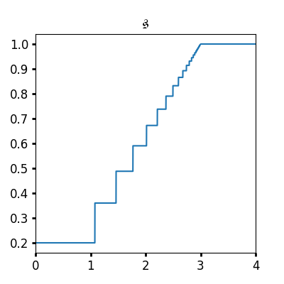
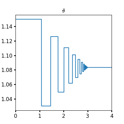
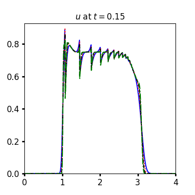
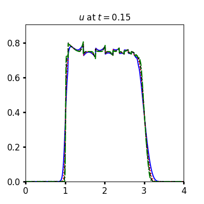
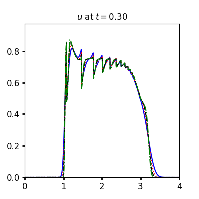
(a) $\displaystyle f(u)=u$, monotone $\displaystyle\mathfrak{s}$

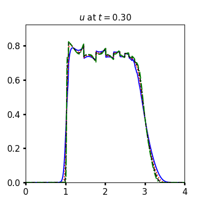
(b) $\displaystyle f(u)=u(1-u)$, non-monotone $\displaystyle\mathfrak{s}$

Figure 1: Solution to (1.8)-(1.9) on the domain $\displaystyle[0,\,4]$ at times $\displaystyle t=0.00,\;0.15,\;0.30$ with decreasing mesh size $\displaystyle\Delta x=1/75$( ), $\displaystyle\Delta x=1/150$( ), $\displaystyle\Delta x=1/300$( ) and $\displaystyle\Delta x=1/600$( )

We present some numerical experiments to illustrate the theory presented in the previous sections. We show the results for (3.3) with Lax–Friedrichs type flux. The results obtained by (3.3) with Godunov type flux are similar, and are not shown here. Throughout the section, $\displaystyle\Theta$ is chosen to be $\displaystyle 1/3$, and $\displaystyle\lambda$ is chosen so as to satisfy the CFL condition (3.4). We consider the (1.8)-(1.9) with the kernel

$$\displaystyle\mu(x) \displaystyle=L(\varepsilon^{2}-x^{2})^{3}\mathbbm{1}_{(-\varepsilon,\varepsilon)}(x),\,x\in\mathbb{R},$$

$\displaystyle L$ being such that $\displaystyle\int_{\mathbb{R}}\mu(x)\mathinner{\mathrm{d}{x}}=1,$ the velocity $\displaystyle\nu(a)=1-a,$ and with

$$\displaystyle\quad\mathfrak{s}(x)=\begin{cases}\frac{1}{3}a_{1},\quad&x\leq a_{1},\\ \frac{1}{3}\sum\limits_{n=2}^{\infty}a_{n}\mathbbm{1}_{[a_{n},a_{n+1}]}(x),\quad&x\in(a_{1},3],\\ 1,\quad&x>3,\\ \end{cases},$$

admitting infinitely many

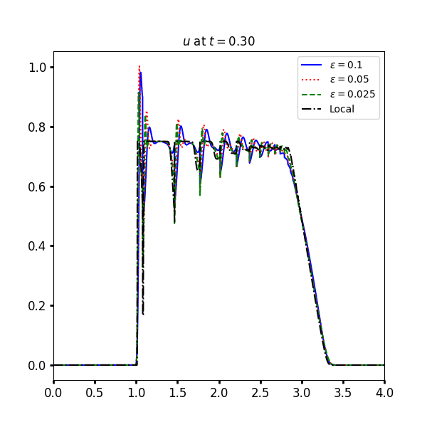
$\displaystyle\varepsilon$	$\displaystyle 0.1$	$\displaystyle 0.05$	$\displaystyle 0.0.025$	$\displaystyle 0.01$
$\displaystyle e_{\varepsilon}$	$\displaystyle 0.1031$	$\displaystyle 0.0685$	$\displaystyle 0.0390$	$\displaystyle 0.0257$

Figure 2: $\displaystyle L^{1}$ difference between Nonlocal solution of (1.8)-(1.9) with decreasing kernel support $\displaystyle\varepsilon$ and corresponding local solution, $\displaystyle\Delta x=1/600,T=0.3$: linear $\displaystyle f$, and increasing $\displaystyle\mathfrak{s}$

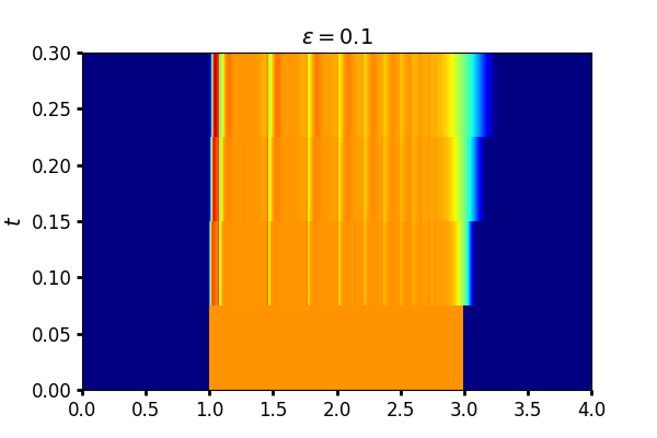
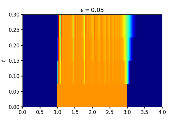
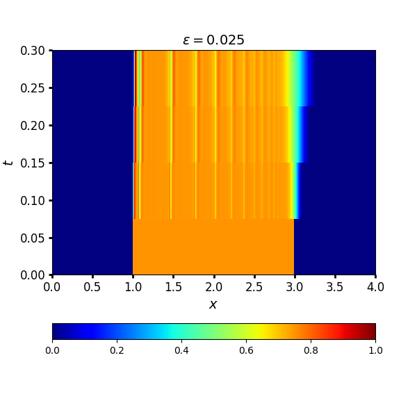
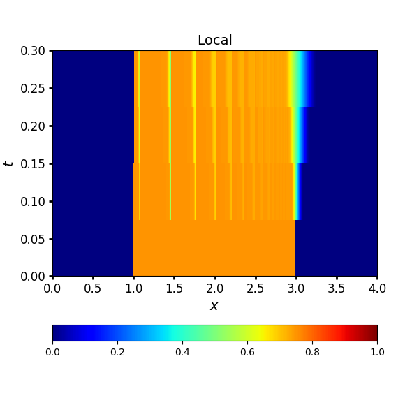
Figure 3: Nonlocal solution of (1.8)-(1.9) with decreasing kernel support $\displaystyle\varepsilon$ and corresponding local solution, $\displaystyle\Delta x=1/600,t\in[0,0.3]$: linear $\displaystyle f$, and increasing $\displaystyle\mathfrak{s}$

discontinuities at the points $\displaystyle\{a_{n}\}_{n\in\mathbb{N}},$ with

1. $\displaystyle a_{n}=3(1-0.8^{n})$ making $\displaystyle\mathfrak{s}$ non–decreasing

2. $\displaystyle a_{n}=(1-(-0.8)^{n})/12+1$ making $\displaystyle\mathfrak{s}$ non–monotonic.

We also present numerical integration with two choices of local part of the fluxes namely, $\displaystyle f(u)=u$ and $\displaystyle f(u)=u(1-u)$. All the parameters described above fit in the hypothesis of the paper. We choose the domain $\displaystyle[0,\,4]$ and the time interval $\displaystyle[0,\,0.3]$ with initial data

$$u_{0}(x)=0.75\mathbbm{1}_{(1,3)}(x).$$

Figure 1 displays the numerical approximations generated by the numerical scheme (3.3), with decreasing grid size $\displaystyle\Delta x$, starting with $\displaystyle\Delta x=1/75$ for various combinations of the above parameters at times $\displaystyle t=0.15$ and $\displaystyle t=0.30$.

Figure 1(a) represents the behavior of the solutions with monotonic $\displaystyle\mathfrak{s}$ and with linear $\displaystyle f(u)=u.$ It can be seen that the density $\displaystyle u$ goes beyond $\displaystyle 0.75$ violating the invariant region principle, a phenomenon also observed in non-local conservation laws with smooth local part, see [9].

Figure 1(b) represents the behavior of the solutions with non-monotonic $\displaystyle\mathfrak{s}$ and with non-linear $\displaystyle f(u)=u(1-u),$ with zeros at $\displaystyle u=0$ and $\displaystyle u=1.$ It can be seen that the density $\displaystyle u$ always lies within the interval $\displaystyle[0,1]$ demonstrating the invariant region principle (see Lemma 3.5).

It can be seen that the numerical scheme is able to capture the features of the solutions well. The roughness of the coefficient $\displaystyle\mathfrak{s}$ leads to the abruptness in the entropy solution which can be seen along the discontinuities of $\displaystyle\mathfrak{s}$. The results of other combinations of parameters(non-monotone $\displaystyle\mathfrak{s}$ with linear $\displaystyle f$, and non-linear $\displaystyle f$ with monotone $\displaystyle\mathfrak{s}$), are similar and not shown here.

Figures 2-3 investigate the behavior of the approximate solutions as the kernel support $\displaystyle\varepsilon\rightarrow 0.$ For this experiment, we choose monotonic $\displaystyle\mathfrak{s}$ with $\displaystyle f(u)=u.$ With $\displaystyle\Delta x=1/600,$ we compare the nonlocal solution $\displaystyle{u^{\Delta}_{\varepsilon}}$ obtained by (3.3) with the Lax-Friedrichs type flux with $\displaystyle{u^{\Delta}_{loc}}$, the solution for the corresponding local conservation law (1.8)-(1.9) obtained using the local Godunov scheme of [42] at time $\displaystyle T=0.3$, as $\displaystyle\varepsilon$ takes values $\displaystyle 0.1,0.05$, $\displaystyle 0.025$ and $\displaystyle 0.01$.

Let $\displaystyle e_{\varepsilon}:={{\left\|u^{\Delta}_{loc}(0.3,\cdot)-u^{\Delta}_{\varepsilon}(0.3,\cdot)\right\|}_{L^{1}(\mathbb{R})}}.$ It can be seen in Figure 2 that $\displaystyle e_{\varepsilon}$ decreases as $\displaystyle\varepsilon\rightarrow 0^{+}$ and that the non-local approximations seem to converge to local solution with decreasing $\displaystyle\varepsilon.$ The findings of the experiment suggest that one can possibly obtain the solutions of the local conservation laws, by decreasing the kernel support, and is a question of independent interest.

References

• [1] Adimurthi, S. S. Ghoshal, R. Dutta, and G. Veerappa Gowda. Existence and nonexistence of TV bounds for scalar conservation laws with discontinuous flux. Comm. Pure Appl. Math., 64(1):84–115, 2011.
• [2] Adimurthi, J. Jaffré, and G. D. Veerappa Gowda. Godunov-type methods for conservation laws with a flux function discontinuous in space. SIAM J. Numer. Anal., 42(1):179–208, 2004.
• [3] Adimurthi, S. Mishra, and G. D. Veerappa Gowda. Optimal entropy solutions for conservation laws with discontinuous flux-functions. J. Hyperbolic Differ. Equ., 2(04):783–837, 2005.
• [4] A. Aggarwal, R. M. Colombo, and P. Goatin. Nonlocal systems of conservation laws in several space dimensions. SIAM J. Numer. Anal., 53(2):963–983, 2015.
• [5] A. Aggarwal and P. Goatin. Crowd dynamics through non-local conservation laws. Bull. Braz. Math. Soc. (N.S.), 47(1):37–50, 2016.
• [6] A. Aggarwal, H. Holden, and G. Vaidya. On the accuracy of the finite volume approximations to nonlocal conservation laws. arXiv:2306.00142, 2023.
• [7] A. Aggarwal, M. R. Sahoo, A. Sen, and G. Vaidya. Solutions with concentration for conservation laws with discontinuous flux and its applications to numerical schemes for hyperbolic systems. Stud. Appl. Math., 145(2):247–290, 2020.
• [8] D. Amadori and W. Shen. An integro-differential conservation law arising in a model of granular flow. J. Hyperbolic Differ. Equ., 9(1):105–131, 2012.
• [9] P. Amorim, R. M. Colombo, and A. Teixeira. On the numerical integration of scalar nonlocal conservation laws. ESAIM Math. Model. Numer. Anal., 49(1):19–37, 2015.
• [10] B. Andreianov, K. H. Karlsen, and N. H. Risebro. $\displaystyle L^{1}$ stability for entropy solutions of nonlinear degenerate parabolic convection-diffusion equations with discontinuous coefficients. Netw. Heterog. Media, 5(3):617–633, 2010.
• [11] B. Andreianov, K. H. Karlsen, and N. H. Risebro. A theory of $\displaystyle L^{1}$-dissipative solvers for scalar conservation laws with discontinuous flux. Arch. Ration. Mech. Anal., 201(1):27–86, 2011.
• [12] E. Audusse and B. Perthame. Uniqueness for scalar conservation laws with discontinuous flux via adapted entropies. Proc. Roy. Soc. Edinburgh A, 135(2):253–266, 2005.
• [13] F. Betancourt, R. Bürger, K. H. Karlsen, and E. M. Tory. On nonlocal conservation laws modelling sedimentation. Nonlinearity, 24(3):855, 2011.
• [14] S. Blandin and P. Goatin. Well-posedness of a conservation law with non-local flux arising in traffic flow modeling. Numer. Math., 132(2):217–241, 2016.
• [15] A. Bressan and W. Shen. On traffic flow with nonlocal flux: a relaxation representation. Arch. Ration. Mech. Anal., 237(3):1213–1236, 2020.
• [16] A. Bressan and W. Shen. Entropy admissibility of the limit solution for a nonlocal model of traffic flow. Commun. Math. Sci., 19(5):1447–1450, 2021.
• [17] R. Bürger, H. D. Contreras, L. M. Villada, R. Bürger, H. D. Contreras, and L. M. Villada. A Hilliges-Weidlich-type scheme for a one-dimensional scalar conservation law with nonlocal flux. Netw. Heterog. Media, 18(2):664–693, 2023.
• [18] R. Bürger, A. García, K. H. Karlsen, and J. D. Towers. A family of numerical schemes for kinematic flows with discontinuous flux. J. Engrg. Math., 60(3):387–425, 2008.
• [19] R. Bürger, K. H. Karlsen, and J. D. Towers. An Engquist-Osher-type scheme for Conservation Laws with Discontinuous Flux Adapted to Flux Connections. SIAM J. Numer. Anal., 47(3):1684–1712, 2009.
• [20] F. A. Chiarello and G. M. Coclite. Non-local scalar conservation laws with discontinuous flux. Netw. Heterog. Media, 18(1):380–398, 2022.
• [21] F. A. Chiarello and L. M. Villada. On existence of entropy solutions for 1d nonlocal conservation laws with space discontinuous flux. arXiv:2103.13362, 2021.
• [22] G. M. Coclite, J.-M. Coron, N. De Nitti, A. Keimer, and L. Pflug. A general result on the approximation of local conservation laws by nonlocal conservation laws: The singular limit problem for exponential kernels. Ann. Inst. H. Poincaré C Anal. Non Linéaire, 2022.
• [23] G. M. Coclite, N. De Nitti, A. Keimer, and L. Pflug. Singular limits with vanishing viscosity for nonlocal conservation laws. Nonlinear Anal., 211:112370, 2021.
• [24] G. M. Coclite, K. H. Karlsen, and N. H. Risebro. A nonlocal lagrangian traffic flow model and the zero-filter limit. arXiv:2302.03889, 2023.
• [25] M. Colombo, G. Crippa, E. Marconi, and L. V. Spinolo. Local limit of nonlocal traffic models: convergence results and total variation blow-up. Ann. Inst. H. Poincaré C Anal. Non Linéaire, 38(5):1653–1666, 2021.
• [26] M. Colombo, G. Crippa, E. Marconi, and L. V. Spinolo. Nonlocal Traffic Models with General Kernels: Singular Limit, Entropy Admissibility, and Convergence Rate. Arch. Ration. Mech. Anal., 247(2):18, 2023.
• [27] M. Colombo, G. Crippa, and L. V. Spinolo. On the singular local limit for conservation laws with nonlocal fluxes. Arch. Ration. Mech. Anal., 233(3):1131–1167, 2019.
• [28] R. M. Colombo, M. Garavello, and M. Lécureux-Mercier. A class of nonlocal models for pedestrian traffic. Math. Mod. Met. Appl. Sci., 22(4):1150023–34, 2012.
• [29] R. M. Colombo, M. Herty, and M. Lécureux-Mercier. Control of the continuity equation with a non local flow. ESAIM Control Optim. Calc. Var., 17(2):353–379, 2011.
• [30] R. M. Colombo, M. Herty, and M. Mercier. Control of the continuity equation with a non local flow. ESAIM Control Optim. Calc. Var., 17(2):353–379, 2011.
• [31] R. M. Colombo and M. Lécureux-Mercier. Nonlocal crowd dynamics models for several populations. Acta Math. Sci. Ser. B, 32(1):177–196, 2011.
• [32] R. M. Colombo and F. Marcellini. Nonlocal systems of balance laws in several space dimensions with applications to laser technology. J. Differential Equations, 259(11):6749–6773, 2015.
• [33] J.-M. Coron, A. Keimer, and L. Pflug. Nonlocal transport equations-existence and uniqueness of solutions and relation to the corresponding conservation laws. SIAM J. Math. Anal., 52(6):5500–5532, 2020.
• [34] J. Friedrich, S. Göttlich, A. Keimer, and L. Pflug. Conservation laws with nonlocal velocity–the singular limit problem. arXiv:2210.12141, 2022.
• [35] J. Friedrich, S. Göttlich, A. Keimer, and L. Pflug. Conservation laws with nonlocality in density and velocity and their applicability in traffic flow modelling. arXiv:2302.12797, 2023.
• [36] J. Friedrich, O. Kolb, and S. Göttlich. A Godunov type scheme for a class of LWR traffic flow models with non-local flux. Netw. Heterog. Media, 13(4):531–547, 2018.
• [37] M. Garavello, R. Natalini, B. Piccoli, and A. Terracina. Conservation laws with discontinuous flux. Netw. Heterog. Media, 2(1):159, 2007.
• [38] S. S. Ghoshal. Optimal results on TV bounds for scalar conservation laws with discontinuous flux. J. Differential Equations, 258(3):980–1014, 2015.
• [39] S. S. Ghoshal, A. Jana, and J. D. Towers. Convergence of a Godunov scheme to an Audusse–Perthame adapted entropy solution for conservation laws with BV spatial flux. Numer. Math., 146(3):629–659, 2020.
• [40] S. S. Ghoshal, J. D. Towers, and G. Vaidya. Well-posedness for conservation laws with spatial heterogeneities and a study of BV regularity. arXiv:2010.13695, 2020.
• [41] S. S. Ghoshal, J. D. Towers, and G. Vaidya. Convergence of a Godunov scheme for degenerate conservation laws with BV spatial flux and a study of Panov-type fluxes. J. Hyperbolic Differ. Equ., 19(02):365–390, 2022.
• [42] S. S. Ghoshal, J. D. Towers, and G. Vaidya. A Godunov type scheme and error estimates for scalar conservation laws with Panov-type discontinuous flux. Numer. Math., 151:601–625, 2022.
• [43] P. Goatin and E. Rossi. Well-posedness of IBVP for 1D scalar non-local conservation laws. Z. Angew. Math. Mech., 99(11):e201800318, 2019.
• [44] S. Göttlich, S. Hoher, P. Schindler, V. Schleper, and A. Verl. Modeling, simulation and validation of material flow on conveyor belts. Appl. Math. Model., 38(13):3295–3313, 2014.
• [45] H. Holden and N. H. Risebro. Front Tracking for Hyperbolic Conservation Laws. Springer, second edition, 2015.
• [46] K. H. Karlsen and N. H. Risebro. On the uniqueness and stability of entropy solutions of nonlinear degenerate parabolic equations with rough coefficients. Discrete Contin. Dyn. Syst., 9(5):1081, 2003.
• [47] A. Keimer and L. Pflug. Existence, uniqueness and regularity results on nonlocal balance laws. J. Differential Equations, 263(7):4023–4069, 2017.
• [48] A. Keimer and L. Pflug. On approximation of local conservation laws by nonlocal conservation laws. J. Math. Anal. Appl., 475(2):1927–1955, 2019.
• [49] A. Keimer and L. Pflug. Discontinuous nonlocal conservation laws and related discontinuous ODEs—existence, uniqueness, stability and regularity. 2110.10503, 2021.
• [50] A. Keimer and L. Pflug. On the singular limit problem for a discontinuous nonlocal conservation law. arXiv:2212.12598, 2022.
• [51] A. Keimer and L. Pflug. On the singular limit problem for a discontinuous nonlocal conservation law. arXiv:2212.12598, 2022.
• [52] A. Keimer, L. Pflug, and M. Spinola. Nonlocal scalar conservation laws on bounded domains and applications in traffic flow. SIAM J. Math. Anal., 50(6):6271–6306, 2018.
• [53] Y. Lee. Thresholds for shock formation in traffic flow models with nonlocal-concave-convex flux. J. Differ. Equations, 266(1):580–599, 2019.
• [54] E. Y. Panov. On existence and uniqueness of entropy solutions to the Cauchy problem for a conservation law with discontinuous flux. J. Hyperbolic Differ. Equ., 6(03):525–548, 2009.
• [55] B. Perthame. Transport Equations in Biology. Frontiers in Mathematics. Birkhäuser, 2007.
• [56] J. D. Towers. An existence result for conservation laws having BV spatial flux heterogeneities — without concavity. J. Differential Equations, 269(7):5754–5764, 2020.