A High–Order Perturbation of Envelopes (HOPE) Method for Vector Electromagnetic Scattering by Periodic Inhomogeneous Media

Abstract

The scattering of electromagnetic waves by three–dimensional periodic structures is important for many problems of crucial scientific and engineering interest. Due to the complexity and three–dimensional nature of these waves, the fast, accurate, and reliable numerical simulations of these are indispensable for engineers and scientists alike. For this, High–Order Spectral methods are frequently employed and here we describe an algorithm in this class. Our approach is perturbative in nature where we view the deviation of the permittivity from a constant value as the deformation and we pursue regular perturbation theory. This work extends our previous contribution regarding the Helmholtz equation to the full vector Maxwell equations, by providing a rigorous analyticity theory, both in deformation size and spatial variable (provided that the permittivity is, itself, analytic).

1 Introduction

The scattering of electromagnetic waves by three–dimensional periodic structures is important for many problems of crucial scientific and engineering interest. Examples abound in areas as disparate as surface enhanced spectroscopy [21], extraordinary optical transmission [5], cancer therapy [6], and surface plasmon resonance (SPR) biosensing [13, 16, 19, 25].

Due to their central role in these nanotechnologies, simulations of these waves have been conducted with all of the classical numerical algorithms for approximating solutions to the relevant governing partial differential equations. This includes the Finite Difference [30, 18], Finite Element [15, 14], Discontinuous Galerkin [12], Spectral Element [4], and Spectral [11, 28, 29] methods. While these are tempting choices, due to their volumetric nature they require a large number of unknowns ($N=N_{x}N_{y}N_{z}$ for a three–dimensional simulation) and mandate the inversion of large, non–symmetric positive definite matrices (of dimension $N\times N$). Such properties are still an object of current study (for instance, see [7, 20]).

For the specific application of SPR sensors which we have in mind in the current contribution, their pervasiveness stems from two properties of an SPR, namely its extremely strong and sensitive response. More specifically, over the range of tens of nanometers in incident wavelength, the reflected energy can fall from nearly 100 % by a factor of 10 or even 100 before returning to almost 100 %. Obviously, to approximate such a structure with the required accuracy, the numerical algorithm should produce high fidelity results in a rapid and robust manner. For this reason we will focus upon High–Order Spectral (HOS) methods [11, 28, 29] which can deliver precisely this behavior.

Returning to the classical approaches listed above, for the problem of scattering by homogeneous layers (which is one important avenue to generating SPRs) it is clearly unnecessary to discretize the bulk of each layer and state–of–the–art solvers seek interfacial unknowns with the knowledge that information inside the layers can readily be computed from appropriate integral formulas. Boundary element (BEM) [27] and boundary integral (BIM) [3, 17] methods are two such approaches and can produce spectrally accurate solutions in a fraction of the time of their volumetric competitors.

In previous work [22] the authors investigated a novel algorithm very much in the spirit of these HOS approaches, and inspired by the “High–Order Perturbation of Surfaces” (HOPS) algorithms which have proven to be so appealing for layered media. A HOPS scheme is one which views the layer interfaces as perturbations of flat ones and then makes recursive corrections to the scattering returns from this classical, exactly solvable, configuration [31]. By contrast, our new “High–Order Perturbation of Envelopes” (HOPE) scheme considers more a general permittivity function, $\epsilon(x,y,z)$, which does not necessarily have layered structure. We followed the lead of Feng, Lin, and Lorton [9, 10] and adopted a perturbative philosophy (much like a HOPS algorithm) by viewing the permittivity as a perturbation of a trivial one, e.g.,

$$\epsilon(x,y,z)=\bar{\epsilon}-\delta\mathcal{E}(x,y,z),\quad\bar{\epsilon}\in\mbox{${\bf R}$},\quad\mathcal{E}(x+d_{x},y+d_{y},z)=\mathcal{E}(x,y,z),$$

where $\mathcal{E}$ is a permittivity “envelope.” In this previous contribution we focused upon the two–dimensional scalar problems governing electromagnetic radiation in Transverse Electric (TE) and Transverse Magnetic (TM) polarizations. This new approach has computational advantages over volumetric solvers in certain configurations (e.g., where the support of $\mathcal{E}$ is small or where the set on which $\mathcal{E}$ significantly changes is small). A particular choice we pursued was an approximate indicator function which is nearly zero/unity to denote the absence/presence of a material.

Among the contributions of [22] was a new, extensive, and rigorous analysis. More specifically, we proved not only that the domain of analyticity of the scattered field in $\delta$ can be extended to a neighborhood of the entire real axis (up to topological obstruction), but also that this field is jointly analytic in parametric and spatial variables provided that $\mathcal{E}(x,y,z)$ is spatially analytic. In the current paper we extend some of these results to the three–dimensional vector electromagnetic case governed by the full time–harmonic Maxwell equations. More specifically, we show that the scattered field is analytic as a function of $\delta$ and jointly analytic in both parametric and spatial variables if $\mathcal{E}(x,y,z)$ is spatially analytic. We delay for future consideration the issue of the analytic continuation of our results to perturbations $\delta$ of arbitrary (real) size. This requires an analysis of the variable coefficient Maxwell equations [2] which is more subtle than what we present here, however, we believe that this is a result which can be established with our current framework.

The rest of the paper is organized as follows. In § 2 we recall the governing equations complete with a discussion of transparent boundary conditions in § 3. We describe the HOPE algorithm in § 4 and begin our theoretical developments with a description of the relevant function spaces in § 5. We state and prove our results on parametric analyticity in § 6 and joint parametric/spatial analyticity in § 7. In Appendix A we prove our new elliptic estimate, and in Appendix B we establish the joint analyticity result in the special case of lateral smoothness.

2 Governing Equations

We consider materials modeled by the time–harmonic Maxwell equations in three dimensions with a constant permeability $\mu=\mu_{0}$ and no currents or sources,

(2.1) $$\text{curl}\left[E\right]-i\omega\mu_{0}H=0,\quad\text{curl}\left[H\right]+i\omega\epsilon E=0,$$

where $(E,H)$ are the electric and magnetic vector fields, and we have factored out time dependence of the form $\exp(-i\omega t)$ [2]. The permittivity $\epsilon(x,y,z)$ is biperiodic with periods $d_{x}$ and $d_{y}$, and is specified by

$$\epsilon(x,y,x)=\begin{cases}\epsilon^{(u)},&z>h,\\ \epsilon^{(v)}(x,y,z),&-h<z<h,\\ \epsilon^{(w)},&z<-h,\end{cases}$$

where $\epsilon^{(u)},\epsilon^{(w)}\in\mbox{${\bf R}$}^{+}$, and $\epsilon^{(v)}(x+d_{x},y+d_{y},z)=\epsilon^{(v)}(x,y,z)$, and

$$\lim_{z\rightarrow h-}\epsilon^{(v)}(x,y,z)=\epsilon^{(u)},\quad\lim_{z\rightarrow(-h)+}\epsilon^{(v)}(x,y,z)=\epsilon^{(w)}.$$

Using the permittivity of vacuum, $\epsilon_{0}$, we can define

$$k^{2}_{0}=\omega^{2}\epsilon_{0}\mu_{0}=\frac{\omega^{2}}{c_{0}^{2}},\quad(k^{(m)})^{2}=\epsilon^{(m)}k^{2}_{0},\quad m\in\{u,w\},$$

and $c_{0}=1/\sqrt{\epsilon_{0}\mu_{0}}$ is the speed of light in the vacuum.

This structure is illuminated from above by plane–wave incident radiation of the form

$$E^{\text{inc}}(x,y,z) =A\exp(i\alpha x+i\beta y-i\gamma^{(u)}z),$$

$$H^{\text{inc}}(x,y,z) =B\exp(i\alpha x+i\beta y-i\gamma^{(u)}z),$$

where

$$A\cdot\kappa=0,\quad B=\frac{1}{\omega\mu_{0}}\kappa\times A,\quad\left|A\right|=\left|B\right|=1,$$

and

$$\kappa=\begin{pmatrix}\alpha\\ \beta\\ -\gamma^{(u)}\end{pmatrix}=k^{(u)}\begin{pmatrix}\sin(\theta)\cos(\phi)\\ \sin(\theta)\sin(\phi)\\ -\cos(\theta)\end{pmatrix},$$

where $(\theta,\phi)$ are the angles of incidence.

3 Transparent Boundary Conditions

Following our previous work [22] we aim to both rigorously specify the appropriate far–field boundary conditions and reduce the infinite domain to one of finite size. Conveniently, a variant of the scheme presented in Bao & Li [2] accomplishes both. In the upper domain $\{z>h\}$ we seek a solution as the sum of the incident radiation and an upward propagating (reflected) component, e.g.,

$$E =E^{\text{inc}}+E^{\text{refl}}$$

$$=A\exp(i\alpha x+i\beta y-i\gamma^{(u)}z)+c_{0,0}\exp(i\alpha x+i\beta y+i\gamma^{(u)}(z-h))$$

$$\quad+\sum_{(p,q)\neq(0,0)}\hat{u}_{p,q}\exp(i\alpha_{p}x+i\beta_{q}y+i\gamma^{(u)}_{p,q}(z-h)),$$

[26, 31] where

$$\alpha_{p}=\alpha+(2\pi/d_{x})p,\quad\beta_{q}=\beta+(2\pi/d_{y})q,$$

$${\gamma^{(m)}_{p,q}:=\begin{cases}\sqrt{\epsilon^{(m)}k_{0}^{2}-\alpha_{p}^{2}-\beta_{q}^{2}},&\alpha_{p}^{2}+\beta_{q}^{2}\leq\epsilon^{(m)}k_{0}^{2},\\ i\sqrt{\alpha_{p}^{2}+\beta_{q}^{2}-\epsilon^{(m)}k_{0}^{2}},&\alpha_{p}^{2}+\beta_{q}^{2}>\epsilon^{(m)}k_{0}^{2},\end{cases}}\quad m\in\{u,w\}.$$

If we set $c_{0,0}=\hat{u}_{0,0}-A\exp(-i\gamma^{(u)}h)$, implying $\hat{u}_{0,0}=c_{0,0}+A\exp(-i\gamma^{(u)}h)$, then

$$E =A\exp(i\alpha x+i\beta y-i\gamma^{(u)}z)-A\exp(i\alpha x+i\beta y+i\gamma^{(u)}(z-2h))$$

$$\quad+\sum_{p=-\infty}^{\infty}\sum_{q=-\infty}^{\infty}\hat{u}_{p,q}\exp(i\alpha_{p}x+i\beta_{q}y+i\gamma^{(u)}_{p,q}(z-h)),$$

and $E(x,y,h)=u(x,y)$. It is a simple matter to show that

$$\partial_{z}E =(-i\gamma^{(u)})A\exp(i\alpha x+i\beta y-i\gamma^{(u)}z)$$

$$\quad-(i\gamma^{(u)})A\exp(i\alpha x+i\beta y+i\gamma^{(u)}(z-2h))$$

$$\quad+\sum_{p=-\infty}^{\infty}\sum_{q=-\infty}^{\infty}(i\gamma^{(u)}_{p,q})\hat{u}_{p,q}\exp(i\alpha_{p}x+i\beta_{q}y+i\gamma^{(u)}_{p,q}(z-h)),$$

so that

$$-\partial_{z}E(x,y,h) =(i\gamma^{(u)})A\exp(i\alpha x+i\beta y-i\gamma^{(u)}h)$$

$$\quad+(i\gamma^{(u)})A\exp(i\alpha x+i\beta y+i\gamma^{(u)}(-h))$$

$$\quad+\sum_{p=-\infty}^{\infty}\sum_{q=-\infty}^{\infty}(-i\gamma^{(u)}_{p,q})\hat{u}_{p,q}\exp(i\alpha_{p}x+i\beta_{q}y).$$

If we define the function

(3.1) $$\phi(x,y):=\left(2i\gamma^{(u)}\exp(-i\gamma^{(u)}h)\right)A\exp(i\alpha x+i\beta y),$$

and the order–one Fourier multiplier (the externally directed Dirichlet–Neumann operator for the Maxwell equation on $\{z>h\}$)

$$T_{u}[\psi]:=\sum_{p=-\infty}^{\infty}\sum_{q=-\infty}^{\infty}(-i\gamma^{(u)}_{p,q})\hat{\psi}_{p,q}\exp(i\alpha_{p}x+i\beta_{q}y),$$

then we see that we can express the Upward Propagating Condition (UPC) [1] exactly with the boundary condition

$$-\partial_{z}E(x,y,h)-T_{u}[E(x,y,h)]=\phi(x,y).$$

In a similar fashion, in $\{z<-h\}$ we seek a solution which is purely downward propagating (transmitted)

$$E=E^{\text{trans}}=\sum_{p=-\infty}^{\infty}\sum_{q=-\infty}^{\infty}\hat{w}_{p,q}\exp(i\alpha_{p}x+i\beta_{q}y-i\gamma^{(w)}_{p,q}(z+h)),$$

[26, 31]. Clearly $E(x,y,-h)=w(x,y)$ and, with the calculation

$$\partial_{z}E(x,y,-h)=\sum_{p=-\infty}^{\infty}\sum_{q=-\infty}^{\infty}(-i\gamma^{(w)}_{p,q})\hat{w}_{p,q}\exp(i\alpha_{p}x+i\beta_{q}y),$$

and the analogous order–one Fourier multiplier (again, the externally directed Dirichlet–Neumann operator for the Helmholtz equation on $\{z<-h\}$)

$$T_{w}[\psi]:=\sum_{p=-\infty}^{\infty}\sum_{q=-\infty}^{\infty}(-i\gamma^{(w)}_{p,q})\hat{\psi}_{p,q}\exp(i\alpha_{p}x+i\beta_{q}y),$$

we can state the Downward Propagating Condition (DPC) [1] transparently using

$$\partial_{z}E(x,y,-h)-T_{w}[E(x,y,-h)]=0.$$

Eliminating the magnetic field from (2.1) and gathering our full set of governing equations we find the following problem to solve.

(3.2a) $$\text{curl}\left[\text{curl}\left[E\right]\right]-\epsilon^{(v)}k_{0}^{2}E=0, \text{in $S_{v}$},$$

(3.2b) $$-\partial_{z}E-T_{u}[E]=\phi, \text{at $\Gamma_{h}$},$$

(3.2c) $$\partial_{z}E-T_{w}[E]=0, \text{at $\Gamma_{-h}$},$$

(3.2d) $$E(x+d_{x},y+d_{y},z)=\exp(i\alpha d_{x}+i\beta d_{y})E(x,y,z),$$

where

$$S_{v}:=(0,d_{x})\times(0,d_{y})\times(-h,h),\quad\Gamma_{\pm h}:=(0,d_{x})\times(0,d_{y})\times\{z=\pm h\}.$$

4 A High–Order Perturbation of Envelopes Method

Following the lead of our previous work [22] we do not pursue the solution of (3.2) by a classical volumetric approach, but rather a perturbative one where we think of our configuration as a small deviation from a trivial structure,

$$\epsilon^{(v)}(x,y,z)=\bar{\epsilon}\left(1-\delta\mathcal{E}(x,y,z)\right)=\bar{\epsilon}-\delta(\bar{\epsilon}\mathcal{E}(x,y,z)),$$

where $\bar{\epsilon}\in\mbox{${\bf R}$}^{+}$ is a constant, and $\delta\ll 1$. In our previous work on the Helmholtz equation in either TE or TM polarization, we showed that if $\mathcal{E}(x,z)$ is smooth enough then the transverse components of $E$ or $H$ depend analytically upon $\delta$. In light of this we posit that, for the full Maxwell equations which we consider here, the field $E=E(x,y,z;\delta)$ depends analytically upon $\delta$ so that

(4.1) $$E=E(x,y,z;\delta)=\sum_{\ell=0}^{\infty}E_{\ell}(x,y,z)\delta^{\ell},$$

converges strongly in a function space. It is not difficult to see that these $E_{\ell}$ must satisfy

(4.2a) $$\text{curl}\left[\text{curl}\left[E_{\ell}\right]\right]-\bar{\epsilon}k_{0}^{2}E_{\ell}=\bar{\epsilon}k_{0}^{2}\mathcal{E}E_{\ell-1}, \text{in $S_{v}$},$$

(4.2b) $$-\partial_{z}E_{\ell}-T_{u}[E_{\ell}]=\delta_{\ell,0}\phi, \text{at $\Gamma_{h}$},$$

(4.2c) $$\partial_{z}E_{\ell}-T_{w}[E_{\ell}]=0, \text{at $\Gamma_{-h}$},$$

(4.2d) $$E_{\ell}(x+d_{x},y+d_{y},z)=\exp(i\alpha d_{x}+i\beta d_{y})E_{\ell}(x,y,z),$$

where $\delta_{\ell,0}$ is the Kronecker delta function. It is easy to see that

(4.3) $$E_{0}(x,y,z)=Ae^{i\alpha x+i\beta y-i\bar{\gamma}z},\quad\alpha^{2}+\beta^{2}+(\bar{\gamma})^{2}=\bar{\epsilon}k_{0}^{2},$$

and our HOPE scheme can be viewed as computing corrections to this by

$$E(x,y,z)=Ae^{i\alpha x+i\beta y-i\bar{\gamma}z}+\sum_{\ell=1}^{\infty}E_{\ell}(x,y,z)\delta^{\ell}.$$

We note that a natural numerical method would seek approximations of the $E_{\ell}$ for $1\leq\ell\leq L$ and simulate

$$E(x,y,z;\delta)\approx E^{L}(x,y,z;\delta):=\sum_{\ell=0}^{L}E_{\ell}(x,y,z)\delta^{\ell}.$$

There are many possibilities for the envelope function $\mathcal{E}(x,y,z)$ and each leads to a slightly different perturbation approach. For instance, consider the function

$$\Phi_{a,b}(z):=\frac{\tanh(w(z-a))-\tanh(w(z-b))}{2},$$

with sharpness parameter $w$, which is effectively zero outside the interval $(a,b)$ while being essentially one inside $(a,b)$, c.f. [22]. We can approximate a slab of material with thickness $2d$ and a gap of width $2g$ in vacuum by selecting

$$\bar{\epsilon}=1,\quad\mathcal{E}(x,y,z)=\Phi_{-d,d}(z)\left\{1-\Phi_{-g,g}(x)\right\},\quad\delta=1.$$

See Figure 1 with the choices $d=1/4$, $g=1/10$, and $w=50$ on the cell $[-1,1]\times[-1,1]$.

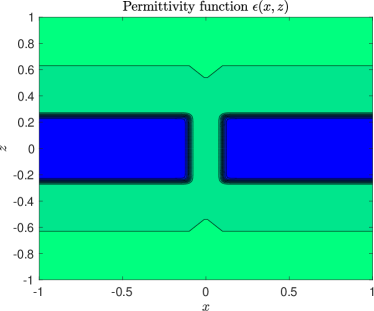
Fig. 1: Contour plots of $\mathcal{E}(x,z)$ (left) and $\epsilon^{(v)}(x,z)$ (right).

5 Function spaces

In this section, we present function spaces and theoretical notions that are necessary for our analysis later. We point out that due to the vectorial nature of the Maxwell equations, these are extensions of the results we utilized in our previous study [22]. For any real number $s\geq 0$, we have the classical interfacial quasiperiodic $L^{2}$ Sobolev norm

$$\left\|v\right\|_{H^{s}}^{2}:=\sum_{p=-\infty}^{\infty}\sum_{q=-\infty}^{\infty}\langle(p,q)\rangle^{2s}\left|\hat{v}_{p,q}\right|^{2},$$

$$\left|\hat{v}_{p,q}\right|^{2}=\left|\hat{v}^{x}_{p,q}\right|^{2}+\left|\hat{v}^{y}_{p,q}\right|^{2}+\left|\hat{v}^{z}_{p,q}\right|^{2},$$

where

$$\langle(p,q)\rangle^{2}:=1+\left|p\right|^{2}+\left|q\right|^{2},\quad\hat{v}^{m}_{p,q}:=\frac{1}{d_{x}d_{y}}\int_{0}^{d_{x}}\int_{0}^{d_{y}}v^{m}(x,y)e^{-i\alpha_{p}x-i\beta_{q}y}\;dx\;dy,$$

for $m\in\{x,y,z\}$. From this we define the interfacial quasiperiodic Sobolev space [17]

$$H^{s}(\Gamma)=\left\{v(x,y)\in(L^{2}(\Gamma))^{3}\ |\ \left\|v\right\|_{H^{s}}<\infty\right\},$$

where

$$\Gamma:=(0,d_{x})\times(0,d_{y}).$$

In addition, we mention that the dual space of $H^{s}$, $H^{-s}$, can be defined by the norm above with a negative index. We also recall the space of $s$-times continuously differentiable functions with Hölder norm

$$\left|v\right|_{C^{s}}:=\max_{0\leq\ell+r\leq s}\max_{m\in\{x,y,z\}}\left|\partial_{x}^{\ell}\partial_{y}^{r}v^{m}\right|_{L^{\infty}}.$$

Finally, we define the volumetric laterally quasiperiodic Sobolev space as

$$H^{s}(S_{v})=\left\{u(x,y,z)\in(L^{2}(S_{v}))^{3}\ |\ \left\|u\right\|_{H^{s}}<\infty\right\},$$

where

$$\left\|u\right\|_{H^{s}}^{2}:=\sum_{j=0}^{s}\sum_{p=-\infty}^{\infty}\sum_{q=-\infty}^{\infty}\langle(p,q)\rangle^{2(s-j)}\int_{-h}^{h}\left|\partial_{z}^{j}\hat{u}_{p,q}(z)\right|^{2}\;dz.$$

We will also have need of the “H–div” space

$$H^{s}(\mbox{\rm div\,},S_{v})=\left\{u(x,y,z)\in H^{s}(S_{v})\ |\ \mbox{\rm div\,}\left[u\right]\in H^{s}(S_{v})\right\}.$$

We close with an essential result [8, 23] required for our later proofs.

Lemma 1.

Let $s\geq 0$ be an integer and $g\in C^{s}(D)$, $w\in H^{s}(D)$, where $D$ is a subset of $\mbox{${\bf R}$}^{m}$, then $gw\in H^{s}(D)$ and

$$\left\|gw\right\|_{H^{s}}\leq\tilde{M}(m,s,D)\left|g\right|_{C^{s}}\left\|w\right\|_{H^{s}},$$

where $\tilde{M}$ is some positive universal constant.

Furthermore, we recall the following elementary result [24, 22].

Lemma 2.

Let $s\geq 0$ be an integer, then there exists a constant $S>0$ such that

$$\sum_{j=0}^{s}\frac{(s+1)^{2}}{(s-j+1)^{2}(j+1)^{2}}<S,\quad\sum_{j=0}^{s}\sum_{r=0}^{j}\frac{(s+1)^{2}}{(s-j+1)^{2}(j-r+1)^{2}(r+1)^{2}}<S^{2}.$$

6 Analyticity

At this point we are in a position to extend our previous results [22] by demonstrating the analytic dependence of the full electric field, $E=E(x,y,z;\delta)$, upon $\delta$, sufficiently small. More specifically, we show that the expansion (4.1) converges strongly in an appropriate function space.

For this we require an elliptic estimate for our inductive proof which is established in Appendix A. For future convenience, we define the following differential operator associated to the Maxwell system

$$\mathcal{L}_{0}:=\mbox{\rm curl\,}\mbox{\rm curl\,}-k^{2}_{0}\bar{\epsilon}.$$

As is well known [2], the issue of uniqueness of solutions to the Maxwell problem

(6.1a) $$\mathcal{L}_{0}V=0, \text{in $S_{v}$},$$

(6.1b) $$-\partial_{z}V-T_{u}[V]=0, \text{at $\Gamma_{h}$},$$

(6.1c) $$\partial_{z}V-T_{w}[V]=0, \text{at $\Gamma_{-h}$},$$

(6.1d) $$V(x+d_{x},y+d_{y},z)=\exp(i\alpha d_{x}+i\beta d_{y})V(x,y,z),$$

c.f. (4.2), which should have only the trivial solution $V\equiv 0$, is a subtle one and certain illuminating frequencies $\omega$ will induce non–uniqueness in some configurations. Unfortunately a precise characterization of the set of forbidden frequencies is elusive and all that is known is that it is countable and accumulates at infinity [2]. To accommodate this state of affairs we define the set of permissible configurations

(6.2) $$\mathcal{P}:=\left\{(\omega,\bar{\epsilon})\ |\ V\equiv 0\ \text{is the unique solution of \eqref{Eqn:Max:Uniqueness}}\right\}.$$

With this we can now state the following fundamental elliptic regularity result.

Theorem 3.

Given any integer $s\geq 0$, if $(\omega,\bar{\epsilon})\in\mathcal{P}$, $F\in H^{s}(S_{v})\cap H^{s+1}(\mbox{\rm div\,},S_{v})$, $Q\in H^{s+1/2}(\Gamma)$, and $R\in H^{s+1/2}(\Gamma)$, then there exists a unique solution of

(6.3a) $$\mathcal{L}_{0}v=F, \text{in $S_{v}$},$$

(6.3b) $$-\partial_{z}v-T_{u}[v]=Q \text{at $\Gamma_{h}$},$$

(6.3c) $$\partial_{z}v-T_{w}[v]=R \text{at $\Gamma_{-h}$},$$

(6.3d) $$v(x+d_{x},y+d_{y},z)=e^{i\alpha d_{x}+i\beta d_{y}}v(x,y,z),$$

satisfying

(6.4) $$\left\|v\right\|_{H^{s+2}}\leq C_{e}\left(\left\|F\right\|_{H^{s}}+\left\|\mbox{\rm div\,}\left[F\right]\right\|_{H^{s+1}}+\left\|Q\right\|_{H^{s+1/2}}+\left\|R\right\|_{H^{s+1/2}}\right),$$

where $C_{e}>0$ is a universal constant.

We can now prove our analyticity result.

Theorem 4.

Given any integer $s\geq 0$, if $(\omega,\bar{\epsilon})\in\mathcal{P}$, and $\mathcal{E}\in C^{s+2}(S_{v})$ then the series (4.1) converges strongly. More precisely,

(6.5) $$\left\|E_{\ell}\right\|_{H^{s+2}}\leq KB^{\ell},\quad\forall\ \ell\geq 0,$$

for some universal constants $K,B>0$.

Proof.

We prove the estimate (6.5) by induction. For $\ell=0$ the system (4.2) can be written as

$$\mathcal{L}_{0}E_{0}=0, \text{in $S_{v}$},$$

$$-\partial_{z}E_{0}-T_{u}[E_{0}]=\phi, \text{at $\Gamma_{h}$},$$

$$\partial_{z}E_{0}-T_{w}[E_{0}]=0 \text{at $\Gamma_{-h}$},$$

$$E_{0}(x+d_{x},y+d_{y},z)=e^{i\alpha d_{x}+i\beta d_{y}}E_{0}(x,y,z).$$

So, we can apply Theorem 3 with $F\equiv 0$, $Q=\phi$, and $R\equiv 0$ to obtain

$$\left\|E_{0}\right\|_{H^{s+2}}\leq C_{e}\left\|\phi\right\|_{H^{s+1/2}}=:K.$$

Now, we assume that (6.5) is true for all $\ell<L$ and apply Theorem 3 to the system (4.2) for $E_{L}$ with $F_{L}=\bar{\epsilon}k_{0}^{2}\mathcal{E}E_{L-1}$ and $Q_{L}\equiv R_{L}\equiv 0$. This gives

$$\left\|E_{L}\right\|_{H^{s+2}} \leq C_{e}\left(\left\|\bar{\epsilon}k_{0}^{2}\mathcal{E}E_{L-1}\right\|_{H^{s}}+\left\|\mbox{\rm div\,}\left[\bar{\epsilon}k_{0}^{2}\mathcal{E}E_{L-1}\right]\right\|_{H^{s+1}}\right)$$

$$\leq C_{e}k_{0}^{2}\left|\bar{\epsilon}\right|\left\|\mathcal{E}E_{L-1}\right\|_{H^{s+2}}$$

$$\leq C_{e}k_{0}^{2}\left|\bar{\epsilon}\right|\tilde{M}\left|\mathcal{E}\right|_{C^{s+2}}\left\|E_{L-1}\right\|_{H^{s+2}}$$

$$\leq C_{e}k_{0}^{2}\left|\bar{\epsilon}\right|\tilde{M}\left|\mathcal{E}\right|_{C^{s+2}}KB^{L-1}$$

$$\leq KB^{L},$$

provided that

$$B>C_{e}k_{0}^{2}\left|\bar{\epsilon}\right|\tilde{M}\left|\mathcal{E}\right|_{C^{s+2}}.$$

∎

From this we can derive the exponential order of convergence of the HOPE method. More precisely, defining the $L$–th partial sum of (4.1)

$$E^{L}(x,y,z):=\sum_{\ell=0}^{L}E_{\ell}(x,y,z)\delta^{\ell},$$

we obtain the following error estimate for the HOPE method.

Theorem 5.

If $(\omega,\bar{\epsilon})\in\mathcal{P}$ and $E$ is the unique solution of (3.2), under the assumptions of Theorem 4 we have the estimate

$$\left\|E-E^{L}\right\|_{H^{s+2}}\lesssim(B\delta)^{L+1},$$

for some constant $B>C_{e}k_{0}^{2}\left|\bar{\epsilon}\right|\tilde{M}\left|\mathcal{E}\right|_{C^{s+2}}$ provided that $\left|\delta\right|<1/B$.

Proof.

Since

$$E(x,y,z)-E^{L}(x,y,z)=\sum_{\ell=L+1}^{\infty}E_{\ell}(x,y,z)\delta^{\ell},$$

we have, by Theorem 4,

$$\left\|E-E^{L}\right\|_{H^{s+2}}\leq\sum_{\ell=L+1}^{\infty}\left\|E_{\ell}\right\|_{H^{s+2}}\leq\sum_{\ell=L+1}^{\infty}KB^{\ell}\delta^{\ell}.$$

By gathering terms and re–indexing we have

$$\left\|E-E^{L}\right\|_{H^{s+2}}\leq K(B\delta)^{L+1}\sum_{\ell=0}^{\infty}(B\delta)^{\ell}\leq K\frac{(B\delta)^{L+1}}{1-(B\delta)},$$

for $\left|\delta B\right|<1$, where we have used the elementary fact that

$$\sum_{\ell=0}^{\infty}\alpha^{\ell}=\frac{1}{1-\alpha}$$

provided that $\left|\alpha\right|<1$. ∎

7 Joint Analyticity

We close our theoretical developments with a result on joint analyticity of the scattered field with respect to not only the perturbation parameter $\delta$, but also the spatial coordinates $(x,y,z)$. As with the analogous result for the Helmholtz equation found in [22], this will require analyticity of the permittivity envelope function $\mathcal{E}(x,y,z)$. More precisely, we will show that the $E_{\ell}$ from (4.1) satisfy conditions analogous to those in the following definition of analyticity.

Definition 6.

Given an integer $m\geq 0$, if the functions $f=f(x,y)$ and $\mathcal{E}=\mathcal{E}(x,y,z)$ are real analytic and satisfy the following estimates

$$\left|\frac{\partial_{x}^{r}\partial_{y}^{t}}{(r+t)!}f\right|_{C^{m}} \leq C_{f}\frac{\eta^{r}}{(r+1)^{2}}\frac{\theta^{t}}{(t+1)^{2}},$$

$$\left|\frac{\partial_{x}^{r}\partial_{y}^{t}\partial_{z}^{s}}{(r+t+s)!}\mathcal{E}\right|_{C^{m}} \leq C_{\mathcal{E}}\frac{\eta^{r}}{(r+1)^{2}}\frac{\theta^{t}}{(t+1)^{2}}\frac{\zeta^{s}}{(s+1)^{2}},$$

for all $r,t,s\geq 0$, for some constants $C_{f},C_{\mathcal{E}},\eta,\theta,\zeta>0$, then $f\in C^{\omega}_{m}(\Gamma)$ and $\mathcal{E}\in C^{\omega}_{m}(S_{v})$.

The space $C^{\omega}_{m}$ is the space of real analytic functions with radius of convergence (specified by $\eta$, $\theta$, and $\zeta$) measured in the $C^{m}$ norm. It is clear that the incident radiation function $\phi$, (3.1), is jointly analytic in $x$ and $y$ as we now explicitly state.

Lemma 7.

The function

$$\phi(x,y):=\left(2i\gamma^{(u)}\exp(-i\gamma^{(u)}h)\right)A\exp(i\alpha x+i\beta y),$$

is real analytic and satisfies

$$\left\|\frac{\partial_{x}^{r}\partial_{y}^{t}}{(r+t)!}\phi\right\|_{H^{1/2}}\leq C_{\phi}\frac{\eta^{r}}{(r+1)^{2}}\frac{\theta^{t}}{(t+1)^{2}},$$

for all $r,t\geq 0$, for some constants $C_{\phi},\eta,\theta>0$.

Now we present the fundamental elliptic estimate which is required in our forthcoming proof. It is proven in Appendix B.

Theorem 8.

Given any integer $m\geq 0$, if $(\omega,\bar{\epsilon})\in\mathcal{P}$, $F(x,y,z)\in C^{\omega}_{m}(S_{v})$ such that

$$\max\left\{\left\|\frac{\partial_{x}^{r}\partial_{y}^{t}\partial_{z}^{s}}{(r+t+s)!}F\right\|_{H^{0}},\left\|\frac{\partial_{x}^{r}\partial_{y}^{t}\partial_{z}^{s}}{(r+t+s)!}\mbox{\rm div\,}\left[F\right]\right\|_{H^{0}}\right\}\leq C_{F}\frac{\eta^{r}}{(r+1)^{2}}\frac{\theta^{t}}{(t+1)^{2}}\frac{\zeta^{s}}{(s+1)^{2}},$$

for all $r,t,s\geq 0$ and for some constants $C_{F},\eta,\theta,\zeta>0$, and $Q,R\in C^{\omega}_{m}(\Gamma))$ satisfying

$$\left\|\frac{\partial_{x}^{r}\partial_{y}^{t}}{(r+t)!}Q\right\|_{H^{1/2}}\leq C_{Q}\frac{\eta^{r}}{(r+1)^{2}}\frac{\theta^{t}}{(t+1)^{2}},$$

$$\left\|\frac{\partial_{x}^{r}\partial_{y}^{t}}{(r+t)!}R\right\|_{H^{1/2}}\leq C_{R}\frac{\eta^{r}}{(r+1)^{2}}\frac{\theta^{t}}{(t+1)^{2}},$$

for all $r,t\geq 0$ and some constants $C_{R},C_{Q}>0$. Then, there exists a unique solution $v\in C^{\omega}_{m}(S_{v})$ of

$$\mathcal{L}_{0}v=F, \text{in $S_{v}$},$$

$$-\partial_{z}v-T_{u}[v]=Q, \text{at $\Gamma_{h}$},$$

$$\partial_{z}v-T_{w}[v]=R, \text{at $\Gamma_{-h}$},$$

$$v(x+d_{x},y+d_{y},z)=e^{i\alpha d_{x}+i\beta d_{y}}v(x,y,z),$$

satisfying

(7.1) $$\left\|\frac{\partial_{x}^{r}\partial_{y}^{t}\partial_{z}^{s}}{(r+t+s)!}v\right\|_{H^{2}}\leq\underline{C}_{e}\frac{\eta^{r}}{(r+1)^{2}}\frac{\theta^{t}}{(t+1)^{2}}\frac{\zeta^{s}}{(s+1)^{2}},$$

for all $r,t,s\geq 0$ where

$$\underline{C}_{e}=\overline{C}(h)(C_{F}+C_{Q}+C_{R})>0,$$

and $\overline{C}(h)>0$ is a universal constant.

We now give the recursive estimate which is essential for our joint analyticity result.

Lemma 9.

For any integer $m>0$, if $\mathcal{E}\in C^{\omega}_{m}(S_{v})$ such that

$$\left|\frac{\partial_{x}^{r}\partial_{y}^{t}\partial_{z}^{s}}{(r+t+s)!}\mathcal{E}\right|_{C^{m}}\leq C_{\mathcal{E}}\frac{\eta^{r}}{(r+1)^{2}}\frac{\theta^{t}}{(t+1)^{2}}\frac{\zeta^{s}}{(s+1)^{2}},$$

for all $r,t,s\geq 0$ and some constants $C_{\mathcal{E}},\eta,\theta,\zeta>0$, and

$$\left\|\frac{\partial_{x}^{r}\partial_{y}^{t}\partial_{z}^{s}}{(r+t+s)!}E_{\ell}\right\|_{H^{2}}\leq KB^{\ell}\frac{\eta^{r}}{(r+1)^{2}}\frac{\theta^{t}}{(t+1)^{2}}\frac{\zeta^{s}}{(s+1)^{2}},\quad\forall\ \ell<L,$$

for all $r,t,s\geq 0$ and for some constants $K,B>0$. Then,

$$\left\|\frac{\partial_{x}^{r}\partial_{y}^{t}\partial_{z}^{s}}{(r+t+s)!}F_{L}\right\|_{H^{2}}\leq\tilde{C}KB^{L-1}\frac{\eta^{r}}{(r+1)^{2}}\frac{\theta^{t}}{(t+1)^{2}}\frac{\zeta^{s}}{(s+1)^{2}},$$

for all $r,t,s\geq 0$ and some constant $\tilde{C}>0$.

Proof.

Recall that

$$F_{L}=\bar{\epsilon}k_{0}^{2}\mathcal{E}E_{L-1},$$

so, using Leibniz’s rule we obtain,

$$\frac{\partial_{x}^{r}\partial_{y}^{t}\partial_{z}^{s}}{(r+t+s)!}F_{L}=\frac{k^{2}_{0}\bar{\epsilon}r!t!s!}{(r+t+s)!}\sum_{j=0}^{r}\sum_{k=0}^{t}\sum_{\ell=0}^{s}\left(\frac{\partial_{x}^{r-j}}{(r-j)!}\frac{\partial_{y}^{t-k}}{(t-k)!}\frac{\partial_{z}^{s-\ell}}{(s-\ell)!}\mathcal{E}\right)\left(\frac{\partial_{x}^{j}}{j!}\frac{\partial_{y}^{k}}{k!}\frac{\partial_{z}^{\ell}}{\ell!}E_{L-1}\right).$$

Using the inequality $r!t!s!\leq(r+t+s)!$ we obtain

$$\left\|\frac{\partial_{x}^{r}\partial_{y}^{t}\partial_{z}^{s}}{(r+t+s)!}F_{L}\right\|_{H^{2}} \leq\bar{\epsilon}k_{0}^{2}\sum_{j=0}^{r}\sum_{k=0}^{t}\sum_{\ell=0}^{s}\left\|\left(\frac{\partial_{x}^{r-j}}{(r-j)!}\frac{\partial_{y}^{t-k}}{(t-k)!}\frac{\partial_{z}^{s-\ell}}{(s-\ell)!}\mathcal{E}\right)\left(\frac{\partial_{x}^{j}}{j!}\frac{\partial_{y}^{k}}{k!}\frac{\partial_{z}^{\ell}}{\ell!}E_{L-1}\right)\right\|_{H^{2}}$$

$$\leq\bar{\epsilon}k_{0}^{2}\sum_{j=0}^{r}\sum_{k=0}^{t}\sum_{\ell=0}^{s}\tilde{M}\left|\frac{\partial_{x}^{r-j}}{(r-j)!}\frac{\partial_{y}^{t-k}}{(t-k)!}\frac{\partial_{z}^{s-\ell}}{(s-\ell)!}\mathcal{E}\right|_{C^{2}}$$

$$\quad\times\left\|\frac{\partial_{x}^{j}}{j!}\frac{\partial_{y}^{k}}{k!}\frac{\partial_{z}^{\ell}}{\ell!}E_{L-1}\right\|_{H^{2}}$$

$$\leq\bar{\epsilon}k_{0}^{2}\tilde{M}\sum_{j=0}^{r}\sum_{k=0}^{t}\sum_{\ell=0}^{s}C_{\mathcal{E}}\frac{\eta^{r-j}}{(r-j+1)^{2}}\frac{\theta^{t-k}}{(t-k+1)^{2}}\frac{\zeta^{s-\ell}}{(s-\ell+1)^{2}}$$

$$\quad\times KB^{L-1}\frac{\eta^{j}}{(j+1)^{2}}\frac{\theta^{k}}{(k+1)^{2}}\frac{\zeta^{\ell}}{(\ell+1)^{2}}$$

$$=\bar{\epsilon}k_{0}^{2}C_{\mathcal{E}}\tilde{M}KB^{L-1}\frac{\eta^{r}}{(r+1)^{2}}\frac{\theta^{t}}{(t+1)^{2}}\frac{\zeta^{s}}{(s+1)^{2}}$$

$$\quad\times\sum_{j=0}^{r}\frac{(r+1)^{2}}{(r-j+1)^{2}(j+1)^{2}}\sum_{k=0}^{t}\frac{(t+1)^{2}}{(t-k+1)^{2}(k+1)^{2}}$$

$$\quad\times\sum_{\ell=0}^{s}\frac{(s+1)^{2}}{(s-\ell+1)^{2}(\ell+1)^{2}}$$

$$\leq\bar{\epsilon}k_{0}^{2}C_{\mathcal{E}}\tilde{M}S^{3}KB^{L-1}\frac{\eta^{r}}{(r+1)^{2}}\frac{\theta^{t}}{(t+1)^{2}}\frac{\zeta^{s}}{(s+1)^{2}},$$

where $S$ is a positive constant such that

$$\sum_{j=0}^{r}\frac{(r+1)^{2}}{(r-j+1)^{2}(j+1)^{2}}<S,\quad\forall\ r\geq 0,$$

c.f. Lemma 2. Therefore, the proof is complete by choosing

$$\tilde{C}\geq\bar{\epsilon}k_{0}^{2}C_{\mathcal{E}}\tilde{M}S^{3}.$$

∎

We conclude with our joint analyticity theorem.

Theorem 10.

Given any integer $m>0$, if $(\omega,\bar{\epsilon})\in\mathcal{P}$, and $\mathcal{E}\in C^{\omega}_{m}(S_{v})$ such that

$$\left|\frac{\partial_{x}^{r}\partial_{y}^{t}\partial_{z}^{s}}{(r+t+s)!}\mathcal{E}\right|_{C^{m}}\leq C_{\mathcal{E}}\frac{\eta^{r}}{(r+1)^{2}}\frac{\theta^{t}}{(t+1)^{2}}\frac{\zeta^{s}}{(s+1)^{2}},$$

for all $r,t,s\geq 0$ and some constants $C_{\mathcal{E}},\eta,\theta,\zeta>0$. Then the series (4.1) converges strongly. Moreover the $E_{\ell}(x,y,z)$ satisfy the joint analyticity estimate

(7.2) $$\left\|\frac{\partial_{x}^{r}\partial_{y}^{t}\partial_{z}^{s}}{(r+t+s)!}E_{\ell}\right\|_{H^{2}}\leq KB^{\ell}\frac{\eta^{r}}{(r+1)^{2}}\frac{\theta^{t}}{(t+1)^{2}}\frac{\zeta^{s}}{(s+1)^{2}},$$

for all $\ell,r,t,s\geq 0$ and some constants $K,B>0$.

Proof.

We prove (7.2) by induction, beginning with $\ell=0$. Applying Theorem 8 with $F\equiv 0$, $Q=\phi$, and $R\equiv 0$ we obtain

$$\left\|\frac{\partial_{x}^{r}\partial_{y}^{t}\partial_{z}^{s}}{(r+t+s)!}E_{0}\right\|_{H^{2}}\leq K\frac{\eta^{r}}{(r+1)^{2}}\frac{\theta^{t}}{(t+1)^{2}}\frac{\zeta^{s}}{(s+1)^{2}},$$

for all $r,t,s\geq 0$, where $K=\overline{C}(h)C_{\phi}$. Next we assume that (7.2) is valid for all $\ell<L$. With $\ell=L$ we invoke Lemma 9 and apply Theorem 8 with $F\equiv F_{L}$, $C_{F}=\tilde{C}KB^{L-1}$, $Q\equiv 0$, and $R\equiv 0$, to arrive at

$$\left\|\frac{\partial_{x}^{r}\partial_{y}^{t}\partial_{z}^{s}}{(r+t+s)!}E_{L}\right\|_{H^{2}}\leq\overline{C}(h)\tilde{C}KB^{L-1}\frac{\eta^{r}}{(r+1)^{2}}\frac{\theta^{t}}{(t+1)^{2}}\frac{\zeta^{s}}{(s+1)^{2}},\quad\ \forall r,t,s\geq 0.$$

The proof is complete by choosing $B>\overline{C}(h)\tilde{C}$. ∎

Appendix A Proof of the Elliptic Estimate

In this appendix we provide the proof of Theorem 3 which has been so crucial to all of our developments. We will focus on establishing this result in the case $s=0$ as the case $s>0$ follows in analogous fashion. To begin, we recall that if the functions $v,F,Q,R$ from the theorem satisfy quasiperiodic boundary conditions, then they can each be expanded in (generalized) Fourier series, e.g.,

$$v(x,y,z)=\sum_{p=-\infty}^{\infty}\sum_{q=-\infty}^{\infty}\hat{v}_{p,q}(z)e^{i\alpha_{p}x+i\beta_{q}y},\quad\hat{v}_{p,q}(z)=\begin{pmatrix}\hat{v}^{x}_{p,q}(z)\\ \hat{v}^{y}_{p,q}(z)\\ \hat{v}^{z}_{p,q}(z)\end{pmatrix}.$$

In terms of these expansions we have the following restatement of the governing equations (6.3).

Lemma 11.

Let $v$ be the solution of (6.3). Under the assumptions of Theorem 3, $\hat{v}^{x}_{p,q}$ and $\hat{v}^{y}_{p,q}$ satisfy the following systems of two point boundary value problems

(A.1a) $$\partial_{z}^{2}\hat{v}^{x}_{p,q}+(\gamma^{(\bar{\epsilon})}_{p,q})^{2}\hat{v}^{x}_{p,q}=H_{p,q}(z), -h<z<h,$$

(A.1b) $$\partial_{z}\hat{v}^{x}_{p,q}(h)-i\gamma^{(u)}_{p,q}\hat{v}^{x}_{p,q}(h)=-\hat{Q}^{x}_{p,q},$$

(A.1c) $$\partial_{z}\hat{v}^{x}_{p,q}(-h)+i\gamma^{(w)}_{p,q}\hat{v}^{x}_{p,q}(-h)=\hat{R}^{x}_{p,q},$$

and

(A.2a) $$\partial_{z}^{2}\hat{v}^{y}_{p,q}+(\gamma^{(\bar{\epsilon})}_{p,q})^{2}\hat{v}^{y}_{p,q}=L_{p,q}(z), -h<z<h,$$

(A.2b) $$\partial_{z}\hat{v}^{y}_{p,q}(h)-i\gamma^{(u)}_{p,q}\hat{v}^{y}_{p,q}(h)=-\hat{Q}^{y}_{p,q},$$

(A.2c) $$\partial_{z}\hat{v}^{y}_{p,q}(-h)+i\gamma^{(w)}_{p,q}\hat{v}^{y}_{p,q}(-h)=\hat{R}^{y}_{p,q},$$

where

$$\gamma^{(\bar{\epsilon})}_{p,q}:=\begin{cases}\sqrt{\bar{\epsilon}k_{0}^{2}-\alpha_{p}^{2}-\beta_{q}^{2}},&\alpha_{p}^{2}+\beta_{q}^{2}\leq\bar{\epsilon}k_{0}^{2},\\ i\sqrt{\alpha_{p}^{2}+\beta_{q}^{2}-\bar{\epsilon}k_{0}^{2}}:=i\bar{\gamma}_{p,q},&\alpha_{p}^{2}+\beta_{q}^{2}>\bar{\epsilon}k_{0}^{2},\end{cases}$$

and

$$\gamma^{(m)}_{p,q}:=\begin{cases}\sqrt{\epsilon^{(m)}k_{0}^{2}-\alpha_{p}^{2}-\beta_{q}^{2}},&\alpha_{p}^{2}+\beta_{q}^{2}\leq\epsilon^{(m)}k_{0}^{2},\\ i\sqrt{\alpha_{p}^{2}+\beta_{q}^{2}-\epsilon^{(m)}k_{0}^{2}}:=i\bar{\gamma}_{p,q}^{(m)},&\alpha_{p}^{2}+\beta_{q}^{2}>\epsilon^{(m)}k_{0}^{2},\end{cases}$$

for $m\in\{u,v\}$, and $\bar{\gamma}_{p,q},\bar{\gamma}_{p,q}^{(m)}\in\mbox{${\bf R}$}^{+}$ and

(A.3a) $$H_{p,q}(z) :=\frac{\alpha_{p}\beta_{q}}{k_{0}^{2}\bar{\epsilon}}\hat{F}^{y}_{p,q}+\frac{\alpha_{p}^{2}-k_{0}^{2}\bar{\epsilon}}{k_{0}^{2}\bar{\epsilon}}\hat{F}^{x}_{p,q}-\frac{i\alpha_{p}}{k_{0}^{2}\bar{\epsilon}}\partial_{z}\hat{F}^{z}_{p,q},$$

(A.3b) $$L_{p,q}(z) :=\frac{\alpha_{p}\beta_{q}}{k_{0}^{2}\bar{\epsilon}}\hat{F}^{x}_{p,q}+\frac{\beta_{q}^{2}-k_{0}^{2}\bar{\epsilon}}{k_{0}^{2}\bar{\epsilon}}\hat{F}^{y}_{p,q}-\frac{i\beta_{p,q}}{k_{0}^{2}\bar{\epsilon}}\partial_{z}\hat{F}^{z}_{p,q}.$$

Furthermore, we can compute $\hat{v}^{z}_{p,q}$ from these as

(A.4) $$\hat{v}^{z}_{p,q}=-\frac{1}{(\gamma^{(\bar{\epsilon})}_{p,q})^{2}}\hat{F}^{z}_{p,q}+\frac{i\alpha_{p}}{(\gamma^{(\bar{\epsilon})}_{p,q})^{2}}\partial_{z}\hat{v}^{x}_{p,q}+\frac{i\beta_{q}}{(\gamma^{(\bar{\epsilon})}_{p,q})^{2}}\partial_{z}\hat{v}^{y}_{p,q}.$$

Proof.

We begin with the observation that

$$\text{curl}\left[\text{curl}\left[v\right]\right]=-\Delta v+\nabla\mbox{\rm div\,}\left[v\right],$$

so that

$$\mathcal{L}_{0}[v]=-\Delta v+\nabla\mbox{\rm div\,}\left[v\right]-k_{0}^{2}\bar{\epsilon}.$$

Next we apply $\mathcal{L}_{0}$ to the expansion

$$\mathcal{L}_{0}[v]=\sum_{p=-\infty}^{\infty}\sum_{q=-\infty}^{\infty}\mathcal{L}_{0}[\hat{v}_{p,q}(z)e^{i\alpha_{p}x+i\beta_{q}y}],$$

which requires

$$-\Delta\hat{v}^{m}_{p,q}e^{i\alpha_{p}x+i\beta_{q}y}=\left\{(\alpha_{p}^{2}+\beta_{q}^{2})\hat{v}^{m}_{p,q}-\partial_{z}^{2}\hat{v}^{m}_{p,q}\right\}e^{i\alpha_{p}x+i\beta_{q}y},\quad m\in\{x,y,z\},$$

and

$$\mbox{\rm div\,}\left[\hat{v}_{p,q}e^{i\alpha_{p}x+i\beta_{q}y}\right]=\left\{(i\alpha_{p})\hat{v}^{x}_{p,q}+(i\beta_{q})\hat{v}^{y}_{p,q}+\partial_{z}\hat{v}^{z}_{p,q}\right\}e^{i\alpha_{p}x+i\beta_{q}y},$$

and

$$\partial_{x}\mbox{\rm div\,}\left[\hat{v}_{p,q}e^{i\alpha_{p}x+i\beta_{q}y}\right] =\left\{-\alpha_{p}^{2}\hat{v}^{x}_{p,q}-\alpha_{p}\beta_{q}\hat{v}^{y}_{p,q}+(i\alpha_{p})\partial_{z}\hat{v}^{z}_{p,q}\right\}e^{i\alpha_{p}x+i\beta_{q}y},$$

$$\partial_{y}\mbox{\rm div\,}\left[\hat{v}_{p,q}e^{i\alpha_{p}x+i\beta_{q}y}\right] =\left\{-\alpha_{p}\beta_{q}\hat{v}^{x}_{p,q}-\beta_{q}^{2}\hat{v}^{y}_{p,q}+(i\beta_{q})\partial_{z}\hat{v}^{z}_{p,q}\right\}e^{i\alpha_{p}x+i\beta_{q}y},$$

$$\partial_{z}\mbox{\rm div\,}\left[\hat{v}_{p,q}e^{i\alpha_{p}x+i\beta_{q}y}\right] =\left\{(i\alpha_{p})\partial_{z}\hat{v}^{x}_{p,q}+(i\beta_{q})\partial_{z}\hat{v}^{y}_{p,q}+\partial_{z}^{2}\hat{v}^{z}_{p,q}\right\}e^{i\alpha_{p}x+i\beta_{q}y}.$$

From these we have

(A.5a) $$-\alpha_{p}\beta_{q}\hat{v}^{y}_{p,q}+\beta_{q}^{2}\hat{v}^{x}_{p,q}-\partial_{z}^{2}\hat{v}^{x}_{p,q}+(i\alpha_{p})\partial_{z}\hat{v}^{z}_{p,q}-k_{0}^{2}\bar{\epsilon}\hat{v}^{x}_{p,q}=\hat{F}^{x}_{p,q}$$

(A.5b) $$-\alpha_{p}\beta_{q}\hat{v}^{x}_{p,q}+\alpha_{p}^{2}\hat{v}^{y}_{p,q}-\partial_{z}^{2}\hat{v}^{y}_{p,q}+(i\beta_{q})\partial_{z}\hat{v}^{z}_{p,q}-k_{0}^{2}\bar{\epsilon}\hat{v}^{y}_{p,q}=\hat{F}^{y}_{p,q}$$

(A.5c) $$-(\gamma^{(\bar{\epsilon})}_{p,q})^{2}\hat{v}^{z}_{p,q}+(i\alpha_{p})\partial_{z}\hat{v}^{x}_{p,q}+(i\beta_{q})\partial_{z}\hat{v}^{y}_{p,q}=\hat{F}^{z}_{p,q}.$$

If we now multiply (A.5a) by $\beta_{q}$ and (A.5b) by $\alpha_{p}$, and subtract them we obtain

$$-\beta_{q}(\partial_{z}^{2}\hat{v}^{x}_{p,q}+(\gamma^{(\bar{\epsilon})}_{p,q})^{2}\hat{v}^{x}_{p,q})+\alpha_{p}(\partial_{z}^{2}\hat{v}^{y}_{p,q}+(\gamma^{(\bar{\epsilon})}_{p,q})^{2}\hat{v}^{y}_{p,q})=\beta_{q}\hat{F}^{x}_{p,q}-\alpha_{p}\hat{F}^{y}_{p,q}.$$

Furthermore, dividing (A.5c) by $(\gamma^{(\bar{\epsilon})}_{p,q})^{2}$ and then differentiating the result with respect to $z$, we obtain

$$\partial_{z}\hat{v}^{z}_{p,q}=\frac{1}{(\gamma^{(\bar{\epsilon})}_{p,q})^{2}}\left((i\alpha_{p})\partial_{z}^{2}\hat{v}^{x}_{p,q}+(i\beta_{q})\partial_{z}^{2}\hat{v}^{y}_{p,q}-\partial_{z}\hat{F}^{z}_{p,q}\right).$$

Substituting this into (A.5b) we obtain

$$\alpha_{p}\beta_{q}(\partial_{z}^{2}\hat{v}^{x}_{p,q}+(\gamma^{(\bar{\epsilon})}_{p,q})^{2}\hat{v}^{x}_{p,q})-(\alpha_{p}^{2}-k_{0}^{2}\bar{\epsilon})(\partial_{z}^{2}\hat{v}^{y}_{p,q}+(\gamma^{(\bar{\epsilon})}_{p,q})^{2}\hat{v}^{y}_{p,q})=-(i\beta_{q})\partial_{z}\hat{F}^{z}_{p,q}-(\gamma^{(\bar{\epsilon})}_{p,q})^{2}\hat{F}^{y}_{p,q}.$$

If we denote

$$U:=\partial_{z}^{2}\hat{v}^{x}_{p,q}+(\gamma^{(\bar{\epsilon})}_{p,q})^{2}\hat{v}^{x}_{p,q},\quad W:=\partial_{z}^{2}\hat{v}^{y}_{p,q}+(\gamma^{(\bar{\epsilon})}_{p,q})^{2}\hat{v}^{y}_{2n},$$

then we find a system of equations for $U$ and $W$

$$-\beta_{q}U+\alpha_{p}W =\beta_{q}\hat{F}^{x}_{p,q}-\alpha_{p}\hat{F}^{y}_{p,q},$$

$$\alpha_{p}\beta_{q}U-(\alpha_{p}^{2}-k_{0}^{2}\bar{\epsilon})W =-(i\beta_{q})\partial_{z}\hat{F}^{z}_{p,q}-(\gamma^{(\bar{\epsilon})}_{p,q})^{2}\hat{F}^{y}_{p,q}.$$

Solving this system gives us

$$U =\frac{\alpha_{p}\beta_{q}}{k_{0}^{2}\bar{\epsilon}}\hat{F}^{y}_{p,q}+\frac{\alpha_{p}^{2}-k_{0}^{2}\bar{\epsilon}}{k_{0}^{2}\bar{\epsilon}}\hat{F}^{x}_{p,q}-\frac{i\alpha_{p}}{k_{0}^{2}\bar{\epsilon}}\partial_{z}\hat{F}^{z}_{p,q}=:H_{p,q}(z),$$

$$W =\frac{\alpha_{p}\beta_{q}}{k_{0}^{2}\bar{\epsilon}}\hat{F}^{x}_{p,q}+\frac{\beta_{q}^{2}-k_{0}^{2}\bar{\epsilon}}{k_{0}^{2}\bar{\epsilon}}\hat{F}^{y}_{p,q}-\frac{i\beta_{q}}{k_{0}^{2}\bar{\epsilon}}\partial_{z}\hat{F}^{z}_{p,q}=:L_{p,q}(z).$$

The proof is complete. ∎

Lemma 12.

The solutions $\hat{v}^{x}_{p,q}$ and $\hat{v}^{y}_{p,q}$ of (A.5a) and (A.5b) are uniquely determined by

$$\hat{v}^{x}_{p,q}(z) =-\hat{Q}^{x}_{p,q}\phi_{h}(z;p,q)-\hat{R}^{x}_{p,q}\phi_{-h}(z;p,q)\frac{2\bar{\gamma}_{p,q}}{D}-I_{h}[H_{p,q}](z)-I_{-h}[H_{p,q}](z),$$

$$\hat{v}^{y}_{p,q}(z) =-\hat{Q}^{y}_{p,q}\phi_{h}(z;p,q)-\hat{R}^{y}_{p,q}\phi_{-h}(z;p,q)\frac{2\bar{\gamma}_{p,q}}{D}-I_{h}[L_{p,q}](z)-I_{-h}[L_{p,q}](z),$$

where

$$\phi_{h}(z;p,q) :=\left(\frac{\bar{\gamma}_{p,q}+\bar{\gamma}_{p,q}^{(w)}}{D}\right)e^{\bar{\gamma}_{p,q}(z+h)}+\left(\frac{\bar{\gamma}_{p,q}-\bar{\gamma}_{p,q}^{(w)}}{D}\right)e^{-\bar{\gamma}_{p,q}(z+h)},$$

$$\phi_{-h}(z;p,q) :=\left(\frac{\bar{\gamma}_{p,q}-\bar{\gamma}_{p,q}^{(u)}}{2\bar{\gamma}_{p,q}}\right)e^{\bar{\gamma}_{p,q}(z-h)}+\left(\frac{\bar{\gamma}_{p,q}+\bar{\gamma}_{p,q}^{(u)}}{2\bar{\gamma}_{p,q}}\right)e^{-\bar{\gamma}_{p,q}(z-h)},$$

$$I_{h}[\zeta](z) :=\int_{z}^{h}\phi_{h}(z;p,q)\phi_{-h}(s;p,q)\zeta(s)\;ds,$$

$$I_{-h}[\zeta](z) :=\int_{-h}^{z}\phi_{-h}(z;p,q)\phi_{h}(s;p,q)\zeta(s)\;ds,$$

$$D :=(\bar{\gamma}_{p,q}+\bar{\gamma}_{p,q}^{(w)})(\bar{\gamma}_{p,q}+\bar{\gamma}_{p,q}^{(u)})e^{2\bar{\gamma}_{p,q}h}-(\bar{\gamma}_{p,q}-\bar{\gamma}_{p,q}^{(u)})(\bar{\gamma}_{p,q}-\bar{\gamma}_{p,q}^{(w)})e^{-2\bar{\gamma}_{p,q}h}.$$

With this we are ready to give the proof of Theorem 3. As stated above, we provide a detailed proof for the estimate (6.4) in the case when $s=0$.

Proof.

[Theorem 3] To start we recall that

$$\left\|v\right\|_{H^{2}}^{2}:=\sum_{p=-\infty}^{\infty}\sum_{q=-\infty}^{\infty}\left(\langle(p,q)\rangle^{4}\int_{-h}^{h}\left|\hat{v}_{p,q}(z)\right|^{2}\;dz+\langle(p,q)\rangle^{2}\int_{-h}^{h}\left|\partial_{z}\hat{v}_{p,q}(z)\right|^{2}\;dz\right.\\ \left.+\int_{-h}^{h}\left|\partial_{z}^{2}\hat{v}_{p,q}(z)\right|^{2}\;dz\right).$$

We point out that the indices in the double sum on $(p,q)$ can be divided into two sets: The propagating modes which are defined by

$$\mathbf{\bar{P}}:=\left\{(p,q)\in\mbox{${\bf Z}$}^{2}\ |\ \alpha_{p}^{2}+\beta_{q}^{2}\leq\bar{\epsilon}k_{0}^{2}\right\},$$

and the evanescent modes specified by

$$\mathbf{\bar{E}}:=\left\{(p,q)\in\mbox{${\bf Z}$}^{2}\ |\ \alpha_{p}^{2}+\beta_{q}^{2}>\bar{\epsilon}k_{0}^{2}\right\}.$$

The former is of finite size and gives complex $\bar{\gamma}_{p,q}$, while the latter is unbounded and features $\bar{\gamma}_{p,q}$ real and positive. From the previous Lemma we observe that $\{\hat{v}_{p,q}(z),\partial_{z}\hat{v}_{p,q}(z),\partial_{z}^{2}\hat{v}_{p,q}(z)\}$ are all bounded on $-h<z<h$ so that there exists a constant $K_{0}>0$ such that, among the propagating modes,

$$\max\left\{\left\|\hat{v}_{p,q}\right\|_{L^{2}},\left\|\partial_{z}\hat{v}_{p,q}\right\|_{L^{2}},\left\|\partial_{z}^{2}\hat{v}_{p,q}\right\|_{L^{2}}\right\}<K_{0},\quad\forall\ (p,q)\in\mathbf{\bar{P}}.$$

As there are only a finite number of these, we can estimate all of them uniformly by

$$\max_{(p,q)\in\mathbf{\bar{P}}}\left\{\left|\hat{Q}_{p,q}\right|,\left|\hat{R}_{p,q}\right|,\left\|\hat{H}_{p,q}\right\|_{L^{2}},\left\|\hat{L}_{p,q}\right\|_{L^{2}}\right\}.$$

For this reason, we restrict our subsequent developments to the evanescent modes, which requires a careful asymptotic study as $\left|(p,q)\right|$ grows, and assume that $\bar{\gamma}_{p,q}$ are real and positive.

We begin by estimating $\hat{v}^{x}_{p,q}$. If we denote

$$a_{p,q}=\bar{\gamma}_{p,q}+\bar{\gamma}_{p,q}^{(w)},\quad b_{p,q}=\bar{\gamma}_{p,q}-\bar{\gamma}_{p,q}^{(w)},\quad c_{p,q}=\bar{\gamma}_{p,q}-\bar{\gamma}_{p,q}^{(u)},\quad d_{p,q}=\bar{\gamma}_{p,q}+\bar{\gamma}_{p,q}^{(u)},$$

then,

$$\phi_{h}(z;p,q) =\frac{a_{p,q}}{D}e^{\bar{\gamma}_{p,q}(z+h)}+\frac{b_{p,q}}{D}e^{-\bar{\gamma}_{p,q}(z+h)},$$

$$\phi_{-h}(z;p,q) =\frac{c_{p,q}}{2\bar{\gamma}_{p,q}}e^{\bar{\gamma}_{p,q}(z-h)}+\frac{d_{p,q}}{2\bar{\gamma}_{p,q}}e^{-\bar{\gamma}_{p,q}(z-h)},$$

$$D =a_{p,q}d_{p,q}e^{2\bar{\gamma}_{p,q}h}-b_{p,q}c_{p,q}e^{-2\bar{\gamma}_{p,q}h},$$

and $\hat{v}^{x}_{p,q}(z)=\sum_{j=1}^{10}S_{j}(z)$, where

$$S_{1}(z)=-\hat{Q}^{x}_{p,q}\frac{a_{p,q}}{D}e^{\bar{\gamma}_{p,q}(z+h)},\quad S_{2}(z)=-\hat{Q}^{x}_{p,q}\frac{b_{p,q}}{D}e^{-\bar{\gamma}_{p,q}(z+h)},$$

$$S_{3}(z)=-\hat{R}^{x}_{p,q}\frac{c_{p,q}}{2\bar{\gamma}_{p,q}}e^{\bar{\gamma}_{p,q}(z-h)},\quad S_{4}(z)=-\hat{R}^{x}_{p,q}\frac{d_{p,q}}{2\bar{\gamma}_{p,q}}e^{-\bar{\gamma}_{p,q}(z-h)},$$

$$S_{5}(z)=-\frac{a_{p,q}c_{p,q}}{2\bar{\gamma}_{p,q}D}\int_{-h}^{h}e^{\bar{\gamma}_{p,q}(z+s)}H_{p,q}(s)\;ds$$

$$S_{6}(z)=-\frac{b_{p,q}d_{p,q}}{2\bar{\gamma}_{p,q}D}\int_{-h}^{h}e^{-\bar{\gamma}_{p,q}(z+s)}H_{p,q}(s)\;ds$$

$$S_{7}(z)=-\frac{a_{p,q}d_{p,q}}{2\bar{\gamma}_{p,q}D}\int_{z}^{h}e^{\bar{\gamma}_{p,q}(z-s+2h)}H_{p,q}(s)\;ds$$

$$S_{8}(z)=-\frac{b_{p,q}c_{p,q}}{2\bar{\gamma}_{p,q}D}\int_{-h}^{z}e^{\bar{\gamma}_{p,q}(z-s-2h)}H_{p,q}(s)\;ds$$

$$S_{9}(z)=-\frac{b_{p,q}c_{p,q}}{2\bar{\gamma}_{p,q}D}\int_{z}^{h}e^{-\bar{\gamma}_{p,q}(z-s+2h)}H_{p,q}(s)\;ds$$

$$S_{10}(z)=-\frac{a_{p,q}d_{p,q}}{2\bar{\gamma}_{p,q}D}\int_{-h}^{z}e^{-\bar{\gamma}_{p,q}(z-s-2h)}H_{p,q}(s)\;ds.$$

To estimate $\left\|\hat{v}^{x}_{p,q}\right\|_{L^{2}}$ one must address each of these ten terms individually and use

(A.6) $$\left\|\hat{v}^{x}_{p,q}\right\|_{L^{2}}\leq\sum_{j=1}^{10}T_{j},\quad T_{j}:=\left\|S_{j}\right\|_{L^{2}}.$$

For brevity we provide details on two of these, $T_{1}$ and $T_{5}$. For the former we begin

$$T_{1} \leq\left|\hat{Q}^{x}_{p,q}\right|\left(\left|\frac{a_{p,q}}{D}\right|^{2}\int_{-h}^{h}e^{2\bar{\gamma}_{p,q}(z+h)}\;dz\right)^{1/2}$$

$$=\left|\hat{Q}^{x}_{p,q}\right|\left(\left|\frac{a_{p,q}}{D}\right|^{2}\frac{e^{4\bar{\gamma}_{p,q}h}-1}{2\bar{\gamma}_{p,q}}\right)^{1/2}$$

$$=\frac{\left|\hat{Q}^{x}_{p,q}\right|}{\sqrt{2\bar{\gamma}_{p,q}}\left|d_{p,q}\right|}\left(\frac{(e^{4\bar{\gamma}_{p,q}h}-1)^{1/2}}{\left|e^{2\bar{\gamma}_{p,q}h}-\frac{b_{p,q}c_{p,q}}{a_{p,q}d_{p,q}}e^{-2\bar{\gamma}_{p,q}h}\right|}\right).$$

Since

$$\lim\limits_{\left|(p,q)\right|\rightarrow\infty}\frac{(e^{4\bar{\gamma}_{p,q}h}-1)^{1/2}}{\left|e^{2\bar{\gamma}_{p,q}h}-\frac{b_{p,q}c_{p,q}}{a_{p,q}d_{p,q}}e^{-2\bar{\gamma}_{p,q}h}\right|}=\lim\limits_{\left|(p,q)\right|\rightarrow\infty}\frac{(1-e^{-4\bar{\gamma}_{p,q}h})^{1/2}}{\left|1-\frac{b_{p,q}c_{p,q}}{a_{p,q}d_{p,q}}e^{-4\bar{\gamma}_{p,q}h}\right|}=1,$$

there exists a constant $C>0$ such that

$$\frac{(e^{4\bar{\gamma}_{p,q}h}-1)^{1/2}}{\left|e^{2\bar{\gamma}_{p,q}h}-\frac{b_{p,q}c_{p,q}}{a_{p,q}d_{p,q}}e^{-2\bar{\gamma}_{p,q}h}\right|}\leq C\quad\forall\ (p,q)\in\mbox{${\bf Z}$}^{2},$$

therefore,

$$T_{1}\leq C\frac{\left|\hat{Q}^{x}_{p,q}\right|}{\sqrt{2\bar{\gamma}_{p,q}}\left|d_{p,q}\right|}.$$

For the latter, by using Hölder’s inequality, we obtain

$$T_{5} =\left|\frac{a_{p,q}c_{p,q}}{2\bar{\gamma}_{p,q}D}\right|\left(\int_{-h}^{h}\left|\int_{-h}^{h}e^{\bar{\gamma}_{p,q}(z+s)}H_{p,q}(s)\;ds\right|^{2}\;dz\right)^{1/2}$$

$$\leq\left|\frac{a_{p,q}c_{p,q}}{2\bar{\gamma}_{p,q}D}\right|\left(\int_{-h}^{h}\left(\int_{-h}^{h}e^{2\bar{\gamma}_{p,q}(z+s)}\;ds\right)\left(\int_{-h}^{h}\left|H_{p,q}(s)\right|^{2}\;ds\right)\;dz\right)^{1/2}$$

$$=\left|\frac{a_{p,q}c_{p,q}}{2\bar{\gamma}_{p,q}D}\right|\left(\int_{-h}^{h}\frac{e^{2\bar{\gamma}_{p,q}(z+h)}-e^{2\bar{\gamma}_{p,q}(z-h)}}{2\bar{\gamma}_{p,q}}\;dz\right)^{1/2}\left\|H_{p,q}\right\|_{L^{2}}$$

$$=\left|\frac{a_{p,q}c_{p,q}}{2\bar{\gamma}_{p,q}D}\right|\left(\frac{e^{4\bar{\gamma}_{p,q}h}+e^{-4\bar{\gamma}_{p,q}h}-2}{4\bar{\gamma}_{p,q}^{2}}\right)^{1/2}\left\|H_{p,q}\right\|_{L^{2}}$$

$$=\frac{(e^{4\bar{\gamma}_{p,q}h}+e^{-4\bar{\gamma}_{p,q}h}-2)^{1/2}}{\left|e^{2\bar{\gamma}_{p,q}h}-\frac{b_{p,q}c_{p,q}}{a_{p,q}d_{p,q}}\;e^{-2\bar{\gamma}_{p,q}h}\right|}\;\frac{\left|c_{p,q}\right|\left\|H_{p,q}\right\|_{L^{2}}}{4\bar{\gamma}_{p,q}^{2}\left|d_{p,q}\right|}$$

$$=\frac{(1+e^{-8\bar{\gamma}_{p,q}h}-2e^{-4\bar{\gamma}_{p,q}h})^{1/2}}{\left|1-\frac{b_{p,q}c_{p,q}}{a_{p,q}d_{p,q}}\;e^{-4\bar{\gamma}_{p,q}h}\right|}\;\frac{\left|c_{p,q}\right|\left\|H_{p,q}\right\|_{L^{2}}}{4\bar{\gamma}_{p,q}^{2}\left|d_{p,q}\right|}\leq C\frac{\left\|H_{p,q}\right\|_{L^{2}}}{4\bar{\gamma}_{p,q}^{2}\left|d_{p,q}\right|},$$

where the last inequality was obtained by using the fact that

$$\lim\limits_{\left|(p,q)\rightarrow\infty\right|}\frac{(1+e^{-8\bar{\gamma}_{p,q}h}-2e^{-4\bar{\gamma}_{p,q}h})^{1/2}}{\left|1-\frac{b_{p,q}c_{p,q}}{a_{p,q}d_{p,q}}\;e^{-4\bar{\gamma}_{p,q}h}\right|}=1.$$

Substituting the estimates of $T_{1},\ldots,T_{10}$ into (A.6) we obtain

(A.7) $$\left\|\hat{v}^{x}_{p,q}\right\|_{L^{2}} \leq C\frac{\left|\hat{Q}^{x}_{p,q}\right|}{\sqrt{\bar{\gamma}_{p,q}}\left|d_{p,q}\right|}+C\frac{\left|\hat{R}^{x}_{p,q}\right|}{\sqrt{\bar{\gamma}_{p,q}}\left|a_{p,q}\right|}+C\frac{\left\|H_{p,q}\right\|_{L^{2}}}{\bar{\gamma}_{p,q}^{2}\left|d_{p,q}\right|}+C\frac{\left\|H_{p,q}\right\|_{L^{2}}}{\bar{\gamma}_{p,q}^{2}}$$

$$\leq C\frac{\left|\hat{Q}^{x}_{p,q}\right|}{\sqrt{\bar{\gamma}_{p,q}}\left|d_{p,q}\right|}+C\frac{\left|\hat{R}^{x}_{p,q}\right|}{\sqrt{\bar{\gamma}_{p,q}}\left|a_{p,q}\right|}+C\frac{\left\|H_{p,q}\right\|_{L^{2}}}{\bar{\gamma}_{p,q}^{2}}.$$

Similarly, we obtain

(A.8) $$\left\|\hat{v}^{y}_{p,q}\right\|_{L^{2}}\leq C\frac{\left|\hat{Q}^{y}_{p,q}\right|}{\sqrt{\bar{\gamma}_{p,q}}\left|d_{p,q}\right|}+C\frac{\left|\hat{R}^{y}_{p,q}\right|}{\sqrt{\bar{\gamma}_{p,q}}\left|a_{p,q}\right|}+C\frac{\left\|L_{p,q}\right\|_{L^{2}}}{\bar{\gamma}_{p,q}^{2}}.$$

Next, we estimate $\hat{v}^{z}_{p,q}$ and from (A.4) we obtain

$$\hat{v}^{z}_{p,q} =\frac{1}{\bar{\gamma}_{p,q}^{2}}\hat{F}^{z}_{p,q}-\frac{i\alpha_{p}}{\bar{\gamma}_{p,q}^{2}}\partial_{z}\hat{v}^{x}_{p,q}-\frac{i\beta_{q}}{\bar{\gamma}_{p,q}^{2}}\partial_{z}\hat{v}^{y}_{p,q}$$

$$=\frac{1}{\bar{\gamma}_{p,q}^{2}}\hat{F}^{z}_{p,q}-\frac{i\alpha_{p}}{\bar{\gamma}_{p,q}^{2}}\left[-\hat{Q}^{x}_{p,q}\partial_{z}\phi_{h}-\hat{R}^{x}_{p,q}\partial_{z}\phi_{-h}\frac{2\bar{\gamma}_{p,q}}{D}-\partial_{z}I_{h}[H_{p,q}]-\partial_{z}I_{-h}[H_{p,q}]\right]$$

$$\quad-\frac{i\beta_{q}}{\bar{\gamma}_{p,q}^{2}}\left[-\hat{Q}^{y}_{p,q}\partial_{z}\phi_{h}-\hat{R}^{y}_{p,q}\partial_{z}\phi_{-h}\frac{2\bar{\gamma}_{p,q}}{D}-\partial_{z}I_{h}[L_{p,q}]-\partial_{z}I_{-h}[L_{p,q}]\right]$$

$$=\frac{1}{\bar{\gamma}_{p,q}^{2}}\hat{F}^{z}_{p,q}+\frac{i\partial_{z}\phi_{h}}{\bar{\gamma}_{p,q}^{2}}\left(\alpha_{p}\hat{Q}^{x}_{p,q}+\beta_{q}\hat{Q}^{y}_{p,q}\right)+\frac{2i\partial_{z}\phi_{-h}}{\bar{\gamma}_{p,q}D}\left(\alpha_{p}\hat{R}^{x}_{p,q}+\beta_{q}\hat{R}^{y}_{p,q}\right)$$

$$\quad+\frac{i\alpha_{p}}{\bar{\gamma}_{p,q}^{2}}\left(\partial_{z}I_{h}[H_{p,q}]+\partial_{z}I_{-h}[H_{p,q}]\right)+\frac{i\beta_{q}}{\bar{\gamma}_{p,q}^{2}}\left(\partial_{z}I_{h}[L_{p,q}]+\partial_{z}I_{-h}[L_{p,q}]\right).$$

Therefore,

$$\left\|\hat{v}^{z}_{p,q}\right\|_{L^{2}}=\left(\int_{-h}^{h}\left|\hat{v}^{z}_{p,q}(z)\right|^{2}\;dz\right)^{1/2}\leq\frac{1}{\bar{\gamma}_{p,q}^{2}}\left\|\hat{F}^{z}_{p,q}\right\|_{L^{2}}+\sum_{j=1}^{4}I_{j},$$

where

$$I_{1} :=\frac{\left|\alpha_{p}\hat{Q}^{x}_{p,q}+\beta_{q}\hat{Q}^{y}_{p,q}\right|}{\bar{\gamma}_{p,q}^{2}}\left(\int_{-h}^{h}\left|\partial_{z}\phi_{h}\right|^{2}\;dz\right)^{1/2},$$

$$I_{2} :=\frac{2\left|\alpha_{p}\hat{R}^{x}_{p,q}+\beta_{q}\hat{R}^{y}_{p,q}\right|}{\bar{\gamma}_{p,q}\left|D\right|}\left(\int_{-h}^{h}\left|\partial_{z}\phi_{-h}\right|^{2}\;dz\right)^{1/2},$$

$$I_{3} :=\frac{\left|\alpha_{p}\right|}{\bar{\gamma}_{p,q}^{2}}\left(\int_{-h}^{h}\left|\partial_{z}I_{h}[H_{p,q}]+\partial_{z}I_{-h}[H_{p,q}]\right|^{2}\;dz\right)^{1/2},$$

$$I_{4} :=\frac{\left|\beta_{q}\right|}{\bar{\gamma}_{p,q}^{2}}\left(\int_{-h}^{h}\left|\partial_{z}I_{h}[L_{p,q}]+\partial_{z}I_{-h}[L_{p,q}]\right|^{2}\;dz\right)^{1/2}.$$

All four of these $I_{j}$ must be estimated, but we focus on $I_{1}$ and $I_{3}$ to streamline our presentation. To start,

$$\partial_{z}\phi_{h}(z;p,q)=\frac{a_{p,q}\bar{\gamma}_{p,q}}{D}e^{\bar{\gamma}_{p,q}(z+h)}-\frac{b_{p,q}\bar{\gamma}_{p,q}}{D}e^{-\bar{\gamma}_{p,q}(z+h)},$$

so, by the Hölder Inequality, we have, cancelling a factor of $\bar{\gamma}_{p,q}$,

$$I_{1}\leq\frac{\left|\alpha_{p}\hat{Q}^{x}_{p,q}+\beta_{q}\hat{Q}^{y}_{p,q}\right|}{\bar{\gamma}_{p,q}}\left(\left|\frac{a_{p,q}}{D}\right|\left\|e^{\bar{\gamma}(z+h)}\right\|_{L^{2}}+\left|\frac{b_{p,q}}{D}\right|\left\|e^{-\bar{\gamma}(z+h)}\right\|_{L^{2}}\right).$$

The discrete Cauchy–Schwartz inequality tells us that

$$\frac{\left|\alpha_{p}\hat{Q}^{x}_{p,q}+\beta_{q}\hat{Q}^{y}_{p,q}\right|}{\bar{\gamma}_{p,q}}\leq\frac{\sqrt{\alpha_{p}^{2}+\beta_{q}^{2}}\left|\hat{Q}_{p,q}\right|}{\bar{\gamma}_{p,q}}\leq C\left|\hat{Q}_{p,q}\right|,$$

where the final inequality comes from

$$\lim\limits_{\left|(p,q)\right|\rightarrow\infty}\frac{\sqrt{\alpha_{p}^{2}+\beta_{q}^{2}}}{\bar{\gamma}_{p,q}}=1.$$

So, we continue,

$$I_{1} \leq C\left|\hat{Q}_{p,q}\right|\left\{\left|\frac{a_{p,q}}{D}\right|\left(\frac{e^{4\bar{\gamma}_{p,q}h-1}}{2\bar{\gamma}_{p,q}}\right)^{1/2}+\left|\frac{b_{p,q}}{D}\right|\left(\frac{1-e^{-4\bar{\gamma}_{p,q}}}{2\bar{\gamma}_{p,q}}\right)^{1/2}\right\}$$

$$\leq C\frac{\left|\hat{Q}_{p,q}\right|}{\sqrt{2\bar{\gamma}_{p,q}}}\left\{\frac{1}{\left|d_{p,q}\right|}\frac{(1-e^{-4\bar{\gamma}_{p,q}h})^{1/2}}{\left|1-\frac{b_{p,q}c_{p,q}}{a_{p,q}d_{p,q}}e^{-4\bar{\gamma}_{p,q}h}\right|}\right.$$

$$\quad\left.+\frac{\left|b_{p,q}\right|}{\left|a_{p,q}d_{p,q}\right|e^{2\bar{\gamma}_{p,q}h}}\frac{(1-e^{-4\bar{\gamma}_{p,q}h})^{1/2}}{\left|1-\frac{b_{p,q}c_{p,q}}{a_{p,q}d_{p,q}}e^{-4\bar{\gamma}_{p,q}h}\right|}\right\}.$$

Since

$$\lim\limits_{\left|(p,q)\right|\rightarrow\infty}\frac{(1-e^{-4\bar{\gamma}_{p,q}h})^{1/2}}{\left|1-\frac{b_{p,q}c_{p,q}}{a_{p,q}d_{p,q}}e^{-4\bar{\gamma}_{p,q}h}\right|}=1,$$

we have that

$$I_{1}\leq C\frac{\left|\hat{Q}_{p,q}\right|}{\sqrt{2\bar{\gamma}_{p,q}}\left|d_{p,q}\right|}.$$

Continuing, we have

$$\partial_{z}I_{h}[H_{p,q}](z) =\partial_{z}\phi_{h}(z)\int_{z}^{h}\phi_{-h}(s)H_{p,q}(s)\;ds-\phi_{h}(z)\phi_{-h}(z)H_{p,q}(z),$$

$$\partial_{z}I_{-h}[H_{p,q}](z) =\partial_{z}\phi_{-h}(z)\int_{-h}^{z}\phi_{h}(s)H_{p,q}(s)\;ds+\phi_{-h}(z)\phi_{h}(z)H_{p,q}(z).$$

so that

(A.9) $$\partial_{z}I_{h}[H_{p,q}](z)+\partial_{z}I_{-h}[H_{p,q}](z)\\ =\int_{z}^{h}\partial_{z}\phi_{h}(z)\phi_{-h}(s)H_{p,q}(s)\;ds+\int_{-h}^{z}\partial_{z}\phi_{-h}(z)\phi_{h}(s)H_{p,q}(s)\;ds\\ =\frac{a_{p,q}c_{p,q}}{2D}\int_{z}^{h}e^{\bar{\gamma}_{p,q}(z+s)}H_{p,q}(s)\;ds+\frac{a_{p,q}d_{p,q}}{2D}\int_{z}^{h}e^{-\bar{\gamma}_{p,q}(s-z-2h)}H_{p,q}(s)\;ds\\ -\frac{b_{p,q}c_{p,q}}{2D}\int_{z}^{h}e^{\bar{\gamma}_{p,q}(s-z-2h)}H_{p,q}(s)\;ds-\frac{b_{p,q}d_{p,q}}{2D}\int_{z}^{h}e^{-\bar{\gamma}_{p,q}(z+s)}H_{p,q}(s)\;ds\\ +\frac{a_{p,q}c_{p,q}}{2D}\int_{-h}^{z}e^{\bar{\gamma}_{p,q}(z+s)}H_{p,q}(s)\;ds+\frac{b_{p,q}c_{p,q}}{2D}\int_{-h}^{z}e^{-\bar{\gamma}_{p,q}(s-z+2h)}H_{p,q}(s)\;ds\\ -\frac{a_{p,q}d_{p,q}}{2D}\int_{-h}^{z}e^{\bar{\gamma}_{p,q}(s-z+2h)}H_{p,q}(s)\;ds-\frac{b_{p,q}d_{p,q}}{2D}\int_{-h}^{z}e^{-\bar{\gamma}_{p,q}(z+s)}H_{p,q}(s)\;ds\\ =\frac{a_{p,q}c_{p,q}}{2D}\int_{-h}^{h}e^{\bar{\gamma}_{p,q}(z+s)}H_{p,q}(s)\;ds-\frac{b_{p,q}d_{p,q}}{2D}\int_{-h}^{h}e^{-\bar{\gamma}_{p,q}(z+s)}H_{p,q}(s)\;ds\\ +\frac{a_{p,q}d_{p,q}}{2D}\int_{z}^{h}e^{-\bar{\gamma}_{p,q}(s-z-2h)}H_{p,q}(s)\;ds+\frac{b_{p,q}c_{p,q}}{2D}\int_{-h}^{z}e^{-\bar{\gamma}_{p,q}(s-z+2h)}H_{p,q}(s)\;ds\\ -\frac{b_{p,q}c_{p,q}}{2D}\int_{z}^{h}e^{\bar{\gamma}_{p,q}(s-z-2h)}H_{p,q}(s)\;ds-\frac{a_{p,q}d_{p,q}}{2D}\int_{-h}^{z}e^{\bar{\gamma}_{p,q}(s-z+2h)}H_{p,q}(s)\;ds.$$

From this we see that the estimates of $T_{5},\ldots,T_{10}$ can be used to estimate $I_{3}$. In fact, by using the triangle inequality, we obtain

$$I_{3} :=\frac{\left|\alpha_{p}\right|}{\bar{\gamma}_{p,q}^{2}}\left(\int_{-h}^{h}\left|\partial_{z}I_{h}[H_{p,q}]+\partial_{z}I_{-h}[H_{p,q}]\right|^{2}\;dz\right)^{1/2}$$

$$\leq\frac{\left|\alpha_{p}\right|}{\bar{\gamma}_{p,q}}\left(T_{5}+T_{6}+T_{7}+T_{8}+T_{9}+T_{10}\right)\leq C\frac{\left\|H_{p,q}\right\|_{L^{2}}}{\bar{\gamma}_{p,q}^{2}},$$

where

$$\lim\limits_{\left|(p,q)\right|\rightarrow\infty}\frac{\left|\alpha_{p}\right|}{\bar{\gamma}_{p,q}}=1,$$

was used to obtain the last inequality above. From all of this we find

(A.10) $$\left\|\hat{v}^{z}_{p,q}\right\|_{L^{2}}\leq\frac{1}{\bar{\gamma}_{p,q}^{2}}\left\|\hat{F}^{z}_{p,q}\right\|_{L^{2}}+C\frac{\left|\hat{Q}_{p,q}\right|}{\sqrt{\bar{\gamma}_{p,q}}\left|d_{p,q}\right|}+C\frac{\left|\hat{R}_{p,q}\right|}{\sqrt{\bar{\gamma}_{p,q}}\left|a_{p,q}\right|}\\ +C\frac{\left\|H_{p,q}\right\|_{L^{2}}}{\bar{\gamma}_{p,q}^{2}}+C\frac{\left\|L_{p,q}\right\|_{L^{2}}}{\bar{\gamma}_{p,q}^{2}}.$$

From the estimates (A.7), (A.8), and (A.10) we find

$$\left\|\hat{v}_{p,q}\right\|_{L^{2}}^{2} =\left\|\hat{v}^{x}_{p,q}\right\|_{L^{2}}^{2}+\left\|\hat{v}^{y}_{p,q}\right\|_{L^{2}}^{2}+\left\|\hat{v}^{z}_{p,q}\right\|_{L^{2}}^{2}$$

$$\leq C\left(\frac{\left|\hat{Q}_{p,q}\right|^{2}}{\bar{\gamma}_{p,q}^{3}}+\frac{\left|\hat{R}_{p,q}\right|^{2}}{\bar{\gamma}_{p,q}^{3}}\right)+C\left(\frac{\left\|H_{p,q}\right\|_{L^{2}}^{2}}{\bar{\gamma}_{p,q}^{4}}+\frac{\left\|L_{p,q}\right\|_{L^{2}}^{2}}{\bar{\gamma}_{p,q}^{4}}\right)+\frac{\left\|\hat{F}^{z}_{p,q}\right\|_{L^{2}}^{2}}{\bar{\gamma}_{p,q}^{4}}.$$

In addition, from (A.3a) and (A.3b), we have

$$H_{p,q}(z) =\frac{-i\alpha_{p}}{k_{0}^{2}\bar{\epsilon}}(i\alpha_{p}\hat{F}^{x}_{p,q}+i\beta_{q}\hat{F}^{y}_{p,q}+\partial_{z}\hat{F}^{z}_{p,q})-\hat{F}^{x}_{p,q},$$

$$L_{p,q}(z) =\frac{-i\beta_{q}}{k_{0}^{2}\bar{\epsilon}}(i\alpha_{p}\hat{F}^{x}_{p,q}+i\beta_{q}\hat{F}^{y}_{p,q}+\partial_{z}\hat{F}^{z}_{p,q})-\hat{F}^{y}_{p,q},$$

so that

$$\left\|\hat{v}_{p,q}\right\|_{L^{2}}^{2} \leq C\left(\frac{\left|\hat{Q}_{p,q}\right|^{2}}{\bar{\gamma}_{p,q}^{3}}+\frac{\left|\hat{R}_{p,q}\right|^{2}}{\bar{\gamma}_{p,q}^{3}}\right)+C\frac{\left|\alpha_{p}\right|^{2}}{\bar{\gamma}_{p,q}^{4}}\left\|i\alpha_{p}\hat{F}^{x}_{p,q}+i\beta_{q}\hat{F}^{y}_{p,q}+\partial_{z}\hat{F}^{x}_{p,q}\right\|_{L^{2}}^{2}$$

$$\quad+C\frac{\left\|\hat{F}^{x}_{p,q}\right\|_{L^{2}}^{2}+\left\|\hat{F}^{y}_{p,q}\right\|_{L^{2}}^{2}+\left\|\hat{F}^{z}_{p,q}\right\|_{L^{2}}^{2}}{\bar{\gamma}_{p,q}^{4}}.$$

Therefore, we obtain

$$\sum_{p=-\infty}^{\infty}\sum_{q=-\infty}^{\infty}\langle(p,q)\rangle^{4}\left\|\hat{v}_{p,q}\right\|_{L^{2}}^{2} \leq C\left(\left\|Q\right\|_{H^{1/2}}^{2}+\left\|R\right\|_{H^{1/2}}^{2}+\sum_{p=-\infty}^{\infty}\sum_{q=-\infty}^{\infty}\langle(p,q)\rangle^{0}\left\|\hat{F}_{p,q}\right\|_{L^{2}}^{2}\right.$$

(A.11) $$\quad\left.+\sum_{p=-\infty}^{\infty}\sum_{q=-\infty}^{\infty}\langle(p,q)\rangle^{2}\left\|i\alpha_{p}\hat{F}^{x}_{p,q}+i\beta_{q}\hat{F}^{y}_{p,q}+\partial_{z}\hat{F}^{z}_{p,q}\right\|_{L^{2}}^{2}\right).$$

Next, we estimate

$$\sum_{p=-\infty}^{\infty}\sum_{q=-\infty}^{\infty}\langle(p,q)\rangle^{2}\left\|\partial_{z}\hat{v}_{p,q}\right\|_{L^{2}}^{2}.$$

For any integer $j\geq 0$, we have

$$\partial_{z}^{j}\phi_{h} =\bar{\gamma}_{p,q}^{j}\left(\frac{a_{p,q}}{D}e^{\bar{\gamma}_{p,q}(z+h)}+(-1)^{j}\frac{b_{p,q}}{D}e^{-\bar{\gamma}_{p,q}(z+h)}\right),$$

$$\partial_{z}^{j}\phi_{-h} =\bar{\gamma}_{p,q}^{j}\left(\frac{c_{p,q}}{2\bar{\gamma}_{p,q}}e^{\bar{\gamma}_{p,q}(z-h)}+(-1)^{j}\frac{d_{p,q}}{2\bar{\gamma}_{p,q}}e^{-\bar{\gamma}_{p,q}(z-h)}\right),$$

and, from the Helmholtz equation,

$$\partial_{z}^{2}\phi_{h}=\bar{\gamma}_{p,q}^{2}\phi_{h},\quad\partial_{z}^{2}\phi_{-h}=\bar{\gamma}_{p,q}^{2}\phi_{-h}.$$

From Lemma 11, we also notice that, for $j\geq 0$,

$$\partial_{z}^{j}\hat{v}^{x}_{p,q}(z) =-\hat{Q}^{x}_{p,q}\partial_{z}^{j}\phi_{h}(z;p,q)-\hat{R}^{x}_{p,q}\partial_{z}^{j}\phi_{-h}(z;p,q)\frac{2\bar{\gamma}_{p,q}}{D}$$

$$\quad-\partial_{z}^{j}(I_{h}[H_{p,q}](z)+I_{-h}[H_{p,q}](z)).$$

Therefore, from (A.9), we obtain

$$\partial_{z}\hat{v}^{x}_{p,q} =\bar{\gamma}_{p,q}\left[-\hat{Q}^{x}_{p,q}\frac{a_{p,q}}{D}e^{\bar{\gamma}_{p,q}(z+h)}+\hat{Q}^{x}_{p,q}\frac{b_{p,q}}{D}e^{-\bar{\gamma}_{p,q}(z+h)}\right.$$

$$\quad\left.-\hat{R}^{x}_{p,q}\frac{c_{p,q}}{D}e^{\bar{\gamma}_{p,q}(z-h)}+\hat{R}^{x}_{p,q}\frac{d_{p,q}}{D}e^{-\bar{\gamma}_{p,q}(z-h)}\right]$$

$$\quad-\frac{a_{p,q}c_{p,q}}{2D}\int_{-h}^{h}e^{\bar{\gamma}_{p,q}(z+s)}H_{p,q}(s)\;ds+\frac{b_{p,q}d_{p,q}}{2D}\int_{-h}^{h}e^{-\bar{\gamma}_{p,q}(z+s)}H_{p,q}(s)\;ds$$

$$\quad+\frac{a_{p,q}d_{p,q}}{2D}\int_{z}^{h}e^{\bar{\gamma}_{p,q}(z-s+2h)}H_{p,q}(s)\;ds+\frac{b_{p,q}c_{p,q}}{2D}\int_{-h}^{z}e^{\bar{\gamma}_{p,q}(z-s-2h)}H_{p,q}(s)\;ds$$

$$\quad-\frac{b_{p,q}c_{p,q}}{2D}\int_{z}^{h}e^{-\bar{\gamma}_{p,q}(z-s+2h)}H_{p,q}(s)\;ds-\frac{a_{p,q}d_{p,q}}{2D}\int_{-h}^{z}e^{-\bar{\gamma}_{p,q}(z-s-2h)}H_{p,q}(s)\;ds.$$

We observe that the explicit form of $\partial_{z}\hat{v}^{x}_{p,q}$ is quite similar to that of $\hat{v}^{x}_{p,q}$ so we can use the estimates for $T_{1},\ldots,T_{10}$ to estimate $\partial_{z}\hat{v}^{x}_{p,q}$. In particular we find

$$\left\|\partial_{z}\hat{v}^{x}_{p,q}\right\|_{L^{2}} \leq\bar{\gamma}_{p,q}(T_{1}+\ldots+T_{10})$$

$$\leq C\left(\frac{\left|\hat{Q}^{x}_{p,q}\right|}{\sqrt{\bar{\gamma}_{p,q}}}+\frac{\left|\hat{R}^{x}_{p,q}\right|}{\sqrt{\bar{\gamma}_{p,q}}}\right)+C\frac{\left\|H_{p,q}\right\|_{L^{2}}}{\bar{\gamma}_{p,q}}.$$

Similarly, we also obtain

$$\left\|\partial_{z}\hat{v}^{y}_{p,q}\right\|_{L^{2}} \leq\bar{\gamma}_{p,q}(T_{1}+\ldots+T_{10})$$

$$\leq C\left(\frac{\left|\hat{Q}^{y}_{p,q}\right|}{\sqrt{\bar{\gamma}_{p,q}}}+\frac{\left|\hat{R}^{y}_{p,q}\right|}{\sqrt{\bar{\gamma}_{p,q}}}\right)+C\frac{\left\|L_{p,q}\right\|_{L^{2}}}{\bar{\gamma}_{p,q}}.$$

Next, by using (A.1a) and (A.2a), we have

(A.12) $$\partial_{z}^{2}\hat{v}^{x}_{p,q}=\bar{\gamma}_{p,q}^{2}\hat{v}^{x}_{p,q}+H_{p,q}(z),\quad\partial_{z}^{2}\hat{v}^{y}_{p,q}=\bar{\gamma}_{p,q}^{2}\hat{v}^{y}_{p,q}+L_{p,q}(z).$$

Therefore,

$$\partial_{z}\hat{v}^{z}_{p,q} =\frac{1}{\bar{\gamma}_{p,q}^{2}}\partial_{z}\hat{F}^{z}_{p,q}-\frac{i\alpha_{p}}{\bar{\gamma}_{p,q}^{2}}\partial_{z}^{2}\hat{v}^{x}_{p,q}-\frac{i\beta_{q}}{\bar{\gamma}_{p,q}^{2}}\partial_{z}^{2}\hat{v}^{y}_{p,q}$$

$$=\frac{1}{\bar{\gamma}_{p,q}^{2}}\partial_{z}\hat{F}^{z}_{p,q}-i\alpha_{p}\hat{v}^{x}_{p,q}-\frac{i\alpha_{p}}{\bar{\gamma}_{p,q}^{2}}H_{p,q}(z)-i\beta_{q}\hat{v}^{y}_{p,q}-\frac{i\beta_{q}}{\bar{\gamma}_{p,q}^{2}}L_{p,q}(z).$$

Thus, we obtain

$$\left\|\partial_{z}\hat{v}^{z}_{p,q}\right\|_{L^{2}} \leq\frac{1}{\bar{\gamma}_{p,q}^{2}}\left\|\partial_{z}\hat{F}^{z}_{p,q}\right\|_{L^{2}}+\left|\alpha_{p}\right|\left\|\hat{v}^{x}_{p,q}\right\|_{L^{2}}+\left|\beta_{q}\right|\left\|\hat{v}^{y}_{p,q}\right\|_{L^{2}}$$

$$\quad+\frac{\left|\alpha_{p}\right|}{\bar{\gamma}_{p,q}^{2}}\left\|H_{p,q}\right\|_{L^{2}}+\frac{\left|\beta_{q}\right|}{\bar{\gamma}_{p,q}^{2}}\left\|L_{p,q}\right\|_{L^{2}}.$$

So, recalling the estimates of $\hat{v}^{x}_{p,q}$ and $\hat{v}^{y}_{2n}$ in (A.7) and (A.8), we obtain

$$\left\|\partial_{z}\hat{v}^{z}_{p,q}\right\|_{L^{2}}\leq\frac{1}{\bar{\gamma}_{p,q}^{2}}\left\|\partial_{z}\hat{F}^{z}_{p,q}\right\|_{L^{2}}+C\left(\frac{\left|\hat{Q}_{p,q}\right|}{\bar{\gamma}_{p,q}}+\frac{\left|\hat{R}_{p,q}\right|}{\sqrt{\bar{\gamma}_{p,q}}}\right)+C\left(\frac{\left\|H_{p,q}\right\|_{L^{2}}}{\bar{\gamma}_{p,q}}+\frac{\left\|L_{p,q}\right\|_{L^{2}}}{\bar{\gamma}_{p,q}}\right).$$

Combining the estimates of $\partial_{z}\hat{v}^{x}_{p,q}$, $\partial_{z}\hat{v}^{y}_{p,q}$, and $\partial_{z}\hat{v}^{z}_{p,q}$ gives

$$\left\|\partial_{z}\hat{v}_{p,q}\right\|_{L^{2}}^{2} =\left\|\partial_{z}\hat{v}^{x}_{p,q}\right\|_{L^{2}}^{2}+\left\|\partial_{z}\hat{v}^{y}_{p,q}\right\|_{L^{2}}^{2}+\left\|\partial_{z}\hat{v}^{z}_{p,q}\right\|_{L^{2}}^{2}$$

$$\leq C\left(\frac{\left|\hat{Q}_{p,q}\right|^{2}}{\bar{\gamma}_{p,q}}+\frac{\left|\hat{R}_{p,q}\right|^{2}}{\bar{\gamma}_{p,q}}\right)+C\left(\frac{\left\|H_{p,q}\right\|_{L^{2}}^{2}}{\bar{\gamma}_{p,q}^{2}}+\frac{\left\|L_{p,q}\right\|_{L^{2}}^{2}}{\bar{\gamma}_{p,q}^{2}}\right)$$

$$\quad+C\frac{1}{\bar{\gamma}_{p,q}^{4}}\left\|\partial_{z}\hat{F}^{z}_{p,q}\right\|_{L^{2}}^{2},$$

which results in

$$\sum_{p=-\infty}^{\infty}\sum_{q=-\infty}^{\infty}\langle(p,q)\rangle^{2}\left\|\partial_{z}\hat{v}_{p,q}\right\|_{L^{2}}^{2} \leq C\left(\left\|Q\right\|_{H^{1/2}}^{2}+\left\|R\right\|_{H^{1/2}}^{2}\right)$$

$$\quad+C\sum_{p=-\infty}^{\infty}\sum_{q=-\infty}^{\infty}(\left\|H_{p,q}\right\|_{L^{2}}^{2}+\left\|L_{p,q}\right\|_{L^{2}}^{2})$$

$$\quad+C\sum_{p=-\infty}^{\infty}\sum_{q=-\infty}^{\infty}\langle(p,q)\rangle^{-2}\left\|\partial_{z}\hat{F}^{z}_{p,q}\right\|_{L^{2}}^{2}$$

$$\leq C\left(\left\|Q\right\|_{H^{1/2}}^{2}+\left\|R\right\|_{H^{1/2}}^{2}+\sum_{p=-\infty}^{\infty}\sum_{q=-\infty}^{\infty}\langle(p,q)\rangle^{0}\left\|\hat{F}_{p,q}\right\|_{L^{2}}^{2}\right.$$

$$\quad+\sum_{p=-\infty}^{\infty}\sum_{q=-\infty}^{\infty}\langle(p,q)\rangle^{2}\left\|i\alpha_{p}\hat{F}^{x}_{p,q}+i\beta_{q}\hat{F}^{y}_{p,q}+\partial_{z}\hat{F}^{z}_{p,q}\right\|_{L^{2}}^{2}$$

(A.13) $$\quad\left.+\sum_{p=-\infty}^{\infty}\sum_{q=-\infty}^{\infty}\langle(p,q)\rangle^{-2}\left\|\partial_{z}\hat{F}^{z}_{p,q}\right\|_{L^{2}}^{2}\right).$$

We conclude with the estimate of the final sum

$$\sum_{p=-\infty}^{\infty}\sum_{q=-\infty}^{\infty}\left\|\partial_{z}^{2}\hat{v}_{p,q}\right\|_{L^{2}}^{2}.$$

From (A.12) we have

$$\left\|\partial_{z}^{2}\hat{v}^{x}_{p,q}\right\|_{L^{2}} \leq\bar{\gamma}_{p,q}^{2}\left\|\hat{v}^{x}_{p,q}\right\|_{L^{2}}+\left\|H_{p,q}\right\|_{L^{2}},$$

$$\left\|\partial_{z}^{2}\hat{v}^{y}_{p,q}\right\|_{L^{2}} \leq\bar{\gamma}_{p,q}^{2}\left\|\hat{v}^{y}_{p,q}\right\|_{L^{2}}+\left\|L_{p,q}\right\|_{L^{2}},$$

and the estimates of $\hat{v}^{x}_{p,q}$ and $\hat{v}^{y}_{p,q}$ give the following

$$\left\|\partial_{z}^{2}\hat{v}^{x}_{p,q}\right\|_{L^{2}} \leq C\sqrt{\bar{\gamma}_{p,q}}\left(\left|\hat{Q}^{x}_{p,q}\right|+\left|\hat{R}^{x}_{p,q}\right|\right)+C\left\|H_{p,q}\right\|_{L^{2}},$$

$$\left\|\partial_{z}^{2}\hat{v}^{y}_{p,q}\right\|_{L^{2}} \leq C\sqrt{\bar{\gamma}_{p,q}}\left(\left|\hat{Q}^{y}_{p,q}\right|+\left|\hat{R}^{y}_{p,q}\right|\right)+C\left\|L_{p,q}\right\|_{L^{2}}.$$

To conclude, we require an estimate of $\partial_{z}^{2}\hat{v}^{z}_{p,q}$, and, by using (A.12) again, we have

$$\partial_{z}^{2}\hat{v}^{z}_{p,q} =\frac{1}{\bar{\gamma}_{p,q}^{2}}\partial_{z}^{2}\hat{F}^{z}_{p,q}-\frac{i\alpha_{p}}{\bar{\gamma}_{p,q}^{2}}\partial_{z}^{3}\hat{v}^{x}_{p,q}-\frac{i\beta_{q}}{\bar{\gamma}_{p,q}^{2}}\partial_{z}^{3}\hat{v}^{y}_{p,q}$$

$$=\frac{1}{\bar{\gamma}_{p,q}^{2}}\partial_{z}^{2}\hat{F}^{z}_{p,q}-i\alpha_{p}\partial_{z}\hat{v}^{x}_{p,q}-i\beta_{q}\partial_{z}\hat{v}^{y}_{p,q}-\frac{i\alpha_{p}}{\bar{\gamma}_{p,q}^{2}}\partial_{z}H_{p,q}(z)-\frac{i\beta_{q}}{\bar{\gamma}_{p,q}^{2}}\partial_{z}L_{p,q}(z).$$

From the estimates of $\partial_{z}\hat{v}^{x}_{p,q}$ and $\partial_{z}\hat{v}^{y}_{p,q}$ we can bound $\partial_{z}^{2}\hat{v}^{z}_{p,q}$. More specifically,

$$\left\|\partial_{z}^{2}\hat{v}^{z}_{p,q}\right\|_{L^{2}} \leq\frac{1}{\bar{\gamma}_{p,q}^{2}}\left\|\partial_{z}^{2}\hat{F}^{z}_{p,q}\right\|_{L^{2}}+C\left(\sqrt{\bar{\gamma}_{p,q}}\left|\hat{Q}_{p,q}\right|+\sqrt{\bar{\gamma}_{p,q}}\left|\hat{R}_{p,q}\right|\right)$$

$$\quad+C\left(\left\|H_{p,q}\right\|_{L^{2}}+\left\|L_{p,q}\right\|_{L^{2}}\right)+C\left(\frac{\left\|\partial_{z}H_{p,q}\right\|_{L^{2}}}{\bar{\gamma}_{p,q}}+\frac{\left\|\partial_{z}L_{p,q}\right\|_{L^{2}}}{\bar{\gamma}_{p,q}}\right).$$

From this we obtain

$$\left\|\partial_{z}^{2}\hat{v}_{p,q}\right\|_{L^{2}}^{2} \leq\frac{C}{\bar{\gamma}_{p,q}^{4}}\left\|\partial_{z}^{2}\hat{F}^{z}_{p,q}\right\|_{L^{2}}^{2}+C\left(\bar{\gamma}_{p,q}\left|\hat{Q}_{p,q}\right|^{2}+\bar{\gamma}_{p,q}\left|\hat{R}_{p,q}\right|^{2}\right)$$

$$\quad+C\left(\left\|H_{p,q}\right\|_{L^{2}}^{2}+\left\|L_{p,q}\right\|_{L^{2}}^{2}\right)+C\left(\frac{\left\|\partial_{z}H_{p,q}\right\|_{L^{2}}^{2}}{\bar{\gamma}_{p,q}^{2}}+\frac{\left\|\partial_{z}L_{p,q}\right\|_{L^{2}}^{2}}{\bar{\gamma}_{p,q}^{2}}\right)$$

$$\leq\frac{C}{\bar{\gamma}_{p,q}^{4}}\left\|\partial_{z}\hat{F}^{z}_{p,q}\right\|_{L^{2}}^{2}+C\left(\bar{\gamma}_{p,q}\left|\hat{Q}_{p,q}\right|^{2}+\bar{\gamma}_{p,q}\left|\hat{R}_{p,q}\right|^{2}\right)$$

$$\quad+C\left|\alpha_{p}\right|^{2}\left\|i\alpha_{p}\hat{F}^{x}_{p,q}+i\beta_{q}\hat{F}^{y}_{p,q}+\partial_{z}\hat{F}^{z}_{p,q}\right\|_{L^{2}}^{2}$$

$$\quad+C\left(\left\|\hat{F}^{x}_{p,q}\right\|_{L^{2}}^{2}+\left\|\hat{F}^{y}_{p,q}\right\|_{L^{2}}^{2}\right)$$

$$\quad+C\left\|i\alpha_{p}\partial_{z}\hat{F}^{x}_{p,q}+i\beta_{q}\partial_{z}\hat{F}^{y}_{p,q}+\partial_{z}^{2}\hat{F}^{z}_{p,q}\right\|_{L^{2}}^{2}$$

$$\quad+\frac{C}{\bar{\gamma}_{p,q}^{2}}\left(\left\|\partial_{z}\hat{F}^{x}_{p,q}\right\|_{L^{2}}^{2}+\left\|\partial_{z}\hat{F}^{y}_{p,q}\right\|_{L^{2}}^{2}\right),$$

which produces

$$\sum_{p=-\infty}^{\infty}\sum_{q=-\infty}^{\infty}\langle(p,q)\rangle^{0}\left\|\partial_{z}^{2}\hat{v}_{p,q}\right\|_{L^{2}}^{2} \leq C\left(\left\|Q\right\|_{H^{1/2}}^{2}+\left\|R\right\|_{L^{2}}^{2}+\sum_{p=-\infty}^{\infty}\sum_{q=-\infty}^{\infty}\left\|\hat{F}_{p,q}\right\|_{L^{2}}^{2}\right.$$

$$\quad+\sum_{p=-\infty}^{\infty}\sum_{q=-\infty}^{\infty}\langle(p,q)\rangle^{2}\left\|\hat{F}^{x}_{p,q}\right\|_{L^{2}}^{2}+\left\|\hat{F}^{y}_{p,q}\right\|_{L^{2}}^{2}$$

$$\quad+\sum_{p=-\infty}^{\infty}\sum_{q=-\infty}^{\infty}\left\|i\alpha_{p}\partial_{z}\hat{F}^{x}_{p,q}+i\beta_{q}\partial_{z}\hat{F}^{y}_{p,q}+\partial_{z}^{2}\hat{F}^{z}_{p,q}\right\|_{L^{2}}^{2}$$

$$\quad+\sum_{p=-\infty}^{\infty}\sum_{q=-\infty}^{\infty}\langle(p,q)\rangle^{-2}\left\|\partial_{z}\hat{F}_{p,q}\right\|_{L^{2}}^{2}$$

(A.14) $$\quad\left.+\sum_{p=-\infty}^{\infty}\sum_{q=-\infty}^{\infty}\langle(p,q)\rangle^{-4}\left\|\partial_{z}^{2}\hat{F}^{z}_{p,q}\right\|_{L^{2}}^{2}\right).$$

Moreover,

$$\mbox{\rm div\,}\left[F\right]=\sum_{p=-\infty}^{\infty}\sum_{q=-\infty}^{\infty}(i\alpha_{p}\hat{F}^{x}_{p,q}+i\beta_{q}\hat{F}^{y}_{p,q}+\partial_{z}\hat{F}^{z}_{p,q})e^{i\alpha_{p}x+i\beta_{q}y},$$

so

$$\left\|\mbox{\rm div\,}\left[F\right]\right\|_{H^{1}}^{2} =\sum_{p=-\infty}^{\infty}\sum_{q=-\infty}^{\infty}\langle(p,q)\rangle^{2}\left\|i\alpha_{p}\hat{F}^{x}_{p,q}+i\beta_{q}\hat{F}^{y}_{p,q}+\partial_{z}\hat{F}^{z}_{p,q}\right\|_{L^{2}}^{2}$$

$$\quad+\sum_{p=-\infty}^{\infty}\sum_{q=-\infty}^{\infty}\langle(p,q)\rangle^{0}\left\|\partial_{z}(i\alpha_{p}\hat{F}^{x}_{p,q}+i\beta_{q}\hat{F}^{y}_{p,q}+\partial_{z}\hat{F}^{z}_{p,q})\right\|_{L^{2}}^{2}.$$

Finally, we combine all the estimates from (A.11), (A.13), and (A.14) to obtain

$$\left\|v\right\|_{H^{2}}^{2} \leq C\left(\left\|Q\right\|_{H^{1/2}}^{2}+\left\|R\right\|_{H^{1/2}}^{2}\right)$$

$$\quad+C\left(\sum_{p=-\infty}^{\infty}\sum_{q=-\infty}^{\infty}\langle(p,q)\rangle^{2}\left\|i\alpha_{p}\hat{F}^{x}_{p,q}+i\beta_{q}\hat{F}^{y}_{p,q}+\partial_{z}\hat{F}^{z}_{p,q}\right\|_{L^{2}}^{2}\right.$$

$$\quad\left.+\sum_{p=-\infty}^{\infty}\sum_{q=-\infty}^{\infty}\left\|\partial_{z}(i\alpha_{p}\hat{F}^{x}_{p,q}+i\beta_{q}\hat{F}^{y}_{p,q}+\partial_{z}\hat{F}^{z}_{p,q})\right\|_{L^{2}}^{2}\right)$$

$$\quad+C\sum_{p=-\infty}^{\infty}\sum_{q=-\infty}^{\infty}\langle(p,q)\rangle^{-4}\left(\langle(p,q)\rangle^{4}\left\|\hat{F}_{p,q}\right\|_{L^{2}}^{2}+\langle(p,q)\rangle^{2}\left\|\partial_{z}\hat{F}_{p,q}\right\|_{L^{2}}^{2}+\left\|\partial_{z}^{2}\hat{F}_{p,q}\right\|_{L^{2}}^{2}\right)$$

$$\leq C\left(\left\|Q\right\|_{H^{1/2}}^{2}+\left\|R\right\|_{H^{1/2}}^{2}+\left\|\mbox{\rm div\,}\left[F\right]\right\|_{H^{1}}^{2}+\left\|F\right\|_{H^{2}}^{2}\right).$$

With this the proof is complete. ∎

Appendix B Proof of an Elliptic Estimate: Joint Analyticity

In this appendix we establish the elliptic estimate, Theorem 8, required to prove joint analyticity of the scattered field using the inductive proof described in Section 7. As our proof is inductive in the vertical, $z$, derivative, we begin with the following lateral regularity result.

Theorem 13.

Given any integer $m\geq 0$, if $(\omega,\bar{\epsilon})\in\mathcal{P}$, $F(x,y,z)\in C^{\omega}_{m}(S_{v})$ such that

$$\max\left\{\left\|\frac{\partial_{x}^{r}\partial_{y}^{t}}{(r+t)!}F\right\|_{H^{0}},\left\|\frac{\partial_{x}^{r}\partial_{y}^{t}}{(r+t)!}\mbox{\rm div\,}\left[F\right]\right\|_{H^{1}}\right\}\leq C_{F}\frac{\eta^{r}}{(r+1)^{2}}\frac{\theta^{t}}{(t+1)^{2}},$$

for all $r,t\geq 0$ and for some constants $C_{F},\eta,\theta>0$, and $Q,R\in C^{\omega}_{m}(\Gamma))$ satisfying

$$\left\|\frac{\partial_{x}^{r}\partial_{y}^{t}}{(r+t)!}Q\right\|_{H^{1/2}}\leq C_{Q}\frac{\eta^{r}}{(r+1)^{2}}\frac{\theta^{t}}{(t+1)^{2}},$$

$$\left\|\frac{\partial_{x}^{r}\partial_{y}^{t}}{(r+t)!}R\right\|_{H^{1/2}}\leq C_{R}\frac{\eta^{r}}{(r+1)^{2}}\frac{\theta^{t}}{(t+1)^{2}},$$

for all $r,t\geq 0$ and some constants $C_{R},C_{Q}>0$. Then, there exists a unique solution $v\in C^{\omega}_{m}(S_{v})$ of

(B.1a) $$\mathcal{L}_{0}v=F, \text{in $S_{v}$},$$

(B.1b) $$-\partial_{z}v-T_{u}[v]=Q, \text{at $\Gamma_{h}$},$$

(B.1c) $$\partial_{z}v-T_{w}[v]=R, \text{at $\Gamma_{-h}$},$$

(B.1d) $$v(x+d_{x},y+d_{y},z)=e^{i\alpha d_{x}+i\beta d_{y}}v(x,y,z),$$

satisfying

$$\left\|\frac{\partial_{x}^{r}\partial_{y}^{t}}{(r+t)!}v\right\|_{H^{2}}\leq\underline{C}_{e}\frac{\eta^{r}}{(r+1)^{2}}\frac{\theta^{t}}{(t+1)^{2}},$$

for all $r,t\geq 0$ where

$$\underline{C}_{e}=C_{e}(C_{F}+C_{Q}+C_{R})>0,$$

and $\overline{C}(h)>0$ is a universal constant.

Proof.

Applying the operator $\partial_{x}^{r}\partial_{y}^{t}/(r+t)!$ to (B.1) we obtain

$$\mathcal{L}_{0}\left[\frac{\partial_{x}^{r}\partial_{y}^{t}}{(r+t)!}v\right]=\frac{\partial_{x}^{r}\partial_{y}^{t}}{(r+t)!}F, \text{in $S_{v}$},$$

$$-\partial_{z}\left[\frac{\partial_{x}^{r}\partial_{y}^{t}}{(r+t)!}v\right]-T_{u}\left[\frac{\partial_{x}^{r}\partial_{y}^{t}}{(r+t)!}v\right]=\frac{\partial_{x}^{r}\partial_{y}^{t}}{(r+t)!}Q, \text{at $\Gamma_{h}$},$$

$$\partial_{z}\left[\frac{\partial_{x}^{r}\partial_{y}^{t}}{(r+t)!}v\right]-T_{w}\left[\frac{\partial_{x}^{r}\partial_{y}^{t}}{(r+t)!}v\right]=\frac{\partial_{x}^{r}\partial_{y}^{t}}{(r+t)!}R, \text{at $\Gamma_{-h}$},$$

$$\frac{\partial_{x}^{r}\partial_{y}^{t}}{(r+t)!}v(x+d_{x},y+d_{y},z)=e^{i\alpha d_{x}+i\beta d_{y}}\frac{\partial_{x}^{r}\partial_{y}^{t}}{(r+t)!}v(x,y,z).$$

Applying Theorem 3 to this system and using the hypothesis on $F$, $Q$, and $R$, we obtain

$$\left\|\frac{\partial_{x}^{r}\partial_{y}^{t}}{(r+t)!}v\right\|_{H^{2}} \leq C_{e}\left(\left\|\frac{\partial_{x}^{r}\partial_{y}^{t}}{(r+t)!}F\right\|_{H^{0}}+\left\|\mbox{\rm div\,}\left[\frac{\partial_{x}^{r}\partial_{y}^{t}}{(r+t)!}F\right]\right\|_{H^{1}}\right.$$

$$\quad\left.+\left\|\frac{\partial_{x}^{r}\partial_{y}^{t}}{(r+t)!}Q\right\|_{H^{1/2}}+\left\|\frac{\partial_{x}^{r}\partial_{y}^{t}}{(r+t)!}R\right\|_{H^{1/2}}\right)$$

$$\leq C_{e}(C_{F}+C_{Q}+C_{R})\frac{\eta^{r}}{(r+1)^{2}}\frac{\theta^{t}}{(t+1)^{2}},$$

and we are done by choosing $\underline{C_{e}}=C_{e}(C_{F}+C_{Q}+C_{R})$. ∎

We are now in a position to establish our main result.

Proof.

[Theorem 8]. We prove (7.1) by induction in $s$, and the case $s=0$ is verified by the previous result, Theorem 13. We now assume that

$$\left\|\frac{\partial_{x}^{r}\partial_{y}^{t}\partial_{z}^{s}}{(r+t+s)!}v\right\|_{H^{2}}\leq\underline{C_{e}}\frac{\eta^{r}}{(r+1)^{2}}\frac{\theta^{t}}{(t+1)^{2}}\frac{\zeta^{s}}{(s+1)^{2}}\quad\forall\ s<\overline{s},\quad\forall\ r,t\geq 0,$$

which implies that, for $m\in\{x,y,z\}$,

$$\left\|\frac{\partial_{x}^{r}\partial_{y}^{t}\partial_{z}^{s}}{(r+t+s)!}v^{m}\right\|_{H^{2}}\leq\underline{C_{e}}\frac{\eta^{r}}{(r+1)^{2}}\frac{\theta^{t}}{(t+1)^{2}}\frac{\zeta^{s}}{(s+1)^{2}}\quad\forall\ s<\overline{s},\quad\forall\ r,t\geq 0.$$

We now examine

$$\left\|\frac{\partial_{x}^{r}\partial_{y}^{t}\partial_{z}^{\overline{s}}}{(r+t+\overline{s})!}v\right\|_{H^{2}} \leq\left\|\frac{\partial_{x}^{r}\partial_{y}^{t}\partial_{z}^{\overline{s}}}{(r+t+\overline{s})!}v\right\|_{H^{1}}+\left\|\frac{\partial_{x}^{r}\partial_{y}^{t}\partial_{z}^{\overline{s}}}{(r+t+\overline{s})!}\partial_{x}v\right\|_{H^{1}}$$

$$\quad+\left\|\frac{\partial_{x}^{r}\partial_{y}^{t}\partial_{z}^{\overline{s}}}{(r+t+\overline{s})!}\partial_{y}v\right\|_{H^{1}}+\left\|\frac{\partial_{x}^{r}\partial_{y}^{t}\partial_{z}^{\overline{s}}}{(r+t+\overline{s})!}\partial_{z}v\right\|_{H^{1}}$$

$$\leq\left\|\frac{\partial_{x}^{r}\partial_{y}^{t}\partial_{z}^{\overline{s}-1}}{(r+t+\overline{s})!}v\right\|_{H^{2}}+\left\|\frac{\partial_{x}^{r}\partial_{y}^{t}\partial_{z}^{\overline{s}-1}}{(r+t+\overline{s})!}\partial_{x}v\right\|_{H^{2}}$$

$$\quad+\left\|\frac{\partial_{x}^{r}\partial_{y}^{t}\partial_{z}^{\overline{s}-1}}{(r+t+\overline{s})!}\partial_{y}v\right\|_{H^{2}}+\left\|\frac{\partial_{x}^{r}\partial_{y}^{t}\partial_{z}^{\overline{s}-1}}{(r+t+\overline{s})!}\partial_{z}^{2}v\right\|_{H^{1}}.$$

The first three terms can be bounded by our inductive hypothesis as they involve $z$ derivatives of order $\overline{s}-1$. The fourth term we denote $W$ and analyze as follows. Writing

$$W^{m}:=\left\|\frac{\partial_{x}^{r}\partial_{y}^{t}\partial_{z}^{\overline{s}-1}}{(r+t+\overline{s})!}\partial_{z}^{2}v^{m}\right\|_{H^{1}},\quad m\in\{x,y,z\},$$

it is clear that $W\leq W^{x}+W^{y}+W^{z}$. To estimate $W^{x}$ and $W^{y}$ we recall that the inhomogeneous Maxwell equations

$$-\Delta v+\nabla\mbox{\rm div\,}\left[v\right]-k_{0}^{2}\bar{\epsilon}v=F,$$

give

$$\partial_{z}^{2}v=-F-k_{0}^{2}\bar{\epsilon}v-\partial_{x}^{2}v-\partial_{y}^{2}v+\begin{pmatrix}\partial_{x}(\partial_{x}v^{x}+\partial_{y}v^{y}+\partial_{z}v^{z})\\ \partial_{y}(\partial_{x}v^{x}+\partial_{y}v^{y}+\partial_{z}v^{z})\\ \partial_{z}(\partial_{x}v^{x}+\partial_{y}v^{y}+\partial_{z}v^{z})\end{pmatrix}.$$

Therefore, we can write $\partial_{z}^{2}v^{x}$ and $\partial_{z}^{2}v^{y}$ as

$$\partial_{z}^{2}v^{x} =-F^{x}-k_{0}^{2}\bar{\epsilon}v^{x}-\partial_{y}^{2}v^{x}+\partial_{x}\partial_{y}v^{y}+\partial_{x}\partial_{z}v^{z},$$

$$\partial_{z}^{2}v^{y} =-F^{y}-k_{0}^{2}\bar{\epsilon}v^{y}-\partial_{x}^{2}v^{y}+\partial_{x}\partial_{y}v^{x}+\partial_{y}\partial_{z}v^{z}.$$

With these and the inductive hypothesis on $v$ we obtain

$$W^{x} \leq\left\|\frac{\partial_{x}^{r}\partial_{y}^{t}\partial_{z}^{\overline{s}-1}}{(r+t+\overline{s})!}F^{x}\right\|_{H^{1}}+k_{0}^{2}\bar{\epsilon}\left\|\frac{\partial_{x}^{r}\partial_{y}^{t}\partial_{z}^{\overline{s}-1}}{(r+t+\overline{s})!}v^{x}\right\|_{H^{1}}+\left\|\frac{\partial_{x}^{r}\partial_{y}^{t+1}\partial_{z}^{\overline{s}-1}}{(r+t+\overline{s})!}\partial_{y}v^{x}\right\|_{H^{1}}$$

$$\quad+\left\|\frac{\partial_{x}^{r}\partial_{y}^{t+1}\partial_{z}^{\overline{s}-1}}{(r+t+\overline{s})!}\partial_{x}v^{y}\right\|_{H^{1}}+\left\|\frac{\partial_{x}^{r+1}\partial_{y}^{t}\partial_{z}^{\overline{s}-1}}{(r+t+\overline{s})!}\partial_{z}v^{z}\right\|_{H^{1}}$$

$$\leq\left\|\frac{\partial_{x}^{r}\partial_{y}^{t}\partial_{z}^{\overline{s}-1}}{(r+t+\overline{s})!}F^{x}\right\|_{H^{2}}+k_{0}^{2}\bar{\epsilon}\left\|\frac{\partial_{x}^{r}\partial_{y}^{t}\partial_{z}^{\overline{s}-1}}{(r+t+\overline{s})!}v^{x}\right\|_{H^{2}}+\left\|\frac{\partial_{x}^{r}\partial_{y}^{t+1}\partial_{z}^{\overline{s}-1}}{(r+t+\overline{s})!}v^{x}\right\|_{H^{2}}$$

$$\quad+\left\|\frac{\partial_{x}^{r}\partial_{y}^{t+1}\partial_{z}^{\overline{s}-1}}{(r+t+\overline{s})!}v^{y}\right\|_{H^{2}}+\left\|\frac{\partial_{x}^{r+1}\partial_{y}^{t}\partial_{z}^{\overline{s}-1}}{(r+t+\overline{s})!}v^{z}\right\|_{H^{2}}$$

$$\leq\underline{C_{e}}\frac{\eta^{r}}{(r+1)^{2}}\frac{\theta^{t}}{(t+1)^{2}}\frac{\zeta^{\overline{s}}}{(\overline{s}+1)^{2}}\left(\frac{2\theta}{\zeta}\frac{(t+1)^{2}}{(t+2)^{2}}\frac{(\overline{s}+1)^{2}}{\overline{s}^{2}}+\frac{\eta}{\zeta}\frac{(r+1)^{2}}{(r+2)^{2}}\frac{(\overline{s}+1)^{2}}{\overline{s}^{2}}\right)$$

$$\leq\underline{C_{e}}\frac{\eta^{r}}{(r+1)^{2}}\frac{\theta^{t}}{(t+1)^{2}}\frac{\zeta^{\overline{s}}}{(\overline{s}+1)^{2}}\left(\frac{8\theta+4\eta}{\zeta}\right),$$

where the last inequality is obtained by using the inequalities

$$\frac{(\overline{s}+1)^{2}}{\overline{s}^{2}}\leq 4,\quad\frac{(t+1)^{2}}{(t+2)^{2}}\leq 1.$$

In analogous fashion we obtain

$$W^{y}\leq\underline{C_{e}}\frac{\eta^{r}}{(r+1)^{2}}\frac{\theta^{t}}{(t+1)^{2}}\frac{\zeta^{\overline{s}}}{(\overline{s}+1)^{2}}\left(\frac{8\theta+4\eta}{\zeta}\right).$$

All that remains is to estimate $W^{z}$ which we accomplish by applying the divergence operator to the Maxwell equations (noting that $\mbox{\rm div\,}\left[\text{curl}\left[\psi\right]\right]=0$ for any $\psi$) giving

$$-k_{0}^{2}\bar{\epsilon}\mbox{\rm div\,}\left[v\right]=\mbox{\rm div\,}{F},$$

which implies that

$$\partial_{z}v^{z}=-\frac{1}{k_{0}^{2}\bar{\epsilon}}\mbox{\rm div\,}\left[F\right]-\partial_{x}v^{x}-\partial_{y}v^{y},$$

and

$$\partial_{z}^{2}v^{z}=-\frac{1}{k_{0}^{2}\bar{\epsilon}}\partial_{z}\mbox{\rm div\,}\left[F\right]-\partial_{x}\partial_{z}v^{x}-\partial_{y}\partial_{z}v^{y}.$$

Therefore,

$$W^{z} \leq\frac{1}{k_{0}^{2}\bar{\epsilon}}\left\|\frac{\partial_{x}^{r}\partial_{y}^{t}\partial_{z}^{\overline{s}-1}}{(r+t+\overline{s})!}\partial_{z}\mbox{\rm div\,}\left[F\right]\right\|_{H^{1}}+\left\|\frac{\partial_{x}^{r+1}\partial_{y}^{t}\partial_{z}^{\overline{s}-1}}{(r+t+\overline{s})!}\partial_{z}v^{x}\right\|_{H^{1}}+\left\|\frac{\partial_{x}^{r}\partial_{y}^{t+1}\partial_{z}^{\overline{s}-1}}{(r+t+\overline{s})!}\partial_{z}v^{y}\right\|_{H^{1}}$$

$$\leq\frac{1}{k_{0}^{2}\bar{\epsilon}}\left\|\frac{\partial_{x}^{r}\partial_{y}^{t}\partial_{z}^{\overline{s}-1}}{(r+t+\overline{s})!}\partial_{z}\mbox{\rm div\,}\left[F\right]\right\|_{H^{1}}+\left\|\frac{\partial_{x}^{r+1}\partial_{y}^{t}\partial_{z}^{\overline{s}-1}}{(r+t+\overline{s})!}v^{x}\right\|_{H^{2}}+\left\|\frac{\partial_{x}^{r}\partial_{y}^{t+1}\partial_{z}^{\overline{s}-1}}{(r+t+\overline{s})!}v^{y}\right\|_{H^{2}}.$$

The first term is readily estimated from the hypothesis of $F$. The second and third terms can be addressed by our inductive hypothesis for $v^{x}$ and $v^{y}$ as they just involve $z$ derivatives of order $\overline{s}-1$. Thus, we obtain

$$W^{z}\leq\underline{C_{e}}\frac{\eta^{r}}{(r+1)^{2}}\frac{\theta^{t}}{(t+1)^{2}}\frac{\zeta^{\overline{s}}}{(\overline{s}+1)^{2}}\left(\frac{4\theta+4\eta}{\zeta}\right).$$

Finally, collecting all the estimates for $W^{x}$, $W^{y}$, and $W^{z}$, we arrive at

$$W^{x}+W^{y}+W^{z}\leq\underline{C_{e}}\frac{\eta^{r}}{(r+1)^{2}}\frac{\theta^{t}}{(t+1)^{2}}\frac{\zeta^{\overline{s}}}{(\overline{s}+1)^{2}}\left(\frac{20\theta+12\eta}{\zeta}\right).$$

The proof is complete by choosing $\zeta\geq 20\theta+12\eta$. ∎

References

- [1] T. Arens. Scattering by Biperiodic Layered Media: The Integral Equation Approach. Habilitationsschrift, Karlsruhe Institute of Technology, 2009.
- [2] G. Bao and P. Li. Maxwell’s equations in periodic structures, volume 208 of Applied Mathematical Sciences. Springer, Singapore; Science Press Beijing, Beijing, [2022] ©2022.
- [3] D. Colton and R. Kress. Inverse acoustic and electromagnetic scattering theory, volume 93 of Applied Mathematical Sciences. Springer, New York, third edition, 2013.
- [4] M. O. Deville, P. F. Fischer, and E. H. Mund. High-order methods for incompressible fluid flow, volume 9 of Cambridge Monographs on Applied and Computational Mathematics. Cambridge University Press, Cambridge, 2002.
- [5] T. W. Ebbesen, H. J. Lezec, H. F. Ghaemi, T. Thio, and P. A. Wolff. Extraordinary optical transmission through sub-wavelength hole arrays. Nature, 391(6668):667–669, 1998.
- [6] I. El-Sayed, X. Huang, and M. El-Sayed. Selective laser photo-thermal therapy of epithelial carcinoma using anti-egfr antibody conjugated gold nanoparticles. Cancer Lett., 239(1):129–135, 2006.
- [7] O. G. Ernst and M. J. Gander. Why it is difficult to solve Helmholtz problems with classical iterative methods. In Numerical analysis of multiscale problems, volume 83 of Lect. Notes Comput. Sci. Eng., pages 325–363. Springer, Heidelberg, 2012.
- [8] L. C. Evans. Partial differential equations. American Mathematical Society, Providence, RI, second edition, 2010.
- [9] X. Feng, J. Lin, and C. Lorton. An efficient numerical method for acoustic wave scattering in random media. SIAM/ASA J. Uncertain. Quantif., 3(1):790–822, 2015.
- [10] X. Feng, J. Lin, and C. Lorton. A multimodes Monte Carlo finite element method for elliptic partial differential equations with random coefficients. Int. J. Uncertain. Quantif., 6(5):429–443, 2016.
- [11] D. Gottlieb and S. A. Orszag. Numerical analysis of spectral methods: theory and applications. Society for Industrial and Applied Mathematics, Philadelphia, Pa., 1977. CBMS-NSF Regional Conference Series in Applied Mathematics, No. 26.
- [12] J. S. Hesthaven and T. Warburton. Nodal discontinuous Galerkin methods, volume 54 of Texts in Applied Mathematics. Springer, New York, 2008. Algorithms, analysis, and applications.
- [13] J. Homola. Surface plasmon resonance sensors for detection of chemical and biological species. Chemical Reviews, 108(2):462–493, 2008.
- [14] F. Ihlenburg. Finite element analysis of acoustic scattering. Springer-Verlag, New York, 1998.
- [15] C. Johnson. Numerical solution of partial differential equations by the finite element method. Cambridge University Press, Cambridge, 1987.
- [16] J. Jose, L. R. Jordan, T. W. Johnson, S. H. Lee, N. J. Wittenberg, and S.-H. Oh. Topographically flat substrates with embedded nanoplasmonic devices for biosensing. Adv Funct Mater, 23:2812–2820, 2013.
- [17] R. Kress. Linear integral equations. Springer-Verlag, New York, third edition, 2014.
- [18] R. J. LeVeque. Finite difference methods for ordinary and partial differential equations. Society for Industrial and Applied Mathematics (SIAM), Philadelphia, PA, 2007. Steady-state and time-dependent problems.
- [19] N. C. Lindquist, T. W. Johnson, J. Jose, L. M. Otto, and S.-H. Oh. Ultrasmooth metallic films with buried nanostructures for backside reflection-mode plasmonic biosensing. Annalen der Physik, 524:687–696, 2012.
- [20] A. Moiola and E. A. Spence. Is the Helmholtz equation really sign-indefinite? SIAM Rev., 56(2):274–312, 2014.
- [21] M. Moskovits. Surface–enhanced spectroscopy. Reviews of Modern Physics, 57(3):783–826, 1985.
- [22] D. P. Nicholls. A high–order perturbation of envelopes (hope) method for scattering by periodic inhomogeneous media. Quarterly of Applied Mathematics, 78:725–757, 2020.
- [23] D. P. Nicholls and F. Reitich. A new approach to analyticity of Dirichlet-Neumann operators. Proc. Roy. Soc. Edinburgh Sect. A, 131(6):1411–1433, 2001.
- [24] D. P. Nicholls and F. Reitich. Analytic continuation of Dirichlet-Neumann operators. Numer. Math., 94(1):107–146, 2003.
- [25] D. P. Nicholls, F. Reitich, T. W. Johnson, and S.-H. Oh. Fast high–order perturbation of surfaces (HOPS) methods for simulation of multi–layer plasmonic devices and metamaterials. Journal of the Optical Society of America, A, 31(8):1820–1831, 2014.
- [26] R. Petit, editor. Electromagnetic theory of gratings. Springer-Verlag, Berlin, 1980.
- [27] S. A. Sauter and C. Schwab. Boundary element methods, volume 39 of Springer Series in Computational Mathematics. Springer-Verlag, Berlin, 2011. Translated and expanded from the 2004 German original.
- [28] J. Shen and T. Tang. Spectral and high-order methods with applications, volume 3 of Mathematics Monograph Series. Science Press Beijing, Beijing, 2006.
- [29] J. Shen, T. Tang, and L.-L. Wang. Spectral methods, volume 41 of Springer Series in Computational Mathematics. Springer, Heidelberg, 2011. Algorithms, analysis and applications.
- [30] J. C. Strikwerda. Finite difference schemes and partial differential equations. Society for Industrial and Applied Mathematics (SIAM), Philadelphia, PA, second edition, 2004.
- [31] P. Yeh. Optical waves in layered media, volume 61. Wiley-Interscience, 2005.