Speeding up Fourier Neural Operators via Mixed Precision

Abstract

The Fourier neural operator (FNO) is a powerful technique for learning surrogate maps for partial differential equation (PDE) solution operators. For many real-world applications, which often require high-resolution data points, training time and memory usage are significant bottlenecks. While there are mixed-precision training techniques for standard neural networks, those work for real-valued datatypes on finite dimensions and therefore cannot be directly applied to FNO, which crucially operates in the (complex-valued) Fourier domain and in function spaces. On the other hand, since the Fourier transform is already an approximation (due to discretization error), we do not need to perform the operation at full precision. In this work, we (i) profile memory and runtime for FNO with full and mixed-precision training, (ii) conduct a study on the numerical stability of mixed-precision training of FNO, and (iii) devise a training routine which substantially increases training throughput (up to 58%) and reduces memory usage (up to 50%), with little or no reduction in accuracy, on the Navier-Stokes and Darcy flow equations. Combined with the recently proposed tensorized FNO [14], the resulting model has far better performance while also being significantly faster than the original FNO.

1 Introduction

Real-world problems in science and engineering often involve solving systems of partial differential equations (PDEs). These problems typically require large-scale, high-resolution data. For example, meteorologists solve large systems of PDEs every day in order to forecast the weather with reasonable prediction uncertainties [30, 26, 17]. Traditional PDE solvers often require hundreds of compute hours to solve real-world problems, such as climate modeling or 3D fluid dynamics simulations [11]. These problems generally require extreme computational resources and high-memory GPUs.

On the other hand, neural operators [18, 16, 14, 21, 20] are a powerful data-driven technique for solving PDEs. Neural operators learn maps between function spaces, and they can be used to approximate the solution operator of a given PDE. By training on pairs of input and solution functions, the trained neural operator models are orders of magnitude faster than traditional PDE solvers. In particular, the Fourier neural operator (FNO) [21] has been immensely successful in solving PDE-based problems deemed intractable by conventional solvers [23, 22, 7].

Despite their success, neural operators, including FNO, are still computation- and memory-intensive when faced with extremely high-resolution and large-scale problems. For example, when forecasting 2D Navier-Stokes equations in $1024\times 1024$ resolution, a single training datapoint is 45MB. For standard deep learning models, there is a wealth of knowledge on mixed precision training, in order to reduce training time and memory usage. However, these techniques are designed for real-valued datatypes and therefore do not directly translate to FNO, whose most expensive operations are complex-valued. Furthermore, learning systems of PDEs often inherently involves learning subtle patterns across a wide frequency spectrum, which can be challenging to learn at half precision, since its range of representation is significantly less than in full precision. On the other hand, the Fourier transform within FNO is already approximated by the discrete Fourier transform (because the training dataset is an approximation of the ground-truth continuous signal); since we already incur approximation error from the discretization, there is no need to run the discrete Fourier transform in high precision.

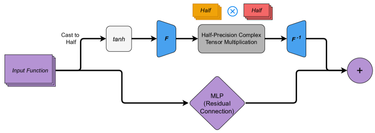
Figure 1: Overview of the half-precision FNO block. We cast the input tensor to half precision and then use a tanh pre-activation for numerical stability. We use cuFFT to run the FFT, and we compute the tensor contraction in half precision by casting each complex number to a vector.

In this work, we devise a new mixed-precision training routine for FNO which significantly improves runtime and memory usage. We start by profiling the runtime of FNO in full and mixed precision, showing the potential speedups in mixed precision. However, directly running FNO in mixed precision leads to overflow and underflow errors caused by numerical instability, typically manifesting in the first few epochs. To address this issue, we study mixed-precision stabilizing techniques, such as using a pre-activation function before the Fourier transform. We also study the loss caused by aliasing, and we show it can be mitigated by truncating the frequency modes. Based on our study, we devise a new FNO training routine, which includes a tanh pre-activation and frequency mode truncation. See Figure 1 for our full method. In order to achieve the top accuracy, we also propose a precision schedule training routine, which converts the FNO block from half, to mixed, to full precision throughout training. We conduct a thorough evaluation of our mixed precision training routines using the Navier-Stokes and Darcy flow equations, resulting in up to a 58% improvement in training throughput and a 50% reduction in GPU memory usage with little or no reduction in accuracy. We release our codebase and all materials needed to reproduce our results in the main neural operator codebase, https://github.com/neuraloperator/neuraloperator.

Our contributions. We summarize our main contributions below:

• We profile memory and runtime for FNO with full and mixed-precision training, and we conduct a study on the numerical stability of mixed-precision training of FNO, finding that tanh pre-activation is particularly suited to mitigate numerical instability.

• We show that our final mixed-precision training routine substantially decreases memory usage (up to 50%), with little or no reduction in accuracy, on the Navier-Stokes and Darcy flow equations. Our method, when combined with the recent tensorized FNO [14], achieves far better performance while also being significantly faster than the original FNO.

2 Background and Related Work

Fourier Neural Operator.

Many real-world scientific and engineering problems are based on solving partial differential equations (PDEs). Recently, many works have focused on machine learning-based methods to solve PDEs [9, 2, 24, 1]. However, the majority of these methods are based on standard neural networks and are therefore limited to a fixed input and/or output grid, although it is desirable in many applications to have a map between function spaces.

Neural operators are a new technique that addresses this limitation by directly learning maps between function spaces [22, 18, 20, 16]. The input functions to neural operators can be in any resolution or mesh, and the output function can be evaluated at any point in the domain; therefore, neural operators are discretization invariant. The Fourier neural operator (FNO) [21], inspired by the spectral method, is a highly successful neural operator [33, 7, 19, 31, 34].

Now we give a formal description of FNO. Let $\mathcal{A}:\{a:D_{\mathcal{A}}\rightarrow\mathbb{R}^{d_{\mathcal{A}}}\}$ and $\mathcal{U}:\{u:D_{\mathcal{U}}\rightarrow\mathbb{R}^{d_{\mathcal{U}}}\}$ denote the input and output function spaces, respectively. In this work, we consider the case where $D_{\mathcal{A}}=D_{\mathcal{U}}\subset\mathbb{R}^{d}$ for $d\in\mathbb{N}$. Given a dataset of pairs of initial conditions and solution functions $\{a_{j},u_{j}\}_{j=1}^{N}$, which are consistent with an operator $\mathcal{G}(a_{j})=u_{j}$ for all $1\leq j\leq N$, the goal is to learn a neural operator $\mathcal{G}_{\theta}$ that approximates $\mathcal{G}$. The primary operation in FNO is the Fourier convolution operator, $(\mathcal{K}v_{t})(x)=\mathcal{F}^{-1}(R\cdot T_{K}(\mathcal{F}v_{t}))(x),$ $\forall x\in D$, where $\mathcal{F}$ and $\mathcal{F}^{-1}$ denote the Fourier transform and its inverse, $R$ denotes a learnable transformation, $T_{K}$ denotes a truncation operation, and $v_{t}$ denotes the function at the current layer of the neural operator. In order to implement this operator on discrete data, we use the discrete Fast Fourier Transform (FFT) and its inverse (iFFT). Recent work [14] made a number of improvements to the FNO architecture, including Canonical-Polyadic factorization [13] of the weight tensors in Fourier space, which significantly improves performance while decreasing memory usage.

Mixed-Precision Training.

Mixed-precision training of neural networks consists of reducing runtime and memory usage by representing input tensors and weights (and performing operations) at lower-than-standard precision. For example, PyTorch [29] has a built-in mixed precision mode called automatic mixed precision (AMP), which places all operations at float16 rather than float32, with the exception of reduction operations, weight updates, normalization operations, and specialized operations such as ones that are complex-valued.

Mixed-precision training has been well studied for standard neural nets [35, 5, 25, 12], but has not been studied for FNO. The most similar work to ours is FourCastNet [30], a large-scale climate model that uses mixed precision with Adaptive Fourier Neural Operators [8]. However, mixed precision is not applied to the FFT or complex-valued multiplication operations, which is a key challenge that the current work addresses. Very recently, another work [6] studies method of quantization for FNO at inference time. On the other hand, our work studies quantized training and inference. Furthermore, while their metric is the number of multiplicative and addition operations, we report memory usage, wall-clock time, and throughput.

3 Mixed-Precision FNO

In this section, we first discuss the potential speedups when using mixed-precision FNO, then we address the issue of numerical stability for mixed-precision FNO, and finally, we devise and run our final training pipeline.

Throughout this section, we run experiments on two datasets. The first dataset is the two-dimensional Navier-Stokes equation for a viscous, incompressible fluid on the unit torus.

$$\partial_{t}\omega+\nabla^{\bot}\phi\cdot\omega=\frac{1}{\text{Re}}\Delta\omega+f,\quad \text{for }x\in\mathbb{T}^{2},~{}t\in(0,T]$$

$$-\Delta\phi=\omega,\quad\int_{\mathbb{T}^{2}}\phi=0,\quad \text{for }x\in\mathbb{T}^{2},~{}t\in(0,T]$$ (1)

$$\omega(0,\cdot)=0~{}\quad$$

where $\mathbb{T}^{2}\cong[0,2\pi)^{2}$ is the unit torus, $f\in L^{2}(\mathbb{T}^{2},\mathbb{R})$ is a forcing function, and $\text{Re}>0$ is the Reynolds number. The goal is to predict $\omega(5,\cdot)$, that is, the weak solution to Equation 1 at 5 timesteps into the future. We use the dataset from prior work [14], which sets $\text{Re}=500$ and generates forcing functions from the Gaussian measure, $\mathcal{N}(0,27(-\Delta+9I)^{-4})$, and computes the solution function via a pseudo-spectral solver [3]. There are 10 000 training and 2 000 test samples.

The second dataset is the steady-state two-dimensional Darcy flow equation, which is a second-order, linear, elliptic PDE.

$$-\nabla\cdot(a(x)\nabla u(x))=f(x),\quad \text{for }x\in D$$ (2)

$$u(x)=0,\quad \text{for }x\in\partial D$$ (3)

where $D=(0,1)^{2}$ is the unit square. We fix $f\equiv 1$ and seek to learn the operator $\mathcal{G}^{\dagger}:a\mapsto u$, the mapping from the diffusion coefficient to the solution function. There are 5 000 training and 1 000 test samples. The resolution for both datasets is $128\times 128$.

3.1 Potential Speedup of Mixed-Precision FNO

We compare the runtime of FNO in full and mixed precision. First, we run mixed precision via Automatic Mixed Precision (AMP) [29]. It places all operations into half precision (from float32 to float16) with a few exceptions: reduction operations, such as computing the sum or mean of a tensor; weight updates; normalization layers; and operations involving complex numbers. The first three exceptions are due to the additional precision needed for operations that involve small numbers or small differences among numbers; the last one is due to the lack of support for half-precision complex datatype in PyTorch [29]. Therefore, we devise a custom half-precision implementation of the FNO block for complex-valued operations.

First, we use the cuFFT library [27] to run both the FFT and iFFT operations in half precision. Next, in order to run the tensor multiplication in half precision, we simply cast the complex-valued input tensor into a real-valued tensor with an extra dimension, for the real part and imaginary part. For the case of tensorized FNO [14], we achieve additional speedups using tensorly [15] by computing the optimal einsum path at the start of training and caching it.

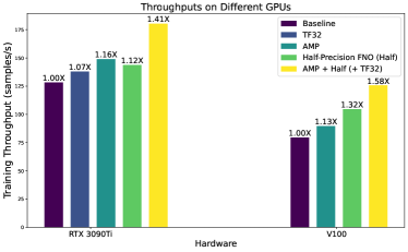
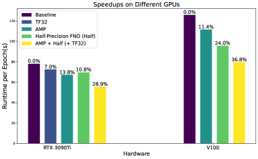
Figure 2: Training throughput and runtime as a function of the method, on different hardware. For mixed-precision FNO + AMP, we consistently observe an improvement of throughput up to 1.58X over the baseline, and a speedup of up to 36.8%. Our method also improves upon using only AMP in throughput by over 1.3X. Batch sizes are selected to fully utilize each GPU, and specific numbers can be found in the appendix.

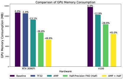
Figure 3: Reduction in GPU memory consumption on different hardware. Under the same setting, our method reduces FNO’s GPU memory footprint by close to 50%, with Half-Precision FNO contributing the most reduction.

Based on the maximum training throughput on the Navier Stokes dataset described above, we show that our mixed-precision approach increases throughput to 1.41X on Ampere GPUs (RTX 3090Ti) and to 1.58X on Volta GPUs (V100), while improving upon the AMP baseline by up to 1.3X. For a fixed batch size on V100, we measure the training time per epoch and find that AMP and half-precision-Fourier operations result in 11.4% and 24.0% speedups, respectively, and together result in a 36.8% speedup; see Figure 2. For GPU memory usage, we observe a significant reduction of up to 50% for the same fixed batch size. Our half-precision implementation of FNO is responsible for most of the reduction, as the FNO layers remain the main GPU memory bottleneck; see Figure 3 We also find that the memory reduction for AMP+half-precision-Fourier on the Darcy flow dataset is 24.4% on RTX 3090Ti. However, for both datasets, running in mixed precision results in numerical instability, especially for the forward and inverse FFTs. In particular, the forward FFT causes overflow in first few epochs of training. In the next section, we consider stabilizing techniques for these operations.

3.2 Stabilizing Mixed-Precision FFT

Mixed-precision training is prone to underflow and overflow because the dynamic range of half precision is significantly smaller than full precision. We empirically show that naïve methods such as scaling, normalization, and alternating half and full precision do not fix the numerical instability. In particular, a simple idea is to scale down all values by adding a fixed pointwise division operation before the FFT. However, this does not work: due to the presence of outliers, all values must be scaled down by significant amount (a factor of at least $10^{4}$). This forces all numbers into a very small range, which half precision cannot distinguish, preventing the model from converging to an acceptable performance. We also find that changing the normalization of the Fourier transform (essentially equivalent to scaling) does not fix the numerical instability.

Table 1: Comparison of different pre-activation functions used for numerical stability. tanh achieves the fastest runtime without significantly compromising on loss. Since our focus now is on numerical stability, we compare only the average train loss over the 5 final epochs (we compare the test losses in Section 3.3).

Fourier	AMP	Pre-	Runtime	Train
Precision	(T/F)	Activation	per epoch	loss
Full	F	N/A	44.4	0.0457
Full	T	N/A	42.3	0.0457
Half	F	N/A	N/A	N/A
Half	T	hard-clip	37.1	0.0483
Half	T	2$\sigma$-clip	40.0	0.0474
Half	T	tanh	36.5	0.0481

We also find normalization simply scales by the variance of the batch or layer, which faces the same problems as above. And due to the stochastic yet consistent nature of the overflow errors, alternating between half and full precision also does not mitigate overflow.

On the other hand, we show that pre-activation is a very effective method for overcoming numerical instability. Pre-activation is the practice of adding a nonlinearity before a typical ‘main’ operation such as a convolution [10]. Unlike scaling and normalization, pre-activations such as tanh force all values within the range $[-1,1]$ while being robust to outliers: the shape of tanh maintains the trends in the values near the mean.

We observe that only adding a pre-activation before the first FFT still results in overflow in the next FFT. Therefore, we add a pre-activation function before every forward FFT in the architecture. We test AMP+half-precision-Fourier with three pre-activation functions: tanh (the hyperbolic tangent function), hard-clip (the identity function, but mapping all values $\geq 1$ to 1 and $\leq-1$ to -1), and 2$\sigma$-clip (similar to hard clip, but using 2 times the standard deviation as threshold values). For this ablation study, we train each model for 100 epochs using the default hyperparameters from the FNO architecture [21, 14]; see Table 1. We find that tanh is the most promising pre-activation overall: it is the fastest, it is smooth and fully-differentiable, and since the operation is pointwise, tanh maintains discretization invariance of the FNO architecture. Therefore, we use tanh in our final experiments later in this section.

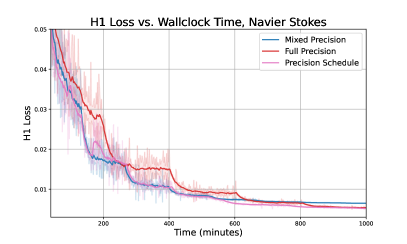
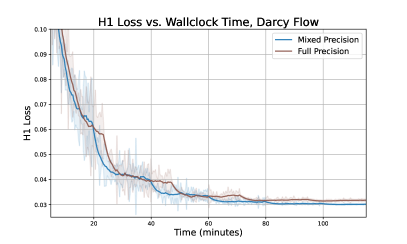
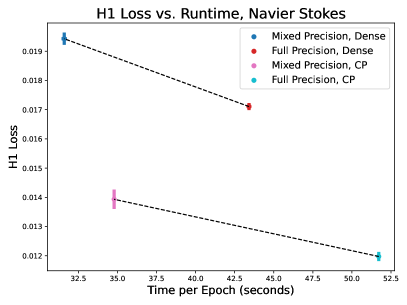
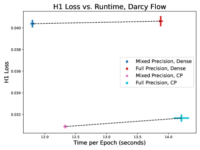
Figure 4: Test H1 error curves for FNO on the Navier Stokes (top left) and Darcy flow (top right) datasets. Pareto frontier for FNO on the Navier Stokes (bottom left) and Darcy flow (bottom right) datasets, for Canonical-Polyadic factorization (CP) or no factorization (Dense). We train each model for 500 epochs, and we plot the standard deviation across 3 trials for each setting.

3.3 Final Training Pipeline

Based on the results from the previous sections, we compare full-precision FNO to mixed-precision FNO with tanh pre-activation, on the full training pipeline consisting of 500 epochs. As in prior work [19, 14], training is done using the H1 Sobolev norm [4, 19]. We perform evaluation with the $H^{1}$ norm, and we also present results with the $L^{2}$ norm in Appendix A. We run experiments on both Navier Stokes and Darcy flow data, with and without Canonical-Polyadic factorization [13] of the weight matrices (which was recently shown to substantially improve performance and memory usage of FNO [14]).

In addition to running full precision and AMP+HALF+TANH, we also test a precision schedule, in which the first 25% of training is in AMP+HALF+TANH, the middle 50% of training puts the FFT in full precision, and the final 25% of training is in full precision. See Figure 4 (left) for results on the Navier Stokes dataset. Across all settings, naïvely running mixed-precision results in NaN’s after a few epochs, but adding tanh pre-activation allows the model to converge much faster and with nearly the same final performance. AMP+HALF+TANH achieves a 34% reduction in runtime per epoch on an NVIDIA Tesla V100 GPU. While AMP+HALF+TANH converges to an error that is 6-11% worse than full-precision, the precision schedule converges to an error that is 10% better than full precision, due to its better anytime performance.

We also test our method on the Darcy flow dataset described in Section 3. Similar to the Navier Stokes dataset, we find that simply running the FFT in half precision leads to numerical instability, but running AMP+HALF+TANH gives an 18% reduction in runtime with no increase in loss. See Figure 4 (right). This confirms that our findings from Section 3.2 can generalize to other datasets.

tanh Ablation Study.

Since our full method, AMP+HALF+TANH uses a hyperbolic tangent preactivation, a natural question is to ask how a hyperbolic tangent would affect the full precision FNO model with no other changes. In Table 2, we answer this question by running the full precision FNO model on the Navier Stokes dataset. We find that there is no noticeable change in the test losses, and the runtime-per-epoch increases by 0.8 seconds, or 1.6%. This concludes that tanh is a reasonable and practical choice to improve numerical stability for half precision methods.

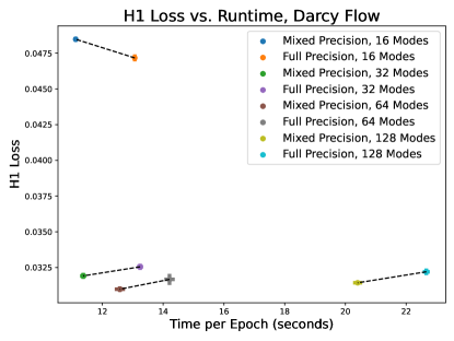
Figure 5: Comparison of the full-precision and mixed-precision (AMP+HALF+TANH) FNO with different frequency modes, on the Darcy flow dataset. For 16 frequency modes, the half precision error (compared to full precision) is higher than for 32, 64, or 128 modes.

Table 2: Ablation study on full-precision FNO with and without tanh on the Navier Stokes dataset. There is no noticeable change in accuracy, showing that tanh is a practical choice to improve numerical stability in low precision methods.

	$H^{1}$	$L^{2}$	time-per-epoch (sec)
Full precision	0.0121	0.00470	51.72
Full precision + tanh	0.0122	0.00465	52.56

Frequency Mode Ablation Study.

Recall that in the FNO architecture, after the FFT, we crucially truncate to a fixed number of frequency modes to improve performance, typically $\nicefrac{{1}}{{3}}$ to $\nicefrac{{2}}{{3}}$. Now we run an ablation study on the number of frequency modes used in the FNO architecture. We run frequency modes $\{16,32,64,128\}$ on the $128\times 128$ Darcy flow dataset in full and half precision; see Figure 5. We find that using two few frequency modes hurts accuracy substantially, while using too many frequency modes increases runtime substantially. There is not a significant difference between half precision and full precision, for all frequencies.

Next, we run an experiment on synthetic data to demonstrate that the error caused by half precision is higher for higher frequencies, relative to the amplitude. We create a signal based on sine and cosine waves with frequencies from 1 to 10, with randomly drawn, exponentially decaying amplitudes. Then we plot the Fourier spectrum in full and half precision, as well as the absolute error of the half-precision spectrum as a percentage of the true amplitudes. See Figure 6; we find that the percentage error exponentially increases. Since in real-world data, the energy is concentrated in the lowest frequency modes, and the higher frequency modes are truncated, this gives further justification for our half precision method.

Resolution Invariance.

An important property of neural operators is their resolution invariance, meaning that they can be trained on one resolution and tested on a higher resolution (zero-shot super resolution). In order to show that our low-precision training pipeline maintains resolution invariance, we show zero-shot super resolution results. We use the Navier Stokes dataset, trained on $128\times 128$ resolution (the same setting and model as Figure 4), and tested on $256\times 256$, $512\times 512$, and $1024\times 1024$ resolutions; see Table 3. We find that similarly to $128\times 128$ test data, half-precision has a small decrease in accuracy compared to full precision, and using a precision schedule achieves significantly better performance with the same training time.

4 Conclusions and Future Work

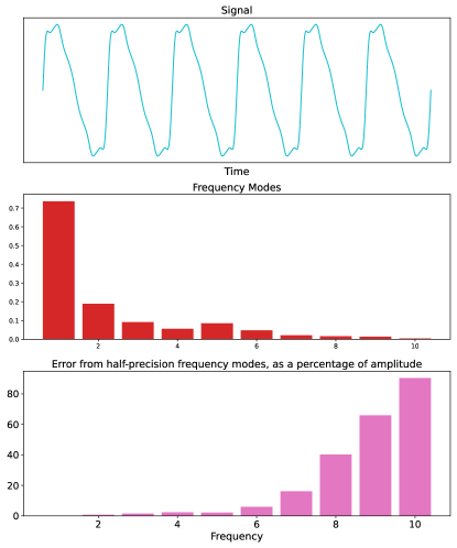
Figure 6: Synthetic signal (top), its frequency modes (middle), and the error due to half precision, as a percentage of the amplitude (bottom). The percentage error increases for higher frequencies.

In this work, we studied the numerical stability of half-precision training for FNO, and we devised a new training routine which results in a significant improvement in runtime and memory usage. Specifically, we showed that using tanh pre-activation before the Fourier transform mitigates numerical instability. We also showed that the range of half precision is too small to learn high frequency modes, and therefore, reducing the learnable frequency modes also helps performance. We show that with these modifications, running FNO in half precision results in up to a 50% reduction in memory, with little to no decrease in accuracy, on the Navier Stokes and Darcy flow equations. Overall, half-precision FNO makes it possible to train on significantly larger datapoints with the same batch size. Going forward, we plan to apply this on real-world applications that require super resolution to enable larger scale training.

Table 3: Zero-shot super resolution. FNO is resolution invariant. We test zero-shot super-resolution by training each model on $128\times 128$ resolution for 19 hours. We find that half-precision has a small decrease in accuracy compared to full precision, and using a precision schedule achieves significantly better accuracy with the same training time.

	128x128		256x256		512x512		1024x1024
	$H^{1}$	$L^{2}$	$H^{1}$	$L^{2}$	$H^{1}$	$L^{2}$	$H^{1}$	$L^{2}$
Full precision	0.00557	0.00213	0.00597	0.00213	0.00610	0.00213	0.00616	0.00213
Half precision	0.00624	0.00236	0.00672	0.00228	0.00688	0.00226	0.00693	0.00226
Precision schedule	0.00503	0.00170	0.00542	0.00170	0.00555	0.00170	0.00558	0.00170

Broader Societal Impact

We do not foresee any strongly negative impacts, in terms of the broader societal impacts. In fact, this work may help to reduce the carbon footprint of scientific computing experiments.

Recently, the overall daily amount of computation used for machine learning has been increasing exponentially [32]. Relatedly, model sizes are also increasing fast [28]. Leveraging the power of mixed-precision computing for neural operators can make it possible to design better models for important tasks such as climate modeling [30] and carbon storage [34].

Appendix A Additional Details from Section 3

We present additional experiments similar to the results in Section 3, but using the $L^{2}$ metric instead of $H^{1}$. In Figure 7, we plot an ablation study on the number of frequency modes for Darcy flow, similar to Figure 5, but with $L^{2}$ loss. We see that the overall trends are similar, but test $L^{2}$ loss is noisier than test L1 loss; this makes sense, because the training loss is $H^{1}$. In Figure 8, we plot the performance-vs-time and Pareto frontier plots for Navier Stokes and Darcy flow, similar to Figure 4, but with $L^{2}$ loss. As before, we see largely the same trends as with $H^{1}$ loss, but the results are noisier. In Table 4, we plot the final performance from the models run in Figure 4.

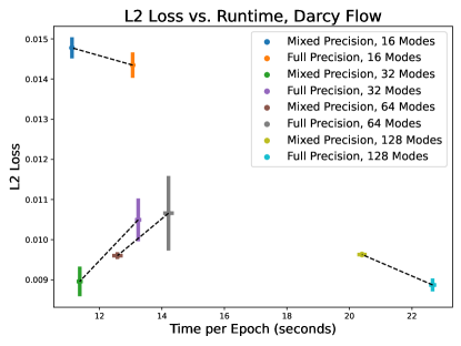
Figure 7: Comparison of the full-precision and mixed-precision (AMP+HALF+TANH) FNO with different frequency modes, on the Darcy flow dataset.

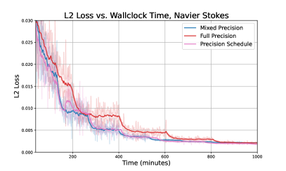
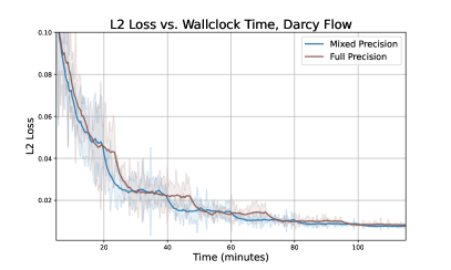
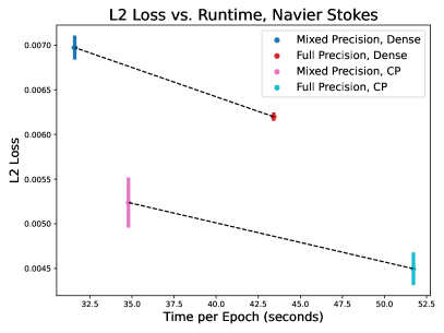
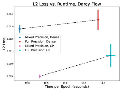
Figure 8: Test $L^{2}$ error curves for FNO on the Navier Stokes (top left) and Darcy flow (top right) datasets. Pareto frontier for FNO on the Navier Stokes (bottom left) and Darcy flow (bottom right) datasets, for Canonical-Polyadic factorization (CP) or no factorization (Dense). We train each model for 500 epochs, and we plot the standard deviation across 3 trials for each setting.

Table 4: Results for FNO with full precision, half precision, and precision schedule. All results are the average over 3 seeds trained to 19 hours each (which is the time it takes full precision FNO to reach 500 epochs).

	$H^{1}$	$L^{2}$	time-per-epoch (sec)
Full precision	$.00536\pm 2.1e-5$	$.00214\pm 3.5e-5$	121.4
Half precision	$.00645\pm 6.6e-5$	$.00212\pm 1.4e-5$	80.2
Precision schedule	$.00515\pm 8.3e-5$	$.00812\pm 4.1e-5$	80.2, 83.8, 121.4

References

- [1] Jonas Adler and Ozan Öktem. Solving ill-posed inverse problems using iterative deep neural networks. Inverse Problems, 33(12):124007, 2017.
- [2] Saakaar Bhatnagar, Yaser Afshar, Shaowu Pan, Karthik Duraisamy, and Shailendra Kaushik. Prediction of aerodynamic flow fields using convolutional neural networks. Computational Mechanics, 64:525–545, 2019.
- [3] Gary J Chandler and Rich R Kerswell. Invariant recurrent solutions embedded in a turbulent two-dimensional kolmogorov flow. Journal of Fluid Mechanics, 722:554–595, 2013.
- [4] Wojciech M Czarnecki, Simon Osindero, Max Jaderberg, Grzegorz Swirszcz, and Razvan Pascanu. Sobolev training for neural networks. Proceedings of the Annual Conference on Neural Information Processing Systems (NeurIPS), 30, 2017.
- [5] Christopher De Sa, Megan Leszczynski, Jian Zhang, Alana Marzoev, Christopher R Aberger, Kunle Olukotun, and Christopher Ré. High-accuracy low-precision training. arXiv preprint arXiv:1803.03383, 2018.
- [6] Winfried van den Dool, Tijmen Blankevoort, Max Welling, and Yuki M Asano. Efficient neural pde-solvers using quantization aware training. arXiv preprint arXiv:2308.07350, 2023.
- [7] Vignesh Gopakumar, Stanislas Pamela, Lorenzo Zanisi, Zongyi Li, Anima Anandkumar, and MAST Team. Fourier neural operator for plasma modelling. arXiv preprint arXiv:2302.06542, 2023.
- [8] John Guibas, Morteza Mardani, Zongyi Li, Andrew Tao, Anima Anandkumar, and Bryan Catanzaro. Adaptive fourier neural operators: Efficient token mixers for transformers. In Proceedings of the International Conference on Learning Representations (ICLR), 2021.
- [9] Gaurav Gupta, Xiongye Xiao, and Paul Bogdan. Multiwavelet-based operator learning for differential equations. Proceedings of the Annual Conference on Neural Information Processing Systems (NeurIPS), 34:24048–24062, 2021.
- [10] Kaiming He, Xiangyu Zhang, Shaoqing Ren, and Jian Sun. Identity mappings in deep residual networks. In European Conference on Computer Vision, pages 630–645. Springer, 2016.
- [11] Hrvoje Jasak. Openfoam: open source cfd in research and industry. International Journal of Naval Architecture and Ocean Engineering, 1(2):89–94, 2009.
- [12] Xianyan Jia, Shutao Song, Wei He, Yangzihao Wang, Haidong Rong, Feihu Zhou, Liqiang Xie, Zhenyu Guo, Yuanzhou Yang, Liwei Yu, et al. Highly scalable deep learning training system with mixed-precision: Training imagenet in four minutes. arXiv preprint arXiv:1807.11205, 2018.
- [13] Tamara G Kolda and Brett W Bader. Tensor decompositions and applications. SIAM review, 51(3):455–500, 2009.
- [14] Jean Kossaifi, Nikola Borislavov Kovachki, Kamyar Azizzadenesheli, and Anima Anandkumar. Multi-grid tensorized fourier neural operator for high resolution PDEs, 2023.
- [15] Jean Kossaifi, Yannis Panagakis, Anima Anandkumar, and Maja Pantic. Tensorly: tensor learning in python. The Journal of Machine Learning Research, 20(1):925–930, 2019.
- [16] Nikola Kovachki, Zongyi Li, Burigede Liu, Kamyar Azizzadenesheli, Kaushik Bhattacharya, Andrew Stuart, and Anima Anandkumar. Neural operator: Learning maps between function spaces with applications to pdes. Journal of Machine Learning Research, 24(89):1–97, 2023.
- [17] Remi Lam, Alvaro Sanchez-Gonzalez, Matthew Willson, Peter Wirnsberger, Meire Fortunato, Alexander Pritzel, Suman Ravuri, Timo Ewalds, Ferran Alet, Zach Eaton-Rosen, et al. Graphcast: Learning skillful medium-range global weather forecasting. arXiv preprint arXiv:2212.12794, 2022.
- [18] Zongyi Li, Nikola Kovachki, Kamyar Azizzadenesheli, Burigede Liu, Kaushik Bhattacharya, Andrew Stuart, and Anima Anandkumar. Neural operator: Graph kernel network for partial differential equations. arXiv preprint arXiv:2003.03485, 2020.
- [19] Zongyi Li, Nikola Kovachki, Kamyar Azizzadenesheli, Burigede Liu, Kaushik Bhattacharya, Andrew Stuart, and Anima Anandkumar. Learning dissipative dynamics in chaotic systems. arXiv preprint arXiv:2106.06898, 2021.
- [20] Zongyi Li, Nikola Kovachki, Kamyar Azizzadenesheli, Burigede Liu, Andrew Stuart, Kaushik Bhattacharya, and Anima Anandkumar. Multipole graph neural operator for parametric partial differential equations. Proceedings of the Annual Conference on Neural Information Processing Systems (NeurIPS), 33:6755–6766, 2020.
- [21] Zongyi Li, Nikola Borislavov Kovachki, Kamyar Azizzadenesheli, Kaushik Bhattacharya, Andrew Stuart, Anima Anandkumar, et al. Fourier neural operator for parametric partial differential equations. In Proceedings of the International Conference on Learning Representations (ICLR), 2021.
- [22] Zongyi Li, Hongkai Zheng, Nikola Kovachki, David Jin, Haoxuan Chen, Burigede Liu, Kamyar Azizzadenesheli, and Anima Anandkumar. Physics-informed neural operator for learning partial differential equations. arXiv preprint arXiv:2111.03794, 2021.
- [23] Burigede Liu, Nikola Kovachki, Zongyi Li, Kamyar Azizzadenesheli, Anima Anandkumar, Andrew M Stuart, and Kaushik Bhattacharya. A learning-based multiscale method and its application to inelastic impact problems. Journal of the Mechanics and Physics of Solids, 158:104668, 2022.
- [24] Lu Lu, Pengzhan Jin, and George Em Karniadakis. Deeponet: Learning nonlinear operators for identifying differential equations based on the universal approximation theorem of operators. arXiv preprint arXiv:1910.03193, 2019.
- [25] Paulius Micikevicius, Sharan Narang, Jonah Alben, Gregory Diamos, Erich Elsen, David Garcia, Boris Ginsburg, Michael Houston, Oleksii Kuchaiev, Ganesh Venkatesh, et al. Mixed precision training. arXiv preprint arXiv:1710.03740, 2017.
- [26] Tung Nguyen, Johannes Brandstetter, Ashish Kapoor, Jayesh K Gupta, and Aditya Grover. Climax: A foundation model for weather and climate. arXiv preprint arXiv:2301.10343, 2023.
- [27] NVIDIA. cufft official documentation, release 12.2, 2023.
- [28] OpenAI. Ai and compute. https://openai.com/blog/ai-and-compute/, 2018.
- [29] Adam Paszke, Sam Gross, Francisco Massa, Adam Lerer, James Bradbury, Gregory Chanan, Trevor Killeen, Zeming Lin, Natalia Gimelshein, Luca Antiga, et al. Pytorch: An imperative style, high-performance deep learning library. In Proceedings of the Annual Conference on Neural Information Processing Systems (NeurIPS), 2019.
- [30] Jaideep Pathak, Shashank Subramanian, Peter Harrington, Sanjeev Raja, Ashesh Chattopadhyay, Morteza Mardani, Thorsten Kurth, David Hall, Zongyi Li, Kamyar Azizzadenesheli, et al. Fourcastnet: A global data-driven high-resolution weather model using adaptive fourier neural operators. arXiv preprint arXiv:2202.11214, 2022.
- [31] Peter I Renn, Cong Wang, Sahin Lale, Zongyi Li, Anima Anandkumar, and Morteza Gharib. Forecasting subcritical cylinder wakes with fourier neural operators. arXiv preprint arXiv:2301.08290, 2023.
- [32] Roy Schwartz, Jesse Dodge, Noah A Smith, and Oren Etzioni. Green ai. Communications of the ACM, 63(12):54–63, 2020.
- [33] Gege Wen, Zongyi Li, Kamyar Azizzadenesheli, Anima Anandkumar, and Sally M Benson. U-fno—an enhanced fourier neural operator-based deep-learning model for multiphase flow. Advances in Water Resources, 163:104180, 2022.
- [34] Gege Wen, Zongyi Li, Qirui Long, Kamyar Azizzadenesheli, Anima Anandkumar, and Sally M Benson. Accelerating carbon capture and storage modeling using fourier neural operators. arXiv preprint arXiv:2210.17051, 2022.
- [35] Jiawei Zhao, Steve Dai, Rangharajan Venkatesan, Brian Zimmer, Mustafa Ali, Ming-Yu Liu, Brucek Khailany, William J Dally, and Anima Anandkumar. Lns-madam: Low-precision training in logarithmic number system using multiplicative weight update. IEEE Transactions on Computers, 71(12):3179–3190, 2022.