Identifying regime switches through Bayesian wavelet estimation: evidence from flood detection in the Taquari River Valley

Abstract

Two-component mixture models have proved to be a powerful tool for modeling heterogeneity in several cluster analysis contexts. However, most methods based on these models assume a constant behavior for the mixture weights, which can be restrictive and unsuitable for some applications. In this paper, we relax this assumption and allow the mixture weights to vary according to the index (e.g., time) to make the model more adaptive to a broader range of data sets. We propose an efficient MCMC algorithm to jointly estimate both component parameters and dynamic weights from their posterior samples. We evaluate the method’s performance by running Monte Carlo simulation studies under different scenarios for the dynamic weights. In addition, we apply the algorithm to a time series that records the level reached by a river in southern Brazil. The Taquari River is a water body whose frequent flood inundations have caused various damage to riverside communities. Implementing a dynamic mixture model allows us to properly describe the flood regimes for the areas most affected by these phenomena.

1 Introduction

In several data analysis problems, we want to cluster observations between two groups. For instance, in many clinical studies, the goal is to classify patients according to disease absent or present (see Hall and Zhou,, 2003, Rindskopf and Rindskopf,, 1986, Hui and Zhou,, 1998). In contamination problems found in astronomy investigations, on the other hand, the aim is to separate the objects of interest, called members (e.g., stars), from foreground/background objects contaminating the sample, known as contaminants (see Walker et al.,, 2009). In genetics, studies based on microarray data are usually driven to detecting differentially expressed genes under two conditions, e.g., “healthy tissue versus diseased tissue” (see Bordes et al.,, 2006).

To address these scenarios of bimodal data sets, two-component mixture models have shown to be excellent alternatives to cluster data observations within the group that better describes their features (Patra and Sen,, 2016). In this context, the mixture model with two components will assume that the sample of data observations $y_{1},\dots,y_{n}$ is, in fact, the realization of a random variable $Y$ that belongs to a population composed of two subpopulations, known as mixture components. Thus, at each point $t$, $t=1,\dots,n$, $Y$ is fitted according to some of the mixture components, dictated by a mixture weight $\alpha$.

This setting may be very restrictive to some data sets. For instance, in epidemiological studies that evaluate the response to medications, the probability of classifying a patient in the group of “disease present” must be allowed to vary across time so that the longitudinal effect of the treatment can be properly measured. The same issue arises in quality control problems, where the probability of the supervised system operating in a failure-free regime is also not constant over time. In order to classify those features properly, under a mixture model assumption, the mixture weight should be allowed to vary according to the index (which could be time or location). In other words, it would be appropriate for the mixture weight to present a dynamic behavior.

Assuming dynamic mixture weights for mixture models is an extension that has already been applied in different areas, from traffic flow applications (see Nagy et al.,, 2011) to investigations in genetics (see Montoril et al.,, 2019; 2021). As discussed in Montoril et al., (2021), this generalization is similar to the extension of Hidden Markov Models (HMM) into non-homogeneous Hidden Markov Models (NHMM), first described by Hughes and Guttorp, (1994). In both scenarios, one generalizes the model by considering unobserved varying probabilities. In the case of mixture models, those dynamic probabilities are the mixture weights, whereas, in HMM, they are the transition probabilities. It is important to emphasize that, although connected, dynamic mixture weights and transition probabilities are different things.

Considering a “non-homogeneous” structure for the mixture model implies that, besides estimating the dynamic mixture weights, one also needs to estimate the component parameters, and that increases the challenge. For instance, in Montoril et al., (2019), from a frequentist approach, the authors rely on wavelets to perform the estimation of the dynamic weights, where they transform the data in order to deal with a nonparametric heteroscedastic regression. Nonetheless, their procedure depends on assuming known means and variances for the mixture components, which, in practice, may be unrealistic.

In this work, unlike the aforementioned paper, the leading motivation is to provide a Bayesian approach that estimates not only the dynamic mixture weights but also the component parameters of a two-component mixture model. To accomplish this goal, we propose an efficient Gibbs sampling algorithm, which allows the distribution of the posterior draws to be used for inference purposes. Regarding the dynamic mixture weights, we use the data augmentation method by Albert and Chib, (1993) and incorporate Bayesian wavelet denoising techniques to estimate the dynamic behavior of the mixture weight. We do this to exploit the good properties of wavelets in curves’ estimation.

Wavelets are families of basis functions that can be used to represent other functions, signals, and images as a series of successive approximations (Härdle et al.,, 2012, Abramovich et al.,, 2000). In statistical applications, these mathematical tools have been successfully used to solve problems in nonparametric regression (see Donoho and Johnstone,, 1994, Cai and Brown,, 1999); density estimation (see Donoho, 1993a, , Donoho et al.,, 1996, Hall and Patil,, 1995); time series analysis (see, e.g., Morettin,, 1996, Priestley,, 1996, Percival and Walden,, 1999); among many other areas. There is a vast literature that provides a review of wavelets in statistics (see, e.g., Vidakovic,, 1999, Ogden,, 1997).

In this paper, wavelet bases are applied to enable the estimation of the dynamic mixture weights. To review the mathematical background and the terminology associated with the wavelet theory, in the following section, we provide a short introduction to the wavelet basis functions; the discrete wavelet transform (DWT); and, the Bayesian approach for denoising in a wavelet-based scenario. The remainder of the paper is organized as follows. In Section 3, we describe the dynamic mixture model considered in this paper and give details related to the MCMC sampling scheme constructed to perform the estimation. In Section 4, we present some numerical experiments. We first conduct Monte Carlo simulations to evaluate the method in a controlled setting. Then, we apply the MCMC algorithm to a river data set to identify periods when flood inundations occurred.

2 Wavelets

In this work, we use the term wavelets to refer to a system of orthonormal basis functions for $L_{2}([0,1])$ or $L_{2}(\mathbb{R})$. The bases are generated by dyadic translations and dilations of the functions $\varphi(\cdot)$ and $\psi(\cdot)$, known, respectively, as the scaling and wavelet functions. These systems of integer-translates and dilates are given by

$$\varphi_{j_{0}k}(t) =2^{j_{0}/2}\varphi(2^{j_{0}}t-k),\quad k\in\mathbb{Z},$$

$$\psi_{jk}(t) =2^{j/2}\psi(2^{j}t-k),\quad j,k\in\mathbb{Z}.$$

Thus, for any integer $j_{0}$ and $J$, a periodic function $f(t)\in L_{2}([0,1])$ can be approximated in $L_{2}$-sense as the projection onto a multiresolution space $V_{J}$:

$$f(t)=\sum\limits_{k=0}^{2^{j_{0}}-1}c_{j_{0}k}\varphi_{j_{0}k}(t)+\sum\limits_{j=j_{0}}^{J-1}\sum\limits_{k=0}^{2^{j}-1}d_{jk}\psi_{jk}(t),$$

where $c_{j_{0}k}$’s are known as scaling coefficients and $d_{jk}$’s are called detail coefficients. The former are associated with the coarsest resolution level in witch $f(t)$ was decomposed, $j_{0}$. As a result, they capture the gross structure of $f(t)$. The detail coefficients, on the other hand, being linked to finer resolution levels, can capture local information about $f(t)$. Put simply, in moving from a coarser resolution level $j$ to a finer $j+1$, we are increasing the resolution at which a function is approximated, thus the expansion coefficients become more descriptive about the local features of $f(t)$.

In practice, we access $f(t)\in L_{2}([0,1])$ through a grid of points in time or space in which $f$ is applied. Therefore, consider $\bm{f}=(f(1/n),f(2/n),\dots,f(n/n))^{T}$ to be a vector of samples of $f(t)$ on an equispaced grid of $n$ points, with $n=2^{J}$, for some positive integer $J$. To obtain the scaling and detail coefficients that approximate $\bm{f}$, we perform the discrete wavelet transform (DWT) of $\bm{f}$. In matrix notation, the DWT of $\bm{f}$ is

$$\bm{\theta}=\bm{Wf},$$ (1)

where $\bm{\theta}=(c_{00},d_{00},\bm{d}_{1}^{T},\dots,\bm{d}_{J-1}^{T})^{T}$ is a vector of size $n$, having both scaling and detail coefficients $\bm{d}_{j}=(d_{j0},d_{j1},\dots,d_{j2^{j}-1})^{T}$, and $\bm{W}$ is the DWT matrix with $(jk,i)$ entry given by $W_{jk,i}\sqrt{n}\approx\psi_{jk}(i/n)=2^{j/2}\psi(2^{j}i/n-k)$, $k=0,\dots,2^{j}-1$, $j=1,\dots,J-1$. (Abramovich et al.,, 1998). By orthogonality, the multiplication $\bm{W^{T}\theta}$ recovers the signal $\bm{f}$. This transformation from wavelet coefficients to fitted values is known as the inverse discrete wavelet transform (IDWT).

One of the main advantages provided by the DWT is the sparse representation generally achieved. As shown by Donoho, 1993b , wavelets are unconditional bases for a range of function spaces, such as Hölder and Sobolev spaces, as well as spaces suitable for representing functions of ‘bounded variation’. As an aside, it is also worth mentioning that using Mallat’s pyramid algorithm (Mallat,, 1989), the DWT and IDWT are performed requiring only $\mathcal{O}(n)$ operations, which makes them very efficient in terms of computational speed and storage. These properties help to explain why wavelet bases are excellent tools to address problems of data analysis. In the following section, we present a brief review of handling the denoising problem within the wavelet domain, emphasizing the Bayesian framework due to its central role in the estimation process of this paper.

2.1 Bayesian wavelet denoising

Consider the nonparametric regression model

$$\bm{y}=\bm{f}+\bm{e},$$ (2)

where $\bm{y}=(y_{1},\dots,y_{n})^{T}$ is the vector of observed values, $\bm{f}=(f(1/n),\dots,f(n/n))^{T}$ is the function of interest applied to a grid of $n$ equally spaced points, and $\bm{e}=(e_{1},\dots,e_{n})^{T}$ is a vector of zero-mean random variables. For most applications, $e_{t}$’s are independent and identically distributed normal random variables with zero mean and constant variance $\sigma^{2}$. The goal of nonparametric regression is to recover the unknown function $f$ from the noisy observations $\bm{y}$.

With that in mind, Donoho and Johnstone, (1994) propose to transform the observations $\bm{y}$ to the wavelet domain, shrink the noisy wavelet coefficients or even equal them to zero, based on some threshold rule, and then estimate $\bm{f}$ by applying the IDWT to the regularized coefficients. This method is known in the literature as wavelet shinkage. Therefore, let $n$ be a power of two, $n=2^{J}$ for some positive integer $J$. Then, we can represent (2) in the wavelet domain as

$$\bm{d}^{*}=\bm{\theta}+\bm{\varepsilon},$$ (3)

where $\bm{d}^{*}=\bm{Wy}$, $\bm{\theta}=\bm{Wf}$, and $\bm{\varepsilon}=\bm{We}$, with $\bm{W}$ being the DWT matrix.

From a Bayesian perspective, the wavelet shrinkage technique consists in assigning a prior distribution to each wavelet coefficient of the unknown function. The idea is that, by choosing a prior able to capture the sparseness associated with most wavelet decompositions, we can estimate $\bm{\theta}$, by imposing some Bayes rule on the resulting posterior distribution of the wavelet coefficients. Then, applying the IDWT to the estimated $\bm{\theta}$ gives us an estimation of $\bm{f}$.

One of the most appropriate prior choices for modeling wavelet coefficients are the spike and slab priors. First consolidated within Bayesian variable selection methods (George and McCulloch,, 1993), these kinds of prior are a mixture between two components: one that concentrates its mass at values close to zero or even in zero (Dirac delta) and another whose mass is spread over a wide range of possible values for the unknown parameters. Choosing this mixture as prior to the distribution of wavelet coefficients allows the first component, known as spike, to capture the null wavelet coefficients, while the second component, called slab, describes the coefficients associated with the unknown function.

A spike and slab prior frequently assigned to wavelet coefficients is the mixture between a point mass at zero and a Gaussian distribution (see, e.g., Abramovich et al.,, 1998). In this scenario, each detail wavelet coefficient is distributed following

$$\begin{split}&\pi_{j}\text{N}(0,\upsilon_{j}^{2})+(1-\pi_{j})\delta_{0}(\theta_{jk}),\\ \end{split}$$ (4)

$k=0,1,\dots,2^{j}-1$, $j=0,1,\dots,J-1$, with $\delta_{0}$ being a point mass at zero. The prior specification is usually completed by assigning a diffuse prior to the scaling coefficient at the coarsest level $c_{00}$. Thus, the sample scaling coefficient obtained from the DWT of the data estimates $c_{00}$ (Abramovich et al.,, 1998).

Under the prior (LABEL:eq:prior_normal), the posterior distribution for each detail coefficient is also a mixture between a Gaussian distribution and $\delta_{0}$, given by

$$\begin{split}\theta_{jk}|d_{jk}^{*}&\sim\pi_{\text{post}}\text{N}\left(\frac{\upsilon_{j}^{2}}{1+\upsilon_{j}^{2}}d_{jk}^{*},\frac{\upsilon_{j}^{2}}{1+\upsilon_{j}^{2}}\right)+(1-\pi_{\text{{post}}})\delta_{0}(\theta_{jk}),\\ \pi_{\text{post}}&=\frac{\pi_{j}g_{\upsilon_{j}^{2}}(d_{jk}^{*})}{\pi_{j}g_{\upsilon_{j}^{2}}(d_{jk}^{*})+(1-\pi_{j})\phi(d_{jk}^{*})},\\ \end{split}$$ (5)

$k=0,1,\dots,2^{j}-1$, $j=0,1,\dots,J-1$, where $\phi$ denotes the standard normal density and $g_{\upsilon_{j}^{2}}$ denotes the convolution between the slab component in (LABEL:eq:prior_normal) (in this case $\text{N}(0,\upsilon_{j}^{2})$) and $\phi$. Using $\gamma$ to denote the slab density and $\star$ to denote the convolution operator, we can write $g=\gamma\star\phi$. It should be stressed that, as shown by Abramovich et al., (1998), using the posterior medians as the pointwise estimates of $\bm{\theta}$ yields a thresholding rule. In other words, we are able to equal the estimated noisy coefficients to zero.

In the Empirical Bayes thresholding method by Johnstone and Silverman, 2005a , Johnstone and Silverman, 2005b , the authors propose replacing the Gaussian component in (LABEL:eq:prior_normal) with heavy-tailed distributions, such as the Laplace density. This replacement intends to provide larger estimates for the non-null coefficients than those obtained from Gaussian distributions. In this scenario, considering the Laplace density as the slab component, the prior for each detail wavelet coefficient can be written as

$$\begin{split}&\pi_{j}\gamma_{a}(\theta_{jk})+(1-\pi_{j})\delta_{0}(\theta_{jk}),\\ \end{split}$$ (6)

$k=0,1,\dots,2^{j}-1$, $j=0,1,\dots,J-1$, where $\gamma_{a}(x)$ denotes the Laplace density with scale parameter $a>0$, i.e.,

$$\gamma_{a}(x)=\frac{a}{2}\exp(-a|x|),\quad x\in\mathbb{R}.$$ (7)

Johnstone and Silverman, 2005a , Johnstone and Silverman, 2005b thresholding method is called Empirical Bayes because the hyperparameters $\pi_{j}$ and $a$ are chosen empirically from the data, using a marginal maximum likelihood approach. Thus, for each resolution level $j$ of the wavelet transform, the arguments $\pi_{j}$ and $a$ that maximize the marginal log-likelihood are selected and plugged back into the prior. Then, the estimation of $\bm{\theta}$ is carried out with either posterior medians, posterior means, or other estimators. Under these circumstances, the posterior distribution is given by

$$\begin{split}\theta_{jk}|d_{jk}&\sim\pi_{\text{post}}f_{1}(\theta_{jk}|d_{jk})+(1-\pi_{\text{post}})\delta_{0}(\theta_{jk}),\\ \pi_{\text{post}}&=\frac{\pi_{j}g_{a}(d_{jk}^{*})}{\pi_{j}g_{a}(d_{jk}^{*})+(1-\pi_{j})\phi(d_{jk}^{*})},\\ \end{split}$$ (8)

$k=0,1,\dots,2^{j}-1$, $j=0,1,\dots,J-1$, with $f_{1}(\theta_{jk}|d_{jk})$ being the non-null mixture component and $g_{a}=\gamma_{a}\star\phi$. It can be shown that $f_{1}(\theta_{jk}|d_{jk})$ is a mixture of two truncated normal distributions. Define $f_{\text{TN}}(x|\mu,\sigma,\alpha,\beta)$ to be the density of a truncated normal distribution with location parameter $\mu$, scale parameter $\sigma$, minimum value $\alpha$ and maximum value $\beta$. Then, with a slight abuse of notation, we can write $f_{1}(\theta_{jk}|d_{jk})$ as

$$\begin{split}f_{1}(\theta_{jk}|d_{jk})&=\eta\times f_{\text{TN}}\left(\theta_{jk}\biggl{\rvert}\frac{d_{jk}}{\sigma_{j}}-a,1,0,+\infty\right)\\ &\quad+(1-\eta)\times f_{\text{TN}}\left(\theta_{jk}\biggl{\rvert}\frac{d_{jk}}{\sigma_{j}}+a,1,-\infty,0\right),\end{split}$$ (9)

where

$$\eta=\frac{\exp{(-a\frac{d_{jk}}{\sigma_{j}})}\Phi(\frac{d_{jk}}{\sigma_{j}}-a)}{\exp{(a\frac{d_{jk}}{\sigma_{j}})}\tilde{\Phi}(\frac{d_{jk}}{\sigma_{j}}+a)+\exp{(-a\frac{d_{jk}}{\sigma_{j}})}\Phi(\frac{d_{jk}}{\sigma_{j}}-a)},$$

with $\Phi$ denoting the standard normal cumulative function, and $\tilde{\Phi}=1-\Phi$.

3 The model

Let $y_{1},\dots y_{n}$ be a random sample from the dynamic Gaussian mixture model

$$\begin{split}y_{t}&=(1-z_{t})x_{1t}+z_{t}x_{2t},\\ x_{kt}|\mu_{k},\tau_{k}^{2}&\sim\text{N}(\mu_{k},\tau_{k}^{-2}),\quad k=1,2,\\ z_{t}|\alpha_{t}&\sim\text{Bern}(\alpha_{t}),\quad t=1,\dots,n,\end{split}$$ (10)

where $z_{t}$’s are allocation variables that indicate to which mixture component the observations $y_{t}$’s belong to. The $z_{t}$ have a Bernoulli distribution with parameter $\alpha_{t}$, the mixture weight that has a dynamic behavior. In (10), the component parameters $\mu_{k}$ and $\tau_{k}^{2}$, $k=1,2$, and the dynamic mixture weights $\alpha_{t}$, $t=1,\dots,n$, are parameters to be estimated.

Following Albert and Chib, (1993), we introduce a data augmentation approach by associating an auxiliary variable $l_{t}$ to each allocation variable $z_{t}$. In the original work, $l_{t}=\bm{x}_{t}^{T}\bm{\theta}+e_{t}$ and $e_{t}\sim\text{N}(0,1)$, where $\bm{{x}_{t}}$ is a vector of $p$ known covariates and $\bm{\theta}$ is a vector of $p$ unknown parameters. In greater detail, $z_{t}=1$, if $l_{t}>0$, and $z_{t}=0$, otherwise. However, unlike in Albert and Chib, (1993), where the design matrix $\bm{X}$ in the probit regression corresponds to the covariates related to $\alpha_{t}$, in this paper, $\bm{X}=\bm{W}^{T}$, where $\bm{W}$ is the DWT matrix. Thus, for every $t=1,\dots,n$, we have

$$\begin{split}l_{t}&=\bm{x}_{t}^{T}\bm{\theta}+e_{t},\\ e_{t}&\sim\text{N}(0,1),\\ \end{split}$$ (11)

where $\bm{x}_{t}$ corresponds to the $t$-th column of matrix $\bm{W}$ and $\bm{\theta}=(c_{00},d_{00},\bm{d}_{1}^{T},\dots,\bm{d}_{J-1}^{T})^{T}$ is the vector of wavelet coefficients, such that $n=p=2^{J}$. Therefore, the dynamic mixture weight $\alpha_{t}$, which is the probability of success of $z_{t}$, is given by the binary regression model,

$$\alpha_{t}=\Phi(\bm{x}_{t}^{T}\bm{\theta}),$$

where $\Phi$ is the standard Gaussian cumulative function.

3.1 Bayesian estimation

In this paper, the estimation of both component parameters and dynamic mixture weights is performed through a Gibbs sampling algorithm. By giving conjugate prior distributions to the parameters, we sample from their full conditional posterior distributions and make inferences about the parameter values (e.g., point and credible estimates). In this section, we first present the full conditional posterior distributions from which we draw the parameters of (10). Then, we detail the MCMC algorithm built to perform the sampling.

In (10), since we are mostly interested in the estimation of the mixture weights, we assume that the sample $\bm{y}=(y_{1},\dots,y_{n})^{T}$ is a time series whose dependence structure is determined by the dynamic behavior of $\alpha_{t}$’s. In this setting, given the component parameters and the dynamic mixture weights, the observations $y_{t}$’s are conditionally independent, and we have $p(\bm{y}|\bm{\mu},\bm{\tau^{2}},\bm{z})=\prod_{t=1}^{n}p(y_{t}|z_{t},\bm{\mu},\bm{\tau^{2}})$. Thus, the complete-data likelihood function $p(\bm{y}|\bm{\mu},\bm{\tau^{2}},\bm{z})$ is given by

$$\prod\limits_{k=1}^{2}\left(\frac{\tau_{k}^{2}}{2\pi}\right)^{T_{k}/2}\exp{\left[-\frac{\tau_{k}^{2}}{2}\sum\limits_{t:z_{t}=k-1}(y_{t}-\mu_{k})^{2}\right]},$$

where $T_{k}=\#\{t:z_{t}=k-1,\,t=1,2,...,n\}$ and $s_{k}=\sum\limits_{t:z_{t}=k-1}y_{t}$ for $k=1,2$. For the complete-data Bayesian estimation of $\bm{\mu}=(\mu_{1},\mu_{2})^{T}$ and $\bm{\tau^{2}}=(\tau^{2}_{1},\tau^{2}_{2})^{T}$, $p(\bm{y}|\bm{\mu},\bm{\tau^{2}},\bm{z})$ is combined with prior distributions to obtain the posteriors. A common issue that arises in the Bayesian estimation of mixture models is the invariance of the mixture likelihood function under the relabelling of the mixture components, known as label switching. To address this problem in our approach, we adopt the simple constraint $\mu_{1}<\mu_{2}$ and reorder the pairs $(\mu_{k},\tau_{k}^{2})$ according to this restriction in the MCMC sampling scheme.

Following the usual practice of assigning independent prior distributions to the component parameters (see Escobar and West,, 1995, Richardson and Green,, 2002), we assume $p(\bm{\mu},\bm{\tau_{k}^{2}})=p(\mu_{1})p(\tau_{1}^{2})p(\mu_{2})p(\tau_{2}^{2})$ and place the following priors on $\mu_{k}$ and $\tau^{2}_{k}$, $k=1,2$,

$$\mu_{k}\sim\text{N}(b_{0k},B_{0k}),$$ (12)

$$\tau_{k}^{2}\sim\Gamma(c_{0k},C_{0k}).$$ (13)

For the sake of simplicity, hereafter we denote by $[\dots]$ the set of all remaining variables to be considered for the posterior in use. Hence, under the conjugate priors (12) and (13), one obtains the conditional posterior distributions for $\mu_{k}$ and $\tau_{k}^{2}$,

$$\mu_{k}|[\dots]\sim\text{N}(b_{k},B_{k}),$$ (14)

$$\tau_{k}^{2}|[\dots]\sim\Gamma(c_{k},C_{k}),$$ (15)

where

$$\begin{split}B_{k}&=(B_{0k}^{-1}+\tau_{k}^{2}T_{k})^{-1},\\ b_{k}&=B_{k}(\tau_{k}^{2}s_{k}+B_{0k}^{-1}b_{0k}),\\ \end{split}\qquad\begin{split}C_{k}&=C_{0k}+\frac{\sum\limits_{t:z_{t}=k-1}(y_{t}-\mu_{k})^{2}}{2},\\ c_{k}&=c_{0k}+\frac{T_{k}}{2}.\end{split}$$

It is worth stressing that assuming the mixture weights to have a dynamic behavior does not interfere with the full conditional posteriors of the component parameters, because they are calculated as in the case of the ordinary (static) mixture model.

Given the observations $\bm{y}$, the component parameters $\bm{\mu}$, $\bm{\tau^{2}}$ and $\bm{\alpha}=(\alpha_{1},\dots,\alpha_{n})^{T}$, the $z_{t}$’s are conditionally independent and $p(z_{t}=1|\bm{y},\bm{\mu},\bm{\tau^{2}},\bm{\alpha})\propto\alpha_{t}f_{N}(y_{t}|\mu_{2},\tau_{2}^{-2})$. Thus, one can easily show that, for each $t=1,\dots,n$, the full conditional posterior of $z_{t}$ is given by

$$\begin{split}z_{t}|[\dots]&\sim\text{Bern}(\beta_{t}),\\ \beta_{t}&=\frac{\alpha_{t}f_{N}(y_{t}|\mu_{2},\tau_{2}^{-2})}{\alpha_{t}f_{N}(y_{t}|\mu_{2},\tau_{2}^{-2})+(1-\alpha_{t})f_{N}(y_{t}|\mu_{1},\tau_{1}^{-2})}.\end{split}$$ (16)

The latent variables introduced in (11) are unknown. However, given the vector of wavelet coefficients $\bm{\theta}$ and the allocation data $\bm{z}=(z_{1},\dots,z_{n})^{T}$, we can use the structure of the MCMC algorithm to draw $l_{1},\dots,l_{n}$ from their posterior distribution, which is

$$\begin{split}l_{t}|[\dots]&\sim\text{N}(\bm{x}_{t}^{T}\bm{\theta},1)\text{ truncated at left by 0 if }z_{t}=1,\\ l_{t}|[\dots]&\sim\text{N}(\bm{x}_{t}^{T}\bm{\theta},1)\text{ truncated at right by 0 if }z_{t}=0.\end{split}$$ (17)

For the vector of parameters $\bm{\theta}$, Albert and Chib, (1993) derived the posterior distribution of $\bm{\theta}$ given $\bm{z}$ and $\bm{l}$ under diffuse and Gaussian priors. In this work, on the other hand, $\bm{\theta}$ is a vector of wavelet coefficients. As a result, we need a sparsity inducing prior able to address the noise $e_{t}$ in (11). Thus, following the discussion in Section 2.1, we suggest using spike and slab priors for the components of vector $\bm{\theta}$. In this scenario, we assume that the entries of $\bm{\theta}$ are mutually independent. For $t=2^{j}+k+1$, $k=0,\dots,2^{j}-1$ and $j=0,\dots,J-1$, this kind of prior can be specified as

$$\theta_{t}\sim(1-\pi_{j})\delta_{0}(\cdot)+\pi_{j}\gamma(\cdot),$$ (18)

where we consider $\gamma$ to be either the Gaussian distribution or the Laplace distribution as presented in (LABEL:eq:prior_normal) and in (LABEL:eq:prior_laplace), respectively. Following Abramovich et al., (1998), the prior specification is completed by assigning a diffuse prior on the scaling coefficient at the coarsest level $c_{00}$, in the first entry of vector $\bm{\theta}$.

Under (18), the posterior distribution of $\theta_{t}$ is given by

$$\begin{split}\theta_{t}|[\dots]&\sim(1-\pi_{\text{{post}}})\delta_{0}(\theta_{t})+\pi_{\text{{post}}}f_{1}(\theta_{t}|\bm{w}_{t}^{T}\bm{l}),\\ \pi_{\text{{post}}}&=\frac{\pi_{j}g(\bm{w}_{t}^{T}\bm{l})}{\pi_{j}g(\bm{w}_{t}^{T}\bm{l})+(1-\pi_{j})\phi(\bm{w}_{t}^{T}\bm{l})},\end{split}$$ (19)

where $\bm{w}_{t}$ is a column-vector corresponding to the $t$-th row of matrix $\bm{W}$, $f_{1}(\theta_{t}|\bm{w}_{t}^{T}\bm{l})$ is the posterior non-null mixture component and $g$ is the convolution between $\gamma$ and the standard normal distribution $\phi$, $g=\gamma\star\phi$.

Regarding the hyperparameters of the spike and slab priors, that is, the sparsity parameter $\pi_{j}$ and the variance $\upsilon_{j}^{2}$ (Gaussian component) or the scale parameter $a$ (Laplace component), we follow the approach in Johnstone and Silverman, 2005a , Johnstone and Silverman, 2005b and estimate them jointly by maximizing the marginal log likelihood function, which is given by

$$\sum\limits_{i=1+2^{j}}^{2^{j+1}}\log\{(1-\pi_{j})\phi(\bm{w}_{i}^{T}\bm{l})+\pi_{j}g(\bm{w}_{i}^{T}\bm{l})\}.$$

These values are then used in (19) to sample the vector $\bm{\theta}$ in the MCMC procedure, which is detailed in Algorithm 1.

Algorithm 1 Gibbs sampling algorithm - Data augmentation

1:Choose number of iterations $N$.

2:Specify initial values for $\bm{\mu}^{(0)},\,{\bm{\tau^{2}}}^{(0)},\,\bm{z}^{(0)}=(z_{1}^{(0)},\dots,z_{n}^{(0)})^{T}$ and $\bm{\alpha}^{(0)}$.

3:for $i\leftarrow 1$ to $N$ do

4:     Sample $\mu_{1}^{(i)}\sim p(\mu_{1}|[\dots])$. $\triangleright$ See (14)

5:     Sample ${\tau_{1}^{2}}^{(i)}\sim p(\tau_{1}^{2}|[\dots])$. $\triangleright$ See (15)

6:     Sample $\mu_{2}^{(i)}\sim p(\mu_{2}|[\dots])$. $\triangleright$ See (14)

7:     Sample ${\tau_{2}^{2}}^{(i)}\sim p(\tau_{2}^{2}|[\dots])$. $\triangleright$ See (15)

8:     if $\mu_{2}<\mu_{1}$ then

9:         Permute the labeling of pairs $(\mu_{k}^{(i)},{\tau_{k}^{2}}^{(i)})$.

10:     end if

11:     Sample $z_{t}^{(i)}\sim p(z_{t}|[\dots])$, for $t=1,\dots,n$. $\triangleright$ See (16)

12:     Sample $l_{t}^{(i)}\sim p(l_{t}|[\dots])$, for $t=1,\dots,n$. $\triangleright$ See (17)

13:     Select $\upsilon_{j}^{2}\,/\,a$ and $\pi_{j}$ by marginal maximum likelihood.

14:     Sample $\theta_{t}^{(i)}\sim p(\theta_{t}|[\dots])$, for $t=1,\dots,n$. $\triangleright$ See (19)

15:     Calculate $\bm{\alpha}^{(i)}=\Phi(\bm{W^{T}\theta})$. $\triangleright$ $\bm{W}$ is the matrix form of the DWT.

16:end for

As discussed in Section 2.1, using (18) as prior for $\theta_{t}$ allows the posterior medians to act like thresholding rules, equating to zero noisy coefficients. Because of this, we elect the absolute loss as the Bayes rule estimator for the numerical experiments performed using the MCMC method described in Algorithm 1.

4 Numerical Experiments

In this section, we illustrate the estimation process discussed in the former sections by conducting Monte Carlo experiments and applying it to a river quota data set to identify flood regimes. In both studies, we implement Algorithm 1 running 6,000 iterations, discarding the first 1,000 as burn-in and performing thinning every 5 draws. We consider the following independent priors for the component parameters: $\mu_{1}\sim N(q_{1},s^{2})$, $\tau_{1}^{2}\sim\Gamma(0.01,0.01)$, $\mu_{2}\sim N(q_{3},s^{2})$, and $\tau_{2}^{2}\sim\Gamma(0.01,0.01)$, where $q_{1}$ and $q_{3}$ are the first and third quartiles, respectively, of the observed data and $s^{2}$ is the sample variance. The purpose of using the data statistics is to reduce subjectivity, and, by adopting the quartiles, to segregate the data into two groups.

Concerning the wavelet bases used to perform the transforms, we use the coiflet basis with six vanishing moments. It is important to highlight that, according to other simulated studies, using other Daubechies wavelet bases provides similar results to those achieved by this specific coiflet basis. We do not present these supplementary analyses due to space limitations.

4.1 Monte Carlo simulations

In our simulated investigations, we generate the artificial data sets by mixing two normally distributed samples of size 1,024, as defined in (10). In this case, we set the following values for the component parameters: $\mu_{1}=0$, $\mu_{2}=2$, $\tau_{1}^{2}=4$ and $\tau_{2}^{2}=4$. Concerning the dynamic mixture weights, we employ three different curves for $\alpha_{t}$: sinusoidal, blocks, and bumps, with the first being defined as $\alpha_{t}=0.4\,\cos(2\pi(t+\pi))+0.5$, and the last two being rescaled test functions introduced by Donoho and Johnstone, (1994).

For all three behaviors of $\alpha_{t}$, we run 1,000 Monte Carlo replicates. Additionally, we regard both spike and slab priors, discussed in Section 2.1, for the distribution of the wavelet coefficients, namely: the spike and slab prior with Gaussian slab (SSG), and the spike and slab prior with Laplace slab (SSL). Hereafter, we use the acronyms, SSG and SSL, to refer to these priors.

As mentioned in Section 3.1, the point estimates are the medians of the MCMC chains for each Monte Carlo replicate. To appraise the performance of the estimation as a whole, we calculate the average of these point estimates and their 95% HPD intervals. The results for the component parameters are presented in Table 1 and Table 2. It is worth noting that the method, under both priors, performs satisfactorily, with some estimates even coinciding with the parameter values, which, in turn, are encompassed by the HPD intervals in every $\alpha_{t}$’s scenario.

Regarding the dynamic mixture weights, Figure 1 shows the results. For the sinusoidal scenario, we see that the method, considering both SSG and SSL priors, succeeds in mimicking the curve’s shapes. Although the bumps and blocks functions are less smooth than the sinusoidal, the method still can satisfactorily estimate their curves. In fact, for the bumps, the point estimates not only follow the sharp shape of the function but also captures the null values correctly. For the blocks scenario, the estimates properly mimic the discontinuity regions and the HPD intervals succeed at encompassing the entire curve.

Table 1: Averages of the point estimates (95% HPD credible intervals) for the component parameters $\mu_{1},\tau_{1}^{2},\mu_{2}$ and $\tau_{2}^{2}$, based on 1,000 replications of data sets, considering the SSG prior to $\bm{\theta}$.

$\alpha_{t}$’s curve	$\mu_{1}$ = 0	$\tau_{1}^{2}$ = 4	$\mu_{2}$ = 2	$\tau_{2}^{2}$ = 4
Sinusoidal	0.00 (-0.04;0.06)	4.00 (3.58;4.65)	2.00 (1.95;2.04)	4.00 (3.40;4.59)
Bumps	0.00 (-0.04;0.02)	4.01 (3.59;4.38)	1.90 (1.60;2.15)	3.62 (1.06;6.45)
Blocks	0.00 (-0.04;0.06)	4.06 (3.41;4.71)	2.00 (1.95;2.06)	4.00 (3.50;4.63)

Table 2: Averages of the point estimates (95% HPD credible intervals) for the component parameters $\mu_{1},\tau_{1}^{2},\mu_{2}$ and $\tau_{2}^{2}$, based on 1,000 replications of data sets, considering the SSL prior to $\bm{\theta}$.

$\alpha_{t}$’s curve	$\mu_{1}$ = 0	$\tau_{1}^{2}$ = 4	$\mu_{2}$ = 2	$\tau_{2}^{2}$ = 4
Sinusoidal	0.00 (-0.05;0.05)	4.05 (3.50;4.62)	2.00 (1.95;2.04)	3.99 (3.49;4.50)
Bumps	0.00 (-0.04;0.03)	3.96 (3.34;4.53)	1.89 (1.43;2.22)	3.66 (0.71;6.56)
Blocks	0.02 (-0.15;0.05)	3.91 (3.40;5.60)	1.95 (1.28;2.07)	3.85 (0.82;4.76)

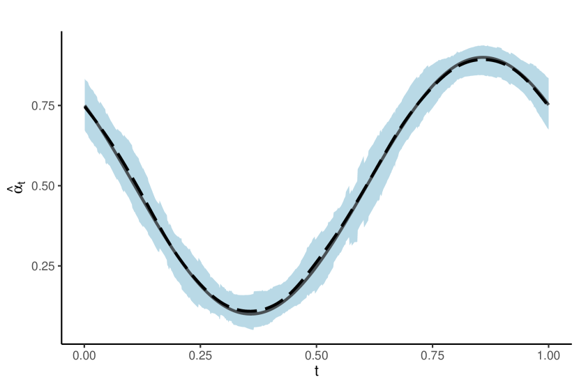
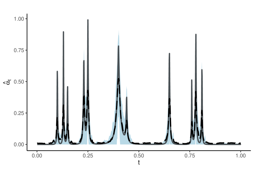
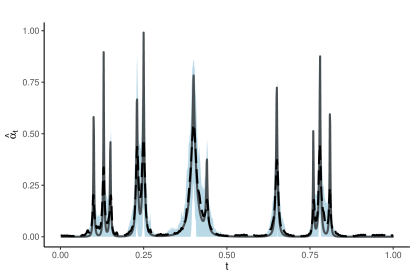
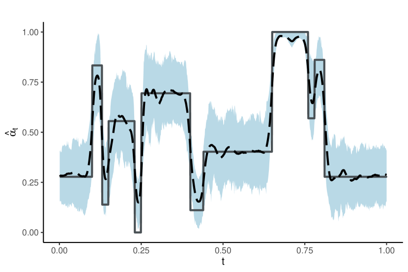
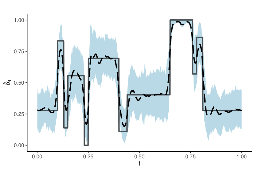
Figure 1: Estimates of the $\alpha_{t}$’s provided by SSG prior (left); and SSL prior (right). The curves assigned to $\alpha_{t}$ are, respectively: the sinusoidal (top), the bumps (middle), and the blocks (bottom). The full lines correspond to the $\alpha_{t}$’s curve, the dashed lines correspond to the average of the pointwise estimates and the shaded areas correspond to the 95% HPD intervals.

4.2 Taquari quota data set

Part of the Taquari-Antas Hydrographic Basin (TAHB) in the state of Rio Grande do Sul (south of Brazil), the Taquari River is located in the upper domain of the Baixo Taquari-Antas Valley, a region that has been affected by an increasing number of extreme rainfall events in recent decades (Tognoli et al.,, 2021). As a result, on many occasions, the rain excess is not drained efficiently and floods riverside regions. This phenomenon is aggravated in urban areas, where the human occupation of floodplains and the soil impermeability contribute to reducing the infiltration capacity and overloading the drainage system, leading to flood inundations (Kurek,, 2016).

As reported by Oliveira et al., (2018), Encantado is one of the cities adjacent to the course of the Taquari River most susceptible to fluvial inundations. The geomorphological and topographical characteristics of Encantado’s land favor the water accumulation and restrict its drainage (Oliveira et al.,, 2018). Furthermore, the urbanization of areas with high flood vulnerability in this municipality contributes to intensifying the occurrence of flood inundations (Kurek,, 2016).

Because of these circumstances, we propose implementing Algorithm 1 to a time series of Taquari’s river quota to estimate the probability of an inundation regime in Encantado’s urban areas. A river quota is the height of the water body, conventionally measured in centimeters (cm), on a given region of the riverbank. The data set corresponds to the records of Encantado´s fluviometric station identified by the code 86720000. The monthly time series of this station comes from the Hidroweb system, an integrated platform of the National Water Resources Management System (SINGREH) available at https://www.snirh.gov.br/hidroweb/serieshistoricas. Figure 2 shows a map of Encantado, highlighting the station used in this study.

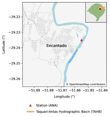
Figure 2: Location map of the fluviometric station in the city of Encantado. In the upper-right corner, the Taquari Antas Hydrographic Basin in Rio Grande do Sul state, south of Brazil.

To validate the estimated probabilities, we use a report from the Brazilian Geological Survey (CPRM) (Peixoto and Lamberty,, 2019) that records the months when floods occurred in Encantado. Therefore, we can see if the estimates of the mixture weight properly describe the flood regimes, no inundation and inundation, for each month. It is worth highlighting that since inundations can last for a couple of days or even more, there are no records of the specific days when these events took place, only the months. Because of that, and considering that the model is a mixture of two Gaussian distributions, we use the monthly average of the Taquari quota to estimate the probability associated with flood inundations. The period analyzed was from May 2004 to December 2014, consisting of 128 observations. Figure 3 presents this data set.

Table 3 shows the point estimates for the component parameters that describe each flood regime. Note that the results provided by the method under the SSG prior are similar to those achieved by it assigning the SSL prior to the distribution of wavelet coefficients. Concerning the dynamic mixture weights, Figure 4 shows the estimates considering both priors for $\bm{\theta}$. By analyzing the results, we see that using the SSL prior allows estimating higher peaks for the probabilities related to inundation periods than using the SSG prior. In fact, under a Bayes classifier, if the method employs the SSG prior, it can detect neither the months when flood episodes were reported nor change points ($\{t:\alpha_{t}=0.5\}$).

In summary, the method provides results consistent with the data on flood inundations in Encantado available in other works and reports (see Peixoto and Lamberty,, 2019, Tognoli et al.,, 2021). In addition, choosing the Laplace density in the spike and slab prior tends to provide dynamic weight estimates more capable of detecting floods.

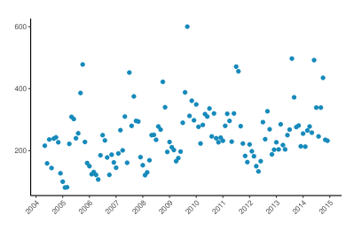
Figure 3: Monthly average of Taquari’s river quota (cm) from May 2004 to December 2014.

Table 3: Medians (95% HPD credible intervals) for the component parameters $\mu_{1},\tau_{1}^{2},\mu_{2}$ and $\tau_{2}^{2}$ of the Taquari quota data set, based on the MCMC samples.

Parameters	SSG prior	SSL prior
$\mu_{1}$	227.07 (210.09; 242.89)	220.60 (206.25; 236.28)
$\tau_{1}^{2}$	2.30e-4 (1.54e-4; 3.15e-4)	2.58e-4 (1.77e-4; 3.45e-4)
$\mu_{2}$	405.01 (316.38; 483.35)	400.20 (355.72; 439.54)
$\tau_{2}^{2}$	1.14e-4 (2.56e-5; 3.42e-4)	1.04e-4 (3.65e-5; 1.85e-4)

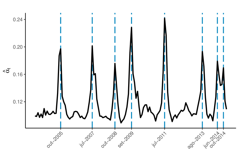
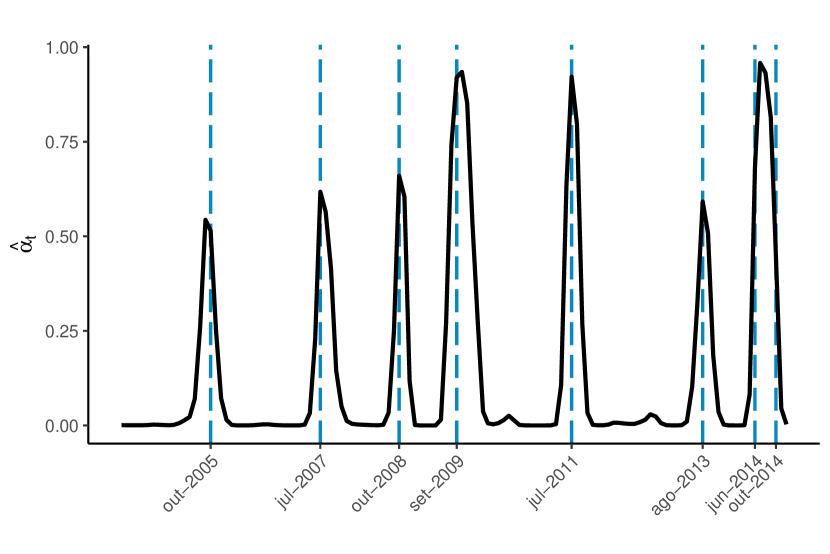
Figure 4: Estimates of the $\alpha_{t}$’s of the Taquari quota data provided by SSG prior (left); and SSL prior (right). The full (black) lines correspond to the point estimates (medians) and the dashed (blue) lines mark the months when flood inundations were reported by Peixoto and Lamberty, (2019).

5 Conclusion

This paper presents an approach to identify regime switches in bimodal data sets. We use a two-component mixture model whose mixture weight varies according to some index, like time. This adaptation makes the model more flexible and adaptive to a broader range of clustering and classification problems. Furthermore, we use wavelet bases to estimate the dynamic behavior of the mixture weight due to their excellent properties when it comes to curves’ estimation. However, unlike other approaches in the literature that also rely on wavelets (see Montoril et al.,, 2019), here we consider a Bayesian framework and propose estimating the dynamic weights and the component parameters jointly through an efficient Gibbs sampling algorithm.

We analyze the performance of this MCMC algorithm by conducting Monte Carlo experiments and illustrate the approach with an application to a river quota data set. Results from the simulations show that the method provides good estimates for the component parameters and the dynamic weights even when the function behind $\alpha_{t}$’s behavior is rougher. Additionally, the estimation performance using SSG prior is similar to the performance achieved when SSL prior is employed. The same does not apply to the results obtained in the river quota data set. For this application, we notice that implementing the method under the SSG prior to the wavelet coefficients yields smaller values for the probabilities associated with inundations occurrence than the estimates provided by using the SSL prior. This is likely because the Gaussian distribution does not have heavy tails, unlike the Laplace distribution.

References

- Abramovich et al., (2000) Abramovich, F., Bailey, T. C., and Sapatinas, T. (2000). Wavelet analysis and its statistical applications. Journal of the Royal Statistical Society: Series D (The Statistician), 49(1):1–29.
- Abramovich et al., (1998) Abramovich, F., Sapatinas, T., and Silverman, B. W. (1998). Wavelet thresholding via a bayesian approach. Journal of the Royal Statistical Society. Series B (Statistical Methodology), 60(4):725–749.
- Albert and Chib, (1993) Albert, J. H. and Chib, S. (1993). Bayesian analysis of binary and polychotomous response data. Journal of the American Statistical Association, 88(422):669–679.
- Bordes et al., (2006) Bordes, L., Delmas, C., and Vandekerkhove, P. (2006). Semiparametric estimation of a two-component mixture model where one component is known. Scandinavian Journal of Statistics, 33(4):733–752.
- Cai and Brown, (1999) Cai, T. and Brown, L. D. (1999). Wavelet estimation for samples with random uniform design. Statistics & Probability Letters, 42(3):313–321.
- (6) Donoho, D. L. (1993a). Nonlinear wavelet methods for recovery of signals, densities, and spectra from indirect and noisy data. In In Proceedings of Symposia in Applied Mathematics, pages 173–205. American Mathematical Society.
- (7) Donoho, D. L. (1993b). Unconditional bases are optimal bases for data compression and for statistical estimation. Applied and Computational Harmonic Analysis, 1(1):100–115.
- Donoho et al., (1996) Donoho, D. L., Johnstone, I. M., Kerkyacharian, G., and Picard, D. (1996). Density estimation by wavelet thresholding. The Annals of Statistics, 24(2):508–539.
- Donoho and Johnstone, (1994) Donoho, D. L. and Johnstone, J. M. (1994). Ideal spatial adaptation by wavelet shrinkage. Biometrika, 81(3):425–455.
- Escobar and West, (1995) Escobar, M. D. and West, M. (1995). Bayesian density estimation and inference using mixtures. Journal of the American Statistical Association, 90(430):577–588.
- George and McCulloch, (1993) George, E. I. and McCulloch, R. E. (1993). Variable selection via gibbs sampling. Journal of the American Statistical Association, 88(423):881–889.
- Hall and Patil, (1995) Hall, P. and Patil, P. (1995). Formulae for mean integrated squared error of nonlinear wavelet-based density estimators. The Annals of Statistics, 23(3):905–928.
- Hall and Zhou, (2003) Hall, P. and Zhou, X.-H. (2003). Nonparametric estimation of component distributions in a multivariate mixture. The Annals of Statistics, 31(1):201–224.
- Härdle et al., (2012) Härdle, W., Kerkyacharian, G., Picard, D., and Tsybakov, A. (2012). Wavelets, approximation, and statistical applications, volume 129. Springer Science & Business Media.
- Hughes and Guttorp, (1994) Hughes, J. P. and Guttorp, P. (1994). A class of stochastic models for relating synoptic atmospheric patterns to regional hydrologic phenomena. Water Resources Research, 30(5):1535–1546.
- Hui and Zhou, (1998) Hui, S. L. and Zhou, X.-H. (1998). Evaluation of diagnostic tests without gold standards. Statistical Methods in Medical Research, 7(4):354–370.
- (17) Johnstone, I. and Silverman, B. W. (2005a). Ebayesthresh: R programs for empirical bayes thresholding. Journal of Statistical Software, 12:1–38.
- (18) Johnstone, I. M. and Silverman, B. W. (2005b). Empirical bayes selection of wavelet thresholds. The Annals of Statistics, 33(4):1700–1752.
- Kurek, (2016) Kurek, R. K. M. (2016). Analysis of floods in the vale do taquari/rs as subsidy the development of a forecast model. Master’s thesis, Federal University of Santa Maria.
- Mallat, (1989) Mallat, S. G. (1989). A theory for multiresolution signal decomposition: the wavelet representation. IEEE transactions on pattern analysis and machine intelligence, 11(7):674–693.
- Montoril et al., (2021) Montoril, M. H., Correia, L. T., and Migon, H. S. (2021). Bayesian estimation of dynamic weights in gaussian mixture models.
- Montoril et al., (2019) Montoril, M. H., Pinheiro, A., and Vidakovic, B. (2019). Wavelet-based estimators for mixture regression. Scandinavian Journal of Statistics, 46(1):215–234.
- Morettin, (1996) Morettin, P. A. (1996). From fourier to wavelet analysis of time series. In Prat, A., editor, COMPSTAT, pages 111–122, Heidelberg. Physica-Verlag HD.
- Nagy et al., (2011) Nagy, I., Suzdaleva, E., Kárný, M., and Mlynářová, T. (2011). Bayesian estimation of dynamic finite mixtures. International Journal of Adaptive Control and Signal Processing, 25(9):765–787.
- Ogden, (1997) Ogden, R. T. (1997). Essential wavelets for statistical applications and data analysis. Birkhäuser Boston Inc.
- Oliveira et al., (2018) Oliveira, G. G. d., Eckhardt, R. R., Haetinger, C., and Alves, A. (2018). Caracterização espacial das áreas suscetíveis a inundações e enxurradas na bacia hidrográfica do rio taquari-antas. Geosciences= Geociências, 37(4):849–863.
- Patra and Sen, (2016) Patra, R. K. and Sen, B. (2016). Estimation of a two-component mixture model with applications to multiple testing. Journal of the Royal Statistical Society. Series B (Statistical Methodology), 78(4):869–893.
- Peixoto and Lamberty, (2019) Peixoto, C. A. B. and Lamberty, D. (2019). Setorização de áreas de alto e muito alto risco a movimentos de massa, enchentes e inundações: Encantado, rio grande do sul. Technical report, CPRM, Porto Alegre.
- Percival and Walden, (1999) Percival, D. B. and Walden, A. T. (1999). Wavelet Methods for Time Series Analysis. Cambridge Series in Statistical and Probabilistic Mathematics. Cambridge University Press.
- Priestley, (1996) Priestley, M. B. (1996). Wavelets and time-dependent spectral analysis. Journal of Time Series Analysis, 17(1):85–103.
- Richardson and Green, (2002) Richardson, S. and Green, P. J. (2002). On Bayesian Analysis of Mixtures with an Unknown Number of Components (with discussion). Journal of the Royal Statistical Society: Series B (Methodological), 59(4):731–792.
- Rindskopf and Rindskopf, (1986) Rindskopf, D. and Rindskopf, W. (1986). The value of latent class analysis in medical diagnosis. Statistics in Medicine, 5(1):21–27.
- Tognoli et al., (2021) Tognoli, F. M. W., Bruski, S. D., and Araujo, T. P. d. (2021). Data analysis reveals that extreme events have increased the flood inundations in the taquari river valley, southern brazil. Latin American Data in Science, 1(1):16–25.
- Vidakovic, (1999) Vidakovic, B. (1999). Statistical modeling by wavelets, volume 503. John Wiley & Sons.
- Walker et al., (2009) Walker, M. G., Mateo, M., Olszewski, E. W., Sen, B., and Woodroofe, M. (2009). Clean kinematic samples in dwarf spheroidals: An algorithm for evaluating membership and estimating distribution parameters when contamination is present. The Astronomical Journal, 137(2):3109.