Triaxial projected shell model approach for negative parity states in even-even nuclei

Abstract

The triaxial projected shell model (TPSM) approach is generalized to investigate the negative parity band structures in even-even systems. In the earlier version of the TPSM approach, the quasiparticle excitations were restricted to one major oscillator shell and it was possible to study only positive parity states in even-even systems. In the present extension, the excited quasiparticles are allowed to occupy two major oscillator shells, which makes it possible to generate the negative parity states. As a major application of this development, the extended approach is applied to elucidate the negative parity high-spin band structures in ^102-112Ru and it is shown that energies obtained with neutron excitation are slightly lower than the energies calculated with proton excitation. However, the calculated aligned angular momentum ($i_{x}$) clearly separates the two spectra with neutron $i_{x}$ in reasonable agreement with the empirically evaluated $i_{x}$ from the experimental data, whereas proton $i_{x}$ shows large deviations. Furthermore, we have also deduced the transition quadrupole moments from the TPSM wavefunctions along the negative-parity yrast- and yrare- bands and it is shown that these quantities exhibit rapid changes in the bandcrossing region.

I Introduction

To characterize the rich band structures observed in atomic nuclei is one of the main research themes in nuclear structure physics [1, 2]. Major advancements in the experimental techniques have made it feasible to populate multiple high-spin band structures, and in some nuclei more than fifty band structures have been reported [3, 4]. The description of this wealth of nuclear structure information is a major challenge to nuclear structure models [5]. In recent years, tremendous progress has been made in the spherical shell model (SSM) description of the nuclear properties [6, 7, 8]. It is now possible to apply SSM approach to medium mass nuclei, but studying high-spin band structures in heavy-mass region is still beyond the scope of this microscopic model. To describe the high-spin band structures, it is imperative to include, atleast, two-major oscillator shells as aligning particles occupy the high-j intruder orbitals. To perform the SSM calculations with two-major oscillator shells for heavier nuclei is beyond the reach of computational resources presently available [9].

On the other hand, although several major oscillator shells are considered in density functional approaches, but most of the calculations are restricted to investigate the ground-state properties only [10]. In order to study the high-spin band structures, the angular-momentum projection is required to be performed from the intrinsic mean-field state [11]. However, this approach is plagued with the singularity problem due to the reason that most of the modern energy density functionals are fitted to the experimental data with fractional density dependence and employ different forces in particle-hole and particle-particle channels [12, 13, 14]. It is to be added that in some recent works [15, 16, 17], the angular-momentum projection has also been performed in density functional theory (DFT) with projection after variation and the singularity problem does not appear to show up in these studies. However, it has been discussed in Ref. [10] that projected results will contain spurious components that need to be examined.

Considering the above problems associated with the SSM and DFT approaches, triaxial projected shell model (TPSM) approach has become a tool of choice to investigate the high-spin band structures in well deformed and transitional nuclei [18, 19, 20, 21, 22]. The advantage of this approach is that computational resources involved are quite modest and it is possible to perform a systematic study of a large set of atomic nuclei. As a matter of fact, several systematic investigations have been performed for chiral, wobbling and $\gamma$-vibrational band structures observed in triaxial nuclei [5, 23, 19, 20, 21, 22, 5, 24]. The model space in the TPSM approach is spanned by multi-quasiparticle basis states which allows to investigate high-spin band structures. In the original version of the TPSM approach, the model space was quite limited [18] but in recent applications [22, 20, 19, 23, 25], we have generalized the basis space to include higher order quasiparticle states. For instance, for even-even systems [22], the TPSM approach has been generalized to include four-neutron and four-proton quasiparticle basis states. This extension allows to investigate the high-spin properties in even-even systems beyond the second band crossing.

Nevertheless, in all the extended versions of the TPSM approach the basis configurations are constructed from one major oscillator shell only, although the vacuum configuration is generated from all the three major shells considered in the model. The justification is that the aligning particles occupy high-j intruder subshell and in order to describe band crossing, it is sufficient to consider quasiparticle excitations only from one major shell containing the intruder orbital.

For even-even systems, the restriction of the quasiparticle excitations from one oscillator shell gives rise to only positive parity states and in order to generate the negative parity states, the quasiparticle excitations need to be considered from two oscillator shells having different parities for the single-particle states. The purpose of the present work is to develop the generalized TPSM approach with the quasiparticle excitations from two major oscillator shells. There is a considerable data available for negative parity bands in even-even systems [26, 27, 28, 29, 30, 31, 32, 33, 34]. However, there have been very limited theoretical calculations to investigate these band structures.

In the present work, we shall focus on the application of the new development to neutron-rich nuclei around A $\sim$ 110. The properties of these nuclei are studied by measuring prompt $\gamma$-rays emitted by secondary fragments produced by spontaneous and induced fission of ²⁵²Cf source [26, 35]. The weak transitions in the excited negative parity bands are identified through triple and higher order coincidence techniques [36] using the state-of-the-art detector arrays. The ground-state positive parity bands in this region are known to have strong prolate shapes [37], and the negative parity doublet bands identified in some nuclei are proposed to originate from chiral symmetry breaking mechanism [26]. In our earlier publications, we have studied the positive parity bands in this mass region [25, 23, 38] using the TPSM approach and in the present work, we shall focus on the negative parity band structures. Some preliminary results of the present approach for the observed negative parity band structures in ^106,108Mo were published with the experimental group [39]. However, in this work only neutron-excitation were considered. In the present work, both neutron- and proton-excitations are included in the model space. The remaining manuscript is organized in the following manner. In the next section, we provide a few details of the extended TPSM approach for negative parity bands and some explicit expressions of the matrix elements are included in the appendix. In section III, the results obtained for Ru-isotopes are presented and discussed, and finally the present work is summarized in section IV.

Table 1: Axial and triaxial quadrupole deformation parameters $\epsilon$ and $\gamma=\textrm{tan}^{-1}{(\epsilon^{\prime}/\epsilon)}$ employed in the TPSM calculation. Axial deformations $\epsilon$ have been considered from [40] with some adjustment as discussed in the text. The nonaxial values ($\gamma$) are chosen in such a way that observed data is reproduced.

	102Ru	104Ru	106Ru	108Ru	110Ru	112Ru
$\epsilon$	0.220	0.270	0.280	0.275	0.275	0.270
$\gamma$	30∘	26 ∘	25∘	26∘	30∘	30∘

II Triaxial Projected Shell Model Approach

TPSM approach is similar to the SSM technique with the difference that deformed basis are used instead of the spherical one’s [18, 41]. The deformed basis are the optimum basis states to study deformed nuclei, and in the TPSM approach these are generated by solving the three-dimensional Nilsson mean-field potential [42]. The pairing interaction is then considered in the Bardeen-Cooper-Scrieffer (BCS) approximation [11]. The Nilsson + BCS wavefunctions thus constructed form the basis configuration in the TPSM approach. The vacuum state is then constructed by considering valence neutrons and protons to occupy three major oscillator shells [18]. However, the quasiparticle excitations are considered from one major oscillator shell only. For instance, to investigate the high-spin band structures in mass $\sim$ 110 region, quasiproton (quasineutron) excitations are considered from the N = 4 (5) shells which contain the $1g_{9/2}(1h_{11/2})$ shell that is responsible for proton (neutron) alignments in this region. This restriction allows to study only positive parity band structures in even-even systems and in order to describe the negative parity band structures, valence pair of particles need to be placed in two different oscillator shells having opposite parities.

In the present work, we have generalized the TPSM approach with valence neutrons and protons occupying different shells. The extended basis space is composed of:

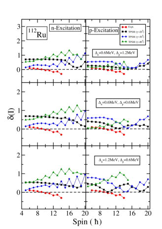
Figure 1: (Color online) Energy difference between negative-parity yrast- and yrare- bands for same spin, $I$, $\delta(I)=(E_{2}(I)-E_{1}(I))$ in ¹¹²Ru.

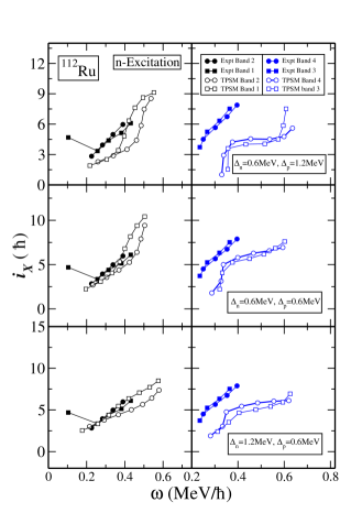
Figure 2: (Color online) Comparison of the aligned angular momenta, $i_{X}=i_{x}(\omega)-i_{x,ref}(\omega)$, where $\hbar\omega=\frac{E_{\gamma}}{I^{i}_{x}(\omega)-I^{f}_{x}\omega}$,$I_{x}\omega=\sqrt{I(I+1)-K^{2}}$ and $i_{x,ref}(\omega)=\omega(J_{0}+\omega^{2}J_{1})$. The reference band Harris parameters used are $J_{0}=14$ and $J_{1}=15$, obtained from the measured energy levels as well as those calculated from the TPSM results for neutron excitation in ¹¹²Ru.

$$\hat{P}^{I}_{MK}~{}a^{\dagger}_{n_{1}}a^{\dagger}_{n_{2}^{\prime}}|\Phi\rangle;$$

$$\hat{P}^{I}_{MK}~{}a^{\dagger}_{n_{1}}a^{\dagger}_{n_{2}^{\prime}}a^{\dagger}_{n_{3}^{\prime}}a^{\dagger}_{n_{4}^{\prime}}|\Phi\rangle;$$

$$\hat{P}^{I}_{MK}~{}a^{\dagger}_{n_{1}}a^{\dagger}_{n_{2}^{\prime}}a^{\dagger}_{p_{1}^{\prime}}a^{\dagger}_{p_{2}^{\prime}}|\Phi\rangle;$$

$$\hat{P}^{I}_{MK}~{}a^{\dagger}_{p_{1}}a^{\dagger}_{p_{2}^{\prime}}|\Phi\rangle;$$

$$\hat{P}^{I}_{MK}~{}a^{\dagger}_{p_{1}}a^{\dagger}_{p_{2}^{\prime}}a^{\dagger}_{p_{3}^{\prime}}a^{\dagger}_{p_{4}^{\prime}}|\Phi\rangle;$$

$$\hat{P}^{I}_{MK}~{}a^{\dagger}_{p_{1}}a^{\dagger}_{p_{2}^{\prime}}a^{\dagger}_{n_{1}^{\prime}}a^{\dagger}_{n_{2}^{\prime}}|\Phi\rangle,$$ (1)

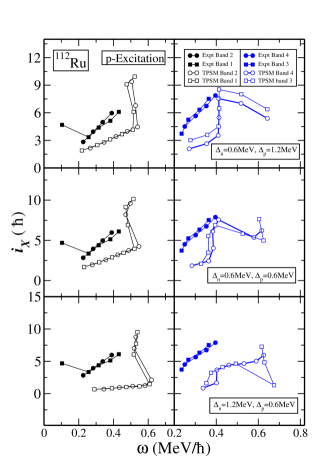
Figure 3: (Color online) Comparison of the aligned angular momenta, $i_{X}=i_{x}(\omega)-i_{x,ref}(\omega)$, where $\hbar\omega=\frac{E_{\gamma}}{I^{i}_{x}(\omega)-I^{f}_{x}\omega}$,$I_{x}\omega=\sqrt{I(I+1)-K^{2}}$ and $i_{x,ref}(\omega)=\omega(J_{0}+\omega^{2}J_{1})$. The reference band Harris parameters used are $J_{0}=14$ and $J_{1}=15$, obtained from the measured energy levels as well as those calculated from the TPSM results for proton excitation in ¹¹²Ru.

where the neutron (proton) major oscillator shells employed are designated by the quantum numbers $n$ ($p$) with neutrons (protons) occupying two different oscillator shells, $n(p)$ and $n^{\prime}(p^{\prime})$. We have considered excitations in both proton and neutron sectors, however, the separable interaction employed doesn’t mix these excitations and the two can be diagonalized separately. It is demonstrated in the appendix that matrix elements between neutron and proton excitations vanish.

It has been demonstrated that two-neutron and two-proton excitations are almost at the same energy [27], it is therefore necessary to consider both neutron and proton excitations in the TPSM basis. Further, two-neutron and two-proton aligning configurations have been added as negative parity bands in some nuclei that have been populated up to quite high-spin and the band crossing phenomena have been observed. $\,|\,\Phi\rangle$ in Eq. (1) is the quasiparticle vacuum state which has positive parity, and the three-dimensional angular-momentum projection operator, $\hat{P}^{I}_{MK}$, is given by [11, 43, 44]

$$\hat{P}^{I}_{MK}={2I+1\over 8\pi^{2}}\int~{}d\Omega\,D^{I}_{MK}(\Omega)\,\hat{R}(\Omega),$$ (2)

with the rotation operator

$$\hat{R}(\Omega)=e^{-\imath\alpha\hat{J}_{z}}e^{-\imath\beta\hat{J}_{y}}e^{-\imath\gamma\hat{J}_{z}}~{}~{}~{}.$$ (3)

Here, ${}^{\prime\prime}\Omega^{\prime\prime}$ represents a set of Euler angles ($\alpha,\gamma=[0,2\pi],\,\beta=[0,\pi]$) and the $\hat{J}^{,}s$ are angular-momentum operators.

In the present work we have employed $N=3,4,5$ ($2,3,4$) for neutrons (protons). The two valence neutrons (protons) are occupying N= 4 (3) and 5 (4) shells that give rise to the negative parity states. The deformations used to generate the Nilsson basis configuration are given in Table 1 and have been adopted from earlier works [25, 38, 40]. The Nilsson intrinsic states are then projected onto the states with good angular-momentum through three-dimensional projection.

Figure 4: (Color online) Comparison of the aligned angular momenta, $i_{X}=i_{x}(\omega)-i_{x,ref}(\omega)$, where $\hbar\omega=\frac{E_{\gamma}}{I^{i}_{x}(\omega)-I^{f}_{x}\omega}$,$I_{x}\omega=\sqrt{I(I+1)-K^{2}}$ and $i_{x,ref}(\omega)=\omega(J_{0}+\omega^{2}J_{1})$. The reference band Harris parameters used are $J_{0}=14$ and $J_{1}=15$, obtained from the measured energy levels as well as those calculated from the TPSM results for neutron excitation in ¹¹²Ru.

The projected basis states of Eq. (1) are then used to diagonalize the shell model Hamiltonian. As in our earlier studies, we have employed the pairing plus quadrupole-quadrupole Hamiltonian [24, 45]

$$\hat{H}=\hat{H}_{0}-{1\over 2}\chi\sum_{\mu}\hat{Q}^{\dagger}_{\mu}\hat{Q}_{\mu}-G_{M}\hat{P}^{\dagger}\hat{P}-G_{Q}\sum_{\mu}\hat{P}^{\dagger}_{\mu}\hat{P}_{\mu}.$$ (4)

The corresponding triaxial Nilsson Hamiltonian is the mean-field of the above model Hamiltonian and is given by:

$$\hat{H}_{N}=\hat{H}_{0}-{2\over 3}\hbar\omega\left\{\epsilon\hat{Q}_{0}+\epsilon^{\prime}{{\hat{Q}_{+2}+\hat{Q}_{-2}}\over\sqrt{2}}\right\}.$$ (5)

In the above equation, $\hat{H}_{0}$ is the spherical single-particle Nilsson Hamiltonian [46]. The monopole pairing strength $G_{M}$ of the standard form

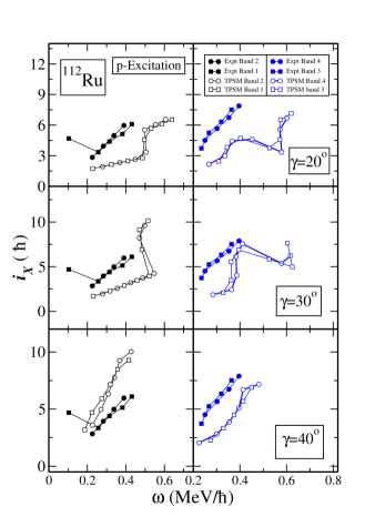
Figure 5: (Color online) Comparison of the aligned angular momenta, $i_{X}=i_{x}(\omega)-i_{x,ref}(\omega)$, where $\hbar\omega=\frac{E_{\gamma}}{I^{i}_{x}(\omega)-I^{f}_{x}\omega}$,$I_{x}\omega=\sqrt{I(I+1)-K^{2}}$ and $i_{x,ref}(\omega)=\omega(J_{0}+\omega^{2}J_{1})$. The reference band Harris parameters used are $J_{0}=14$ and $J_{1}=15$, obtained from the measured energy levels as well as those calculated from the TPSM results for proton excitation in ¹¹²Ru.

$$G_{M}={{(G_{1}\mp G_{2}{{N-Z}\over A})}\frac{1}{A}}(MeV).$$ (6)

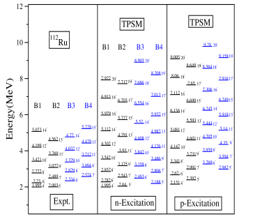
Figure 6: (Color online) TPSM projected energies after configuration mixing for both neutron- and proton-excitations are compared with experimental data [26] for ¹¹²Ru isotope.

In the present calculation, we considered $G_{1}=22.68$ and $G_{2}=16.22$, which approximately reproduce the observed odd-even mass difference in the studied mass region. The quadrupole pairing strength $G_{Q}$ is assumed to be proportional to $G_{M}$, and the proportionality constant being fixed as 0.18. These interaction strengths are consistent with those used earlier for the same mass region [38, 47].

The projected TPSM wavefunction is then given by

$$|\sigma,IM\rangle=\sum_{K\kappa}f^{\sigma}_{K\kappa}\hat{P}^{I}_{MK}|\phi_{\kappa}\rangle.$$ (7)

Here, the index $\sigma$ labels the states with same angular momentum and $\kappa$ the basis states. In Eq. (7), $f^{\sigma}_{K\kappa}$ are the expansion coefficients of the wavefunction in terms of the non-orthonormal projected basis states, $\hat{P}^{I}_{MK}|\phi_{\kappa}\rangle$. These coefficients are not probability amplitudes in the usual quantum mechanical sense and in the work of ref. [48], modified expansion coefficients $(g^{\sigma}_{K\kappa})$ are defined which are expanded in terms of an orthonormal basis set in the following manner :

$$g^{\sigma}_{K\kappa}=\sum_{K^{\prime}\kappa^{\prime}}f^{\sigma}_{K^{\prime}\kappa^{\prime}}\langle K\kappa|\hat{P}^{I}_{MK^{\prime}}|\phi_{\kappa^{\prime}}\rangle=\sum_{K^{\prime}\kappa^{\prime}}f^{\sigma}_{K^{\prime}\kappa^{\prime}}N^{1/2}_{K\kappa K^{\prime}\kappa^{\prime}}$$ (8)

where $N$ is the norm matrix and $|K\kappa\rangle$ is an orthonormal basis set.

Finally, the minimization of the projected energy with respect to the expansion coefficient, $f^{\sigma}_{K\kappa}$, leads to the Hill-Wheeler type equation

$$\sum_{\kappa^{\prime}}(H_{\kappa\kappa^{\prime}}-E_{\sigma}N_{\kappa\kappa^{\prime}})f^{\sigma}_{K\kappa^{\prime}}=0,$$ (9)

where the normalization is chosen such that

$$\sum_{\kappa\kappa^{\prime}}f^{\sigma}_{K\kappa}N_{\kappa\kappa^{\prime}}f^{\sigma^{\prime}}_{K\kappa^{\prime}}=\delta_{\sigma\sigma^{\prime}}.$$ (10)

The above equations are then solved to obtain the energies and the wavefunctions [41].

In the present work, we have also evaluated the transition probabilities using the TPSM wavefunctions with the effective charges of $0.5e$ and $1.5e$ for neutrons and protons. The details of the transition probability calculations with explicit expressions are given in the review article [5].

III Results and Discussion

In comparison to the positive parity bands, there have been only a few theoretical studies to investigate the negative parity bands in Ru-isotopes and other isotopes in the A $\sim$ 110 mass region. The band heads of the two-quasiparticle structures have been studied using the D1S Gogny force [27], and it has been discussed that two-proton and two-neutron bands for Ru-isotopes are at a similar excitation energy of about 2 MeV. In the self-consistent constrained cranking Skyrme calculations with particle number conserving pairing [49], it has been shown that calculated moments of inertia of two-neutron quasiparticle configuration are in better agreement with the experimental data as compared to the two-proton configuration for ^108,110,112Ru isotopes, and the observed bands have been characterized as neutron excited bands.

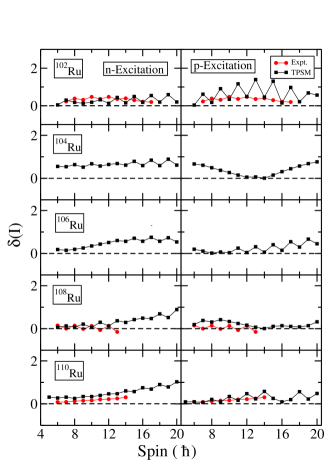
Figure 7: (Color online) Energy difference between negative-parity yrast- and yrare- bands for same spin, $I$, $\delta(I)=(E_{2}(I)-E_{1}(I))$ in ^{102,104,106,108,110}Ru.

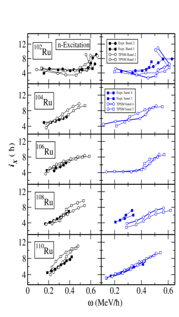
Figure 8: (Color online) Comparison of the aligned angular momenta, $i_{X}=i_{x}(\omega)-i_{x,ref}(\omega)$, where $\hbar\omega=\frac{E_{\gamma}}{I^{i}_{x}(\omega)-I^{f}_{x}\omega}$,$I_{x}\omega=\sqrt{I(I+1)-K^{2}}$ and $i_{x,ref}(\omega)=\omega(J_{0}+\omega^{2}J_{1})$. The reference band Harris parameters used are $J_{0}=14$ and $J_{1}=15$, obtained from the measured energy levels as well as those calculated from the TPSM results for neutron excitation in ^{102,104,106,108,110}Ru.

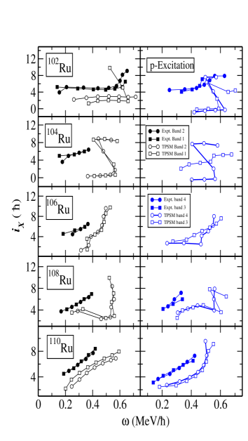
Figure 9: (Color online) Comparison of the aligned angular momenta, $i_{X}=i_{x}(\omega)-i_{x,ref}(\omega)$, where $\hbar\omega=\frac{E_{\gamma}}{I^{i}_{x}(\omega)-I^{f}_{x}\omega}$,$I_{x}\omega=\sqrt{I(I+1)-K^{2}}$ and $i_{x,ref}(\omega)=\omega(J_{0}+\omega^{2}J_{1})$. The reference band Harris parameters used are $J_{0}=14$ and $J_{1}=15$, obtained from the measured energy levels as well as those calculated from the TPSM results for proton excitation in ^{102,104,106,108,110}Ru.

In order to perform the TPSM study of the negative parity bands, the input parameters required are deformation values and the strengths of the monopole and the quadrupole pairing interaction terms. It is expected that deformation of the negative parity two-quasiparticle states will be slightly different from the yrast positive parity band structures. However, in the absence of any systematic study of the deformation properties of these band structures, we have adopted the axial deformation values of the ground-state bands from theoretical studies using microscopic-macroscopic model predictions [40] with slight adjustments as in our previous studies [5, 39]. The non-axial deformation values have been varied to reproduce the observed properties of these bands. The deformation values adopted in the present analysis are listed in Table 1.

The pairing parameters are clearly expected to be different from the ground-state values as these are two-quasiparticle states, and it is known that pairing is reduced for the excited quasiparticle states. However, it is difficult to study the reduction in the pairing correlations for the quasiparticle states as in the BCS approximation, the pairing collapses for the blocked states and it is imperative to perform the particle-number projected analysis before variation [50]. In the present work, we have investigated the sensitivity of the results on the pairing correlations by varying the monopole pairing strengths.

We have considered ¹¹²Ru as an illustrative example to investigate the deformation and pairing dependence of the TPSM results. The pairing strength parameters that best reproduce the experimental data of ¹¹²Ru are then used to perform the TPSM calculations for other Ru-isotopes from A=102 to 110. The reason that this system has been chosen is because doublet band structures have been observed for this nucleus up to quite high-spin and the system is well deformed [26]. For other isotopes, for instance, ¹⁰²Ru the data is also available up to quite high-spin. However, this system has vibrational character in the low-spin region [28] and the application of TPSM approach becomes unreliable as a single deformed mean-field solution is adopted in this model.

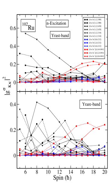
Figure 10: (Color online) Probabilities of various projected K configurations in the orthonormal wavefunctions of the negative-parity yrast- and yrare- bands after diagonalization for ¹⁰²Ru. The curves are labeled by three quantities: quasiparticle character, ^′′K^′′ quantum number and energy of the quasiparticle state. For instance, [($1\text{n}1\text{n}^{\prime})$,$3$,$2.3$] designates two–quasineutron state with K$=3$ having intrinsic energy of $2.3$ MeV. Even- and odd-spin states correspond to $\alpha=0$ (solid lines) and $\alpha=1$ (dashed lines), respectively.

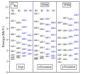
Figure 11: (Color online) TPSM projected energies after configuration mixing for both neutron- and proton-excitations are compared with experimental data [28] for ¹⁰²Ru isotope.

It has been proposed that the doublet band structures observed in ¹¹²Ru originate from the chiral symmetry breaking mechanism [26] as the difference of the energies between the two bands, $\delta(I)=(E_{2}(I)-E_{1}(I))$, is very small. In Fig. 1, this difference is plotted for different values of pair-gaps ($\Delta$) and non-axial deformation. The differences in the excitation energies of both two-neutron (left panel) and two-proton (right panel) quasiparticle configurations are plotted. The results are depicted only for three representative values of the pair-gaps, $\Delta_{n}=0.6~{}\textrm{MeV},~{}\Delta_{p}=1.2~{}\textrm{MeV}$;  $\Delta_{n}=0.6~{}\textrm{MeV},~{}\Delta_{p}=0.6~{}\textrm{MeV}$ and $\Delta_{n}=1.2~{}\textrm{MeV},~{}\Delta_{p}=0.6~{}\textrm{MeV}$. [ The TPSM calculations have also been performed for other values of the pair-gaps between 0.6 and 1.2, and the results are not very different from the three cases depicted in Fig. 1]. It is evident from the results that $\gamma=30^{0}$ leads to lowest differences in the energies and agrees with the corresponding experimental numbers. Further, the results with the pairing set of $\Delta_{n}=\Delta_{p}=0.6$ MeV appears to be in better agreement with the data for the neutron excitation case as compared to the proton excitation.

To further examine the optimum pairing set and the non-axial deformation parameter that reproduce the experimental data more accurately, we have evaluated the aligned angular momentum values, $i_{x}$, for the doublet bands and the results are presented in Figs. 2, 3, 4 and 5. As compared to the energies, $i_{x}$ is sensitive to the single-particle states occupied by the excited particles and should provide a better estimate of the optimum pairing and deformation set. The calculated $i_{x}$ for the neutron excited configuration are shown in Fig. 2 for three different pairing sets, but with the same non-axial deformation parameter of $\gamma=30^{\circ}$. It is evident from the figure that the pairing set of $\Delta_{n}=\Delta_{p}=0.6~{}\textrm{MeV}$ provides a better representation of the experimental values as compared to the other two sets, in particular, $i_{x}$ for Bands 1 and 2 is reproduced remarkably well with this set. Further, the slope of the alignment curve, which is the moment of inertia, is also in good agreement with the data for this set. The alignment calculated with the proton excitation is depicted in Fig. 3 and it is noted that none of the parameter set is able to reproduce the experimental values. The calculated $i_{x}$ values depict backbending phenomena, whereas the experimental values show a smooth increase with spin for both the bands. In Figs. 4 and 5, the alignments are displayed for different values of the non-axial deformation parameters and with the pairing set of $\Delta_{n}=0.6~{}\textrm{MeV},~{}\Delta_{p}=0.6~{}\textrm{MeV}$. It is evident from these figures that $\gamma=30^{\circ}$ for the neutron excitation shows the best agreement with the data.

The lowest two negative parity bands obtained for ¹¹²Ru after diagonalization of the shell model Hamiltonian, for both neutron and proton excitations, are compared with the experimental energies in Fig. 6. It has been already stated that TPSM Hamiltonian, in the absence of the exchange terms, does not mix neutron and proton excitations and the two basis spaces can be diagonalized separately. The calculated band structures obtained with the neutron excitation are lower in energy as compared to the band structures with the proton excitation. The lowest negative band structure (labelled as B1 and B2 in Fig. 6) is quite reasonably reproduced by the TPSM calculations with neutron excitation, and the deviation for the highest spin, I=14, for this band is 0.039 MeV. For the excited band (labelled as B3 and B4), significant deviations are noted for most of the spin states and for the highest spin observed, I=15, the calculated value has a deviation of 0.704 MeV.

The alignment plotted in Fig. 2 also depicts significant deviations, although the slope is in agreement. The origin of this deviation is not evident at this stage and further analysis is needed, for instance, using a self-consistent mean-field approach. In Fig. 6, we have also provided the energies of the proton excited bands as in future experimental studies more band structures will be populated and some of them may correspond to the proton excitation.

It needs to be mentioned that TPSM energies in Fig. 6 have been plotted for lower-spin values as well, which are not known experimentally. The reason is that the studied negative-parity band structures have dominant K=2 and 3 configurations as is evident from the TPSM wavefunctions and, therefore, the band structures will have either I=2 or 3 as bandheads. The yrast negative-parity band has been plotted from the spin-value observed in the experimental data as calculated TPSM energy for this state is set equal to the corresponding experimental value. For the negative-parity yrare-band, we have also provided a few low-lying states which are not known experimentally. The reason that these low-lying states are not known is probably because these are mixed with spherical states as many negative parity states are observed in these nuclei which are not members of the rotational bands.

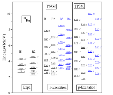
Figure 12: (Color online) TPSM projected energies after configuration mixing for both neutron- and proton-excitations are compared with experimental data [27] for ¹⁰⁴Ru isotope.

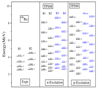
Figure 13: (Color online) TPSM projected energies after configuration mixing for both neutron- and proton-excitations are compared with experimental data [27] for ¹⁰⁶Ru isotope.

Figure 14: (Color online) TPSM projected energies after configuration mixing for both neutron- and proton-excitations are compared with experimental data [26] for ¹⁰⁸Ru isotope.

We have performed TPSM study for other Ru-isotopes from A=102 to 110 with the axial and non-axial deformation values listed in Table 1. The pairing strengths are same as those adjusted to reproduce the properties of ¹¹²Ru. The results of the energy difference between the two doublet band, $\delta(I)$, are displayed in Fig. 7 for both proton and neutron excitations. Neutron excitation energies are slightly lower than the corresponding proton energies, however, both are compared with the available experimental data as the proton excitation spectra can become favoured with slight adjustments in the pairing and deformation parameters. It is noticed from the figure that TPSM calculated $\delta(I)$ from neutron excitation energies agrees well with the observed energies of ¹⁰²Ru, ¹⁰⁸Ru and ¹¹⁰Ru. It is also evident from the figure that $\delta(I)$ for the lowest two proton bands also agrees with the data, except for ¹⁰²Ru which shows a staggering pattern. For other isotopes yrare-band has not been observed.

The alignments of the isotopes are plotted in Fig. 8 for neutron excitation spectra and compared with the corresponding experimental numbers, wherever available. It is quite remarkable to note from the figure that $i_{x}$ values are reproduced well for all the isotopes. For ¹⁰²Ru, upbend is observed for bands B1 and B2 at $\hbar\omega\approx 0.55$ MeV and is well described by the TPSM calculations. For other isotopes, $i_{x}$ depicts a smooth increase with rotational frequency and is easily understood as unpaired particles align towards the rotational axis. For ¹⁰⁶Ru, TPSM calculated bands B3 and B4 show upbends, but there is no experimental data to confirm this band crossing phenomenon. The alignments for the proton excitation bands are displayed in Fig. 9 and it is noted that in most of the cases, the band crossing is expected as either an upbend or a backbend is observed. These alignments considerably differ with the experimental values.

To examine the nature of the bandcrossing phenomenon observed in ¹⁰²Ru, the wavefunction probabilities are displayed in Fig. 10 for both negative-parity yrast- and yrare- bands. It is noted from the figure that for the negative-parity yrast-band, the dominant component before I=14 is a mixture of many $(1n1n^{\prime})$ configurations. After I=14, the dominant component in the wavefunction is a four quasiparticle state, $(1n1n^{\prime}2p^{\prime})$ having K=2, which is a two-proton aligned state built on the basic $(1n1n^{\prime})$ configuration. It is observed from Fig. 10 that there is a considerable mixing between the two-quasiparticle and the proton-aligned four-quasiparticle states and, therefore, upbend rather than a backbend is expected and this is what is seen in the alignment plot for ¹⁰²Ru in Fig. 8. For the negative-parity yrare-band, bandcrossing is also expected at I=14 as the wavefunction in the lower panel of Fig. 10 depicts dominant $(1n1n^{\prime})$ contribution before this spin value and after it, the wavefunction is dominated by $(1n1n^{\prime}2p^{\prime})$ four-quasiparticle state with K=4.

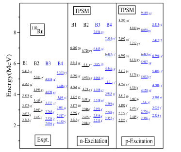
Figure 15: (Color online) TPSM projected energies after configuration mixing for both neutron- and proton-excitations are compared with experimental data [26] for ¹¹⁰Ru isotope.

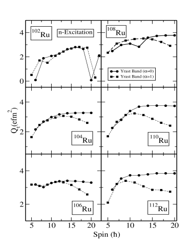
Figure 16: (Color online) TPSM calculated transition quadrupole moments, $Q_{t}(e\textrm{fm}^{2})$, for the negative-parity yrast-band in ^102-112Ru isotopes.

TPSM calculated energy spectra are compared with the experimental energies in Figs. 11, 12, 13, 14 and 15 for ¹⁰²Ru,¹⁰⁴Ru, ¹⁰⁶Ru, ¹⁰⁸Ru and ¹¹⁰Ru, respectively. For ¹⁰²Ru, the experimental energies are known up to I=23, and it is observed that TPSM calculations with neutron excitation reproduces the data quite well, the deviations for most of the states is less than 0.2 MeV. The proton excitation bands at low-spin are almost degenerate with the neutron bands, but at higher spins, they become unfavoured. In the case of ¹⁰⁴Ru and ¹⁰⁶Ru, the data is available up to I=13 and only one band is known. The TPSM results are in reasonable agreement with the data for both the nuclei. For ¹⁰⁸Ru and ¹¹⁰Ru, doublet negative parity bands have been observed and it is noted that TPSM calculation are able to reproduce the low-lying states in both the nuclei quite well, however, deviations are noted for the excited states.

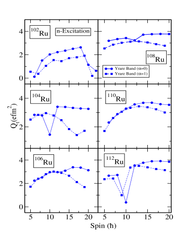
Figure 17: (Color online) TPSM calculated transition quadrupole moments, $Q_{t}(e\textrm{fm}^{2})$, for the negative parity yrare-band in ^102-112Ru isotopes.

As transition probabilities are more sensitive to any structural changes, we have also evaluated the transition quadrupole moment ($Q_{t}$) for the negative-parity yrast- and yrare- bands for all the studied isotopes and the results are presented in Figs. 16 and 17. It is evident from the figures that in the bandcrossing region, $Q_{t}$ depicts large changes since the wavefunctions are mixed in this region. For ¹⁰²Ru, the drop is observed at I=20 and 21 for the two signature branches and these are the spin values for which large changes are oberved in the aligned angular momentum as seen from Fig. 8. It is noted from Fig. 17 that negative parity yrare-band for ¹¹²Ru also depicts a large drop at I=10 and substantiates the occurence of bandcrossing at this spin value with the aligned angular momenta showing a rapid increase in Fig. 2 for the corresponding angular frequency value.

IV Summary and Conclusions

In the present work, the TPSM approach has been extended to investigate the negative parity bands in even-even systems. In all the previous versions of the model, the quasiparticle excitations were considered from a single oscillator shell and it was possible to investigate only positive parity bands. Here, we have extended the model space by considering quasiparticle basis from two different oscillator shells and a detailed investigation has been performed for the negative parity bands observed in ^102-112Ru as considerable data is available for these isotopes.

Both proton and neutron quasiparticle excitations have been considered in the present analysis and it has been observed that neutron spectra is slightly lower than the proton one. However, the comparison of alignments clearly delineated the two spectra with neutron alignment observed to be in better agreement with the data and proton alignment shows significant deviations. Further, transition quadrupole moments for both negative-parity yrast- and yrare- bands have been evaluated and it is noted that these depict large changes in the bandcrossing region.

In order to improve the predictive power of the present investigation, deformation and pairing parameters need to be determined for the negative parity bands. It is quite evident that parameters known for the yrast positive parity configurations cannot be used for the two-quasiparticle negative parity states. It is essential to deduce these parameters from the microscopic models, for instance, the energy density functional approaches with the blocking technique [51]. We are planning to perform this study using the Skyrme density functional approach [52] and these parameters will then be used to evaluate the properties of negative parity band structures more accurately and will allow us to investigate the chiral symmetry origin proposed for some of the studied isotopes.

In some of the nuclei studied, the octupole deformation is predicted to be an important degree of freedom [34, 28] and TPSM approach needs to be augmented to include the octupole deformation. We are considering to include the octupole correlations in the TPSM framework. This can be achieved in two phases. In the first phase, the octupole-octupole interaction will be included in the Hamiltonian with the mean-field having well defined parity. In this way, the octupole correlations will be added as a perturbation correction. In the second phase, the octupole mean-field will be considered in the Nilsson state with the explicit breaking of the reflection symmetry. This broken symmetry can then be restored using the standard parity projection formalism [53, 54, 55, 56].

Further, a major deficiency of the present approach is that deformation and pairing fields are kept fixed irrespective of the angular-momentum and quasiparticle configuration as the projection is carried out after variation. This is a gross simplification since it is known that mean-field is modified for multi-quasiparticle and higher angular-momentum states. It is highly desirable that generator coordinate method (GCM) [57, 58] be developed with the TPSM wavefunctions as basis configurations. In recent years, considerable progress has been made in the implementation of the GCM related techniques in nuclear physics and microscopic structure of various phenomena have been explored [59, 60, 61, 62, 63, 64].

Appendix

The Hamiltonian in terms of proton and neutron degrees of freedom employed in the TPSM approach is given by

$$\hat{H} =\hat{H}_{0}-{\chi_{pp}\over 2}\sum_{\mu}\hat{Q}^{\dagger}_{\mu}(p)\hat{Q}_{\mu}(p)-{\chi_{nn}\over 2}\sum_{\mu}\hat{Q}^{\dagger}_{\mu}(n)\hat{Q}_{\mu}(n)-\chi_{np}\sum_{\mu}\left(\hat{Q}^{\dagger}_{\mu}(p)\hat{Q}_{\mu}(n)+\hat{Q}^{\dagger}_{\mu}(n)\hat{Q}_{\mu}(p)\right)$$

$$-G_{M}^{p}\hat{P}^{\dagger}_{0}(p)\hat{P}_{0}(p)-G_{M}^{n}\hat{P}^{\dagger}_{0}(n)\hat{P}_{0}(n)-G_{Q}^{p}\sum_{\mu}\hat{P}^{\dagger}_{\mu}(p)\hat{P}_{\mu}(p)-G_{Q}^{n}\sum_{\mu}\hat{P}^{\dagger}_{\mu}(n)\hat{P}_{\mu}(n)~{},$$ (A.1)

where the labels “n (p)” denote neutron (proton) states. The explicit form of the one-body operators in the above equation are given by

$$\hat{Q}^{\dagger}_{\mu}=\sum_{\alpha\beta}Q_{\mu\alpha\beta}c^{\dagger}_{\alpha}c_{\beta}~{},\hskip 14.22636pt\hat{P}^{\dagger}_{0}=\frac{1}{2}\sum_{\alpha}c^{\dagger}_{\alpha}c^{\dagger}_{\bar{\alpha}}~{},\hskip 14.22636pt\hat{P}^{\dagger}_{\mu}=\frac{1}{2}\sum_{\alpha\beta}Q_{\mu\alpha\beta}c^{\dagger}_{\alpha}c^{\dagger}_{\bar{\beta}}~{}~{}.$$ (A.2)

Here the quadrupole matrix elements $Q_{\mu\alpha\alpha^{\prime}}=\delta_{NN^{\prime}}\langle Njm|Q_{\mu}|N^{\prime}j^{\prime}m^{\prime}\rangle$ with $\alpha=\{Njm\}$, $\bar{\alpha}$ represents the time-reversed state of $\alpha$ and the dimensionless mass quadrupole operator is [41]

$$Q_{\mu}=\sqrt{4\pi\over 5}~{}{m\omega r^{2}\over\hbar}Y_{2\mu}~{}.$$ (A.3)

In the evaluation of the matrix elements of the Hamiltonian of Eq. (A.1), the exchange terms are disregarded. Using the Wick’s theorem to one of the terms in Eq. (A.1) with $|\Phi\rangle$ as the reference state, we have

$$\hat{O}^{\dagger}\hat{O}={\langle\Phi|\hat{O}|\Phi\rangle}^{2}+\langle\Phi|\hat{O}|\Phi\rangle\bigl{(}:\hat{O}^{\dagger}:+:\hat{O}:\bigl{)}+:\hat{O}^{\dagger}::\hat{O}:=\hat{H}^{(0)}+\hat{H}^{(1)}+\hat{H}^{(2)}~{}~{}.$$ (A.4)

Now using the generalized Wick’s theorem [65, 43, 44], we evaluate the matrix elements between the projected quasiparticle states of Eq. (A.4). First of all, for the vacuum state, we have

$$\langle\Phi|\hat{H}^{(0)}[\Omega]|\Phi\rangle ={\langle\Phi|\hat{O}|\Phi\rangle}^{2}~{},$$

$$\langle\Phi|\hat{H}^{(1)}[\Omega]|\Phi\rangle =\langle\Phi|\hat{O}|\Phi\rangle\left(\langle\Phi|:\hat{O}^{\dagger}:[\Omega]|\Phi\rangle+\langle\Phi|:\hat{O}:[\Omega]|\Phi\rangle\right)~{}~{},$$

$$\langle\Phi|\hat{H}^{(2)}[\Omega]|\Phi\rangle =\langle\Phi|:\hat{O}^{\dagger}:[\Omega]|\Phi\rangle\langle\Phi|:\hat{O}:[\Omega]|\Phi\rangle~{}~{},$$ (A.5)

where the operator $[\Omega]$ defined as

$$[\Omega]=\frac{\hat{R}(\Omega)}{\langle\Phi|\hat{R}(\Omega)|\Phi\rangle}~{}~{}.$$

The rotation operator $\hat{R}(\Omega)$ is defined in Eq. (3) and the operator $\hat{O}^{\dagger}\hat{O}$ can be of any one of the form $\hat{O}_{n}^{\dagger}\hat{O}_{n}$, $\hat{O}_{p}^{\dagger}\hat{O}_{p}$, $\hat{O}_{p}^{\dagger}\hat{O}_{n}$ or $\hat{O}_{n}^{\dagger}\hat{O}_{p}$. In the following, it is shown that the basic matrix element between neutron and proton quasiparticle excitations vanish. All higher-order matrix elements between the two excited configurations can be expressed in terms of this basic matrix elements and, therefore, all them vanish.

$$\langle\Phi|a_{n_{2}^{\prime}}a_{n_{1}}\hat{H}[\Omega]a^{\dagger}_{p_{3}}a^{\dagger}_{p_{4}^{\prime}}|\Phi\rangle= \langle\Phi|a_{n_{2}^{\prime}}a_{n_{1}}\hat{H}^{(0)}[\Omega]a^{\dagger}_{p_{3}}a^{\dagger}_{p_{4}^{\prime}}|\Phi\rangle+\langle\Phi|a_{n_{2}^{\prime}}a_{n_{1}}\hat{H}^{(1)}[\Omega]a^{\dagger}_{p_{3}}a^{\dagger}_{p_{4}^{\prime}}|\Phi\rangle$$

$$+\langle\Phi|a_{n_{2}^{\prime}}a_{n_{1}}\hat{H}^{(2)}[\Omega]a^{\dagger}_{p_{3}}a^{\dagger}_{p_{4}^{\prime}}|\Phi\rangle~{}~{},$$ (A.6)

where

$$\langle\Phi|a_{n_{2}^{\prime}}a_{n_{1}}\hat{H}^{(0)}[\Omega]a^{\dagger}_{p_{3}}a^{\dagger}_{p_{4}^{\prime}}|\Phi\rangle ={\langle\Phi|\hat{O}|\Phi\rangle}^{2}\langle\Phi|a_{n_{2}^{\prime}}a_{n_{1}}[\Omega]a^{\dagger}_{p_{3}}a^{\dagger}_{p_{4}^{\prime}}|\Phi\rangle$$

$$={\langle\Phi|\hat{O}|\Phi\rangle}^{2}\left[\langle\Phi|a_{n_{2}^{\prime}}a_{n_{1}}[\Omega]|\Phi\rangle\langle\Phi|[\Omega]a^{\dagger}_{p_{3}}a^{\dagger}_{p_{4}^{\prime}}|\Phi\rangle-\langle\Phi|a_{n_{2}^{\prime}}[\Omega]a^{\dagger}_{p_{3}}|\Phi\rangle\langle\Phi|a_{n_{1}}[\Omega]a^{\dagger}_{p_{4}^{\prime}}|\Phi\rangle\right.$$

$$\left.\hskip 65.44142pt+\langle\Phi|a_{n_{2}^{\prime}}[\Omega]a^{\dagger}_{p_{4}^{\prime}}|\Phi\rangle\langle\Phi|a_{n_{1}}[\Omega]a^{\dagger}_{p_{3}}|\Phi\rangle\right]$$

$$=0~{}~{}.$$ (A.7)

In above, the terms of the type $\langle\Phi|a_{n_{2}^{\prime}}[\Omega]a^{\dagger}_{p_{4}^{\prime}}|\Phi\rangle$, $\langle\Phi|a_{n_{1}}[\Omega]a^{\dagger}_{p_{3}}|\Phi\rangle$ and $\langle\Phi|a_{n_{2}^{\prime}}[\Omega]a^{\dagger}_{p_{3}}|\Phi\rangle$ vanish since $|\Phi\rangle$ is a product of neutron and proton vacuum states, i.e,

$$|\Phi\rangle=|\Phi_{n}\rangle|\Phi_{p}\rangle~{}~{},$$

and

$$\langle\Phi|a_{n_{2}^{\prime}}[\Omega]a^{\dagger}_{p_{4}^{\prime}}|\Phi\rangle=\langle\Phi_{n}|a_{n_{2}^{\prime}}[\Omega]|\Phi_{n}\rangle\langle\Phi_{p}|[\Omega]a^{\dagger}_{p_{4}^{\prime}}|\Phi_{p}\rangle~{}~{},$$

since $|\Phi_{n}\rangle$ and $|\Phi_{p}\rangle$ have $+$ive parity, both the overlaps on the right-hand side vanish due to parity symmetry.

Therefore,

$$\langle\Phi|a_{n_{2}^{\prime}}[\Omega]a^{\dagger}_{p_{4}^{\prime}}|\Phi\rangle=0~{}~{}.$$ (A.8)

The second term of Eq. (A.6) is

$$\langle\Phi|a_{n_{2}^{\prime}}a_{n_{1}}\hat{H}^{(1)} [\Omega]a^{\dagger}_{p_{3}}a^{\dagger}_{p_{4}^{\prime}}|\Phi\rangle=\langle\Phi|\hat{O}|\Phi\rangle\langle\Phi|a_{n_{2}^{\prime}}a_{n_{1}}\left(:\hat{O}^{\dagger}:+:\hat{O}:\right)[\Omega]a^{\dagger}_{p_{3}}a^{\dagger}_{p_{4}^{\prime}}|\Phi\rangle$$

$$=\langle\Phi|\hat{O}|\Phi\rangle\left[\langle\Phi|a_{n_{2}^{\prime}}a_{n_{1}}:\hat{O}^{\dagger}:[\Omega]|\Phi\rangle\langle\Phi|[\Omega]a^{\dagger}_{p_{3}}a^{\dagger}_{p_{4}^{\prime}}|\Phi\rangle+\langle\Phi|a_{n_{2}^{\prime}}a_{n_{1}}:\hat{O}:[\Omega]|\Phi\rangle\langle\Phi|[\Omega]a^{\dagger}_{p_{3}}a^{\dagger}_{p_{4}^{\prime}}|\Phi\rangle\right.$$

$$\left.\hskip 22.76228pt+\langle\Phi|a_{n_{2}^{\prime}}a_{n_{1}}[\Omega]|\Phi\rangle\langle\Phi|:\hat{O}^{\dagger}:[\Omega]a^{\dagger}_{p_{3}}a^{\dagger}_{p_{4}^{\prime}}|\Phi\rangle+\langle\Phi|a_{n_{2}^{\prime}}a_{n_{1}}[\Omega]|\Phi\rangle\langle\Phi|:\hat{O}:[\Omega]a^{\dagger}_{p_{3}}a^{\dagger}_{p_{4}^{\prime}}|\Phi\rangle\right.$$

$$\left.\hskip 22.76228pt-\langle\Phi|a_{n_{2}^{\prime}}:\hat{O}^{\dagger}:[\Omega]a^{\dagger}_{p_{3}}|\Phi\rangle\langle\Phi|a_{n_{1}}[\Omega]a^{\dagger}_{p_{4}^{\prime}}|\Phi\rangle-\langle\Phi|a_{n_{2}^{\prime}}:\hat{O}:[\Omega]a^{\dagger}_{p_{3}}|\Phi\rangle\langle\Phi|a_{n_{1}}[\Omega]a^{\dagger}_{p_{4}^{\prime}}|\Phi\rangle\right.$$

$$\left.\hskip 22.76228pt-\langle\Phi|a_{n_{2}^{\prime}}[\Omega]a^{\dagger}_{p_{3}}|\Phi\rangle\langle\Phi|a_{n_{1}}:\hat{O}^{\dagger}:[\Omega]a^{\dagger}_{p_{4}^{\prime}}|\Phi\rangle-\langle\Phi|a_{n_{2}^{\prime}}[\Omega]a^{\dagger}_{p_{3}}|\Phi\rangle\langle\Phi|a_{n_{1}}:\hat{O}:[\Omega]a^{\dagger}_{p_{4}^{\prime}}|\Phi\rangle\right.$$

$$\left.\hskip 22.76228pt+\langle\Phi|a_{n_{2}^{\prime}}:\hat{O}^{\dagger}:[\Omega]a^{\dagger}_{p_{4}^{\prime}}|\Phi\rangle\langle\Phi|a_{n_{1}}[\Omega]a^{\dagger}_{p_{3}}|\Phi\rangle+\langle\Phi|a_{n_{2}^{\prime}}:\hat{O}:[\Omega]a^{\dagger}_{p_{4}^{\prime}}|\Phi\rangle\langle\Phi|a_{n_{1}}[\Omega]a^{\dagger}_{p_{3}}|\Phi\rangle\right.$$

$$\left.\hskip 22.76228pt+\langle\Phi|a_{n_{2}^{\prime}}[\Omega]a^{\dagger}_{p_{4}^{\prime}}|\Phi\rangle\langle\Phi|a_{n_{1}}:\hat{O}^{\dagger}:[\Omega]a^{\dagger}_{p_{3}}|\Phi\rangle+\langle\Phi|a_{n_{2}^{\prime}}[\Omega]a^{\dagger}_{p_{4}^{\prime}}|\Phi\rangle\langle\Phi|a_{n_{1}}:\hat{O}:[\Omega]a^{\dagger}_{p_{3}}|\Phi\rangle\right.$$

$$\left.\hskip 22.76228pt+\left(\langle\Phi|:\hat{O}^{\dagger}:[\Omega]|\Phi\rangle+\langle\Phi|:\hat{O}:[\Omega]|\Phi\rangle\right)\langle\Phi|a_{n_{2}^{\prime}}a_{n_{1}}[\Omega]a^{\dagger}_{p_{3}}a^{\dagger}_{p_{4}^{\prime}}|\Phi\rangle\right]$$

$$=0~{}~{}.$$ (A.9)

All the above terms vanish due to Eqs. (A.7) and (A.8). The third term of Eq. (A.6) is given as

$$\langle\Phi|a_{n_{2}^{\prime}}a_{n_{1}}\hat{H}^{(2)} [\Omega]a^{\dagger}_{p_{3}}a^{\dagger}_{p_{4}^{\prime}}|\Phi\rangle=\langle\Phi|a_{n_{2}^{\prime}}a_{n_{1}}\left(:\hat{O}^{\dagger}::\hat{O}:\right)[\Omega]a^{\dagger}_{p_{3}}a^{\dagger}_{p_{4}^{\prime}}|\Phi\rangle$$

$$=\langle\Phi|a_{n_{2}^{\prime}}a_{n_{1}}:\hat{O}^{\dagger}:[\Omega]|\Phi\rangle\langle\Phi|:\hat{O}:[\Omega]a^{\dagger}_{p_{3}}a^{\dagger}_{p_{4}^{\prime}}|\Phi\rangle+\langle\Phi|a_{n_{2}^{\prime}}a_{n_{1}}:\hat{O}:[\Omega]|\Phi\rangle\langle\Phi|:\hat{O}^{\dagger}:[\Omega]a^{\dagger}_{p_{3}}a^{\dagger}_{p_{4}^{\prime}}|\Phi\rangle$$

$$\hskip 8.5359pt-\langle\Phi|a_{n_{2}^{\prime}}:\hat{O}^{\dagger}:[\Omega]a^{\dagger}_{p_{3}}|\Phi\rangle\langle\Phi a_{n_{1}}:\hat{O}:[\Omega]a^{\dagger}_{p_{4}^{\prime}}|\Phi\rangle-\langle\Phi|a_{n_{2}^{\prime}}:\hat{O}:[\Omega]a^{\dagger}_{p_{3}}|\Phi\rangle\langle\Phi a_{n_{1}}:\hat{O}^{\dagger}:[\Omega]a^{\dagger}_{p_{4}^{\prime}}|\Phi\rangle$$

$$\hskip 8.5359pt+\langle\Phi|a_{n_{2}^{\prime}}:\hat{O}^{\dagger}:[\Omega]a^{\dagger}_{p_{4}^{\prime}}|\Phi\rangle\langle\Phi|a_{n_{1}}:\hat{O}:[\Omega]a^{\dagger}_{p_{3}}|\Phi\rangle+\langle\Phi|a_{n_{2}^{\prime}}:\hat{O}:[\Omega]a^{\dagger}_{p_{4}^{\prime}}|\Phi\rangle\langle\Phi|a_{n_{1}}:\hat{O}^{\dagger}:[\Omega]a^{\dagger}_{p_{3}}|\Phi\rangle$$

$$+\langle\Phi|:\hat{O}^{\dagger}:[\Omega]|\Phi\rangle\left[\langle\Phi|a_{n_{2}^{\prime}}a_{n_{1}}:\hat{O}:[\Omega]|\Phi\rangle\langle\Phi|[\Omega]a^{\dagger}_{p_{3}}a^{\dagger}_{p_{4}^{\prime}}|\Phi\rangle+\langle\Phi|a_{n_{2}^{\prime}}a_{n_{1}}[\Omega]|\Phi\rangle\langle\Phi|:\hat{O}:[\Omega]a^{\dagger}_{p_{3}}a^{\dagger}_{p_{4}^{\prime}}|\Phi\rangle\right.$$

$$\left.\hskip 28.45274pt-\langle\Phi|a_{n_{2}^{\prime}}:\hat{O}:[\Omega]a^{\dagger}_{p_{3}}|\Phi\rangle\langle\Phi a_{n_{1}}[\Omega]a^{\dagger}_{p_{4}^{\prime}}|\Phi\rangle-\langle\Phi|a_{n_{2}^{\prime}}[\Omega]a^{\dagger}_{p_{3}}|\Phi\rangle\langle\Phi a_{n_{1}}:\hat{O}:[\Omega]a^{\dagger}_{p_{4}^{\prime}}|\Phi\rangle\right.$$

$$\left.\hskip 28.45274pt+\langle\Phi|a_{n_{2}^{\prime}}:\hat{O}:[\Omega]a^{\dagger}_{p_{4}^{\prime}}|\Phi\rangle\langle\Phi|a_{n_{1}}[\Omega]a^{\dagger}_{p_{3}}|\Phi\rangle+\langle\Phi|a_{n_{2}^{\prime}}[\Omega]a^{\dagger}_{p_{4}^{\prime}}|\Phi\rangle\langle\Phi|a_{n_{1}}:\hat{O}:[\Omega]a^{\dagger}_{p_{3}}|\Phi\rangle\right]$$

$$+\langle\Phi|:\hat{O}:[\Omega]|\Phi\rangle\left[\langle\Phi|a_{n_{2}^{\prime}}a_{n_{1}}:\hat{O}^{\dagger}:[\Omega]|\Phi\rangle\langle\Phi|[\Omega]a^{\dagger}_{p_{3}}a^{\dagger}_{p_{4}^{\prime}}|\Phi\rangle+\langle\Phi|a_{n_{2}^{\prime}}a_{n_{1}}[\Omega]|\Phi\rangle\langle\Phi|:\hat{O}^{\dagger}:[\Omega]a^{\dagger}_{p_{3}}a^{\dagger}_{p_{4}^{\prime}}|\Phi\rangle\right.$$

$$\left.\hskip 28.45274pt-\langle\Phi|a_{n_{2}^{\prime}}:\hat{O}^{\dagger}:[\Omega]a^{\dagger}_{p_{3}}|\Phi\rangle\langle\Phi a_{n_{1}}[\Omega]a^{\dagger}_{p_{4}^{\prime}}|\Phi\rangle-\langle\Phi|a_{n_{2}^{\prime}}[\Omega]a^{\dagger}_{p_{3}}|\Phi\rangle\langle\Phi a_{n_{1}}:\hat{O}^{\dagger}:[\Omega]a^{\dagger}_{p_{4}^{\prime}}|\Phi\rangle\right.$$

$$\left.\hskip 28.45274pt+\langle\Phi|a_{n_{2}^{\prime}}:\hat{O}^{\dagger}:[\Omega]a^{\dagger}_{p_{4}^{\prime}}|\Phi\rangle\langle\Phi|a_{n_{1}}[\Omega]a^{\dagger}_{p_{3}}|\Phi\rangle+\langle\Phi|a_{n_{2}^{\prime}}[\Omega]a^{\dagger}_{p_{4}^{\prime}}|\Phi\rangle\langle\Phi|a_{n_{1}}:\hat{O}^{\dagger}:[\Omega]a^{\dagger}_{p_{3}}|\Phi\rangle\right]$$

$$\hskip 28.45274pt+\left[\langle\Phi|:\hat{O}^{\dagger}:[\Omega]|\Phi\rangle\langle\Phi|:\hat{O}:[\Omega]|\Phi\rangle\right]\langle\Phi|a_{n_{2}^{\prime}}a_{n_{1}}[\Omega]a^{\dagger}_{p_{3}}a^{\dagger}_{p_{4}^{\prime}}|\Phi\rangle$$

$$=0~{}~{}.$$ (A.10)

Again all the above terms vanish due to Eqs. (A.7) and (A.8). Therefore, we have

$$\langle\Phi|a_{n_{2}^{\prime}}a_{n_{1}}\hat{H}[\Omega]a^{\dagger}_{p_{3}}a^{\dagger}_{p_{4}^{\prime}}|\Phi\rangle=0~{}~{}.$$

References

- Bohr and Mottelson [1998] A. Bohr and B. R. Mottelson, Nuclear Structure (World Scientific Publishing Company, 1998).
- Frauendorf [2001] S. Frauendorf, Rev. Mod. Phys. 73, 463 (2001).
- Simpson et al. [2023] J. Simpson, M. A. Riley, A. Pipidis, E. S. Paul, X. Wang, P. J. Nolan, J. F. Sharpey-Schafer, A. Aguilar, D. E. Appelbe, A. D. Ayangeakaa, A. J. Boston, H. C. Boston, D. B. Campbell, M. P. Carpenter, C. J. Chiara, P. T. W. Choy, R. M. Clark, M. Cromaz, A. O. Evans, P. Fallon, U. Garg, A. Görgen, D. J. Hartley, R. V. F. Janssens, D. T. Joss, D. S. Judson, F. G. Kondev, T. Lauritsen, I. Y. Lee, A. O. Macchiavelli, J. T. Matta, J. Ollier, M. Petri, J. P. Revill, L. L. Riedinger, S. V. Rigby, C. Teal, P. J. Twin, C. Unsworth, D. Ward, S. Zhu, and I. Ragnarsson, Phys. Rev. C 107, 054305 (2023).
- Ollier et al. [2011] J. Ollier, J. Simpson, M. A. Riley, E. S. Paul, X. Wang, A. Aguilar, M. P. Carpenter, I. G. Darby, D. J. Hartley, R. V. F. Janssens, F. G. Kondev, T. Lauritsen, P. J. Nolan, M. Petri, J. M. Rees, S. V. Rigby, C. Teal, J. Thomson, C. Unsworth, S. Zhu, A. Kardan, and I. Ragnarsson, Phys. Rev. C 83, 044309 (2011).
- Sheikh et al. [2016] J. A. Sheikh, G. H. Bhat, W. A. Dar, S. Jehangir, and P. A. Ganai, Phys. Scripta 91, 063015 (2016).
- Otsuka et al. [2020] T. Otsuka, A. Gade, O. Sorlin, T. Suzuki, and Y. Utsuno, Rev. Mod. Phys. 92, 015002 (2020).
- Brown [2022] B. A. Brown, Physics 4, 525 (2022).
- Poves et al. [2012] A. Poves, E. Caurier, F. Nowacki, and K. Sieja, Phys. Scripta 2012, 014030 (2012).
- Langanke et al. [2012] K. Langanke, J. A. Maruhn, and S. E. Koonin, Computational Nuclear Physics 2: Nuclear Reactions (Springer New York, 2012).
- Sheikh et al. [2021] J. A. Sheikh, J. Dobaczewski, P. Ring, L. M. Robledo, and C. Yannouleas, J. Phys. G: Nucl. Part. Phys. 48, 123001 (2021).
- Ring and Schuck [1980] P. Ring and P. Schuck, The Nuclear Many-Body Problem (Springer Berlin Heidelberg, 1980).
- Bender et al. [2009] M. Bender, T. Duguet, and D. Lacroix, Phys. Rev. C 79, 044319 (2009).
- Duguet et al. [2009] T. Duguet, M. Bender, K. Bennaceur, D. Lacroix, and T. Lesinski, Phys. Rev. C 79, 044320 (2009).
- Dobaczewski et al. [2007] J. Dobaczewski, M. V. Stoitsov, W. Nazarewicz, and P.-G. Reinhard, Phys. Rev. C 76, 054315 (2007).
- Vretenar et al. [2005] D. Vretenar, A. V. Afanasjev, G. A. Lalazissis, and P. Ring, Phys. Reports 409, 101 (2005).
- Meng [2016] J. Meng, Relativistic Density Functional For Nuclear Structure, International Review of Nuclear Physics 10 (2016).
- Wang et al. [2023] Y. K. Wang, P. W. Zhao, and J. Meng, Relativistic configuration-interaction density functional theory: Nuclear matrix elements for decay (2023), arXiv:2304.12009 [nucl-th] .
- Sheikh and Hara [1999] J. A. Sheikh and K. Hara, Phys. Rev. Let. 82, 3968 (1999).
- Jehangir et al. [2022] S. Jehangir, N. Nazir, G. H. Bhat, J. A. Sheikh, N. Rather, S. Chakraborty, and R. Palit, Phys. Rev. C 105, 054310 (2022).
- Jehangir et al. [2021a] S. Jehangir, G. H. Bhat, N. Rather, J. A. Sheikh, and R. Palit, Phys. Rev. C 104, 044322 (2021a).
- Jehangir et al. [2020] S. Jehangir, I. Maqbool, G. H. Bhat, J. A. Sheikh, R. Palit, and N. Rather, Eur. Phys. J. A 56, 197 (2020).
- Jehangir et al. [2018] S. Jehangir, G. H. Bhat, J. A. Sheikh, S. Frauendorf, S. N. T. Majola, P. A. Ganai, and J. F. Sharpey-Schafer, Phys. Rev. C 97, 014310 (2018).
- Nazir et al. [2023] N. Nazir, S. Jehangir, S. P. Rouoof, G. H. Bhat, J. A. Sheikh, N. Rather, and S. Frauendorf, Phys. Rev. C 107, L021303 (2023).
- Bhat et al. [2012] G. H. Bhat, J. A. Sheikh, and R. Palit, Phys. Lett. B 707, 250 (2012).
- Jehangir et al. [2021b] S. Jehangir, G. H. Bhat, J. A. Sheikh, S. Frauendorf, W. Li, R. Palit, and N. Rather, Eur. Phys. J. A 57, 308 (2021b).
- Luo et al. [2009] Y. Luo, S. Zhu, J. Hamilton, J. Rasmussen, A. Ramayya, C. Goodin, K. Li, J. Hwang, D. Almehed, S. Frauendorf, V. Dimitrov, J.-y. Zhang, X. Che, Z. Jang, I. Stefanescu, A. Gelberg, G. Ter-Akopian, A. Daniel, M. Stoyer, and N. Stone, Phys. Lett. B 670, 307 (2009).
- Deloncle et al. [2000] I. Deloncle, A. Bauchet, M. G. Porquet, M. Girod, S. Peru, J. P. Delaroche, A. Wilson, B. J. P. Gall, F. Hoellinger, N. Schulz, E. Gueorguieva, A. Minkova, T. Kutsarova, T. Venkova, J. Duprat, H. Sergolle, C. Gautherin, R. Lucas, A. Astier, N. Buforn, M. Meyer, S. Perriès, and N. Redon, Eur. Phys. J. A 8, 177 (2000).
- Sohler et al. [2005] D. Sohler, J. Timár, G. Rainovski, P. Joshi, K. Starosta, D. B. Fossan, J. Molnár, R. Wadsworth, A. Algora, P. Bednarczyk, D. Curien, Z. Dombrádi, G. Duchene, A. Gizon, J. Gizon, D. G. Jenkins, T. Koike, A. Krasznahorkay, E. S. Paul, P. M. Raddon, J. N. Scheurer, A. J. Simons, C. Vaman, A. R. Wilkinson, and L. Zolnai, Phys. Rev. C 71, 064302 (2005).
- Sohler et al. [2012] D. Sohler, I. Kuti, J. Timár, P. Joshi, J. Molnár, E. S. Paul, K. Starosta, R. Wadsworth, A. Algora, P. Bednarczyk, D. Curien, Z. Dombrádi, G. Duchene, D. B. Fossan, J. Gál, A. Gizon, J. Gizon, D. G. Jenkins, K. Juhász, G. Kalinka, T. Koike, A. Krasznahorkay, B. M. Nyakó, P. M. Raddon, G. Rainovski, J. N. Scheurer, A. J. Simons, C. Vaman, A. R. Wilkinson, and L. Zolnai, Phys. Rev. C 85, 044303 (2012).
- Huai-Bo et al. [2007] D. Huai-Bo, Z. Sheng-Jiang, J. H. Hamilton, A. V. Ramayya, J. K. Hwang, Y. X. Luo, J. O. Rasmussen, I. Y. Lee, C. Xing-Lai, W. Jian-Guo, and X. Qiang, Chinese Phys. Lett. 24, 1517 (2007).
- He et al. [2012] C. Y. He, B. B. Yu, L. H. Zhu, X. G. Wu, Y. Zheng, B. Zhang, S. H. Yao, L. L. Wang, G. S. Li, X. Hao, Y. Shi, C. Xu, F. R. Xu, J. G. Wang, L. Gu, and M. Zhang, Phys. Rev. C 86, 047302 (2012).
- Xing-Lai et al. [2004] C. Xing-Lai, Z. Sheng-Jiang, J. H. Hamilton, A. V. Ramayya, J. K. Hwang, U. Yong-Nam, L. Ming-Liang, Z. Rang-Chen, I. Y. Lee, J. O. Rasmussen, Y. X. Luo, and W. C. Ma, Chinese Phys. Lett. 21, 1904 (2004).
- Zhuo et al. [2003] J. Zhuo, Z. Sheng-Jiang, J. H. Hamilton, A. V. Ramayya, J. K. Hwang, Z. Zheng, X. Rui-Qing, X. Shu-Dong, C. Xing-Lai, U. Yong-Nan, W. C. Ma, J. D. Cole, M. W. Drigert, I. Y. Lee, J. O. Rasmussen, and Y. X. Luo, Chinese Phys. Lett. 20, 350 (2003).
- Dejbakhsh and Bouttchenko [1995] H. Dejbakhsh and S. Bouttchenko, Phys. Rev. C 52, 1810 (1995).
- Zhu et al. [2007] S. Zhu, Y. Luo, J. Hamilton, J. Rasmussen, A. Ramayya, J. Hwang, H. Ding, X. Che, Z. Jiang, P. Gore, E. Jones, K. Li, I. Lee, W. Ma, G. Ter-Akopian, A. Daniel, S. Frauendorf, V. Dimitrov, J. Zhang, A. Gelberg, I. Stefancescu, and J. Cole, Progress in Particle and Nuclear Physics 59, 329 (2007).
- Snyder et al. [2013] J. B. Snyder, W. Reviol, D. G. Sarantites, A. V. Afanasjev, R. V. F. Janssens, H. Abusara, M. P. Carpenter, X. Chen, C. J. Chiara, J. P. Greene, T. Lauritsen, E. A. McCutchan, D. Seweryniak, and S. Zhu, Phys. Lett. B 723, 61 (2013).
- Fotiades et al. [1998] N. Fotiades, J. A. Cizewski, D. P. McNabb, K. Y. Ding, D. E. Archer, J. A. Becker, L. A. Bernstein, K. Hauschild, W. Younes, R. M. Clark, P. Fallon, I. Y. Lee, A. O. Macchiavelli, and R. W. MacLeod, Phys. Rev. C 58, 1997 (1998).
- Zhang et al. [2015] C. L. Zhang, G. H. Bhat, W. Nazarewicz, J. A. Sheikh, and Y. Shi, Phys. Rev. C 92, 034307 (2015).
- Musangu et al. [2021] B. M. Musangu, E. H. Wang, J. H. Hamilton, S. Jehangir, G. H. Bhat, J. A. Sheikh, S. Frauendorf, C. J. Zachary, J. M. Eldridge, A. V. Ramayya, A. C. Dai, F. R. Xu, J. O. Rasmussen, Y. X. Luo, G. M. Ter-Akopian, Y. T. Oganessian, and S. J. Zhu, Phys. Rev. C 104, 064318 (2021).
- Möller et al. [2008] P. Möller, R. Bengtsson, B. G. Carlsson, P. Olivius, T. Ichikawa, H. Sagawa, and A. Iwamoto, Atomic Data and Nuclear Data Tables 94, 758 (2008).
- Hara and Sun [1995] K. Hara and Y. Sun, Int. J. Mod. Phys. E 04, 637 (1995).
- Nilsson and Ragnarsson [1995] S. G. Nilsson and I. Ragnarsson, Shapes and Shells in Nuclear Structure (Cambridge University Press, 1995).
- Hara and Iwasaki [1979] K. Hara and S. Iwasaki, Nucl. Phys. A 332, 61 (1979).
- Hara and Iwasaki [1980] K. Hara and S. Iwasaki, Nucl. Phys. A 348, 200 (1980).
- Bhat et al. [2014] G. H. Bhat, J. A. Sheikh, W. A. Dar, S. Jehangir, R. Palit, and P. A. Ganai, Phys. Lett. B 738, 218 (2014).
- Nilsson et al. [1969] S. G. Nilsson, C. F. Tsang, A. Sobiczewski, Z. Szymański, S. Wycech, C. Gustafson, I.-L. Lamm, P. Möller, and B. Nilsson, Nucl. Phys. A 131, 1 (1969).
- Bhat et al. [2016] G. H. Bhat, J. A. Sheikh, Y. Sun, and R. Palit, Nucl. Phys. A 947, 127 (2016).
- Wang et al. [2020] L.-J. Wang, F.-Q. Chen, and Y. Sun, Phys. Lett. B 808, 135676 (2020).
- Dai et al. [2019] A.-C. Dai, F.-R. Xu, and W.-Y. Liang, Chinese Phys. C 43, 084101 (2019).
- Sheikh et al. [2002] J. A. Sheikh, P. Ring, E. Lopes, and R. Rossignoli, Phys. Rev. C 66, 044318 (2002).
- Schunck et al. [2010] N. Schunck, J. Dobaczewski, J. McDonnell, J. Moré, W. Nazarewicz, J. Sarich, and M. V. Stoitsov, Phys. Rev. C 81, 024316 (2010).
- Dobaczewski et al. [2021] J. Dobaczewski, P. Bączyk, P. Becker, M. Bender, K. Bennaceur, J. Bonnard, Y. Gao, A. Idini, M. Konieczka, M. Kortelainen, L. Próchniak, A. M. Romero, W. Satuła, Y. Shi, T. R. Werner, and L. F. Yu, J. Phys. G: Nucl. and Part. Phys. 48, 102001 (2021).
- Egido and Robledo [1992] J. L. Egido and L. M. Robledo, Nucl. Phys. A 545, 589 (1992).
- Egido and Robledo [1991] J. L. Egido and L. M. Robledo, Nucl. Phys. A 524, 65 (1991).
- Garrote et al. [1997] E. Garrote, J. L. Egido, and L. M. Robledo, Phys. Lett. B 410, 86 (1997).
- Garrote et al. [1998] E. Garrote, J. L. Egido, and L. M. Robledo, Phys. Rev. Lett. 80, 4398 (1998).
- Hill and Wheeler [1953] D. L. Hill and J. A. Wheeler, Phys. Rev. 89, 1102 (1953).
- Griffin and Wheeler [1957] J. J. Griffin and J. A. Wheeler, Phys. Rev. 108, 311 (1957).
- Valor et al. [2000] A. Valor, P.-H. Heenen, and P. Bonche, Nucl. Phys. A 671, 145 (2000).
- Rodríguez-Guzmán et al. [2002] R. Rodríguez-Guzmán, J. Egido, and L. Robledo, Nucl. Phys. A 709, 201 (2002).
- Bender [2008] M. Bender, Eur. Phys. J. Special Topics 156, 217 (2008).
- Yao et al. [2010] J. M. Yao, J. Meng, P. Ring, and D. Vretenar, Phys. Rev. C 81, 044311 (2010).
- Egido [2016] J. Egido, Phys. Scripta 91 (2016).
- Robledo [2022] L. M. Robledo, Phys. Rev. C 105, L021307 (2022).
- Balian and Brezin [1969] R. Balian and E. Brezin, Nuovo Cim. B 64, 37 (1969).