Abstract

Dark Matter, if represented by a $Z_{2}$-symmetric scalar field, can manifest as both particles and condensates. In this paper, we study the evolution of an oscillating homogeneous condensate of a $Z_{2}$-symmetric scalar field in a thermal plasma in an FLRW universe. We focus on the perturbative regime where the oscillation amplitude is sufficiently small so that parametric resonance is inefficient. This perturbative regime necessarily comprises the late stage of the condensate decay and determines its fate. The coupled coarse-grained equations of motion for the condensate, radiation, and spacetime are derived from first principles using nonequilibrium quantum field theory. We obtain analytical expressions for the relevant microscopic quantities that enter the equations of motion and solve the latter numerically. We find that there is always a nonvanishing relic abundance for a $Z_{2}$-symmetric condensate because its decay rate decreases faster than the Hubble parameter at late times due to either the amplitude-dependence or the temperature-dependence in the condensate decay rate. Consequently, accounting for the condensate contribution to the overall Dark Matter relic density is essential for $Z_{2}$ scalar singlet Dark Matter. Unlike normal thermal freeze-out for particles, the condensate relic density depends on the initial condition which we take as arbitrary in the present work provided that it falls within the perturbative regime.

 

 

1 Introduction

Scalar fields appear in many theories beyond the Standard Model (SM) of particle physics. For instance, in theories with extra dimensions there are numerous moduli scalar fields [1, 2]. The inflationary paradigm, which describes the very early stage of the Universe, commonly assumes the inflaton to be a scalar field [3, 4, 5, 6, 7]. Scalar fields can also explain the strong CP problem [8, 9], be Dark Matter (DM) [12, 13, 14, 15, 16, 17] and Dark Energy [18, 19, 20].

Scalar fields with $Z_{2}$ symmetry are natural DM candidates [12, 13, 14]. In this scenario, it is typically assumed that DM exists in the form of particles. However, a scalar field may also form condensate in the early Universe. For example, it may be pushed away from its equilibrium value during inflation due to the dramatic universe expansion [21, 22, 23]. After the inflation and when the Hubble parameter is smaller than its mass, the scalar field starts oscillating coherently. It is known that the dynamics of condensates is very different from that of particles. The $Z_{2}$ symmetry cannot prohibit the coherently oscillating condensate from decaying.

In this paper, we study the evolution of a $Z_{2}$-symmetric scalar condensate in the early Universe, taking into account fully the interactions between the condensate, plasma, and spacetime. We focus on the late stage where the oscillation amplitude is sufficiently small such that nonperturbative processes are inefficient. This stage determines the fate of the condensate. Our analysis is based on the Closed-Time-Path (CTP) formalism [24, 25]. Earlier studies on the dissipation of scalar backgrounds using the same formalism can be found in Refs. [26, 27, 28, 29, 30, 31, 32, 33]. Different from these references, we adopt the multi-scale analysis [34, 35] to derive the coupled Markovian equations of motion from first principles, closely following the recent work [36]. We present an explicit computation for the relevant quantities that enter the coupled equations of motion, allowing us to solve the latter numerically.

From the obtained equations, the decay rate of the oscillating condensate is shown to be both temperature-dependent and amplitude-dependent. This kind of time-dependent dissipation rate is usually considered only phenomenologically [37, 38, 39, 40, 41, 42]. In this work, we go beyond the high-temperature approximation for the condensate decay rate. The latter is crucial because it leads to a conclusion different from that given in Refs. [43, 44]. If one uses the high-temperature approximation, it is possible to have a decay rate that is always larger than the Hubble parameter, and one may conclude that the condensate can transfer all its energy to radiation for some values of the coupling and mass parameters. However, going beyond the high-temperature approximation we find that the decay rate always decreases faster than the Hubble parameter at low temperatures and thus the condensate must “freeze out” at some point, leading to a nonvanishing relic density.

Our derived equations may also be used for investigating perturbative production of Dark Matter from an oscillating scalar field [45] and perturbative reheating [46, 47, 48, 49]. However, it is important to note that our derivation assumes all particles in the plasma are in thermal equilibrium. In scenarios such as freeze-in [50, 51], where certain particle species remain out of equilibrium, it becomes necessary to track the evolution of their particle distribution functions. A derivation of the coupled equations of motion from nonequilibrium quantum field theory in such cases has been provided in Ref. [52] recently.

The paper is organized as follows. In Sec. 2 we introduce the model and the non-local condensate equation of motion derived from the CTP formalism. The non-local terms are due to self-energy corrections. In order to describe the condensate’s evolution in the early Universe, it is sufficient to derive the equation of motion for its envelope function. In Sec. 3 we therefore derive the coupled coarse-grained equations of motion for the condensate, radiation, and spacetime. This requires the Markovianization of the original non-local condensate equation of motion. The obtained coupled coarse-grained equations are solved numerically in Sec. 4. Sec. 5 is left for conclusion and discussion. We collect several technical details in appendices. Appendix A is a brief introduction to the CTP formalism. In Appendix B we present an explicit computation of the self-energies. In Appendix C, we solve the non-local condensate equation of motion with a time-dependent mass term using the multi-scale analysis.

2 Model and the condensate equation of motion

We consider the following model

$$S[\Phi,\chi]=\int\mathrm{d}^{4}x\,\sqrt{-g}\biggl{[}\frac{1}{2}(\partial_{\mu}\Phi)(\partial^{\mu}\Phi)+\frac{1}{2}(\partial_{\mu}\chi)(\partial^{\mu}\chi)-V(\Phi,\chi)\biggr{]}\,,$$ (1)

with

$$V(\Phi,\chi)=\frac{m_{\phi}^{2}}{2}\Phi^{2}+\frac{m_{\chi}^{2}}{2}\chi^{2}+\frac{\lambda_{\phi}}{4!}\Phi^{4}+\frac{\lambda_{\chi}}{4!}\chi^{4}+\frac{g}{4}\Phi^{2}\chi^{2}\,.$$ (2)

Here $\Phi$ and $\chi$ are two real scalars. We assume that $\Phi$ forms condensate, possessing a nonvanishing expectation value $\langle\Phi\rangle\equiv\varphi$. The other scalar field $\chi$ may interact with the SM fields. For example, $\chi$ could be the Higgs but in this case one needs to be careful with the electroweak phase transition that may occur during the decay of the condensate. To avoid additional complications from spontaneous symmetry breaking, in this work we assume that both $m_{\phi}^{2}$ and $m_{\chi}^{2}$ are positive. For the case that $\chi$ is the Higgs field and there is the electroweak symmetry breaking, our main conclusions are not changed. We will comment on this in the Conclusion section. For a spatially flat FLRW universe,

$$\mathrm{d}{s}^{2}=\mathrm{d}{t}^{2}-a^{2}(t)\mathrm{d}{\mathbf{x}}^{2}\,,$$ (3)

and $\sqrt{-g}=a^{3}(t)$.

Expanding $\Phi=\varphi+\phi$, one can view $\varphi$ as a background field and $\phi$, $\chi$ as fluctuations about this background. Particles are then defined as excitations of these fluctuation fields. Discarding the linear terms, the action $S[\Phi,\chi]$ can be written as $S_{\varphi}[\varphi]+\hat{S}[\phi,\chi;\varphi]$ where

$$S_{\varphi}[\varphi]=\int\mathrm{d}^{4}x\,a^{3}(t)\left[\frac{1}{2}(\partial_{\mu}\varphi)(\partial^{\mu}\varphi)-\frac{1}{2}m^{2}_{\phi}\varphi^{2}-\frac{\lambda_{\phi}}{4!}\varphi^{4}\right]\,,$$ (4a)

$$\hat{S}[\phi,\chi;\varphi]=\int\mathrm{d}^{4}x\,a^{3}(t)\left[\frac{1}{2}(\partial_{\mu}\phi)(\partial^{\mu}\phi)+\frac{1}{2}(\partial_{\mu}\chi)(\partial^{\mu}\chi)-V(\phi,\chi;\varphi)\right]\,,$$ (4b)

with

$$V(\phi,\chi;\varphi) =\frac{1}{2}\left(m_{\phi}^{2}+\frac{\lambda_{\phi}}{2}\varphi^{2}\right)\phi^{2}+\frac{1}{2}\left(m^{2}_{\chi}+\frac{g}{2}\varphi^{2}\right)\chi^{2}+\frac{\lambda_{\phi}}{3!}\varphi\phi^{3}+\frac{g}{2}\varphi\phi\chi^{2}+\frac{\lambda_{\phi}}{4!}\phi^{4}$$

$$\quad+\frac{\lambda_{\chi}}{4!}\chi^{4}+\frac{g}{4}\phi^{2}\chi^{2}\,.$$ (5)

The oscillation of $\varphi$ could induce particle production for both $\phi$ and $\chi$, either through the time-dependent mass terms or the interactions $\varphi\phi^{3}$, $\varphi\phi\chi^{2}$.

In addition to the condensate $\varphi$, our system also includes a plasma. We make the assumption that the plasma is sufficiently large to be in thermal equilibrium. The EoM can be derived in the CTP formalism [24, 25] using the effective action [55, 56]. To be self-contained, we give a brief introduction to the CTP formalism in Appendix A. In this work, we shall focus on the small-field regime which means that the $\varphi$-dependent mass terms are smaller than the corresponding $\varphi$-independent ones,

$$M^{2}_{\phi}\gg\frac{\lambda_{\phi}}{2}\varphi^{2}\,,\quad M^{2}_{\chi}\gg\frac{g}{2}\varphi^{2}\,,$$ (6)

where $M_{\phi}$ and $M_{\chi}$ are masses with thermal corrections. The above conditions imply that particle production through parametric resonance is inefficient and the condensate decays mainly via perturbative processes. The first condition also indicates that the oscillation is quasi-harmonic. The evolution of the condensate would necessarily enter this small-field regime at a late stage and therefore it determines the fate of the condensate.

In the small-field regime, properly truncating the effective action, one obtains the EoM for the condensate as [36, 44]

$$\ddot{\varphi}(t)+M_{\phi}^{2}\varphi(t)+3H\dot{\varphi}(t)+\frac{\lambda_{\phi}\varphi^{3}(t)}{6}+\int_{t_{i}}^{t}\mathrm{d}t^{\prime}\,\pi^{\rm R}(t-t^{\prime})\varphi(t^{\prime})+\frac{\varphi(t)}{6}\int_{t_{i}}^{t}\mathrm{d}t^{\prime}\,v^{\rm R}(t-t^{\prime})\varphi^{2}(t^{\prime})=0\,,$$ (7)

where $t_{i}$ is the initial time at which initial conditions $\varphi(t_{i})$ and $\dot{\varphi}(t_{i})$ are specified. $\pi^{\rm R}$ and $v^{\rm R}$ are the retarded self-energy and proper four-vertex function integrated over space, respectively. The proper four-vertex function is also called self-energy in a broad sense. They correspond to the following diagrams in the effective action,

$$\pi^{\rm R}\quad\leftrightarrow\quad\leavevmode\leavevmode\hbox to74.48pt{\vbox to28.95pt{\text{[drawing]}}}\,,\quad\leavevmode\leavevmode\hbox to74.48pt{\vbox to28.95pt{\text{[drawing]}}}\,,$$ (8a)

$$v^{\rm R}\quad\leftrightarrow\quad\leavevmode\leavevmode\hbox to61.28pt{\vbox to32.83pt{\text{[drawing]}}}\,,\quad\leavevmode\leavevmode\hbox to61.28pt{\vbox to32.83pt{\text{[drawing]}}}\,,$$ (8b)

where a solid/dashed line denotes the free thermal equilibrium propagator for $\phi/\chi$ (cf. Eq. (B48)), and a solid line ended with a wheel cross indicates a quantum of the condensate. $\pi^{\rm R}$ and $v^{\rm R}$ are explicitly defined in Appendix A. For the thermal masses, we shall use the high-temperature approximation Eqs. (B51). The self-energies are discussed in Appendix B and the expressions for the relevant quantities that enter the coarse-grained equations of motion will be given below.

The last two terms in Eq. (7) exhibit non-locality in time and therefore contain memory effects, making it challenging to obtain a rigorous solution for the EoM. However, one can reasonably expect the first two terms in Eq. (7) to dominate. By treating the remaining terms as perturbations, one can solve the condensate EoM using the multi-scale analysis [34, 35] as described in Refs. [36, 44]. There, constant temperature and $M_{\phi}$ are assumed. In the present work, we account for the evolution of temperature which makes $M_{\phi}$ time dependent. In Appendix C, we extend the analysis of Refs. [36, 44] to the case with time-dependent but adiabatic $M_{\phi}$. The solution takes the following form:

$$\varphi(t)\approx A(t)\cos\left[\int^{t}M_{\phi}(t^{\prime})\mathrm{d}t^{\prime}+f(t)\right]\,,$$ (9)

where $A(t)$ is the envelope function of the oscillation and $f(t)$ represents corrections to the local frequency $M_{\phi}$. The equations of motion for $A(t)$ and $f(t)$ are found to be

$$\frac{\mathrm{d}A(t)}{\mathrm{d}t}+\left(\gamma+\frac{3}{2}H(t)+\frac{1}{2M_{\phi}(t)}\frac{\mathrm{d}M_{\phi}(t)}{\mathrm{d}t}\right)A(t)+\frac{\sigma}{2}[A(t)]^{3} =0\,,$$ (10a)

$$\frac{\mathrm{d}f(t)}{\mathrm{d}t}-\mu-\left(\frac{\lambda_{\phi}}{16M_{\phi}}+\alpha\right)[A(t)]^{2} =0\,,$$ (10b)

where

$$\mu \equiv\frac{\text{Re}[\widetilde{\pi}^{\rm R}(M_{\phi})]}{2M_{\phi}}\,,\;\gamma\equiv-\frac{\text{Im}[\widetilde{\pi}^{\rm R}(M_{\phi})]}{2M_{\phi}}\,,\;\sigma\equiv-\frac{\text{Im}[\widetilde{v}^{\rm R}(2M_{\phi})]}{24M_{\phi}}\,,$$

$$\alpha_{1} \equiv\frac{\text{Re}[\widetilde{v}^{\rm R}(0)]}{24M_{\phi}}\,,\ \ \,\alpha_{2}\equiv\frac{\text{Re}[\widetilde{v}^{\rm R}(2M_{\phi})]}{48M_{\phi}}\,,\ \;\alpha\equiv\alpha_{1}+\alpha_{2}\,,$$ (11)

with

$$\widetilde{\pi}^{\rm R}(\omega)=\int_{-\infty}^{\infty}\mathrm{d}t^{\prime}\,\mathrm{e}^{\mathrm{i}\omega(t-t^{\prime})}\pi^{\rm R}(t-t^{\prime})\,,\qquad\widetilde{v}^{\rm R}(\omega)=\int_{-\infty}^{\infty}\mathrm{d}t^{\prime}\,\mathrm{e}^{\mathrm{i}\omega(t-t^{\prime})}v^{\rm R}(t-t^{\prime})\,.$$ (12)

Above, one actually has neglected the early-time transient effects related to the initial conditions in the non-local terms. This is why the equations of motion for $A(t)$ and $f(t)$ above depend on the normal Fourier transforms of the retarded self-energy and proper four-vertex function.

3 Coupled coarse-grained equations of motion

In order to understand the energy transfer between the condensate and plasma, it is sufficient to study the equation of motion of the envelope function, Eq. (10a). Indeed, the energy of the condensate can be approximated as

$$\rho_{\varphi}=\frac{1}{2}\dot{\varphi}^{2}+\frac{1}{2}M^{2}_{\phi}\varphi^{2}\approx\frac{1}{2}M^{2}_{\phi}A(t)^{2}\,,$$ (13)

where we have assumed that

$$\frac{\dot{A}}{A}\ll M_{\phi}\,,\quad\frac{\mathrm{d}f}{\mathrm{d}t}\ll M_{\phi}\,.$$ (14)

The above conditions imply that the amplitude and the frequency of oscillations do not change much during one oscillation. Therefore, the evolution of $A(t)$ contains information on the dissipation of the condensate energy. From Eq. (10a) we obtain

$$\dot{\rho}_{\varphi}+3H\rho_{\varphi}+\left(2\gamma-\frac{\dot{M}_{\phi}}{M_{\phi}}\right)\rho_{\varphi}+\frac{2\sigma\rho_{\varphi}^{2}}{M_{\phi}^{2}}=0\,.$$ (15)

The $\gamma$ and $\sigma$ depend on the temperature and thus are time dependent. Eq. (15) is accompanied by the EoM for the radiation energy density and the Friedmann equation

$$\dot{\rho}_{\rm R}+4H\rho_{\rm R}-\left(2\gamma-\frac{\dot{M}_{\phi}}{M_{\phi}}\right)\rho_{\varphi}-\frac{2\sigma\rho_{\varphi}^{2}}{M_{\phi}^{2}}=0\,,$$ (16)

$$H^{2}=\frac{8\pi(\rho_{\varphi}+\rho_{\rm R})}{3M^{2}_{\rm P}}\,.$$ (17)

The radiation energy density is related to the temperature through

$$\rho_{\rm R}=\frac{\pi^{2}}{30}g_{*}T^{4}\,,$$ (18)

where $g_{*}$ is the effective number of relativistic degrees of freedom. Here we have assumed that during the dissipation of the condensate, there are no other forms of energy densities.

We note that the evolution of the envelope function (and of $\rho_{\varphi}$) depends on two particular microscopic quantities, $\gamma$ and $\sigma$, the imaginary parts of the retarded self-energy and retarded proper four-vertex function evaluated at particular frequencies. Actually, these quantities have an interpretation in terms of particle production via the cutting rules at finite temperature [57, 58, 59, 60, 61, 62, 63], which explains the origin of the dissipation. For more details see Ref. [44] and Appendix B. In summary, nonvanishing $\gamma$ describes the following processes

$$\gamma{\rm\ channels:}\quad\varphi\phi\leftrightarrow\phi\phi\,,\quad\varphi\chi\leftrightarrow\phi\chi\,,\quad\varphi\phi\leftrightarrow\chi\chi\,,$$ (19)

while $\sigma$ describes

$$\sigma\ {\rm channel:}\quad\quad(\varphi\varphi)\leftrightarrow\chi\chi\quad{\rm for\ }M_{\phi}>M_{\chi}\,.$$ (20)

Eq. (19) are scattering processes that are absent at zero temperature and are called Landau damping. We leave the details of an explicit computation of $\gamma$ and $\sigma$ in Appendix B.

The imaginary part of the retarded proper four-vertex is known in the literature [64], and reads

$$\sigma=\theta\left(M_{\phi}-M_{\chi}\right)\frac{g^{2}}{256\pi M_{\phi}}\sqrt{1-\frac{M_{\chi}^{2}}{M_{\phi}^{2}}}\,\left[1+2f_{\rm B}\left(M_{\phi}\right)\right]\,,$$ (21)

where $f_{\rm B}(\omega)\equiv 1/\left(\mathrm{e}^{\omega/T}-1\right)$ is the Bose-Einstein distribution. In the limit of $T=0$, one has

$$\sigma_{0}\equiv\left.\sigma\right|_{T=0}=\theta\left(m_{\phi}-m_{\chi}\right)\frac{g^{2}}{256\pi m_{\phi}}\sqrt{1-\frac{m_{\chi}^{2}}{m_{\phi}^{2}}}\,.$$ (22)

The $\gamma$ has contributions from the self-interactions of $\Phi$ and the interaction between $\Phi$ and $\chi$: $\gamma=\gamma_{\phi}+\gamma_{\phi\chi}$. The expression of $\gamma_{\phi}$ reads [65, 66, 67]

$$\gamma_{\rm\phi}=\frac{\lambda_{\phi}^{2}T^{2}}{256M_{\phi}\pi^{3}}{\rm Li}_{2}\left(\mathrm{e}^{-M_{\phi}/T}\right)\,,$$ (23)

where ${\rm Li}_{2}(z)$ is the dilogarithm function defined as

$${\rm Li}_{2}(z)=-\int^{1}_{0}\frac{\mathrm{d}x}{x}\ln(1-z\,x)\,,$$ (24)

for $z\in(-\infty,1)$. The dilogarithm function has the following asymptotic behaviors

$$\text{Li}_{2}(\mathrm{e}^{-M_{\phi}/T})=\frac{\pi^{2}}{6}+O\left[\frac{M_{\phi}}{T}\ln(\frac{M_{\phi}}{T})\right]\quad{\rm for\ }T\gg M_{\phi}\,,$$ (25)

$$\text{Li}_{2}(\mathrm{e}^{-M_{\phi}/T})=\mathrm{e}^{-M_{\phi}/T}+O\left(\mathrm{e}^{-2M_{\phi}/T}\right)\quad{\rm for\ }T\ll M_{\phi}\,.$$ (26)

The high-temperature limit of Eq. (23) is consistent with the result given in Refs. [68, 69]. For $T\rightarrow 0$, $\gamma_{\phi}$ vanishes. This is reasonable because at zero temperature all the $\gamma$ channels are not possible.

While we cannot provide a closed form for $\gamma_{\phi\chi}$, we do obtain an analytical fit for it (cf. Appendix B.2):

$$\gamma_{\phi\chi}\sim\gamma_{\phi\chi,\rm fit} \equiv 4.5\times\frac{g^{2}T^{2}}{128M_{\phi}\pi^{5}}{\rm Li}_{2}\left(\frac{4}{(M_{\chi}/M_{\phi})^{3}+4}\right){\rm Li}_{2}\left(\mathrm{e}^{-\frac{M_{\chi}+2M_{\phi}}{3T}}\right)$$

$$+6.8\times\frac{g^{2}T^{2}}{64M_{\phi}\pi^{5}}{\rm Li}_{2}\left(\frac{1.6}{(M_{\chi}/M_{\phi})+1.6}\right){\rm Li}_{2}\left(\mathrm{e}^{-\frac{2M_{\chi}+M_{\phi}}{3T}}\right)\,.$$ (27)

One can use the above fit to solve the coupled dynamics. For $T\rightarrow 0$, $\gamma_{\phi\chi,\rm fit}$ vanishes as one would expect.

4 Numerical results

In this section, we aim to numerically solve the coupled equations (15), (16), and (17). Analytical expressions for $\sigma$ and $\gamma$ (approximated as $\gamma_{\rm fit}\equiv\gamma_{\phi}+\gamma_{\phi\chi,\rm fit}$) have already been presented. For the thermal corrections to the masses, we shall use the high-temperature approximation (B51). We assume that the thermal corrections to the $\chi$ mass will be dominated by the term $\kappa^{2}T^{2}$ and we take $\kappa^{2}\approx 0.1$. We will not be concerned with the formation of the condensate and its early nonperturbative decay through parametric resonance. Rather, we assume that these processes produce some initial condition $\{T_{i},\bar{\varphi}_{i}\}$ for the perturbative regime at the late stage. In this work, we randomly choose the initial condition in performing the numerical calculation, provided that it falls within the perturbative regime of particle production, satisfying $(i)\ M^{2}_{\phi}\gg\lambda_{\phi}\bar{\varphi}_{i}^{2}/2$ and $(ii)\ M^{2}_{\chi}\gg g\bar{\varphi}_{i}^{2}/2$. We will consider different sets of $\{T_{i},\bar{\varphi}_{i}\}$ to explore the sensitivity of the results to the initial condition. For our analysis, we set $g_{*}=100$, $m_{\chi}=150{\rm GeV}$ and consider two cases for $m_{\phi}$, $m_{\phi}=100{\rm GeV}<m_{\chi}$ and $m_{\phi}=500{\rm GeV}>m_{\chi}$. An example of the constraints on the initial conditions around $g=10^{-6}$ and $\lambda_{\phi}=10^{-6}$ is given in Fig. 1 where the boundary is obtained with $M_{\phi}^{2}=10\times\lambda_{\phi}\bar{\varphi}_{i}^{2}/2$, $M_{\chi}^{2}=10\times g\bar{\varphi}_{i}^{2}/2$. When fixing $\lambda_{\phi}$ but changing $g$, the regions are mostly affected by the condition $(ii)$ (see the upper panel). When fixing $g$ but changing $\lambda_{\phi}$, the regions are mostly affected by the condition $(i)$ (see the lower panel). Note that the seemingly vertical lines are not strictly vertical; they just have a very large slope.

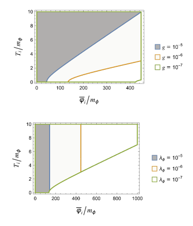
Figure 1: Initial conditions that fall within the perturbative regime with fixed masses $m_{\phi}=500{\rm GeV}$, $m_{\chi}=150{\rm GeV}$. $\lambda_{\phi}=10^{-6}$ for the upper panel and $g=10^{-6}$ for the lower panel.

4.1 “Freeze-out” of the condensate

Before we present the exact numerical results, let us first estimate the condition for the “freeze-out” of the condensate. From Eq. (15), one can read the condensate decay rate as

$$\Gamma_{\varphi}=2\gamma-\frac{\dot{M}_{\phi}}{M_{\phi}}+\frac{2\sigma\rho_{\varphi}}{M^{2}_{\phi}}\,.$$ (28)

In general, an efficient decay requires $\Gamma_{\varphi}\;\raisebox{-3.00003pt}{$\stackrel{{\scriptstyle\displaystyle>}}{{\sim}}$}\;H$ so that one can use $\Gamma_{\varphi}\sim H$ as an estimate of the “freeze-out” time of the condensate. The full evolution is complicated because there could be some reheating effects due to the energy transfer from the condensate to the plasma. However, the “freeze-out” of the condensate typically occurs after the reheating. At that stage, one would have $\rho_{\rm R}\gg\rho_{\varphi}$, and

$$H\sim 1.66\times\sqrt{g_{*}}T^{2}\sim\mathcal{O}(10)\,T^{2}\sim\frac{1}{t}\,.$$ (29)

$\gamma$ channels

In the high-temperature limit, $\gamma$ exhibits a decrease proportional to the temperature $T$ as the Universe cools down. When the temperature drops to the regime where $M_{\phi}\sim m_{\phi}$, $\gamma$ decreases with a quadratic dependence on $T$, thus scaling as $T^{2}$. At lower temperatures, $\gamma$ experiences an exponential suppression. As a consequence, when the temperature drops to a sufficiently low value, $\gamma$ decreases faster than $H$.

$\sigma$ channel

While $\sigma$ is not vanishing even for $T\rightarrow 0$ provided $m_{\phi}>m_{\chi}$, the condensate decay rate due to the sigma channel is proportional to $\rho_{\varphi}$ which decreases fast. For the case of $\gamma=0$ and $\dot{M}_{\phi}=0$, $\rho_{\varphi}$ drops as $t^{-3/2}$ [44] while $H$ drops as $1/t$. With nonvanishing $\gamma$ and $\dot{M}_{\phi}$, $\rho_{\varphi}$ should decrease even faster.

Damping due to the change of $M_{\phi}$

In the high-temperature limit, one has

$$-\frac{\dot{M}_{\phi}}{M_{\phi}}=\frac{(\lambda_{\phi}+g)T\dot{T}/24}{\sqrt{m^{2}_{\phi}+(\lambda_{\phi}+g)T^{2}/24}}\sim\sqrt{\frac{\lambda_{\phi}+g}{24}}\left(\frac{\dot{T}}{T}\right)$$ (30)

which scales as $H$ but with a suppressed factor $\sqrt{(\lambda_{\phi}+g)/24}$. Going beyond the high temperature limit, $-\dot{M_{\phi}}/M_{\phi}$ decreases faster and quickly approaches zero when $(\lambda_{\phi}+g)T^{2}/24<m_{\phi}^{2}$. Actually, in the parameter region for our numerical calculations, $-\dot{M}_{\phi}/M_{\phi}$ is negligible.

In summary, $\Gamma_{\varphi}$ would decrease faster than $H$ as the Universe cools down and therefore the condensate must “freeze out” at some point. This will be confirmed further with our numerical results below. We emphasize that it is crucial to go beyond the high-temperature approximation for $\gamma$. Otherwise, one can have, for some chosen parameters, a $\gamma$ that is larger than $H$ all the time and conclude that the condensate energy can be fully transferred to radiation [43, 44]. The above analysis does not draw any conclusion about the relic density of the condensate. The latter strongly depends on the parameters in the theory as well as the initial condition.

4.2 $m_{\phi}>m_{\chi}$

Let us first consider the case $m_{\phi}=500{\rm GeV}>m_{\chi}=150{\rm GeV}$.

Different couplings

We fix the initial condition as $\bar{\varphi}_{i}=5m_{\phi}$, $T_{i}=2m_{\phi}$ and consider three sets of couplings: $\{g=10^{-7},\lambda_{\phi}=10^{-6}\}$, $\{g=10^{-6},\lambda_{\phi}=10^{-6}\}$, and $\{g=10^{-6},\lambda_{\phi}=10^{-5}\}$. Fig. 2 shows the relic comoving energy density $\rho_{\varphi}a^{3}$ for these three cases while Fig. 3 shows the details about the evolution. For $g=10^{-7}$, $\lambda_{\phi}=10^{-6}$, the condensate decay is rather incomplete. This is because both $\gamma$ and $\sigma\rho_{\varphi}/M_{\phi}^{2}$ are smaller than $H$ all the time and no efficient decay can occur (see the first row of Fig. 3). For the second case, $\sigma\rho_{\varphi}/M_{\phi}^{2}$ is larger than $H$ initially while $\gamma$ is still smaller than $H$ all the time. Hence the decay is dominated by the $\sigma$ channel. However, due to dependence on $\bar{\varphi}^{2}$, $\sigma\rho_{\varphi}/M_{\phi}^{2}$ decreases quickly and the channel is efficient only for a short time, leading to again an incomplete decay. In the last case, $g=10^{-6}$, $\lambda_{\phi}=10^{-5}$, $\gamma$ is larger than $H$ for a period of the universe expansion and the decay is quite complete. In the last two cases, one clearly sees a “freeze-out” behavior of the condensate which is characterized by the crossing between the evolution line of either $\gamma$ or $\sigma\rho_{\varphi}/M_{\phi}^{2}$ and that of $H$. We note that even if the relic comoving energy density of the condensate is very small compared with the radiation comoving energy density, its actual relic energy density decreases slower than the radiation energy density and can catch up with the latter after a sufficiently long time of universe expansion. This should lead to additional phenomenological constraints on such $Z_{2}$-symmetric scalar fields. We leave a detailed study on this for future work.

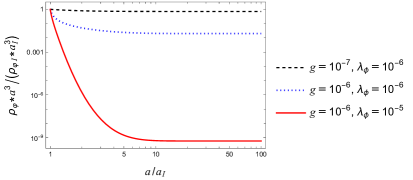
Figure 2: Relic comoving energy densities of the condensate with various coupling constants. The initial condition is chosen as $\bar{\varphi}_{i}=5m_{\phi}$, and $T_{i}=2m_{\phi}$.

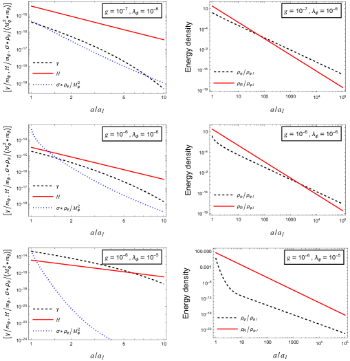
Figure 3: $\gamma$, $\sigma\rho_{\varphi}/M_{\phi}^{2}$ and the Hubble parameter $H$ (the first column) and the energy densities (the second column) for different couplings but with fixed initial condition $\bar{\varphi}_{i}=5m_{\phi}$, and $T_{i}=2m_{\phi}$.

Different initial conditions

Fig. 4 and Fig. 5 present the numerical solutions for different initial conditions, $\{\bar{\varphi}_{i}=m_{\phi},T_{i}=0.2m_{\phi}\}$, $\{\bar{\varphi}_{i}=5m_{\phi},T_{i}=0.2m_{\phi}\}$, and $\{\bar{\varphi}_{i}=m_{\phi},T_{i}=m_{\phi}\}$, but with fixed couplings $g=10^{-7}$, $\lambda_{\phi}=10^{-5}$. For the first initial condition, the decay is rather incomplete because both $\gamma$ and $\sigma\rho_{\varphi}/M_{\phi}^{2}$ are smaller than $H$ all the time. A larger value of either $\bar{\varphi}_{i}$ or $T_{i}$ can enhance the decay efficiency. A larger $\bar{\varphi}_{i}$ gives a larger initial decay rate of the $\sigma$ channel. Particle production from the $\sigma$ channel then leads to reheating and increases the temperature. As a consequence, the decay rate from the $\gamma$ channels increases at early times, see the left panel of the second row in Fig. 5. Increasing $T_{i}$ would directly increase $\gamma$ at the beginning, see the left panel of the third row in Fig. 5. Fig. 6 presents the evolution of $\gamma$, $\sigma\rho_{\varphi}/M_{\phi}^{2}$, and $H$ at early times for all the three cases.

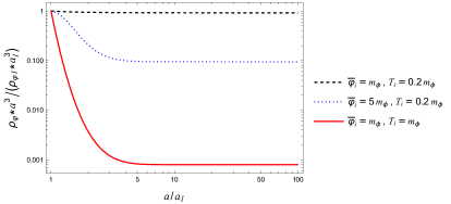
Figure 4: Comoving energy densities of the condensate for various initial conditions but with fixed couplings $g=10^{-7}$ and $\lambda_{\phi}=10^{-5}$.

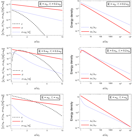
Figure 5: $\gamma$, $\sigma\rho_{\varphi}/M_{\phi}^{2}$ and the Hubble parameter $H$ (the first column) and the energy densities (the second column) for different initial conditions but fixed couplings $g=10^{-7}$ and $\lambda_{\phi}=10^{-5}$.

Figure 6: Early evolution of $\gamma$ and $\sigma\rho_{\varphi}/M_{\phi}^{2}$ with various initial conditions: $\{\bar{\varphi}_{i}=m_{\phi},T_{i}=0.2m_{\phi}\}$ (black), $\{\bar{\varphi}_{i}=5m_{\phi},T_{i}=0.2m_{\phi}\}$ (blue), $\{\bar{\varphi}_{i}=m_{\phi},T_{i}=m_{\phi}\}$ (red) with fixed couplings $g=10^{-7}$, $\lambda_{\phi}=10^{-5}$.

4.3 $m_{\phi}<m_{\chi}$

Now we consider the case $m_{\phi}=100{\rm GeV}<m_{\chi}=150{\rm GeV}$. In this case, one typically has $M_{\chi}>M_{\phi}$ unless $\lambda_{\phi}$ is too large which would then probably lead to unitarity problems. Therefore, for this case the $\sigma$ channel is closed.

Different couplings

Again we fix the initial condition to $\bar{\varphi}_{i}=5m_{\phi}$ and $T_{i}=2m_{\phi}$. Fig. 7 presents the obtained comoving energy densities of the condensate for $\{g=10^{-7},\lambda_{\phi}=10^{-6}\}$, $\{g=10^{-6},\lambda_{\phi}=10^{-6}\}$ and $\{g=10^{-7},\lambda_{\phi}=3*10^{-6}\}$. The “freeze-out” behavior can be explained by the evolution of $\gamma$ and $H$ shown in Fig. 8.

Figure 7: Comoving energy densities of the condensate for various coupling constants but with fixed initial condition $\bar{\varphi}_{i}=5m_{\phi}$, and $T_{i}=2m_{\phi}$.

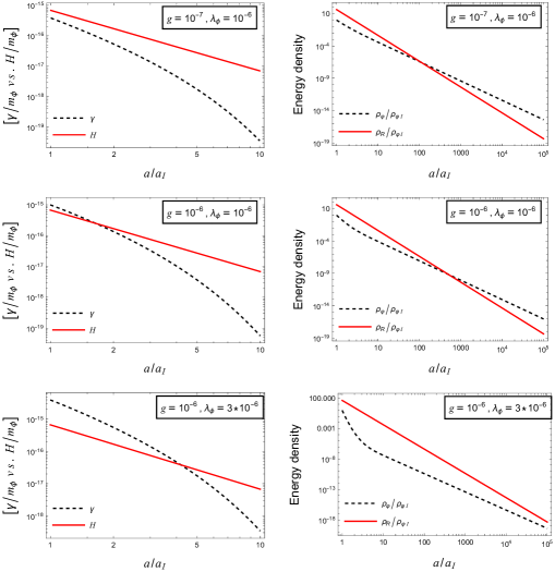
Figure 8: $\gamma$ and the Hubble parameter $H$ (the first column) and the energy densities (the second column) for different couplings but fixed initial condition $\bar{\varphi}_{i}=5m_{\phi}$, and $T_{i}=2m_{\phi}$.

Different initial conditions

Figs. 9 and 10 present the numerical solutions for different initial conditions, $\{\bar{\varphi}_{i}=m_{\phi},T_{i}=0.2m_{\phi}\}$, $\{\bar{\varphi}_{i}=5m_{\phi},T_{i}=0.2m_{\phi}\}$, and $\{\bar{\varphi}_{i}=m_{\phi},T_{i}=m_{\phi}\}$, but fixed couplings $g=10^{-6}$, $\lambda_{\phi}=10^{-5}$. Similar to the case $m_{\phi}>m_{\chi}$, a larger $T_{i}$ would directly increase $\gamma$ at the beginning, hence improving the decay efficiency. However, we still observe an enhancement of the decay rate with a larger initial oscillation amplitude even though the $\sigma$ channel is closed. This is again due to reheating effects from particle production but via the $\gamma$ channels now. In the middle panel of Fig. 10, one can see an early increase of $\gamma$ (reheating), which is followed by a slower decrease. The evolution of the temperature in three cases is shown in Fig. 11.

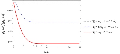
Figure 9: Comoving energy densities of the condensate for various initial conditions with fixed couplings $g=10^{-6}$ and $\lambda_{\phi}=10^{-5}$.

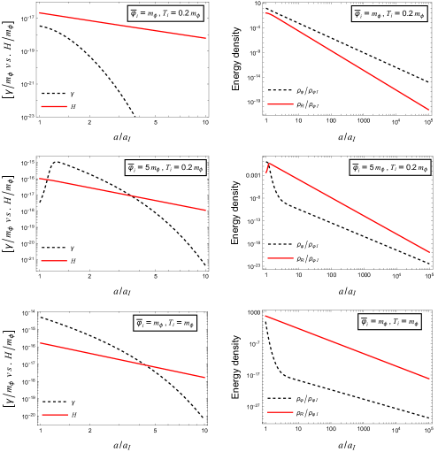
Figure 10: Numerical solutions for coupled equations (15), (16), and (17). The first column shows the evolution of $\gamma$ and the Hubble parameter $H$. The second column shows the evolution of energy densities.

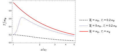
Figure 11: Evolution of radiation temperature for various initial conditions with fixed couplings $g=10^{-6}$ and $\lambda_{\phi}=10^{-5}$.

5 Conclusion and discussion

In this work, we have studied the evolution of homogeneous $Z_{2}$-symmetric scalar condensates in the early Universe in the perturbative regime where the oscillation amplitude is sufficiently small so that dissipation occurs via perturbative processes. This also indicates that the oscillation is quasi-harmonic. Otherwise, self-interactions of the scalar field would lead to significant parametric resonance. This perturbative regime necessarily comprises the late stage of the condensate evolution and determines the fate of the condensate. Our analysis is based on the CTP formalism which naturally accommodates quantum statistical effects of the plasma as well as the backreaction effects from particle production.

We have derived, in the perturbative regime, the coupled coarse-grained equations of motion for the condensate energy, radiation, and spacetime from the original non-local condensate equation of motion obtained from nonequilibrium quantum field theory. This derivation makes use of the multi-scale analysis that was first introduced in Ref. [36] to study the dissipation of scalar background fields. In this work, we have extended the analysis in Ref. [36] to take into account both the expanding spacetime and the time dependence in the temperature. The coarse-grained equations of motion depend on two microscopic quantities $\gamma$ and $\sigma$, defined in Eq. (2), which have an interpretation in terms of particle production. We have presented a very detailed computation of these two quantities. The analytic result for $\gamma$ contributed from the sunset diagram generated by the $\varphi\phi\chi^{2}$ interaction (the second diagram from Eq. (8a)) is a new result. The coupled equations of motion have been solved numerically.

The key finding in this work is that a scalar condensate with $Z_{2}$ symmetry cannot transfer all its energy to the plasma. The condensate decay rate is given in Eq. (28) and depends on both the temperature and the oscillation amplitude (through $\rho_{\varphi}$). As a result, the condensate decay rate always decreases faster than the Hubble parameter at late times (see the analysis in Sec. 4.1). Therefore, similar to the freeze-out process for particles, the condensate comoving energy density approaches a constant once the condensate decay rate drops below the Hubble parameter. A homogeneous $Z_{2}$-symmetric scalar condensate must have a nonvanishing relic density. This should put additional constraints on $Z_{2}$-symmetric scalar fields as dark matter.

In our model, we did not consider spontaneous symmetry breaking. If $m_{\chi}^{2}<0$, as it would be when $\chi$ is identified as the Higgs, there may be spontaneous symmetry breaking during the evolution of the condensate. If such spontaneous symmetry breaking occurs, we should have a cubic interaction term $v\Phi^{2}\chi$ where $v$ is the symmetry broken value of the $\chi$ field. In the presence of the condensate, one has the vertex $v\varphi\phi\chi$ which leads to the following additional diagram in the effective action that contributes to the condensate decay,

$$\leavevmode\leavevmode\hbox to80.17pt{\vbox to18.94pt{\text{[drawing]}}}\,.$$ (31)

This diagram would contribute to $\gamma$ because it induces a linear term in the equation of motion of $\varphi$. By the cutting rules [57, 58, 59, 60, 61, 62, 63], this diagram describes the scattering process $\varphi\phi\leftrightarrow\chi$ [the other processes ($\varphi\leftrightarrow\phi\chi$, $\varphi\chi\leftrightarrow\phi$) cannot satisfy the on-shell condition]. The process $\varphi\phi\leftrightarrow\chi$ again belongs to Landau damping and is suppressed at low temperatures. Therefore, $\gamma$ would still drop below $H$ at later times. The key finding discussed above is thus not affected by a spontaneous symmetry breaking from the $\chi$ field but the actual evolution of the condensate may be quite different.

Appendix A Closed-Time-Path formalism

In this section, we give a brief introduction to the CTP formalism, with the main purpose of setting up the notation. For a more detailed introduction, we refer to Refs. [70, 71, 72]. The CTP formalism has been widely applied to the studies of baryogenesis, especially in the form of leptogenesis (see, e.g., Refs. [74, 75, 76, 77, 78, 79, 80, 81, 82, 83, 84, 85, 86, 87, 88]).

Out-of-equilibrium dynamics is an initial-value problem with the initial conditions given by a density matrix at a given time, $\rho_{D}(t_{i})$. The expectation value of an observable $\mathcal{O}$ at time $t$ is given by

$$\langle\mathcal{O}(t)\rangle={\rm Tr}\left\{\rho_{D}(t_{i})\mathcal{O}(t)\right\}\,,$$ (A32)

where $\mathcal{O}(t)=\exp(\mathrm{i}H(t-t_{i}))\mathcal{O}(t_{i})\exp(-\mathrm{i}H(t-t_{i}))$. The operator is sandwiched between the same state. For this reason, the CTP formalism is also called in-in formalism. Viewed from the Schrödinger picture, the state evolves first forward in time from $t_{i}$ to $t$ and then backward in time to $t_{i}$. Expectation values can thus be obtained by a generating functional formulated on a closed time contour $\mathcal{C}$, as illustrated in Fig. 12. For the quantity given in Eq. (A32), $t_{f}=t$, but one can also choose any $t_{f}\geq t$ by inserting an operator $\exp(\mathrm{i}H(t-t_{f}))\exp(-\mathrm{i}H(t_{f}-t))=\mathbf{1}$ on the left of $\mathcal{O}(t)$ in Eq. (A32). In particular, one can choose $t_{f}\rightarrow\infty$ so that the generating functional is independent of the quantities to be computed.

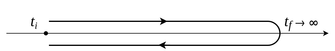
Figure 12: The Keldysh contour $\mathcal{C}$ for the generating functional in the CTP formalism. In the plot, the forward and backward time contours are slightly shifted off the real line only for the purpose of illustration; both contours should be understood as lying exactly on the real line.

All the information in a quantum field system is encoded in its correlation functions. For most purposes, it is sufficient to study the one- and two-point functions. For the scalar field $\Phi$, there are two independent connected two-point functions

$$\langle\Phi(x_{1})\Phi(x_{2})\rangle_{c} =\langle\phi(x_{1})\phi(x_{2})\rangle\equiv\Delta_{\phi}^{>}(x_{1},x_{2})\,,$$ (A33a)

$$\langle\Phi(x_{2})\Phi(x_{1})\rangle_{c} =\langle\phi(x_{2})\phi(x_{1})\rangle\equiv\Delta_{\phi}^{<}(x_{1},x_{2})\,.$$ (A33b)

Here and in what follows, analogous expressions also apply for the $\chi$ field and corresponding quantities are denoted similarly with the subscript $\phi$ replaced by $\chi$. Since the generating functional is formulated on the closed time contour $\mathcal{C}$, we would have two-point functions time-ordered on $\mathcal{C}$,

$$\Delta^{\mathcal{C}}_{\phi}(x_{1},x_{2})=\theta_{\mathcal{C}}(t_{1},t_{2})\Delta_{\phi}^{>}(x_{1},x_{2})+\theta_{\mathcal{C}}(t_{2},t_{1})\Delta_{\phi}^{<}(x_{1},x_{2})\,.$$ (A34)

To distinguish the times on the forward and backward contours in $\Delta^{\mathcal{C}}_{\phi}$, one can denote the forward time with a superscript “$+$” and the backward time “$-$”: $x^{+}=\{t^{+},\mathbf{x}\}$, $x^{-}=\{t^{-},\mathbf{x}\}$. According to the $\mathcal{C}$-ordering, one would have

$$\Delta^{\mathcal{C}}_{\phi}(x_{1}^{+},x_{2}^{-}) =\Delta_{\phi}^{<}(x_{1},x_{2})\,,$$ (A35a)

$$\Delta^{\mathcal{C}}_{\phi}(x_{1}^{-},x_{2}^{+}) =\Delta_{\phi}^{>}(x_{1},x_{2})\,,$$ (A35b)

$$\Delta^{\mathcal{C}}_{\phi}(x_{1}^{+},x_{2}^{+}) =\langle T\phi(x_{1})\phi(x_{2})\rangle\,,$$ (A35c)

$$\Delta^{\mathcal{C}}_{\phi}(x_{1}^{-},x_{2}^{-}) =\langle\overline{T}\phi(x_{1})\phi(x_{2})\rangle\,,$$ (A35d)

where $T$ and $\overline{T}$ denote the normal time-ordering and anti-time-ordering operators, respectively.

Compared to the closed time variable, a more convenient notation is the “double-field” formulation where one distinguishes the fields on the forward contour from those on the backward contour while using a common time variable. For example, one denotes $\Phi(x^{+})$ as $\Phi^{+}(x)$, $\Phi(x^{-})$ as $\Phi^{-}(x)$, and similarly for $\chi$. Then the action integrated over the contour $\mathcal{C}$ can be written as

$$S_{\mathcal{C}}[\Phi,\chi]=S[\Phi^{+},\chi^{+}]-S[\Phi^{-},\chi^{-}]\,,$$ (A36)

where the minus sign is due to the backward direction in the integral on the backward contour in $S_{\mathcal{C}}[\Phi,\chi]$. In this notation, Eq. (A35) can be rewritten as

$$\Delta^{+-}_{\phi}(x_{1},x_{2}) =\Delta_{\phi}^{<}(x_{1},x_{2})\,,$$ (A37a)

$$\Delta^{-+}_{\phi}(x_{1},x_{2}) =\Delta_{\phi}^{>}(x_{1},x_{2})\,,$$ (A37b)

$$\Delta^{++}_{\phi}(x_{1},x_{2}) =\langle T\phi(x_{1})\phi(x_{2})\rangle\,,$$ (A37c)

$$\Delta^{--}_{\phi}(x_{1},x_{2}) =\langle\overline{T}\phi(x_{1})\phi(x_{2})\rangle\,.$$ (A37d)

The indices “$\pm$” are called the Schwinger-Keldysh polarity indices.

Usually, it is convenient to introduce the spectral and statistical correlation functions defined as, respectively,

$$\Delta_{\phi}^{-}(x_{1},x_{2}) =\mathrm{i}\langle[\Phi(x_{1}),\Phi(x_{2})]\rangle_{c}=\mathrm{i}\left(\Delta_{\phi}^{-+}(x_{1},x_{2})-\Delta_{\phi}^{+-}(x_{1},x_{2})\right)\,,$$ (A38a)

$$\Delta_{\phi}^{+}(x_{1},x_{2}) =\frac{1}{2}\langle\{\Phi(x_{1}),\Phi(x_{2})\}\rangle_{c}=\frac{1}{2}\left(\Delta_{\phi}^{-+}(x_{1},x_{2})+\Delta_{\phi}^{+-}(x_{1},x_{2})\right)\,.$$ (A38b)

The spectral correlation function encodes the information about the spectrum of the theory and the statistical correlation function gives the information about occupation numbers of different modes for the fluctuations.

The Schwinger-Dyson equations for the one- and two-point functions can be derived from the one-particle-irreducible (1PI) or two-particle-irreducible (2PI) effective actions [55, 56]. Here we use the 2PI effective action. If the effective action is not truncated, the 1PI and 2PI give the same equations of motion. For a given order in the loop expansion, the 2PI effective action includes resummation in the propagators compared to the 1PI effective action. The definition of the 2PI effective action is based on the generating functional with local and non-local sources,

$$Z[J_{\Phi},J_{\chi},K_{\Phi},K_{\chi}]=\int\mathcal{D}\Phi^{+}\mathcal{D}\Phi^{-}\mathcal{D}\chi^{+}\mathcal{D}\chi^{-}\,$$

$$\times\exp\left(\mathrm{i}\left[S[\Phi^{+},\chi^{+}]-S[\Phi^{-},\chi^{-}]+J^{A}_{\Phi,x}\Phi^{A}_{x}+J^{A}_{\chi,x}\chi^{A}_{x}+\frac{1}{2}\Phi^{A}_{x}K^{AB}_{\Phi,xy}\Phi^{B}_{y}+\frac{1}{2}\chi^{A}_{x}K^{AB}_{\chi,xy}\chi^{B}_{y}\right]\right).$$ (A39)

where $A,B=\pm$, and we have used the DeWitt notation

$$J^{A}_{\Phi,x}\Phi^{A}_{x}=\int\mathrm{d}^{4}x\,J^{A}_{\Phi}(x)\Phi^{A}(x)\,,$$ (A40a)

$$\Phi^{A}_{x}K^{AB}_{\Phi,xy}\Phi^{B}_{y}=\int\mathrm{d}^{4}x\,\mathrm{d}^{4}y\,\Phi^{A}(x)K^{AB}_{\Phi}(x,y)\Phi^{B}(y)\,.$$ (A40b)

The Einstein summation convention is understood for repeated indices. One can easily check that

$$\frac{\delta\ln Z[J_{\Phi},J_{\chi},K_{\Phi},K_{\chi}]}{\mathrm{i}\delta J^{A}_{\Phi}(x)} =\langle\Phi^{A}(x)\rangle\equiv\varphi^{A}(x)\,,$$ (A41a)

$$\frac{\delta\ln Z[J_{\Phi},J_{\chi},K_{\Phi},K_{\chi}]}{\mathrm{i}\delta K^{AB}_{\Phi,xy}} =\frac{1}{2}\left(\Delta^{AB}_{\phi}(x_{1},x_{2})+\varphi^{A}(x)\varphi^{B}(y)\right)\,,$$ (A41b)

and similarly for quantities involving $\chi$. Note that in the above equations, the one- and two-point functions on the RHS are defined with corresponding sources. The 2PI effective action is then defined as the Legendre transform,

$$\Gamma_{\rm 2PI}[\varphi,\bar{\chi},\Delta_{\phi},\Delta_{\chi}]= -\mathrm{i}\,\ln Z[J_{\Phi},J_{\chi},K_{\Phi},K_{\chi}]-J^{A}_{\Phi,x}\varphi^{A}_{x}-J^{A}_{\chi,x}\bar{\chi}^{A}_{x}\,,$$ (A42)

$$-\frac{1}{2}K^{AB}_{\Phi,xy}(\varphi^{A}_{x}\varphi^{B}_{y}+\Delta^{AB}_{\phi,xy})-\frac{1}{2}K^{AB}_{\chi,xy}(\bar{\chi}_{x}^{A}\bar{\chi}_{y}^{B}+\Delta_{\chi,xy}^{AB})\,,$$ (A43)

where $\bar{\chi}^{A}=\langle\chi^{A}\rangle$. The Schwinger-Dyson equations for the one- and two-point functions read

$$\frac{\delta\Gamma_{\rm 2PI}[\varphi,\bar{\chi},\Delta_{\phi},\Delta_{\chi}]}{\delta\varphi^{A}(x)}=-J^{A}_{\Phi}(x)-K^{AB}_{\Phi,xy}\varphi^{B}_{y}\,,$$ (A44a)

$$\frac{\delta\Gamma_{\rm 2PI}[\varphi,\bar{\chi},\Delta_{\phi},\Delta_{\chi}]}{\delta\Delta^{AB}_{\phi/\chi}(x,y)}=-\frac{1}{2}K^{AB}_{\Phi/\chi}(x,y)\,.$$ (A44b)

Taking all the $J$ and $K$ to be vanishing, we obtain the equations of motion in the absence of external sources

$$\left.\frac{\delta\Gamma_{\rm 2PI}[\varphi,\bar{\chi},\Delta_{\phi},\Delta_{\chi}]}{\delta\varphi^{+}(x)}\right|_{\varphi^{-}=\varphi^{+}=\varphi}=0\,,$$ (A45)

$$\quad\left.\frac{\delta\Gamma_{\rm 2PI}[\varphi,\bar{\chi},\Delta_{\phi},\Delta_{\chi}]}{\delta\Delta^{AB}_{\phi/\chi}(x,y)}\right|_{\varphi^{-}=\varphi^{+}=\varphi}=0\,.$$ (A46)

In the Feynman-diagram representation of the $2$PI effective action, we now have two types of vertices: the + and - types. Depending on the vertices, one would have four different types of propagators: $\Delta_{\phi/\chi}^{++}$, $\Delta_{\phi/\chi}^{+-}$, $\Delta_{\phi/\chi}^{-+}$, and $\Delta_{\phi/\chi}^{--}$. For example, a propagator connecting two + type vertices is of type $\Delta^{++}$, etc. Solving first on-shell for the two-point functions and assuming that $\bar{\chi}=0$, one gets $\Delta_{\phi}[\varphi]$ and $\Delta_{\chi}[\varphi]$ as functionals of the condensate $\varphi$. Plugging them back into the 2PI effective action gives the EoM for the condensate

$$\left.\frac{\delta\Gamma_{\text{2PI}}[\varphi,\Delta_{\phi},\Delta_{\chi}]}{\delta\varphi(x)}\right|_{\Delta_{\phi}=\Delta_{\phi}[\varphi],\,\Delta_{\chi}=\Delta_{\chi}[\varphi]}=0\,.$$ (A47)

Arriving here, one can follow Section 2 of Ref. [36] to perform the small-field expansion of the on-shell two-point functions $\Delta_{\phi}[\varphi]$ and $\Delta_{\chi}[\varphi]$. To the lowest order, they are independent of $\varphi$ and become the free thermal equilibrium propagators. Properly truncating the effective action, one ends up with Eq. (7).

Appendix B Self-energies

The Feynman-diagram rules for the free thermal equilibrium propagators with thermal corrections to the masses taken into account are

$$\leavevmode\leavevmode\hbox to59.87pt{\vbox to15.57pt{\text{[drawing]}}}\equiv G_{\phi}^{AB}(x-x^{\prime})\,,\qquad\qquad\leavevmode\leavevmode\hbox to59.87pt{\vbox to15.57pt{\text{[drawing]}}}\equiv G_{\chi}^{AB}(x-x^{\prime})\,, \scriptstyle(x,A) \scriptstyle(x^{\prime},B) \scriptstyle(x,A) \scriptstyle(x^{\prime},B) \scriptstyle(x,A) \scriptstyle(x^{\prime},B) \scriptstyle(x,A) \scriptstyle(x^{\prime},B)$$ (B48)

where

$$G_{\phi/\chi}^{++}(x-x^{\prime})= \int\frac{\mathrm{d}^{4}k}{(2\pi)^{4}}\,\mathrm{e}^{-\mathrm{i}k(x-x^{\prime})}\left[\frac{\mathrm{i}}{k^{2}-M_{\phi/\chi}^{2}+\mathrm{i}\varepsilon}+2\pi f_{\rm B}(|k_{0}|)\delta\left(k^{2}-M_{\phi/\chi}^{2}\right)\right]\,,$$ (B49a)

$$G_{\phi/\chi}^{+-}(x-x^{\prime})= \int\frac{\mathrm{d}^{4}k}{(2\pi)^{4}}\,\mathrm{e}^{-\mathrm{i}k(x-x^{\prime})}\left[2\pi f_{\rm B}(k_{0})\rm sign(k_{0})\,\delta\left(k^{2}-M_{\phi/\chi}^{2}\right)\right]\,,$$ (B49b)

with the remaining components being complex conjugates, $G^{--}_{\phi/\chi}(x-x^{\prime})=\left[G^{++}_{\phi/\chi}(x-x^{\prime})\right]^{*}$, $G^{-+}_{\phi/\chi}(x-x^{\prime})=\left[G^{+-}_{\phi/\chi}(x-x^{\prime})\right]^{*}$. Here, the thermally corrected masses are

$$M_{\phi}^{2} =m_{\phi}^{2}-\frac{\mathrm{i}\lambda_{\phi}}{2}\leavevmode\leavevmode\hbox to52.4pt{\vbox to28.95pt{\text{[drawing]}}}-\frac{\mathrm{i}g}{2}\leavevmode\leavevmode\hbox to52.4pt{\vbox to28.95pt{\text{[drawing]}}}\,, \scriptstyle(x,+) \scriptstyle(x,+) \scriptstyle(x,+) \scriptstyle(x,+)$$ (B50a)

$$M_{\chi}^{2} =m_{\chi}^{2}-\frac{\mathrm{i}\lambda_{\chi}}{2}\leavevmode\leavevmode\hbox to52.4pt{\vbox to28.95pt{\text{[drawing]}}}-\frac{\mathrm{i}g}{2}\leavevmode\leavevmode\hbox to52.4pt{\vbox to28.95pt{\text{[drawing]}}}+({\rm other\ diagrams\ with\ SM\ fields})\,. \scriptstyle(x,+) \scriptstyle(x,+) \scriptstyle(x,+) \scriptstyle(x,+)$$ (B50b)

In the high-temperature approximation, we have

$$M^{2}_{\phi} =m_{\phi}^{2}+(\lambda_{\phi}+g)\frac{T^{2}}{24}\,,$$ (B51a)

$$M_{\chi}^{2} =m_{\chi}^{2}+(\lambda_{\chi}+g)\frac{T^{2}}{24}+\kappa^{2}T^{2}\,,$$ (B51b)

where $\kappa^{2}T^{2}$ is due to possible interactions between $\chi$ and the SM fields. We shall take $\kappa^{2}\approx 0.1$ in our numerical calculations, which corresponds to roughly the value of the thermal corrections to the Higgs mass in the SM.

The various self-energies and proper four-vertex functions read

$$\Pi^{AB}(x-x^{\prime}) =\ -\,\frac{\mathrm{i}(AB)\lambda_{\phi}^{2}}{6}\,\leavevmode\leavevmode\hbox to80.31pt{\vbox to28.95pt{\text{[drawing]}}}\ -\ \frac{\mathrm{i}(AB)g^{2}}{2}\,\leavevmode\leavevmode\hbox to80.31pt{\vbox to28.95pt{\text{[drawing]}}}\,, \scriptstyle(x,A) \scriptstyle(x^{\prime},B) \scriptstyle(x^{\prime},B) \scriptstyle(x,A) \scriptstyle(x,A) \scriptstyle(x^{\prime},B) \scriptstyle(x^{\prime},B) \scriptstyle(x,A)$$ (B52a)

$$V^{AB}(x-x^{\prime}) =\ -\ \frac{3\mathrm{i}(AB)\lambda_{\phi}^{2}}{2}\,\leavevmode\leavevmode\hbox to80.31pt{\vbox to28.95pt{\text{[drawing]}}}\ -\ \frac{3\mathrm{i}(AB)g^{2}}{2}\,\leavevmode\leavevmode\hbox to78.64pt{\vbox to28.95pt{\text{[drawing]}}}\,. \scriptstyle(x^{\prime},B) \scriptstyle(x,A) \scriptstyle(x^{\prime}\!,B) \scriptstyle(x,A) \scriptstyle(x^{\prime},B) \scriptstyle(x,A) \scriptstyle(x^{\prime}\!,B) \scriptstyle(x,A)$$ (B52b)

The retarded self-energy and retarded proper four-vertex function are then defined as

$$\Pi^{\rm R}(x-x^{\prime})=\Pi^{++}(x-x^{\prime})+\Pi^{+-}(x-x^{\prime})=\theta(t-t^{\prime})\left[-\Pi^{-+}(x-x^{\prime})+\Pi^{+-}(x-x^{\prime})\right]\,,$$ (B53a)

$$V^{\rm R}(x-x^{\prime})=V^{++}(x-x^{\prime})+V^{+-}(x-x^{\prime})=\theta(t-t^{\prime})\left[-V^{-+}(x-x^{\prime})+V^{+-}(x-x^{\prime})\right]\,.$$ (B53b)

And $\pi^{\rm R}$ and $v^{\rm R}$ are defined as

$$\pi^{\rm R}(t-t^{\prime})=\int\mathrm{d}^{3}x\,\Pi^{\rm R}(x-x^{\prime})\,,\qquad v^{\rm R}(t-t^{\prime})=\int\mathrm{d}^{3}x\,V^{\rm R}(x-x^{\prime})\,.$$ (B54)

Important quantities that would appear in the solutions for the condensate evolution are Fourier transforms of the retarded self-energy and proper four-vertex function, which are defined as

$$\widetilde{\pi}^{\rm R}(\omega)=\int_{-\infty}^{\infty}\,\mathrm{d}t^{\prime}\,\mathrm{e}^{\mathrm{i}\omega(t-t^{\prime})}\,\pi^{\rm R}(t-t^{\prime})\,,\qquad\quad\widetilde{v}^{\rm R}(\omega)=\int_{-\infty}^{\infty}\,\mathrm{d}t^{\prime}\,\mathrm{e}^{\mathrm{i}\omega(t-t^{\prime})}\,v^{\rm R}(t-t^{\prime})\,.$$ (B55)

Note that

$$\widetilde{\pi}^{\rm R}(\omega)=\widetilde{\Pi}^{\rm R}(\omega,\mathbf{p}=0)\,,\qquad\quad\widetilde{v}^{\rm R}(\omega)=\widetilde{V}^{\rm R}(\omega,\mathbf{p}=0)\,,$$ (B56)

where $\omega=p_{0}$ and $\widetilde{\Pi}^{\rm R}$ and $\widetilde{V}^{\rm R}$ are Fourier transforms of $\Pi^{\rm R}$ and $V^{\rm R}$, respectively.

In terms of the free thermal propagators, the retarded self-energy and proper four-vertex function in position space read

$$\Pi^{\rm R}(x-x^{\prime})\equiv \Pi_{\phi}^{\rm R}(x-x^{\prime})+\Pi_{\chi}^{\rm R}(x-x^{\prime})=-\frac{\mathrm{i}\lambda_{\phi}^{2}}{6}\left[\left(G^{++}_{\phi}(x-x^{\prime})\right)^{3}-\left(G_{\phi}^{+-}(x-x^{\prime})\right)^{3}\right]$$

$$\quad-\frac{\mathrm{i}g^{2}}{2}\left[\left(G_{\chi}^{++}(x-x^{\prime})\right)^{2}G_{\phi}^{++}(x-x^{\prime})-\left(G_{\chi}^{+-}(x-x^{\prime})\right)^{2}G_{\phi}^{+-}(x-x^{\prime})\right]\,,$$ (B57a)

$$V^{\rm R}(x-x^{\prime})\equiv V_{\phi}^{\rm R}(x-x^{\prime})+V_{\chi}^{\rm R}(x-x^{\prime})=-\frac{3\mathrm{i}\lambda_{\phi}^{2}}{2}\left[\left(G_{\phi}^{++}(x-x^{\prime})\right)^{2}-\left(G_{\phi}^{+-}(x-x^{\prime})\right)^{2}\right]$$

$$\quad-\frac{3\mathrm{i}g^{2}}{2}\left[\left(G_{\chi}^{++}(x-x^{\prime})\right)^{2}-\left(G_{\chi}^{+-}(x-x^{\prime})\right)^{2}\right]\,.$$ (B57b)

B.1 Proper four-vertex function

As a warm-up, in this subsection we present the calculation of ${\rm Im}\widetilde{V}^{\rm R}(p)$ which gives $\sigma$ when evaluated at $p=(2M_{\phi},\mathbf{0})$. In the next subsection, we will present the more complicated calculation for $\gamma$.

B.1.1 Summary of the results

Let us first introduce a quantity $V^{-}$ that in position space reads

$$V^{-}(x-x^{\prime})\equiv V_{\phi}^{-}(x-x^{\prime})+V_{\chi}^{-}(x-x^{\prime}) =\sum_{a=\phi,\chi}c_{a}\left[\left(G^{-+}_{a}(x-x^{\prime})\right)^{2}-\left(G^{+-}_{a}(x-x^{\prime})\right)^{2}\right]$$

$$=-2\mathrm{i}\sum_{a=\phi,\chi}c_{a}G_{a}^{+}(x-x^{\prime})G_{a}^{-}(x-x^{\prime})\,,$$ (B58)

where $c_{\phi}=-3\mathrm{i}\lambda_{\phi}^{2}/2$, $c_{\chi}=-3\mathrm{i}g^{2}/2$. The imaginary part of the retarded proper four-vertex function in momentum space, ${\rm Im}\widetilde{V}^{\rm R}(p)$, is related to $\widetilde{V}^{-}(p)$ through (see, e.g., Ref. [94])

$${\rm Im}\widetilde{V}^{\rm R}(p)=-\frac{\mathrm{i}}{2}\widetilde{V}^{-}(p)\,,$$ (B59)

where $\widetilde{V}^{-}(p)$ is the Fourier transform of $V^{-}(x-x^{\prime})$,

$$\widetilde{V}^{-}(p)=\sum_{a=\phi,\chi}\widetilde{V}^{-}_{a}(p)=-2\mathrm{i}\sum_{a=\phi,\chi}c_{a}\int\frac{\mathrm{d}^{4}k}{(2\pi)^{4}}\left(G^{+}_{a}(k)G^{-}_{a}(p-k)\right)\,.$$ (B60)

The real part, ${\rm Re}\widetilde{V}^{\rm R}(p)$, is related to the imaginary part via the Kramers-Kronig relation

$${\rm Re}\widetilde{V}^{\rm R}(p)=\mathcal{P}\int\frac{\mathrm{d}\omega^{\prime}}{\pi}\frac{{\rm Im}\widetilde{V}^{\rm R}(\omega^{\prime},\mathbf{p})}{\omega^{\prime}-p_{0}}\,.$$ (B61)

Substituting the Kubo-Martin-Schwinger (KMS) relation

$$G_{a}^{+}(q)=-\mathrm{i}\left(\frac{1}{2}+f_{\rm B}(q_{0})\right)G_{a}^{-}(q)$$ (B62)

into Eq. (B60) and using the definition for the spectral function, $G^{-}_{a}(k)=\mathrm{i}\rho_{a,\mathbf{k}}(k_{0})$, one gets

$$\widetilde{V}^{-}_{a}(p) =c_{a}\int\frac{\mathrm{d}^{4}k_{1}}{(2\pi)^{4}}\frac{\mathrm{d}^{4}k_{2}}{(2\pi)^{4}}(2\pi)^{4}\delta^{(4)}(p-k_{1}-k_{2})[1+f_{\rm B}(k_{1,0})+f_{\rm B}(k_{2,0})]\rho_{a,\mathbf{k}_{1}}(k_{0})\rho_{a,\mathbf{k}_{2}}(k_{2,0})$$

$$\equiv c_{a}I_{a}(p)\,,$$ (B63)

where we have defined the integral $I_{a}(p)$. Using Eq. (B59), one finally arrives at

$${\rm Im}\widetilde{V}^{R}_{a}(p)\equiv-\frac{\mathrm{i}c_{a}}{2}I_{a}(p)\,.$$ (B64)

Substituting into the integral $I_{a}(p)$ the free thermal spectral function

$$\rho_{a,\mathbf{k}}(k_{0})=2\pi{\rm sign}(k_{0})\delta(k_{0}^{2}-\omega_{a,\mathbf{k}}^{2})\,,$$ (B65)

where $\omega^{2}_{a,\mathbf{k}}=M_{a}^{2}+\mathbf{k}^{2}$, one obtains (see below for the detailed derivation)

$$I_{a}(p) =\frac{\theta(p^{2}-4M_{a}^{2})}{8\pi|\mathbf{p}|}\left[\left(\Omega_{a,-}-\Omega_{a,+}\right)+2T\log\left(\frac{f_{\rm B}(\Omega_{a,-})}{f_{\rm B}(\Omega_{a,+})}\right)\right]$$

$$\qquad\qquad\qquad\qquad\qquad+\frac{\theta(-p^{2})}{8\pi|\mathbf{p}|}\left[-2\Omega_{a,+}+2T\log\left|\frac{f_{\rm B}(\Omega_{a,-})}{f_{\rm B}(\Omega_{a,+})}\right|\right]\,,$$ (B66)

where

$$\Omega_{a,\pm}=\frac{p_{0}}{2}\pm\frac{|{\mathbf{p}}|}{2}\sqrt{1-\frac{(2M_{a})^{2}}{p^{2}}}\,.$$ (B67)

Taking $\mathbf{p}\to\mathbf{0}$, one obtains

$$I_{a}(p_{0},\mathbf{0})=\frac{1}{8\pi}\sqrt{1-\frac{4M_{a}^{2}}{p_{0}^{2}}}\theta\left(p_{0}^{2}-4M_{a}^{2}\right)\left(1+2f_{\rm B}\left(\frac{p_{0}}{2}\right)\right)\,.$$ (B68)

Therefore

$${\rm Im}\widetilde{v}_{a}^{\rm R}(p_{0})={\rm Im}\widetilde{V}^{\rm R}_{a}(p_{0},\mathbf{0})=-\frac{\mathrm{i}c_{a}}{16\pi}\sqrt{1-\frac{4M_{a}^{2}}{p_{0}^{2}}}\theta\left(p_{0}^{2}-4M_{a}^{2}\right)\left(1+2f_{\rm B}\left(\frac{p_{0}}{2}\right)\right)\,.$$ (B69)

Taking further $p_{0}=2M_{\phi}$ and substituting the above into the definition of $\sigma$, one obtains Eq. (21).

B.1.2 Computation of $I_{a}$

Below for clarity we suppress the subscript “a”. Doing the integral over $k_{1,0}$ and $k_{2,0}$ and using

$$\delta(f(x))=\sum_{\rm roots}\frac{\delta(x-x_{i})}{|f^{\prime}(x_{i})|}\,,$$ (B70)

we obtain

$$I(p)=\int\frac{\mathrm{d}^{3}\mathbf{k}_{1}}{(2\pi)^{3}}\int\frac{\mathrm{d}^{3}\mathbf{k}_{2}}{(2\pi)^{3}}\frac{(2\pi)^{4}\delta^{(3)}(\mathbf{p}-\mathbf{k}_{1}-\mathbf{k}_{2})}{4\omega_{\mathbf{k}_{1}}\omega_{\mathbf{k}_{2}}}\mathcal{G}(p_{0},\omega_{\mathbf{k}_{1}},\omega_{\mathbf{k}_{2}})\,,$$ (B71)

where

$$\mathcal{G}(p_{0},\omega_{\mathbf{k}_{1}},\omega_{\mathbf{k}_{2}})=\sum_{\alpha_{1},\alpha_{2}=\pm}(\alpha_{1}\alpha_{2})\delta(p_{0}-\alpha_{1}\omega_{\mathbf{k}_{1}}-\alpha_{2}\omega_{\mathbf{k}_{2}})\left[1+f_{\rm B}(\alpha_{1}\omega_{\mathbf{k}_{1}})+f_{\rm B}(\alpha_{2}\omega_{\mathbf{k}_{2}})\right]\,.$$ (B72)

Now using the property

$$f_{\rm B}(-\omega_{\mathbf{k}})=-1-f_{\rm B}(\omega_{\mathbf{k}})\,,$$ (B73)

one can rewrite $\mathcal{G}$ as

$$\mathcal{G}(p_{0},\omega_{\mathbf{k}_{1}},\omega_{\mathbf{k}_{2}}) =\delta(p_{0}-\omega_{\mathbf{k}_{1}}-\omega_{\mathbf{k}_{2}})\left\{\left[1+f_{\rm B}(\omega_{\mathbf{k}_{1}})\right]\left[1+f_{\rm B}(\omega_{\mathbf{k}_{2}})\right]-f_{\rm B}(\omega_{\mathbf{k}_{1}})f_{\rm B}(\omega_{\mathbf{k}_{2}})\right\}$$

$$+\delta(p_{0}+\omega_{\mathbf{k}_{1}}+\omega_{\mathbf{k}_{2}})\left\{f_{\rm B}(\omega_{\mathbf{k}_{1}})f_{\rm B}(\omega_{\mathbf{k}_{2}})-\left[1+f_{\rm B}(\omega_{\mathbf{k}_{1}})\right]\left[1+f_{\rm B}(\omega_{\mathbf{k}_{2}})\right]\right\}$$

$$+\delta(p_{0}+\omega_{\mathbf{k}_{1}}-\omega_{\mathbf{k}_{2}})\left\{f_{\rm B}(\omega_{\mathbf{k}_{1}})\left[1+f_{\rm B}(\omega_{\mathbf{k}_{2}})\right]-\left[1+f_{\rm B}(\omega_{\mathbf{k}_{1}})\right]f_{\rm B}(\omega_{\mathbf{k}_{2}})\right\}$$

$$+\delta(p_{0}-\omega_{\mathbf{k}_{1}}+\omega_{\mathbf{k}_{2}})\left\{\left[1+f_{\rm B}(\omega_{\mathbf{k}_{1}})\right]f_{\rm B}(\omega_{\mathbf{k}_{2}})-f_{\rm B}(\omega_{\mathbf{k}_{1}})\left[1+f_{\rm B}(\omega_{\mathbf{k}_{2}})\right]\right\}\,.$$ (B74)

It is easy to see the antisymmetry $p_{0}\leftrightarrow-p_{0}$ in $\mathcal{G}$ and also in the integral $I(p)$, $I(p_{0},\mathbf{p})=-I(-p_{0},\mathbf{p})$. Without loss of generality, in the following calculations we take $p_{0}>0$.

Equation (B.1.2) has a very clear interpretation in terms of microscopic particles processes. Assuming that we consider $I_{\phi}(p)$ and $p_{0}>0$, the first line then describes the process $(\varphi\varphi)\leftrightarrow\phi_{1}\phi_{2}$ where $(\varphi\varphi)$ are the external condensate di-quanta while $\phi_{1}$, $\phi_{2}$ are two particles for the fluctuation field $\phi$. Parent particles or daughter particles can be distinguished by the factors from the Boltzmann distributions multiplied with the $\delta$-functions. For example, the factor $1+f_{\rm B}(\omega_{\mathbf{k}_{1}})$ indicates that the particle $\phi_{1}$ is a daughter particle while $f_{\rm B}(\omega_{\mathbf{k}_{1}})$ indicates that $\phi_{1}$ is a parent particle. Therefore, when multiplied with $\left[1+f_{\rm B}(\omega_{\mathbf{k}_{1}})\right]\left[1+f_{\rm B}(\omega_{\mathbf{k}_{2}})\right]$, the first $\delta$-function describes $(\varphi\varphi)\rightarrow\phi_{1}\phi_{2}$, while when multiplied with $f_{\rm B}(\omega_{\mathbf{k}_{1}})f_{\rm B}(\omega_{\mathbf{k}_{2}})$ it describes $\phi_{1}\phi_{2}\rightarrow(\varphi\varphi)$. The quanta of the condensate are not associated with thermal distribution functions. Note that the “inverse” process make a negative contribution to the imaginary part of the retarded proper four-vertex compared with the “forward” process, as expected. The $\delta$-function in the second line cannot be satisfied for $p_{0}>0$. Similarly, one can interpret the third and fourth lines in terms of the processes $(\varphi\varphi)\phi_{1}\leftrightarrow\phi_{2}$ and $(\varphi\varphi)\phi_{2}\leftrightarrow\phi_{1}$. One can also interpret the terms in Eq. (B.1.2) for $p_{0}<0$. In this case, for the same term, the condensate di-quanta $(\varphi\varphi)$ must be moved from the LHS to RHS in the “reaction” equation. For example, the third line describes the process $\phi_{1}\leftrightarrow(\varphi\varphi)\phi_{2}$ for $p_{0}<0$. For the particular case $p=(2M_{\phi},\mathbf{0})$, we are left with only the $\sigma$ channel given in Eq. (20) [44].

The third line is equal to the fourth line with the exchange $\mathbf{k}_{1}\leftrightarrow\mathbf{k}_{2}$. Further using $1+f_{\rm B}(\omega_{\mathbf{k}})=\exp(\beta\omega_{\mathbf{k}})f_{\rm B}(\omega_{\mathbf{k}})$ where $\beta=1/T$, one arrives at $I=I_{1}+I_{2}$ where

$$I_{1}(p)=\left(\mathrm{e}^{\beta p_{0}}-1\right)\int\frac{\mathrm{d}^{3}\mathbf{k}_{1}}{(2\pi)^{3}}\int\frac{\mathrm{d}^{3}\mathbf{k}_{2}}{(2\pi)^{3}}\frac{(2\pi)^{4}\delta^{(3)}(\mathbf{p}-\mathbf{k}_{1}-\mathbf{k}_{2})}{4\omega_{\mathbf{k}_{1}}\omega_{\mathbf{k}_{2}}}\delta(p_{0}-\omega_{\mathbf{k}_{1}}-\omega_{\mathbf{k}_{2}})f_{\rm B}(\omega_{\mathbf{k}_{1}})f_{\rm B}(\omega_{\mathbf{k}_{2}})\,,$$ (B75a)

$$I_{2}(p)=2\left(\mathrm{e}^{\beta p_{0}}-1\right)\int\frac{\mathrm{d}^{3}\mathbf{k}_{1}}{(2\pi)^{3}}\int\frac{\mathrm{d}^{3}\mathbf{k}_{2}}{(2\pi)^{3}}\frac{(2\pi)^{4}\delta^{(3)}(\mathbf{p}-\mathbf{k}_{1}-\mathbf{k}_{2})}{4\omega_{\mathbf{k}_{1}}\omega_{\mathbf{k}_{2}}}\delta(p_{0}+\omega_{\mathbf{k}_{1}}-\omega_{\mathbf{k}_{2}})$$

$$\qquad\qquad\qquad\qquad\qquad\qquad\qquad\qquad\qquad\qquad\qquad\qquad\qquad\times\left[1+f_{\rm B}(\omega_{\mathbf{k}_{1}})\right]f_{\rm B}(\omega_{\mathbf{k}_{2}})\,.$$ (B75b)

Performing the integral over $\mathbf{k}_{2}$ gives

$$I_{1}(p)=2\pi\left(\mathrm{e}^{\beta p_{0}}-1\right)\int\frac{\mathrm{d}^{3}\mathbf{k}_{1}}{(2\pi)^{3}}\frac{\delta(p_{0}-\omega_{\mathbf{k}_{1}}-\omega_{\mathbf{p}-\mathbf{k}_{1}})}{4\omega_{\mathbf{k}_{1}}\omega_{\mathbf{p}-\mathbf{k}_{1}}}f_{\rm B}(\omega_{\mathbf{k}_{1}})f_{\rm B}(\omega_{\mathbf{p}-\mathbf{k}_{1}})\,,$$ (B76a)

$$I_{2}(p)=4\pi\left(\mathrm{e}^{\beta p_{0}}-1\right)\int\frac{\mathrm{d}^{3}\mathbf{k}_{1}}{(2\pi)^{3}}\frac{\delta(p_{0}+\omega_{\mathbf{k}_{1}}-\omega_{\mathbf{p}-\mathbf{k}_{1}})}{4\omega_{\mathbf{k}_{1}}\omega_{\mathbf{p}-\mathbf{k}_{1}}}\left[1+f_{\rm B}(\omega_{\mathbf{k}_{1}})\right]f_{\rm B}(\omega_{\mathbf{p}-\mathbf{k}_{1}})\,.$$ (B76b)

To do the integral over $\mathbf{k}_{1}$, we use the spherical coordinates and let $\theta=0$ be along the direction of $\mathbf{p}$.

Let us first focus on $I_{1}$, which now reads

$$I_{1}(p)=2\pi\left(\mathrm{e}^{\beta p_{0}}-1\right)\int_{0}^{\infty}\frac{\mathrm{d}|\mathbf{k}_{1}|\,|\mathbf{k}_{1}|^{2}}{(2\pi)^{2}}\int_{-1}^{1}\mathrm{d}(\cos\theta)\,\frac{\delta(p_{0}-\omega_{\mathbf{k}_{1}}-\omega_{\mathbf{p}-\mathbf{k}_{1}})}{4\omega_{\mathbf{k}_{1}}\omega_{\mathbf{p}-\mathbf{k}_{1}}}f_{\rm B}(\omega_{\mathbf{k}_{1}})f_{\rm B}(\omega_{\mathbf{p}-\mathbf{k}_{1}})\,.$$ (B77)

The $\delta$-function can be eliminated by the integral over $\cos\theta$. However, since $\cos\theta\in[-1,1]$, the $\delta$-function cannot be satisfied by any $|\mathbf{k}_{1}|\in[0,\infty)$, leading to a constraint for the integral range of $|\mathbf{k}_{1}|$ after the elimination of the $\delta$-function. The $\delta$-function can be fulfilled when

$$\sqrt{M^{2}+|\mathbf{p}|^{2}+|\mathbf{k}_{1}|^{2}-2|\mathbf{p}||\mathbf{k}_{1}|}\leq p_{0}-\omega_{\mathbf{k}_{1}}\leq\sqrt{M^{2}+|\mathbf{p}|^{2}+|\mathbf{k}_{1}|^{2}+2|\mathbf{p}||\mathbf{k}_{1}|}\,.$$ (B78)

The above constraint is equivalent to

$$\omega_{\mathbf{k}_{1}}\leq p_{0}\,,$$ (B79a)

$$|p^{2}-2p_{0}\omega_{\mathbf{k}_{1}}|\leq 2|\mathbf{p}||\mathbf{k}_{1}|\,.$$ (B79b)

Taking the square of Eq. (B79b) gives

$$4p^{2}\omega^{2}_{\mathbf{k}_{1}}-4p_{0}p^{2}\omega_{\mathbf{k}_{1}}+p^{4}+4|\mathbf{p}|^{2}M^{2}\leq 0\,.$$ (B80)

The discriminant of the quadratic polynomial on the LHS is $\Delta=16p^{4}|\mathbf{p}|^{2}C$ where $C=1-\frac{4M^{2}}{p^{2}}$.

Now we have two cases. Case $(i)$: if $p^{2}>0$, condition (B80) requires that $\Delta>0$ which gives $p^{2}>4M^{2}$. We then have two real roots for the quadratic polynomial, $\omega_{\mathbf{k}_{1}}^{(\pm)}=\Omega_{\pm}$ where we have used the definition (B67) for $\Omega_{\pm}$. Therefore, Eq. (B80) leads to

$$\Omega_{-}\leq\omega_{\mathbf{k}}\leq\Omega_{+}\,.$$ (B81)

The above condition, together with $p^{2}>4M^{2}$, ensure that Eq. (B79a) is satisfied automatically. Case $(ii)$: if $p^{2}<0$, then $C>1$. We thus have

$$\omega_{\mathbf{k}_{1}}\leq\Omega_{-}\,\quad{\rm or}\quad\omega_{\mathbf{k}_{1}}\geq\Omega_{2}\,.$$ (B82)

However, for $p^{2}<0$, one can show that $\Omega_{-}<0$ which makes the first condition impossible, and $\Omega_{+}>p_{0}$ which makes the second condition incompatible with Eq. (B79a). In conclusion, the condition in Eq. (B78) can be satisfied when $p^{2}>4M^{2}$ and $\Omega_{-}\leq\omega_{\mathbf{k}_{1}}\leq\Omega_{+}$.

Using the formula (B70) to perform the integral over $\cos\theta$ and further using $|\mathbf{k}_{1}|\mathrm{d}|\mathbf{k}_{1}|=\omega_{\mathbf{k}_{1}}\mathrm{d}\omega_{\mathbf{k}_{1}}$, we finally get

$$I_{1}(p) =\frac{\theta(p^{2}-4M^{2})}{8\pi|\mathbf{p}|}\left(\mathrm{e}^{\beta p_{0}}-1\right)\int_{\Omega_{-}}^{\Omega_{+}}\mathrm{d}\omega_{\mathbf{k}_{1}}f_{\rm B}(\omega_{\mathbf{k}_{1}})f_{\rm B}(p_{0}-\omega_{\mathbf{k}_{1}})\,,$$

$$=\frac{\theta(p^{2}-4M^{2})}{8\pi|\mathbf{p}|}\left[(\Omega_{-}-\Omega_{+})+2T\log\left(\frac{f_{\rm B}(\Omega_{-})}{f_{\rm B}(\Omega_{+})}\right)\right]\,.$$ (B83)

We can repeat the analysis for $I_{2}$ which in the polar coordinates reads

$$I_{2}(p)=4\pi\left(\mathrm{e}^{\beta p_{0}}-1\right)\int_{0}^{\infty}\frac{\mathrm{d}|\mathbf{k}_{1}|\,|\mathbf{k}_{1}|^{2}}{(2\pi)^{2}}\int_{-1}^{1}\mathrm{d}(\cos\theta)\,\frac{\delta(p_{0}+\omega_{\mathbf{k}_{1}}-\omega_{\mathbf{p}-\mathbf{k}_{1}})}{4\omega_{\mathbf{k}_{1}}\omega_{\mathbf{p}-\mathbf{k}_{1}}}\left[1+f_{\rm B}(\omega_{\mathbf{k}_{1}})\right]f_{\rm B}(\omega_{\mathbf{p}-\mathbf{k}_{1}})\,.$$ (B84)

The difference is that in this case the $\delta$-function can be satisfied when $p^{2}<0$ and $\omega_{\mathbf{k}_{1}}\geq-\Omega_{-}$ (note that $\Omega_{-}<0$ for $p^{2}<0$). Then we obtain

$$I_{2}(p) =\frac{\theta(-p^{2})}{4\pi|\mathbf{p}|}\left(\mathrm{e}^{\beta p_{0}}-1\right)\int_{-\Omega_{-}}^{\infty}\mathrm{d}\omega_{\mathbf{k}_{1}}\left[1+f_{\rm B}(\omega_{\mathbf{k}_{1}})\right]f_{\rm B}(p_{0}+\omega_{\mathbf{k}_{1}})\,,$$

$$=\frac{\theta(-p^{2})}{8\pi|\mathbf{p}|}\left[-2\Omega_{+}+2T\log\left|\frac{f_{\rm B}(\Omega_{-})}{f_{\rm B}(\Omega_{+})}\right|\right]\,.$$ (B85)

Adding up $I_{1}$ and $I_{2}$, one obtains (B.1.1). This expression is anti-symmetric in $p_{0}$ and so is valid also for $p_{0}<0$.

B.2 “Sunset” self-energy

Similarly, we first introduce $\Pi^{-}$,

$$\Pi^{-}(x-x^{\prime}) \equiv\Pi^{-}_{\phi}(x-x^{\prime})+\Pi^{-}_{\chi}(x-x^{\prime})$$

$$=\sum_{a=\phi,\chi}d_{a}\left[G^{-+}_{\phi}(x-x^{\prime})(G^{-+}_{a}(x-x^{\prime}))^{2}-G^{+-}_{\phi}(x-x^{\prime})(G^{+-}_{a}(x-x^{\prime}))^{2}\right]\,,$$ (B86)

where

$$d_{\phi}=-\frac{\mathrm{i}\lambda_{\phi}^{2}}{6}\,,\quad d_{\chi}=-\frac{\mathrm{i}g^{2}}{2}\,.$$ (B87)

One can re-express the RHS of Eq. (B.2) in terms of $G^{-}_{a}(x-x^{\prime})$ using Eqs. (A38) and the KMS relation (B62). In momentum space, one has

$$\widetilde{\Pi}^{-}_{a}(p)=\mathrm{i}d_{a}J_{a}(p)\equiv \mathrm{i}d_{a}\int\frac{\mathrm{d}^{4}k_{1}}{(2\pi)^{4}}\int\frac{\mathrm{d}^{4}k_{2}}{(2\pi)^{4}}\int\frac{\mathrm{d}^{4}k_{3}}{(2\pi)^{4}}(2\pi)^{4}\delta^{(4)}(p-k_{1}-k_{2}-k_{3})G^{-}_{\phi}(k_{1})G^{-}_{a}(k_{2})G^{-}_{a}(k_{3})$$

$$\times\left(1+f_{\rm B}(k_{1,0})+f_{\rm B}(k_{2,0})+f_{\rm B}(k_{3,0})+f_{\rm B}(k_{1,0})f_{\rm B}(k_{2,0})+f_{\rm B}(k_{1,0})f_{\rm B}(k_{3,0})\right.$$

$$\left.+f_{\rm B}(k_{2,0})f_{\rm B}(k_{3,0})\right)\,,$$ (B88)

where we have defined the integrals $J_{a}(p)$. We can obtain the imaginary part of $\widetilde{\Pi}^{\rm R}_{a}$ through the relation

$${\rm Im}\widetilde{\Pi}_{a}^{\rm R}(p)=-\frac{\mathrm{i}}{2}\widetilde{\Pi}_{a}^{-}(p)=\frac{d_{a}}{2}J_{a}(p)\,.$$ (B89)

Below, we shall calculate $J_{\phi}(M_{\phi},\mathbf{0})$ and $J_{h}(M_{\phi},\mathbf{0})$ separately.

B.2.1 Computation of $J_{\phi}$

The $J_{\phi}(p)$ defined in Eq. (B.2) can be written as

$$J_{\phi}(p)= -\mathrm{i}\int\frac{\mathrm{d}^{4}k_{1}}{(2\pi)^{4}}\int\frac{\mathrm{d}^{4}k_{2}}{(2\pi)^{4}}\int\frac{\mathrm{d}^{4}k_{3}}{(2\pi)^{4}}(2\pi)^{4}\delta^{(4)}(p-k_{1}-k_{2}-k_{3})\rho_{\phi,\mathbf{k}_{1}}(k_{1,0})\rho_{\phi,\mathbf{k}_{2}}(k_{2,0})\rho_{\phi,\mathbf{k}_{3}}(k_{3,0})$$

$$\times\left\{\left[1+f_{\rm B}(k_{1,0})\right]\left[1+f_{\rm B}(k_{2,0})\right]\left[1+f_{\rm B}(k_{3,0})\right]-f_{\rm B}(k_{1,0})f_{\rm B}(k_{2,0})f_{\rm B}(k_{3,0})\right\}\,.$$ (B90)

Since there are only the $\phi$-field quantities involved in $J_{\phi}$, we suppress the subscript $\phi$ below. With Eq. (B65), we could first perform the integrals over $k_{i,0}$ (with $i=1,2,3$) in Eq. (B.2.1) and obtain

$$J_{\phi}(p)= -\mathrm{i}\int\frac{\mathrm{d}^{3}\mathbf{k}_{1}}{(2\pi)^{3}}\int\frac{\mathrm{d}^{3}\mathbf{k}_{2}}{(2\pi)^{3}}\int\frac{\mathrm{d}^{3}\mathbf{k}_{3}}{(2\pi)^{3}}\frac{(2\pi)^{4}\delta^{(3)}(\mathbf{p}-\mathbf{k}_{1}-\mathbf{k}_{2}-\mathbf{k}_{3})}{8\,\omega_{\mathbf{k}_{1}}\omega_{\mathbf{k}_{2}}\omega_{\mathbf{k}_{3}}}\,\mathcal{F}_{1}(p_{0},\omega_{\mathbf{k}_{1}},\omega_{\mathbf{k}_{2}},\omega_{\mathbf{k}_{3}})\,,$$ (B91)

where

$$\mathcal{F}_{1}(p_{0},\omega_{\mathbf{k}_{1}},\omega_{\mathbf{k}_{2}},\omega_{\mathbf{k}_{3}})=\sum_{\alpha_{1},\alpha_{2},\alpha_{3}=\pm}(\alpha_{1}\alpha_{2}\alpha_{3})\times\delta(p_{0}-\alpha_{1}\omega_{\mathbf{k}_{1}}-\alpha_{2}\omega_{\mathbf{k}_{2}}-\alpha_{3}\omega_{\mathbf{k}_{3}})$$

$$\times\left\{\left[1+f_{\rm B}(\alpha_{1}\omega_{\mathbf{k}_{1}})\right]\left[1+f_{\rm B}(\alpha_{2}\omega_{\mathbf{k}_{2}})\right]\left[1+f_{\rm B}(\alpha_{3}\omega_{\mathbf{k}_{3}})\right]-f_{\rm B}(\alpha_{1}\omega_{\mathbf{k}_{1}})f_{\rm B}(\alpha_{2}\omega_{\mathbf{k}_{2}})f_{\rm B}(\alpha_{3}\omega_{\mathbf{k}_{3}})\right\}\,.$$ (B92)

Making use of Eq. (B73) and relabeling the integration variables in Eq. (B91), $\mathcal{F}$ can be simplified to

$$\mathcal{F}_{1}(p_{0},\omega_{\mathbf{k}_{1}},\omega_{\mathbf{k}_{2}},\omega_{\mathbf{k}_{3}})=\Big{[}\delta(p_{0}-\omega_{\mathbf{k}_{1}}-\omega_{\mathbf{k}_{2}}-\omega_{\mathbf{k}_{3}})-\delta(p_{0}+\omega_{\mathbf{k}_{1}}+\omega_{\mathbf{k}_{2}}+\omega_{\mathbf{k}_{3}})\Big{]}$$

$$\qquad\times\bigg{\{}\left[1+f_{\rm B}(\omega_{\mathbf{k}_{1}})\right]\left[1+f_{\rm B}(\omega_{\mathbf{k}_{2}})\right]\left[1+f_{\rm B}(\omega_{\mathbf{k}_{3}})\right]-f_{\rm B}(\omega_{\mathbf{k}_{1}})f_{\rm B}(\omega_{\mathbf{k}_{2}})f_{\rm B}(\omega_{\mathbf{k}_{3}})\bigg{\}}$$

$$\qquad+3\Big{[}\delta(p_{0}-\omega_{\mathbf{k}_{1}}+\omega_{\mathbf{k}_{2}}+\omega_{\mathbf{k}_{3}})-\delta(p_{0}+\omega_{\mathbf{k}_{1}}-\omega_{\mathbf{k}_{2}}-\omega_{\mathbf{k}_{3}})\Big{]}$$

$$\qquad\times\bigg{\{}\left[1+f_{\rm B}(\omega_{\mathbf{k}_{1}})\right]f_{\rm B}(\omega_{\mathbf{k}_{2}})f_{\rm B}(\omega_{\mathbf{k}_{3}})-f_{\rm B}(\omega_{\mathbf{k}_{1}})[1+f_{\rm B}(\omega_{\mathbf{k}_{2}})][1+f_{\rm B}(\omega_{\mathbf{k}_{3}})]\bigg{\}}\,.$$ (B93)

Again, Eq. (B.2.1) has a clear interpretation in terms of particle production processes. The first $\delta$-function can only be satisfied for $p_{0}>0$ and describes the process $\varphi\leftrightarrow\phi_{1}\phi_{2}\phi_{3}$. The second $\delta$-function can only be satisfied for $p_{0}<0$ and describes $\phi_{1}\phi_{2}\phi_{3}\leftrightarrow\varphi$. The third $\delta$-function describes $\varphi\phi_{2}\phi_{3}\leftrightarrow\phi_{1}$ for $p_{0}>0$ and $\phi_{2}\phi_{3}\leftrightarrow\varphi\phi_{1}$ for $p_{0}<0$. The last $\delta$-function describes $\varphi\phi_{1}\leftrightarrow\phi_{2}\phi_{3}$ for $p_{0}>0$ and $\phi_{1}\leftrightarrow\varphi\phi_{2}\phi_{3}$ for $p_{0}<0$.

From Eq. (B91) and Eq. (B.2.1), we observe that $J_{\phi}(p_{0},\mathbf{p})=-J_{\phi}(-p_{0},\mathbf{p})$. Therefore, we will also restrict the following calculation to the case of $p_{0}>0$. Then the second $\delta$-function in Eq. (B.2.1) cannot be fulfilled. Further, we shall take $\mathbf{p}=0$ which is the relevant case for the condensate decay. In this case, we have

$$\mathbf{k}_{1}+\mathbf{k}_{2}+\mathbf{k}_{3}=0\,,$$ (B94)

which leads to

$$|\mathbf{k}_{2}|+|\mathbf{k}_{1}+\mathbf{k}_{2}|\geq|\mathbf{k}_{1}|\,,$$ (B95)

and thus (for $M^{2}_{\phi}\neq 0$)

$$\omega_{\mathbf{k}_{2}}+\omega_{\mathbf{k}_{3}}>\omega_{\mathbf{k}_{1}}\,.$$ (B96)

Therefore, for $p_{0}>0$ the third $\delta$-function in Eq. (B.2.1) also gives zero. Taking these into account and after some simple algebra, one obtains

$$J_{\phi}(p_{0},\mathbf{0})=3\,J^{A}_{\phi}(p_{0},\mathbf{0})+J^{B}_{\phi}(p_{0},\mathbf{0})\,,$$ (B97)

where

$$J^{A}_{\phi}(p_{0},\mathbf{0})= -\mathrm{i}\left(\mathrm{e}^{\beta p_{0}}-1\right)\int\frac{\mathrm{d}^{3}\mathbf{k}_{1}}{(2\pi)^{3}}\int\frac{\mathrm{d}^{3}\mathbf{k}_{2}}{(2\pi)^{3}}\int\frac{\mathrm{d}^{3}\mathbf{k}_{3}}{(2\pi)^{3}}(2\pi)^{4}\delta^{(3)}(\mathbf{k}_{1}+\mathbf{k}_{2}+\mathbf{k}_{3})\frac{1}{8\,\omega_{\mathbf{k}_{1}}\omega_{\mathbf{k}_{2}}\omega_{\mathbf{k}_{3}}}$$

$$\times\delta(p_{0}+\omega_{\mathbf{k}_{1}}-\omega_{\mathbf{k}_{2}}-\omega_{\mathbf{k}_{3}})\times\left[1+f_{\rm B}(\omega_{\mathbf{k}_{1}})\right]f_{\rm B}(\omega_{\mathbf{k}_{2}})f_{\rm B}(\omega_{\mathbf{k}_{3}})\,,$$ (B98)

and

$$J^{B}_{\phi}(p_{0},\mathbf{0})= -\mathrm{i}\left(\mathrm{e}^{\beta p_{0}}-1\right)\int\frac{\mathrm{d}^{3}\mathbf{k}_{1}}{(2\pi)^{3}}\int\frac{\mathrm{d}^{3}\mathbf{k}_{2}}{(2\pi)^{3}}\int\frac{\mathrm{d}^{3}\mathbf{k}_{3}}{(2\pi)^{3}}(2\pi)^{4}\delta^{(3)}(\mathbf{k}_{1}+\mathbf{k}_{2}+\mathbf{k}_{3})\frac{1}{8\,\omega_{\mathbf{k}_{1}}\omega_{\mathbf{k}_{2}}\omega_{\mathbf{k}_{3}}}$$

$$\times\delta(p_{0}-\omega_{\mathbf{k}_{1}}-\omega_{\mathbf{k}_{2}}-\omega_{\mathbf{k}_{3}})\times f_{\rm B}(\omega_{\mathbf{k}_{1}})f_{\rm B}(\omega_{\mathbf{k}_{2}})f_{\rm B}(\omega_{\mathbf{k}_{3}})\,.$$ (B99)

$J_{\phi}^{A}(p_{0}>0,\mathbf{0})$ corresponds to the process $\varphi\phi_{1}\leftrightarrow\phi_{2}\phi_{2}$ while $J_{\phi}^{B}(p_{0}>0,\mathbf{0})$ to $\varphi\leftrightarrow\phi_{1}\phi_{2}\phi_{3}$.

With $p_{0}=M_{\phi}$, the $\delta$-function in $J_{\phi}^{B}(p_{0},\mathbf{0})$ can never be satisfied. Hence, only the process

$$\varphi\phi\leftrightarrow\phi\phi$$ (B100)

is allowed. Below we thus focus on $J^{A}_{\phi}(p_{0},\mathbf{0})$. Performing the integrals over $\mathbf{k}_{3}$ in Eq. (B.2.1), we obtain

$$J^{A}_{\phi}(p_{0},\mathbf{0})= -2\pi\mathrm{i}\left(\mathrm{e}^{\beta p_{0}}-1\right)\int\frac{\mathrm{d}^{3}\mathbf{k}_{1}}{(2\pi)^{3}}\int\frac{\mathrm{d}^{3}\mathbf{k}_{2}}{(2\pi)^{3}}\frac{1}{8\,\omega_{\mathbf{k}_{1}}\omega_{\mathbf{k}_{2}}\omega_{\mathbf{k}_{1}+\mathbf{k}_{2}}}$$ (B101)

$$\times\delta(p_{0}+\omega_{\mathbf{k}_{1}}-\omega_{\mathbf{k}_{2}}-\omega_{\mathbf{k}_{1}+\mathbf{k}_{2}})\times\left[1+f_{\rm B}(\omega_{\mathbf{k}_{1}})\right]f_{\rm B}(\omega_{\mathbf{k}_{2}})f_{\rm B}(\omega_{\mathbf{k}_{1}+\mathbf{k}_{2}})\,.$$

To perform the $\mathbf{k}_{2}$ integration, we can use spherical coordinates with $\theta=0$ being the direction of $\mathbf{k}_{1}$. Then,

$$J^{A}_{\phi}(p_{0},\mathbf{0})= -2\pi\mathrm{i}\left(\mathrm{e}^{\beta p_{0}}-1\right)\int\frac{\mathrm{d}^{3}\mathbf{k}_{1}}{(2\pi)^{3}}\int_{0}^{\infty}\frac{\mathrm{d}|\mathbf{k}_{2}|\,|\mathbf{k}_{2}|^{2}}{(2\pi)^{2}}\int^{1}_{-1}\mathrm{d}(\cos\theta)\,\frac{1}{8\,\omega_{\mathbf{k}_{1}}\omega_{|\mathbf{k}_{2}|}\omega_{\mathbf{k}_{1}+\mathbf{k}_{2}}}$$ (B102)

$$\times\delta(p_{0}+\omega_{\mathbf{k}_{1}}-\omega_{\mathbf{k}_{2}}-\omega_{\mathbf{k}_{1}+\mathbf{k}_{2}})\times\left[1+f_{\rm B}(\omega_{\mathbf{k}_{1}})\right]f_{\rm B}(\omega_{\mathbf{k}_{2}})f_{\rm B}(\omega_{\mathbf{k}_{1}+\mathbf{k}_{2}})\,.$$

Again, since $-1\leq\cos\theta\leq 1$, after eliminating the $\delta$-function with the integral over $\cos\theta$ the integral range for $|\mathbf{k}_{2}|$ must be restricted to :

$$\sqrt{M^{2}_{\phi}+\left(|\mathbf{k}_{1}|-|\mathbf{k}_{2}|\right)^{2}}\leq p_{0}+\omega_{\mathbf{k}_{1}}-\omega_{\mathbf{k}_{2}}\leq\sqrt{M^{2}_{\phi}+\left(|\mathbf{k}_{1}|+|\mathbf{k}_{2}|\right)^{2}}\,.$$ (B103)

The above constraint is equivalent to

$$\omega_{\mathbf{k}_{2}}\leq p_{0}+\omega_{\mathbf{k}_{1}}\,,$$ (B104a)

$$\Big{|}(p_{0}+\omega_{\mathbf{k}_{1}}-\omega_{\mathbf{k}_{2}})^{2}-(\omega_{\mathbf{k}_{1}}^{2}+\omega_{\mathbf{k}_{2}}^{2}-M_{\phi}^{2})\Big{|}\leq 2|\mathbf{k}_{1}||\mathbf{k}_{2}|\,.$$ (B104b)

To simplify the conditions further, take the square of Eq. (B104b), giving

$$\Sigma_{1}\omega_{\mathbf{k}_{2}}^{2}+\Sigma_{2}\omega_{\mathbf{k}_{2}}+\Sigma_{3}\leq 0\,,$$ (B105)

where

$$\Sigma_{1} =4\left(M^{2}_{\phi}+p_{0}^{2}+2p_{0}\omega_{\mathbf{k}_{1}}\right)\,,$$ (B106a)

$$\Sigma_{2} =-4(p_{0}+\omega_{\mathbf{k}_{1}})\left(M^{2}_{\phi}+p_{0}^{2}+2p_{0}\omega_{\mathbf{k}_{1}}\right)\,,$$ (B106b)

$$\Sigma_{3} =-3M_{\phi}^{4}+2M_{\phi}^{2}\left(p_{0}^{2}+2p_{0}\omega_{\mathbf{k}_{1}}+2\omega_{\mathbf{k}_{1}}^{2}\right)+p_{0}^{2}(p_{0}+2\omega_{\mathbf{k}_{1}})^{2}\,.$$ (B106c)

Since $\Sigma_{1}>0$, the condition (B105) is equivalent to

$$p^{2}_{0}+2p_{0}\omega_{\mathbf{k}_{1}}-3M^{2}_{\phi}>0\,,$$ (B107a)

$$\widetilde{\Omega}^{-}_{2}\leq\omega_{\mathbf{k}_{2}}\leq\widetilde{\Omega}^{+}_{2}\,,$$ (B107b)

where

$$\widetilde{\Omega}^{\pm}_{2}=\frac{1}{2}\left[p_{0}+\omega_{\mathbf{k}_{1}}\pm\frac{\sqrt{(p_{0}^{2}+2p_{0}\omega_{\mathbf{k}_{1}}-3M_{\phi}^{2})(\omega_{\mathbf{k}_{1}}^{2}-M^{2}_{\phi})(p_{0}^{2}+2p_{0}\omega_{\mathbf{k}_{1}}+M_{\phi}^{2})}}{p_{0}^{2}+2p_{0}\omega_{\mathbf{k}_{1}}+M_{\phi}^{2}}\right]\,.$$ (B108)

The condition (B107a) ensures that the discriminant of the quadratic polynomial in Eq. (B105) is positive. Taking into account condition (B104a) and the physical conditions $\{\omega_{\mathbf{k}_{1}},\omega_{\mathbf{k}_{2}}\}\geq M_{\phi}$, we finally have

$$\omega_{\mathbf{k}_{1}}\geq\Omega_{1}^{-}\,,$$ (B109a)

$$\Omega^{-}_{2}\leq\omega_{\mathbf{k}_{2}}\leq\Omega^{+}_{2}\,,$$ (B109b)

where

$$\Omega_{1}^{-}={\rm max}\{M_{\phi},(3M_{\phi}^{2}-p_{0}^{2})/2p_{0}\}\,,\ \Omega_{2}^{-}={\rm max}\{M_{\phi},\widetilde{\Omega}^{-}_{2}\}\,,\ \Omega_{2}^{+}={\rm min}\{p_{0}+\omega_{\mathbf{k}_{1}},\widetilde{\Omega}^{+}_{2}\}\,.$$ (B110)

One can also introduce spherical coordinates for $\mathbf{k}_{1}$ (the direction $\theta^{\prime}=0$ can be chosen arbitrarily) and perform the integral over $\cos\theta^{\prime}$ with the help of Eq. (B70). Then, we have

$$J^{A}_{\phi}(p_{0},\mathbf{0})=\frac{\left(\mathrm{e}^{\beta p_{0}}-1\right)}{\mathrm{i}\,32\pi^{3}}\int^{\infty}_{\Omega^{-}_{1}}\mathrm{d}\omega_{\mathbf{k}_{1}}\int_{\Omega^{-}_{2}}^{{\Omega^{+}_{2}}}\mathrm{d}\omega_{\mathbf{k}_{2}}\left[1+f_{\rm B}(\omega_{\mathbf{k}_{1}})\right]f_{\rm B}(\omega_{\mathbf{k}_{2}})f_{\rm B}(p_{0}+\omega_{\mathbf{k}_{1}}-\omega_{\mathbf{k}_{2}})\,.$$ (B111)

Doing the integral over $\omega_{\mathbf{k}_{2}}$, we obtain

$$J^{A}_{\phi}(p_{0},\mathbf{0})= \frac{\mathrm{e}^{\beta p_{0}}-1}{\mathrm{i}\,32\pi^{3}\beta}\int^{\infty}_{\Omega^{-}_{1}}\mathrm{d}\omega_{\mathbf{k}_{1}}[1+f_{\rm B}(\omega_{\mathbf{k}_{1}})]f_{\rm B}(p_{0}+\omega_{\mathbf{k}_{1}})\,\log\left[\frac{\left(\mathrm{e}^{\beta\Omega^{+}_{2}}-1\right)\left(\mathrm{e}^{\beta(p_{0}+\omega_{\mathbf{k}_{1}})}-\mathrm{e}^{\beta\Omega_{2}^{-}}\right)}{\left(\mathrm{e}^{\beta(p_{0}+\omega_{\mathbf{k}_{1}})}-\mathrm{e}^{\beta\Omega_{2}^{+}}\right)\left(\mathrm{e}^{\beta\Omega^{-}_{2}}-1\right)}\right]\,.$$ (B112)

For general $p_{0}$, the integral over $\omega_{\mathbf{k}_{1}}$ is too complicated to give a closed form of $J^{A}_{\phi}(p_{0})$. However, for $p_{0}=M_{\phi}$, which is the case we are interested in, analytic results can be obtained.

With $p_{0}=M_{\phi}$, we have $\Omega^{-}_{1}=M_{\phi}$, $\Omega^{-}_{2}=M_{\phi}$, $\Omega^{+}_{2}=\omega_{\mathbf{k}_{1}}$. Substituting them into the integral in Eq. (B112) gives

$$\frac{1}{\beta}\int^{v}_{0}\frac{\mathrm{d}u}{1-u}\frac{v}{1-u\cdot v}\left(\log\left[\frac{(1-u)^{2}}{u}\right]+\log\left[\frac{v}{(1-v)^{2}}\right]\right)=\frac{v\,\text{Li}_{2}(v)}{\beta(1-v)}\,,$$ (B113)

where

$$u =\mathrm{e}^{-\beta\omega_{\mathbf{k}_{1}}}\,,\quad v=\mathrm{e}^{-\beta M_{\phi}}\,,$$ (B114)

and the dilogarithm function $\text{Li}_{2}(z)$ is defined as

$$\text{Li}_{2}(z)=-\int^{1}_{0}\frac{\mathrm{d}x}{x}\log(1-z\,x)=\sum^{\infty}_{n=1}\frac{z^{n}}{n^{2}}\,,$$ (B115)

for $z\in(-\infty,1)$. In the high-temperature limit ($T\gg M_{\phi}$) it approaches a constant,

$$\text{Li}_{2}(\mathrm{e}^{-M_{\phi}/T})=\frac{\pi^{2}}{6}+\mathcal{O}\left[\frac{M_{\phi}}{T}\log\left(\frac{M_{\phi}}{T}\right)\right]\,.$$ (B116)

In the low-temperature limit ($T\ll M_{\phi}$), one has

$$\text{Li}_{2}(\mathrm{e}^{-M_{\phi}/T})=\mathrm{e}^{-M_{\phi}/T}+\mathcal{O}\left(\mathrm{e}^{-2M_{\phi}/T}\right)\,.$$ (B117)

The behavior of ${\rm Li}_{2}(\mathrm{e}^{-M_{\phi}/T})$ for the full region $T\in[0,\infty)$ is shown in Fig. 13.

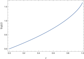
Figure 13: The dilogarithm function $\text{Li}_{2}(z)$

As we mentioned above, $J_{\phi}^{B}(M_{\phi},\mathbf{0})=0$. Therefore, we finally have

$$J_{\phi}(M_{\phi},\mathbf{0})=3J_{\phi}^{A}(M_{\phi},\mathbf{0})=\frac{3T^{2}}{\mathrm{i}\,32\pi^{3}}\,\text{Li}_{2}(\mathrm{e}^{-M_{\phi}/T})\,.$$ (B118)

Substituting the above into Eq. (B89) and using Eq. (B87), one obtains

$${\rm Im}\widetilde{\Pi}^{\rm R}_{\phi}(M_{\phi},\mathbf{0})={\rm Im}\widetilde{\pi}(M_{\phi})=-\frac{\lambda_{\phi}^{2}\,T^{2}}{128\pi^{3}}\,\text{Li}_{2}(\mathrm{e}^{-M_{\phi}/T})\,.$$ (B119)

Substituting the above into the definition of $\gamma$, one obtains Eq. (23). Eq. (B119) is the result obtained in Refs. [65, 66, 67]. For other related discussions, see, e.g., Refs. [68, 96].

B.2.2 Computation of $J_{\chi}$

Now we consider $J_{\chi}(p)$ which can be written as

$$J_{\chi}(p)= -\mathrm{i}\int\frac{\mathrm{d}^{4}k_{1}}{(2\pi)^{4}}\int\frac{\mathrm{d}^{4}k_{2}}{(2\pi)^{4}}\int\frac{\mathrm{d}^{4}k_{3}}{(2\pi)^{4}}(2\pi)^{4}\delta^{(4)}(p-k_{1}-k_{2}-k_{3})\rho_{\phi,\mathbf{k}_{1}}(k_{1,0})\rho_{\chi,\mathbf{k}_{2}}(k_{2,0})\rho_{\chi,\mathbf{k}_{3}}(k_{3,0})$$

$$\times\left\{\left[1+f_{\rm B}(k_{1,0})\right]\left[f_{\rm B}(k_{2,0})+1\right]\left[f_{\rm B}(k_{3,0})+1\right]-f_{\rm B}(k_{1,0})f_{\rm B}(k_{2,0})f_{\rm B}(k_{3,0})\right\}\,.$$ (B120)

Similar to what we have done earlier, performing the integrals over $k_{i,0}$ and relabeling the integration variables lead to

$$J_{\chi}(p)= -\mathrm{i}\int\frac{\mathrm{d}^{3}\mathbf{k}_{1}}{(2\pi)^{3}}\int\frac{\mathrm{d}^{3}\mathbf{k}_{2}}{(2\pi)^{3}}\int\frac{\mathrm{d}^{3}\mathbf{k}_{3}}{(2\pi)^{3}}(2\pi)^{4}\delta^{(3)}(\mathbf{p}-\mathbf{k}_{1}-\mathbf{k}_{2}-\mathbf{k}_{3})\frac{\mathcal{F}_{2}(p_{0},\omega_{\phi,\mathbf{k}_{1}},\omega_{\chi,\mathbf{k}_{2}},\omega_{\chi,\mathbf{k}_{3}})}{8\,\omega_{\mathbf{k}_{1}}\omega_{\mathbf{k}_{2}}\omega_{\mathbf{k}_{3}}}\,,$$ (B121)

where

$$\mathcal{F}_{2}(p_{0},\omega_{\phi,\mathbf{k}_{1}},\omega_{\chi,\mathbf{k}_{2}},\omega_{\chi,\mathbf{k}_{3}})=\Bigg{\{}\Big{[}\delta(p_{0}-\omega_{\phi,\mathbf{k}_{1}}-\omega_{\chi,\mathbf{k}_{2}}-\omega_{\chi,\mathbf{k}_{3}})-\delta(p_{0}+\omega_{\phi,\mathbf{k}_{1}}+\omega_{\chi,\mathbf{k}_{2}}+\omega_{\chi,\mathbf{k}_{3}})\Big{]}$$

$$\quad\times\bigg{(}\left[1+f_{\rm B}(\omega_{\phi,\mathbf{k}_{1}})\right]\left[f_{\rm B}(\omega_{\chi,\mathbf{k}_{2}})+1\right]\left[f_{\rm B}(\omega_{\chi,\mathbf{k}_{3}})+1\right]-f_{\rm B}(\omega_{\phi,\mathbf{k}_{1}})f_{\rm B}(\omega_{\chi,\mathbf{k}_{2}})f_{\rm B}(\omega_{\chi,\mathbf{k}_{3}})\bigg{)}$$

$$\quad+\Big{[}\delta(p_{0}-\omega_{\phi,\mathbf{k}_{1}}+\omega_{\chi,\mathbf{k}_{2}}+\omega_{\chi,\mathbf{k}_{3}})-\delta(p_{0}+\omega_{\phi,\mathbf{k}_{1}}-\omega_{\chi,\mathbf{k}_{2}}-\omega_{\chi,\mathbf{k}_{3}})\Big{]}$$

$$\quad\times\bigg{(}\left[1+f_{\rm B}(\omega_{\phi,\mathbf{k}_{1}})\right]f_{\rm B}(\omega_{\chi,\mathbf{k}_{2}})f_{\rm B}(\omega_{\chi,\mathbf{k}_{3}})-f_{\rm B}(\omega_{\phi,\mathbf{k}_{1}})[1+f_{\rm B}(\omega_{\chi,\mathbf{k}_{2}})][1+f_{\rm B}(\omega_{\chi,\mathbf{k}_{3}})]\bigg{)}$$

$$\quad+2\times\Big{[}\delta(p_{0}+\omega_{\phi,\mathbf{k}_{1}}-\omega_{\chi,\mathbf{k}_{2}}+\omega_{\chi,\mathbf{k}_{3}})-\delta(p_{0}-\omega_{\phi,\mathbf{k}_{1}}+\omega_{\chi,\mathbf{k}_{2}}-\omega_{\chi,\mathbf{k}_{3}})\Big{]}$$

$$\quad\times\bigg{(}\left[1+f_{\rm B}(\omega_{\chi,\mathbf{k}_{2}})\right]f_{\rm B}(\omega_{\phi,\mathbf{k}_{1}})f_{\rm B}(\omega_{\chi,\mathbf{k}_{3}})-f_{\rm B}(\omega_{\chi,\mathbf{k}_{2}})[1+f_{\rm B}(\omega_{\phi,\mathbf{k}_{1}})][1+f_{\rm B}(\omega_{\chi,\mathbf{k}_{3}})]\bigg{)}\Bigg{\}}\,.$$ (B122)

One can similarly interpret every $\delta$-function in terms of particle production processes.

The calculation of $J_{\chi}(p)$ is much more involved. We will restrict ourselves to $p=(M_{\phi},\mathbf{0})$ from the beginning. For $p_{0}=M_{\phi}>0$, the second $\delta$-function in Eq. (B.2.2) cannot be fulfilled. Further, since $\omega_{\phi,\mathbf{k}_{1}}\geq M_{\phi}$, the first $\delta$-function cannot be fulfilled either. Using Eq. (B95) and after some simple algebra, one can show that the third and fifth $\delta$-functions cannot be fulfilled. Therefore, the only processes that can be on-shell are

$$\varphi\phi_{1}\leftrightarrow\chi_{2}\chi_{3}\;\;\text{and}\;\;\varphi\chi_{2}\leftrightarrow\phi_{1}\chi_{3}\,,$$ (B123)

corresponding to the fourth and sixth $\delta$-functions.

Using $1+f_{\rm B}(\omega_{\mathbf{k}})=\exp(\beta\omega_{\mathbf{k}})f_{\rm B}(\omega_{\mathbf{k}})$, one can write $J_{\chi}(M_{\phi},\mathbf{0})$ as

$$J_{\chi}(M_{\phi},\mathbf{0})=J^{A}_{\chi}(M_{\phi},\mathbf{0})+2J^{B}_{\chi}(M_{\phi},\mathbf{0})\,,$$ (B124)

where

$$J^{A}_{\chi}(M_{\phi},\mathbf{0})= -\mathrm{i}\left(\mathrm{e}^{\beta p_{0}}-1\right)\int\frac{\mathrm{d}^{3}\mathbf{k}_{1}}{(2\pi)^{3}}\int\frac{\mathrm{d}^{3}\mathbf{k}_{2}}{(2\pi)^{3}}\int\frac{\mathrm{d}^{3}\mathbf{k}_{3}}{(2\pi)^{3}}\frac{(2\pi)^{4}\delta^{(3)}(\mathbf{k}_{1}+\mathbf{k}_{2}+\mathbf{k}_{3})}{8\,\omega_{\phi,\mathbf{k}_{1}}\omega_{\chi,\mathbf{k}_{2}}\omega_{\chi,\mathbf{k}_{3}}}$$

$$\times\delta(M_{\phi}+\omega_{\phi,\mathbf{k}_{1}}-\omega_{\chi,\mathbf{k}_{2}}-\omega_{\chi,\mathbf{k}_{3}})\times\left[1+f_{\rm B}(\omega_{\phi,\mathbf{k}_{1}})\right]f_{\rm B}(\omega_{\chi,\mathbf{k}_{2}})f_{\rm B}(\omega_{\chi,\mathbf{k}_{3}})\,,$$ (B125)

and

$$J^{B}_{\chi}(M_{\phi},\mathbf{0})= -\mathrm{i}\left(\mathrm{e}^{\beta p_{0}}-1\right)\int\frac{\mathrm{d}^{3}\mathbf{k}_{1}}{(2\pi)^{3}}\int\frac{\mathrm{d}^{3}\mathbf{k}_{2}}{(2\pi)^{3}}\int\frac{\mathrm{d}^{3}\mathbf{k}_{3}}{(2\pi)^{3}}\frac{(2\pi)^{4}\delta^{(3)}(\mathbf{k}_{1}+\mathbf{k}_{2}+\mathbf{k}_{3})}{8\,\omega_{\phi,\mathbf{k}_{1}}\omega_{\chi,\mathbf{k}_{2}}\omega_{\chi,\mathbf{k}_{3}}}$$

$$\times\delta(M_{\phi}+\omega_{\chi,\mathbf{k}_{2}}-\omega_{\phi,\mathbf{k}_{1}}-\omega_{\chi,\mathbf{k}_{3}})\times\left[1+f_{\rm B}(\omega_{\chi,\mathbf{k}_{2}})\right]f_{\rm B}(\omega_{\phi,\mathbf{k}_{1}})f_{\rm B}(\omega_{\chi,\mathbf{k}_{3}})\,.$$ (B126)

In the following, we calculate $J^{A}_{\chi}(M_{\phi},\mathbf{0})$ and $J^{B}_{\chi}(M_{\phi},\mathbf{0})$, separately.

$J^{A}_{\chi}(M_{\phi},\mathbf{0})$

Performing the integrals over $\mathbf{k}_{3}$ in Eq. (B.2.2), we obtain

$$J^{A}_{\chi}(M_{\phi},\mathbf{0})= -2\pi\mathrm{i}\left(\mathrm{e}^{\beta M_{\phi}}-1\right)\int\frac{\mathrm{d}^{3}\mathbf{k}_{1}}{(2\pi)^{3}}\int\frac{\mathrm{d}^{3}\mathbf{k}_{2}}{(2\pi)^{3}}\frac{\delta(M_{\phi}+\omega_{\phi,\mathbf{k}_{1}}-\omega_{\chi,\mathbf{k}_{2}}-\omega_{\chi,\mathbf{k}_{1}+\mathbf{k}_{2}})}{8\,\omega_{\phi,\mathbf{k}_{1}}\omega_{\chi,\mathbf{k}_{2}}\omega_{\chi,\mathbf{k}_{1}+\mathbf{k}_{2}}}$$ (B127)

$$\times\left[1+f_{\rm B}(\omega_{\phi,\mathbf{k}_{1}})\right]f_{\rm B}(\omega_{\chi,\mathbf{k}_{2}})f_{\rm B}(\omega_{\chi,\mathbf{k}_{1}+\mathbf{k}_{2}})\,.$$

To perform the $\mathbf{k}_{2}$ integration, we use spherical coordinates with $\mathbf{k}_{1}$ being the polar axis ($\theta=0$). Then,

$$J^{A}_{\chi}(M_{\phi},\mathbf{0})= -2\pi\mathrm{i}\left(\mathrm{e}^{\beta M_{\phi}}-1\right)\int\frac{\mathrm{d}^{3}\mathbf{k}_{1}}{(2\pi)^{3}}\int_{0}^{\infty}\frac{\mathrm{d}|\mathbf{k}_{2}|\,|\mathbf{k}_{2}|^{2}}{(2\pi)^{2}}\int^{1}_{-1}\mathrm{d}\cos\theta$$ (B128)

$$\times\frac{\delta(M_{\phi}+\omega_{\phi,\mathbf{k}_{1}}-\omega_{\chi,\mathbf{k}_{2}}-\omega_{\chi,\mathbf{k}_{1}+\mathbf{k}_{2}})}{8\,\omega_{\phi,\mathbf{k}_{1}}\omega_{\chi,\mathbf{k}_{2}}\omega_{\chi,\mathbf{k}_{1}+\mathbf{k}_{2}}}\left[1+f_{\rm B}(\omega_{\phi,\mathbf{k}_{1}})\right]f_{\rm B}(\omega_{\chi,\mathbf{k}_{2}})f_{\rm B}(\omega_{\chi,\mathbf{k}_{1}+\mathbf{k}_{2}})\,.$$

Since $-1\leq\cos\theta\leq 1$, the $\delta$-function requires that

$$\sqrt{M^{2}_{\chi}+\left(|\mathbf{k}_{1}|-|\mathbf{k}_{2}|\right)^{2}}\leq M_{\phi}+\omega_{\phi,\mathbf{k}_{1}}-\omega_{\chi,\mathbf{k}_{2}}\leq\sqrt{M^{2}_{\chi}+\left(|\mathbf{k}_{1}|+|\mathbf{k}_{2}|\right)^{2}}\,,$$ (B129)

which can be reduced to

$$\omega_{\chi,\mathbf{k}_{2}}\leq M_{\phi}+\omega_{\phi,\mathbf{k}_{1}}\,,$$ (B130a)

$$\Big{|}(M_{\phi}+\omega_{\phi,\mathbf{k}_{1}}-\omega_{\chi,\mathbf{k}_{2}})^{2}-(\omega_{\phi,\mathbf{k}_{1}}^{2}+\omega_{\chi,\mathbf{k}_{2}}^{2}-M_{\phi}^{2})\Big{|}\leq 2|\mathbf{k}_{1}||\mathbf{k}_{2}|\,.$$ (B130b)

Taking the square of Eq. (B130b) gives

$$\Sigma_{1}\omega_{\chi,\mathbf{k}_{2}}^{2}+\Sigma_{2}\omega_{\chi,\mathbf{k}_{2}}+\Sigma_{3}\leq 0\,,$$ (B131)

where

$$\Sigma_{1} =8M_{\phi}\left(M_{\phi}+\omega_{\phi,\mathbf{k}_{1}}\right)\,,$$ (B132)

$$\Sigma_{2} =-8M_{\phi}\left(M_{\phi}+\omega_{\phi,\mathbf{k}_{1}}\right)^{2}\,,$$ (B133)

$$\Sigma_{3} =4\left(M_{\phi}+\omega_{\phi,\mathbf{k}_{1}}\right)\left(M^{3}_{\phi}-M_{\phi}M^{2}_{\chi}+M_{\phi}^{2}\omega_{\phi,\mathbf{k}_{1}}+M_{\chi}^{2}\omega_{\phi,\mathbf{k}_{1}}\right)\,.$$ (B134)

Since $\Sigma_{1}>0$, the condition (B131) is equivalent to

$$-2M_{\chi}^{2}+M_{\phi}^{2}+M_{\phi}\omega_{\phi,\mathbf{k}_{1}}>0\,,$$ (B135a)

$$\Omega^{-}_{2}\leq\omega_{\chi,\mathbf{k}_{2}}\leq\Omega^{+}_{2}\,,$$ (B135b)

where

$$\Omega^{\pm}_{2}=\frac{M_{\phi}(M_{\phi}+\omega_{\phi,\mathbf{k}_{1}})\pm\sqrt{M_{\phi}(\omega_{\phi,\mathbf{k}_{1}}-M_{\phi})(-2M_{\chi}^{2}+M_{\phi}^{2}+M_{\phi}\omega_{\phi,\mathbf{k}_{1}})}}{2M_{\phi}}\,.$$ (B136)

To have $\Omega^{+}_{2}>M_{\chi}$, we require

$$M_{\phi}(M_{\phi}+\omega_{\phi,\mathbf{k}_{1}}-2M_{\chi})+\sqrt{M_{\phi}(\omega_{\phi,\mathbf{k}_{1}}-M_{\phi})(-2M_{\chi}^{2}+M_{\phi}^{2}+M_{\phi}\omega_{\phi,\mathbf{k}_{1}})}>0\,.$$ (B137)

If

$$\omega_{\phi,\mathbf{k}_{1}}>2M_{\chi}-M_{\phi}\,,$$ (B138)

The condition (B137) is satisfied automatically. If $\omega_{\phi,\mathbf{k}_{1}}<2M_{\chi}-M_{\phi}$, then the condition (B137) requires

$$M_{\phi}(\omega_{\phi,\mathbf{k}_{1}}-M_{\phi})(-2M_{\chi}^{2}+M_{\phi}^{2}+M_{\phi}\omega_{\phi,\mathbf{k}_{1}})>\left[M_{\phi}(M_{\phi}+\omega_{\phi,\mathbf{k}_{1}}-2M_{\chi})\right]^{2}\,.$$ (B139)

The above condition can be simplified to $(M_{\chi}-M_{\phi})^{2}M_{\phi}(M_{\phi}+\omega_{\phi,\mathbf{k}_{1}})<0$ which cannot be fulfilled. Therefore, we have the requirement (B138) to ensure $\Omega_{2}^{+}>M_{h}$. It also can be shown that

$$\Omega^{+}_{2}<M_{\phi}+\omega_{\phi,\mathbf{k}_{1}}-M_{\chi}\,,$$ (B140)

such that the condition (B130a) is automatically satisfied when Eq. (B135b) is fulfilled. On the other hand, one can show that

$$\Omega^{-}_{2}=\frac{M_{\phi}+\omega_{\phi,\mathbf{k}_{1}}}{2}-\frac{1}{2}\sqrt{\left(\omega_{\phi,\mathbf{k}_{1}}-\frac{M_{\chi}^{2}}{M_{\phi}}\right)^{2}-\left(\frac{M^{2}_{\chi}}{M_{\phi}}-M_{\phi}\right)^{2}}\geq\frac{1}{2}\left(M_{\phi}+\frac{M^{2}_{\chi}}{M_{\phi}}\right)\geq M_{\chi}\,.$$ (B141)

In conclusion, the integral over $\cos\theta$ in Eq. (B128) gives the following constraint

$$\omega_{\phi,\mathbf{k}_{1}}\geq\Omega^{-}_{1}\,,$$ (B142a)

$$\Omega^{-}_{2}\leq\omega_{\chi,\mathbf{k}_{2}}\leq\Omega^{+}_{2}\,,$$ (B142b)

where

$$\Omega^{-}_{1}=\max[M_{\phi},(2M_{\chi}^{2}-M_{\phi}^{2})/M_{\phi},2M_{\chi}-M_{\phi}]=\max[M_{\phi},(2M_{\chi}^{2}-M_{\phi}^{2})/M_{\phi}]\,.$$ (B143)

Similarly, introducing spherical coordinates for $\mathbf{k}_{1}$ and doing the integral over the angular coordinates gives

$$J^{A}_{\chi}(M_{\phi},\mathbf{0})= \frac{\left(\mathrm{e}^{\beta M_{\phi}}-1\right)}{\mathrm{i}\,32\pi^{3}}\int^{\infty}_{\Omega^{-}_{1}}\mathrm{d}\omega_{\phi,\mathbf{k}_{1}}\int_{\Omega^{-}_{2}}^{{\Omega^{+}_{2}}}\mathrm{d}\omega_{\chi,\mathbf{k}_{2}}\left[1+f_{\rm B}(\omega_{\phi,\mathbf{k}_{1}})\right]f_{\rm B}(\omega_{\chi,\mathbf{k}_{2}})f_{\rm B}(M_{\phi}+\omega_{\phi,\mathbf{k}_{1}}-\omega_{\chi,\mathbf{k}_{2}})\,.$$ (B144)

Doing the integral over $\omega_{\mathbf{k}_{2}}$, we obtain

$$J^{A}_{\chi}(M_{\phi},\mathbf{0})= \frac{\mathrm{e}^{\beta M_{\phi}}-1}{\mathrm{i}\,32\pi^{3}\beta}\int^{\infty}_{\Omega^{-}_{1}}\mathrm{d}\omega_{\phi,\mathbf{k}_{1}}[1+f_{\rm B}(\omega_{\phi,\mathbf{k}_{1}})]f_{\rm B}(M_{\phi}+\omega_{\phi,\mathbf{k}_{1}})$$

$$\qquad\qquad\qquad\times\ln\left[\frac{\left(\mathrm{e}^{\beta\Omega^{+}_{2}}-1\right)\left(\mathrm{e}^{\beta(M_{\phi}+\omega_{\phi,\mathbf{k}_{1}})}-\mathrm{e}^{\beta\Omega_{2}^{-}}\right)}{\left(\mathrm{e}^{\beta(M_{\phi}+\omega_{\phi,\mathbf{k}_{1}})}-\mathrm{e}^{\beta\Omega_{2}^{+}}\right)\left(\mathrm{e}^{\beta\Omega^{-}_{2}}-1\right)}\right]\,.$$ (B145)

For $M_{\phi}=M_{\chi}$, we have $J^{A}_{\chi}(M_{\phi},\mathbf{0})=J^{A}_{\phi}(M_{\phi},\mathbf{0})$. For general $M_{\chi}$, there is no a closed form of $J^{A}_{\chi}(M_{\phi},\mathbf{0})$. Numerical results of $J^{A}_{\chi}(M_{\phi},\mathbf{0})$ for different values of $M_{\chi}/M_{\phi}$ are shown in Fig. 14.

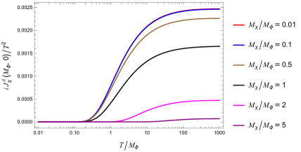
Figure 14: Numerical results for $J^{A}_{\chi}(M_{\phi},\mathbf{0})$. Note that the red and blue curves are overlapped, indicating that for $M_{\chi}\;\raisebox{-2.70003pt}{$\stackrel{{\scriptstyle\displaystyle<}}{{\sim}}$}\;0.1M_{\phi}$ the integral depends very weekly on $M_{\chi}/M_{\phi}$.

In order to have an analytic expression for $J_{\chi}^{A}(M_{\phi},\mathbf{0})$, we do the fitting using the known function $J^{A}_{\phi}(M_{\phi},\mathbf{0})$,

$$J_{\chi}^{A}(M_{\phi},\mathbf{0})\sim J_{\chi,\rm fit}^{A}(M_{\phi},\mathbf{0})\equiv 1.49\times\frac{6}{\pi^{2}}\times{\rm Li}_{2}\left(\frac{4}{(M_{\chi}/M_{\phi})^{3}+4}\right)J_{\phi}^{A}\left(\frac{M_{\chi}+2M_{\phi}}{3},\mathbf{0}\right)\,.$$ (B146)

The comparison between this fit function and the exact numerical results is shown in Fig. 15.

Figure 15: Comparison between the fit function $J_{\chi,\rm fit}^{A}(M_{\phi},\mathbf{0})$ (dashed lines) and exact numerical results of $J_{\chi}^{A}(M_{\phi},\mathbf{0})$ (solid lines).

$J^{B}_{\chi}(M_{\phi},\mathbf{0})$

Performing the integrals over $\mathbf{k}_{3}$ in Eq. (B.2.2), we obtain

$$J^{B}_{\chi}(M_{\phi},\mathbf{0})= -2\pi\mathrm{i}\left(\mathrm{e}^{\beta M_{\phi}}-1\right)\int\frac{\mathrm{d}^{3}\mathbf{k}_{2}}{(2\pi)^{3}}\int\frac{\mathrm{d}^{3}\mathbf{k}_{1}}{(2\pi)^{3}}\frac{\delta(M_{\phi}+\omega_{\chi,\mathbf{k}_{2}}-\omega_{\phi,\mathbf{k}_{1}}-\omega_{\chi,\mathbf{k}_{1}+\mathbf{k}_{2}})}{8\,\omega_{\phi,\mathbf{k}_{1}}\omega_{\chi,\mathbf{k}_{2}}\omega_{\chi,\mathbf{k}_{1}+\mathbf{k}_{2}}}$$ (B147)

$$\times\left[1+f_{\rm B}(\omega_{\chi,\mathbf{k}_{2}})\right]f_{\rm B}(\omega_{\phi,\mathbf{k}_{1}})f_{\rm B}(\omega_{\chi,\mathbf{k}_{1}+\mathbf{k}_{2}})\,.$$

Different from the earlier calculations, we now perform the integral over $\mathbf{k}_{1}$ first. To do that, we introduce spherical coordinates for $\mathbf{k}_{1}$ with $\mathbf{k}_{2}$ being the polar axis ($\theta=0$). Then,

$$J^{B}_{\chi}(M_{\phi},\mathbf{0})= -2\pi\mathrm{i}\left(\mathrm{e}^{\beta M_{\phi}}-1\right)\int\frac{\mathrm{d}^{3}\mathbf{k}_{2}}{(2\pi)^{3}}\int_{0}^{\infty}\frac{\mathrm{d}|\mathbf{k}_{1}|\,|\mathbf{k}_{1}|^{2}}{(2\pi)^{2}}\int^{1}_{-1}\mathrm{d}\cos\theta$$

$$\times\frac{\delta(M_{\phi}+\omega_{\chi,\mathbf{k}_{2}}-\omega_{\phi,\mathbf{k}_{1}}-\omega_{\chi,\mathbf{k}_{1}+\mathbf{k}_{2}})}{8\,\omega_{\phi,\mathbf{k}_{1}}\omega_{\chi,\mathbf{k}_{2}}\omega_{\chi,\mathbf{k}_{1}+\mathbf{k}_{2}}}\left[1+f_{\rm B}(\omega_{\chi,\mathbf{k}_{2}})\right]f_{\rm B}(\omega_{\phi,\mathbf{k}_{1}})f_{\rm B}(\omega_{\chi,\mathbf{k}_{1}+\mathbf{k}_{2}})\,.$$ (B148)

The $\delta$-function is satisfied when

$$M_{\phi}+\omega_{\chi,\mathbf{k}_{2}}-\omega_{\phi,\mathbf{k}_{1}}-\sqrt{M^{2}_{\chi}+|\mathbf{k}_{1}|^{2}+|\mathbf{k}_{2}|^{2}+2|\mathbf{k}_{1}||\mathbf{k}_{2}|\cos\theta}=0\,.$$ (B149)

Since $-1\leq\cos\theta\leq 1$, Eq. (B149) requires that

$$\sqrt{M^{2}_{\chi}+\left(|\mathbf{k}_{1}|-|\mathbf{k}_{2}|\right)^{2}}\leq M_{\phi}+\omega_{\chi,\mathbf{k}_{2}}-\omega_{\phi,\mathbf{k}_{1}}\leq\sqrt{M^{2}_{\chi}+\left(|\mathbf{k}_{1}|+|\mathbf{k}_{2}|\right)^{2}}\,,$$ (B150)

which can be reduced to

$$\omega_{\phi,\mathbf{k}_{1}}\leq M_{\phi}+\omega_{\chi,\mathbf{k}_{2}}\,,$$ (B151a)

$$\Big{|}(M_{\phi}+\omega_{\chi,\mathbf{k}_{2}}-\omega_{\phi,\mathbf{k}_{1}})^{2}-(\omega_{\phi,\mathbf{k}_{1}}^{2}+\omega_{\chi,\mathbf{k}_{2}}^{2}-M_{\phi}^{2})\Big{|}\leq 2|\mathbf{k}_{1}||\mathbf{k}_{2}|\,.$$ (B151b)

Taking the square of Eq. (B151b) gives

$$\Sigma_{1}\omega_{\phi,\mathbf{k}_{1}}^{2}+\Sigma_{2}\omega_{\phi,\mathbf{k}_{1}}+\Sigma_{3}\leq 0\,,$$ (B152)

where

$$\Sigma_{1} =4\left(M_{\phi}^{2}+M_{\chi}^{2}+2M_{\phi}\omega_{\chi,\mathbf{k}_{2}}\right)\,,$$ (B153)

$$\Sigma_{2} =-8M_{\phi}\left(M_{\phi}+\omega_{\chi,\mathbf{k}_{2}}\right)^{2}\,,$$ (B154)

$$\Sigma_{3} =4M_{\phi}^{2}\left(M^{2}_{\phi}-M_{\chi}^{2}+2M_{\phi}\omega_{\chi,\mathbf{k}_{2}}+2\omega^{2}_{\chi,\mathbf{k}_{2}}\right)\,.$$ (B155)

Since $\Sigma_{1}>0$, condition Eq. (B152) gives

$$\Omega^{-}_{1}\leq\omega_{\phi,\mathbf{k}_{1}}\leq\Omega^{+}_{1}\,,$$ (B156)

where

$$\Omega^{-}_{1} =M_{\phi}\,,$$ (B157)

$$\Omega^{+}_{1} =\frac{M_{\phi}(M_{\phi}^{2}-M_{\chi}^{2}+2M_{\phi}\omega_{\chi,\mathbf{k}_{2}}+2\omega_{\chi,\mathbf{k}_{2}}^{2})}{M_{\phi}^{2}+M_{\chi}^{2}+2M_{\phi}\omega_{\chi,\mathbf{k}_{2}}}\,.$$ (B158)

It can be shown that

$$\Omega^{+}_{1}\leq M_{\phi}+\omega_{\chi,\mathbf{k}_{2}}-M_{\chi}\,,$$ (B159)

so that Eq. (B151a) is automatically satisfied when $\omega_{\phi,\mathbf{k}_{1}}\leq\Omega_{1}^{+}$.

In conclusion, the integral over $\cos\theta$ in Eq. (B.2) gives the following constraint

$$\omega_{\chi,\mathbf{k}_{2}}\geq M_{\chi}\,,\qquad\Omega^{-}_{1}\leq\omega_{\phi,\mathbf{k}_{1}}\leq\Omega^{+}_{1}\,.$$ (B160)

Then, we have

$$J^{B}_{\chi}(M_{\phi},\mathbf{0})= \frac{\left(\mathrm{e}^{\beta M_{\phi}}-1\right)}{\mathrm{i}\,32\pi^{3}}\int^{\infty}_{M_{\chi}}\mathrm{d}\omega_{\chi,\mathbf{k}_{2}}\int_{\Omega^{-}_{1}}^{{\Omega^{+}_{1}}}\mathrm{d}\omega_{\phi,\mathbf{k}_{1}}\left[1+f_{\rm B}(\omega_{\chi,\mathbf{k}_{2}})\right]f_{\rm B}(\omega_{\phi,\mathbf{k}_{1}})f_{\rm B}(M_{\phi}+\omega_{\chi,\mathbf{k}_{2}}-\omega_{\phi,\mathbf{k}_{1}})\,.$$ (B161)

Doing the integral over $\omega_{\phi,\mathbf{k}_{1}}$, one arrives at

$$J^{B}_{\chi}(M_{\phi},\mathbf{0})= \frac{\mathrm{e}^{\beta M_{\phi}}-1}{\mathrm{i}\,32\pi^{3}\beta}\int^{\infty}_{M_{\chi}}\mathrm{d}\omega_{\chi,\mathbf{k}_{2}}[1+f_{\rm B}(\omega_{\chi,\mathbf{k}_{2}})]f_{\rm B}(M_{\phi}+\omega_{\chi,\mathbf{k}_{2}})$$

$$\qquad\times\ln\left[\frac{\left(\mathrm{e}^{\beta\Omega^{+}_{1}}-1\right)\left(\mathrm{e}^{\beta(M_{\phi}+\omega_{\chi,\mathbf{k}_{2}})}-\mathrm{e}^{\beta\Omega_{1}^{-}}\right)}{\left(\mathrm{e}^{\beta(M_{\phi}+\omega_{\chi,\mathbf{k}_{2}})}-\mathrm{e}^{\beta\Omega_{1}^{+}}\right)\left(\mathrm{e}^{\beta\Omega^{-}_{1}}-1\right)}\right]\,.$$ (B162)

For $M_{\phi}=M_{\chi}$, we have $J^{B}_{\chi}(M_{\phi},\mathbf{0})=J^{A}_{\phi}(M_{\phi},\mathbf{0})$. For general $M_{\chi}$, the expressions for $\Omega^{\pm}_{1}$ are too complicated to evaluate a closed form of $J^{B}_{\chi}(M_{\phi},\mathbf{0})$. Numerical results of $J^{B}_{\chi}(M_{\phi},\mathbf{0})$ for different values of $M_{\chi}/M_{\phi}$ are shown in Fig. 16.

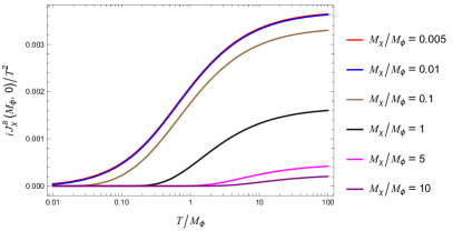
Figure 16: Numerical results of $J^{B}_{\chi}(M_{\phi},\mathbf{0})$. Note that the red and blue curves are almost overlapped, indicating that for $M_{\chi}\;\raisebox{-2.70003pt}{$\stackrel{{\scriptstyle\displaystyle<}}{{\sim}}$}\;0.01M_{\phi}$ the integral depends very weekly on $M_{\chi}/M_{\phi}$.

We use the following function to approximate $J_{h}^{B}(M_{\phi},\mathbf{0})$,

$$J_{\chi}^{B}(M_{\phi},\mathbf{0})\sim J_{\chi,\rm fit}^{B}(M_{\phi},\mathbf{0})\equiv 2.28\times\frac{6}{\pi^{2}}\times{\rm Li}_{2}\left(\frac{1.6}{(M_{\chi}/M_{\phi})+1.6}\right)J^{A}_{\phi}\left(\frac{2M_{\chi}+M_{\phi}}{3},\mathbf{0}\right)\,.$$ (B163)

The comparison between this fit function and the exact numerical results is shown in Fig. 17.

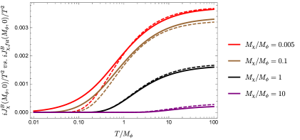
Figure 17: Comparison between the fit function $J_{\chi,\rm fit}^{B}(M_{\phi},\mathbf{0})$ (dashed lines) and exact numerical results of $J_{\chi}^{B}(M_{\phi},\mathbf{0})$ (solid lines).

Appendix C Solving the condensate equation of motion with a time-dependent mass term

The condensate EoM (7) has been solved in Refs. [36, 44] for constant $M_{\phi}$ using the multi-scale analysis [34, 35]. In this section, we solve it when $M_{\phi}$ is time-dependent but adiabatic, $\dot{M}_{\phi}/M_{\phi}^{2}\ll 1$.

As a standard procedure for perturbation theory, one puts a bookkeeping parameter $\varepsilon$ in front of all perturbatively small terms in the EoM. When doing the perturbative expansion, the higher power of $\varepsilon$ a quantity is associated with, the smaller the quantity is. Therefore, we have

$$\ddot{\varphi}(t)+M_{\phi}^{2}\varphi(t)+3\varepsilon H\dot{\varphi}(t)+\varepsilon\frac{\lambda_{\phi}\varphi^{3}(t)}{6}+\varepsilon\int_{t_{i}}^{t}\mathrm{d}t^{\prime}\,\pi_{\rm R}(t-t^{\prime})\varphi(t^{\prime})+\varepsilon\frac{\varphi(t)}{6}\int_{t_{i}}^{t}\mathrm{d}t^{\prime}\,v_{\rm R}(t-t^{\prime})\varphi^{2}(t^{\prime})=0\,.$$ (C164)

There is a hierarchy in the time scales in the evolution of the condensate. The shorter time scale corresponds to the oscillation frequency, and the longer time scale corresponds to the damping rate. One can understand this by imaging a form of the condensate evolution $\varphi(t)=A(t)B(t)$ where $B(t)$ is an oscillating function and $A(t)$ is the envelope function. One can expect that

$$M_{\phi}\sim\frac{1}{B(t)}\frac{\mathrm{d}B(t)}{\mathrm{d}t}\gg\frac{1}{A(t)}\frac{\mathrm{d}A(t)}{\mathrm{d}t}\sim\varepsilon M_{\phi}\,.$$ (C165)

Therefore, when taking time derivatives of $\varphi$, one can obtain quantities at different orders in $\varepsilon$. In order to trace these quantities, we thus formally introduce two different time variables. In the above example, one can write it as $\varphi(t,\tau)=A(\tau)B(t)$ with $\tau=\varepsilon t$. Then we have

$$\frac{\mathrm{d}\varphi}{\mathrm{d}t}=\frac{\mathrm{d}\tau}{\mathrm{d}t}\frac{\partial\varphi(t,\tau)}{\partial\tau}+\frac{\partial\varphi(t,\tau)}{\partial t}=\varepsilon\frac{\mathrm{d}A(\tau)}{\mathrm{d}\tau}B(t)+A(\tau)\frac{\mathrm{d}B(t)}{\mathrm{d}t}\,.$$ (C166)

This way, the smaller term is now associated with a factor $\varepsilon$. These two-time variables are used when solving the above equation for constant $M_{\phi}$.

Here we consider a slowly evolving $M_{\phi}(\tau)$ where $\tau$ is still the slow time variable. It turns out that in this case the fast time variable now is [35]

$$\eta=f(t)=\int^{t}\mathrm{d}t^{\prime}M_{\phi}(\varepsilon t^{\prime})\,.$$ (C167)

We shall see shortly the advantage of introducing the $\eta$ time variable. We will also assume $H=H(\tau)$.

Now let $\varphi$ take the following form

$$\varphi(t)=\varphi(t,\tau;\varepsilon)=\varphi_{0}(t,\tau)+\varepsilon\varphi_{1}(t,\tau)+\varepsilon^{2}\varphi_{2}(t,\tau)+...\,,$$ (C168)

where

$$\varphi_{n}(t,\tau)=\frac{1}{n!}\frac{\partial^{n}\varphi(t,\tau;\varepsilon)}{\partial\varepsilon^{n}}\bigg{|}_{\varepsilon=0}$$ (C169)

are the coefficients. Below, we will still use the time variable $t$ inside the integrals which then should be understood as $t=f^{-1}(\eta)$. Now one can directly expand the first four terms of Eq. (C164) in powers of $\varepsilon$. To expand the non-local terms of Eq. (C164) in powers of $\varepsilon$, we need some simplification. Assuming that the solution for the condensate $\varphi$ varies only slightly during the window provided by the kernel of the non-local terms, we can Taylor-expand $\varphi(t^{\prime},\tau^{\prime};\varepsilon)$ at $\tau$ as

$$\varphi(t^{\prime},\tau^{\prime};\varepsilon)=\varphi(t^{\prime},\tau;\varepsilon)+\varepsilon(t^{\prime}-t)\frac{\partial\varphi(t^{\prime},\tau;\varepsilon)}{\partial\tau}+\frac{\varepsilon^{2}}{2}(t^{\prime}-t)^{2}\frac{\partial^{2}\varphi(t^{\prime},\tau;\varepsilon)}{\partial\tau^{2}}+...\,.$$ (C170)

Then, up to the second order in $\varepsilon$, the non-local terms could be written as

$$\varepsilon\int_{t_{i}}^{t} \mathrm{d}t^{\prime}\,\pi_{\rm R}(t-t^{\prime})\varphi(t^{\prime},\tau^{\prime};\varepsilon)$$

$$=\varepsilon\int_{t_{i}}^{t}\mathrm{d}t^{\prime}\,\pi_{\rm R}(t-t^{\prime})\varphi(t^{\prime},\tau;\varepsilon)-\varepsilon^{2}\int_{t_{i}}^{t}\mathrm{d}t^{\prime}\,(t-t^{\prime})\pi_{\rm R}(t-t^{\prime})\frac{\partial\varphi(t^{\prime},\tau;\varepsilon)}{\partial\tau}+\mathcal{O}(\varepsilon^{3})\,,$$ (C171)

and

$$\varepsilon\frac{\varphi(\eta,\tau;\varepsilon)}{6}\int_{t_{i}}^{t}\mathrm{d}t^{\prime}\,v_{\rm R}(t-t^{\prime})\varphi^{2}(t^{\prime},\tau^{\prime};\varepsilon)=\varepsilon\frac{\varphi(\eta,\tau;\varepsilon)}{6}\int_{t_{i}}^{t}\mathrm{d}t^{\prime}\,v_{\rm R}(t-t^{\prime})\varphi^{2}(t^{\prime},\tau;\varepsilon)$$

$$\qquad\qquad\qquad\qquad-\varepsilon^{2}\frac{\varphi(\eta,\tau;\varepsilon)}{3}\int_{t_{i}}^{t}\mathrm{d}t^{\prime}\,(t-t^{\prime})v_{\rm R}(t-t^{\prime})\varphi(t^{\prime},\tau;\varepsilon)\frac{\partial\varphi(t^{\prime},\tau;\varepsilon)}{\partial\tau}+\mathcal{O}(\varepsilon^{3})\,.$$ (C172)

Now, we are able to organize Eq. (C164) in powers of $\varepsilon$. At the leading order $\mathcal{O}(\varepsilon^{0})$, we have

$$\frac{\partial^{2}\varphi_{0}(\eta,\tau)}{\partial\eta^{2}}+\varphi_{0}(t,\tau)=0\,,$$ (C173)

which has the solution

$$\varphi_{0}(\tau,t)={\rm Re}\left[R(\tau)\mathrm{e}^{-\mathrm{i}\eta}\right]\,.$$ (C174)

Here, we see that using the time variable $\eta$, the leading-order equation takes the simple form of an equation of motion of a harmonic oscillator. $R(\tau)$ can only be determined when one looks into the equation at the order $\mathcal{O}(\varepsilon)$, which reads

$$M_{\phi}^{2}\left[\frac{\partial^{2}\varphi_{1}(\eta,\tau)}{\partial\eta^{2}}+\varphi_{1}(\eta,\tau)\right]=-2M(\tau)\frac{\partial^{2}\varphi_{0}(\eta,\tau)}{\partial\eta\partial\tau}-\frac{\mathrm{d}M_{\phi}(\tau)}{\mathrm{d}\tau}\frac{\partial\varphi_{0}(\eta,\tau)}{\partial\eta}-3H(\tau)M(\tau)\frac{\partial\varphi_{0}(\eta,\tau)}{\partial\eta}$$

$$-\frac{\lambda_{\phi}}{6}\varphi_{0}^{3}(\eta,\tau)-\int_{t_{i}}^{t}\mathrm{d}t^{\prime}\,\pi_{\rm R}(t-t^{\prime})\varphi_{0}(t^{\prime},\tau)-\frac{\varphi_{0}(\eta,\tau)}{6}\int_{t_{i}}^{t}\mathrm{d}t^{\prime}\,v_{\rm R}(t-t^{\prime})\varphi_{0}^{2}(t^{\prime},\tau)\,.$$ (C175)

The non-local terms in Eq. (C175) can be written as

$$-\int_{t_{i}}^{t}\mathrm{d}t^{\prime}\,\pi_{\rm R}(t-t^{\prime})\varphi_{0}(t^{\prime},\tau)= -\text{Re}\left[R(\tau)\mathrm{e}^{-\mathrm{i}\eta}\int_{t_{i}}^{t}\mathrm{d}t^{\prime}\,\pi_{\rm R}(t-t^{\prime})\mathrm{e}^{\mathrm{i}\int^{t}_{t^{\prime}}d\tilde{t}\,M_{\phi}(\varepsilon\tilde{t})}\right]\,,$$ (C176)

and

$$-\frac{\varphi_{0}(\eta,\tau)}{6}\int_{t_{i}}^{t}\mathrm{d}t^{\prime}\,v_{\rm R}(t-t^{\prime})\varphi_{0}^{2}(t^{\prime},\tau)=-\frac{1}{12}\text{Re}\left[\mathrm{e}^{-\mathrm{i}\eta}[R(\tau)]^{2}R^{*}(\tau)\int_{t_{i}}^{t}\mathrm{d}t^{\prime}\,v_{\rm R}(t-t^{\prime})\right]$$

$$\qquad\qquad\qquad\qquad\qquad-\frac{1}{24}\text{Re}\left[\mathrm{e}^{-\mathrm{i}\eta}[R(\tau)]^{2}R^{*}(\tau)\int_{t_{i}}^{t}\mathrm{d}t^{\prime}\,v_{\rm R}(t-t^{\prime})\mathrm{e}^{2\mathrm{i}\int^{t}_{t^{\prime}}\mathrm{d}\tilde{t}\,M_{\phi}(\varepsilon\tilde{t})}\right]$$

$$\qquad\qquad\qquad\qquad\qquad-\frac{1}{24}\text{Re}\left[\mathrm{e}^{-3\mathrm{i}\eta}[R(\tau)]^{3}\int_{t_{i}}^{t}\mathrm{d}t^{\prime}\,v_{\rm R}(t-t^{\prime})\mathrm{e}^{2\mathrm{i}\int^{t}_{t^{\prime}}\mathrm{d}\tilde{t}\,M_{\phi}(\varepsilon\tilde{t})}\right]\,.$$ (C177)

Taking into account that the kernels of the non-local terms only extend over several oscillation periods, one can make further simplifications. First, one can neglect any early-time transient effects due to initial conditions in the non-local terms by taking $t_{i}\rightarrow-\infty$. Second, the following approximation could be made (also for the corresponding term with $v_{\rm R}$)

$$\int_{t_{i}}^{t}\mathrm{d}t^{\prime}\,\pi_{\rm R}(t-t^{\prime})\mathrm{e}^{\mathrm{i}\int^{t}_{t^{\prime}}\mathrm{d}\tilde{t}\,M_{\phi}(\varepsilon\tilde{t})} \approx\int_{t_{i}}^{t}\mathrm{d}t^{\prime}\,\pi_{\rm R}(t-t^{\prime})\mathrm{e}^{\mathrm{i}M_{\phi}(\varepsilon t)(t-t^{\prime})}\,,$$ (C178)

provided that $M(\tau)$ varies slightly within the extension of the kernels. Note that we could also replace $t$ by $+\infty$ in the upper limit of the integrals of $t^{\prime}$ because of the Heaviside step function in the definitions of the retarded self-energy and the retarded four-vertex function (cf. Eq. (B53)). Therefore, we could actually recognize the integrals on the RHS of Eqs. (C176) and (C) as Fourier transforms

$$\int_{t_{i}}^{t}\mathrm{d}t^{\prime}\,\pi_{\rm R}(t-t^{\prime})\mathrm{e}^{\mathrm{i}\int^{t}_{t^{\prime}}\mathrm{d}\tilde{t}\,M_{\phi}(\varepsilon\tilde{t})} \approx\int_{-\infty}^{+\infty}\mathrm{d}t^{\prime}\,\pi_{\rm R}(t-t^{\prime})\mathrm{e}^{\mathrm{i}M_{\phi}(\tau)(t-t^{\prime})}=\widetilde{\pi}_{\rm R}(M_{\phi}(\tau))\,,$$ (C179a)

$$\int_{t_{i}}^{t}\mathrm{d}t^{\prime}\,v_{\rm R}(t-t^{\prime}) \approx\int_{-\infty}^{+\infty}\mathrm{d}t^{\prime}\,v_{\rm R}(t-t^{\prime})\mathrm{e}^{\mathrm{i}0(t-t^{\prime})}=\widetilde{v}_{\rm R}(0)\,,$$ (C179b)

$$\int_{t_{i}}^{t}\mathrm{d}t^{\prime}\,v_{\rm R}(t-t^{\prime})\mathrm{e}^{2\mathrm{i}\int^{t}_{t^{\prime}}\mathrm{d}\tilde{t}\,M_{\phi}(\varepsilon\tilde{t})} \approx\int_{-\infty}^{+\infty}\mathrm{d}t^{\prime}\,v_{\rm R}(t-t^{\prime})\mathrm{e}^{2\mathrm{i}M_{\phi}(\tau)(t-t^{\prime})}=\widetilde{v}_{\rm R}(2M_{\phi}(\tau))\,.$$ (C179c)

Using the definitions given in Eq. (2), Eq. (C175) can be written as

$$\frac{\partial^{2}\varphi_{1}(\eta,\tau)}{\partial\eta^{2}}+\varphi_{1}(\eta,\tau)= \frac{2}{M^{2}_{\phi}}\text{Re}\Bigg{\{}\mathrm{i}M_{\phi}\mathrm{e}^{-\mathrm{i}\eta}\bigg{[}\frac{\mathrm{d}R(\tau)}{\mathrm{d}\tau}+\Big{(}\frac{3}{2}H(\tau)+\frac{1}{2M_{\phi}}\frac{\mathrm{d}M_{\phi}(\tau)}{\mathrm{d}\tau}+\mathrm{i}\mu+\gamma\Big{)}R(\tau)$$

$$+\Big{(}\frac{\mathrm{i}\lambda_{\phi}}{16M_{\phi}}+\mathrm{i}\alpha+\frac{\sigma}{2}\Big{)}[R(\tau)]^{2}R^{*}(\tau)\bigg{]}\Bigg{\}}$$

$$+\frac{2}{M^{2}_{\phi}}\text{Re}\Bigg{\{}\mathrm{i}M_{\phi}\mathrm{e}^{-3\mathrm{i}\eta}\bigg{(}\frac{\mathrm{i}\lambda_{\phi}}{48M_{\phi}}+\mathrm{i}\alpha_{2}+\frac{\sigma}{2}\bigg{)}[R(\tau)]^{3}\Bigg{\}}\,,$$ (C180)

where we used

$$\text{Im}[\widetilde{v}_{\rm R}(0)]=0\,,$$ (C181)

which is due to that the imaginary part of the Fourier-transformed proper four-vertex is anti-symmetric.

The EoM governing $\varphi_{1}(t,\tau)$ describes a harmonic oscillator that is subject to two external oscillatory forces. The first two lines on the RHS of Eq. (C180) describe a force with a frequency of $M_{\phi}$, which aligns with the natural frequency of $\varphi_{1}(t,\tau)$. The second force is represented by the last line and possesses a frequency of $3M_{\phi}$. This second force alters the initial oscillatory behavior by adding different oscillations having constant amplitudes. It is known that the first force can induce a resonant behavior, resulting in the final amplitude of $\varphi_{1}(t,\tau)$ being proportional to time $t$, causing an unbounded increase in amplitude. To circumvent the emergence of non-physical, spurious resonances in the solution, we require

$$\frac{\mathrm{d}R(\tau)}{\mathrm{d}\tau}+\Big{(}\frac{3}{2}H(\tau)+\frac{1}{2M_{\phi}}\frac{\mathrm{d}M_{\phi}(\tau)}{\mathrm{d}\tau}+\mathrm{i}\mu+\gamma\Big{)}R(\tau)+\Big{(}\frac{\mathrm{i}\lambda_{\phi}}{16M_{\phi}}+\mathrm{i}\alpha+\frac{\sigma}{2}\Big{)}[R(\tau)]^{2}R^{*}(\tau)=0\,.$$ (C182)

Making the following Ansatz

$$R(\tau)=A(\tau)\,\mathrm{e}^{-\mathrm{i}f(\tau)}\,,$$ (C183)

where $A(\tau)$ and $f(\tau)$ are real functions of $\tau$, we can split the complex equation (C182) into the following two real equations,

$$\frac{\mathrm{d}A(\tau)}{\mathrm{d}\tau}+\left(\gamma+\frac{3}{2}H(\tau)+\frac{1}{2M_{\phi}}\frac{\mathrm{d}M_{\phi}(\tau)}{\mathrm{d}\tau}\right)A(\tau)+\frac{\sigma}{2}[A(\tau)]^{3} =0\,,$$ (C184a)

$$\frac{\mathrm{d}f(\tau)}{\mathrm{d}\tau}-\mu-\left(\frac{\lambda_{\phi}}{16M_{\phi}(t)}+\alpha\right)[A(\tau)]^{2} =0\,.$$ (C184b)

Arriving here, one can take $\tau=t$.

References

- [1] M. R. Douglas and S. Kachru, “Flux compactification,” Rev. Mod. Phys. 79 (2007) 733–796, arXiv:hep-th/0610102.
- [2] F. Denef, M. R. Douglas, and S. Kachru, “Physics of String Flux Compactifications,” Ann. Rev. Nucl. Part. Sci. 57 (2007) 119–144, arXiv:hep-th/0701050.
- [3] A. A. Starobinsky, “A New Type of Isotropic Cosmological Models Without Singularity,” Phys. Lett. B 91 (1980) 99–102.
- [4] A. H. Guth, “The Inflationary Universe: A Possible Solution to the Horizon and Flatness Problems,” Phys. Rev. D 23 (1981) 347–356.
- [5] A. D. Linde, “A New Inflationary Universe Scenario: A Possible Solution of the Horizon, Flatness, Homogeneity, Isotropy and Primordial Monopole Problems,” Phys. Lett. B 108 (1982) 389–393.
- [6] A. Albrecht and P. J. Steinhardt, “Cosmology for Grand Unified Theories with Radiatively Induced Symmetry Breaking,” Phys. Rev. Lett. 48 (1982) 1220–1223.
- [7] J. Martin, C. Ringeval, and V. Vennin, “Encyclopædia Inflationaris,” Phys. Dark Univ. 5-6 (2014) 75–235, arXiv:1303.3787 [astro-ph.CO].
- [8] R. D. Peccei, “The Strong CP Problem and Axions,” Lect. Notes Phys. 741 (2008) 3–17, arXiv:hep-ph/0607268.
- [9] J. E. Kim and G. Carosi, “Axions and the strong CP problem,” Rev. Mod. Phys. 82 (2010) 557–602, arXiv:0807.3125 [hep-ph]. [Erratum: Rev.Mod.Phys. 91, 049902 (2019)].
- [10] W.-Y. Ai, J. S. Cruz, B. Garbrecht, and C. Tamarit, “Consequences of the order of the limit of infinite spacetime volume and the sum over topological sectors for CP violation in the strong interactions,” Phys. Lett. B 822 (2021) 136616, arXiv:2001.07152 [hep-th].
- [11] W.-Y. Ai, J. S. Cruz, B. Garbrecht, and C. Tamarit, “The limits of the strong problem,” PoS DISCRETE2020-2021 (2022) 084, arXiv:2205.15093 [hep-th].
- [12] V. Silveira and A. Zee, “SCALAR PHANTOMS,” Phys. Lett. B 161 (1985) 136–140.
- [13] J. McDonald, “Gauge singlet scalars as cold dark matter,” Phys. Rev. D 50 (1994) 3637–3649, arXiv:hep-ph/0702143.
- [14] C. P. Burgess, M. Pospelov, and T. ter Veldhuis, “The Minimal model of nonbaryonic dark matter: A Singlet scalar,” Nucl. Phys. B 619 (2001) 709–728, arXiv:hep-ph/0011335.
- [15] M. C. Bento, O. Bertolami, R. Rosenfeld, and L. Teodoro, “Selfinteracting dark matter and invisibly decaying Higgs,” Phys. Rev. D 62 (2000) 041302, arXiv:astro-ph/0003350.
- [16] J. M. Cline, K. Kainulainen, P. Scott, and C. Weniger, “Update on scalar singlet dark matter,” Phys. Rev. D 88 (2013) 055025, arXiv:1306.4710 [hep-ph]. [Erratum: Phys.Rev.D 92, 039906 (2015)].
- [17] D. J. E. Marsh, “Axion Cosmology,” Phys. Rept. 643 (2016) 1–79, arXiv:1510.07633 [astro-ph.CO].
- [18] C. Wetterich, “Cosmology and the Fate of Dilatation Symmetry,” Nucl. Phys. B 302 (1988) 668–696, arXiv:1711.03844 [hep-th].
- [19] C. Armendariz-Picon, V. F. Mukhanov, and P. J. Steinhardt, “A Dynamical solution to the problem of a small cosmological constant and late time cosmic acceleration,” Phys. Rev. Lett. 85 (2000) 4438–4441, arXiv:astro-ph/0004134.
- [20] E. J. Copeland, M. Sami, and S. Tsujikawa, “Dynamics of dark energy,” Int. J. Mod. Phys. D 15 (2006) 1753–1936, arXiv:hep-th/0603057.
- [21] A. D. Linde, “Scalar Field Fluctuations in Expanding Universe and the New Inflationary Universe Scenario,” Phys. Lett. B 116 (1982) 335–339.
- [22] I. Affleck and M. Dine, “A New Mechanism for Baryogenesis,” Nucl. Phys. B 249 (1985) 361–380.
- [23] A. A. Starobinsky and J. Yokoyama, “Equilibrium state of a selfinteracting scalar field in the De Sitter background,” Phys. Rev. D 50 (1994) 6357–6368, arXiv:astro-ph/9407016.
- [24] J. S. Schwinger, “Brownian motion of a quantum oscillator,” J. Math. Phys. 2 (1961) 407–432.
- [25] L. V. Keldysh, “Diagram technique for nonequilibrium processes,” Sov. Phys. JETP 20 (1965) 1018.
- [26] E. Calzetta and B. L. Hu, “Dissipation of Quantum Fields From Particle Creation,” Phys. Rev. D 40 (1989) 656–659.
- [27] J. P. Paz, “Dissipative effects during the oscillations around a true vacuum,” Phys. Rev. D 42 (1990) 529–542.
- [28] D. Boyanovsky, H. J. de Vega, R. Holman, D. S. Lee, and A. Singh, “Dissipation via particle production in scalar field theories,” Phys. Rev. D 51 (1995) 4419–4444, arXiv:hep-ph/9408214.
- [29] C. Greiner and B. Muller, “Classical fields near thermal equilibrium,” Phys. Rev. D 55 (1997) 1026–1046, arXiv:hep-th/9605048.
- [30] J. Yokoyama, “Fate of oscillating scalar fields in the thermal bath and their cosmological implications,” Phys. Rev. D 70 (2004) 103511, arXiv:hep-ph/0406072.
- [31] M. Bastero-Gil, A. Berera, and R. O. Ramos, “Dissipation coefficients from scalar and fermion quantum field interactions,” JCAP 09 (2011) 033, arXiv:1008.1929 [hep-ph].
- [32] M. Bastero-Gil, A. Berera, R. O. Ramos, and J. G. Rosa, “General dissipation coefficient in low-temperature warm inflation,” JCAP 01 (2013) 016, arXiv:1207.0445 [hep-ph].
- [33] K. Mukaida and K. Nakayama, “Dynamics of oscillating scalar field in thermal environment,” JCAP 01 (2013) 017, arXiv:1208.3399 [hep-ph].
- [34] C. M. Bender and S. A. Orszag, Advanced Mathematical Methods for Scientists and Engineers. McGraw Hill, 1978.
- [35] M. H. Holmes, Introduction to Perturbation Methods, vol. 20 of Texts in Applied Mathematics. Springer-Verlag New York, 1 ed., 1995.
- [36] W.-Y. Ai, M. Drewes, D. Glavan, and J. Hajer, “Oscillating scalar dissipating in a medium,” JHEP 11 (2021) 160, arXiv:2108.00254 [hep-ph].
- [37] M. Drewes, “On finite density effects on cosmic reheating and moduli decay and implications for Dark Matter production,” JCAP 11 (2014) 020, arXiv:1406.6243 [hep-ph].
- [38] R. T. Co, E. Gonzalez, and K. Harigaya, “Increasing Temperature toward the Completion of Reheating,” JCAP 11 (2020) 038, arXiv:2007.04328 [astro-ph.CO].
- [39] A. Ahmed, B. Grzadkowski, and A. Socha, “Implications of time-dependent inflaton decay on reheating and dark matter production,” Phys. Lett. B 831 (2022) 137201, arXiv:2111.06065 [hep-ph].
- [40] B. Barman, N. Bernal, Y. Xu, and O. Zapata, “Ultraviolet Freeze-in with a Time-dependent Inflaton Decay,” arXiv:2202.12906 [hep-ph].
- [41] A. Banerjee and D. Chowdhury, “Fingerprints of freeze-in dark matter in an early matter-dominated era,” SciPost Phys. 13 no. 2, (2022) 022, arXiv:2204.03670 [hep-ph].
- [42] D. Chowdhury and A. Hait, “Thermalization in the presence of a time-dependent dissipation and its impact on dark matter production,” arXiv:2302.06654 [hep-ph].
- [43] K. Mukaida, K. Nakayama, and M. Takimoto, “Fate of Symmetric Scalar Field,” JHEP 12 (2013) 053, arXiv:1308.4394 [hep-ph].
- [44] Z.-L. Wang and W.-Y. Ai, “Dissipation of oscillating scalar backgrounds in an FLRW universe,” JHEP 11 (2022) 075, arXiv:2202.08218 [hep-ph].
- [45] M. A. G. Garcia, K. Kaneta, Y. Mambrini, and K. A. Olive, “Reheating and Post-inflationary Production of Dark Matter,” Phys. Rev. D 101 no. 12, (2020) 123507, arXiv:2004.08404 [hep-ph].
- [46] D. J. H. Chung, E. W. Kolb, and A. Riotto, “Production of massive particles during reheating,” Phys. Rev. D 60 (1999) 063504, arXiv:hep-ph/9809453.
- [47] G. F. Giudice, E. W. Kolb, and A. Riotto, “Largest temperature of the radiation era and its cosmological implications,” Phys. Rev. D 64 (2001) 023508, arXiv:hep-ph/0005123.
- [48] M. A. G. Garcia, K. Kaneta, Y. Mambrini, and K. A. Olive, “Inflaton Oscillations and Post-Inflationary Reheating,” JCAP 04 (2021) 012, arXiv:2012.10756 [hep-ph].
- [49] S. Aoki, H. M. Lee, A. G. Menkara, and K. Yamashita, “Reheating and dark matter freeze-in in the Higgs-R2 inflation model,” JHEP 05 (2022) 121, arXiv:2202.13063 [hep-ph].
- [50] L. J. Hall, K. Jedamzik, J. March-Russell, and S. M. West, “Freeze-In Production of FIMP Dark Matter,” JHEP 03 (2010) 080, arXiv:0911.1120 [hep-ph].
- [51] N. Bernal, M. Heikinheimo, T. Tenkanen, K. Tuominen, and V. Vaskonen, “The Dawn of FIMP Dark Matter: A Review of Models and Constraints,” Int. J. Mod. Phys. A 32 no. 27, (2017) 1730023, arXiv:1706.07442 [hep-ph].
- [52] W.-Y. Ai, A. Beniwal, A. Maggi, and D. J. E. Marsh, “Freeze-in in the presence of scalar condensates I: Formalism.” to appear.
- [53] M. E. Peskin and D. V. Schroeder, An Introduction to quantum field theory. Addison-Wesley, Reading, USA, 1995.
- [54] D. Bödeker and J. Nienaber, “Scalar field damping at high temperatures,” Phys. Rev. D 106 no. 5, (2022) 056016, arXiv:2205.14166 [hep-ph].
- [55] R. Jackiw, “Functional evaluation of the effective potential,” Phys. Rev. D 9 (1974) 1686.
- [56] J. M. Cornwall, R. Jackiw, and E. Tomboulis, “Effective Action for Composite Operators,” Phys. Rev. D 10 (1974) 2428–2445.
- [57] R. E. Cutkosky, “Singularities and discontinuities of Feynman amplitudes,” J. Math. Phys. 1 (1960) 429–433.
- [58] H. A. Weldon, “Simple Rules for Discontinuities in Finite Temperature Field Theory,” Phys. Rev. D 28 (1983) 2007.
- [59] R. L. Kobes and G. W. Semenoff, “Discontinuities of Green Functions in Field Theory at Finite Temperature and Density,” Nucl. Phys. B 260 (1985) 714–746.
- [60] R. L. Kobes and G. W. Semenoff, “Discontinuities of Green Functions in Field Theory at Finite Temperature and Density. 2,” Nucl. Phys. B 272 (1986) 329–364.
- [61] P. V. Landshoff, “Simple physical approach to thermal cutting rules,” Phys. Lett. B 386 (1996) 291–296, arXiv:hep-ph/9606426.
- [62] F. Gelis, “Cutting rules in the real time formalisms at finite temperature,” Nucl. Phys. B 508 (1997) 483–505, arXiv:hep-ph/9701410.
- [63] P. F. Bedaque, A. K. Das, and S. Naik, “Cutting rules at finite temperature,” Mod. Phys. Lett. A 12 (1997) 2481–2496, arXiv:hep-ph/9603325.
- [64] D. Boyanovsky, K. Davey, and C. M. Ho, “Particle abundance in a thermal plasma: Quantum kinetics vs. Boltzmann equation,” Phys. Rev. D 71 (2005) 023523, arXiv:hep-ph/0411042.
- [65] S. Jeon, “Hydrodynamic transport coefficients in relativistic scalar field theory,” Phys. Rev. D 52 (1995) 3591–3642, arXiv:hep-ph/9409250.
- [66] E.-k. Wang, U. W. Heinz, and X.-f. Zhang, “Spectral functions for composite fields and viscosity in hot scalar field theory,” Phys. Rev. D 53 (1996) 5978–5981, arXiv:hep-ph/9509331.
- [67] E.-k. Wang and U. W. Heinz, “The plasmon in hot theory,” Phys. Rev. D 53 (1996) 899–910, arXiv:hep-ph/9509333.
- [68] R. R. Parwani, “Resummation in a hot scalar field theory,” Phys. Rev. D 45 (1992) 4695, arXiv:hep-ph/9204216. [Erratum: Phys.Rev.D 48, 5965 (1993)].
- [69] M. Drewes and J. U. Kang, “The Kinematics of Cosmic Reheating,” Nucl. Phys. B 875 (2013) 315–350, arXiv:1305.0267 [hep-ph]. [Erratum: Nucl.Phys.B 888, 284–286 (2014)].
- [70] K.-C. Chou, Z.-B. Su, B.-L. Hao, and L. Yu, “Equilibrium and Nonequilibrium Formalisms Made Unified,” Phys. Rept. 118 (1985) 1–131.
- [71] E. Calzetta and B. L. Hu, “Nonequilibrium Quantum Fields: Closed Time Path Effective Action, Wigner Function and Boltzmann Equation,” Phys. Rev. D 37 (1988) 2878.
- [72] J. Berges, “Introduction to nonequilibrium quantum field theory,” AIP Conf. Proc. 739 no. 1, (2004) 3–62, arXiv:hep-ph/0409233.
- [73] T. Lundberg and R. Pasechnik, “Thermal Field Theory in real-time formalism: concepts and applications for particle decays,” Eur. Phys. J. A 57 no. 2, (2021) 71, arXiv:2007.01224 [hep-th].
- [74] W. Buchmuller and S. Fredenhagen, “Quantum mechanics of baryogenesis,” Phys. Lett. B 483 (2000) 217–224, arXiv:hep-ph/0004145.
- [75] T. Prokopec, M. G. Schmidt, and S. Weinstock, “Transport equations for chiral fermions to order h bar and electroweak baryogenesis. Part 1,” Annals Phys. 314 (2004) 208–265, arXiv:hep-ph/0312110.
- [76] T. Prokopec, M. G. Schmidt, and S. Weinstock, “Transport equations for chiral fermions to order h-bar and electroweak baryogenesis. Part II,” Annals Phys. 314 (2004) 267–320, arXiv:hep-ph/0406140.
- [77] T. Konstandin, T. Prokopec, and M. G. Schmidt, “Kinetic description of fermion flavor mixing and CP-violating sources for baryogenesis,” Nucl. Phys. B 716 (2005) 373–400, arXiv:hep-ph/0410135.
- [78] C. Lee, V. Cirigliano, and M. J. Ramsey-Musolf, “Resonant relaxation in electroweak baryogenesis,” Phys. Rev. D 71 (2005) 075010, arXiv:hep-ph/0412354.
- [79] T. Konstandin, T. Prokopec, M. G. Schmidt, and M. Seco, “MSSM electroweak baryogenesis and flavor mixing in transport equations,” Nucl. Phys. B 738 (2006) 1–22, arXiv:hep-ph/0505103.
- [80] A. De Simone and A. Riotto, “Quantum Boltzmann Equations and Leptogenesis,” JCAP 08 (2007) 002, arXiv:hep-ph/0703175.
- [81] M. Garny, A. Hohenegger, A. Kartavtsev, and M. Lindner, “Systematic approach to leptogenesis in nonequilibrium QFT: Vertex contribution to the CP-violating parameter,” Phys. Rev. D 80 (2009) 125027, arXiv:0909.1559 [hep-ph].
- [82] M. Garny, A. Hohenegger, A. Kartavtsev, and M. Lindner, “Systematic approach to leptogenesis in nonequilibrium QFT: Self-energy contribution to the CP-violating parameter,” Phys. Rev. D 81 (2010) 085027, arXiv:0911.4122 [hep-ph].
- [83] A. Anisimov, W. Buchmüller, M. Drewes, and S. Mendizabal, “Leptogenesis from Quantum Interference in a Thermal Bath,” Phys. Rev. Lett. 104 (2010) 121102, arXiv:1001.3856 [hep-ph].
- [84] M. Beneke, B. Garbrecht, M. Herranen, and P. Schwaller, “Finite Number Density Corrections to Leptogenesis,” Nucl. Phys. B 838 (2010) 1–27, arXiv:1002.1326 [hep-ph].
- [85] M. Beneke, B. Garbrecht, C. Fidler, M. Herranen, and P. Schwaller, “Flavoured Leptogenesis in the CTP Formalism,” Nucl. Phys. B 843 (2011) 177–212, arXiv:1007.4783 [hep-ph].
- [86] A. Anisimov, W. Buchmüller, M. Drewes, and S. Mendizabal, “Quantum Leptogenesis I,” Annals Phys. 326 (2011) 1998–2038, arXiv:1012.5821 [hep-ph]. [Erratum: Annals Phys. 338, 376–377 (2011)].
- [87] P. S. Bhupal Dev, P. Millington, A. Pilaftsis, and D. Teresi, “Kadanoff–Baym approach to flavour mixing and oscillations in resonant leptogenesis,” Nucl. Phys. B 891 (2015) 128–158, arXiv:1410.6434 [hep-ph].
- [88] M. Postma, J. van de Vis, and G. White, “Resummation and cancellation of the VIA source in electroweak baryogenesis,” JHEP 12 (2022) 121, arXiv:2206.01120 [hep-ph].
- [89] J. Baacke and N. Kevlishvili, “False vacuum decay by self-consistent bounces in four dimensions,” Phys. Rev. D 75 (2007) 045001, arXiv:hep-th/0611004. [Erratum: Phys.Rev.D 76, 029903 (2007)].
- [90] B. Garbrecht and P. Millington, “Green’s function method for handling radiative effects on false vacuum decay,” Phys. Rev. D 91 (2015) 105021, arXiv:1501.07466 [hep-th].
- [91] B. Garbrecht and P. Millington, “Self-consistent solitons for vacuum decay in radiatively generated potentials,” Phys. Rev. D 92 (2015) 125022, arXiv:1509.08480 [hep-ph].
- [92] W.-Y. Ai, B. Garbrecht, and P. Millington, “Radiative effects on false vacuum decay in Higgs-Yukawa theory,” Phys. Rev. D 98 no. 7, (2018) 076014, arXiv:1807.03338 [hep-th].
- [93] W.-Y. Ai, J. S. Cruz, B. Garbrecht, and C. Tamarit, “Gradient effects on false vacuum decay in gauge theory,” Phys. Rev. D 102 no. 8, (2020) 085001, arXiv:2006.04886 [hep-th].
- [94] A. Anisimov, W. Buchmuller, M. Drewes, and S. Mendizabal, “Nonequilibrium Dynamics of Scalar Fields in a Thermal Bath,” Annals Phys. 324 (2009) 1234–1260, arXiv:0812.1934 [hep-th].
- [95] B. Gordon and R. Mcintosh, “Algebraic Dilogarithm Identities,” The Ramanujan Journal 1 (1997) 431–448.
- [96] A. Berera, M. Gleiser, and R. O. Ramos, “Strong dissipative behavior in quantum field theory,” Phys. Rev. D 58 (1998) 123508, arXiv:hep-ph/9803394.