Optimal Estimation in Mixed-Membership
Stochastic Block Models

Abstract

Community detection is one of the most critical problems in modern network science. Its applications can be found in various fields, from protein modeling to social network analysis. Recently, many papers appeared studying the problem of overlapping community detection, where each node of a network may belong to several communities. In this work, we consider Mixed-Membership Stochastic Block Model (MMSB) first proposed by Airoldi et al. (2009). MMSB provides quite a general setting for modeling overlapping community structure in graphs. The central question of this paper is to reconstruct relations between communities given an observed network. We compare different approaches and establish the minimax lower bound on the estimation error. Then, we propose a new estimator that matches this lower bound. Theoretical results are proved under fairly general conditions on the considered model. Finally, we illustrate the theory in a series of experiments.

Keywords: minimax bounds, mixed-membership stochastic block model, spectral estimators

1 Introduction

Over the past ten years, network analysis has gained significant importance as a research field, driven by its numerous applications in various disciplines, including social sciences (Jin et al., 2023), computer sciences (Bedru et al., 2020), genomics (Li et al., 2018), ecology (Geary et al., 2020), and many others. As a result, a growing body of literature has been dedicated to fitting observed networks with parametric or non-parametric models of random graphs (Borgs and Chayes, 2017; Goldenberg et al., 2010). In this work, we are focusing on studying some particular parametric graph models, while it is worth mentioning graphons (Lovász, 2012) as the most common non-parametric model.

The simplest parametric model in network analysis is the Erdős-Rényi model (Erdos and Renyi, 1960), which assumes that edges in a network are generated independently with a fixed probability $p$, the single parameter of the model. The stochastic block model (SBM; Holland et al. 1983) is a more flexible parametric model that allows for communities or groups within a network. In this model, the network nodes are partitioned into $K$ communities, and the probability $p_{ij}$ of an edge between nodes $i$ and $j$ depends on only what communities these nodes belong to. The mixed-membership stochastic block model (MMSB; Airoldi et al. 2009) is a stochastic block model generalization, allowing nodes to belong to multiple communities with varying degrees of membership. This model is characterized by a set of community membership vectors, representing the probability of a node belonging to each community. The MMSB model is the focus of research in the present paper.

In the MMSB model, for each node $i$, we assume that there exists a vector $\bm{\theta}_{i}\in[0,1]^{K}$ drawn from the $(K-1)$-dimensional simplex that determines the community membership probabilities for the given node. Then, a symmetric matrix $\mathbf{B}\in[0,1]^{K\times K}$ determines the relations inside and between communities. According to the model, the probability of obtaining the edge between nodes $i$ and $j$ is $\bm{\theta}_{i}^{\mathrm{T}}\mathbf{B}\bm{\theta}_{j}$. Importantly, in the considered model, we allow for self-loops.

More precisely, let us observe the adjacency matrix of the undirected unweighted graph $\mathbf{A}\in\{0,1\}^{n\times n}$. Under MMSB model $\mathbf{A}_{ij}=Bern(\mathbf{P}_{ij})$ for $1\leqslant i\leqslant j\leqslant n$, where $\mathbf{P}_{ij}=\bm{\theta}_{i}^{\mathrm{T}}\mathbf{B}\bm{\theta}_{j}=\rho\,\bm{\theta}_{i}^{\mathrm{T}}\bar{\mathbf{B}}\bm{\theta}_{j}$. Here we denote $\mathbf{B}=\rho\bar{\mathbf{B}}$ with $\bar{\mathbf{B}}\in[0,1]^{K\times K}$ being a matrix with the maximum value equal to $1$ and $\rho\in(0,1]$ being the sparsity parameter that is crucial for the properties of this model. Stacking vectors $\bm{\theta}_{i}$ into matrix $\boldsymbol{\mathrm{\Theta}}$, $\boldsymbol{\mathrm{\Theta}}_{i}=\bm{\theta}_{i}^{\mathrm{T}}$, we get the following formula for the matrix of edge probabilities $\mathbf{P}$:

$$\mathbf{P}=\boldsymbol{\mathrm{\Theta}}\mathbf{B}\boldsymbol{\mathrm{\Theta}}^{\mathrm{T}}=\rho\,\boldsymbol{\mathrm{\Theta}}\bar{\mathbf{B}}\boldsymbol{\mathrm{\Theta}}^{\mathrm{T}}.$$

In this work, we aim to propose the minimax-optimal parameter estimation algorithm for the mixed-membership stochastic block model. For any estimators ${\widehat{\bm{\theta}}}_{i}$ and ${\widehat{\mathbf{B}}}$, Jin and Ke (2017) and Marshakov (2018) established lower bounds on the mean squared risk for vectors $\bm{\theta}_{i}$, $i\in[n]$, and matrix $\mathbf{B}$. While the optimal estimators for $\bm{\theta}_{i}$ were constructed (Panov et al., 2017; Jin et al., 2023), there is a polynomial gap between the lower bound and known theoretical guarantees for estimators of $\mathbf{B}$.

Related works.

A large body of literature exists on parameter estimation in various parametric graph models. The most well-studied is the Stochastic Block Model, but methods for different graph models can share the same ideas. The maximum likelihood estimator is consistent for both SBM and MMSB, but it is intractable in practice (Celisse et al., 2012; Huang et al., 2020). Several variational algorithms were proposed to overcome this issue; see the original paper of Airoldi et al. (2009), the survey of Lee and Wilkinson (2019) and references therein. In the case of MMSB, the most common prior on vectors $\bm{\theta}_{i}$, $i\in[n]$, is Dirichlet distribution on a $(K-1)$-dimensional simplex with unknown parameter $\bm{\alpha}$. Unfortunately, a finite sample analysis of convergence rates for variational inference is hard to establish. In the case of SBM, it is known that the maximizer of the evidence lower bound over a variational family is optimal (Gaucher and Klopp, 2021). Still, there are no theoretical guarantees that the corresponding EM algorithm converges to it.

Other algorithms do not require any specified distribution of membership vectors $\bm{\theta}_{i}$. For example, spectral algorithms work well under the general assumption of identifiability of communities (Mao et al., 2017). In the case of SBM, it is proved that they achieve optimal estimation bounds, see the paper by Yun and Proutière (2015) and references therein. These results motivated several authors to develop spectral approaches for MMSB. For example, almost identical and simultaneously proposed algorithms SPOC (Panov et al., 2017), SPACL (Mao et al., 2021) and Mixed-SCORE (Jin et al., 2023) optimally reconstruct $\bm{\theta}_{i}$ under the mean-squared error risk (Jin et al., 2023). For the matrix $\mathbf{B}$, their proposed estimators ${\widehat{\mathbf{B}}}$ achieves the following error rate:

$$\min_{\mathbf{\Pi}\in\mathbb{S}_{K}}\|{\widehat{\mathbf{B}}}-\mathbf{\Pi}\mathbf{B}\mathbf{\Pi}^{\mathrm{T}}\|_{\mathrm{F}}\lesssim C(K)\sqrt{\frac{\rho\log n}{n}}$$ (1)

with high probability, where $C(K)$ is some constant depending on $K$. Here $\mathbb{S}_{K}$ stands for the set of $K\times K$ permutation matrices, and $\|\cdot\|_{\mathrm{F}}$ denotes the Frobenius norm. The algorithm by Anandkumar et al. (2013), which uses the tensor-based approach, provides the same rate. But the latter has high computational costs and assumes that $\bm{\theta}_{i}$ is drawn from the Dirichlet distribution. Finally, Mao et al. (2017) obtained the estimator for diagonal $\mathbf{B}$ with convergence rate

$$\min_{\mathbf{\Pi}\in\mathbb{S}_{K}}\|{\widehat{\mathbf{B}}}-\mathbf{\Pi}\mathbf{B}\mathbf{\Pi}^{\mathrm{T}}\|_{\mathrm{F}}\lesssim\frac{K^{3}\log n}{\sqrt{n}}$$

with high probability. However, their algorithm can be modified for arbitrary $\mathbf{B}$.

None of the algorithms above match the known lower bound over $n$ on the estimator of $\mathbf{B}$ in the Frobenius norm. In his MSc thesis (Marshakov, 2018), E. Marshakov showed that

$$\inf_{\widehat{\mathbf{B}}}\sup_{\mathbf{B}\in\bar{\mathcal{B}}_{\rho}}\mathbb{P}\left(\|\widehat{\mathbf{B}}-\mathbf{B}\|_{\mathrm{F}}\geqslant C_{\mathbf{B}}\frac{\sqrt{\rho}}{n}\right)>0.15,$$ (2)

where

$$\bar{\mathcal{B}}_{\rho}=\left\{\rho\bar{\mathbf{B}}\mid\bar{\mathbf{B}}\in[0,1]^{K\times K},\;\max_{kk^{\prime}}\bar{\mathbf{B}}_{kk^{\prime}}=1,\forall k\neq k^{\prime}\;\bar{\mathbf{B}}_{kk}>\bar{\mathbf{B}}_{k^{\prime}k}\right\},$$ (3)

the infimum is taken over all possible estimators, and $C_{\mathbf{B}}$ is some constant depending on $K$. In what follows, we slightly modify his result to establish the same lower bound for the following loss function:

$$\mathcal{L}({\widehat{\mathbf{B}}},\mathbf{B})=\min_{\mathbf{\Pi}\in\mathbb{S}_{K}}\|{\widehat{\mathbf{B}}}-\mathbf{\Pi}\mathbf{B}\mathbf{\Pi}^{\mathrm{T}}\|_{\mathrm{F}}.$$

It is worth mentioning models that also introduce overlapping communities but in a distinct way from MMSB and estimators for them. One example is OCCAM (Zhang et al., 2020) which is similar to MMSB but uses $l_{2}$-normalization for membership vectors. Another example is the Stochastic Block Model with Overlapping Communities (Kaufmann et al., 2018; Peixoto, 2015).

Contributions.

We aim to propose the estimator ${\widehat{\mathbf{B}}}$ that it is computationally tractable and achieves the following error bound:

$$\min_{\mathbf{\Pi}\in\mathbb{S}_{K}}\|{\widehat{\mathbf{B}}}-\mathbf{\Pi}\mathbf{B}\mathbf{\Pi}^{\mathrm{T}}\|_{\mathrm{F}}\leqslant C(K)\frac{\sqrt{\rho}}{n}$$ (4)

with high probability. This paper focuses on optimal estimation up to dependence on $K$, while optimal dependence on $K$ remains an interesting open problem.

We need to impose some conditions to establish the required upper bound. We want these conditions to be non-restrictive and, ideally, satisfied in practice. The question of the optimality of proposed estimates achieving the rate (4) is central to this research. In what follows, we give a positive answer to this question under a fairly general set of conditions.

The rest of the paper is organized as follows. We introduce a new SPOC++ algorithm in Section 2. Then, in Section 3, we establish the convergence rate for the proposed algorithm and show its optimality. Finally, in Section 4, we conduct numerical experiments that illustrate our theoretical results. Section 5 concludes the study with a discussion of the results and highlights the directions for future work. All proofs of ancillary lemmas can be found in Appendix.

2 Beyond successive projections for parameter estimation in MMSB

2.1 SPOC algorithm

Various estimators of $\mathbf{B}$ and $\boldsymbol{\mathrm{\Theta}}$ were proposed in previous works (Mao et al., 2017; Panov et al., 2017; Jin et al., 2023). In this work, we will focus on the Successive Projections Overlapping Clustering (SPOC) algorithm (Panov et al., 2017) that we present in Algorithm 2. However, we should note that any “vertex hunting” method (Jin et al., 2023) can be used instead of a successive projections algorithm as a base method for our approach.

The main idea of SPOC is as follows. Consider a $K$-eigenvalue decomposition of $\mathbf{P}=\mathbf{U}\mathbf{L}\mathbf{U}^{\mathrm{T}}$. Then, there exists a full-rank matrix $\mathbf{F}$ such that $\mathbf{U}=\boldsymbol{\mathrm{\Theta}}\mathbf{F}$ and $\mathbf{B}=\mathbf{F}\mathbf{L}\mathbf{F}^{\mathrm{T}}$. The proof of this statement can be found, for example, in (Panov et al., 2017). Hence, if we build an estimator of $\mathbf{F}$ and $\mathbf{L}$, we immediately get the estimator of $\mathbf{B}$. Besides, since $\mathbf{U}=\boldsymbol{\mathrm{\Theta}}\mathbf{F}$, rows of $\mathbf{U}$ lie in a simplex. The vertices of this simplex are rows of matrix $\mathbf{F}$. Consequently, we may estimate $\mathbf{U}$ by some estimator $\widehat{\mathbf{U}}$ and find vertices of the simplex using rows of $\widehat{\mathbf{U}}$.

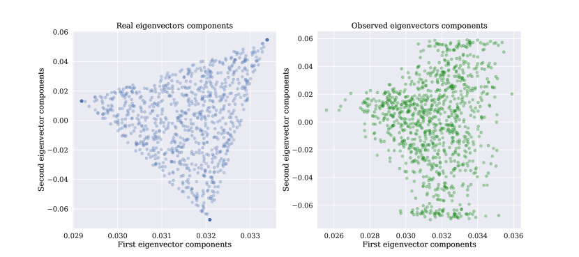
Figure 1: First and second components of rows of matrices $\mathbf{U}$, $\widehat{\mathbf{U}}$ in the case of $K$ being equal to $3$.

Algorithm 1 SPA (Mizutani, 2016)

1:Matrix $\mathbf{V}\in\mathbb{R}^{n\times K}$ and integer $r\leqslant K$

2:Set of indices $J\subset[n]$

3:Set $\mathbf{S}^{0}=\mathbf{V}$, $J_{0}=\varnothing$

4:for $t=1\ldots r$ do

5:     Find $j_{t}=\arg\min_{i\in[n]}\|\mathbf{S}^{t-1}_{i}\|$

6:     Project rows of $\mathbf{S}^{t-1}$ on the plane orthogonal to $\mathbf{S}^{t-1}_{j_{t}}$:

$$\mathbf{S}^{t}=\mathbf{S}^{t-1}\left(\mathbf{I}_{K}-\frac{\mathbf{S}^{t-1}_{j_{t}}(\mathbf{S}^{t-1}_{j_{t}})^{\mathrm{T}}}{\|\mathbf{S}^{t-1}_{j_{t}}\|^{2}_{2}}\right).$$

7:     Add $j_{t}$ to the set $J$: $J_{t}=J_{t-1}\cup\{j_{t}\}$.

8:end for

9:return $J_{t}$

The most natural way to estimate $\mathbf{U}$ and $\mathbf{L}$ is to use a $K$-eigenvalue decomposition of the adjacency matrix $\mathbf{A}\simeq\widehat{\mathbf{U}}\widehat{\mathbf{L}}\widehat{\mathbf{U}}^{\mathrm{T}}$, where columns of $\widehat{\mathbf{U}}$ are first $K$ eigenvectors of $\mathbf{A}$ and $\widehat{\mathbf{L}}$ is the diagonal matrix of eigenvalues. The rows of matrix $\widehat{\mathbf{U}}$ lie in a perturbed version of the simplex corresponding to matrix $\mathbf{U}$, see illustration on Figure 1. To find vertices of the perturbed simplex, we run Successive Projections Algorithm (SPA), see Algorithm 1. The resulting SPOC algorithm is given in Algorithm 2.

Algorithm 2 SPOC

1:Adjacency matrix $\mathbf{A}$, number of communities $K$.

2:Estimators $\widehat{\boldsymbol{\mathrm{\Theta}}}$, $\widehat{\mathbf{B}}$

3:Get the rank-$K$ eigenvalue decomposition $\mathbf{A}\simeq\widehat{\mathbf{U}}\widehat{\mathbf{L}}\widehat{\mathbf{U}}^{\mathrm{T}}$

4:Run SPA algorithm with input $(\widehat{\mathbf{U}},K)$, which outputs the set of indices $J$ of cardinality $K$

5:$\widehat{\mathbf{F}}=\widehat{\mathbf{U}}[J,:]$

6:$\widehat{\mathbf{B}}=\widehat{\mathbf{F}}\widehat{\mathbf{L}}\widehat{\mathbf{F}}^{\mathrm{T}}$

7:$\widehat{\boldsymbol{\mathrm{\Theta}}}=\widehat{\mathbf{U}}\widehat{\mathbf{F}}^{-1}$

However, the SPOC-based estimator $\widehat{\mathbf{B}}$ does not allow for obtaining the optimal rate of estimation (4), only achieving the suboptimal one (1). The nature of the problem is in the SPA algorithm whose error is driven by the properties of rows of matrix $\widehat{\mathbf{U}}$ that might be too noisy. In what follows, we will provide a noise reduction procedure for it.

2.2 Denoising via averaging

Algorithm 3 Averaging procedure

1:Matrix of eigenvectors $\widehat{\mathbf{U}}$, diagonal matrix of eigenvalues $\widehat{\mathbf{L}}$, estimator $\tilde{\mathbf{L}}$, number of communities $K$, threshold $t_{n}$, indices $J$, regularization parameter $a$

2:$\widehat{\mathbf{F}}$ — an estimator of the matrix $\mathbf{F}$.

3:Calculate an estimator ${\widehat{\mathbf{W}}}=\mathbf{A}-\widehat{\mathbf{U}}\tilde{\mathbf{L}}\widehat{\mathbf{U}}^{\mathrm{T}}$.

4:for $j$ in $J$ do

5:     for $j^{\prime}=1$ to $n$ do

6:         Calculate covariance matrix estimator

$${\widehat{\mathbf{\Sigma}}}(j,j^{\prime})=\tilde{\mathbf{L}}^{-1}\widehat{\mathbf{U}}^{\mathrm{T}}\left(\operatorname{diag}({\widehat{\mathbf{W}}}_{j}^{2}+{\widehat{\mathbf{W}}}_{j^{\prime}}^{2})-{\widehat{\mathbf{W}}}_{jj^{\prime}}^{2}(\mathbf{e}_{j}\mathbf{e}_{j^{\prime}}^{\mathrm{T}}+\mathbf{e}_{j^{\prime}}\mathbf{e}_{j}^{\mathrm{T}})\right)\widehat{\mathbf{U}}\tilde{\mathbf{L}}^{-1},$$ (5)

   where the square is an element-wise operation.

7:         Calculate statistic ${\widehat{T}}_{jj^{\prime}}^{a}=(\widehat{\mathbf{U}}_{j}-\widehat{\mathbf{U}}_{j^{\prime}})\left({\widehat{\mathbf{\Sigma}}}(j,j^{\prime})+a\mathbf{I}\right)^{-1}(\widehat{\mathbf{U}}_{j}-\widehat{\mathbf{U}}_{j^{\prime}})^{\mathrm{T}}$.

8:     end for

9:     Select nodes $\mathcal{I}_{j}=\{j^{\prime}\in[n]\mid T_{jj^{\prime}}<t_{n}\}$

10:     Reduce bias in estimation of $\mathbf{U}:$

$$\mathbf{D} =\operatorname{diag}\left(\sum_{t=1}^{n}\mathbf{A}_{it}\right)_{i=1}^{n},$$ (6)

$$\tilde{\mathbf{U}}_{ik} =\widehat{\mathbf{U}}_{ik}\left(1-\frac{\mathbf{D}_{ii}-3/2\sum_{j=1}^{n}\mathbf{D}_{jj}\widehat{\mathbf{U}}_{jk}^{2}}{\widehat{\mathbf{L}}^{2}_{k^{\prime}k^{\prime}}}\right)-\sum_{k^{\prime}\in[K]\setminus\{k\}}\frac{\tilde{\mathbf{L}}_{k^{\prime}k^{\prime}}\cdot\widehat{\mathbf{U}}_{ik^{\prime}}}{\tilde{\mathbf{L}}_{k^{\prime}k^{\prime}}-\widehat{\mathbf{L}}_{kk}}\cdot\sum_{j=1}^{n}\frac{\mathbf{D}_{jj}\widehat{\mathbf{U}}_{jk^{\prime}}\widehat{\mathbf{U}}_{jk}}{\widehat{\mathbf{L}}_{kk}^{2}}.$$ (7)

11:     Average rows of matrix $\tilde{\mathbf{U}}$ over the set $\mathcal{I}_{j}$ and write result into vector ${\widehat{\mathbf{f}}}(j)$:

$${\widehat{\mathbf{f}}}^{\mathrm{T}}(j)=\frac{1}{|\mathcal{I}_{j}|}\sum_{j^{\prime}\in\mathcal{I}_{j}}\tilde{\mathbf{U}}_{j^{\prime}}.$$ (8)

12:end for

13:Stack together row-vectors ${\widehat{\mathbf{f}}}^{\mathrm{T}}(j)$ into matrix $\widehat{\mathbf{F}}$:

$$\widehat{\mathbf{F}}=\left({\widehat{\mathbf{f}}}^{\mathrm{T}}(j)\right)_{j\in J}.$$ (9)

14:Return matrix $\widehat{\mathbf{F}}$

The most common denoising tool is averaging because it decreases the variance of i.i.d. variables by $\sqrt{N}$ where $N$ is a sample size. In this work, our key idea is to reduce the error rate of the estimation of the matrix $\mathbf{F}$ by $\sqrt{n}$ times through averaging $\Theta(n)$ rows of $\widehat{\mathbf{U}}$. The key contribution of this work is in establishing the procedure for finding the rows similar to the rows of $\mathbf{F}$ and dealing with their weak dependence on each other.

We call the $i$-th node “pure” if the corresponding row $\boldsymbol{\mathrm{\Theta}}_{i}$ of the matrix $\boldsymbol{\mathrm{\Theta}}$ consists only of zeros except for one particular entry, equal to $1$. Thus, for the pure node $\mathbf{U}_{i}=\mathbf{F}_{k}$ for some $k\in[K]$. If we find many pure nodes and average corresponding rows of $\widehat{\mathbf{U}}$, we can get a better estimator of rows of $\mathbf{F}$ and, consequently, matrix $\mathbf{B}$.

To find pure nodes, we employ the following strategy. In the first step, we run the SPA algorithm and obtain one vertex per community. Below, we prove under some conditions that SPA chooses “almost” pure nodes with high probability. In the second step, we detect the nodes which are “similar” to the ones selected by SPA and use the resulting pure nodes set for averaging. The complete averaging procedure is given in Algorithm 3, while we discuss its particular steps below.

The choice of similarity measure for detection on similar nodes is crucial for our approach. Fan et al. (2022) provide a statistical test for equality of node membership vectors $\boldsymbol{\mathrm{\Theta}}_{i}$ and $\boldsymbol{\mathrm{\Theta}}_{j}$ based on the statistic $T_{ij}$. This statistic is closely connected to the displace matrix

$$\mathbf{W}=\mathbf{A}-\mathbf{P}$$

and covariance matrix $\mathbf{\Sigma}(i,j)$ of the vector $(\mathbf{W}_{i}-\mathbf{W}_{j})\mathbf{U}\mathbf{L}^{-1}$:

$$\mathbf{\Sigma}(i,j)=\mathbb{E}\bigl{[}\mathbf{L}^{-1}\mathbf{U}^{\mathrm{T}}(\mathbf{W}_{i}-\mathbf{W}_{j})^{\mathrm{T}}(\mathbf{W}_{i}-\mathbf{W}_{j})\mathbf{U}\mathbf{L}^{-1}\bigr{]}.$$

Thus, the test statistic $T_{ij}$ is given by

$$T_{ij}=(\widehat{\mathbf{U}}_{i}-\widehat{\mathbf{U}}_{j})\mathbf{\Sigma}(i,j)^{-1}(\widehat{\mathbf{U}}_{i}-\widehat{\mathbf{U}}_{j})^{\mathrm{T}}.$$

However, we do not observe the matrix $\mathbf{\Sigma}(i,j)$. Instead, we use its plug-in estimator ${\widehat{\mathbf{\Sigma}}}(i,j)$ which is described below in Algorithm 3, see equation (5). Thus, the resulting test statistic is given by

$${\widehat{T}}_{ij}=(\widehat{\mathbf{U}}_{i}-\widehat{\mathbf{U}}_{j}){\widehat{\mathbf{\Sigma}}}(i,j)^{-1}(\widehat{\mathbf{U}}_{i}-\widehat{\mathbf{U}}_{j})^{\mathrm{T}}.$$ (10)

Fan et al. (2022) prove that under some conditions $T_{ij}$ and ${\widehat{T}}_{ij}$ both converge to non-central chi-squared distribution with $K$ degrees of freedom and center

$$\bar{T}_{ij}=(\mathbf{U}_{i}-\mathbf{U}_{j})\mathbf{\Sigma}(i,j)^{-1}(\mathbf{U}_{i}-\mathbf{U}_{j})^{\mathrm{T}}.$$ (11)

Thus, ${\widehat{T}}_{ij}$ can be considered as a measure of closeness for two nodes. For each node $i$ we can define its neighborhood $\mathcal{I}_{i}$ as all nodes $j$ such that ${\widehat{T}}_{ij}$ is less than some threshold $t_{n}$: $\mathcal{I}_{i}=\{j\in[n]\mid{\widehat{T}}_{ij}<t_{n}\}$.

To evaluate $\bar{T}_{ij}$, one needs to invert the matrix $\mathbf{\Sigma}(i,j)$. However, matrix $\mathbf{\Sigma}(i,j)$ can be degenerate in the general case. Nevertheless, one can specify some conditions on matrix $\mathbf{B}$ to ensure it is well-conditioned. To illustrate it, let us consider the following proposition.

Proposition 1.

Let Conditions 1-4, defined below, hold. Assume additionally that entries of the matrix $\mathbf{B}$ are bounded away from 0 and 1. Then there exist constants $C_{1},C_{2}$ such that for large enough $n$ it holds

$$\frac{C_{1}}{n^{2}\rho}\leqslant\lambda_{\min}(\mathbf{\Sigma}(i,j))\leqslant\lambda_{\max}(\mathbf{\Sigma}(i,j))\leqslant\frac{C_{2}}{n^{2}\rho}$$

for any nodes $i$ and $j$.

However, the condition on the entries of the community matrix above might be too strong, while we only need concentration bounds on ${\widehat{T}}_{ij}$. To not limit ourselves to matrices $\mathbf{B}$ with no zero entries, we consider a regularized version of ${\widehat{T}}_{ij}$:

$${\widehat{T}}_{ij}^{a}=(\widehat{\mathbf{U}}_{i}-\widehat{\mathbf{U}}_{j})\left({\widehat{\mathbf{\Sigma}}}(i,j)+a\mathbf{I}\right)^{-1}(\widehat{\mathbf{U}}_{i}-\widehat{\mathbf{U}}_{j})^{\mathrm{T}}$$

for some $a>0$. When $a=\Theta(n^{-2}\rho^{-1})$, the statistic ${\widehat{T}}^{a}_{ij}$ concentrates around

$$\bar{T}^{a}_{ij}=(\mathbf{U}_{i}-\mathbf{U}_{j})\left(\mathbf{\Sigma}(i,j)+a\mathbf{I}\right)^{-1}(\mathbf{U}_{i}-\mathbf{U}_{j})^{\mathrm{T}}.$$

Practically, if ${\widehat{\mathbf{\Sigma}}}(i,j)$ is well-conditioned, one can use the statistic ${\widehat{T}}_{ij}$ without any regularization. In other words, all of our results still hold if $a=0$ and $\lambda_{\min}\bigl{(}\mathbf{\Sigma}(i,j)\bigr{)}\geqslant Cn^{-2}\rho^{-1}$ for all $i,j$. But to not impose additional assumptions on either matrix $\mathbf{B}$ or $\boldsymbol{\mathrm{\Theta}}$, in what follows we will use ${\widehat{T}}^{a}_{ij}$ with $a=\Theta(n^{-2}\rho^{-1})$.

2.3 Estimation of eigenvalues and eigenvectors

It turns out that the eigenvalues $\widehat{\mathbf{L}}$ and eigenvectors $\widehat{\mathbf{U}}$ of $\mathbf{A}$ are not optimal estimators of $\mathbf{L},\mathbf{U}$ respectively. The asymptotic expansion of $\mathbf{U}$ described in Lemma 6 suggests a new estimator $\tilde{\mathbf{U}}$ that suppresses some high-order terms in the expansion. For the exact formula, see equation (7) in Algorithm 3. Similarly, a better estimator $\tilde{\mathbf{L}}$ of eigenvalues exists; see equation (12) in Algorithm 4.

Proposed estimators admit better asymptotic properties than $\widehat{\mathbf{L}}$ and $\widehat{\mathbf{U}}$, see Lemma 9 and 16 below. In particular, it allows us to achieve the convergence rate (4) instead of $1/n$.

Algorithm 4 SPOC++

1:Adjacency matrix $\mathbf{A}$, threshold $t_{n}$, regularization parameter $a$

2:Estimators $\widehat{\boldsymbol{\mathrm{\Theta}}}$, $\widehat{\mathbf{B}}$

3:Estimate rank with ${\widehat{K}}=\max\bigl{\{}j\mid\lambda_{j}(\mathbf{A})\geqslant 2\max_{i}\sqrt{\sum\nolimits_{t=1}^{n}\mathbf{A}_{it}\log^{2}n}\bigr{\}}$

4:Get the rank-${\widehat{K}}$ eigenvalue decomposition of $\mathbf{A}\simeq\widehat{\mathbf{U}}\widehat{\mathbf{L}}\widehat{\mathbf{U}}^{\mathrm{T}}$

5:Run SPA algorithm with input $(\widehat{\mathbf{U}},{\widehat{K}})$, which outputs the set of indices $J$ of cardinality $K$

6:Calculate the estimator of the eigenvalues’ matrix:

$$\tilde{\mathbf{L}}_{kk}=\left[\frac{1}{\widehat{\mathbf{L}}_{kk}}+\frac{\sum_{i=1}^{n}\widehat{\mathbf{U}}_{ik}^{2}\cdot\sum_{t=1}^{n}\mathbf{A}_{it}}{\widehat{\mathbf{L}}_{kk}^{3}}\right]^{-1}.$$ (12)

7:$\widehat{\mathbf{F}}=\operatorname{avg}(\widehat{\mathbf{U}},\widehat{\mathbf{L}},\tilde{\mathbf{L}},t_{n},J,a)$, where $\operatorname{avg}$ is the averaging procedure described in Algorithm 3.

8:$\widehat{\mathbf{B}}=\widehat{\mathbf{F}}\tilde{\mathbf{L}}\widehat{\mathbf{F}}^{\mathrm{T}}$

9:$\widehat{\boldsymbol{\mathrm{\Theta}}}=\widehat{\mathbf{U}}\widehat{\mathbf{F}}^{-1}$

2.4 Estimation of $K$

In the previous sections, we assumed that the number of communities $K$ is known. However, in practical scenarios, this assumption often does not hold. This section presents an approach to estimating the number of communities.

The idea is to find the efficient rank of the matrix $\mathbf{A}$. Due to Weyl’s inequality $|\lambda_{j}(\mathbf{A})-\lambda_{j}(\mathbf{P})|\leqslant\|\mathbf{A}-\mathbf{P}\|$. Efficiently bounding the norm $\|\mathbf{A}-\mathbf{P}\|$, we obtain that it much less than $2\max_{i\in[n]}\sqrt{\sum_{t=1}^{n}\mathbf{A}_{it}\log^{2}n}$. However, in its turn, $2\max_{i\in[n]}\sqrt{\sum_{t=1}^{n}\mathbf{A}_{it}\log^{2}n}\ll\lambda_{K}(\mathbf{P})$. Thus, we suggest the following estimator:

$${\widehat{K}}=\max\left\{j\mid\lambda_{j}(\mathbf{A})\geqslant 2\max_{i\in[n]}\sqrt{\sum\nolimits_{t=1}^{n}\mathbf{A}_{it}\log^{2}n}\right\}.$$

In what follows, we prove that it coincides with $K$ with high probability if $n$ is large enough; see Section B.4 of Appendix for details.

2.5 Resulting SPOC++ algorithm

Combining ideas from previous sections, we split our algorithm into two procedures:
Averaging Procedure (Algorithm 3) and the resulting SPOC++ method (Algorithm 4).

However, the critical question remains: how to select the threshold $t_{n}$? In our theoretical analysis (see Theorem 2 below), we demonstrate that by setting $t_{n}$ to be logarithmic in $n$, SPOC++ can recover the matrix $\mathbf{B}$ with a high probability and up to the desired error level. However, for practical purposes, we recommend defining the threshold just considering the distribution of the statistics ${\widehat{T}}_{i_{k}j}^{a}$ for different $j$, where $i_{k}$ is an index chosen by Algorithm 1; see Section 4.1 for details.

3 Provable guarantees

3.1 Sketch of the proof of consistency

We will need several conditions to be satisfied to obtain optimal convergence rates. The most important one is to have many nodes placed near the vertices of the simplex. We will give the exact conditions and statements below, but first, discuss the key steps that allow us to achieve the result. They are listed below.

Step 1. Asymptotics of $\widehat{\mathbf{U}}_{ik}$. First, using results of (Fan et al., 2020), we obtain the asymptotic expansion of $\widehat{\mathbf{U}}_{ik}$. We show that up to a residual term of order $\sqrt{\frac{\log n}{n^{3}\rho}}$ we have

$$\widehat{\mathbf{U}}_{ik} \approx\mathbf{U}_{ik}+\frac{\mathbf{e}_{i}^{\mathrm{T}}\mathbf{W}\mathbf{u}_{k}}{t_{k}}+\frac{\mathbf{e}_{i}^{\mathrm{T}}\mathbf{W}^{2}\mathbf{u}_{k}}{t_{k}^{2}}-\frac{3}{2}\cdot\mathbf{U}_{ik}\frac{\mathbf{u}_{k}^{\mathrm{T}}\mathbb{E}\mathbf{W}^{2}\mathbf{u}_{k}}{t_{k}^{2}}+\frac{1}{t_{k}^{2}}\sum_{k^{\prime}\in[K]\setminus\{k\}}\frac{\lambda_{k^{\prime}}\mathbf{U}_{ik^{\prime}}}{\lambda_{k^{\prime}}-t_{k}}\cdot\mathbf{u}_{k^{\prime}}^{\mathrm{T}}\mathbb{E}\mathbf{W}^{2}\mathbf{u}_{k},$$

where $t_{k}\approx\lambda_{k}(\mathbf{P})$. Matrices $\mathbb{E}\mathbf{W}^{2}$ and $\mathbf{W}^{2}$ can be efficiently estimated by diagonal matrix $\mathbf{D}=\operatorname{diag}\left(\sum_{t=1}^{n}\mathbf{A}_{it}\right)_{i=1}^{n}$, see also equation (6) in Algorithm 3. Thus, we proceed with plug-in estimation of the second-order terms and obtain the estimator $\tilde{\mathbf{U}}$ defined in (7). Most importantly, the term linear in $\mathbf{W}$ can be suppressed using averaging.

Step 2. Approximating the set of pure nodes. We show that the difference $|{\widehat{T}}^{a}_{ij}-\bar{T}^{a}_{ij}|$ can be efficiently bounded by sum of two terms: one depends on the difference $\|\boldsymbol{\mathrm{\Theta}}_{i}-\boldsymbol{\mathrm{\Theta}}_{j}\|_{2}$ and the other is at most logarithmic. If $i_{k}$ is an index chosen by SPA and $j\in\mathcal{P}_{k}$, then $\bar{T}_{i_{k}j}^{a}$ is small. Thus, logarithmic threshold $t_{n}$ will ensure that for all $j\in\mathcal{P}_{k}$ we have ${\widehat{T}}^{a}_{i_{k}j}\leqslant t_{n}$. Next, Condition 5 implies that there are a few non-pure nodes in the set $\{j\mid{\widehat{T}}^{a}_{i_{k}j}\leqslant t_{n}\}$.

Step 3. Averaging. Finally, we show that redundant terms in the asymptotic expansion of $\tilde{\mathbf{U}}_{i}-\mathbf{U}_{i}$ vanish after averaging, and it delivers an appropriate estimator of the simplex vertices. After that, we can obtain a good estimator of the matrix $\mathbf{B}$.

3.2 Main result

In order to perform theoretical analysis, we state some conditions. Most of these conditions are not restrictive, and below we discuss their limitations, if any.

Condition 1.

Singular values of the matrix $\bar{\mathbf{B}}$ are bounded away from 0.

The full rank condition is essential as, otherwise, one loses the identifiability of communities (Mao et al., 2017).

Condition 2.

There is some constant $c$ such that $0\leqslant c<1/3$ and $\rho>n^{-c}$.

Parameter $\rho$ is responsible for the sparsity of the resulting graph. The most general results on statistical properties of random graphs require $\rho n\to\infty$ as $n\to\infty$ (Tang et al., 2022). In this work, we require a stronger condition to achieve the relatively strong statements we aim at. We think this condition can be relaxed though it would most likely need a proof technique substantially different from ours.

Next, we demand the technical condition for the probability matrix $\mathbf{P}$.

Condition 3.

There exists some constant $c_{0}>0$ such that

$$\min\left\{\frac{|\lambda_{i}(\mathbf{P})|}{|\lambda_{j}(\mathbf{P})|}\mid 1\leqslant i<j\leqslant K,\lambda_{i}(\mathbf{P})\neq\lambda_{j}(\mathbf{P})\right\}\geqslant 1+c_{0}.$$

In addition, we have

$$\max_{j}\sum_{i=1}^{n}\mathbf{P}_{ij}(1-\mathbf{P}_{ij})\to\infty$$ (13)

as $n$ tends to $\infty$.

This condition is required because of the method to obtain asymptotics of eigenvectors of $\mathbf{A}$. The idea is to apply the Cauchy residue theorem to the resolvent. Let ${\widehat{\mathbf{u}}}_{k}$ be the $k$-th eigenvector of $\mathbf{A}$ and $\mathbf{u}_{k}$ be the $k$-th eigenvector of $\mathbf{P}$. Let $\mathcal{C}_{k}$ be a contour in the complex plane that contains both $\lambda_{k}(\mathbf{P})$ and $\lambda_{k}(\mathbf{A})$. If no other eigenvalues are contained in $\mathcal{C}_{k}$ then

$$\oint_{\mathcal{C}_{k}}\frac{\mathbf{x}^{\mathrm{T}}{\widehat{\mathbf{u}}}_{k}{\widehat{\mathbf{u}}}_{k}^{\mathrm{T}}\mathbf{y}}{\lambda_{k}(\mathbf{A})-z}dz=\oint_{\mathcal{C}_{k}}\mathbf{x}^{\mathrm{T}}(\mathbf{A}-z\mathbf{I})^{-1}\mathbf{y}dz=\oint_{\mathcal{C}_{k}}\mathbf{x}^{\mathrm{T}}\left(\sum_{k=1}^{K}\lambda_{k}(\mathbf{P})\mathbf{u}_{k}\mathbf{u}_{k}^{\mathrm{T}}+\mathbf{W}-z\mathbf{I}\right)^{-1}\mathbf{y}dz$$

for any vectors $\mathbf{x},\mathbf{y}$. The leftmost side is simplified by calculating the residue at $\lambda_{k}(\mathbf{A})$, and the rightmost side is analyzed via Sherman–Morrison–Woodbury formula. For the example of obtained asymptotics, see Lemma 6.

The second part of Condition 3 can be omitted if $\rho<1$ or there exist $k,k^{\prime}\in[K]$ such that $\mathbf{B}_{kk^{\prime}}$ is bounded away from $0$ and 1, since (13) is granted by Conditions 1-2 and 4 in this case. However, we decided not to impose additional assumptions and left this condition as proposed by Fan et al. (2022).

Next, we call the $i$-th node in our graph pure if $\boldsymbol{\mathrm{\Theta}}_{i}$ has $1$ in some position and $0$ in others. We also denote this non-zero position by $\operatorname{cl}(i)$ and the set of pure nodes by $\mathcal{P}$. Moreover, we define $\mathcal{P}_{k}=\{i\in\mathcal{P}\mid\operatorname{cl}(i)=k\}$. Thus, $\mathcal{P}_{k}$ is a set of nodes completely belonging to the $k$-th community. It leads us to the following conditions.

Condition 4.

Cardinality of $\mathcal{P}_{k}$ has an asymptotic order of $n$ for all $k=1,\dots,K$. More formally,

$$|\mathcal{P}_{k}|=\Theta(n).$$

Condition 5.

Fix $\eta\geqslant 1$. For any community index $k$, $\delta>0$ and $n>n_{0}(\delta)$ there exists $C_{\delta}$ such that

$$\sum_{j\not\in\mathcal{P}_{k}}{\operatorname{I}\left\{\|\boldsymbol{\mathrm{\Theta}}_{j}-\mathbf{e}_{k}\|_{2}\leqslant\delta\sqrt{\frac{\log n}{n\rho}}\right\}}\leqslant C_{\delta}\log^{\eta}n,$$ (14)

where $\mathbf{e}_{k}$ is the $k$-th standard basis vector in $\mathbb{R}^{K}$.

Condition 4 is essential as it requires that all the communities have asymptotically significant mass. As discussed in Section 2.2, we employ row averaging on the eigenmatrix $\widehat{\mathbf{U}}$ to mitigate noise, specifically focusing on rows corresponding to pure nodes. This averaging process effectively reduces noise by a factor of $\sqrt{n}$. While this condition is not commonly encountered in the context of MMSB, it covers an important intermediate case bridging the gap between the Stochastic Block Model and the Mixed-Membership Stochastic Block Model. If this condition is not satisfied, we suppose it is possible to obtain a higher minimax lower bound than the one provided by Theorem 3.

Condition 5 can be naturally fulfilled if non-pure $\boldsymbol{\mathrm{\Theta}}_{j}$ are sampled from the Dirichlet distribution. Indeed, the number of $\boldsymbol{\mathrm{\Theta}}_{j}$ in a ball of radius $\sqrt{\frac{\log n}{n\rho}}$ is proportional to $n\cdot\left[\frac{\log n}{n\rho}\right]^{\frac{K-1}{2}}$. For example, if $\rho=\Theta(1)$ and $K\geqslant 3$, then we have

$$\sum_{j\not\in\mathcal{P}_{k}}{\operatorname{I}\left\{\|\boldsymbol{\mathrm{\Theta}}_{j}-\mathbf{e}_{k}\|_{2}\leqslant\delta\sqrt{\frac{\log n}{n\rho}}\right\}}\sim C_{\delta}n\cdot\left[\frac{\log n}{n\rho}\right]^{\frac{K-1}{2}}\lesssim C_{\delta}\log^{(K-1)/2}n$$

with high probability. In this case, one can take $\eta=(K-1)/2$.

One may prove the above by bounding the sum of Bernoulli random variables on the left-hand side using the Bernstein inequality.

These conditions allow us to state the main result of this work.

Theorem 2.

Suppose that $a=\Theta(n^{-2}\rho^{-1})$. Under Conditions 1-5, for each positive $\varepsilon$ there are constants $C_{t},C_{\mathbf{B}}$ depending on $\varepsilon,K$ such that if we apply Algorithm 4 with

$$t_{n}=C_{t}\log n,$$ (15)

then there is $n_{0}$ such that for all $n>n_{0}$ the following inequality holds:

$$\mathbb{P}\left(\min_{\mathbf{\Pi}\in\mathbb{S}_{K}}\|{\widehat{\mathbf{B}}}-\mathbf{\Pi}\mathbf{B}\mathbf{\Pi}^{\mathrm{T}}\|_{\mathrm{F}}\geqslant\frac{C_{\mathbf{B}}\sqrt{\rho}\log^{\eta}n}{n}\right)\leqslant n^{-\varepsilon}.$$

The theorem demands $a=\Theta(n^{-2}\rho^{-1})$, but the sparsity parameter $\rho$ is not observed in practice. We suppose that the most convenient choice is $a=0$, see discussion in Section 2.2. However, if one need to construct a quantity of order $n^{-2}\rho^{-1}$, one can choose $\bigl{(}n\lambda_{1}(\mathbf{A})\bigr{)}^{-1}$, see Lemma 25.

3.3 Proof of Theorem 2

Assume that $K$ is known. Given $\varepsilon$, choose $t_{n}=C(\varepsilon)\log n$ such that the event

$$\|{\widehat{\mathbf{F}}}-\mathbf{F}\mathbf{\Pi}_{\mathbf{F}}\|_{\mathrm{F}}\leqslant\frac{C_{\mathbf{F}}\log^{\eta}n}{n\sqrt{n\rho}}$$ (16)

has probability at least $1-n^{-\varepsilon}/3$ for some constant $C_{\mathbf{F}}$ and permutation matrix $\mathbf{\Pi}_{\mathbf{F}}$. Such $t_{n}$ exists due to Lemma 9. WLOG, we assume that the minimum in (16) is attained when $\mathbf{\Pi}_{\mathbf{F}}=\mathbf{I}$, since changing order of communities does not change the model. Meanwhile, due to Lemma 16:

$$\tilde{\mathbf{L}}_{kk}=\mathbf{L}_{kk}+O_{\ell}(\sqrt{\rho\log n}).$$

Thus, we have

$$\max_{k}|\tilde{\mathbf{L}}_{kk}-\mathbf{L}_{kk}|\leqslant C_{\mathbf{L}}\sqrt{\rho\log n}$$

with probability $1-n^{-\varepsilon}/3$. Hence, we obtain

$$\|\mathbf{B}-{\widehat{\mathbf{B}}}\|_{\mathrm{F}}\leqslant\|\mathbf{F}-{\widehat{\mathbf{F}}}\|\|\mathbf{L}\|\|\mathbf{F}\|_{\mathrm{F}}+\|{\widehat{\mathbf{F}}}\|\|\mathbf{L}-\tilde{\mathbf{L}}\|\|\mathbf{F}\|_{\mathrm{F}}+\|{\widehat{\mathbf{F}}}\|\|\tilde{\mathbf{L}}\|\|\mathbf{F}-{\widehat{\mathbf{F}}}\|_{\mathrm{F}}\\ =O\left(\frac{\sqrt{\rho}}{n}\cdot\log^{\eta}n\right),$$

where we use $\|\mathbf{F}\|_{\mathrm{F}}=O(n^{-1/2})$ and $\|\mathbf{L}\|=O(n\rho)$ from Lemmas 24 and 25.

Before we supposed that $K$ is known. Now consider the case when it does not hold. Due to Lemma 10, we have ${\widehat{K}}=K$ with probability $1-n^{-\varepsilon}/3$ for large enough $n$. It implies that the bound (3.3) also holds for the estimator based on ${\widehat{K}}$ with probability $1-n^{-\varepsilon}$.

3.4 Lower bound

In this section, we show that Theorem 2 is optimal under Conditions 1-5. Precisely, we state the following.

Theorem 3.

If $n>n_{0}$ for some $n_{0}$ that may depend on $K$, then there exist a matrix $\boldsymbol{\mathrm{\Theta}}_{0}$ and a set of symmetric matrices $\mathcal{B}\subset[0,1]^{K\times K}$ such that

1. for each matrix $\bar{\mathbf{B}}\in\mathcal{B}$, its singular values are at least $1/8$,

2. for each $k\in[K-1]$ and $\bar{\mathbf{B}}\in\mathcal{B}$, we have $\sigma_{k}(\mathbf{P})/\sigma_{k+1}(\mathbf{P})>1+c_{0}$, where $c_{0}=0.2$ and $\mathbf{P}=\boldsymbol{\mathrm{\Theta}}_{0}\bar{\mathbf{B}}\boldsymbol{\mathrm{\Theta}}_{0}^{\mathrm{T}}$, and, additionally,

   $$\max_{j}\sum_{i=1}^{n}\mathbf{P}_{ij}(1-\mathbf{P}_{ij})\geqslant\frac{n\rho}{16},$$

3. each set $|\mathcal{P}_{k}|$, $k\in[K]$, has cardinality at least $\left(1-2^{-(K+5)}\right)2^{-K}n$,

4. for each $k$, we have

   $$\sum_{j\not\in\mathcal{P}_{k}}{\operatorname{I}\left\{\|\boldsymbol{\mathrm{\Theta}}_{j}-\mathbf{e}_{k}\|_{2}\leqslant\delta\sqrt{\frac{\log n}{n\rho}}\right\}}=0,$$

   provided $n\rho>\delta^{2}\left(1-K^{-2}\right)\log n$,

and

$$\inf_{{\widehat{\mathbf{B}}}}\sup_{\bar{\mathbf{B}}\in\mathcal{B}}\mathbb{P}\left(\min_{\mathbf{\Pi}\in\mathbb{S}_{K}}\|\rho\bar{\mathbf{B}}-\mathbf{\Pi}{\widehat{\mathbf{B}}}\mathbf{\Pi}^{\mathrm{T}}\|_{\mathrm{F}}\geqslant\frac{K^{2}\sqrt{\rho}}{1152\cdot n}\right)\geqslant\frac{1}{4e^{3.2}}$$

for any $\rho>n^{-1/3}$.

The proof is similar to that of (2). The main difference is that we consider the minimum over the set of permutation matrices.

One can see that Condition 1 is satisfied by property (i), Condition 2 is satisfied since we guarantee the conclusion of Theorem 3 for any $\rho>n^{-1/3}$, Condition 3 is satisfied by property (ii), Condition 4 is satisfied by property (iii), and Condition 5 is satisfied by property (iv). Thus, the estimator defined by Algorithm 4 is indeed optimal up to the dependence on $K$.

4 Numerical experiments

4.1 How to choose an appropriate threshold?

In the considered experiments, we fix $K$ equal to $3$ and assume that $\mathbf{B}$ is well-conditioned. Empirically we show that well-conditioning is vital to achieving a high probability of choosing pure nodes with SPA (see Figure 2).

The crucial question in practice for the SPOC++ algorithm is the choice of the threshold. Theoretically, we have established that $t=C\log n$ gives the right threshold to achieve good estimation quality. In practice, there is a simple way to choose the appropriate threshold for nodes $i_{1},\ldots,i_{K}$ chosen by SPA. For each $i_{k}$, it is necessary to plot distribution of ${\widehat{T}}_{i_{k}j}$ over $j$. Thus, if the averaging procedure improves the results of SPOC, then there is a corresponding plateau on the plot (see Figure 3).

Besides, our experiments show that for small $K$, $t_{n}=2\log n$ is good enough if nodes are generated to satisfy Conditions 4 and 5. This choice corresponds well to the theory developed in this paper.

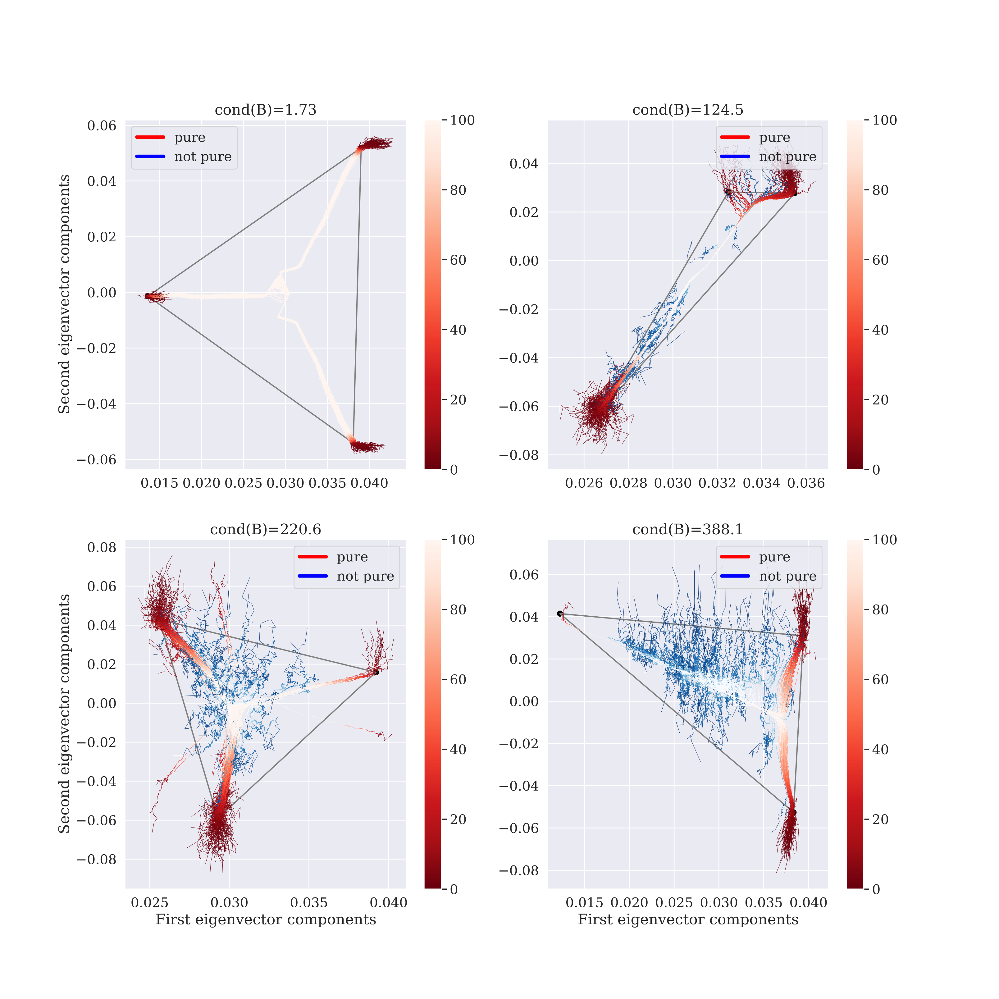
Figure 2: Varying $t_{n}$, we draw curves ${\widehat{\mathbf{F}}}_{k}(t_{n}),k\in[K],$ projected on the two first coordinates, where ${\widehat{\mathbf{F}}}_{k}$ is defined in Algorithm 3. The intensity of a color corresponds to the value of $t_{n}$. A curve is red if SPA chooses a pure node, otherwise, the curve is blue. We consider four different matrices $\mathbf{B}$, each has different conditional number. For each matrix $\mathbf{B}$, we construct one matrix $\mathbf{P}$, and for this matrix $\mathbf{P}$, we generate 100 matrices $\mathbf{A}$. We choose $n=1000$ and $|\mathcal{P}_{k}|/n=0.07$, $k\in[K]$. Non-pure membership vectors $\bm{\theta}_{i}$ were sampled from $Dirichlet(1,1,1)$.

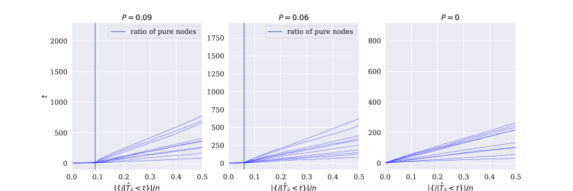
Figure 3: The distribution of ${\widehat{T}}_{i_{1}j}$ over $j$ where $i_{1}$ is the first choice of SPA. Here $P=\frac{|\mathcal{P}_{k}|}{n}$ which is equal for every $k$ in our partial case. It is painted on the plot by the vertical line. Different blue curves are related to different $n$.

4.2 Illustration of theoretical results

We run two experiments to illustrate our theoretical studies. First, we check the dependence of the estimation error on the number of vertices $n$. Second, we study how the sparsity parameter $\rho$ influences the error.

For the first experiment, we provide the following experimental setup. The number of clusters is chosen equal to $3$, and for each $n\in\{500,1000,1500,\ldots,5000\}$ we generate a matrix $\boldsymbol{\mathrm{\Theta}}$, where the fractions of pure nodes are $\frac{|\mathcal{P}_{k}|}{n}=0.09$ and other (not pure) node community memberships are distributed in simplex according to $Dirichlet(1,1,1)$. Then we calculated the matrix $\mathbf{P}$ with $\rho=1$. Besides, for each $n$ (and, consequently, matrix $\mathbf{P}$) we generate the graph $\mathbf{A}$ 40 times and compute the error $\min_{\mathbf{\Pi}}\|{\widehat{\mathbf{B}}}-\mathbf{\Pi}\mathbf{B}\mathbf{\Pi}^{\mathrm{T}}\|_{\mathrm{F}}$, where minimum is taken over all permutation matrices. Hence, for each $n$, we obtain 40 different errors, and, finally, we compute their mean and their quantiles for confidence intervals. The threshold is equal to $2\log n$.

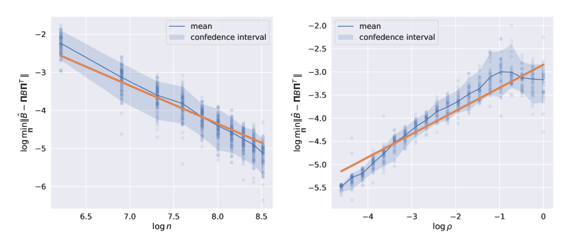
Figure 4: Convergence rate of SPOC++. See the description of setup in Section 4.2. On the left subfigure, we draw a red line with slope equals $-1$ to illustrate that the predicted rate of convergence is at most as observed. On the right subfigure, we draw a red line with slope equals $-1/2$ to illustrate the same. In both cases, we choose the intercept to minimize the mean squared distance to the observed errors.

We plot the error curves in logarithmic coordinates to estimate the convergence rate. The results are presented in Figure 4, left. It is easy to see that the observed error rate is a bit faster than the predicted one. The slope of the mean error is $-1.21\pm 0.03$. However, it does not contradict the theory since the provided lower bound holds for some matrix $\mathbf{B}$ that may not occur in the experiment.

We fix $n=5000$ for the second experiment and generate some matrix $\mathbf{P}$ as before. Then, we generate 40 symmetric matrices $\mathbf{E}^{(1)},\ldots,\mathbf{E}^{(40)}\in[0,1]^{n\times n}$. Entries of each matrix $\mathbf{E}^{(p)}$ are uniformly distributed random variables with the support $[0,1]$. Given the sparsity parameter $\rho$ and a matrix $\mathbf{E}^{(p)}$, we generate a matrix $\mathbf{A}$ as follows:

$$\mathbf{A}_{ij}={\operatorname{I}\left\{\mathbf{E}^{(p)}_{ij}<\rho\cdot\mathbf{P}_{ij}\right\}}.$$

We apply our algorithm to $\mathbf{A}$ and compute the error of ${\widehat{\mathbf{B}}}$.

We study our algorithm for 20 different values of $\rho$. The results are presented on Figure 4, right. Visually, the observed rate of convergence is a bit faster than the predicted. We calculate the slope of the mean error which turns out to be $0.56\pm 0.03$.

4.3 Comparison with other algorithms

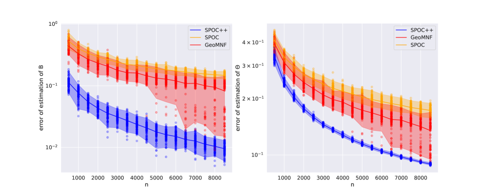
Figure 5: Error of reconstruction of $\mathbf{B}$ and $\boldsymbol{\mathrm{\Theta}}$ for different algorithms. See setup in Section 4.3.

We compare the performance of our algorithm with Algorithm 2 and GeoMNF (Mao et al., 2017), as other distribution-free algorithms are similar to Algorithm 2. We set the number of communities to $3$. As in Section 4.2, we generate a well-conditioned matrix $\bar{\mathbf{B}}$, then, for each $n\in\{500,1000,\ldots,8500\}$, we choose $\rho=1$ and generate a matrix $\mathbf{P}$. As previously, for each community, the number of pure nodes was equal to $0.09\cdot n$, and membership vectors of non-pure nodes were sampled from the $Dirichlet(1,1,1)$ distribution. Given a matrix of connection probabilities $\mathbf{P}$, we generate 40 different matrices $\mathbf{A}$, and for each of them, we compute the error of reconstruction of $\mathbf{B}$ and $\boldsymbol{\mathrm{\Theta}}$, defined as follows:

$$\mathcal{L}_{\mathbf{B}}(\mathbf{B},{\widehat{\mathbf{B}}})=\min_{\mathbf{\Pi}\in\mathbb{S}_{K}}\|{\widehat{\mathbf{B}}}-\mathbf{\Pi}^{\mathrm{T}}\mathbf{B}\mathbf{\Pi}\|_{\mathrm{F}},\quad\mathcal{L}_{\boldsymbol{\mathrm{\Theta}}}(\boldsymbol{\mathrm{\Theta}},{\widehat{\boldsymbol{\mathrm{\Theta}}}})=\min_{\mathbf{\Pi}\in\mathbb{S}_{K}}\frac{\|{\widehat{\boldsymbol{\mathrm{\Theta}}}}-\boldsymbol{\mathrm{\Theta}}\mathbf{\Pi}\|_{\mathrm{F}}}{\|\boldsymbol{\mathrm{\Theta}}\|_{\mathrm{F}}}.$$

The results are presented in Figure 5. As one can see, our algorithm significantly outperforms Algorithm 2 and GeoMNF.

5 Discussion

The most important assumption we made is Condition 4 since it allows us to reduce the error rate significantly. The lower bound was also obtained under this condition. We conjecture that if Condition 4 does not hold, then the lower bound from Theorem 3 is no longer optimal. We think it can be obtained by constructing families $\mathcal{B}$ of community matrices and $\mathcal{T}$ of membership matrices such that $|\mathcal{P}_{k}|=1$, $k\in[K]$, for each $\boldsymbol{\mathrm{\Theta}}\in\mathcal{T}$. However, this analysis is out of the scope of our paper.

Let us note that Condition 4 covers the important intermediate case between Stochastic Block Model and Mixed-Membership Stochastic Block Model with almost no pure nodes. Thus, it seems pretty natural and can be satisfied in practice.

Appendix A Proof of Proposition 1

Let us estimate eigenvalues of matrix $\mathbf{\Sigma}(i,j)$. After some straightforward calculations, we have

$$\mathbf{\Sigma}(i,j) =\mathbf{L}^{-1}\mathbf{U}^{\mathrm{T}}\mathbb{E}\left(\mathbf{W}_{i}-\mathbf{W}_{j}\right)^{\mathrm{T}}\left(\mathbf{W}_{i}-\mathbf{W}_{j}\right)\mathbf{U}\mathbf{L}^{-1}$$

$$=\mathbf{L}^{-1}\mathbf{U}^{\mathrm{T}}\left(\operatorname{diag}(\mathbb{E}\mathbf{W}_{i}^{2}+\mathbb{E}\mathbf{W}_{j}^{2})-\mathbb{E}\mathbf{W}_{ij}^{2}(\mathbf{e}_{i}\mathbf{e}_{j}^{\mathrm{T}}+\mathbf{e}_{j}\mathbf{e}_{i}^{\mathrm{T}})\right)\mathbf{U}\mathbf{L}^{-1}.$$ (17)

The maximum eigenvalue can be estimated using a norm of the matrix:

$$\lambda_{\max}\bigl{(}\mathbf{\Sigma}(i,j)\bigr{)}=\|\mathbf{\Sigma}(i,j)\|\leqslant\|\mathbf{L}^{-1}\|^{2}\|\mathbf{U}\|^{2}\left(\|\operatorname{diag}(\mathbb{E}\mathbf{W}_{i}^{2}+\mathbb{E}\mathbf{W}_{j}^{2})\|+2\mathbb{E}\mathbf{W}_{ij}^{2}\right),$$

$$\lambda_{\max}\bigl{(}\mathbf{\Sigma}(i,j)\bigr{)}\leqslant\frac{4\rho}{\lambda_{K}^{2}(\mathbf{P})},$$

since $\mathbb{E}\mathbf{W}_{ij}^{2}=\mathbf{P}_{ij}-\mathbf{P}_{ij}^{2}$. Due to Lemma 25, we have $\lambda_{K}^{2}(\mathbf{P})=\Omega(n\rho)$, so the upper bound holds. To find the lower bound of the minimal eigenvalue of $\mathbf{\Sigma}(i,j)$, we need Condition 4. Let us rewrite (A) in the following way:

$$\mathbf{\Sigma}(i,j)=\mathbf{L}^{-1}\bigl{(}\mathbf{S}_{1}(i,j)+\mathbf{S}_{2}(i,j)-\mathbf{S}_{3}(i,j)\bigr{)}\mathbf{L}^{-1},$$

where

$$\mathbf{S}_{1}(i,j) =\sum_{m\in\mathcal{P}}\left(\mathbb{E}\mathbf{W}_{im}^{2}+\mathbb{E}\mathbf{W}_{jm}^{2}\right)\mathbf{U}_{m}^{\mathrm{T}}\mathbf{U}_{m},$$

$$\mathbf{S}_{2}(i,j) =\sum_{m\not\in\mathcal{P}}\left(\mathbb{E}\mathbf{W}_{im}^{2}+\mathbb{E}\mathbf{W}_{jm}^{2}\right)\mathbf{U}_{m}^{\mathrm{T}}\mathbf{U}_{m},$$

$$\mathbf{S}_{3}(i,j) =\mathbb{E}\mathbf{W}_{ij}^{2}\left(\mathbf{U}_{i}^{\mathrm{T}}\mathbf{U}_{j}+\mathbf{U}_{j}^{\mathrm{T}}\mathbf{U}_{i}\right).$$

Now we analyze $\mathbf{S}_{1}(i,j)$. Since $\mathbf{U}=\boldsymbol{\mathrm{\Theta}}\mathbf{F}$, we obtain

$$\mathbf{S}_{1}(i,j) =\sum_{k=1}^{K}n_{k}\left(\boldsymbol{\mathrm{\Theta}}_{i}\mathbf{B}_{k}^{\mathrm{T}}-(\boldsymbol{\mathrm{\Theta}}_{i}\mathbf{B}_{k}^{\mathrm{T}})^{2}+\left(\boldsymbol{\mathrm{\Theta}}_{j}\mathbf{B}_{k}^{\mathrm{T}}-(\boldsymbol{\mathrm{\Theta}}_{j}\mathbf{B}_{k}^{\mathrm{T}})^{2}\right)\right)\mathbf{F}_{k}^{\mathrm{T}}\mathbf{F}_{k}$$

$$\geqslant 2\sum_{k=1}^{K}n_{k}\min\left\{\min_{k^{\prime}}\mathbf{B}_{k^{\prime}k}-(\min_{k^{\prime}}\mathbf{B}_{k^{\prime}k})^{2},\max_{k^{\prime}}\mathbf{B}_{k^{\prime}k}-(\max_{k^{\prime}}\mathbf{B}_{k^{\prime}k})^{2}\right\}\mathbf{F}_{k}^{\mathrm{T}}\mathbf{F}_{k}$$

$$=n\rho\sum_{k=1}^{K}\alpha_{k}\mathbf{F}_{k}^{\mathrm{T}}\mathbf{F}_{k},$$

where $\alpha_{k}$, $k\in[K]$ are bounded away from 0 since entries of $\mathbf{B}$ are bounded away from 0 and 1 by the assumptions of the proposition. Lemma 24 implies that there are such constants $C_{1},C_{2}$ that

$$\rho C_{1}\leqslant\lambda_{\min}\bigl{(}\mathbf{S}_{1}(i,j)\bigr{)}\leqslant\lambda_{\max}\bigl{(}\mathbf{S}_{1}(i,j)\bigr{)}\leqslant\rho C_{2}.$$

Since $\mathbf{S}_{2}(i,j)$ is non-negative defined, we state that $\lambda_{\min}\bigl{(}\mathbf{S}_{2}(i,j)\bigr{)}\geqslant 0$.

In order to estimate eigenvalues of $\mathbf{S}_{3}(i,j)$, we use Lemma 26:

$$\lambda_{\max}\bigl{(}\mathbf{S}_{3}(i,j)\bigr{)}\leqslant\rho\left(\|\mathbf{U}_{i}^{\mathrm{T}}\mathbf{U}_{j}\|+\|\mathbf{U}_{j}^{\mathrm{T}}\mathbf{U}_{i}\|\right)\leqslant\frac{2\rho KC_{\mathbf{U}}^{2}}{n}.$$

Applying multiplicative Weyl’s inequality, we get

$$\lambda_{\min}\bigl{(}\mathbf{\Sigma}(i,j)\bigr{)}\geqslant\frac{1}{\lambda^{2}_{K}(\mathbf{P})}\bigl{[}\lambda_{\min}\bigl{(}\mathbf{S}_{1}(i,j)\bigr{)}-\lambda_{\max}\bigl{(}\mathbf{S}_{3}(i,j)\bigr{)}\bigr{]}\geqslant\frac{1}{n^{2}\rho}\left(c_{1}-\frac{c_{2}}{n}\right)$$ (18)

for some positive constants $c_{1}$, $c_{2}$. Thus, the proposition follows.

Appendix B Proofs for Theorem 2

Here and further following Fan et al. (2022) we use the notation $O_{\prec}(\cdot)$:

Definition 4.

Suppose $\xi$ and $\eta$ to be random variables that may depend on $n$. We say that $\xi=O_{\prec}(\eta)$ if and only if for any positive $\varepsilon$ and $\delta$ there exists $n_{0}$ such that for any $n>n_{0}$

$$\mathbb{P}\left(|\xi|>n^{\varepsilon}|\eta|\right)\leqslant n^{-\delta}.$$ (19)

It is easy to check the following properties of $O_{\prec}(\cdot)$. If $\xi_{1}=O_{\prec}(\eta_{1})$ and $\xi_{2}=O_{\prec}(\eta_{2})$ then $\xi_{1}+\xi_{2}=O_{\prec}(|\eta_{1}|+|\eta_{2}|)$, $\xi_{1}+\xi_{2}=O_{\prec}\left(\max\{|\eta_{1}|,|\eta_{2}|\}\right)$ and $\xi_{1}\xi_{2}=O_{\prec}(\eta_{1}\eta_{2})$.

Additionally, we introduce a bit different type of convergence.

Definition 5.

Suppose $\xi$ and $\eta$ to be random variables that may depend on $n$. Say $\xi=O_{\ell}(\eta)$ if for any $\varepsilon>0$ there exist $n_{0}$ and $\delta>0$ such that

$$\mathbb{P}\left(\xi\geqslant\delta\eta\right)\leqslant n^{-\varepsilon}$$

holds for all $n\geqslant n_{0}$.

It preserves the properties of $O_{\prec}(\cdot)$ described previously. Moreover, $O_{\prec}(\eta)=O_{\ell}(n^{\alpha}\cdot\eta)$ for any $\alpha>0$.

Further, we have a lot of random variables $\xi_{i}$ depending on index $i\in[n]$. Mostly, they have the form $\mathbf{e}_{i}^{\mathrm{T}}\mathbf{X}$ for some random matrix $\mathbf{X}$. Formally, if $\xi_{i}=O_{\prec}(\eta_{n})$, we are not allowed to state $\max_{i}\xi_{i}=O_{\prec}(\eta_{n})$ since $n_{0}$ for different $i$ may be distinct and not be bounded. Nevertheless, the source of $O_{\prec}(\cdot)$ is random variables of the form $\mathbf{x}^{\mathrm{T}}(\mathbf{W}^{\ell}-\mathbb{E}\mathbf{W}^{\ell})\mathbf{y}$, that can be uniformly bounded using all moments provided by Lemma 32. Thus, $\xi_{i}=O_{\prec}(\eta_{n})$ for any $i\in S\subset[n]$ implies $\max_{i\in S}\|\xi_{i}\|_{2}=O_{\prec}(\eta_{n})$.

The order $O_{\ell}(\eta_{n})$ appears when we combine $O_{\prec}(\eta_{n}/n^{\alpha})$ for some $\alpha>0$ and random variable $X$ bounded by $\eta_{n}$ via Freedman or Bernstein inequalities that provide exactly the same $n_{0}$ for different $i$. Consequently, taking maximum over any subset of $[n]$ is also allowed.

B.1 Asymptotics of eigenvectors

The following lemma allows us to establish the behavior of eigenvectors.

Lemma 6.

Under Conditions 1-4 it holds that

$$\widehat{\mathbf{U}}_{ik} =\mathbf{U}_{ik}+\frac{\mathbf{e}_{i}^{\mathrm{T}}\mathbf{W}\mathbf{u}_{k}}{t_{k}}+\frac{\mathbf{e}_{i}^{\mathrm{T}}\mathbf{W}^{2}\mathbf{u}_{k}}{t_{k}^{2}}-\frac{3}{2}\cdot\mathbf{U}_{ik}\frac{\mathbf{u}_{k}^{\mathrm{T}}\mathbb{E}\mathbf{W}^{2}\mathbf{u}_{k}}{t_{k}^{2}}$$

$$\quad\,+\frac{1}{t_{k}^{2}}\sum_{k^{\prime}\in[K]\setminus\{k\}}\frac{\lambda_{k^{\prime}}\mathbf{U}_{ik^{\prime}}}{\lambda_{k^{\prime}}-t_{k}}\cdot\mathbf{u}_{k^{\prime}}^{\mathrm{T}}\mathbb{E}\mathbf{W}^{2}\mathbf{u}_{k}+O_{\ell}\left(\sqrt{\frac{\log n}{n^{3}\rho}}\right).$$

Proof  For further derivations, we need to introduce some notations. All necessary variables are defined in Table 2. Then, we define $t_{k}$ as a solution of

$$1+\lambda_{k}(\mathbf{P})\left\{\mathcal{R}(\mathbf{u}_{k},\mathbf{u}_{k},z)-\mathcal{R}(\mathbf{u}_{k},\mathbf{U}_{-k},z)[\mathbf{L}^{-1}_{-k}+\mathcal{R}(\mathbf{U}_{-k},\mathbf{U}_{-k},z)]^{-1}\mathcal{R}(\mathbf{U}_{-k},\mathbf{u}_{k},z)\right\}=0$$ (20)

on the closed interval $[a_{k},b_{k}]$, where

$$a_{k}=\begin{cases}\lambda_{k}(\mathbf{P})/(1+2^{-1}c_{0}),&\lambda_{k}(\mathbf{P})>0,\\ (1+2^{-1}c_{0})\lambda_{k}(\mathbf{P}),&\lambda_{k}(\mathbf{P})<0,\end{cases}\text{ and }b_{k}=\begin{cases}(1+2^{-1}c_{0})\lambda_{k}(\mathbf{P}),&\lambda_{k}(\mathbf{P})>0,\\ \lambda_{k}(\mathbf{P})/(1+2^{-1}c_{0}),&\lambda_{k}(\mathbf{P})<0,\end{cases}$$

and $c_{0}$ is defined in Condition 3.

Throughout this proof, a lot of auxiliary variables appear. For them, we exploit asymptotics established in Lemma 19. Lemma 21 guarantees that $\mathbf{x}^{\mathrm{T}}\mathbf{W}\mathbf{y}=O_{\ell}(\sqrt{\rho\log n})$ whenever unit $\mathbf{x}$ or $\mathbf{y}$ is $\mathbf{u}_{k}$ because of Condition 2 ($\rho\gg n^{-1/3}$) and Lemma 26 ($\|\mathbf{u}_{k}\|_{\infty}=O(n^{-1/2}$)). Thus, any term of the form $\mathbf{v}^{\mathrm{T}}\mathbf{W}\mathbf{u}_{k}$ becomes

$$\mathbf{v}^{\mathrm{T}}\mathbf{W}\mathbf{u}_{k}=O_{\ell}(\sqrt{\rho\log n})\cdot\|\mathbf{v}\|_{2}.$$

First, from Lemma 20,

$$\mathbf{u}_{k}^{\mathrm{T}}{\widehat{\mathbf{u}}}_{k}{\widehat{\mathbf{u}}}_{k}^{\mathrm{T}}\mathbf{u}_{k} =A_{\mathbf{u}_{k},k,t_{k}}A_{\mathbf{u}_{k},k,t_{k}}\widetilde{\mathcal{P}}_{k,t_{k}}+\operatorname{tr}\left[\mathbf{W}\mathbf{J}_{\mathbf{u}_{k},\mathbf{u}_{k},k,t_{k}}-(\mathbf{W}^{2}-\mathbb{E}\mathbf{W}^{2})\mathbf{L}_{\mathbf{u}_{k},\mathbf{u}_{k},k,t_{k}}\right]$$

$$+\operatorname{tr}(\mathbf{W}\mathbf{u}_{k}\mathbf{u}_{k}^{\mathrm{T}})\operatorname{tr}(\mathbf{W}\mathbf{Q}_{\mathbf{u}_{k},\mathbf{u}_{k},k,t_{k}})+O_{\prec}\left(\frac{1}{n^{2}\rho^{2}}\right).$$

Notice, that $\mathbf{J}_{\mathbf{u}_{k},\mathbf{u}_{k},k,t_{k}}=\mathbf{u}_{k}\mathbf{v}^{\mathrm{T}}_{\mathbf{J}}$ for

$$\mathbf{v}_{\mathbf{J}}^{\mathrm{T}} =-2A_{\mathbf{u}_{k},k,t_{k}}\widetilde{\mathcal{P}}_{k,t_{k}}t_{k}^{-1}\left(\mathbf{b}_{\mathbf{u}_{k},k,t_{k}}^{\mathrm{T}}+A_{\mathbf{u}_{k},k,t_{k}}\widetilde{\mathcal{P}}_{k,t_{k}}\mathbf{u}_{k}^{\mathrm{T}}\right)$$

$$=-2\left[-1-\frac{\mathbf{u}_{k}^{\mathrm{T}}\mathbb{E}\mathbf{W}^{2}\mathbf{u}_{k}}{t_{k}^{2}}+O(t_{k}^{-3/2})\right]\times\left[1-\frac{3}{t_{k}^{2}}\mathbf{u}_{k}^{\mathrm{T}}\mathbb{E}\mathbf{W}^{2}\mathbf{u}_{k}+O(t_{k}^{-3/2})\right]t_{k}^{-1}\times$$

$$\quad\,\times\left[\mathbf{u}_{k}+O(t_{k}^{-1})+\left(-1-\frac{\mathbf{u}_{k}^{\mathrm{T}}\mathbb{E}\mathbf{W}^{2}\mathbf{u}_{k}}{t_{k}^{2}}+O(t_{k}^{-3/2})\right)\left(1-\frac{3}{t_{k}^{2}}\mathbf{u}_{k}^{\mathrm{T}}\mathbb{E}\mathbf{W}^{2}\mathbf{u}_{k}+O(t_{k}^{-3/2})\right)\mathbf{u}_{k}\right]^{\mathrm{T}}$$

$$=O(t_{k}^{-2}),$$

where we use Lemma 33 for estimation of $\mathbf{u}_{k}^{\mathrm{T}}\mathbb{E}\mathbf{W}^{2}\mathbf{u}_{k}$ and Lemma 19 for asymptotic behaviour of the auxiliary variables. Consequently,

$$\operatorname{tr}(\mathbf{W}\mathbf{J}_{\mathbf{u}_{k},\mathbf{u}_{k},k,t_{k}})=O_{\ell}\left(\frac{\sqrt{\rho\log n}}{n^{2}\rho^{2}}\right)$$

because $t_{k}=\Theta\bigl{(}\lambda_{k}(\mathbf{P})\bigr{)}$ due to Lemma 27 and $\lambda_{k}(\mathbf{P})=\Theta(n\rho)$ due to Lemma 25.

Next, consider $\mathbf{L}_{\mathbf{u}_{k},\mathbf{u}_{k},k,t_{k}}$ which is also can represented as $\mathbf{u}_{k}\mathbf{v}_{\mathbf{L}}^{\mathrm{T}}$, where

$$\mathbf{v}_{\mathbf{L}}=\widetilde{\mathcal{P}}_{k,t_{k}}t_{k}^{-2}\big{(}(3A^{2}_{\mathbf{u}_{k},k,t_{k}}+2A_{\mathbf{u}_{k},k,t_{k}})\mathbf{u}_{k}+2A_{\mathbf{u}_{k},k,t_{k}}\mathbf{U}_{-k}[\mathbf{L}^{-1}_{-k}+\mathcal{R}(\mathbf{U}_{-k},\mathbf{U}_{-k},t_{k})]^{-1}\mathcal{R}(\mathbf{u}_{k},\mathbf{U}_{-k},t_{k})^{\mathrm{T}}\big{)}.$$

According to Lemma 19, we have

$$\quad\left\|2A_{\mathbf{u}_{k},k,t_{k}}\mathbf{U}_{-k}[\mathbf{L}^{-1}_{-k}+\mathcal{R}(\mathbf{U}_{-k},\mathbf{U}_{-k},t_{k})]^{-1}\mathcal{R}(\mathbf{u}_{k},\mathbf{U}_{-k},t_{k})^{\mathrm{T}}\right\|$$

$$=O(1)\cdot\bigl{\|}[\mathbf{L}^{-1}_{-k}+\mathcal{R}(\mathbf{U}_{-k},\mathbf{U}_{-k},t_{k})]^{-1}\bigr{\|}\times t_{k}^{-3}\bigl{\|}\mathbf{u}_{k}^{\mathrm{T}}\mathbb{E}\mathbf{W}^{2}\mathbf{U}_{-k}\bigr{\|}=O(t_{k}^{-1}),$$

and, consequently,

$$\mathbf{v}_{\mathbf{L}}=\widetilde{\mathcal{P}}_{k,t_{k}}t_{k}^{-2}(3A_{\mathbf{u}_{k},k,t_{k}}^{2}+2A_{\mathbf{u}_{k},k,t_{k}})\mathbf{u}_{k}+O\bigl{(}t_{k}^{-3}\bigr{)}.$$

While $3A_{\mathbf{u}_{k},k,t_{k}}^{2}+2A_{\mathbf{u}_{k},k,t_{k}}=3+\frac{6\mathbf{u}_{k}^{\mathrm{T}}\mathbb{E}\mathbf{W}^{2}\mathbf{u}_{k}}{t_{k}^{2}}+O(t_{k}^{-3/2})-2-\frac{2\mathbf{u}_{k}^{\mathrm{T}}\mathbb{E}\mathbf{W}\mathbf{u}_{k}}{t_{k}^{2}}+O(t_{k}^{-3/2})=1+4\cdot\frac{\mathbf{u}_{k}^{\mathrm{T}}\mathbb{E}\mathbf{W}^{2}\mathbf{u}_{k}}{t_{k}^{2}}+O(t_{k}^{-3/2})$, and, hence,

$$\mathbf{v}_{\mathbf{L}}=\left(1+\frac{\mathbf{u}_{k}^{\mathrm{T}}\mathbb{E}\mathbf{W}^{2}\mathbf{u}_{k}}{t_{k}^{2}}\right)\cdot t_{k}^{-2}\mathbf{u}_{k}+O(t_{k}^{-7/2})=t_{k}^{-2}\mathbf{u}_{k}+O(t_{k}^{-3}).$$

That implies

$$\operatorname{tr}\bigl{[}(\mathbf{W}^{2}-\mathbb{E}\mathbf{W}^{2})\mathbf{L}_{\mathbf{u}_{k},\mathbf{u}_{k},k,t_{k}}\bigr{]} =\frac{\mathbf{u}_{k}^{\mathrm{T}}(\mathbf{W}^{2}-\mathbb{E}\mathbf{W}^{2})\mathbf{u}_{k}}{t_{k}^{2}}+O(t_{k}^{-3})\cdot O_{\prec}(t_{k}^{1/2})$$

$$=\frac{\mathbf{u}_{k}^{\mathrm{T}}(\mathbf{W}^{2}-\mathbb{E}\mathbf{W}^{2})\mathbf{u}_{k}}{t_{k}^{2}}+O_{\prec}(t_{k}^{-5/2}),$$

where Lemma 32 was used.

Next, representing $\mathbf{Q}_{\mathbf{u}_{k},\mathbf{u}_{k},k,t_{k}}$ as $\mathbf{u}_{k}\mathbf{v}_{\mathbf{Q}}$ with

$$\mathbf{v}_{\mathbf{Q}}=\mathbf{v}_{\mathbf{L}}-\widetilde{\mathcal{P}}_{k,t_{k}}t_{k}^{-2}A_{\mathbf{u}_{k},k,t_{k}}^{2}\mathbf{u}_{k}+4\widetilde{\mathcal{P}}^{2}t_{k}^{-2}A_{\mathbf{u}_{k},k,t_{k}}\mathbf{b}_{\mathbf{u}_{k},k,t_{k}}=O(t_{k}^{-2}),$$

we obtain

$$\operatorname{tr}(\mathbf{W}\mathbf{u}_{k}\mathbf{u}_{k}^{\mathrm{T}})\operatorname{tr}(\mathbf{W}\mathbf{Q}_{\mathbf{u}_{k},\mathbf{u}_{k},k,t_{k}})=O_{\ell}(\sqrt{\rho\log n})\cdot O_{\ell}(\sqrt{\rho\log n})\cdot O(t_{k}^{-2})=O_{\ell}(\rho\cdot t_{k}^{-2}\log n).$$

Finally, obtained via Lemma 19, the decomposition

$$\widetilde{\mathcal{P}}_{k,t_{k}}A_{\mathbf{u}_{k},k,t_{k}}^{2}=1-\frac{\mathbf{u}_{k}^{\mathrm{T}}\mathbb{E}\mathbf{W}^{2}\mathbf{u}_{k}}{t_{k}^{2}}+O\bigl{(}t_{k}^{-3/2}\bigr{)}.$$

provides us with expansion

$$\mathbf{u}_{k}^{\mathrm{T}}{\widehat{\mathbf{u}}}_{k}{\widehat{\mathbf{u}}}_{k}^{\mathrm{T}}\mathbf{u}_{k}=1-\frac{\mathbf{u}_{k}^{\mathrm{T}}\mathbf{W}^{2}\mathbf{u}_{k}}{t_{k}^{2}}+O_{\ell}\bigl{(}t_{k}^{-3/2}\bigr{)},$$

$$\langle\mathbf{u}_{k},{\widehat{\mathbf{u}}}_{k}\rangle=1-\frac{\mathbf{u}_{k}^{\mathrm{T}}\mathbf{W}^{2}\mathbf{u}_{k}}{2t_{k}^{2}}+O_{\ell}\bigl{(}t_{k}^{-3/2}\bigr{)}.$$ (21)

Now, we should estimate

$$\mathbf{e}_{i}^{\mathrm{T}}{\widehat{\mathbf{u}}}_{k}{\widehat{\mathbf{u}}}_{k}^{\mathrm{T}}\mathbf{u}_{k}= A_{\mathbf{e}_{i},k,t_{k}}A_{\mathbf{u}_{k},k,t_{k}}\widetilde{\mathcal{P}}_{k,t_{k}}+\operatorname{tr}\left[\mathbf{W}\mathbf{J}_{\mathbf{e}_{i},\mathbf{u}_{k},k,t_{k}}-(\mathbf{W}^{2}-\mathbb{E}\mathbf{W}^{2})\mathbf{L}_{\mathbf{e}_{i},\mathbf{u}_{k},k,t_{k}}\right]$$

$$+\operatorname{tr}(\mathbf{W}\mathbf{u}_{k}\mathbf{u}_{k}^{\mathrm{T}})\operatorname{tr}(\mathbf{W}\mathbf{Q}_{\mathbf{e}_{i},\mathbf{u}_{k},k,t_{k}})+O_{\prec}\left(\frac{1}{n^{2}\rho^{2}}\right),$$

obtained from Lemma 20. For a reminder

$$\mathbf{J}_{\mathbf{e}_{i},\mathbf{u}_{k},k,t_{k}} =-\widetilde{\mathcal{P}}_{k,t_{k}}t_{k}^{-1}\mathbf{u}_{k}\left(A_{\mathbf{e}_{i},k,t_{k}}\mathbf{b}_{\mathbf{u}_{k},k,t_{k}}^{\mathrm{T}}+A_{\mathbf{u}_{k},k,t_{k}}\mathbf{b}_{\mathbf{e}_{i},k,t_{k}}^{\mathrm{T}}+2A_{\mathbf{u}_{k},k,t_{k}}A_{\mathbf{e}_{i},k,t_{k}}\widetilde{\mathcal{P}}_{k,t_{k}}\mathbf{u}_{k}^{\mathrm{T}}\right),$$

$$\mathbf{L}_{\mathbf{e}_{i},\mathbf{u}_{k},k,t_{k}} =\widetilde{\mathcal{P}}_{k,t_{k}}t_{k}^{-2}\mathbf{u}_{k}\bigg{\{}\bigl{[}A_{\mathbf{u}_{k},k,t_{k}}\mathcal{R}(\mathbf{e}_{i},\mathbf{U}_{-k},t_{k})+A_{\mathbf{e}_{i},k,t_{k}}\mathcal{R}(\mathbf{u}_{k},\mathbf{U}_{-k},t_{k})\bigr{]}$$

$$\quad\,\times\left[\mathbf{L}_{-k}^{-1}+\mathcal{R}(\mathbf{U}_{-k},\mathbf{U}_{-k},t_{k})\right]^{-1}\mathbf{U}_{-k}+A_{\mathbf{e}_{i},k,t_{k}}\mathbf{u}_{k}^{\mathrm{T}}+A_{\mathbf{u}_{k},k,t_{k}}\mathbf{e}_{i}^{\mathrm{T}}+3A_{\mathbf{e}_{i},k,t_{k}}A_{\mathbf{u}_{k},k,t_{k}}\mathbf{u}_{k}^{\mathrm{T}}\bigg{\}},$$

$$\mathbf{Q}_{\mathbf{e}_{i},\mathbf{u}_{k},k,t_{k}} =\mathbf{L}_{\mathbf{e}_{i},\mathbf{u}_{k},k,t_{k}}-\widetilde{\mathcal{P}}_{k,t_{k}}t_{k}^{-2}A_{\mathbf{e}_{i},k,t_{k}}A_{\mathbf{u}_{k},k,t_{k}}\mathbf{u}_{k}\mathbf{u}_{k}^{\mathrm{T}}+2\widetilde{\mathcal{P}}_{k,t_{k}}^{2}t_{k}^{-2}\mathbf{u}_{k}\left(A_{\mathbf{e}_{i},k,t_{k}}\mathbf{b}_{\mathbf{e}_{i},k,t_{k}}^{\mathrm{T}}+A_{\mathbf{u}_{k},k,t_{k}}\mathbf{b}_{\mathbf{u}_{k},k,t_{k}}^{\mathrm{T}}\right).$$

Applying asymptotic expansions from Lemma 19, we obtain

$$A_{\mathbf{u}_{k},k,t_{k}}\mathbf{b}_{\mathbf{e}_{i},k,t_{k}}^{\mathrm{T}} =\left(-1-\frac{\mathbf{u}_{k}^{\mathrm{T}}\mathbb{E}\mathbf{W}^{2}\mathbf{u}_{k}}{t_{k}^{2}}+O(t_{k}^{-3/2})\right)\times\left(\mathbf{e}_{i}+O(n^{-1/2})\right)=-\mathbf{e}_{i}+O(n^{-1/2}),$$

$$A_{\mathbf{e}_{i},k,t_{k}}\mathbf{b}_{\mathbf{u}_{k},k,t_{k}}^{\mathrm{T}} =\left(-\mathbf{U}_{ik}+O(t_{k}^{-1}/\sqrt{n})\right)\times\left(\mathbf{u}_{k}+O(t_{k}^{-1})\right)=-\mathbf{U}_{ik}\mathbf{u}_{k}+O(t_{k}^{-1}/\sqrt{n})=O(n^{-1/2}),$$

$$2A_{\mathbf{u}_{k},k,t_{k}}A_{\mathbf{e}_{i},k,t_{k}}\widetilde{\mathcal{P}}_{k,t_{k}}\mathbf{u}_{k}^{\mathrm{T}} =O(n^{-1/2}).$$

Using the same notation as previously, we observe

$$\mathbf{v}_{\mathbf{J}} =t_{k}^{-1}\mathbf{e}_{i}+O(t_{k}^{-1}n^{-1/2}),$$

$$\operatorname{tr}(\mathbf{W}\mathbf{J}_{\mathbf{e}_{i},\mathbf{u}_{k},k,t_{k}}) =\frac{\mathbf{e}_{i}^{\mathrm{T}}\mathbf{W}\mathbf{u}_{k}}{t_{k}}+O_{\ell}\left(\sqrt{\frac{\log n}{n^{3}\rho}}\right).$$

To estimate $\operatorname{tr}\bigl{[}(\mathbf{W}^{2}-\mathbb{E}\mathbf{W}^{2})\mathbf{L}_{\mathbf{e}_{i},\mathbf{u}_{k},k,t_{k}}\bigr{]}$, we obtain

$$\bigl{[}A_{\mathbf{u}_{k},k,t_{k}}\mathcal{R}(\mathbf{e}_{i},\mathbf{U}_{-k},t_{k})+A_{\mathbf{e}_{i},k,t_{k}}\mathcal{R}(\mathbf{u}_{k},\mathbf{U}_{-k},t_{k})\bigr{]}\left[\mathbf{L}_{-k}^{-1}+\mathcal{R}(\mathbf{U}_{-k},\mathbf{U}_{-k},t_{k})\right]^{-1}\mathbf{U}_{-k}$$

$$=\left[(-1+O(t_{k}^{-1}))\left(-\frac{1}{t_{k}}\mathbf{e}_{i}^{\mathrm{T}}\mathbf{U}_{-k}+O(t_{k}^{-2}/\sqrt{n})\right)+(-\mathbf{U}_{ik}+O(t_{k}^{-1}/\sqrt{n}))(-t_{k}^{-3}\mathbf{u}_{k}^{\mathrm{T}}\mathbb{E}\mathbf{W}^{2}\mathbf{U}_{-k}+O(t_{k}^{-5/2})\right]$$

$$\quad\times\left(\operatorname{diag}\left(\frac{\lambda_{k^{\prime}}t_{k}}{t_{k}-\lambda_{k^{\prime}}}\right)_{k^{\prime}\in[K]\setminus\{k\}}+O(1)\right)\mathbf{U}_{-k}=\sum_{k^{\prime}\in[K]\setminus\{k\}}\frac{\lambda_{k^{\prime}}}{t_{k}-\lambda_{k^{\prime}}}\mathbf{U}_{ik^{\prime}}\mathbf{u}_{k^{\prime}}^{\mathrm{T}}+O(t_{k}^{-2}),$$

where we use Lemma 19 and $\mathbf{u}_{k}^{\mathrm{T}}\mathbb{E}\mathbf{W}^{2}\mathbf{u}_{k^{\prime}}=O(t_{k}),k^{\prime}\in[K]$, $\mathbf{e}_{i}^{\mathrm{T}}\mathbb{E}\mathbf{W}^{2}\mathbf{u}_{k}=O(t_{k}/\sqrt{n})$ from Lemma 33. Consequently, we have

$$\mathbf{v}_{\mathbf{L}} =-\frac{\mathbf{e}_{i}}{t_{k}^{2}}+t_{k}^{-2}\sum_{k^{\prime}\in[K]\setminus\{k\}}\frac{\lambda_{k^{\prime}}}{t_{k}-\lambda_{k^{\prime}}}\mathbf{U}_{ik^{\prime}}\mathbf{u}_{k^{\prime}}$$

$$\quad-t_{k}^{-2}(\mathbf{U}_{ik}+O(t_{k}^{-1}/\sqrt{n}))\mathbf{u}_{k}+3t_{k}^{-2}(\mathbf{U}_{ik}+O(t_{k}^{-1}/\sqrt{n}))\mathbf{u}_{k}+O(t_{k}^{-2}/\sqrt{n})$$

$$=-\frac{\mathbf{e}_{i}}{t_{k}^{2}}+t_{k}^{-2}\sum_{k^{\prime}\in[K]\setminus\{k\}}\frac{\lambda_{k^{\prime}}}{t_{k}-\lambda_{k^{\prime}}}\mathbf{U}_{ik^{\prime}}+\frac{\mathbf{u}_{k}^{\mathrm{T}}\mathbb{E}\mathbf{W}^{2}\mathbf{u}_{k^{\prime}}}{t_{k}^{2}}\mathbf{u}_{k^{\prime}}+2t_{k}^{-2}\mathbf{U}_{ik}\mathbf{u}_{k}+O(t_{k}^{-2}/\sqrt{n}).$$

Thus, we get

$$\operatorname{tr}\bigl{[}(\mathbf{W}^{2}-\mathbb{E}\mathbf{W}^{2})\mathbf{L}_{\mathbf{e}_{i},\mathbf{u}_{k},k,t_{k}}\bigr{]}=\mathbf{v}_{\mathbf{L}}^{\mathrm{T}}(\mathbf{W}^{2}-\mathbb{E}\mathbf{W}^{2})\mathbf{u}_{k}$$

$$\overset{\text{Lemma\leavevmode\nobreak\ \ref{lemma: power deviation}}}{=}-\mathbf{e}_{i}^{\mathrm{T}}(\mathbf{W}^{2}-\mathbb{E}\mathbf{W}^{2})\mathbf{u}_{k}+t_{k}^{-2}\sum_{k^{\prime}\in[K]\setminus\{k\}}\frac{\lambda_{k^{\prime}}}{t_{k}-\lambda_{k^{\prime}}}\mathbf{U}_{ik^{\prime}}\cdot\mathbf{u}_{k^{\prime}}(\mathbf{W}^{2}-\mathbb{E}\mathbf{W}^{2})\mathbf{u}_{k}$$

$$\quad+2t_{k}^{-2}\mathbf{U}_{ik}\cdot\mathbf{u}_{k}^{\mathrm{T}}(\mathbf{W}^{2}-\mathbb{E}\mathbf{W}^{2})\mathbf{u}_{k}+O(t_{k}^{-2}/\sqrt{n})\cdot O_{\prec}(t_{k}/\sqrt{n})$$

$$\overset{\text{Lemma\leavevmode\nobreak\ \ref{lemma: W squared bilinear form}}}{=}-\frac{1}{t_{k}^{2}}\mathbf{e}_{i}^{\mathrm{T}}(\mathbf{W}^{2}-\mathbb{E}\mathbf{W}^{2})\mathbf{u}_{k}+O(t_{k}^{-2}/\sqrt{n})\cdot O_{\ell}(\rho\sqrt{n}\log n)+O_{\prec}\left(t_{k}^{-1}/n\right)$$

$$=-\frac{1}{t_{k}^{2}}\mathbf{e}_{i}^{\mathrm{T}}(\mathbf{W}^{2}-\mathbb{E}\mathbf{W}^{2})\mathbf{u}_{k}+O_{\ell}\left(\frac{\log n}{n^{2}\rho}\right)+O_{\prec}\left(\frac{1}{n^{2}\rho}\right).$$

Finally, we obtain

$$\mathbf{v}_{\mathbf{Q}}=\mathbf{v}_{\mathbf{L}}+O(t_{k}^{-2}),$$

and

$$\operatorname{tr}(\mathbf{W}\mathbf{u}_{k}\mathbf{u}_{k}^{\mathrm{T}})\operatorname{tr}(\mathbf{W}\mathbf{Q}_{\mathbf{e}_{i},\mathbf{u}_{k},k,t_{k}})=O_{\ell}(\sqrt{\rho\log n})\cdot O_{\ell}(\sqrt{\rho\log n})O(t_{k}^{-2})=O_{\ell}\left(\frac{\log n}{n^{2}\rho}\right).$$

Approximating $\widetilde{\mathcal{P}}_{k,t_{k}}A_{\mathbf{e}_{i},k,t_{k}}A_{\mathbf{u}_{k},k,t_{k}}$ with

$$\widetilde{\mathcal{P}}_{k,t_{k}}A_{\mathbf{e}_{i},k,t_{k}}A_{\mathbf{u}_{k},k,t_{k}} =\left(1-\frac{3}{t_{k}^{2}}\mathbf{u}_{k}^{\mathrm{T}}\mathbb{E}\mathbf{W}^{2}\mathbf{u}_{k}+O(t_{k}^{-3/2})\right)\left(1+\frac{\mathbf{u}_{k}^{\mathrm{T}}\mathbb{E}\mathbf{W}^{2}\mathbf{u}_{k}}{t_{k}^{2}}+O(t_{k}^{-3/2})\right)\times$$

$$\quad\,\times\left(\mathbf{U}_{ik}+\frac{\mathbf{e}_{i}^{\mathrm{T}}\mathbb{E}\mathbf{W}^{2}\mathbf{u}_{k}}{t_{k}^{2}}+\sum_{k^{\prime}\in[K]\setminus\{k\}}\frac{\lambda_{k^{\prime}}\mathbf{U}_{ik^{\prime}}}{\lambda_{k^{\prime}}-t_{k}}\cdot\frac{\mathbf{u}_{k^{\prime}}^{\mathrm{T}}\mathbb{E}\mathbf{W}^{2}\mathbf{u}_{k}}{t_{k}^{2}}+O(t_{k}^{-5/2})\right)$$

$$=\mathbf{U}_{ik}-\frac{2}{t_{k}^{2}}\mathbf{U}_{ik}\mathbf{u}_{k}^{\mathrm{T}}\mathbb{E}\mathbf{W}^{2}\mathbf{u}_{k}+\frac{1}{t_{k}^{2}}\mathbf{e}_{i}^{\mathrm{T}}\mathbb{E}\mathbf{W}^{2}\mathbf{u}_{k}$$

$$\quad\,+\frac{1}{t_{k}^{2}}\sum_{k^{\prime}\in[K]\setminus\{k\}}\frac{\lambda_{k^{\prime}}\mathbf{U}_{ik^{\prime}}}{\lambda_{k^{\prime}}-t_{k}}\cdot\mathbf{u}_{k^{\prime}}^{\mathrm{T}}\mathbb{E}\mathbf{W}^{2}\mathbf{u}_{k}+O(t_{k}^{-3/2}n^{-1/2}),$$

we obtain

$$\langle\mathbf{e}_{i},{\widehat{\mathbf{u}}}_{k}\rangle\langle{\widehat{\mathbf{u}}}_{k},\mathbf{u}_{k}\rangle =\mathbf{U}_{ik}+\frac{\mathbf{e}_{i}^{\mathrm{T}}\mathbf{W}\mathbf{u}_{k}}{t_{k}}+\frac{\mathbf{e}_{i}^{\mathrm{T}}\mathbf{W}^{2}\mathbf{u}_{k}}{t_{k}^{2}}-\frac{2}{t_{k}^{2}}\mathbf{U}_{ik}\mathbf{u}_{k}^{\mathrm{T}}\mathbb{E}\mathbf{W}^{2}\mathbf{u}_{k}$$

$$\quad\,+\frac{1}{t_{k}^{2}}\sum_{k^{\prime}\in[K]\setminus\{k\}}\frac{\lambda_{k^{\prime}}\mathbf{U}_{ik^{\prime}}}{\lambda_{k^{\prime}}-t_{k}}\cdot\mathbf{u}_{k^{\prime}}^{\mathrm{T}}\mathbb{E}\mathbf{W}^{2}\mathbf{u}_{k}+O_{\ell}\left(\sqrt{\frac{\log n}{n^{3}\rho}}\right).$$ (22)

Here we use Condition 2 to ensure that the reminder $O_{\prec}\left(\frac{1}{n^{2}\rho^{2}}\right)$ provided by Lemma 20 is less than $O_{\ell}\left(\sqrt{\frac{\log n}{n^{3}\rho}}\right)$. Dividing (22) by (21) results in:

$$\widehat{\mathbf{U}}_{ik} =\mathbf{U}_{ik}+\frac{\mathbf{e}_{i}^{\mathrm{T}}\mathbf{W}\mathbf{u}_{k}}{t_{k}}+\frac{\mathbf{e}_{i}^{\mathrm{T}}\mathbf{W}^{2}\mathbf{u}_{k}}{t_{k}^{2}}-2\mathbf{U}_{ik}\frac{\mathbf{u}_{k}^{\mathrm{T}}\mathbb{E}\mathbf{W}^{2}\mathbf{u}_{k}}{t_{k}^{2}}+\frac{1}{2}\mathbf{U}_{ik}\frac{\mathbf{u}_{k}^{\mathrm{T}}\mathbf{W}^{2}\mathbf{u}_{k}}{t_{k}^{2}}$$

$$\quad\,+\frac{1}{t_{k}^{2}}\sum_{k^{\prime}\in[K]\setminus\{k\}}\frac{\lambda_{k^{\prime}}\mathbf{U}_{ik^{\prime}}}{\lambda_{k^{\prime}}-t_{k}}\cdot\mathbf{u}_{k^{\prime}}^{\mathrm{T}}\mathbb{E}\mathbf{W}^{2}\mathbf{u}_{k}+O_{\ell}\left(\frac{\sqrt{\log n}}{n\sqrt{n\rho}}\right)$$

due to Lemma 14. Additionally, this lemma guarantees that

$$\mathbf{U}_{ik}\frac{\mathbf{u}_{k}^{\mathrm{T}}\mathbf{W}^{2}\mathbf{u}_{k}}{t_{k}^{2}}-\mathbf{U}_{ik}\frac{\mathbf{u}_{k}^{\mathrm{T}}\mathbb{E}\mathbf{W}^{2}\mathbf{u}_{k}}{t_{k}^{2}}=\mathbf{U}_{ik}\cdot O_{\ell}\left(\frac{\rho\sqrt{n}\log n}{n^{2}\rho^{2}}\right)=O_{\ell}\left(\frac{\log n}{n^{2}\rho}\right).$$

This leads us to the statement of the lemma.  

B.2 Pure sets approximation

The aim of this section is to investigate the difference between ${\widehat{\mathcal{P}}}_{k}=\{j\mid{\widehat{T}}_{i_{k}j}^{a}<t_{n}\}$ and $\mathcal{P}_{k}$. For a reminder, we have defined

$$\bar{T}^{a}_{ij} =(\mathbf{U}_{i}-\mathbf{U}_{j})\left(\mathbf{\Sigma}(i,j)+a\mathbf{I}\right)^{-1}(\mathbf{U}_{i}-\mathbf{U}_{j})^{\mathrm{T}},$$

$$T^{a}_{ij} =(\widehat{\mathbf{U}}_{i}-\widehat{\mathbf{U}}_{j})\left(\mathbf{\Sigma}(i,j)+a\mathbf{I}\right)^{-1}(\widehat{\mathbf{U}}_{i}-\widehat{\mathbf{U}}_{j})^{\mathrm{T}},$$

$${\widehat{T}}^{a}_{ij} =(\widehat{\mathbf{U}}_{i}-\widehat{\mathbf{U}}_{j})\left({\widehat{\mathbf{\Sigma}}}(i,j)+a\mathbf{I}\right)^{-1}(\widehat{\mathbf{U}}_{i}-\widehat{\mathbf{U}}_{j})^{\mathrm{T}}.$$

We start with concentration of ${\widehat{T}}_{ij}^{a}$.

Lemma 7.

Consider two arbitrary indices $i,j\in[n]$. Then for each $\varepsilon$ there exist $n_{0}\in\mathbb{N}$ and $\delta_{1},\delta_{2}>0$ such that for any $n\geqslant n_{0}$

$$\mathbb{P}\left(\bigl{|}{\widehat{T}}_{ij}-\bar{T}^{a}_{ij}\bigr{|}\geqslant\sqrt{n\rho}\|\boldsymbol{\mathrm{\Theta}}_{i}-\boldsymbol{\mathrm{\Theta}}_{j}\|_{2}\cdot\delta_{1}\sqrt{\log n}+\delta_{2}\log n+n^{1-1/12}\rho\|\boldsymbol{\mathrm{\Theta}}_{i}-\boldsymbol{\mathrm{\Theta}}_{j}\|^{2}\right)\leqslant n^{-\varepsilon}.$$

Proof  Define

$$\mathbf{\Sigma}_{a}(i,j)=\mathbf{\Sigma}(i,j)+a\mathbf{I},\quad\quad{\widehat{\mathbf{\Sigma}}}_{a}(i,j)={\widehat{\mathbf{\Sigma}}}(i,j)+a\mathbf{I}.$$

We denote $\xi_{i}=\widehat{\mathbf{U}}_{i}-\mathbf{U}_{i}-\mathbf{W}_{i}\mathbf{U}\mathbf{L}^{-1}$ and observe:

$$T^{a}_{ij}=\bar{T}^{a}_{ij}+(\mathbf{W}_{i}-\mathbf{W}_{j})\mathbf{U}\mathbf{L}^{-1}\mathbf{\Sigma}_{a}^{-1}(i,j)(\mathbf{U}_{i}-\mathbf{U}_{j})^{\mathrm{T}}+(\mathbf{W}_{i}-\mathbf{W}_{j})\mathbf{U}\mathbf{L}^{-1}\mathbf{\Sigma}_{a}(i,j)^{-1}\left(\widehat{\mathbf{U}}_{i}-\widehat{\mathbf{U}}_{j}\right)^{\mathrm{T}}$$

$$+(\xi_{i}-\xi_{j})\mathbf{\Sigma}_{a}(i,j)^{-1}(\mathbf{U}_{i}-\mathbf{U}_{j})^{\mathrm{T}}+(\xi_{i}-\xi_{j})\mathbf{\Sigma}_{a}(i,j)^{-1}(\widehat{\mathbf{U}}_{i}-\widehat{\mathbf{U}}_{j})^{\mathrm{T}}$$

$$=\, \bar{T}^{a}_{ij}+2(\mathbf{W}_{i}-\mathbf{W}_{j})\mathbf{U}\mathbf{L}^{-1}\mathbf{\Sigma}_{a}^{-1}(i,j)(\mathbf{U}_{i}-\mathbf{U}_{j})^{\mathrm{T}}+(\mathbf{W}_{i}-\mathbf{W}_{j})\mathbf{U}\mathbf{L}^{-1}\mathbf{\Sigma}_{a}(i,j)^{-1}\mathbf{L}^{-1}\mathbf{U}^{\mathrm{T}}(\mathbf{W}_{i}-\mathbf{W}_{j})^{\mathrm{T}}$$

$$+2(\xi_{i}-\xi_{j})\mathbf{\Sigma}_{a}(i,j)^{-1}\left(\mathbf{U}_{i}-\mathbf{U}_{j}+(\mathbf{W}_{i}-\mathbf{W}_{j})\mathbf{U}\mathbf{L}^{-1}\right)^{\mathrm{T}}+(\xi_{i}-\xi_{j})\mathbf{\Sigma}_{a}(i,j)^{-1}(\xi_{i}-\xi_{j})^{\mathrm{T}}.$$ (23)

Due to Lemma 21 and Lemma 26, we have $\mathbf{e}_{i}^{\mathrm{T}}\mathbf{W}\mathbf{u}_{k}=O_{\ell}(\sqrt{\rho\log n})$ for any $i$. So, from Lemma 25 we get

$$\mathbf{W}_{i}\mathbf{U}\mathbf{L}^{-1}=O_{\ell}(\sqrt{\rho\log n})\cdot O\Biggl{(}\frac{1}{n\rho}\Biggr{)}=O_{\ell}\Biggl{(}\frac{\sqrt{\log n}}{n\sqrt{\rho}}\Biggr{)},$$

Thus, we have

$$\max_{i,j}\|(\mathbf{W}_{i}-\mathbf{W}_{j})\mathbf{U}\mathbf{L}^{-1}\|_{2}=O_{\ell}\left(\frac{\sqrt{\log n}}{n\sqrt{\rho}}\right).$$ (24)

Besides, according to Lemma 30, we have $\xi_{i}=O_{\prec}\left(\frac{1}{\sqrt{n}n\rho}\right)$ and so

$$\max_{i,j}\|\xi_{i}-\xi_{j}\|_{2}=O_{\prec}\left(\frac{1}{\rho\sqrt{n^{3}}}\right)$$ (25)

holds. From Lemma 24 there is the constant $C$ such that

$$\left\|\mathbf{U}_{i}-\mathbf{U}_{j}\right\|_{2}\leqslant\frac{C_{1}\|\boldsymbol{\mathrm{\Theta}}_{i}-\boldsymbol{\mathrm{\Theta}}_{j}\|_{2}}{\sqrt{n}}.$$ (26)

In addition, from Lemma 17 we get $\|\mathbf{\Sigma}_{a}(i,j)^{-1}\|_{2}\leqslant C_{2}n^{2}\rho$ for some constant $C_{2}$. Define $\Delta_{ij}=\|\boldsymbol{\mathrm{\Theta}}_{i}-\boldsymbol{\mathrm{\Theta}}_{j}\|_{2}$. Using bounds (24)-(26), we may bound all terms of (B.2) uniformly over $i$ and $j$ as follows:

$$(i)\quad \bigl{\|}2(\mathbf{W}_{i}-\mathbf{W}_{j})\mathbf{U}\mathbf{L}^{-1}\mathbf{\Sigma}_{a}^{-1}(i,j)(\mathbf{U}_{i}-\mathbf{U}_{j})^{\mathrm{T}}\bigr{\|}_{2}\leqslant 2\|(\mathbf{W}_{i}-\mathbf{W}_{j})\mathbf{U}\mathbf{L}^{-1}\|_{2}\cdot\|\mathbf{\Sigma}_{a}^{-1}(i,j)\|_{2}\cdot\|\mathbf{U}_{i}-\mathbf{U}_{j}\|_{2}$$

$$=\leavevmode\nobreak\ O_{\ell}\left(\frac{\sqrt{\log n}}{n\sqrt{\rho}}\right)\cdot O(n^{2}\rho)\cdot O\left(n^{-1/2}\right)\Delta_{ij}=O_{\ell}\left(\sqrt{n\rho\log n}\right)\Delta_{ij},$$

$$(ii)\quad \bigl{\|}(\mathbf{W}_{i}-\mathbf{W}_{j})\mathbf{U}\mathbf{L}^{-1}\mathbf{\Sigma}_{a}(i,j)^{-1}\mathbf{L}^{-1}\mathbf{U}^{\mathrm{T}}(\mathbf{W}_{i}-\mathbf{W}_{j})^{\mathrm{T}}\bigr{\|}_{2}\leqslant\|(\mathbf{W}_{i}-\mathbf{W}_{j})\mathbf{U}\mathbf{L}^{-1}\|_{2}^{2}\cdot\|\mathbf{\Sigma}_{a}(i,j)^{-1}\|_{2}$$

$$=\leavevmode\nobreak\ O_{\ell}\left(\frac{\log n}{n^{2}\rho}\right)O(n^{2}\rho)=O_{\ell}\left(\log n\right),$$

$$(iii)\quad \bigl{\|}2(\xi_{i}-\xi_{j})\mathbf{\Sigma}_{a}(i,j)^{-1}\left(\mathbf{U}_{i}-\mathbf{U}_{j}+(\mathbf{W}_{i}-\mathbf{W}_{j})\mathbf{U}\mathbf{L}^{-1}\right)^{\mathrm{T}}\bigr{\|}_{2}$$

$$\leqslant\leavevmode\nobreak\ 2\|\xi_{i}-\xi_{j}\|_{2}\cdot\|\mathbf{\Sigma}_{a}(i,j)^{-1}\|_{2}\left(\|\mathbf{U}_{i}-\mathbf{U}_{j}\|_{2}+\|(\mathbf{W}_{i}-\mathbf{W}_{j})\mathbf{U}\mathbf{L}^{-1}\|_{2}\right)$$

$$=\leavevmode\nobreak\ O_{\prec}\left(\rho^{-1}n^{-3/2}\right)O(n^{2}\rho)\left(O(n^{-1/2})\cdot\Delta_{ij}+O_{\ell}\left(\frac{\sqrt{\log n}}{n\sqrt{\rho}}\right)\right)=O_{\prec}(1)\cdot\Delta_{ij}+O_{\prec}\left(\sqrt{\frac{\log n}{n\rho}}\right),$$

$$(iv)\quad \bigl{\|}(\xi_{i}-\xi_{j})\mathbf{\Sigma}_{a}(i,j)^{-1}(\xi_{i}-\xi_{j})^{\mathrm{T}}\bigr{\|}_{2}=O_{\prec}\left(n^{-3}\rho^{-2}\right)O(n^{2}\rho)=O_{\prec}\left(\frac{1}{n\rho}\right).$$

Thus, we obtain

$$\left|T^{a}_{ij}-\bar{T}^{a}_{ij}\right|=O_{\ell}\left(\Delta_{ij}\sqrt{n\rho\log n}\right)+O_{\ell}\left(\log n\right).$$ (27)

Next, we get

$$|{\widehat{T}}^{a}_{ij}-T^{a}_{ij}|\leqslant\|\widehat{\mathbf{U}}_{i}-\widehat{\mathbf{U}}_{j}\|^{2}_{2}\cdot\|\mathbf{\Sigma}_{a}^{-1}(i,j)-{\widehat{\mathbf{\Sigma}}}^{-1}_{a}(i,j)\|.$$ (28)

Define $\Delta_{\mathbf{\Sigma}}$ and $\Delta_{\mathbf{\Sigma}}^{\prime}$ as follows:

$$\Delta_{\mathbf{\Sigma}}={\widehat{\mathbf{\Sigma}}}(i,j)-\mathbf{\Sigma}(i,j),\quad\quad\Delta_{\mathbf{\Sigma}}^{\prime}={\widehat{\mathbf{\Sigma}}}_{a}^{-1}(i,j)-\mathbf{\Sigma}_{a}^{-1}(i,j).$$

Since

$$0 ={\widehat{\mathbf{\Sigma}}}^{-1}_{a}(i,j){\widehat{\mathbf{\Sigma}}}_{a}(i,j)-\mathbf{\Sigma}^{-1}_{a}(i,j)\mathbf{\Sigma}_{a}(i,j)={\widehat{\mathbf{\Sigma}}}^{-1}_{a}(i,j)\Delta_{\mathbf{\Sigma}}+\Delta_{\mathbf{\Sigma}}^{\prime}\mathbf{\Sigma}_{a}(i,j),$$

we get

$$\Delta_{\mathbf{\Sigma}}^{\prime}=-{\widehat{\mathbf{\Sigma}}}^{-1}_{a}(i,j)\Delta_{\mathbf{\Sigma}}\mathbf{\Sigma}^{-1}_{a}(i,j)=-\bigl{(}\Delta_{\mathbf{\Sigma}}^{\prime}+\mathbf{\Sigma}_{a}^{-1}(i,j)\bigr{)}\Delta_{\mathbf{\Sigma}}\mathbf{\Sigma}^{-1}_{a}(i,j).$$

Rearranging terms, we obtain

$$\Delta_{\mathbf{\Sigma}}^{\prime} =-\bigl{(}\mathbf{I}+\Delta_{\mathbf{\Sigma}}\mathbf{\Sigma}_{a}(i,j)\bigr{)}^{-1}\mathbf{\Sigma}_{a}^{-1}(i,j)\Delta_{\mathbf{\Sigma}}\mathbf{\Sigma}_{a}^{-1}(i,j).$$

Due to Lemma 18, we have $\|\Delta_{\mathbf{\Sigma}}\|=O_{\prec}(n^{-5/2}\rho^{-3/2})$. Applying Lemma 17, we obtain

$$\|\Delta_{\mathbf{\Sigma}}^{\prime}\| \leqslant\left(1-\|\Delta_{\mathbf{\Sigma}}\|\cdot\|\mathbf{\Sigma}_{a}^{-1}(i,j)\|\right)^{-1}\|\mathbf{\Sigma}^{-1}_{a}(i,j)\|^{2}\|\Delta_{\mathbf{\Sigma}}\|$$

$$=O(1)\cdot O(n^{4}\rho^{2})\cdot O_{\prec}(n^{-5/2}\rho^{-3/2})=O_{\prec}(n^{3/2}\rho^{1/2}).$$

Substituting the above into (28) and applying (26), we get

$$|{\widehat{T}}^{a}_{ij}-T^{a}_{ij}|=O_{\prec}(\sqrt{n\rho})\cdot\Delta_{ij}^{2}.$$

With probability $1-n^{-\varepsilon}$ this term is less than $n^{1-1/12}\rho\Delta^{2}_{ij}$ for any $\varepsilon$, provided $\rho>n^{-1/3}$ and $n$ is large enough. Thus, the lemma follows.  

The result of next lemma ensures that the proposed method allows to select the set of vertices that contains all the pure nodes and does not contain many non-pure ones.

Lemma 8.

Assume that Conditions 1-5 hold and SPA chooses an index $i_{k}$, then for each $\varepsilon$ there is $n_{0}$ such that for all $n>n_{0}$ the following holds with probability at least $1-n^{-\varepsilon}$: $t_{n}=C(\varepsilon)\log n$ ensures that the set $\mathcal{P}_{k}$ is a subset of ${\widehat{\mathcal{P}}}_{k}=\{j\mid{\widehat{T}}^{a}_{i_{k}j}\leqslant t_{n}\}$, and ${\widehat{\mathcal{P}}}_{k}\setminus\mathcal{P}_{k}$ has cardinality at most $C^{\prime}(\varepsilon)\log^{\eta}n$.

Proof  According to Lemma 7, a set $\{j\mid{\widehat{T}}_{i_{k}j}\leqslant t_{n}\}$ contains

$$\left\{j\mid\bar{T}^{a}_{i_{k}j}\leqslant t_{n}-\delta_{1}(\varepsilon)\sqrt{n\rho\log n}\|\boldsymbol{\mathrm{\Theta}}_{i_{k}}-\boldsymbol{\mathrm{\Theta}}_{j}\|_{2}-\delta_{2}(\varepsilon)\log n-n^{1-1/12}\rho\|\boldsymbol{\mathrm{\Theta}}_{i_{k}}-\boldsymbol{\mathrm{\Theta}}_{j}\|^{2}\right\}.$$

with probability at least $1-n^{-\varepsilon}$. Due to Lemma 17, this set contains

$$\left\{j\mid C\|\boldsymbol{\mathrm{\Theta}}_{i_{k}}-\boldsymbol{\mathrm{\Theta}}_{j}\|_{2}^{2}n\rho\leqslant t_{n}-\delta_{1}(\varepsilon)\sqrt{n\rho\log n}\|\boldsymbol{\mathrm{\Theta}}_{i_{k}}-\boldsymbol{\mathrm{\Theta}}_{j}\|_{2}-\delta_{2}(\varepsilon)\log n\right\},$$ (29)

for some constant $C$. Here we use $n^{1-1/12}\rho\leqslant n\rho$ for large enough $n$. Since $\sigma_{\min}(\mathbf{F})\geqslant C\sqrt{n}$ due to Lemma 24 and $\mathbf{U}=\boldsymbol{\mathrm{\Theta}}\mathbf{F}$, Lemma 23 guarantees that there is a constant $\delta_{3}(\varepsilon)$ such that

$$\|\boldsymbol{\mathrm{\Theta}}_{i_{k}}-\mathbf{e}_{k}\|_{2}\leqslant\frac{1}{\sigma_{\min}(\mathbf{F})}\|\mathbf{U}_{i_{k}}-\mathbf{e}_{k}^{\mathrm{T}}\mathbf{F}\|_{2}\leqslant\delta_{3}(\varepsilon)\sqrt{\log n/(n\rho)}$$

with probability $n^{-\varepsilon}$. Thus, set (29) contains $\mathcal{P}_{k}$ if

$$C\delta_{3}(\varepsilon)\log n\leqslant t_{n}-\delta_{1}(\varepsilon)\cdot\delta_{3}(\varepsilon)\log n-\delta_{2}(\varepsilon)\log n.$$

Choose $t_{n}=\left\{\bigl{(}C+\delta_{1}(\varepsilon)\bigr{)}\delta_{3}(\varepsilon)+\delta_{2}(\varepsilon)\right\}\log n$, then the pure node set $\mathcal{P}_{k}$ is contained in set (29) with probability $1-2n^{-\varepsilon}$. Similarly, we have

$$\{j\mid{\widehat{T}}_{i_{k}j}\leqslant t_{n}\}\subset\left\{j\mid C^{\prime}\|\boldsymbol{\mathrm{\Theta}}_{i_{k}}-\boldsymbol{\mathrm{\Theta}}_{j}\|_{2}^{2}n\rho\leqslant t_{n}+\delta_{1}(\varepsilon)\sqrt{n\rho\log n}\|\boldsymbol{\mathrm{\Theta}}_{i_{k}}-\boldsymbol{\mathrm{\Theta}}_{j}\|_{2}+\delta_{2}(\varepsilon)\log n\right\}$$ (30)

for some other constant $C^{\prime}$. Since

$$\|\boldsymbol{\mathrm{\Theta}}_{j}-\mathbf{e}_{k}\|_{2}-\|\boldsymbol{\mathrm{\Theta}}_{i_{k}}-\mathbf{e}_{k}\|_{2}\leqslant\|\boldsymbol{\mathrm{\Theta}}_{j}-\boldsymbol{\mathrm{\Theta}}_{i_{k}}\|_{2} \leqslant\|\boldsymbol{\mathrm{\Theta}}_{j}-\mathbf{e}_{k}\|_{2}+\|\boldsymbol{\mathrm{\Theta}}_{i_{k}}-\mathbf{e}_{k}\|,$$

$$\|\boldsymbol{\mathrm{\Theta}}_{j}-\mathbf{e}_{k}\|_{2}-\delta_{3}(\varepsilon)\sqrt{\frac{\log n}{n\rho}}\leqslant\|\boldsymbol{\mathrm{\Theta}}_{j}-\boldsymbol{\mathrm{\Theta}}_{i_{k}}\|_{2} \leqslant\|\boldsymbol{\mathrm{\Theta}}_{j}-\mathbf{e}_{k}\|_{2}+\delta_{3}(\varepsilon)\sqrt{\frac{\log n}{n\rho}},$$

set (30) belongs to a larger set

$$S =\left\{j\mid C^{\prime}\|\boldsymbol{\mathrm{\Theta}}_{j}-\mathbf{e}_{k}\|_{2}^{2}n\rho\leqslant\delta_{4}(\varepsilon)\log n+\delta_{5}(\varepsilon)\sqrt{n\rho\log n}\|\boldsymbol{\mathrm{\Theta}}_{j}-\mathbf{e}_{k}\|_{2}\right\}$$

with probability at least $1-2n^{-\varepsilon}$. Hence, if $j\in S$, then

$$\|\boldsymbol{\mathrm{\Theta}}_{j}-\mathbf{e}_{k}\|_{2}\leqslant\frac{\sqrt{\delta_{5}^{2}(\varepsilon)n\rho\log n+4C^{\prime}\delta_{4}(\varepsilon)n\rho\log n}-\delta_{5}(\varepsilon)\sqrt{n\rho\log n}}{2C^{\prime}n\rho}\leqslant\delta_{6}(\varepsilon)\sqrt{\frac{\log n}{n\rho}}.$$

Condition 5 ensures that $|S\setminus\mathcal{P}_{k}|\leqslant C_{\delta_{6}}\log^{\eta}n$, and that concludes the proof.  

B.3 Averaging over selected nodes

Lemma 9.

Define

$$\mathbf{D} =\operatorname{diag}\left(\sum_{t=1}^{n}\mathbf{A}_{it}\right)_{i=1}^{n},$$

$$\tilde{\mathbf{U}}_{ik} =\widehat{\mathbf{U}}_{ik}\left(1-\frac{\mathbf{D}_{ii}-3/2\sum_{j=1}^{n}\mathbf{D}_{jj}\widehat{\mathbf{U}}_{jk}^{2}}{\widehat{\mathbf{L}}^{2}_{kk}}\right)-\sum_{k^{\prime}\in[K]\setminus\{k\}}\frac{\tilde{\mathbf{L}}_{k^{\prime}k^{\prime}}\cdot\widehat{\mathbf{U}}_{ik^{\prime}}}{\tilde{\mathbf{L}}_{k^{\prime}k^{\prime}}-\widehat{\mathbf{L}}_{kk}}\cdot\sum_{j=1}^{n}\frac{\mathbf{D}_{jj}\widehat{\mathbf{U}}_{jk^{\prime}}\widehat{\mathbf{U}}_{jk}}{\widehat{\mathbf{L}}_{kk}^{2}},$$

$${\widehat{\mathbf{F}}}_{k} =\frac{1}{|{\widehat{\mathcal{P}}}_{k}|}\sum_{j\in{\widehat{\mathcal{P}}}_{k}}\tilde{\mathbf{U}}_{ik}.$$

Then under Conditions 1-5, for any $\varepsilon$ there exist are constants $C_{1}(\varepsilon),C_{2}(\varepsilon)$ such that for $t_{n}=C_{1}(\varepsilon)\log n$, $C_{\mathbf{F}}=C_{2}(\varepsilon)$, and $n>n_{0}(\varepsilon)$ we have

$$\mathbb{P}\left(\min_{\mathbf{\Pi}\in\mathbb{S}_{K}}\|{\widehat{\mathbf{F}}}-\mathbf{F}\mathbf{\Pi}^{\mathrm{T}}\|_{\mathrm{F}}\geqslant\frac{C_{\mathbf{F}}\log^{\eta}n}{\sqrt{n^{3}\rho}}\right)\leqslant n^{-\varepsilon}.$$

Proof  According to Lemma 8, with probability $1-n^{-\varepsilon}$, we have

$$\frac{1}{|{\widehat{\mathcal{P}}}_{k}|}\sum_{j\in{\widehat{\mathcal{P}}}_{k}}\tilde{\mathbf{U}}_{j} =\frac{1-O\left(n^{-1}\log^{\eta}n\right)}{|\mathcal{P}_{k}|}\left[\sum_{j\in\mathcal{P}_{k}}\tilde{\mathbf{U}}_{j}+\sum_{j\in{\widehat{\mathcal{P}}}_{k}\setminus\mathcal{P}_{k}}\tilde{\mathbf{U}}_{j}\right]$$ (31)

$$=\frac{1-O\left(n^{-1}\log^{\eta}n\right)}{|\mathcal{P}_{k}|}\sum_{j\in\mathcal{P}_{k}}\tilde{\mathbf{U}}_{j}+O\left(\frac{\log^{\eta}n}{n\sqrt{n}}\right).$$ (32)

Due to Lemma 6, we have

$$\widehat{\mathbf{U}}_{ik} =\mathbf{U}_{ik}+\frac{\mathbf{e}_{i}^{\mathrm{T}}\mathbf{W}\mathbf{u}_{k}}{t_{k}}+\frac{\mathbf{e}_{i}^{\mathrm{T}}\mathbf{W}^{2}\mathbf{u}_{k}}{t_{k}^{2}}-\frac{3}{2}\cdot\mathbf{U}_{ik}\frac{\mathbf{u}_{k}^{\mathrm{T}}\mathbb{E}\mathbf{W}^{2}\mathbf{u}_{k}}{t_{k}^{2}}$$

$$\quad\,+\frac{1}{t_{k}^{2}}\sum_{k^{\prime}\in[K]\setminus\{k\}}\frac{\lambda_{k^{\prime}}\mathbf{U}_{ik^{\prime}}}{\lambda_{k^{\prime}}-t_{k}}\cdot\mathbf{u}_{k^{\prime}}^{\mathrm{T}}\mathbb{E}\mathbf{W}^{2}\mathbf{u}_{k}+O_{\ell}\left(\sqrt{\frac{\log n}{n^{3}\rho}}\right),$$

Our goal is to get asymptotic expansion for $\tilde{\mathbf{U}}_{j}$. For the terms of asymptotic expansion of $\widehat{\mathbf{U}}_{j}$, we obtain

$$\frac{\mathbf{e}_{i}^{\mathrm{T}}\mathbf{W}\mathbf{u}_{k}}{t_{k}} \overset{\text{Lemma\leavevmode\nobreak\ \ref{lemma: log estimate vector difference}}}{=}\frac{1}{t_{k}}O_{\ell}(\sqrt{\rho\log n})\overset{\text{Lemmas\leavevmode\nobreak\ \ref{lemma: t_k is well-definied},\ref{lemma: eigenvalues asymptotics}}}{=}O_{\ell}\left(\sqrt{\frac{\log n}{n^{2}\rho}}\right),$$ (33)

$$\frac{\mathbf{e}_{i}^{\mathrm{T}}\mathbf{W}^{2}\mathbf{u}_{k}}{t_{k}^{2}} \overset{\text{Lemmas\leavevmode\nobreak\ \ref{lemma: power expectation}, \ref{lemma: power deviation}}}{=}\frac{1}{t_{k}^{2}}O_{\prec}(\sqrt{n}\rho)\overset{\text{Lemmas\leavevmode\nobreak\ \ref{lemma: t_k is well-definied},\ref{lemma: eigenvalues asymptotics}}}{=}O_{\prec}\left(\frac{1}{n^{3/2}\rho}\right),$$ (34)

$$\frac{3}{2}\mathbf{U}_{ik}\cdot\frac{\mathbf{u}_{k}^{\mathrm{T}}\mathbb{E}\mathbf{W}^{2}\mathbf{u}_{k}}{t_{k}^{2}} \overset{\text{Lemmas\leavevmode\nobreak\ \ref{lemma: power expectation},\ref{lemma: eigenvectors max norm}}}{=}O(n^{-1/2})\cdot O(n\rho)\cdot t_{k}^{-2}\overset{\text{Lemmas\leavevmode\nobreak\ \ref{lemma: t_k is well-definied},\ref{lemma: eigenvalues asymptotics}}}{=}O\left(\frac{1}{n^{3/2}\rho}\right),$$ (35)

$$\sum_{k^{\prime}\in[K]\setminus\{k\}}\frac{\lambda_{k^{\prime}}\mathbf{U}_{ik^{\prime}}}{\lambda_{k^{\prime}}-t_{k}}\cdot\frac{\mathbf{u}_{k^{\prime}}^{\mathrm{T}}\mathbb{E}\mathbf{W}^{2}\mathbf{u}_{k}}{t_{k}^{2}} \overset{\begin{subarray}{c}\text{Lemma\leavevmode\nobreak\ \ref{lemma: t_k is well-definied}},\\ \text{Condition\leavevmode\nobreak\ \ref{cond: eigenvalues divergency}}\end{subarray}}{=}O(1)\cdot\max_{k^{\prime}\in[K]\setminus\{k\}}\mathbf{U}_{ik^{\prime}}\cdot\frac{\mathbf{u}_{k^{\prime}}^{\mathrm{T}}\mathbb{E}\mathbf{W}^{2}\mathbf{u}_{k}}{t_{k}^{2}}$$

$$\overset{\text{Lemmas\leavevmode\nobreak\ \ref{lemma: eigenvectors max norm},\ref{lemma: power expectation}}}{=}t_{k}^{-2}O(n^{1/2}\rho)\overset{\text{Lemmas\leavevmode\nobreak\ \ref{lemma: t_k is well-definied},\ref{lemma: eigenvalues asymptotics}}}{=}O\left(\frac{1}{n^{3/2}\rho}\right).$$ (36)

Next, we analyze $\tilde{\mathbf{U}}_{jk}$. Note that

$$\mathbf{D}_{ii}-\mathbb{E}\mathbf{D}_{ii}=\sum_{j=1}^{n}(\mathbf{A}_{ij}-\mathbf{P}_{ij})=O_{\ell}(\sqrt{n\rho\log n})$$

from the Bernstein inequality. Thus, we get

$$\mathbf{D}_{ii}\widehat{\mathbf{L}}^{-2}_{kk}-t_{k}^{-2}\mathbb{E}(\mathbf{D}_{ii}) =(\mathbf{D}_{ii}-\mathbb{E}\mathbf{D}_{ii})\widehat{\mathbf{L}}^{-2}_{kk}+\mathbb{E}(\mathbf{D}_{ii})(\widehat{\mathbf{L}}_{kk}^{-2}-t_{k}^{-2})$$

$$=O_{\ell}(\sqrt{n\rho\log n})\widehat{\mathbf{L}}^{-2}_{kk}+O(n\rho)(\widehat{\mathbf{L}}_{kk}^{-2}-t_{k}^{-2}).$$

Since $t_{k}\sim\lambda_{k}$ from Lemma 27, $\lambda_{k}=\Theta(n\rho)$ from Lemma 25 and $\widehat{\mathbf{L}}_{kk}=t_{k}+O(\sqrt{\rho\log n})$ from Lemmas 31 and 21, we have $\widehat{\mathbf{L}}^{-2}_{kk}=O_{\ell}\left(\frac{1}{n^{2}\rho^{2}}\right)$ and $\widehat{\mathbf{L}}^{-2}_{kk}-t_{k}^{-2}=O_{\ell}(\sqrt{\rho\log n})\cdot O_{\ell}(n^{-3}\rho^{-3})=O_{\ell}(n^{-3}\rho^{-5/2}\log^{1/2}n)$. Consequently, we have

$$\mathbf{D}_{ii}\widehat{\mathbf{L}}^{-2}_{kk}-t_{k}^{-2}\mathbb{E}(\mathbf{D}_{ii})=O_{\ell}\left(\sqrt{\frac{\log n}{n^{3}\rho^{3}}}\right).$$ (37)

Next, we bound $\widehat{\mathbf{L}}^{-2}_{kk}\sum_{j=1}^{n}\mathbf{D}_{jj}\widehat{\mathbf{U}}_{jk}^{2}$. We have

$$\widehat{\mathbf{L}}^{-2}_{kk}\sum_{j=1}^{n}\mathbf{D}_{jj}\widehat{\mathbf{U}}_{jk}^{2}=\frac{\mathbf{u}_{k}^{\mathrm{T}}\mathbb{E}\mathbf{D}\mathbf{u}_{k}}{t_{k}^{2}}+\left(\frac{\widehat{\mathbf{u}}_{k}^{\mathrm{T}}\mathbf{D}\widehat{\mathbf{u}}_{k}}{\widehat{\mathbf{L}}^{2}_{kk}}-\frac{\mathbf{u}_{k}^{\mathrm{T}}\mathbb{E}\mathbf{D}\mathbf{u}_{k}}{t_{k}^{2}}\right)=\frac{\mathbf{u}_{k}^{\mathrm{T}}\mathbb{E}\mathbf{D}\mathbf{u}_{k}}{t_{k}^{2}}+O_{\ell}\left(\sqrt{\frac{\log n}{n^{3}\rho^{3}}}\right)$$ (38)

due to Lemma 15.

At the same time, given $k^{\prime}$, we have

$$\frac{1}{t_{k}^{2}}\frac{\lambda_{k^{\prime}}\mathbf{U}_{ik^{\prime}}}{\lambda_{k^{\prime}}-t_{k}}\cdot\mathbf{u}_{k^{\prime}}^{\mathrm{T}}\mathbb{E}\mathbf{D}\mathbf{u}_{k}-\frac{\tilde{\mathbf{L}}_{k^{\prime}k^{\prime}}\cdot\widehat{\mathbf{U}}_{ik^{\prime}}}{\tilde{\mathbf{L}}_{k^{\prime}k^{\prime}}-\widehat{\mathbf{L}}_{kk}}\cdot\sum_{j=1}^{n}\frac{\mathbf{D}_{jj}\widehat{\mathbf{U}}_{jk^{\prime}}\widehat{\mathbf{U}}_{jk}}{\widehat{\mathbf{L}}_{kk}^{2}}$$

$$=\left(\frac{\lambda_{k^{\prime}}\mathbf{U}_{ik^{\prime}}}{\lambda_{k^{\prime}}-t_{k}}-\frac{\tilde{\mathbf{L}}_{k^{\prime}k^{\prime}}\cdot\widehat{\mathbf{U}}_{ik^{\prime}}}{\tilde{\mathbf{L}}_{k^{\prime}k^{\prime}}-\widehat{\mathbf{L}}_{kk}}\right)\cdot\frac{\mathbf{u}_{k^{\prime}}^{\mathrm{T}}\mathbb{E}\mathbf{D}\mathbf{u}_{k}}{t_{k}^{2}}+\frac{\tilde{\mathbf{L}}_{k^{\prime}k^{\prime}}\cdot\widehat{\mathbf{U}}_{ik^{\prime}}}{\tilde{\mathbf{L}}_{k^{\prime}k^{\prime}}-\widehat{\mathbf{L}}_{kk}}\left(\frac{\mathbf{u}_{k^{\prime}}^{\mathrm{T}}\mathbb{E}\mathbf{D}\mathbf{u}_{k}}{t_{k}^{2}}-\frac{\widehat{\mathbf{u}}_{k^{\prime}}^{\mathrm{T}}\mathbf{D}\widehat{\mathbf{u}}_{k}}{\widehat{\mathbf{L}}_{kk}}\right).$$

From Lemma 15, we get

$$\frac{\tilde{\mathbf{L}}_{k^{\prime}k^{\prime}}\cdot\widehat{\mathbf{U}}_{ik^{\prime}}}{\tilde{\mathbf{L}}_{k^{\prime}k^{\prime}}-\widehat{\mathbf{L}}_{kk}}\left(\frac{\mathbf{u}_{k^{\prime}}^{\mathrm{T}}\mathbb{E}\mathbf{D}\mathbf{u}_{k}}{t_{k}^{2}}-\frac{\widehat{\mathbf{u}}_{k^{\prime}}^{\mathrm{T}}\mathbf{D}\widehat{\mathbf{u}}_{k}}{\widehat{\mathbf{L}}_{kk}}\right)=\frac{\tilde{\mathbf{L}}_{k^{\prime}k^{\prime}}\cdot\widehat{\mathbf{U}}_{ik^{\prime}}}{\tilde{\mathbf{L}}_{k^{\prime}k^{\prime}}-\widehat{\mathbf{L}}_{kk}}\cdot O_{\ell}\left(\sqrt{\frac{\log n}{n^{3}\rho^{3}}}\right).$$

Next, from Condition 3, we have $\lambda_{k^{\prime}}-\lambda_{k}=\Omega(n\rho)$. Since $\tilde{\mathbf{L}}_{k^{\prime}k^{\prime}}=\lambda_{k^{\prime}}+O_{\ell}(\sqrt{\rho\log n})$ due to Lemma 16 and $\widehat{\mathbf{L}}_{kk}=t_{k}+O_{\ell}(\sqrt{\rho\log n})$ due to Lemmas 21 and 31, we have

$$\frac{\tilde{\mathbf{L}}_{k^{\prime}k^{\prime}}}{\tilde{\mathbf{L}}_{k^{\prime}k^{\prime}}-\widehat{\mathbf{L}}_{kk}}=\frac{O(n\rho)}{\Omega(n\rho)}=O(1).$$

Finally, we have $\widehat{\mathbf{U}}_{ik^{\prime}}=\mathbf{U}_{ik^{\prime}}+O_{\ell}\left(\sqrt{\frac{\log n}{n^{2}\rho}}\right)$ due to Lemma 30. Since $\mathbf{U}_{ik^{\prime}}=O(n^{-1/2})$ due to Lemma 26, we conclude that $\widehat{\mathbf{U}}_{ik^{\prime}}=O_{\ell}(n^{-1/2})$. Thus, we obtain

$$\frac{\tilde{\mathbf{L}}_{k^{\prime}k^{\prime}}\cdot\widehat{\mathbf{U}}_{ik^{\prime}}}{\tilde{\mathbf{L}}_{k^{\prime}k^{\prime}}-\widehat{\mathbf{L}}_{kk}}\left(\frac{\mathbf{u}_{k^{\prime}}^{\mathrm{T}}\mathbb{E}\mathbf{D}\mathbf{u}_{k}}{t_{k}^{2}}-\frac{\widehat{\mathbf{u}}_{k}^{\mathrm{T}}\mathbf{D}\widehat{\mathbf{u}}_{k}}{\widehat{\mathbf{L}}_{kk}}\right)=O\left(\sqrt{\frac{\log n}{n^{4}\rho^{3}}}\right).$$

Next, we have

$$\left(\frac{\lambda_{k^{\prime}}\mathbf{U}_{ik^{\prime}}}{\lambda_{k^{\prime}}-t_{k}}-\frac{\tilde{\mathbf{L}}_{k^{\prime}k^{\prime}}\cdot\widehat{\mathbf{U}}_{ik^{\prime}}}{\tilde{\mathbf{L}}_{k^{\prime}k^{\prime}}-\widehat{\mathbf{L}}_{kk}}\right) =\frac{\lambda_{k^{\prime}}(\mathbf{U}_{ik^{\prime}}-\widehat{\mathbf{U}}_{ik^{\prime}})+(\lambda_{k^{\prime}}-\tilde{\mathbf{L}}_{k^{\prime}k^{\prime}})\widehat{\mathbf{U}}_{ik^{\prime}}}{\lambda_{k^{\prime}}-t_{k}}$$

$$\quad-\frac{(\lambda_{k^{\prime}}-\tilde{\mathbf{L}}_{k^{\prime}k^{\prime}})-(t_{k}-\widehat{\mathbf{L}}_{kk})}{(\lambda_{k^{\prime}}-t_{k})(\tilde{\mathbf{L}}_{k^{\prime}k^{\prime}}-\widehat{\mathbf{L}}_{kk})}\cdot\tilde{\mathbf{L}}_{k^{\prime}k^{\prime}}\cdot\widehat{\mathbf{U}}_{ik^{\prime}}$$

$$=\frac{O(n\rho)\cdot O_{\ell}\left(\sqrt{\frac{\log n}{n^{2}\rho}}\right)+O_{\ell}(\sqrt{\rho\log n})O(n^{-1/2})}{\Omega(n\rho)}$$

$$\quad+\frac{O_{\ell}(\sqrt{\rho\log n})+O_{\ell}(\sqrt{\rho\log n})}{\Omega(n^{2}\rho^{2})}\cdot O(n\rho)\cdot O(n^{-1/2})$$

$$=O_{\ell}\left(\sqrt{\frac{\log n}{n^{2}\rho}}\right).$$

The terms above were bounded via Lemmas 16, 21, 30 and 31. Since $|\mathbf{u}_{k}^{\mathrm{T}}\mathbb{E}\mathbf{D}\mathbf{u}_{k^{\prime}}|\leqslant\|\mathbb{E}\mathbf{D}\|\leqslant n\rho$, we have

$$\frac{1}{t_{k}^{2}}\frac{\lambda_{k^{\prime}}\mathbf{U}_{ik^{\prime}}}{\lambda_{k^{\prime}}-t_{k}}\cdot\mathbf{u}_{k^{\prime}}^{\mathrm{T}}\mathbb{E}\mathbf{D}\mathbf{u}_{k}-\frac{\tilde{\mathbf{L}}_{k^{\prime}k^{\prime}}\cdot\widehat{\mathbf{U}}_{ik^{\prime}}}{\tilde{\mathbf{L}}_{k^{\prime}k^{\prime}}-\widehat{\mathbf{L}}_{kk}}\cdot\sum_{j=1}^{n}\frac{\mathbf{D}_{jj}\widehat{\mathbf{U}}_{jk^{\prime}}\widehat{\mathbf{U}}_{jk}}{\widehat{\mathbf{L}}_{kk}^{2}}$$ (39)

$$=O_{\ell}\left(\sqrt{\frac{\log n}{n^{2}\rho}}\right)\cdot\frac{\mathbf{u}_{k^{\prime}}^{\mathrm{T}}\mathbb{E}\mathbf{D}\mathbf{u}_{k}}{t_{k}^{2}}+O_{\ell}\left(\sqrt{\frac{\log n}{n^{4}\rho^{3}}}\right)=O_{\ell}\left(\sqrt{\frac{\log n}{n^{4}\rho^{3}}}\right).$$

Combining (37), (38) and (39) and using $\widehat{\mathbf{U}}_{ik}=O_{\ell}(n^{-1/2})$, we obtain

$$\tilde{\mathbf{U}}_{ik}=\widehat{\mathbf{U}}_{ik}\left(1-\frac{\mathbb{E}\mathbf{D}_{ii}-3/2\cdot\widehat{\mathbf{u}}_{k}^{\mathrm{T}}\mathbb{E}\mathbf{D}\widehat{\mathbf{u}}_{k}}{t_{k}^{2}}\right)-\sum_{k^{\prime}\in[K]\setminus\{k\}}\frac{\lambda_{k^{\prime}}\mathbf{U}_{ik^{\prime}}}{\lambda_{k^{\prime}}-t_{k}}\cdot\frac{\mathbf{u}_{k^{\prime}}^{\mathrm{T}}\mathbb{E}\mathbf{D}\mathbf{u}_{k}}{t_{k}^{2}}+O_{\ell}\left(\sqrt{\frac{\log n}{n^{4}\rho^{3}}}\right).$$

We substitute asymptotic expansion from Lemma 6 instead of $\widehat{\mathbf{U}}_{ik}$, and, using bounds (33)-(36), obtain:

$$\tilde{\mathbf{U}}_{ik} =\mathbf{U}_{ik}+\frac{\mathbf{e}_{i}^{\mathrm{T}}\mathbf{W}\mathbf{u}_{k}}{t_{k}}+\frac{\mathbf{e}_{i}^{\mathrm{T}}\mathbf{W}^{2}\mathbf{u}_{k}}{t_{k}^{2}}-\frac{3}{2}\cdot\mathbf{U}_{ik}\frac{\mathbf{u}_{k}^{\mathrm{T}}\mathbb{E}\mathbf{W}^{2}\mathbf{u}_{k}}{t_{k}^{2}}$$

$$\quad+\frac{1}{t_{k}^{2}}\sum_{k^{\prime}\in[K]\setminus\{k\}}\frac{\lambda_{k^{\prime}}\mathbf{U}_{ik^{\prime}}}{\lambda_{k^{\prime}}-t_{k}}\cdot\mathbf{u}_{k^{\prime}}^{\mathrm{T}}\mathbb{E}\mathbf{W}^{2}\mathbf{u}_{k}-\mathbf{U}_{ik}\frac{\mathbb{E}\mathbf{D}_{ii}}{t_{k}^{2}}+\frac{3}{2}\mathbf{U}_{ik}\frac{\mathbf{u}_{k}^{\mathrm{T}}\mathbb{E}\mathbf{D}\mathbf{u}_{k}}{t_{k}^{2}}$$

$$\quad-\frac{1}{t_{k}^{2}}\sum_{k^{\prime}\in[K]\setminus\{k\}}\frac{\lambda_{k^{\prime}}\mathbf{U}_{ik^{\prime}}}{\lambda_{k^{\prime}}-t_{k}}\cdot\mathbf{u}_{k^{\prime}}^{\mathrm{T}}\mathbb{E}\mathbf{W}^{2}\mathbf{u}_{k}+O_{\ell}\left(\sqrt{\frac{\log n}{n^{3}\rho}}\right)$$

$$=\mathbf{U}_{ik}+\frac{\mathbf{e}_{i}^{\mathrm{T}}\mathbf{W}\mathbf{u}_{k}}{t_{k}}+\frac{\mathbf{e}_{i}^{\mathrm{T}}(\mathbf{W}^{2}-\mathbb{E}\mathbf{W}^{2})\mathbf{u}_{k}}{t_{k}^{2}}+\frac{\mathbf{e}_{i}^{\mathrm{T}}(\mathbb{E}\mathbf{W}^{2}-\mathbb{E}\mathbf{D})\mathbf{u}_{k}}{t_{k}^{2}}$$

$$\quad+\frac{3}{2}\mathbf{U}_{ik}\cdot\frac{\mathbf{u}_{k}^{\mathrm{T}}(\mathbb{E}\mathbf{D}-\mathbb{E}\mathbf{W}^{2})\mathbf{u}_{k}}{t_{k}^{2}}$$

$$\quad+\frac{1}{t_{k}^{2}}\sum_{k^{\prime}\in[K]\setminus\{k\}}\frac{\lambda_{k^{\prime}}\mathbf{U}_{ik^{\prime}}}{\lambda_{k^{\prime}}-t_{k}}\cdot\mathbf{u}_{k^{\prime}}^{\mathrm{T}}(\mathbb{E}\mathbf{W}^{2}-\mathbb{E}\mathbf{D})\mathbf{u}_{k}+O_{\ell}\left(\sqrt{\frac{\log n}{n^{3}\rho}}\right),$$

where we use $n^{4}\rho^{3}\geqslant n^{3}\rho$, provided $\rho\geqslant n^{-1/2}$ due to Condition 2. We have

$$(\mathbb{E}\mathbf{W}^{2})_{ij}={\operatorname{I}\left\{i=j\right\}}\sum_{t=1}^{n}\mathbf{P}_{it}-\mathbf{P}_{it}^{2}=\mathbb{E}\mathbf{D}_{ij}-{\operatorname{I}\left\{i=j\right\}}\sum_{t=1}^{n}\mathbf{P}^{2}_{it}.$$

Consequently, we have $\|\mathbb{E}\mathbf{D}-\mathbb{E}\mathbf{W}^{2}\|=O(n\rho^{2})$ and

$$\mathbf{e}_{i}^{\mathrm{T}}(\mathbb{E}\mathbf{W}^{2}-\mathbb{E}\mathbf{D})\mathbf{u}_{k}=(\mathbb{E}\mathbf{W}^{2}-\mathbb{E}\mathbf{D})_{i}\mathbf{U}_{ik}\overset{\text{Lemma\leavevmode\nobreak\ \ref{lemma: eigenvectors max norm}}}{=}O(n^{1/2}\rho^{2}).$$

Analogously, we have

$$\mathbf{U}_{ik^{\prime}}\cdot\frac{\mathbf{u}_{k^{\prime}}^{\mathrm{T}}(\mathbb{E}\mathbf{D}-\mathbb{E}\mathbf{W}^{2})\mathbf{u}_{k}}{t_{k}^{2}}\leqslant t_{k}^{-2}|\mathbf{U}_{ik^{\prime}}|\cdot\|\mathbb{E}\mathbf{D}-\mathbb{E}\mathbf{W}^{2}\|=O\left(\sqrt{\frac{1}{n^{3}}}\right)$$

for any $k^{\prime}\in[K]$. Since $\frac{\lambda_{k^{\prime}}}{\lambda_{k^{\prime}}-t_{k}}=O(1)$ for any $k^{\prime}\in[K]\setminus\{k\}$, we get

$$\tilde{\mathbf{U}}_{i}=\mathbf{U}_{i}+\mathbf{e}_{i}^{\mathrm{T}}\mathbf{W}\mathbf{U}\mathbf{T}^{-1}+\mathbf{e}_{i}^{\mathrm{T}}(\mathbf{W}^{2}-\mathbb{E}\mathbf{W}^{2})\mathbf{U}\mathbf{T}^{-2}+O_{\ell}\left(\sqrt{\frac{\log n}{n^{3}\rho}}\right),$$

where $\mathbf{T}=\operatorname{diag}(t_{k})_{k=1}^{K}$.

If $j\in\mathcal{P}_{k}$, then $\mathbf{U}_{j}=\mathbf{F}_{k}$. Hence,

$$\frac{1}{|\mathcal{P}_{k}|}\sum_{j\in\mathcal{P}_{k}}\tilde{\mathbf{U}}_{j}=\mathbf{F}_{k}+\frac{1}{\sqrt{|\mathcal{P}_{k}|}}\mathbf{r}^{\mathrm{T}}\mathbf{W}\mathbf{U}\mathbf{T}^{-1}+\frac{1}{\sqrt{|\mathcal{P}_{k}|}}\mathbf{r}^{\mathrm{T}}(\mathbf{W}^{2}-\mathbb{E}\mathbf{W}^{2})\mathbf{U}\mathbf{T}^{-2}+O_{\ell}\left(\sqrt{\frac{\log n}{n^{3}\rho}}\right)$$

for a unit vector $\mathbf{r}=\frac{1}{\sqrt{|\mathcal{P}_{k}|}}\sum_{j\in\mathcal{P}_{k}}\mathbf{e}_{j}$. Finally, applying Lemma 14 and Lemma 21, we derive

$$\mathbf{r}^{\mathrm{T}}\mathbf{W}\mathbf{U}\mathbf{T}^{-1}=O_{\ell}\left(\sqrt{\frac{\log n}{n^{2}\rho}}\right),$$

$$\mathbf{r}^{\mathrm{T}}(\mathbf{W}^{2}-\mathbb{E}\mathbf{W}^{2})\mathbf{U}\mathbf{T}^{-2}=O_{\ell}\left(\frac{\log n}{\rho\sqrt{n^{3}}}\right).$$

Consequently, we have $\frac{1}{|\mathcal{P}_{k}|}\sum_{j\in\mathcal{P}_{k}}\tilde{\mathbf{U}}_{j}=\mathbf{F}_{k}+O_{\ell}\left(\frac{\log n}{n\sqrt{n\rho}}\right)$. Next, we substitute this average into (31) and obtain the statement of the lemma.  

B.4 Estimation of the number of communities

Lemma 10.

Suppose Condition 4 holds. Then, we have ${\widehat{K}}=K$ with probability $n^{-\Omega(\log n)}$.

Proof  Note that for any indices $j\in[n]$ we have

$$|\lambda_{j}(\mathbf{P})-\lambda_{j}(\mathbf{A})|\leqslant\|\mathbf{W}\|$$ (40)

due to Weyl’s inequality. Since $\lambda_{j}(\mathbf{P})=0$ for $j>K$, we have $\max_{j>K}|\lambda_{j}(\mathbf{A})|\leqslant\|\mathbf{W}\|$. Let us bound the norm of $\mathbf{W}$ via the matrix Bernstein inequality. Decompose

$$\mathbf{W}=\sum_{1\leqslant i\leqslant j\leqslant n}\mathbf{W}_{ij}(\mathbf{e}_{i}\mathbf{e}_{j}^{\mathrm{T}}+\mathbf{e}_{j}\mathbf{e}_{i}^{\mathrm{T}})\cdot\frac{2-\delta_{ij}}{2}.$$

and apply Lemma 36 for the summands. We obtain

$$\mathbb{P}\left(\|\mathbf{W}\|\geqslant t\right)\leqslant\exp\left(-\frac{t^{2}/2}{\sigma^{2}+\frac{1}{3}t}\right).$$

where

$$\sigma^{2}=\left\|\sum_{1\leqslant i\leqslant j\leqslant n}\mathbb{E}\mathbf{W}_{ij}^{2}(\mathbf{e}_{i}\mathbf{e}_{j}^{\mathrm{T}}+\mathbf{e}_{j}\mathbf{e}_{i}^{\mathrm{T}})\frac{(2-\delta_{ij})^{2}}{4}\right\|\leqslant\left\|\operatorname{diag}\left(\sum_{t=1}^{n}\mathbf{P}_{it}(1-\mathbf{P}_{it})\right)_{i=1}^{n}\right\|\leqslant\max_{i\in[n]}\sum_{t=1}^{n}\mathbf{P}_{it}.$$

Thus,

$$\mathbb{P}\left(\|\mathbf{W}\|\geqslant\max_{i}\sqrt{\sum_{t=1}^{n}\mathbf{P}_{it}}\log n\right)=n^{-\Omega(\log n)}.$$

Meanwhile,

$$\quad\mathbb{P}\left(\sum_{t=1}^{n}\mathbf{A}_{it}\leqslant\frac{1}{2}\sum_{t=1}^{n}\mathbf{P}_{it}\right)=\mathbb{P}\left(\sum_{t=1}^{n}(\mathbf{A}_{it}-\mathbf{P}_{it})\leqslant-\frac{1}{2}\sum_{t=1}^{n}\mathbf{P}_{it}\right)$$

$$=\mathbb{P}\left(\sum_{t=1}^{n}(\mathbf{P}_{it}-\mathbf{A}_{it})\geqslant\frac{1}{2}\sum_{t=1}^{n}\mathbf{P}_{it}\right)\leqslant\exp\left(-\frac{\left[\frac{1}{2}\sum_{t=1}^{n}\mathbf{P}_{it}\right]^{2}}{\rho n+\frac{1}{3}\cdot\frac{1}{2}\sum_{t=1}^{n}\mathbf{P}_{it}}\right)=\exp\bigl{(}-\Omega(n\rho)\bigr{)}.$$

Consequently,

$$\mathbb{P}\left(\|\mathbf{W}\|\geqslant 2\max_{i\in[n]}\sqrt{\sum_{t=1}^{n}\mathbf{A}_{it}\log^{2}n}\right)\leqslant n^{-\Omega(\log n)}.$$

Hence, combining the above with (40), we obtain that

$${\widehat{K}}=\min_{j}\left\{\lambda_{j}(\mathbf{A})\geqslant 2\max_{i\in[n]}\sqrt{\sum_{t=1}^{n}\mathbf{A}_{it}\log^{2}n}\right\}$$

is at most $K$ with probability $n^{-\Omega(\log n)}$. Due to Lemma 25, we have $\lambda_{K}(\mathbf{P})=\Theta(n\rho)$ and, therefore,

$$\mathbb{P}\left(2\sqrt{\sum_{t=1}^{n}\mathbf{A}_{it}\log^{2}n}\geqslant\lambda_{K}-\|\mathbf{W}\|\right)=\exp\bigl{(}-\Omega(n)\bigr{)}.$$

Consequently, ${\widehat{K}}=K$ with probability $n^{-\Omega(\log n)}$.  

Appendix C Proof of Theorem 3

C.1 Additional notation

For this section, we introduce additional notation.

• Let $\Omega$ be a set of $\{0,1\}$-valued vectors $\omega$ indexed by a finite set $\mathcal{X}$, i.e. $\Omega=\{\omega_{x}\mid x\in\mathcal{X}\}$. Then the Hamming distance $d_{H}(\omega,\omega^{\prime})$ between two elements $\omega,\omega^{\prime}$ of $\Omega$ is defined as follows:

  $$d_{H}(\omega_{1},\omega_{2})=|\{x\in\mathcal{X}\mid\omega_{x}\neq\omega_{x}^{\prime}\}|.$$

• For two probability distributions $\mathbb{P}_{1},\mathbb{P}_{2}$, we denote by $\operatorname{KL}(\mathbb{P}_{1}\|\mathbb{P}_{2})$ the Kullback–Leibler divergence (or simply KL-divergence) between them.

• For a function $f\colon X\to Y$ and a subset $X^{\prime}\subset X$ , we define the image of $X^{\prime}$ as follows:

  $$f(X^{\prime})=\{f(x)\mid x\in X^{\prime}\}.$$

  Additionally, if $f(X^{\prime})$ is a set of matrices and $\mathbf{Y}$ is a matrix of the suitable shape, then

  $$\mathbf{Y}f(X^{\prime}) =\{\mathbf{Y}\mathbf{X}\mid\mathbf{X}\in f(X^{\prime})\},$$

  $$f(X^{\prime})\mathbf{Y} =\{\mathbf{X}\mathbf{Y}\mid\mathbf{X}\in f(X^{\prime})\}.$$

C.2 Checking the properties

Let $\omega$ be a $\{0,1\}$-vector indexed by sets $\{k,k^{\prime}\}\in\binom{[K]}{2}$. Define the set of such vectors by $\Omega$, $|\Omega|=2^{\binom{K}{2}}$. Let ${\mathtt{B}}(\omega)$ be a matrix-valued function defined as follows:

$${\mathtt{B}}_{kk^{\prime}}(\omega)=\begin{cases}\frac{1}{4}+\omega_{\{k,k^{\prime}\}}\cdot\frac{\mu}{n},&k\neq k^{\prime},\\ \frac{1}{2},&k=k^{\prime}.\end{cases}$$

We specify $\mu$ later. First, we prove that for any $\omega$, ${\mathtt{B}}(\omega)$ admits properties (i)-(iv) of Theorem 3. We consider the following distribution of membership vectors. If $i\not\in\mathcal{P}$, i.e. the $i$-th node is not pure, then $\bm{\theta}_{i}=\mathbf{1}/K$, where $\mathbf{1}\in\mathbb{R}^{K}$ is the vector that consists of $K$ ones. For pure nodes, we require

$$|\mathcal{P}_{k}|=\begin{cases}\left\lceil(1-2^{-(K+5)})\cdot n\cdot 2^{-k}\right\rceil,&\text{ if }k\in[K-2],\\ \left\lceil\frac{3}{2}(1-2^{-(K+5)})\cdot n\cdot 2^{-k}\right\rceil,&\text{ if }k=K-1,\\ \left\lceil(1-2^{-(K+5)})\cdot n\cdot 2^{-K}\right\rceil,&\text{ if }k=K.\end{cases}$$

Define

$$n_{\textbf{mix}}=n-\sum_{k=1}^{K}|\mathcal{P}_{k}|.$$

Clearly, we have $n_{\textbf{mix}}\leqslant 2^{-(K+5)}n$. We denote the resulting matrix of memberships by $\boldsymbol{\mathrm{\Theta}}_{0}$.

Lemma 11.

Let ${\mathtt{B}}(\cdot)$ and $\boldsymbol{\mathrm{\Theta}}_{0}$ be as above. Suppose that $\mu<n/(8K)$. Then for each ${\mathtt{B}}(\omega)$ and $\mathbf{P}=\rho\boldsymbol{\mathrm{\Theta}}_{0}{\mathtt{B}}(\omega)\boldsymbol{\mathrm{\Theta}}^{\mathrm{T}}$, properties (i)-(iv) hold.

Proof  Checking property (i). We show that singular values of ${\mathtt{B}}(\omega)$ are bounded away from zero. To prove it, we study eigenvalues of ${\mathtt{B}}(\mathbf{0})$:

$$\lambda_{k}({\mathtt{B}}(\mathbf{0}))=\lambda_{k}\left(\frac{1}{4}\mathbf{I}+\frac{1}{4}\mathbf{1}\mathbf{1}^{\mathrm{T}}\right)=\frac{1}{4}+\frac{1}{4}\lambda_{k}(\mathbf{1}\mathbf{1}^{\mathrm{T}})=\frac{1}{4}+\frac{K}{4}{\operatorname{I}\left\{k=1\right\}}.$$

Thus, we may bound below singular values of ${\mathtt{B}}(\omega)$ using Weyl’s inequality as follows:

$$\sigma_{k}({\mathtt{B}}(\omega))\geqslant\sigma_{k}({\mathtt{B}}(\mathbf{0}))-\sigma_{1}({\mathtt{B}}(\omega)-{\mathtt{B}}(\mathbf{0}))\geqslant\frac{1}{4}-\frac{K\mu}{n},$$

where we use Lemma 41. Since $\mu\leqslant n/(8K)$, property (i) is verified.

Checking property (ii). Consider arbitrary $\omega\in\Omega$. Define $\mathbf{P}=\boldsymbol{\mathrm{\Theta}}_{0}{\mathtt{B}}(\omega)\boldsymbol{\mathrm{\Theta}}_{0}^{\mathrm{T}}$. Then, for the $k$-th singular value, we have

$$\sigma_{k}(\mathbf{P})=\sigma_{k}({\mathtt{B}}(\omega)\boldsymbol{\mathrm{\Theta}}_{0}^{\mathrm{T}}\boldsymbol{\mathrm{\Theta}}_{0}).$$

Next, we obtain

$$\left(\boldsymbol{\mathrm{\Theta}}_{0}^{\mathrm{T}}\boldsymbol{\mathrm{\Theta}}_{0}\right)_{kk^{\prime}}=\sum_{i=1}^{n}\boldsymbol{\mathrm{\Theta}}_{ik}\boldsymbol{\mathrm{\Theta}}_{ik^{\prime}}=\sum_{i\in\mathcal{P}}\boldsymbol{\mathrm{\Theta}}_{ik}\boldsymbol{\mathrm{\Theta}}_{ik^{\prime}}+\sum_{i\not\in\mathcal{P}}\boldsymbol{\mathrm{\Theta}}_{ik}\boldsymbol{\mathrm{\Theta}}_{ik^{\prime}}=\delta_{kk^{\prime}}|\mathcal{P}_{k}|+\frac{n_{\textbf{mix}}}{K^{2}},$$

where $\delta_{kk^{\prime}}$ is the Kronecker delta. Thus, we get

$$\boldsymbol{\mathrm{\Theta}}_{0}^{\mathrm{T}}\boldsymbol{\mathrm{\Theta}}_{0}=\operatorname{diag}(|\mathcal{P}_{k}|)_{k=1}^{K}+\frac{n_{\textbf{mix}}}{K^{2}}\mathbf{1}\mathbf{1}^{\mathrm{T}}.$$

We study the Gershgorin circles of the matrix ${\mathtt{B}}(\omega)\boldsymbol{\mathrm{\Theta}}_{0}^{\mathrm{T}}\boldsymbol{\mathrm{\Theta}}_{0}$. The centers can be computed as follows:

$$\mathtt{c}_{k} =\left[{\mathtt{B}}(\omega)\boldsymbol{\mathrm{\Theta}}_{0}^{\mathrm{T}}\boldsymbol{\mathrm{\Theta}}_{0}\right]_{kk}=|\mathcal{P}_{k}|\cdot{\mathtt{B}}_{kk}(\omega)+\frac{n_{\textbf{mix}}}{K^{2}}[{\mathtt{B}}(\omega)\mathbf{1}]_{k}$$

$$=\frac{1}{2}|\mathcal{P}_{k}|+\frac{n_{\textbf{mix}}}{K^{2}}\sum_{k^{\prime}=1}^{K}{\mathtt{B}}_{kk^{\prime}}(\omega)=\frac{1}{2}|\mathcal{P}_{k}|+\frac{n_{\textbf{mix}}}{K^{2}}\left[\frac{3K}{4}+\frac{\mu}{n}\sum_{k^{\prime}\neq k}{\omega_{\{k,k^{\prime}\}}}\right].$$

Thus, $\mathtt{c}_{k}\in[\frac{1}{2}|\mathcal{P}_{k}|-n_{\textbf{mix}},\frac{1}{2}|\mathcal{P}_{k}|+n_{\textbf{mix}}]$. Next, we calculate the $k$-th radius:

$$R_{k} =\sum_{k^{\prime}\neq k}\left[B(\omega)\boldsymbol{\mathrm{\Theta}}_{0}^{\mathrm{T}}\boldsymbol{\mathrm{\Theta}}_{0}\right]_{k^{\prime}k}=\frac{n_{\textbf{mix}}}{K^{2}}\sum_{k^{\prime}\neq k}[{\mathtt{B}}(\omega)\mathbf{1}]_{k^{\prime}}=\frac{n_{\textbf{mix}}}{K^{2}}\sum_{k^{\prime}\neq k}\sum_{m=1}^{K}{\mathtt{B}}_{k^{\prime}m}(\omega)$$

$$\leqslant\frac{n_{\textbf{mix}}}{K^{2}}\cdot\left(\frac{3K^{2}}{4}+\frac{K^{2}\mu}{n}\right)\leqslant n_{\textbf{mix}}.$$

Thus, we have

$$\frac{\sigma_{k}(\mathbf{P})}{\sigma_{k+1}(\mathbf{P})}\geqslant\frac{\mathtt{c}_{k}-R_{k}}{\mathtt{c}_{k+1}+R_{k}}\geqslant\frac{\frac{1}{2}|\mathcal{P}_{k}|-2n_{\textbf{mix}}}{\frac{1}{2}|\mathcal{P}_{k+1}|+2n_{\textbf{mix}}}=\frac{|\mathcal{P}_{k}|-4n_{\textbf{mix}}}{|\mathcal{P}_{k+1}|+4n_{\textbf{mix}}}.$$

By construction, we have $|\mathcal{P}_{k}|/|\mathcal{P}_{k+1}|\geqslant 3/2-O(n^{-1})$. Next, for each $k$, we get

$$\frac{n_{\textbf{mix}}}{|\mathcal{P}_{k}|}\leqslant\frac{n_{\textbf{mix}}}{|\mathcal{P}_{K}|}\leqslant\frac{1}{32}\frac{1}{1-2^{-(K+5)}}\leqslant\frac{1}{32}\cdot\frac{2^{5}}{2^{5}-1}=\frac{1}{31}.$$

Thus, for large enough $n$, we have

$$\frac{\sigma_{k}(\mathbf{P})}{\sigma_{k+1}(\mathbf{P})}\geqslant\frac{3/2-4/31}{1+4/31}-O(n^{-1})\geqslant 1.2.$$

Next, we have

$$\max_{j}\sum_{i=1}^{n}\mathbf{P}_{ij}(1-\mathbf{P}_{ij}) \geqslant\max_{j\in\mathcal{P}_{1}}\sum_{i\in\mathcal{P}_{1}}\mathbf{P}_{ij}(1-\mathbf{P}_{ij})$$

$$\geqslant\rho|\mathcal{P}_{1}|{\mathtt{B}}_{11}(\omega)(1-\rho{\mathtt{B}}_{11}(\omega))$$

$$\geqslant\frac{n\rho}{16}.$$

Checking properties (iii)-(iv). The property (iii) is trivially satisfied. We verify property (iv) by the following chain of equalities:

$$\sum_{j\not\in\mathcal{P}_{k}}{\operatorname{I}\left\{\|\boldsymbol{\mathrm{\Theta}}_{j}-\mathbf{e}_{k}\|_{2}\leqslant\delta\sqrt{\frac{\log n}{n\rho}}\right\}} =n_{\textbf{mix}}\cdot{\operatorname{I}\left\{\|\mathbf{1}/K-\mathbf{e}_{k}\|_{2}\leqslant\delta\sqrt{\frac{\log n}{n\rho}}\right\}}$$

$$=n_{\textbf{mix}}\cdot{\operatorname{I}\left\{(1-K^{-1})^{1/2}\leqslant\delta\sqrt{\frac{\log n}{n\rho}}\right\}}=0,$$

provided $n\rho>(1-K^{-1})^{-1}\delta^{2}\log n$.  

C.3 Permutation-resistant code

Let $\Omega^{\prime}$ be the subset of $\Omega$ obtain from Lemma 39. Then, for any distinct $\omega,\omega^{\prime}\in\Omega^{\prime}$, we have

$$d_{H}(\omega,\omega^{\prime})\geqslant\frac{1}{8}\binom{K}{2}\quad\text{and}\quad|\Omega^{\prime}|\geqslant 1+2^{\frac{1}{8}\binom{K}{2}}.$$

Clearly, the map ${\mathtt{B}}\colon\Omega\to[0,1]^{K\times K}$ is injective, i.e. there exists a map ${\mathtt{B}}^{-1}\colon{\mathtt{B}}(\Omega)\to\Omega$ such that ${\mathtt{B}}^{-1}({\mathtt{B}}(\omega))=\omega$. Next, the set ${\mathtt{B}}(\Omega)$ is invariant under permutations, i.e.

$$\mathbf{\Pi}{\mathtt{B}}(\Omega)\mathbf{\Pi}^{\mathrm{T}}={\mathtt{B}}(\Omega)$$

for any permutation matrix $\mathbf{\Pi}\in\mathbb{S}_{K}$.

We can express $\|\mathbf{\Pi}{\mathtt{B}}(\omega_{1})\mathbf{\Pi}^{\mathrm{T}}-{\mathtt{B}}(\omega_{2})\|_{\mathrm{F}}$ in terms of the Hamming distance

$$d_{H}\left({\mathtt{B}}^{-1}(\mathbf{\Pi}{\mathtt{B}}(\omega_{1})\mathbf{\Pi}^{\mathrm{T}}),{\mathtt{B}}(\omega_{2})\right).$$

In the following lemma, we construct a subset of $\Omega^{\prime\prime}$ such that for any $\omega_{1},\omega_{2}\in\Omega^{\prime\prime}$ the Hamming distance $d_{H}\left({\mathtt{B}}^{-1}(\mathbf{\Pi}{\mathtt{B}}(\omega_{1})\mathbf{\Pi}^{\mathrm{T}}),{\mathtt{B}}(\omega_{2})\right)$ is large.

Lemma 12.

There exists a set $\Omega^{\prime\prime}\subset\Omega$ such that

• $\mathbf{0}\in\Omega^{\prime\prime}$,

• for any distinct $\omega_{1},\omega_{2}\in\Omega^{\prime\prime}$, we have

  $$\min_{\mathbf{\Pi}\in\mathbb{S}_{K}}d_{H}({\mathtt{B}}^{-1}\left(\mathbf{\Pi}{\mathtt{B}}(\omega_{1})\mathbf{\Pi}^{\mathrm{T}}\right),\omega_{2})\geqslant\frac{1}{17}\binom{K}{2},$$

• and it holds that

  $$|\Omega^{\prime\prime}|\geqslant 1+2^{\frac{1}{8}\binom{K}{2}}/|\mathbb{S}_{K}|.$$

Proof  Define a map $T_{\mathbf{\Pi}}\colon\Omega\to\Omega$ as follows:

$$T_{\mathbf{\Pi}}(\omega)={\mathtt{B}}^{-1}\left(\mathbf{\Pi}{\mathtt{B}}(\omega)\mathbf{\Pi}^{\mathrm{T}}\right).$$

Additionally, define the set $\mathcal{O}_{\omega}$ as

$$\mathcal{O}_{\omega}=\left\{\omega^{\prime}\mid\exists\mathbf{\Pi}\in\mathbb{S}_{K}\text{ s.t. }d_{H}(T_{\mathbf{\Pi}}(\omega),\omega^{\prime})\leqslant\frac{1}{17}\binom{K}{2}\right\}.$$

We claim that for any $\omega\in\Omega^{\prime}$ we have

$$|\mathcal{O}_{\omega}\cap\Omega^{\prime}|\leqslant K!.$$ (41)

Indeed, if $|\mathcal{O}_{\omega}\cap\Omega^{\prime}|>K!$ then there exists a permutation $\mathbf{\Pi}_{0}$ such that $d_{H}(\omega_{1},T_{\mathbf{\Pi}_{0}}(\omega))\leqslant\frac{1}{17}\binom{K}{2}$ and $d_{H}(\omega_{2},T_{\mathbf{\Pi}_{0}}(\omega))\leqslant\frac{1}{17}\binom{K}{2}$ for two distinct $\omega_{1},\omega_{2}\in\Omega^{\prime}$. By the triangle inequality, that implies $d_{H}(\omega_{1},\omega_{2})\leqslant\frac{2}{17}\binom{K}{2}$ which contradicts the definition of $\Omega^{\prime}$.

We construct the set $\Omega^{\prime\prime}$ iteratively by the following procedure.

1:Set $\widehat{\Omega}=\Omega^{\prime}\setminus\{\mathbf{0}\}$, $\Omega^{\prime\prime}=\varnothing$

2:repeat

3:     Choose $\omega\in\widehat{\Omega}$

4:     $\Omega^{\prime\prime}:=\Omega^{\prime\prime}\cup\{\omega\}$

5:     $\widehat{\Omega}:=\widehat{\Omega}\setminus\mathcal{O}_{\omega}$

6:until $\widehat{\Omega}=\varnothing$

7:$\Omega^{\prime\prime}:=\Omega^{\prime\prime}\cup\{\mathbf{0}\}$

Due to (41), the loop will make at least $2^{\frac{1}{8}\binom{K}{2}}/|\mathbb{S}_{K}|$ iteration. Thus, we have

$$|\Omega^{\prime\prime}|\geqslant 1+2^{\frac{1}{8}\binom{K}{2}}/|\mathbb{S}_{K}|.$$

We only should check that for two distinct $\omega_{1},\omega_{2}\in\Omega^{\prime\prime}$ we have

$$\min_{\mathbf{\Pi}\in\mathbb{S}_{K}}d_{H}(T_{\mathbf{\Pi}}(\omega_{1}),\omega_{2})\geqslant\frac{1}{17}\binom{K}{2}.$$

Assume that the opposite holds. Then, $\omega_{1}\in\mathcal{O}_{\omega_{2}}$ and $\omega_{2}\in\mathcal{O}_{\omega_{1}}$. If $\omega_{1},\omega_{2}$ are non-zero that is impossible by the construction of $\Omega^{\prime\prime}$. WLOG, assume that $\omega_{1}=\mathbf{0}$. Then, for any $\mathbf{\Pi}\in\mathbb{S}_{K}$, we have

$$d_{H}(T_{\mathbf{\Pi}}(\omega_{1}),\omega_{2})=d_{H}(\omega_{1},\omega_{2})\geqslant\frac{1}{8}\binom{K}{2}$$

by the definition of $\Omega^{\prime}$, the contradiction.  

C.4 Bounding KL-divergence

In the following lemma, we bound the KL-divergence between probability distribution generated by matrix ${\mathtt{B}}(\mathbf{0})$ and other distributions defined by matrices of ${\mathtt{B}}(\omega),\omega\in\Omega\setminus\{\mathbf{0}\}$.

Lemma 13.

Let ${\mathtt{B}}(\mathbf{0}),\mathcal{B}$ be as above. Denote by $\mathbb{P}_{0},\mathbb{P}_{\omega}$ the distributions over graphs generated by matrices ${\mathtt{B}}(\mathbf{0}),{\mathtt{B}}(\omega)$ respectively. Then, we have

$$\operatorname{KL}(\mathbb{P}_{\omega}\|\mathbb{P}_{0})\leqslant 8\mu^{2}\rho$$ (42)

for each non-zero $\omega$.

Proof  Let $\mathbf{P}^{(0)}=\rho\boldsymbol{\mathrm{\Theta}}_{0}{\mathtt{B}}(\mathbf{0})\boldsymbol{\mathrm{\Theta}}^{\mathrm{T}}_{0}$, $\mathbf{P}^{\omega}=\rho\boldsymbol{\mathrm{\Theta}}_{0}{\mathtt{B}}(\omega)\boldsymbol{\mathrm{\Theta}}_{0}^{\mathrm{T}}$. Define a matrix-valued function $\mathtt{T}\colon\Omega\to[0,1]^{K\times K}$ as follows:

$$\mathtt{T}_{ij}(\omega)=\begin{cases}\omega_{\{i,j\}},&\text{ if }i\neq j,\\ 0,&\text{ if }i=j.\end{cases}$$

Clearly, we have ${\mathtt{B}}(\omega)={\mathtt{B}}(\mathbf{0})+\frac{\mu}{n}\mathtt{T}(\omega)$. Next, we get

$$\Delta^{\omega}:=\mathbf{P}^{{\mathtt{B}}(\omega)}-\mathbf{P}^{(0)}=\frac{\rho\mu}{n}\boldsymbol{\mathrm{\Theta}}\mathtt{T}(\omega)\boldsymbol{\mathrm{\Theta}}^{\mathrm{T}}.$$

Then, we have

$$\operatorname{KL}(\mathbb{P}_{\omega}\|\mathbb{P}_{0}) =\sum_{1\leqslant i\leqslant j\leqslant n}\operatorname{KL}\left(Bern(\mathbf{P}^{\omega}_{ij})\|Bern(\mathbf{P}^{(0)}_{ij})\right)$$

$$=\sum_{1\leqslant i\leqslant j\leqslant n}\mathbf{P}^{\omega}_{ij}\log\frac{\mathbf{P}^{\omega}_{ij}}{\mathbf{P}^{(0)}_{ij}}+(1-\mathbf{P}^{\omega}_{ij})\log\frac{1-\mathbf{P}^{\omega}_{ij}}{1-\mathbf{P}^{(0)}_{ij}}$$

$$=\sum_{1\leqslant i\leqslant j\leqslant n}\mathbf{P}^{(0)}_{ij}\left(1+\frac{\Delta^{\omega}_{ij}}{\mathbf{P}^{(0)}_{ij}}\right)\log\left(1+\frac{\Delta^{\omega}_{ij}}{\mathbf{P}^{(0)}_{ij}}\right)+\sum_{1\leqslant i\leqslant j\leqslant n}(1-\mathbf{P}^{\omega})\log\left(1-\frac{\Delta_{ij}^{\omega}}{1-\mathbf{P}^{(0)}_{ij}}\right)$$

$$\leqslant\sum_{1\leqslant i\leqslant j\leqslant n}\Delta_{ij}^{\omega}\left(1+\frac{\Delta^{\omega}_{ij}}{\mathbf{P}^{(0)}_{ij}}\right)-\Delta_{ij}^{\omega}\left(1-\frac{\Delta_{ij}^{\omega}}{1-\mathbf{P}^{(0)}_{ij}}\right)$$

$$=\sum_{1\leqslant i\leqslant j\leqslant n}\left(\Delta_{ij}^{\omega}\right)^{2}\left(\frac{1}{\mathbf{P}^{(0)}_{ij}}+\frac{1}{1-\mathbf{P}_{ij}^{(0)}}\right)=\sum_{1\leqslant i\leqslant j\leqslant n}\frac{\left(\Delta_{ij}^{\omega}\right)^{2}}{\mathbf{P}_{ij}^{(0)}(1-\mathbf{P}_{ij}^{(0)})},$$

where we use inequality $\log(1+x)\leqslant x$, suitable for any $x\in(-1,+\infty)$. Next, we have

$$|\Delta_{ij}^{\omega}| =\frac{\mu\rho}{n}\bm{\theta}_{i}^{\mathrm{T}}\mathtt{T}(\omega)\bm{\theta}_{j}\leqslant\frac{\mu\rho}{n}\bm{\theta}_{i}^{\mathrm{T}}\mathbf{1}\mathbf{1}^{\mathrm{T}}\bm{\theta}_{j}=\frac{\mu\rho}{n},$$

$$\mathbf{P}^{(0)}_{ij} =\rho\bm{\theta}_{i}^{\mathrm{T}}\left(\frac{1}{4}\mathbf{I}+\frac{1}{4}\mathbf{1}\mathbf{1}^{\mathrm{T}}\right)\bm{\theta}_{j}=\frac{\rho}{4}\bm{\theta}_{i}^{\mathrm{T}}\bm{\theta}_{j}+\frac{\rho}{4}\in[\rho/4,\rho/2].$$

Thus, we obtain

$$\operatorname{KL}(\mathbb{P}_{\omega}\|\mathbb{P}_{0})\leqslant 8\mu^{2}\rho.$$

 

C.5 Proof of Theorem 3

We distinguish two cases. The first one is when $K\geqslant 512$, and the second one is when $2\leqslant K\leqslant 511$. For a reminder, we have defined $T_{\mathbf{\Pi}}={\mathtt{B}}^{-1}(\mathbf{\Pi}{\mathtt{B}}(\omega)\mathbf{\Pi}^{\mathrm{T}}),\mathtt{T}(\omega)={\mathtt{B}}(\omega)-{\mathtt{B}}(\mathbf{0})$.

Case 1. Suppose that $K\geqslant 512$. Let $\Omega^{\prime\prime}$ be the set obtained from Lemma 12. We define the desired set $\mathcal{B}$ as follows:

$$\mathcal{B}={\mathtt{B}}(\Omega^{\prime\prime}).$$

Since ${\mathtt{B}}(\cdot)$ is injection, we have

$$|\mathcal{B}|\geqslant 1+2^{\frac{1}{8}\binom{K}{2}}/|\mathbb{S}_{K}|.$$

First, we bound $\min_{\mathbf{\Pi}\in\mathbb{S}_{K}}\|\mathbf{\Pi}(\rho\bar{\mathbf{B}}_{1})\mathbf{\Pi}^{\mathrm{T}}-\rho\bar{\mathbf{B}}_{2}\|_{\mathrm{F}}$ for two distinct $\bar{\mathbf{B}}_{1},\bar{\mathbf{B}}_{2}\in\mathcal{B}$. Let $\omega_{1},\omega_{2}$ be such that $\bar{\mathbf{B}}_{i}={\mathtt{B}}(\omega_{i})$ for each $i\in\{1,2\}$. We have

$$\|\mathbf{\Pi}\bar{\mathbf{B}}_{1}\mathbf{\Pi}^{\mathrm{T}}-\bar{\mathbf{B}}_{2}\|_{\mathrm{F}}^{2} =\frac{\mu^{2}}{n^{2}}\|\mathbf{\Pi}\mathtt{T}(\omega_{1})\mathbf{\Pi}^{\mathrm{T}}-\mathtt{T}(\omega_{2})\|_{\mathrm{F}}^{2}$$

$$=\frac{\mu^{2}}{n^{2}}\|\mathtt{T}(T_{\mathbf{\Pi}}(\omega_{1}))-\mathtt{T}(\omega_{2})\|_{\mathrm{F}}^{2}$$

$$=\frac{2\mu^{2}}{n^{2}}d_{H}(T_{\mathbf{\Pi}}(\omega_{1}),\omega_{2}).$$ (43)

Due to Lemma 12, we have

$$\min_{\mathbf{\Pi}\in\mathbb{S}_{K}}\|\mathbf{\Pi}\bar{\mathbf{B}}_{1}\mathbf{\Pi}^{\mathrm{T}}-\bar{\mathbf{B}}_{2}\|_{\mathrm{F}}\geqslant\frac{\mu K}{\sqrt{34}n}.$$

We apply Lemma 40 with $\alpha=1/16$. Due to Lemma 13, we should choose $\mu$ such that

$$8\mu^{2}\rho\leqslant\frac{1}{16}\log\frac{2^{\frac{1}{8}\binom{K}{2}}}{|\mathbb{S}_{K}|}.$$

Since $K\geqslant 512$, we have

$$\log_{2}\frac{2^{\frac{1}{8}\binom{K}{2}}}{|\mathbb{S}_{K}|}\geqslant\frac{1}{8}\binom{K}{2}-K\log_{2}K\geqslant\frac{1}{16}\binom{K}{2}+K\left(\frac{K-1}{32}-\log_{2}K\right)\geqslant\frac{1}{16}\binom{K}{2}.$$

Hence, $|\mathcal{B}|\geqslant 1+2^{\binom{K}{2}/16}$, and it is enough to satisfy the following inequality:

$$8\mu^{2}\rho\leqslant\frac{\log 2}{256}\binom{K}{2}.$$

We choose $\mu=K\rho^{-1/2}/96$. We substitute $\mu$ to (C.5), then apply Lemma 40, and obtain the result.

Case 2. Suppose that $2\leqslant K\leqslant 511$. Choose $\omega\in\Omega$ such that

$$\sum_{S\in\binom{[K]}{2}}\omega_{S}\geqslant\frac{K^{2}}{4}.$$

Then, we have

$$\|{\mathtt{B}}(\mathbf{0})-\mathbf{\Pi}{\mathtt{B}}(\omega)\mathbf{\Pi}^{\mathrm{T}}\|_{\mathrm{F}}=\frac{\mu}{n}\|\mathbf{\Pi}\mathtt{T}(\omega)\mathbf{\Pi}^{\mathrm{T}}\|_{\mathrm{F}}=\frac{\mu}{n}\sqrt{2\sum_{S\in\binom{[K]}{2}}\omega_{S}}\geqslant\frac{\mu K}{\sqrt{2}n}.$$

Let $\mathbb{P}_{\omega},\mathbb{P}_{0}$ be distributions defined by the matrices of connection probabilities $\rho\boldsymbol{\mathrm{\Theta}}_{0}{\mathtt{B}}(\omega)\boldsymbol{\mathrm{\Theta}}_{0}^{\mathrm{T}},\rho\boldsymbol{\mathrm{\Theta}}_{0}{\mathtt{B}}(\mathbf{0})\boldsymbol{\mathrm{\Theta}}_{0}^{\mathrm{T}}$ respectively. Then, due to Lemma 13, we have

$$\operatorname{KL}(\mathbb{P}_{\omega},\mathbb{P}_{0})\leqslant 8\mu^{2}\rho.$$

Define $\mathcal{B}=\{{\mathtt{B}}(\omega),{\mathtt{B}}(\mathbf{0})\}$. We choose $\mu=\frac{K\rho^{-1/2}\sqrt{2}}{1152}$. Since $K\leqslant 511$, we have $\operatorname{KL}(\mathbb{P}^{\omega},\mathbb{P}_{0})\leqslant 3.2$. Next, we apply Lemma 38, and obtain

$$\inf_{{\widehat{\mathbf{B}}}}\sup_{\bar{\mathbf{B}}\in\mathcal{B}}\mathbb{P}\left(\min_{\mathbf{\Pi}\in{\mathbb{S}_{K}}}\|{\widehat{\mathbf{B}}}-\rho\mathbf{\Pi}\bar{\mathbf{B}}\mathbf{\Pi}^{\mathrm{T}}\|_{\mathrm{F}}\geqslant\frac{K^{2}\sqrt{\rho}}{1152\cdot n}\right)\geqslant\frac{1}{4}e^{-3.2}.$$

Appendix D Tools and supplementary lemmas for Theorem 2

D.1 Supplementary lemmas

D.1.1 Concentration of the bilinear form with the matrix $\mathbf{W}^{2}$

To prove we may efficiently approximate the second-order terms in the asymptotic expansion of $\widehat{\mathbf{U}}$, we need the following result on the concentration of the bilinear form $\mathbf{x}^{\mathrm{T}}\mathbf{W}^{2}\mathbf{y}$.

Lemma 14.

Let $\mathbf{x}$ and $\mathbf{y}$ be such unit vectors that $\|\mathbf{x}\|_{\infty}=O(n^{-1/2})$ and $\|\mathbf{y}\|_{\infty}=O(n^{-1/2})$. Then it holds that

$$\mathbf{x}^{\mathrm{T}}(\mathbf{W}^{2}-\mathbb{E}\mathbf{W}^{2})\mathbf{y}=O_{\ell}\left(\rho\sqrt{n}\log n\right).$$

Proof  First,

$$\mathbf{x}^{\mathrm{T}}(\mathbf{W}^{2}-\mathbb{E}\mathbf{W}^{2})\mathbf{y}=\sum_{\begin{subarray}{c}i,t,j\\ j\neq i\end{subarray}}\mathbf{x}(i)\mathbf{y}(j)\mathbf{W}_{it}\mathbf{W}_{tj}+\sum_{i,t}\mathbf{x}(i)\mathbf{y}(i)(\mathbf{W}_{it}^{2}-\mathbb{E}\mathbf{W}^{2}_{it}).$$ (44)

The first term can be considered as a sum over all tuples $(i,t,j)$ where $i\neq j$. Corresponding to two different tuples $(i,t,j)$ and $(i^{\prime},t^{\prime},j^{\prime})$, summands are dependent if $\bigl{\{}\{i,t\},\{t,j\}\bigr{\}}\cap\bigl{\{}\{i^{\prime},t^{\prime}\},\{t^{\prime},j^{\prime}\}\bigr{\}}\neq\varnothing$. Define multisets $e_{1}=\{i,t\}$ and $e_{2}=\{t,j\}$ for tuple $(i,t,j)$. By definition $|e_{1}\cap e_{2}|=1$. Moreover, tuple $(i,t,j)$ can be reconstructed from $(e_{1},e_{2})$ using the following rule: $(i,t,j)=(e_{1}\setminus e_{2},e_{1}\cap e_{2},e_{2}\setminus e_{1})$. The condition $i\neq j$ guarantees that $e_{1}$ and $e_{2}$ can not be singletons at the same time. If $e=\{i,j\}$ then define $\mathbf{W}_{e}=\mathbf{W}_{ij}$. If $e=\{i,i\}$ then $\mathbf{W}_{e}=\mathbf{W}_{ii}$. Thus,

$$\sum_{\begin{subarray}{c}i,t,j\\ j\neq i\end{subarray}}\mathbf{x}(i)\mathbf{y}(j)\mathbf{W}_{it}\mathbf{W}_{tj}=\sum_{\begin{subarray}{c}(e_{1},e_{2})\\ |e_{1}\cap e_{2}|=1\end{subarray}}\mathbf{x}(e_{1}\setminus e_{2})\mathbf{y}(e_{2}\setminus e_{1})\mathbf{W}_{e_{1}}\mathbf{W}_{e_{2}}.$$

To study its concentration we will utilize Freedman inequality, see Lemma 35. First, we somehow order 2-multisets of $[n]$. For a multiset $e$ we denote the next element in the considered order by $S(e)$. Moreover, define $\sigma$-algebra $\mathcal{F}_{e}$ as a $\sigma$-algebra generated by random variables $\{\mathbf{W}_{e^{\prime}}\}_{e^{\prime}\leqslant e}$. Then variables

$$Y_{e}=\mathbb{E}\left(\sum_{\begin{subarray}{c}(e_{1},e_{2})\\ |e_{1}\cap e_{2}|=1\end{subarray}}\mathbf{x}(e_{1}\setminus e_{2})\mathbf{y}(e_{2}\setminus e_{1})\mathbf{W}_{e_{1}}\mathbf{W}_{e_{2}}\,\bigg{|}\,\mathcal{F}_{e}\right)$$

define an exposure martingale. The difference $X_{S(e)}=Y_{S(e)}-Y_{e}$ is

$$X_{S(e)}=\sum_{\begin{subarray}{c}(e^{\prime},S(e))\\ |e^{\prime}\cap S(e)|=1\\ e^{\prime}\leqslant e\end{subarray}}\mathbf{x}\bigl{(}e^{\prime}\setminus S(e)\bigr{)}\mathbf{y}(S(e)\setminus e^{\prime})\mathbf{W}_{S(e)}\mathbf{W}_{e^{\prime}}+\sum_{\begin{subarray}{c}(S(e),e^{\prime})\\ |e^{\prime}\cap S(e)|=1\\ e^{\prime}\leqslant e\end{subarray}}\mathbf{x}(S(e)\setminus e^{\prime})\mathbf{y}\bigl{(}e^{\prime}\setminus S(e)\bigr{)}\mathbf{W}_{e^{\prime}}\mathbf{W}_{S(e)}.$$

Thus,

$$X_{e}=\mathbf{W}_{e}\sum_{\begin{subarray}{c}e^{\prime}<e\\ |e^{\prime}\cap e|=1\end{subarray}}\bigl{(}\mathbf{x}(e^{\prime}\setminus e)\,\mathbf{y}(e\setminus e^{\prime})+\mathbf{x}(e\setminus e^{\prime})\,\mathbf{y}(e^{\prime}\setminus e)\bigr{)}\mathbf{W}_{e^{\prime}}.$$

Denote for two $e$ and $e^{\prime}$ such that $|e\cap e^{\prime}|=1$,

$$T_{e,e^{\prime}}=\mathbf{x}(e^{\prime}\setminus e)\,\mathbf{y}(e\setminus e^{\prime})+\mathbf{x}(e\setminus e^{\prime})\,\mathbf{y}(e^{\prime}\setminus e).$$

Obviously, we have $|X_{e}|\leqslant 2n\cdot\|\mathbf{x}\|_{\infty}\cdot\|\mathbf{y}\|_{\infty}$. Due to conditions of the lemma, $|X_{e}|$ is bounded by some constant $C_{X}$. Then

$$\mathbb{E}\left[X_{S(e)}^{2}\mid\mathcal{F}_{e}\right]=\left(\sum_{\begin{subarray}{c}e^{\prime}\leqslant e\\ |e^{\prime}\cap e|=1\end{subarray}}T_{e^{\prime},S(e)}\mathbf{W}_{e^{\prime}}\right)^{2}\mathbb{E}\mathbf{W}^{2}_{S(e)}.$$

Define

$$W=\sum_{e}\mathbb{E}\left[X_{S(e)}^{2}\mid\mathcal{F}_{e}\right]=\sum_{e}\left(\sum_{\begin{subarray}{c}e^{\prime}<e\\ |e^{\prime}\cap e|=1\end{subarray}}T_{e^{\prime},e}\mathbf{W}_{e^{\prime}}\right)^{2}\mathbb{E}\mathbf{W}^{2}_{e}.$$

Consider the expression in brackets. We will bound it using the Bernstein inequality. By the definition of $T_{e^{\prime},e}$ and conditions of the lemma we have

$$T_{e^{\prime},e}=O(n^{-1}).$$

At the same time, $\operatorname{Var}\mathbf{W}_{e^{\prime}}=\mathbf{P}_{e^{\prime}}(1-\mathbf{P}_{e^{\prime}})=O(\rho)$. Since the number of edges $e^{\prime}$ sharing with an edge $e$ a vertex is at most $O(n)$, applying Lemma 34 we obtain

$$\sum_{\begin{subarray}{c}e^{\prime}<e\\ |e^{\prime}\cap e|=1\end{subarray}}T_{e^{\prime},e}\mathbf{W}_{e^{\prime}}=O_{\ell}(\sqrt{\rho n^{-1}\log n})$$

for any $e$. That implies

$$W=O_{\ell}\left(\rho^{2}n\log n\right).$$

According to the Freedman inequality (Lemma 35),

$$\mathbb{P}\left(\max_{e}Y_{e}\geqslant r\text{ and }W\leqslant\sigma^{2}\right)\leqslant\exp\left(-\frac{r^{2}/2}{\sigma^{2}+\frac{1}{3}rC_{X}^{2}}\right).$$ (45)

According to Definition 5, if we want the probability $\mathbb{P}\left(\max_{e}Y_{e}\geqslant\delta\rho\sqrt{n}\log n\right)$ to be less than $n^{-\varepsilon}$ for large enough $n$ and appropriate $\delta$, choose $\delta_{W}$ and $n_{0}$ such that $\mathbb{P}\left(W\geqslant\delta_{W}\rho^{2}n\log n\right)\leqslant n^{-\varepsilon}/2$. Next choose $\delta$ such that $\mathbb{P}\left(\max_{e}Y_{e}\geqslant\delta\rho\sqrt{n}\log n\text{ and }W\leqslant\delta_{W}\rho^{2}n\log n\right)\leqslant n^{-\varepsilon}/2$. Equation (45) shows that such $\delta$ exists. Thus,

$$\sum_{\begin{subarray}{c}i,t,j\\ j\neq i\end{subarray}}\mathbf{x}(i)\mathbf{y}(j)\mathbf{W}_{it}\mathbf{W}_{tj}=O_{\ell}\left(\rho\sqrt{n}\log n\right).$$

We can analyze the second term of the sum (44) analogously. That finishes the proof.  

D.1.2 Efficient estimation of eigenvalues

Lemma 15.

Under Conditions 1-4, we have

$$\frac{\mathbf{u}_{k}^{\mathrm{T}}\mathbb{E}\mathbf{D}\mathbf{u}_{k^{\prime}}}{t_{k}^{2}}-\frac{\widehat{\mathbf{u}}_{k}^{\mathrm{T}}\mathbf{D}\widehat{\mathbf{u}}_{k^{\prime}}}{\widehat{\mathbf{L}}^{2}_{kk}}=O_{\ell}\left(\sqrt{\frac{\log n}{n^{3}\rho^{3}}}\right),$$

for any not necessarily distinct $k,k^{\prime}$.

Proof  We decompose the initial difference in the following way:

$$\frac{\mathbf{u}_{k}^{\mathrm{T}}\mathbb{E}\mathbf{D}\mathbf{u}_{k^{\prime}}}{t_{k}^{2}}-\frac{\widehat{\mathbf{u}}_{k}^{\mathrm{T}}\mathbf{D}\widehat{\mathbf{u}}_{k^{\prime}}}{\widehat{\mathbf{L}}^{2}_{kk}} =\left(\frac{\mathbf{u}_{k}^{\mathrm{T}}\mathbb{E}\mathbf{D}\mathbf{u}_{k^{\prime}}}{t_{k}^{2}}-\frac{\widehat{\mathbf{u}}_{k}^{\mathrm{T}}\mathbb{E}\mathbf{D}\widehat{\mathbf{u}}_{k^{\prime}}}{t_{k}^{2}}\right)+\left(\frac{\widehat{\mathbf{u}}_{k}^{\mathrm{T}}\mathbb{E}\mathbf{D}\widehat{\mathbf{u}}_{k^{\prime}}}{t_{k}^{2}}-\frac{\widehat{\mathbf{u}}_{k}^{\mathrm{T}}\mathbf{D}\widehat{\mathbf{u}}_{k^{\prime}}}{t_{k}^{2}}\right)$$

$$\quad+\left(\frac{\widehat{\mathbf{u}}_{k}^{\mathrm{T}}\mathbf{D}\widehat{\mathbf{u}}_{k^{\prime}}}{t_{k}^{2}}-\frac{\widehat{\mathbf{u}}_{k}^{\mathrm{T}}\mathbf{D}\widehat{\mathbf{u}}_{k^{\prime}}}{\widehat{\mathbf{L}}^{2}_{kk}}\right)$$

$$=:\Delta_{1}+\Delta_{2}+\Delta_{3}.$$

We analyze each term separately. First, from Lemma 30, we have

$$\widehat{\mathbf{U}}_{ik}\widehat{\mathbf{U}}_{ik^{\prime}}=\mathbf{U}_{ik}\mathbf{U}_{ik^{\prime}}+\mathbf{U}_{ik^{\prime}}\frac{\mathbf{W}_{i}\mathbf{u}_{k}}{t_{k}}+\mathbf{U}_{ik}\frac{\mathbf{W}_{i}\mathbf{u}_{k^{\prime}}}{t_{k^{\prime}}}+(\mathbf{U}_{ik}+\mathbf{U}_{ik^{\prime}})\cdot O_{\prec}\Bigl{(}\frac{1}{n\rho\sqrt{n}}\Bigr{)}+\frac{\mathbf{W}_{i}\mathbf{u}_{k}}{t_{k}}\cdot\frac{\mathbf{W}_{i}\mathbf{u}_{k^{\prime}}}{t_{k^{\prime}}}.$$

Since $\mathbf{U}_{ik},\mathbf{U}_{ik^{\prime}}=O(n^{-1/2})$ due to Lemma 26 and $t_{k}^{-1}\mathbf{W}_{i}\mathbf{u}_{k},t_{k^{\prime}}^{-1}\mathbf{W}_{i}\mathbf{u}_{k^{\prime}}=O_{\ell}(\sqrt{\rho\log n})$ due to Lemma 21, we get

$$\sum_{i=1}^{n}(\mathbb{E}\mathbf{D}_{ii})(\widehat{\mathbf{U}}_{ik}\widehat{\mathbf{U}}_{ik^{\prime}}-\mathbf{U}_{ik}\mathbf{U}_{ik^{\prime}}) =\frac{1}{t_{k}}\sum_{i=1}^{n}\mathbf{U}_{ik^{\prime}}(\mathbb{E}\mathbf{D}_{ii})\mathbf{W}_{i}\mathbf{u}_{k}+\frac{1}{t_{k^{\prime}}}\sum_{i=1}^{n}\mathbf{U}_{ik}(\mathbb{E}\mathbf{D}_{ii})\mathbf{W}_{i}\mathbf{u}_{k^{\prime}}+O_{\prec}\left(1\right).$$

Let us analyze the first term of the right-hand side:

$$\sum_{i=1}^{n}\mathbf{U}_{ik^{\prime}}(\mathbb{E}\mathbf{D}_{ii})\mathbf{W}_{i}\mathbf{u}_{k}=2\sum_{i=1}^{n}\sum_{j\leqslant i}\left(\mathbf{U}_{ik^{\prime}}\mathbf{U}_{jk}(\mathbb{E}\mathbf{D}_{ii})\mathbf{W}_{ij}+\mathbf{U}_{ik}\mathbf{U}_{jk^{\prime}}(\mathbb{E}\mathbf{D}_{jj})\mathbf{W}_{ji}\right)\left(1-\frac{\delta_{ij}}{2}\right).$$

Here $\delta_{ij}$ is the Kronecker symbol. The double sum consists of $\binom{n+1}{2}$ mutually independent random variables and, thus, the Bernstein inequality can be applied. Bounding $\mathbb{E}\mathbf{D}_{ii}$, $\mathbf{U}_{jk}$ and $\operatorname{Var}\mathbf{W}_{ij}$ by $n\rho$, $C_{\mathbf{U}}n^{-1/2}$ and $\rho$ respectively, we observe

$$\sum_{i=1}^{n}\mathbf{U}_{ik^{\prime}}(\mathbb{E}\mathbf{D}_{ii})\mathbf{W}_{i}\mathbf{u}_{k}=O_{\ell}\left(\sqrt{n^{2}\rho^{3}\log n}\right).$$

Analogously,

$$\sum_{i=1}^{n}\mathbf{U}_{ik}(\mathbb{E}\mathbf{D}_{ii})\mathbf{W}_{i}\mathbf{u}_{k^{\prime}}=O_{\ell}\left(\sqrt{n^{2}\rho^{3}\log n}\right).$$

Consequently, $\Delta_{1}=O_{\prec}\Bigl{(}\sqrt{\rho\log n}/(n^{2}\rho^{2})\Bigr{)}=O_{\ell}\left(\sqrt{\frac{\log n}{n^{3}\rho^{3}}}\right)$. Second, we estimate $\Delta_{2}$. Note that

$$\mathbb{E}\mathbf{D}_{ii}-\mathbf{D}_{ii}=\sum_{j=1}^{n}(\mathbf{P}_{ij}-\mathbf{A}_{ij})=O_{\ell}(\sqrt{n\rho\log n}),$$

since this sum consists of bounded random variables again and, whence, its order can be established via the Bernstein inequality. Thus,

$$\frac{{\widehat{\mathbf{u}}}_{k}^{\mathrm{T}}(\mathbb{E}\mathbf{D}-\mathbf{D}){\widehat{\mathbf{u}}}_{k^{\prime}}}{t_{k}^{2}}=t_{k}^{-2}\sum_{i=1}^{n}\widehat{\mathbf{U}}_{ik}\widehat{\mathbf{U}}_{ik^{\prime}}\cdot O_{\ell}(\sqrt{\rho n\log n}).$$

Due to Lemma 30 and Lemma 26, we have $\widehat{\mathbf{U}}_{ik}=\mathbf{U}_{ik}+O_{\ell}\Bigl{(}\sqrt{\frac{\log n}{n^{2}\rho}}\Bigr{)}=O_{\ell}(n^{-1/2})$ under Condition 2. Hence, we get

$$\Delta_{2}=O\Bigl{(}\frac{1}{n^{2}\rho^{2}}\Bigr{)}\cdot n\cdot O_{\ell}\Bigl{(}\frac{1}{n}\Bigr{)}\cdot O_{\ell}(\sqrt{\rho n\log n})=O_{\ell}\Biggl{(}\sqrt{\frac{\log n}{n^{3}\rho^{3}}}\Biggr{)}.$$

Finally, we bound $\Delta_{3}$. Using the same arguments as above, we obtain

$${\widehat{\mathbf{u}}}_{k}^{\mathrm{T}}\mathbf{D}{\widehat{\mathbf{u}}}_{k}=\sum_{i=1}^{n}\widehat{\mathbf{U}}_{ik}\widehat{\mathbf{U}}_{ik^{\prime}}(\mathbb{E}\mathbf{D}_{ii}+(\mathbf{D}_{ii}-\mathbb{E}\mathbf{D}_{ii})=n\cdot O_{\ell}\bigl{(}n^{-1}\bigr{)}\cdot\bigl{(}O(n\rho)+O_{\ell}(\sqrt{\rho n\log n})\bigr{)}=O_{\ell}(n\rho).$$

So, we get $\Delta_{3}=O_{\ell}(n\rho)\cdot(t_{k}^{-2}-\widehat{\mathbf{L}}_{kk}^{-2})$. According to Lemma 31, we have

$$\widehat{\mathbf{L}}_{kk}-t_{k}=\mathbf{u}_{k}^{\mathrm{T}}\mathbf{W}\mathbf{u}_{k^{\prime}}+O_{\prec}(n^{-1/2}),$$

which is $O_{\ell}(\sqrt{\rho\log n})$ due to Lemma 21 and Condition 2. It implies

$$\Delta_{3}=O_{\ell}(n\rho)\cdot(t_{k}^{-2}-\widehat{\mathbf{L}}_{kk}^{-2})=O_{\ell}(n\rho)\cdot t_{k}^{-2}\widehat{\mathbf{L}}_{kk}^{-2}(\widehat{\mathbf{L}}_{kk}^{2}-t_{k}^{2})=O_{\ell}(n\rho)\cdot t_{k}^{-2}\widehat{\mathbf{L}}_{kk}^{-2}\cdot t_{k}\cdot O_{\ell}(\sqrt{\rho\log n}).$$

Since

$$\widehat{\mathbf{L}}^{-2}_{kk}=t_{k}^{-2}\Biggl{(}1-\frac{O_{\ell}(\sqrt{\rho\log n})}{t_{k}}\Biggr{)}^{-2}=t_{k}^{-2}\bigl{(}1+o(1)\bigr{)},$$

we get

$$\Delta_{3}=O_{\ell}(n\rho)\cdot t_{k}^{-3}\cdot O_{\ell}(\sqrt{\rho\log n})=O_{\ell}\Biggl{(}\sqrt{\frac{\rho\log n}{n^{4}\rho^{4}}}\Biggr{)}=O_{\ell}\Biggl{(}\sqrt{\frac{\log n}{n^{3}\rho^{3}}}\Biggr{)}.$$

That concludes the lemma.  

Lemma 16.

Under Conditions 1-4 it holds

$$\lambda_{k}(\mathbf{P})-\tilde{\mathbf{L}}_{kk}=O_{\ell}(\sqrt{\rho\log n}).$$

Proof  By the definition of $t_{k}$ in (20),

$$1+\lambda_{k}(\mathbf{P})\left\{\mathcal{R}(\mathbf{u}_{k},\mathbf{u}_{k},t_{k})-\mathcal{R}(\mathbf{u}_{k},\mathbf{U}_{-k},t_{k})[\mathbf{L}^{-1}_{-k}+\mathcal{R}(\mathbf{U}_{-k},\mathbf{U}_{-k},t_{k})]^{-1}\mathcal{R}(\mathbf{U}_{-k},\mathbf{u}_{k},t_{k})\right\}=0.$$

Applying asymptotics from Lemma 19, we observe

$$\mathcal{R}(\mathbf{u}_{k},\mathbf{U}_{-k},t_{k})[\mathbf{L}^{-1}_{-k}+\mathcal{R}(\mathbf{U}_{-k},\mathbf{U}_{-k},t_{k})]^{-1}\mathcal{R}(\mathbf{U}_{-k},\mathbf{u}_{k},t_{k})=O(t_{k}^{-2})\cdot O(t_{k})O(t_{k}^{-2})=O(t_{k}^{-3}),$$

and, consequently,

$$1+\lambda_{k}(\mathbf{P})\left\{-\frac{1}{t_{k}}-\frac{1}{t_{k}^{3}}\mathbf{u}_{k}^{\mathrm{T}}\mathbb{E}\mathbf{W}^{2}\mathbf{u}_{k}+O(t_{k}^{-5/2})+O(t_{k}^{-3})\right\} =0,$$

$$t_{k}-\lambda_{k}(\mathbf{P})-\frac{\lambda_{k}(\mathbf{P})}{t_{k}}\cdot\frac{\mathbf{u}_{k}^{\mathrm{T}}\mathbb{E}\mathbf{W}^{2}\mathbf{u}_{k}}{t_{k}} =O(t_{k}^{-1/2}).$$ (46)

Since $(\mathbb{E}\mathbf{W}^{2})_{ij}=\delta_{ij}\sum_{t}\mathbf{P}_{it}(1-\mathbf{P}_{it})=(\mathbb{E}\mathbf{D})_{ij}+O(\rho^{2}n)$, we have

$$\frac{1}{t_{k}^{2}}\mathbf{u}_{k}^{\mathrm{T}}\mathbb{E}\mathbf{W}^{2}\mathbf{u}_{k}=\frac{1}{t_{k}^{2}}\mathbf{u}_{k}^{\mathrm{T}}\mathbb{E}\mathbf{D}\mathbf{u}_{k}+O(t_{k}^{-2})\cdot O(\rho^{2}n).$$

Substituting this into (D.1.2), we obtain

$$t_{k}-\lambda_{k}(\mathbf{P})-\lambda_{k}(\mathbf{P})\cdot\frac{\mathbf{u}_{k}^{\mathrm{T}}\mathbb{E}\mathbf{D}\mathbf{u}_{k}}{t_{k}^{2}}=O(\rho).$$

The term $(\mathbf{u}_{k}^{\mathrm{T}}\mathbb{E}\mathbf{D}\mathbf{u}_{k})/t_{k}^{2}$ can be efficiently estimated via Lemma 15. Thus,

$$t_{k}-\lambda_{k}(\mathbf{P})\left[1+\frac{{\widehat{\mathbf{u}}}_{k}^{\mathrm{T}}\mathbf{D}{\widehat{\mathbf{u}}}_{k}}{\widehat{\mathbf{L}}_{kk}^{2}}\right]=O(\rho).$$

Meanwhile, due to Lemma 31, $\widehat{\mathbf{L}}_{kk}=t_{k}+\mathbf{u}_{k}^{\mathrm{T}}\mathbf{W}\mathbf{u}_{k}+O_{\prec}(n^{-1/2})$. Lemma 21 guarantees that $\mathbf{u}_{k}^{\mathrm{T}}\mathbf{W}\mathbf{u}_{k}=O_{\ell}(\sqrt{\rho\log n})$. Thus, $t_{k}-\widehat{\mathbf{L}}_{kk}=O_{\ell}(\sqrt{\rho\log n})$, and

$$\widehat{\mathbf{L}}_{kk}-\lambda_{k}(\mathbf{P})\left[1+\frac{{\widehat{\mathbf{u}}}_{k}^{\mathrm{T}}\mathbf{D}{\widehat{\mathbf{u}}}_{k}}{\widehat{\mathbf{L}}_{kk}^{2}}\right]=O_{\ell}(\sqrt{\rho\log n}),$$

$$\lambda_{k}(\mathbf{P})=\left[\frac{1}{\widehat{\mathbf{L}}_{kk}}+\frac{{\widehat{\mathbf{u}}}_{k}^{\mathrm{T}}\mathbf{D}{\widehat{\mathbf{u}}}_{k}}{\widehat{\mathbf{L}}_{kk}^{3}}\right]^{-1}+O_{\ell}(\sqrt{\rho\log n}).$$

By the definition of $\tilde{\mathbf{L}}_{kk}$ the statement of the lemma holds.  

D.1.3 Important properties of the equality statistic

Lemma 17.

Suppose that $a=\Theta(n^{-2}\rho^{-1})$. Under Conditions 1-3 there are such constants $C_{1}$, $C_{2}$ that

$$\frac{C_{1}}{n^{2}\rho}\leqslant\lambda_{\min}\bigl{(}\mathbf{\Sigma}(i,j)+a\mathbf{I}\bigr{)}\leqslant\lambda_{\max}\bigl{(}\mathbf{\Sigma}(i,j)+a\mathbf{I}\bigr{)}\leqslant\frac{C_{2}}{n^{2}\rho}$$

and such constants $C_{1}^{\prime}$ and $C_{2}^{\prime}$ that

$$C_{1}^{\prime}\|\boldsymbol{\mathrm{\Theta}}_{i}-\boldsymbol{\mathrm{\Theta}}_{j}\|^{2}\leqslant\frac{\bar{T}_{ij}^{a}}{n\rho}\leqslant C_{2}^{\prime}\|\boldsymbol{\mathrm{\Theta}}_{i}-\boldsymbol{\mathrm{\Theta}}_{j}\|^{2}$$

for any $i$ and $j$.

Proof  Let us estimate eigenvalues of matrix $\mathbf{\Sigma}(i,j)$. After some straightforward calculations we have

$$\mathbf{\Sigma}(i,j) =\mathbf{L}^{-1}\mathbf{U}^{\mathrm{T}}\mathbb{E}\left(\mathbf{W}_{i}-\mathbf{W}_{j}\right)^{\mathrm{T}}\left(\mathbf{W}_{i}-\mathbf{W}_{j}\right)\mathbf{U}\mathbf{L}^{-1}$$

$$=\mathbf{L}^{-1}\mathbf{U}^{\mathrm{T}}\left(\operatorname{diag}(\mathbb{E}\mathbf{W}_{i}^{2}+\mathbb{E}\mathbf{W}_{j}^{2})-\mathbb{E}\mathbf{W}_{ij}^{2}(\mathbf{e}_{i}\mathbf{e}_{j}^{\mathrm{T}}+\mathbf{e}_{j}\mathbf{e}_{i}^{\mathrm{T}})\right)\mathbf{U}\mathbf{L}^{-1}.$$

The maximum eigenvalue can be estimated using a norm of the matrix:

$$\lambda_{\max}\bigl{(}\mathbf{\Sigma}(i,j)+a\mathbf{I}\bigr{)}=\|\mathbf{\Sigma}(i,j)\|+a\leqslant a+\|\mathbf{L}^{-1}\|^{2}\|\mathbf{U}\|^{2}\left(\|\operatorname{diag}(\mathbb{E}\mathbf{W}_{i}^{2}+\mathbb{E}\mathbf{W}_{j}^{2})\|+2\mathbb{E}\mathbf{W}_{ij}^{2}\right),$$

$$\lambda_{\max}\bigl{(}\mathbf{\Sigma}(i,j)\bigr{)}\leqslant\frac{4\rho}{\lambda_{K}^{2}(\mathbf{P})}+O(n^{-2}\rho^{-1}),$$

since $\mathbb{E}\mathbf{W}_{ij}^{2}=\mathbf{P}_{ij}-\mathbf{P}_{ij}^{2}$. Since $\lambda_{K}(\mathbf{P})=\Theta(n\rho)$ due to Lemma 25, we have

$$\lambda_{\max}(\mathbf{\Sigma}(i,j)+a\mathbf{I})=O(n^{-2}\rho^{-1})$$

Clearly, $\mathbf{\Sigma}(i,j)$ is non-negative. Thus, we get

$$\lambda_{\min}(\mathbf{\Sigma}(i,j)+a\mathbf{I})\geqslant a=\Omega(n^{-2}\rho^{-1}).$$

Now we state

$$\bar{T}_{ij}^{a}\leqslant\frac{1}{\lambda_{\min}\bigl{(}\mathbf{\Sigma}(i,j)+a\mathbf{I}\bigr{)}}\|\mathbf{U}_{i}-\mathbf{U}_{j}\|^{2}\leqslant\frac{\sigma_{\max}^{2}(\mathbf{F})}{\lambda_{\min}\bigl{(}\mathbf{\Sigma}(i,j)+a\mathbf{I}\bigr{)}}\|\boldsymbol{\mathrm{\Theta}}_{i}-\boldsymbol{\mathrm{\Theta}}_{j}\|^{2}.$$

In the same way, we obtain

$$\bar{T}_{ij}^{a}\geqslant\frac{\sigma_{\min}^{2}(\mathbf{F})}{\lambda_{\max}\bigl{(}\mathbf{\Sigma}(i,j)+a\mathbf{I}\bigr{)}}\|\boldsymbol{\mathrm{\Theta}}_{i}-\boldsymbol{\mathrm{\Theta}}_{j}\|^{2}.$$

Applying asymptotic properties of singular values from Lemma 24, we complete the proof.  

Lemma 18.

Under Conditions 1-4 it holds that

$$\max_{i,j}\left\|\mathbf{\Sigma}(i,j)-{\widehat{\mathbf{\Sigma}}}(i,j)\right\|=O_{\prec}\left(\frac{1}{n^{2}\rho\sqrt{n\rho}}\right).$$ (47)

Proof  This proof is a slight modification of the corresponding one of Theorem 5 from Fan et al. (2020). We start considering

$$\mathbf{\Sigma}(i,j) =\mathbf{L}^{-1}\mathbf{U}^{\mathrm{T}}\left(\operatorname{diag}(\mathbb{E}\mathbf{W}_{i}^{2}+\mathbb{E}\mathbf{W}_{j}^{2})-\mathbb{E}\mathbf{W}_{ij}^{2}(\mathbf{e}_{i}\mathbf{e}_{j}^{\mathrm{T}}+\mathbf{e}_{j}\mathbf{e}_{i}^{\mathrm{T}})\right)\mathbf{U}\mathbf{L}^{-1},$$

$${\widehat{\mathbf{\Sigma}}}(i,j) =\tilde{\mathbf{L}}^{-1}\widehat{\mathbf{U}}^{\mathrm{T}}\bigl{(}\operatorname{diag}({\widehat{\mathbf{W}}}_{i}^{2}+{\widehat{\mathbf{W}}}_{j}^{2})-{\widehat{\mathbf{W}}}_{ij}(\mathbf{e}_{i}\mathbf{e}_{j}^{\mathrm{T}}+\mathbf{e}_{j}\mathbf{e}_{i}^{\mathrm{T}})\bigr{)}\widehat{\mathbf{U}}\tilde{\mathbf{L}}^{-1}.$$

We begin with studying the sum for some particular values $k_{1}$ and $k_{2}$:

$$\sum_{l=1}^{n}\mathbf{U}_{lk_{1}}\mathbf{U}_{lk_{2}}(\mathbf{W}_{il}^{2}-\mathbb{E}\mathbf{W}_{il}^{2}).$$

It is a sum of independent random variables. According to the Bernstein inequality, the above is greater than $t$ with probability at most

$$\exp\left(-\frac{t^{2}}{\sum_{l=1}^{n}\mathbf{U}_{lk_{1}}^{2}\mathbf{U}_{lk_{2}}^{2}\mathbb{E}\mathbf{W}_{il}^{4}+\frac{C_{\mathbf{U}}^{2}t}{3n}}\right)\leqslant\exp\left(-\frac{t^{2}}{\frac{C_{\mathbf{U}}^{2}}{n}\max_{l}\mathbb{E}\mathbf{W}_{il}^{4}+\frac{C_{\mathbf{U}}^{2}t}{3n}}\right)\leqslant\exp\left(-\frac{t^{2}}{\frac{C_{\mathbf{U}}^{2}}{n}2\rho+\frac{C_{\mathbf{U}}^{2}t}{3n}}\right),$$

where $C_{\mathbf{U}}$ is the uniform constant from Lemma 26. For arbitrary $\varepsilon$ taking appropriate $t=\sqrt{\frac{\rho}{n}}n^{\delta}$, we observe that

$$\sum_{l=1}^{n}\mathbf{U}_{lk_{1}}\mathbf{U}_{lk_{2}}(\mathbf{W}_{il}^{2}-\mathbb{E}\mathbf{W}_{il}^{2}+\mathbf{W}_{jl}^{2}-\mathbb{E}\mathbf{W}_{jl}^{2})=O_{\prec}\left(\sqrt{\frac{\rho}{n}}\right)$$

due to the definition of $O_{\prec}(\cdot)$. Moreover, due to Lemma 29,

$$\quad\sum_{l=1}^{n}\mathbf{U}_{lk_{1}}\mathbf{U}_{lk_{2}}({\widehat{\mathbf{W}}}_{il}^{2}-\mathbb{E}\mathbf{W}_{il}^{2}+{\widehat{\mathbf{W}}}_{jl}^{2}-\mathbb{E}\mathbf{W}_{jl}^{2})$$

$$=\sum_{l=1}^{n}\mathbf{U}_{lk_{1}}\mathbf{U}_{lk_{2}}(\mathbf{W}_{il}^{2}-\mathbb{E}\mathbf{W}_{il}^{2}+\mathbf{W}_{jl}^{2}-\mathbb{E}\mathbf{W}_{jl}^{2})+O_{\prec}\left(\sqrt{\frac{\rho}{n}}\right),$$

and, consequently,

$$\sum_{l=1}^{n}\mathbf{U}_{lk_{1}}\mathbf{U}_{lk_{2}}({\widehat{\mathbf{W}}}_{il}^{2}-\mathbb{E}\mathbf{W}_{il}^{2}+{\widehat{\mathbf{W}}}_{jl}^{2}-\mathbb{E}\mathbf{W}_{jl}^{2})=O_{\prec}\left(\sqrt{\frac{\rho}{n}}\right).$$

Due to Lemma 30, we have

$$\widehat{\mathbf{U}}_{ik}=\mathbf{U}_{ik}+O_{\ell}\Biggl{(}\sqrt{\frac{\log n}{n^{2}\rho}}\Biggr{)}.$$

We may bound $\mathbf{U}_{ik}=O(n^{-1/2})$ due to Lemma 26 and $(n\rho)^{-1}\log n=O(1)$ due to Condition 2. So $\widehat{\mathbf{U}}_{ik}=O_{\prec}\left(n^{-1/2}\right)$. Hence, we get

$$\quad\sum_{l=1}^{n}\widehat{\mathbf{U}}_{lk_{1}}\widehat{\mathbf{U}}_{lk_{2}}({\widehat{\mathbf{W}}}_{il}^{2}+{\widehat{\mathbf{W}}}_{jl}^{2})=\sum_{l=1}^{n}(\widehat{\mathbf{U}}_{lk_{1}}-\mathbf{U}_{lk_{1}})\widehat{\mathbf{U}}_{lk_{2}}({\widehat{\mathbf{W}}}_{il}^{2}+{\widehat{\mathbf{W}}}_{jl}^{2})$$

$$+\sum_{l=1}^{n}\mathbf{U}_{lk_{1}}(\widehat{\mathbf{U}}_{lk_{2}}-\mathbf{U}_{lk_{2}})({\widehat{\mathbf{W}}}_{il}^{2}+{\widehat{\mathbf{W}}}_{jl}^{2})+\sum_{l=1}^{n}\mathbf{U}_{lk_{1}}\mathbf{U}_{lk_{2}}({\widehat{\mathbf{W}}}_{il}^{2}+{\widehat{\mathbf{W}}}_{jl}^{2})+O_{\prec}\left(\sqrt{\frac{\rho}{n}}\right),$$

and, finally,

$$\sum_{l=1}^{n}\widehat{\mathbf{U}}_{lk_{1}}\widehat{\mathbf{U}}_{lk_{2}}({\widehat{\mathbf{W}}}_{il}^{2}+{\widehat{\mathbf{W}}}_{jl}^{2})=\sum_{l=1}^{n}\mathbf{U}_{lk_{1}}\mathbf{U}_{lk_{2}}(\mathbb{E}\mathbf{W}_{il}^{2}+\mathbb{E}\mathbf{W}_{jl}^{2})+O_{\prec}\left(\sqrt{\frac{\rho}{n}}\right).$$

In the same way,

$${\widehat{\mathbf{W}}}_{ij}^{2}\left(\widehat{\mathbf{U}}_{ik_{1}}\widehat{\mathbf{U}}_{jk_{2}}+\widehat{\mathbf{U}}_{jk_{1}}\widehat{\mathbf{U}}_{ik_{2}}\right)=\mathbb{E}\mathbf{W}_{ij}^{2}\left(\mathbf{U}_{ik_{1}}\mathbf{U}_{jk_{2}}+\mathbf{U}_{jk_{1}}\mathbf{U}_{ik_{2}}\right)+O_{\prec}\left(\sqrt{\frac{\rho}{n}}\right).$$

Define

$$V(i,j) =\mathbf{U}^{\mathrm{T}}\left(\operatorname{diag}(\mathbb{E}\mathbf{W}_{i}^{2}+\mathbb{E}\mathbf{W}_{j}^{2})-\mathbb{E}\mathbf{W}_{ij}^{2}(\mathbf{e}_{i}\mathbf{e}_{j}^{\mathrm{T}}+\mathbf{e}_{j}\mathbf{e}_{i}^{\mathrm{T}})\right)\mathbf{U},$$

$${\widehat{V}}(i,j) =\widehat{\mathbf{U}}^{\mathrm{T}}\bigl{(}\operatorname{diag}({\widehat{\mathbf{W}}}_{i}^{2}+{\widehat{\mathbf{W}}}_{j}^{2})-{\widehat{\mathbf{W}}}_{ij}(\mathbf{e}_{i}\mathbf{e}_{j}^{\mathrm{T}}+\mathbf{e}_{j}\mathbf{e}_{i}^{\mathrm{T}})\bigr{)}\widehat{\mathbf{U}},$$

$$\Delta_{\mathbf{U}}(i,j) =V(i,j)-{\widehat{V}}(i,j).$$

Then $\Delta_{\mathbf{U}}=O_{\prec}\Bigl{(}\sqrt{\frac{\rho}{n}}\Bigr{)}$ and

$$\|V(i,j)\|\leqslant\|\operatorname{diag}(\mathbb{E}\mathbf{W}_{i}^{2}+\mathbb{E}\mathbf{W}_{j}^{2})-\mathbb{E}\mathbf{W}_{ij}^{2}(\mathbf{e}_{i}\mathbf{e}_{j}^{\mathrm{T}}+\mathbf{e}_{j}\mathbf{e}_{i}^{\mathrm{T}})\|\leqslant 4\rho,$$

so $\|{\widehat{V}}(i,j)\|=O_{\prec}(\rho)$. We have

$$\mathbf{\Sigma}(i,j)-{\widehat{\mathbf{\Sigma}}}(i,j)=\mathbf{L}^{-1}\Delta_{\mathbf{U}}(i,j)\mathbf{L}^{-1}+\mathbf{L}^{-1}{\widehat{V}}(i,j)(\mathbf{L}^{-1}-\tilde{\mathbf{L}}^{-1})+\tilde{\mathbf{L}}^{-1}{\widehat{V}}(i,j)(\mathbf{L}^{-1}-\tilde{\mathbf{L}}^{-1})$$ (48)

Meanwhile, we have

$$\quad\|\mathbf{L}^{-1}-\tilde{\mathbf{L}}^{-1}\|=\bigl{\|}\mathbf{L}^{-1}-\mathbf{L}^{-1}\bigl{(}\mathbf{I}+\mathbf{L}^{-1}(\tilde{\mathbf{L}}-\mathbf{L})\bigr{)}^{-1}\bigr{\|}$$

$$=\Bigl{\|}\mathbf{L}^{-1}-\mathbf{L}^{-1}\sum_{i=0}^{\infty}(-1)^{i}\mathbf{L}^{-i}(\tilde{\mathbf{L}}-\mathbf{L})^{i}\Bigr{\|}=\Bigl{\|}-\mathbf{L}^{-1}\sum_{i=1}^{\infty}(-1)^{i}\mathbf{L}^{-i}(\tilde{\mathbf{L}}-\mathbf{L})^{i}\Bigr{\|}$$

$$=\Bigl{\|}\mathbf{L}^{-2}(\tilde{\mathbf{L}}-\mathbf{L})\cdot\sum_{i=0}^{\infty}(-1)^{i}\mathbf{L}^{-i}(\tilde{\mathbf{L}}-\mathbf{L})^{i}\Bigr{\|}\leqslant\|\mathbf{L}\|^{-2}\|\tilde{\mathbf{L}}-\mathbf{L}\|\cdot\frac{1}{1+\|\mathbf{L}^{-1}(\tilde{\mathbf{L}}-\mathbf{L})\|}.$$

Since $\tilde{\mathbf{L}}_{kk}=\mathbf{L}_{kk}+O_{\ell}(\sqrt{\rho\log n})$ due to Lemma 16 and $\mathbf{L}_{kk}=\Theta(n\rho)$ due to Lemma 25, we obtain

$$\|\mathbf{L}^{-1}-\tilde{\mathbf{L}}^{-1}\|=O\Bigl{(}\frac{1}{n^{2}\rho^{2}}\Bigr{)}\cdot O_{\ell}(\sqrt{\rho\log n}).$$

Thus, the dominating term in (48) is the first one, so

$${\widehat{\mathbf{\Sigma}}}(i,j)=\mathbf{\Sigma}(i,j)+O_{\prec}\left(\frac{1}{n^{2}\rho}\cdot\frac{1}{\sqrt{n\rho}}\right).$$ (49)

 

D.1.4 Applicability of Lemma 28

First, we compute the asymptotic expansion of some values presented in Table 2. Variables $\mathbf{L}_{-k}$ and $\mathbf{U}_{-k}$ are defined in the caption of Table 2.

Lemma 19.

Under Conditions 1-4 we have asymptotic expansions described in Table 1.

“Resolvents” approximation

$\mathcal{R}(\mathbf{e}_{i},\mathbf{U}_{-k},t_{k})=-\frac{1}{t_{k}}\mathbf{e}_{i}^{\mathrm{T}}\mathbf{U}_{-k}+O\left(t_{k}^{-2}/\sqrt{n}\right)$

$\mathcal{R}(\mathbf{u}_{k},\mathbf{U}_{-k},t_{k})=-\frac{1}{t_{k}^{3}}\mathbf{u}_{k}^{\mathrm{T}}\mathbb{E}\mathbf{W}^{2}\mathbf{U}_{-k}+O(t_{k}^{-5/2})$

$\mathcal{R}(\mathbf{u}_{k},\mathbf{u}_{k},t_{k})=-\frac{1}{t_{k}}-\frac{1}{t_{k}^{3}}\mathbf{u}_{k}^{\mathrm{T}}\mathbb{E}\mathbf{W}^{2}\mathbf{u}_{k}+O(t_{k}^{-5/2})$

0-degree coefficients approximation

$A_{\mathbf{u}_{k},k,t_{k}}=-1-\frac{1}{t_{k}^{2}}\mathbf{u}_{k}^{\mathrm{T}}\mathbb{E}\mathbf{W}^{2}\mathbf{u}_{k}+O(t_{k}^{-3/2})$

$A_{\mathbf{e}_{i},k,t_{k}}=-\mathbf{U}_{ik}-\frac{1}{t_{k}^{2}}\mathbf{e}_{i}^{\mathrm{T}}\mathbb{E}\mathbf{W}^{2}\mathbf{u}_{k}-\frac{1}{t_{k}^{2}}\sum_{k^{\prime}\in[K]\setminus\{k\}}\frac{\lambda_{k^{\prime}}\mathbf{U}_{ik^{\prime}}}{\lambda_{k^{\prime}}-t_{k}}\cdot\mathbf{u}_{k^{\prime}}^{\mathrm{T}}\mathbb{E}\mathbf{W}^{2}\mathbf{u}_{k}+O(t_{k}^{-3/2}/\sqrt{n})$

$\widetilde{\mathcal{P}}_{k,t_{k}}=1-\frac{3}{t_{k}^{2}}\mathbf{u}_{k}^{\mathrm{T}}\mathbb{E}\mathbf{W}^{2}\mathbf{u}_{k}+O(t_{k}^{-3/2})$

Vector auxiliary variables

$\mathbf{b}_{\mathbf{e}_{i},k,t_{k}}=\mathbf{e}_{i}+O(n^{-1/2})$

$\mathbf{b}_{\mathbf{u}_{k},k,t_{k}}=\mathbf{u}_{k}+O(t_{k}^{-1})$

Matrix auxiliary variables

$\left[\mathbf{L}_{-k}^{-1}+\mathcal{R}(\mathbf{U}_{-k},\mathbf{U}_{-k},t_{k})\right]^{-1}=\operatorname{diag}\left(\frac{\lambda_{k^{\prime}}t_{k}}{t_{k}-\lambda_{k^{\prime}}}\right)_{k^{\prime}\in[K]\setminus\{k\}}+O(1)$

Table 1: Asymptotic expansion of some variables from Lemma 19.

Proof  From Lemma 33 we have for any distinct $k,k^{\prime}$ and $l\geqslant 2$:

$$\mathbf{e}_{i}^{\mathrm{T}}\mathbb{E}\mathbf{W}^{l}\mathbf{u}_{k}=O(\alpha_{n}^{l}\|\mathbf{u}_{k}\|_{\infty}),\qquad\mathbf{u}_{k}^{\mathrm{T}}\mathbb{E}\mathbf{W}^{l}\mathbf{u}_{k^{\prime}}=O(\alpha_{n}^{l}).$$

According to Lemma 26, we have $\|\mathbf{u}_{k}\|_{\infty}=O(n^{-1/2})$. Theorem A, Lemma 25 and Lemma 27 guarantee that $\alpha_{n}=O(t_{k}^{1/2})$. Finally, $\mathbf{u}_{k}^{\mathrm{T}}\mathbf{U}_{-k}=\mathbf{O}$ and $\mathbf{U}_{-k}^{\mathrm{T}}\mathbf{U}_{-k}=\mathbf{I}$ because of eigenvectors’ orthogonality. All the above deliver us the following expansion:

$$\mathcal{R}(\mathbf{e}_{i},\mathbf{U}_{-k},t_{k}) =-\frac{1}{t_{k}}\mathbf{e}_{i}^{\mathrm{T}}\mathbf{U}_{-k}-\sum_{l=2}^{L}t_{k}^{-(l+1)}\mathbf{e}_{i}^{\mathrm{T}}\mathbb{E}\mathbf{W}^{l}\mathbf{U}_{-k}$$

$$=-\frac{1}{t_{k}}\mathbf{e}_{i}^{\mathrm{T}}\mathbf{U}_{-k}+O\left(t_{k}^{-3}\alpha_{n}^{2}/\sqrt{n}\right)=-\frac{1}{t_{k}}\mathbf{e}_{i}^{\mathrm{T}}\mathbf{U}_{-k}+O\left(t_{k}^{-2}/\sqrt{n}\right),$$

$$\mathcal{R}(\mathbf{u}_{k},\mathbf{U}_{-k},t_{k}) =-\frac{1}{t_{k}}\mathbf{u}_{k}^{\mathrm{T}}\mathbf{U}_{-k}-\frac{1}{t_{k}^{3}}\mathbf{u}_{k}^{\mathrm{T}}\mathbb{E}\mathbf{W}^{2}\mathbf{U}_{-k}-\sum_{l=3}^{L}t_{k}^{-(l+1)}\mathbf{u}_{k}^{\mathrm{T}}\mathbb{E}\mathbf{W}^{l}\mathbf{U}_{-k}$$

$$=-\frac{1}{t_{k}^{3}}\mathbf{u}_{k}^{\mathrm{T}}\mathbb{E}\mathbf{W}^{2}\mathbf{U}_{-k}+O(t_{k}^{-4}\alpha_{n}^{3})=-\frac{1}{t_{k}^{3}}\mathbf{u}_{k}^{\mathrm{T}}\mathbb{E}\mathbf{W}^{2}\mathbf{U}_{-k}+O(t_{k}^{-5/2}),$$

$$\mathcal{R}(\mathbf{u}_{k},\mathbf{u}_{k},t_{k}) =-\frac{1}{t_{k}}\mathbf{u}_{k}^{\mathrm{T}}\mathbf{u}_{k}-\frac{1}{t_{k}^{3}}\mathbf{u}_{k}^{\mathrm{T}}\mathbb{E}\mathbf{W}^{2}\mathbf{u}_{k}-\sum_{l=3}^{L}t_{k}^{-(l+1)}\mathbf{u}_{k}^{\mathrm{T}}\mathbb{E}\mathbf{W}^{l}\mathbf{u}_{k}$$

$$=-\frac{1}{t_{k}}-\frac{1}{t_{k}^{3}}\mathbf{u}_{k}^{\mathrm{T}}\mathbb{E}\mathbf{W}^{2}\mathbf{u}_{k}+O(t_{k}^{-4}\alpha_{n}^{3})=-\frac{1}{t_{k}}-\frac{1}{t_{k}^{3}}\mathbf{u}_{k}^{\mathrm{T}}\mathbb{E}\mathbf{W}^{2}\mathbf{u}_{k}+O(t_{k}^{-5/2}),$$

$$\mathcal{R}(\mathbf{U}_{-k},\mathbf{U}_{-k},t_{k}) =-\frac{1}{t_{k}}\mathbf{U}_{-k}^{\mathrm{T}}\mathbf{U}_{-k}-\sum_{l=2}^{L}t_{k}^{-(l+1)}\mathbf{U}_{-k}^{\mathrm{T}}\mathbb{E}\mathbf{W}^{l}\mathbf{U}_{-k}=-\frac{1}{t_{k}}\mathbf{I}+O(t_{k}^{-2}),$$

$$\mathcal{R}(\mathbf{e}_{i},\mathbf{u}_{k},t_{k}) =-\frac{1}{t_{k}}\mathbf{e}_{i}^{\mathrm{T}}\mathbf{u}_{k}-\frac{1}{t_{k}^{3}}\mathbf{e}_{i}^{\mathrm{T}}\mathbb{E}\mathbf{W}^{2}\mathbf{u}_{k}-\sum_{l=3}^{L}t_{k}^{-(l+1)}\mathbf{e}_{i}^{\mathrm{T}}\mathbb{E}\mathbf{W}^{l}\mathbf{u}_{k}$$

$$=-\frac{1}{t_{k}}\mathbf{U}_{ik}-\frac{1}{t_{k}^{3}}\mathbf{e}_{i}^{\mathrm{T}}\mathbb{E}\mathbf{W}^{2}\mathbf{u}_{k}+O\left(t_{k}^{-4}\alpha_{n}^{3}/\sqrt{n}\right)$$

$$=-\frac{1}{t_{k}}\mathbf{U}_{ik}-\frac{1}{t_{k}^{3}}\mathbf{e}_{i}^{\mathrm{T}}\mathbb{E}\mathbf{W}^{2}\mathbf{u}_{k}+O(t_{k}^{-5/2}/\sqrt{n}).$$

Next we estimate $\left[\mathbf{L}_{-k}^{-1}+\mathcal{R}(\mathbf{U}_{-k},\mathbf{U}_{-k},t_{k})\right]^{-1}$. Since

$$\mathbf{L}_{-k}^{-1}-\frac{1}{t_{k}}\mathbf{I}=\operatorname{diag}\left(\frac{t_{k}-\lambda_{k^{\prime}}}{\lambda_{k^{\prime}}t_{k}}\right)_{k^{\prime}\in[K]\setminus\{k\}}$$

has order $\Omega(t_{k}^{-1})$ due to Condition 3 and Lemma 27,

$$\left[\mathbf{L}_{-k}^{-1}+\mathcal{R}(\mathbf{U}_{-k},\mathbf{U}_{-k},t_{k})\right]^{-1}=\operatorname{diag}\left(\frac{\lambda_{k^{\prime}}t_{k}}{t_{k}-\lambda_{k^{\prime}}}\right)\left[\mathbf{I}+O(t_{k}^{-1})\right]^{-1}=\operatorname{diag}\left(\frac{\lambda_{k^{\prime}}t_{k}}{t_{k}-\lambda_{k^{\prime}}}\right)+O(1).$$

After that, we are able to establish asymptotics of $A_{\mathbf{u}_{k},k,t_{k}}$ and $A_{\mathbf{e}_{i},k,t_{k}}$. Indeed,

$$A_{\mathbf{u}_{k},k,t_{k}} =-1-\frac{1}{t_{k}^{2}}\mathbf{u}_{k}^{\mathrm{T}}\mathbb{E}\mathbf{W}^{2}\mathbf{u}_{k}+O(t_{k}^{-3/2})-\left[-\frac{1}{t_{k}^{3}}\mathbf{u}_{k}^{\mathrm{T}}\mathbb{E}\mathbf{W}^{2}\mathbf{U}_{-k}+O(t_{k}^{-5/2})\right]\times$$

$$\quad\,\times\left[\operatorname{diag}\left(\frac{\lambda_{k^{\prime}}t_{k}}{t_{k}-\lambda_{k^{\prime}}}\right)_{k^{\prime}\in[K]\setminus\{k\}}+O(1)\right]\times\left[-\frac{1}{t_{k}^{2}}\mathbf{U}_{-k}^{\mathrm{T}}\mathbb{E}\mathbf{W}^{2}\mathbf{u}_{k}+O(t_{k}^{-3/2})\right]$$

$$=-1-\frac{1}{t_{k}^{2}}\mathbf{u}_{k}^{\mathrm{T}}\mathbb{E}\mathbf{W}^{2}\mathbf{u}_{k}+O(t_{k}^{-3/2})$$

since $\frac{\lambda_{k^{\prime}}t_{k}}{t_{k}-\lambda_{k^{\prime}}}=O(t_{k})$ and $\mathbf{u}_{k}^{\mathrm{T}}\mathbb{E}\mathbf{W}^{2}\mathbf{U}_{-k}=O(t_{k})$. Similarly,

$$A_{\mathbf{e}_{i},k,t_{k}} =-\mathbf{U}_{ik}-\frac{1}{t_{k}^{2}}\mathbf{e}_{i}^{\mathrm{T}}\mathbb{E}\mathbf{W}^{2}\mathbf{u}_{k}+O(t_{k}^{-3/2}/\sqrt{n})-\left[-\frac{1}{t_{k}}\mathbf{e}_{i}^{\mathrm{T}}\mathbf{U}_{-k}+O(t_{k}^{-2}/\sqrt{n})\right]\times$$

$$\quad\,\times\left[\operatorname{diag}\left(\frac{\lambda_{k^{\prime}}t_{k}}{t_{k}-\lambda_{k^{\prime}}}\right)_{k^{\prime}\in[K]\setminus\{k\}}+O(1)\right]\times\left[-\frac{1}{t_{k}^{2}}\mathbf{U}_{-k}^{\mathrm{T}}\mathbb{E}\mathbf{W}^{2}\mathbf{u}_{k}+O(t_{k}^{-5/2})\right]$$

$$=-\mathbf{U}_{ik}-\frac{1}{t_{k}^{2}}\mathbf{e}_{i}^{\mathrm{T}}\mathbb{E}\mathbf{W}^{2}\mathbf{u}_{k}-\frac{1}{t_{k}^{2}}\sum_{k^{\prime}\in[K]\setminus\{k\}}\frac{\lambda_{k^{\prime}}\mathbf{U}_{ik^{\prime}}}{\lambda_{k^{\prime}}-t_{k}}\cdot\mathbf{u}_{k^{\prime}}^{\mathrm{T}}\mathbb{E}\mathbf{W}^{2}\mathbf{u}_{k}+O(t_{k}^{-3/2}/\sqrt{n}),$$

where we use Lemma 26 to estimate $\mathbf{e}_{i}^{\mathrm{T}}\mathbf{U}_{-k}$. After that we are able to approximate $\widetilde{\mathcal{P}}_{k,t_{k}}$:

$$\widetilde{\mathcal{P}}_{k,t_{k}} =\left[t_{k}^{2}\frac{d}{dt_{k}}\frac{A_{\mathbf{u}_{k},k,t_{k}}}{t_{k}}\right]^{-1}=\left[t_{k}^{2}\frac{d}{dt_{k}}\left(-\frac{1}{t_{k}}-\frac{1}{t_{k}^{3}}\mathbf{u}_{k}^{\mathrm{T}}\mathbb{E}\mathbf{W}^{2}\mathbf{u}_{k}+O(t_{k}^{-5/2})\right)\right]^{-1}$$

$$=\left[1+\frac{3}{t_{k}^{2}}\mathbf{u}_{k}^{\mathrm{T}}\mathbb{E}\mathbf{W}^{2}\mathbf{u}_{k}+O(t_{k}^{-3/2})\right]^{-1}g=1-\frac{3}{t_{k}^{2}}\mathbf{u}_{k}^{\mathrm{T}}\mathbb{E}\mathbf{W}^{2}\mathbf{u}_{k}+O(t_{k}^{-3/2}).$$

Finally,

$$\mathbf{b}_{\mathbf{e}_{i},k,t_{k}} =\mathbf{e}_{i}-\mathbf{U}_{-k}\left[\operatorname{diag}\left(\frac{\lambda_{k^{\prime}}t_{k}}{t_{k}-\lambda_{k^{\prime}}}\right)+O(1)\right]\times\left[-\frac{1}{t_{k}}\mathbf{U}^{\mathrm{T}}_{-k}\mathbf{e}_{i}+O(t_{k}^{-2}/\sqrt{n})\right]$$

$$=\mathbf{e}_{i}+\frac{1}{t_{k}}\mathbf{U}_{-k}\left(\sum_{k^{\prime}\in[K]\setminus k}\frac{\lambda_{k^{\prime}}t_{k}}{t_{k}-\lambda_{k^{\prime}}}\mathbf{e}_{k^{\prime}}\mathbf{e}_{k^{\prime}}^{\mathrm{T}}\right)\mathbf{U}_{-k}^{\mathrm{T}}\mathbf{e}_{i}+O(t_{k}^{-1}/\sqrt{n})$$

$$=\mathbf{e}_{i}+\frac{1}{t_{k}}\sum_{k^{\prime}\in[K]\setminus k}\frac{\lambda_{k^{\prime}}t_{k}}{t_{k}-\lambda_{k^{\prime}}}(\mathbf{U}_{-k}\mathbf{e}_{k^{\prime}})(\mathbf{e}_{k^{\prime}}^{\mathrm{T}}\mathbf{U}_{-k}^{\mathrm{T}}\mathbf{e}_{i})+O(t_{k}^{-1}/\sqrt{n})$$

$$=\mathbf{e}_{i}+\sum_{k^{\prime}\in[K]\setminus\{k\}}\frac{\lambda_{k^{\prime}}}{t_{k}-\lambda_{k^{\prime}}}\mathbf{u}_{k^{\prime}}\cdot\mathbf{U}_{ik^{\prime}}+O(t_{k}^{-1}/\sqrt{n})$$

$$=\mathbf{e}_{i}+O(n^{-1/2}),$$

since, slightly abusing notation, we have $\mathbf{U}_{-k}\mathbf{e}_{k^{\prime}}=\mathbf{u}_{k^{\prime}}$, $\|\mathbf{u}_{k^{\prime}}\|=1$ and $\mathbf{U}_{ik^{\prime}}=O(n^{-1/2})$. Analogously,

$$\mathbf{b}_{\mathbf{u}_{k},k,t_{k}} =\mathbf{u}_{k}-\mathbf{U}_{-k}\left[\operatorname{diag}\left(\frac{\lambda_{k^{\prime}}t_{k}}{t_{k}-\lambda_{k^{\prime}}}\right)+O(1)\right]\times\left[-\frac{1}{t_{k}^{3}}\mathbf{U}_{-k}^{\mathrm{T}}\mathbb{E}\mathbf{W}^{2}\mathbf{u}_{k}+O(t_{k}^{-5/2})\right]$$

$$=\mathbf{u}_{k}+\frac{1}{t_{k}^{3}}\mathbf{U}_{-k}\left(\sum_{k^{\prime}\in[K]\setminus\{k\}}\frac{\lambda_{k^{\prime}}t_{k}}{t_{k}-\lambda_{k^{\prime}}}\mathbf{e}_{k^{\prime}}\mathbf{e}_{k^{\prime}}^{\mathrm{T}}\right)\mathbf{U}_{-k}^{\mathrm{T}}\mathbb{E}\mathbf{W}^{2}\mathbf{u}_{k}+O(t_{k}^{-3/2})$$

$$=\mathbf{u}_{k}+\frac{1}{t_{k}^{3}}\sum_{k^{\prime}\in[K]\setminus\{k\}}\frac{\lambda_{k^{\prime}}t_{k}}{t_{k}-\lambda_{k^{\prime}}}(\mathbf{U}_{-k}\mathbf{e}_{k^{\prime}})(\mathbf{e}_{k^{\prime}}^{\mathrm{T}}\mathbf{U}_{-k}^{\mathrm{T}}\mathbb{E}\mathbf{W}^{2}\mathbf{u}_{k})+O(t_{k}^{-3/2})$$

$$=\mathbf{u}_{k}+\sum_{k^{\prime}\in[K]\setminus\{k^{\prime}\}}\frac{\lambda_{k^{\prime}}}{t_{k}-\lambda_{k^{\prime}}}\mathbf{u}_{k^{\prime}}\cdot\frac{\mathbf{u}_{k^{\prime}}\mathbb{E}\mathbf{W}^{2}\mathbf{u}_{k}}{t_{k}^{2}}+O(t_{k}^{-3/2})$$

$$=\mathbf{u}_{k}+O(t_{k}^{-1}),$$

where we use $\mathbf{u}_{k^{\prime}}\mathbb{E}\mathbf{W}^{2}\mathbf{u}_{k}=O(t_{k})$ and $\|\mathbf{u}_{k}\|=1$.  

Lemma 20.

Under Conditions 1-4, for $\mathbf{x}\in\{\mathbf{u}_{k},\mathbf{e}_{i}\}$, it holds that

$$\mathbf{x}^{\mathrm{T}}{\widehat{\mathbf{u}}}_{k}{\widehat{\mathbf{u}}}_{k}^{\mathrm{T}}\mathbf{u}_{k} =a_{k}+\operatorname{tr}[\mathbf{W}\mathbf{J}_{\mathbf{x},\mathbf{u}_{k},k,t_{k}}-(\mathbf{W}^{2}-\mathbb{E}\mathbf{W}^{2})\mathbf{L}_{\mathbf{x},\mathbf{u}_{k},k,t_{k}}]$$

$$\quad+\operatorname{tr}(\mathbf{W}\mathbf{u}_{k}\mathbf{u}_{k}^{\mathrm{T}})\operatorname{tr}(\mathbf{W}\mathbf{Q}_{\mathbf{x},\mathbf{u}_{k},k,t_{k}})+O_{\prec}\left(\frac{1}{n^{2}\rho^{2}}\right),$$

where $a_{k}=A_{\mathbf{x},k,t_{k}}A_{\mathbf{u}_{k},k,t_{k}}\widetilde{\mathcal{P}}_{k,t_{k}}$.

Proof  In Lemma 28, we present the statement provided by Fan et al. (2020). The authors need $\sigma_{k}^{2}$ and $\tilde{\sigma}_{k}^{2}$ to establish asymptotic distribution of the form $\mathbf{x}^{\mathrm{T}}\widehat{\mathbf{u}}_{k}\widehat{\mathbf{u}}_{k}^{\mathrm{T}}\mathbf{y}$, while we require only concentration properties. Thus, the condition regrading $\sigma_{k}^{2}$ and $\tilde{\sigma}_{k}^{2}$ can be omitted.

The only remaining issue is to replace $O_{p}(t_{k}^{-2})$ with $O_{\prec}(t_{k}^{-2})$. Notice that the source of $O_{p}(\cdot)$ in Lemma 28 are random values of the form

$$\mathbf{x}^{\mathrm{T}}(\mathbf{W}^{\ell}-\mathbb{E}\mathbf{W}^{\ell})\mathbf{y},$$

where $\mathbf{x}$ and $\mathbf{y}$ are unit vectors. In Fan et al. (2020), authors bounded it using the second moment. At the same time, they obtain an estimation

$$\mathbf{x}^{\mathrm{T}}(\mathbf{W}^{\ell}-\mathbb{E}\mathbf{W}^{\ell})\mathbf{y}=O_{\prec}\left(\min(\alpha_{n}^{\ell-1},\|\mathbf{x}\|_{\infty}\alpha_{n}^{\ell},\|\mathbf{y}\|_{\infty}\alpha_{n}^{\ell})\right)$$

in Fan et al. (2022) using all moments provided by Lemma 32.

Due to Lemma 25 and Lemma 27, we have $O_{\prec}(t_{k}^{-2})=O_{\prec}\left([n\rho]^{-2}\right)$. That delivers the statement of the lemma.  

D.1.5 SPA consistency

Lemma 21.

For any unit $\mathbf{x}$ and $\mathbf{y}$, we have

$$\mathbf{x}^{\mathrm{T}}\mathbf{W}\mathbf{y}=O_{\ell}\left(\max\left\{\sqrt{\frac{\rho}{\log n}},\|\mathbf{x}\|_{\infty}\cdot\|\mathbf{y}\|_{\infty}\right\}\log n\right).$$

Proof  We rewrite the bilinear form using the Kronecker delta:

$$\mathbf{x}^{\mathrm{T}}\mathbf{W}\mathbf{y}=\sum_{1\leqslant i\leqslant j\leqslant n}\mathbf{W}_{ij}(\mathbf{x}_{i}\mathbf{y}_{j}+\mathbf{x}_{j}\mathbf{y}_{i})\left(1-\frac{\delta_{ij}}{2}\right).$$

Now it is the sum of independent random variables with variance

$$\quad\operatorname{Var}\sum_{1\leqslant i\leqslant j\leqslant n}\mathbf{W}_{ij}(\mathbf{x}_{i}\mathbf{y}_{j}+\mathbf{x}_{j}\mathbf{y}_{i})\left(1-\frac{\delta_{ij}}{2}\right)=\sum_{1\leqslant i\leqslant j\leqslant n}\mathbb{E}\mathbf{W}_{ij}^{2}(\mathbf{x}_{i}\mathbf{y}_{j}+\mathbf{x}_{j}\mathbf{y}_{i})^{2}\left(1-\frac{\delta_{ij}}{2}\right)^{2}$$

$$\leqslant\rho\sum_{1\leqslant i\leqslant j\leqslant n}(\mathbf{x}_{i}^{2}\mathbf{y}_{j}^{2}+\mathbf{x}_{j}^{2}\mathbf{y}_{i}^{2}+2\mathbf{x}_{i}\mathbf{x}_{j}\mathbf{y}_{i}\mathbf{y}_{j})\left(1-\frac{\delta_{ij}}{2}\right)^{2}\leqslant\rho\left(\|\mathbf{x}\|^{2}\cdot\|\mathbf{y}\|^{2}+\langle\mathbf{x},\mathbf{y}\rangle^{2}\right)\leqslant 2\rho,$$

and each element bounded by

$$\left|\mathbf{W}_{ij}(\mathbf{x}_{i}\mathbf{y}_{j}+\mathbf{x}_{j}\mathbf{y}_{i})\left(1-\frac{\delta_{ij}}{2}\right)\right|\leqslant 2\|\mathbf{x}\|_{\infty}\cdot\|\mathbf{y}\|_{\infty}.$$

Applying the Bernstein inequality (Lemma 34), we obtain

$$\mathbb{P}\left(\mathbf{x}^{\mathrm{T}}\mathbf{W}\mathbf{y}\geqslant t\right)\leqslant\exp\left(-\frac{t^{2}/2}{2\rho+\frac{2\|\mathbf{x}\|_{\infty}\cdot\|\mathbf{y}\|_{\infty}}{3}t}\right).$$

Given $\varepsilon$, choose $\delta$ such that $\frac{\delta}{1+\sqrt{\delta}/3}\geqslant 4\varepsilon$. If $\sqrt{\frac{\rho}{\log n}}\geqslant\|\mathbf{x}\|_{\infty}\cdot\|\mathbf{y}\|_{\infty}$, then for $t=\sqrt{\delta\rho\log n}$

$$\frac{t^{2}/4}{\rho+\|\mathbf{x}\|_{\infty}\cdot\|\mathbf{y}\|_{\infty}t/3}=\frac{\delta\rho\log n/4}{\rho+\|\mathbf{x}\|_{\infty}\cdot\|\mathbf{y}\|_{\infty}\sqrt{\delta\rho\log n}/3}\geqslant\frac{\delta\rho\log n/4}{\rho+\rho\sqrt{\delta}/3}\geqslant\frac{\delta/4}{1+\sqrt{\delta}/3}\log n\geqslant\varepsilon\log n.$$

That implies $\mathbb{P}\left(\mathbf{x}^{\mathrm{T}}\mathbf{W}\mathbf{y}\geqslant t\right)\leqslant n^{-\varepsilon}$. The case of $\sqrt{\frac{\rho}{\log n}}\leqslant\|\mathbf{x}\|_{\infty}\cdot\|\mathbf{y}\|_{\infty}$ can be processed analogously. Thus, the statement holds.  

Lemma 22.

Under Conditions 1-4 we have

$$\max_{i}\|\widehat{\mathbf{U}}_{i}-\mathbf{U}_{i}\|=O_{\ell}\left(\sqrt{\frac{\log n}{n^{2}\rho}}\right).$$

Proof  Due to Lemma 30:

$$\widehat{\mathbf{U}}_{ik}=\mathbf{U}_{ik}+\frac{1}{t_{k}}\mathbf{W}_{i}\mathbf{u}_{k}+O_{\prec}\left(\frac{1}{\sqrt{n}\lambda_{k}(\mathbf{P})}\right)$$ (50)

as $t_{k}=\Theta\bigl{(}\lambda_{k}(\mathbf{P})\bigr{)}$ due to Lemma 27, $\lambda_{k}(\mathbf{P})=\Theta(n\rho)$ due to Lemma 25 and $\alpha_{n}=\Theta(\sqrt{n\rho})$ due to Theorem A. Thus, we can rewrite it in the following way:

$$\widehat{\mathbf{U}}_{i}=\mathbf{U}_{i}+\mathbf{W}_{i}\mathbf{U}\mathbf{T}^{-1}+O_{\prec}\left(\frac{1}{\sqrt{n}\lambda_{K}(\mathbf{P})}\right)$$

for $\mathbf{T}=\operatorname{diag}(t_{k})_{k\in[K]}$. Due to Lemma 21, Condition 2 and Lemma 26, we obtain

$$\|\mathbf{W}_{i}\mathbf{U}\mathbf{T}^{-1}\|=O_{\ell}(\sqrt{\rho\log n})\cdot\|\mathbf{T}^{-1}\|.$$ (51)

Lemma 25 and Lemma 27 guarantee that $\|\mathbf{T}^{-1}\|_{2}=O\left(\frac{1}{n\rho}\right)$. Thus,

$$\|\mathbf{U}_{i}-\widehat{\mathbf{U}}_{i}\|=O_{\ell}\left(\sqrt{\frac{\log n}{n^{2}\rho}}\right).$$

For each $i$, we have the same probabilistic reminder in (50). In Fan et al. (2022), it appears due to superpolynomial moment bounds of probability obtained from Lemma 33 uniformly over $i$. Thus, the maximal reminder over $i\in[n]$ has the same order. Similarly, we can take the maximum over $i$ for inequality (51) since superpolynomial bounds are provided via the Bernstein inequality and do not depend on $i$.  

Lemma 23.

Assumed Conditions 1-4 to be satisfied, SPA chooses nodes $i_{1},\ldots,i_{K}$ such that

$$\max_{k}\|\mathbf{U}_{i_{k}}-\mathbf{F}_{k}\|=O_{\ell}\left(\frac{\sqrt{\log n}}{n\sqrt{\rho}}\right).$$

Proof  To estimate error of SPA we need to apply Lemma 37 and, hence, we should estimate the difference between observed and real eigenvectors. From Lemma 30 we obtain that

$$\max_{i}\|\widehat{\mathbf{U}}_{i}-\mathbf{U}_{i}\|\leqslant\frac{\delta_{1}\sqrt{\log n}}{n\sqrt{\rho}}$$

with probability at least $1-n^{-\varepsilon}$ for any $\varepsilon$ and large enough $\delta_{1}$. Thus, due to Lemma 37 we conclude that SPA chooses some indices $i_{1},\ldots,i_{k}$ such that

$$\mathbb{P}\left(\max_{k}\|\widehat{\mathbf{U}}_{i_{k}}-\mathbf{F}_{k}\|\geqslant\frac{\delta_{1}\sqrt{\log n}}{n\sqrt{\rho}\bigl{(}1+80\kappa(\mathbf{F})\bigr{)}^{-1}}\right)\leqslant n^{-\varepsilon}.$$

Using triangle inequality, we notice

$$\|\mathbf{U}_{i_{k}}-\mathbf{F}_{k}\|\leqslant\|\mathbf{U}_{i_{k}}-\widehat{\mathbf{U}}_{i_{k}}\|+\|\widehat{\mathbf{U}}_{i_{k}}-\mathbf{F}_{k}\|,$$

and it implies that there is some constant $C$ such that:

$$\mathbb{P}\left(\max_{k}\|\mathbf{U}_{i_{k}}-\mathbf{F}_{k}\|\geqslant\frac{C\sqrt{\log n}}{n\sqrt{\rho}}\right)\leqslant n^{-\varepsilon}$$

since $\kappa(\mathbf{F})$ is bounded by a constant due to Lemma 24.  

D.1.6 Eigenvalues behavior

Lemma 24.

Under Condition 4 the singular numbers of the matrix $\sqrt{n}\mathbf{F}$ are bounded away from 0 and $\infty$. Moreover, for any set $\beta_{1},\ldots,\beta_{K}$ of positive numbers, bounded away from 0 and $\infty$, the matrix

$$\mathbf{H}=\sum_{k=1}^{K}\beta_{k}\mathbf{F}_{k}^{\mathrm{T}}\mathbf{F}_{k}$$

is full rank, and there are such constants $C_{1}$, $C_{2}$ that

$$\frac{C_{1}}{n}\leqslant\lambda_{\min}(\mathbf{H})\leqslant\lambda_{\max}(\mathbf{H})\leqslant\frac{C_{2}}{n}.$$

Proof  Since the matrix $\mathbf{F}$ is full rank, its rows are linearly independent. Hence, if $\beta_{k}>0$, matrix $\mathbf{H}$ is full rank. Now we want to estimate eigenvalues of $\mathbf{H}$:

$$\lambda_{\min}(\mathbf{H}) =\inf_{\|\mathbf{v}\|=1}\mathbf{v}^{\mathrm{T}}\mathbf{H}\mathbf{v}=\inf_{\|\mathbf{v}\|=1}\sum_{k=1}^{K}\beta_{k}(\mathbf{v}^{\mathrm{T}}\mathbf{F}_{k}^{\mathrm{T}})^{2}$$

$$\geqslant(\min_{k}\beta_{k})\inf_{\|\mathbf{v}\|=1}\sum_{k=1}^{K}\mathbf{v}^{\mathrm{T}}\mathbf{F}^{\mathrm{T}}\mathbf{e}_{k}\mathbf{e}_{k}^{\mathrm{T}}\mathbf{F}\mathbf{v}$$

$$=(\min_{k}\beta_{k})\inf_{\|\mathbf{v}\|=1}\mathbf{v}^{\mathrm{T}}\mathbf{F}^{\mathrm{T}}\mathbf{F}\mathbf{v}=\lambda_{\min}(\mathbf{F}^{\mathrm{T}}\mathbf{F})\min_{k}\beta_{k}.$$

In the other side, using multiplicative Weyl’s inequality we obtain

$$\sigma_{\min}(\mathbf{B})=\sigma_{\min}(\mathbf{F}\mathbf{L}\mathbf{F}^{\mathrm{T}})=\sigma_{\min}(\mathbf{F}^{\mathrm{T}}\mathbf{F}\mathbf{L})\leqslant\sigma_{\min}(\mathbf{F}^{\mathrm{T}}\mathbf{F})\sigma_{\max}(\mathbf{L}).$$

Hence,

$$\lambda_{\min}(\mathbf{F}^{\mathrm{T}}\mathbf{F})\geqslant\frac{|\lambda_{\min}(\mathbf{B})|}{|\lambda_{1}(\mathbf{P})|}\geqslant\frac{|\lambda_{\min}(\bar{\mathbf{B}})|}{C^{\prime}n},$$

where constant $C^{\prime}$ was taken from Lemma 25. Similarly, we have

$$\lambda_{\max}(\mathbf{H})\leqslant(\max_{k}\beta_{k})\sigma_{\max}(\mathbf{F}^{\mathrm{T}}\mathbf{F})\leqslant\frac{\sigma_{\max}(\mathbf{B})}{\sigma_{K}(\mathbf{P})}.$$

We finally conclude that

$$\frac{C_{1}}{n}\leqslant\lambda_{\min}(\mathbf{H})\leqslant\lambda_{\max}(\mathbf{H})\leqslant\frac{C_{2}}{n},$$

where

$$C_{1}=\frac{\lambda_{\min}(\bar{\mathbf{B}})\min_{k}\beta_{k}}{C^{\prime}n},\quad C_{2}=\frac{\lambda_{\max}(\bar{\mathbf{B}})\max_{k}\beta_{k}}{c^{\prime}n}.$$

 

Lemma 25.

Under Condition 4 there are such constants $c,C,c^{\prime},C^{\prime}$ that

$$cn\leqslant\lambda_{K}(\boldsymbol{\mathrm{\Theta}}^{\mathrm{T}}\boldsymbol{\mathrm{\Theta}})\leqslant\lambda_{\max}(\boldsymbol{\mathrm{\Theta}}^{\mathrm{T}}\boldsymbol{\mathrm{\Theta}})\leqslant Cn$$

and

$$c^{\prime}n\rho\leqslant|\lambda_{K}(\mathbf{P})|\leqslant|\lambda_{\max}(\mathbf{P})|\leqslant C^{\prime}n\rho.$$

Proof  We claim that

$$\boldsymbol{\mathrm{\Theta}}^{\mathrm{T}}\boldsymbol{\mathrm{\Theta}}=\sum_{i=1}^{n}\boldsymbol{\mathrm{\Theta}}_{i}^{\mathrm{T}}\boldsymbol{\mathrm{\Theta}}_{i}=\operatorname{diag}\left(|\mathcal{P}_{k}|\right)_{k=1}^{K}+\sum_{i\not\in\mathcal{P}}\boldsymbol{\mathrm{\Theta}}_{i}^{\mathrm{T}}\boldsymbol{\mathrm{\Theta}}_{i}.$$

Besides, from Weyl’s inequality and positive definiteness of $\sum_{i\not\in\mathcal{P}}\boldsymbol{\mathrm{\Theta}}_{i}^{\mathrm{T}}\boldsymbol{\mathrm{\Theta}}_{i}$ we get

$$0\leqslant\lambda_{\min}\left(\sum_{i\not\in\mathcal{P}}\boldsymbol{\mathrm{\Theta}}_{i}^{\mathrm{T}}\boldsymbol{\mathrm{\Theta}}_{i}\right)\leqslant\sum_{i\not\in\mathcal{P}}\lambda_{\max}(\boldsymbol{\mathrm{\Theta}}_{i}^{\mathrm{T}}\boldsymbol{\mathrm{\Theta}}_{i})\leqslant\sum_{i\not\in\mathcal{P}}\|\boldsymbol{\mathrm{\Theta}}_{i}\|^{2}\leqslant n.$$

Since from Condition 4 $|\mathcal{P}_{k}|=\Theta(n)$ the first statement of the lemma holds. The eigenvalues of $\mathbf{P}$ we estimate using multiplicative Weyl’s inequality for singular numbers:

$$|\lambda_{k}(\boldsymbol{\mathrm{\Theta}}\mathbf{B}\boldsymbol{\mathrm{\Theta}}^{\mathrm{T}})|=\sigma_{k}(\boldsymbol{\mathrm{\Theta}}\mathbf{B}\boldsymbol{\mathrm{\Theta}}^{\mathrm{T}}),\quad\sigma_{\min}^{2}(\boldsymbol{\mathrm{\Theta}})\sigma_{\min}(\mathbf{B})\leqslant\sigma_{k}(\boldsymbol{\mathrm{\Theta}}\mathbf{B}\boldsymbol{\mathrm{\Theta}}^{\mathrm{T}})\leqslant\sigma_{\max}^{2}(\boldsymbol{\mathrm{\Theta}})\sigma_{\max}(\mathbf{B}).$$

The previous statement and the fact that $\sigma_{k}(\mathbf{B})=\rho\sigma_{k}(\bar{\mathbf{B}})$ prove the lemma.  

D.2 Tools

D.2.1 Useful lemmas from previous studies

We widely use results from Fan et al. (2022) and Fan et al. (2020), so we write a special section that summarizes these results.

D.2.2 Conditions

First, we must show that conditions demanded in Fan et al. (2022) and Fan et al. (2020) hold under our conditions. Let us first review these conditions.

Condition A.

There exists some positive constant $c_{0}$ such that

$$\min\left\{\frac{|\lambda_{i}(\mathbf{P})|}{|\lambda_{j}(\mathbf{P})|}\mid 1\leqslant i<j\leqslant K,\lambda_{i}(\mathbf{P})\neq\lambda_{j}(\mathbf{P})\right\}\geqslant 1+c_{0}.$$

In addition,

$$\alpha_{n}:=\left\{\max_{1\leqslant j\leqslant n}\sum_{i=1}^{n}\operatorname{Var}(\mathbf{W}_{ij})\right\}^{1/2}\underset{n\to\infty}{\longrightarrow}\infty.$$

Condition B.

There exist some constants $0<c_{0},c_{1}<1$ such that $\lambda_{K}(\boldsymbol{\mathrm{\Theta}}^{\mathrm{T}}\boldsymbol{\mathrm{\Theta}})\geqslant c_{0}n$, $|\lambda_{K}(\mathbf{P})|\geqslant c_{0}$, and $\rho\geqslant n^{-c_{1}}$.

In this way, we prove the following theorem.

Theorem A.

Assume Conditions 1-4 hold. Then Conditions A-B are satisfied. Moreover, $\alpha_{n}=O(\sqrt{n\rho})$.

Proof  Condition 3 implies Condition A directly. Condition B is valid due to Lemma 25 and Condition 2. Finally, we have

$$\alpha_{n}^{2}=\max_{j}\sum_{i=1}^{n}\mathbf{P}_{ij}(1-\mathbf{P}_{ij})\leqslant\rho n.$$

 

Thus, under Conditions 1-4 we can use key statements from Fan et al. (2022) and Fan et al. (2020) that are summarized below.

D.2.3 Lemmas

Lemma 26 (Lemma 6 from Fan et al. (2022)).

Under Conditions A-B there exists such constant $C_{\mathbf{U}}$ that

$$\max_{ij}|\mathbf{U}_{ij}|\leqslant\frac{C_{\mathbf{U}}}{\sqrt{n}}.$$ (52)

Next, we provide an asymptotic expansion of $\mathbf{x}^{\mathrm{T}}{\widehat{\mathbf{u}}}_{k}{\widehat{\mathbf{u}}}_{k}^{\mathrm{T}}\mathbf{y}$. Its form is a bit sophisticated and demands auxiliary notation described in Table 2. In addition, it involves the solution of equation (20). The following lemma guarantees that it is well-defined.

Lemma 27 (Lemma 3 from Fan et al. (2020)).

Under Condition A, equation (20) has an unique solution in the interval $z\in[a_{k},b_{k}]$ and thus $t_{k}$’s are well-defined. Moreover, for each $1\leqslant k\leqslant K$, we have $t_{k}/\lambda_{k}(\mathbf{P})\to 1$ as $n\to\infty$.

Now we provide the necessary asymptotics.

Lemma 28 (Theorem 5 from Fan et al. (2020)).

Assume that Conditions A-B hold and $\mathbf{x}$ and $\mathbf{y}$ are two $n$-dimensional unit vectors. Then for each $1\leqslant k\leqslant K$, if $\sigma_{k}^{2}=O(\tilde{\sigma}_{k}^{2})$ and $\tilde{\sigma}_{k}^{2}\gg t_{k}^{-4}(|A_{\mathbf{x},k,t_{k}}|+|A_{\mathbf{y},k,t_{k}}|)^{2}+t_{k}^{-6}$, we have the asymptotic expansion

$$\mathbf{x}^{\mathrm{T}}{\widehat{\mathbf{u}}}_{k}{\widehat{\mathbf{u}}}_{k}^{\mathrm{T}}\mathbf{y}=\, a_{k}+\operatorname{tr}[\mathbf{W}\mathbf{J}_{\mathbf{x},\mathbf{y},k,t_{k}}-(\mathbf{W}^{2}-\mathbb{E}\mathbf{W}^{2})\mathbf{L}_{\mathbf{x},\mathbf{y},k,t_{k}}]+\operatorname{tr}(\mathbf{W}\mathbf{u}_{k}\mathbf{u}_{k}^{\mathrm{T}})\operatorname{tr}(\mathbf{W}\mathbf{Q}_{\mathbf{x},\mathbf{y},k,t_{k}})$$

$$+O_{p}\left(|t_{k}|^{-3}\alpha_{n}^{2}(|A_{\mathbf{x},k,t_{k}}|+|A_{\mathbf{y},k,t_{k}}|)+|t_{k}|^{-3}\right),$$

where $a_{k}=A_{\mathbf{x},k,t_{k}}A_{\mathbf{y},k,t_{k}}\widetilde{\mathcal{P}}_{k,t_{k}}$.

Lemma 29 (see Lemma 10 from Fan et al. (2022) and its proof).

Under Conditions A-B it holds that

$$\tilde{\mathbf{L}}_{kk}=\lambda_{k}(\mathbf{P})+O_{\prec}\left(\sqrt{\rho}+\frac{1}{\sqrt{n\rho}}\right)$$ (53)

and uniformly over all $i,j$

$${\widehat{\mathbf{W}}}_{ij}=\mathbf{W}_{ij}+O_{\prec}\left(\sqrt{\frac{\rho}{n}}\right).$$ (54)

Lemma 30 (Lemma 9 from Fan et al. (2022)).

Under Conditions A-B, we have

$$\widehat{\mathbf{U}}_{ik}=\mathbf{U}_{ik}+\frac{1}{t_{k}}\mathbf{W}_{i}\mathbf{u}_{k}+O_{\prec}\left(\frac{\alpha_{n}^{2}}{\sqrt{n}t_{k}^{2}}+\frac{1}{|t_{k}|\sqrt{n}}\right),$$ (55)

where $\mathbf{u}_{k}$ is the $k$-th column of the matrix $\mathbf{U}$.

Lemma 31 (Lemma 8 from Fan et al. (2022)).

Under Conditions A-B, for each $1\leqslant k\leqslant K$ we have

$$\widehat{\mathbf{L}}_{kk}-t_{k}=\mathbf{u}_{k}^{\mathrm{T}}\mathbf{W}\mathbf{u}_{k}+O_{\prec}\left(\frac{\alpha_{n}^{2}}{\sqrt{n}\lambda_{k}(\mathbf{P})}\right).$$

Lemma 32 (Lemma 11 and Corollary 3 from Fan et al. (2022)).

For any $n$-dimensional unit vectors $\mathbf{x},\mathbf{y}$ and any positive integer $r$, we have

$$\mathbb{E}\left[\mathbf{x}^{\mathrm{T}}(\mathbf{W}^{\ell}-\mathbb{E}\mathbf{W}^{\ell})\mathbf{y}\right]^{2r}\leqslant C_{r}(\min(\alpha_{n}^{\ell-1},\|\mathbf{x}\|_{\infty}\alpha_{n}^{\ell},\|\mathbf{y}\|_{\infty}\alpha_{n}^{\ell})^{2r},$$

where $\ell$ is any positive integer and $C_{r}$ is some positive constant determined only by $r$. Additionnally, we have

$$\mathbf{x}^{\mathrm{T}}(\mathbf{W}^{\ell}-\mathbb{E}\mathbf{W}^{\ell})\mathbf{y}=O_{\prec}(\min(\alpha_{n}^{\ell-1},\|\mathbf{x}\|_{\infty}\alpha_{n}^{\ell},\|\mathbf{y}\|_{\infty}\alpha_{n}^{\ell}).$$

Lemma 33 (Lemma 12 from Fan et al. (2022)).

For any $n$-dimensional unit vectors $\mathbf{x}$ and $\mathbf{y}$, we have

$$\mathbb{E}\mathbf{x}^{\mathrm{T}}\mathbf{W}^{\ell}\mathbf{y}=O(\alpha_{n}^{\ell}),$$

where $\ell\geqslant 2$ is a positive integer. Furthermore, if the number of nonzero components of $\mathbf{x}$ is bounded, then it holds that

$$\mathbb{E}\mathbf{x}^{\mathrm{T}}\mathbf{W}^{\ell}\mathbf{y}=O(\alpha_{n}^{\ell}\|\mathbf{y}\|_{\infty}).$$

Table 2 summarizes the notations from Fan et al. (2020) that are needed for the proofs of our results.

Auxiliary variables

$L=\min\left\{\ell\mid\left(\frac{\alpha_{n}}{\max\{|a_{k}|,|b_{k}|\}}\right)^{\ell}\leqslant\min\left\{\frac{1}{n^{4}},\frac{1}{\max\{|a_{k}|^{4},|b_{k}|^{4}\}}\right\}\right\}$

$\mathcal{R}(\mathbf{M}_{1},\mathbf{M}_{2},t)=-\frac{1}{t}\mathbf{M}_{1}^{\mathrm{T}}\mathbf{M}_{2}-\sum_{l=2}^{L}t^{-(l+1)}\mathbf{M}_{1}^{\mathrm{T}}\mathbb{E}\mathbf{W}^{l}\mathbf{M}_{2}$

$\mathcal{P}(\mathbf{M}_{1},\mathbf{M}_{2},t)=t\mathcal{R}(\mathbf{M}_{1},\mathbf{M}_{2},t)$

$\mathbf{b}_{\mathbf{x},k,t}=\mathbf{x}-\mathbf{U}_{-k}\left[\mathbf{L}^{-1}_{-k}+\mathcal{R}(\mathbf{U}_{-k},\mathbf{U}_{-k},t)\right]^{-1}\mathcal{R}^{\mathrm{T}}(\mathbf{x},\mathbf{U}_{-k},t)$

0-degree coefficients

$A_{\mathbf{x},k,t}=\mathcal{P}(\mathbf{x},\mathbf{u}_{k},t)-\mathcal{P}(\mathbf{x},\mathbf{U}_{-k},t)\left[t\mathbf{L}_{-k}^{-1}+\mathcal{P}(\mathbf{U}_{-k},\mathbf{U}_{-k},t)\right]^{-1}\mathcal{P}(\mathbf{U}_{-k},\mathbf{u}_{k},t)$

$\widetilde{\mathcal{P}}_{k,t}=\left[t^{2}\frac{d}{dt}\left(\frac{A_{\mathbf{u}_{k},k,t}}{t}\right)\right]^{-1}$

First degree coefficients

$\mathbf{J}_{\mathbf{x},\mathbf{y},k,t_{k}}=-\widetilde{\mathcal{P}}_{k,t_{k}}t_{k}^{-1}\mathbf{u}_{k}\left(A_{\mathbf{y},k,t_{k}}\mathbf{b}_{\mathbf{x},k,t_{k}}^{\mathrm{T}}+A_{\mathbf{x},k,t_{k}}\mathbf{b}_{\mathbf{y},k,t_{k}}^{\mathrm{T}}+2A_{\mathbf{x},k,t_{k}}A_{\mathbf{y},k,t_{k}}\widetilde{\mathcal{P}}_{k,t_{k}}\mathbf{u}_{k}^{\mathrm{T}}\right)$

Second degree coefficients

$\mathbf{L}_{\mathbf{x},\mathbf{y},k,t_{k}}=\widetilde{\mathcal{P}}_{k,t_{k}}t_{k}^{-2}\mathbf{u}_{k}\Bigl{\{}\bigl{[}A_{\mathbf{y},k,t_{k}}\mathcal{R}(\mathbf{x},\mathbf{U}_{-k},t_{k})+A_{\mathbf{x},k,t_{k}}\mathcal{R}(\mathbf{y},\mathbf{U}_{-k},t_{k})\bigr{]}\times$

$\times\bigl{[}\mathbf{L}_{-k}^{-1}+\mathcal{R}(\mathbf{U}_{-k},\mathbf{U}_{-k},t_{k})\bigr{]}^{-1}\mathbf{U}_{-k}^{\mathrm{T}}+A_{\mathbf{y},k,t_{k}}\mathbf{x}^{\mathrm{T}}+A_{\mathbf{x},k,t_{k}}\mathbf{y}^{\mathrm{T}}+3A_{\mathbf{x},k,t_{k}}A_{\mathbf{y},k,t_{k}}\mathbf{u}_{k}^{\mathrm{T}}\Bigr{\}}$

$\mathbf{Q}_{\mathbf{x},\mathbf{y},k,t_{k}}=\mathbf{L}_{\mathbf{x},\mathbf{y},k,t_{k}}-\widetilde{\mathcal{P}}_{k,t_{k}}t_{k}^{-2}A_{\mathbf{x},k,t_{k}}A_{\mathbf{y},k,t_{k}}\mathbf{u}_{k}\mathbf{u}_{k}^{\mathrm{T}}+2\widetilde{\mathcal{P}}^{2}_{k,t_{k}}t_{k}^{-2}\mathbf{u}_{k}\left(A_{\mathbf{x},k,t_{k}}\mathbf{b}_{\mathbf{x},k,t_{k}}^{\mathrm{T}}+A_{\mathbf{y},k,t_{k}}\mathbf{b}_{\mathbf{y},k,t_{k}}^{\mathrm{T}}\right)$

Applicability parameters

$\sigma_{k}^{2}=\operatorname{Var}\bigl{[}\operatorname{tr}(\mathbf{W}\mathbf{J}_{\mathbf{x},\mathbf{y},k,t_{k}})\bigr{]}$

$\tilde{\sigma}_{k}^{2}=\operatorname{Var}\left\{\operatorname{tr}\bigl{[}\mathbf{W}\mathbf{J}_{\mathbf{x},\mathbf{y},k,t_{k}}-(\mathbf{W}^{2}-\mathbb{E}\mathbf{W})\mathbf{L}_{\mathbf{x},\mathbf{y},k,t_{k}}\bigr{]}+\operatorname{tr}\left(\mathbf{W}\mathbf{u}_{k}\mathbf{u}_{k}^{\mathrm{T}}\right)\operatorname{tr}\left(\mathbf{W}\mathbf{Q}_{\mathbf{x},\mathbf{y},k,t_{k}}\right)\right\}$

Table 2: Here $\mathbf{U}_{-k}$ is the matrix $\mathbf{U}$ with a $k$-th column removed and $\mathbf{L}_{-k}$ is a diagonal matrix that contains all eigenvalues except $k$-th one, while $t_{k}$ is the solution of (20).

D.2.4 Concentration inequalities

Across this paper, we use several concentration inequalities. We listed them here. The first one is the Bernstein inequality. For the proof one can see, for example, § 2.8 in the book by Boucheron et al. (2013).

Lemma 34 (Bernstein inequality).

Let $X_{1},\ldots,X_{n}$ be independent random variables with zero mean. Assume that each of them is bounded by some constant $M$. Then for all $t>0$:

$$\mathbb{P}\left(\sum_{i=1}^{n}X_{i}\geqslant t\right)\leqslant\exp\left(-\frac{t^{2}/2}{\sum_{i=1}^{n}\mathbb{E}X_{i}^{2}+Mt/3}\right).$$

The Bernstein inequality can be generalized in two ways. For martingales, it appears to have almost the same form.

Lemma 35 (Freedman inequality).

Let $X_{1},\ldots,X_{n}$ be a sequence of martingale differences with respect to filtration $\mathcal{F}_{0}\subset\mathcal{F}_{1}\subset\mathcal{F}_{2}\subset\ldots\subset\mathcal{F}_{n}$, where $\mathcal{F}_{0}$ is the trivial $\sigma$-algebra. Assume that each $X_{i}$ is bounded by some constant $M$. Then for any $\sigma^{2}>0$ and $t>0$ it holds that

$$\mathbb{P}\left(\exists k\text{ s.t. }\sum_{i=1}^{k}\mathbb{E}(X_{i}^{2}\mid\mathcal{F}_{i-1})\leqslant\sigma^{2}\text{ and }\sum_{i=1}^{k}X_{i}\geqslant t\right)\leqslant\exp\left(-\frac{t^{2}/2}{\sigma^{2}+Mt/3}\right).$$

This inequality was obtained by David Freedman in his seminal work of Freedman (1975).

Another way of generalization is extension of the Bernstein inequality for random matrices:

Lemma 36 (Matrix Bernstein inequality).

Let $\mathbf{X}_{1},\ldots,\mathbf{X}_{n}$ be independent zero-mean $a\times b$ random matrices such that their norms are bounded by some constant $M$. Then, for all $t>0$ it holds that

$$\mathbb{P}\left(\left\|\sum_{i=1}^{n}\mathbf{X}_{i}\right\|\geqslant t\right)\leqslant(a+b)\exp\left(-\frac{t^{2}/2}{\sigma^{2}+Mt/3}\right),$$

where

$$\sigma^{2}=\max\left(\left\|\sum_{i=1}^{n}\mathbb{E}(\mathbf{X}_{i}\mathbf{X}_{i}^{\mathrm{T}})\right\|,\left\|\sum_{i=1}^{n}\mathbb{E}(\mathbf{X}_{i}^{\mathrm{T}}\mathbf{X}_{i})\right\|\right).$$

For the proof we refer reader to the book by Tropp et al. (2015).

D.2.5 Properties of SPA

This part describes the properties of SPA procedure, see Algorithm 1. Here we use the same notation as Mizutani (2016). Thus, we denote

$$\mathbf{A}=\mathbf{F}\mathbf{W}\text{ for }\mathbf{F}\in\mathbb{R}^{d\times r}_{+}\text{ and }\textbf{W}=(\mathbf{I},\mathbf{K})\mathbf{\Pi}\in\mathbb{R}^{r\times m}_{+},$$ (56)

where $\mathbf{I}$ is an $r\times r$ identity matrix, $\mathbf{K}$ is an $r\times(m-r)$ nonnegative matrix, and $\mathbf{\Pi}$ is an $m\times m$ permutation matrix. Then, the following theorem holds.

Lemma 37 (Theorem 1 from Mizutani (2016)).

Let $\widetilde{\mathbf{A}}=\mathbf{A}+\mathbf{N}$ for $\mathbf{A}\in\mathbb{R}^{d\times m}$ and $\mathbf{N}\in\mathbb{R}^{d\times n}$. Suppose that $r>2$ and $\mathbf{A}$ satisfies equation (56). If row $\mathbf{n}_{i}$ of $\mathbf{N}$ satisfies $\|\mathbf{n}_{i}\|_{2}\leqslant\varepsilon$ for all $i=1,\ldots,m$ with

$$\varepsilon<\min\left(\frac{1}{2\sqrt{r-1}},\frac{1}{4}\right)\frac{\sigma_{min}(\mathbf{F})}{1+80\kappa(\mathbf{F})},$$ (57)

then, SPA with input $(\widetilde{\mathbf{A}},r)$ returns the output $\mathcal{I}$ such that there is an order of the elements in $\mathcal{I}$ satisfying

$$\|\widetilde{\mathbf{a}}_{\mathcal{I}(j)}-\mathbf{f}_{j}\|_{2}\leqslant\varepsilon\bigl{(}1+80\kappa(\mathbf{F})\bigr{)}.$$ (58)

Appendix E Tools for Theorem 3

E.1 Lower bound on risk based on two hypotheses

Let $\Theta$ be an arbitrary parameter space, equipped with semi-distance $d:\Theta\times\Theta\to[0,+\infty)$, i.e.

1. for any $\theta,\theta^{\prime}\in\Theta$, we have $d(\theta^{\prime},\theta)=d(\theta,\theta^{\prime})$,

2. for any $\theta_{1},\theta_{2},\theta_{3}\in\Theta$, we have $d(\theta_{1},\theta_{2})+d(\theta_{2},\theta_{3})\geqslant d(\theta_{1},\theta_{3})$,

3. for any $\theta\in\Theta$, we have $d(\theta,\theta)=0$.

For $\theta\in\Theta$, we denote the corresponding distribution by $\mathbb{P}_{\theta}$. The following lemma bounds below the risk of estimation of parameter $\theta$ for the loss function $d(\cdot,\cdot)$ and any estimator ${\widehat{\theta}}$.

Lemma 38 (Lemma 2.9, Tsybakov 2009).

Suppose that for two parameters $\theta_{1},\theta_{0}$ such that we have $d(\theta_{1},\theta_{0})\geqslant s$ and $\operatorname{KL}(\mathbb{P}_{\theta_{1}}\|\mathbb{P}_{\theta_{0}})\leqslant\alpha$. Then

$$\inf_{\hat{\theta}}\sup_{\theta\in\{\theta_{1},\theta_{0}\}}\mathbb{P}\left(d({\widehat{\theta}},\theta)\geqslant s\right)\geqslant\frac{1}{4}e^{-\alpha}.$$

E.2 Asymptotically good codes

To prove Theorem 3, we use a variation of Fano’s lemma based on many hypotheses. A common tool to construct such hypotheses is the following lemma from the coding theory.

Lemma 39 (Lemma 2.9, Tsybakov 2009).

Let $m\geqslant 8$. Then there exists a subset $\{\omega^{(0)},\omega^{(1)},\ldots,\omega^{(M)}\}$ of $\{0,1\}^{m}$ such that $\omega^{(0)}=\mathbf{0}$, for any distinct $i,j=0,\ldots,M$, we have

$$d_{H}(\omega^{(i)},\omega^{(j)})\geqslant\frac{m}{8},$$

and

$$M\geqslant 2^{m/8}.$$

E.3 Lower bound on risk based on many hypotheses

The following lemma generalizes Lemma 38 in the case of many hypotheses.

Lemma 40 (Theorem 2.5, Tsybakov 2009).

Assume that $M\geqslant 2$ and suppose that $\Theta$ contains elements $\theta_{0},\theta_{1},\ldots,\theta_{M}$ such that:

1. for all distinct $i,j$, we have $d(\theta_{i},\theta_{j})\geqslant 2s>0$,

2. for the KL-divergence it holds that

   $$\frac{1}{M}\sum_{j=1}^{M}\operatorname{KL}(\mathbb{P}_{\theta_{j}}\|\mathbb{P}_{\theta_{0}})\leqslant\alpha\log M$$

   for $\alpha\in(0,1/8)$.

Then

$$\inf_{{\widehat{\theta}}}\sup_{\theta\in\Theta}\mathbb{P}\left(d({\widehat{\theta}},\theta)\geqslant s\right)\geqslant\frac{\sqrt{M}}{1+\sqrt{M}}\left(1-2\alpha-\sqrt{\frac{2\alpha}{M}}\right).$$

E.3.1 Gershgorin’s circle theorem

We use the following theorem that is a common tool to bound eigenvalues of arbitrary matrix. For the proof, one can see the book by Horn and Johnson (2012).

Lemma 41.

Let $\mathbf{X}$ be a complex $n\times n$ matrix. For $i\in[n]$, define

$$R_{i}=\sum_{j\neq i}|\mathbf{X}_{ij}|.$$

Let $B({\bf X}_{ii},R_{i})\subset\mathbb{C}$, $i\in[n]$, be a circle on the complex plane with the center ${\bf X}_{ii}$ and the radius $R_{i}$. Then all eigenvalues of $\mathbf{X}$ are contained in $\bigcup_{i\in[n]}B({\bf X}_{ii},R_{i})$, and each connected component of $\bigcup_{i\in[n]}B({\bf X}_{ii},R_{i})$ contains at least one eigenvalue.

References

- Airoldi et al. (2009) Edo M Airoldi, David Blei, Stephen Fienberg, and Eric Xing. Mixed membership stochastic blockmodels. In D. Koller, D. Schuurmans, Y. Bengio, and L. Bottou, editors, Advances in Neural Information Processing Systems, volume 21, pages 33–40. Curran Associates, Inc., 2009.
- Anandkumar et al. (2013) Animashree Anandkumar, Rong Ge, Daniel Hsu, and Sham Kakade. A tensor spectral approach to learning mixed membership community models. In Shai Shalev-Shwartz and Ingo Steinwart, editors, Proceedings of the 26th Annual Conference on Learning Theory, volume 30 of Proceedings of Machine Learning Research, pages 867–881, Princeton, NJ, USA, 12–14 Jun 2013. PMLR.
- Bedru et al. (2020) Hayat Dino Bedru, Shuo Yu, Xinru Xiao, Da Zhang, Liangtian Wan, He Guo, and Feng Xia. Big networks: A survey. Computer Science Review, 37:100247, 2020.
- Borgs and Chayes (2017) Christian Borgs and Jennifer Chayes. Graphons: A nonparametric method to model, estimate, and design algorithms for massive networks. In Proceedings of the 2017 ACM Conference on Economics and Computation, EC ’17, pages 665–672. Association for Computing Machinery, 2017. ISBN 978-1-4503-4527-9. doi: 10.1145/3033274.3084097.
- Boucheron et al. (2013) Stéphane Boucheron, Gábor Lugosi, and Pascal Massart. Concentration inequalities: A nonasymptotic theory of independence. Oxford university press, 2013.
- Celisse et al. (2012) Alain Celisse, Jean-Jacques Daudin, and Laurent Pierre. Consistency of maximum-likelihood and variational estimators in the stochastic block model. Electronic Journal of Statistics, 6:1847 – 1899, 2012. doi: 10.1214/12-EJS729.
- Erdos and Renyi (1960) P. Erdos and A. Renyi. On the evolution of random graphs. Publ. Math. Inst. Hung. Acad. Sci., 5:17–61, 1960.
- Fan et al. (2020) Jianqing Fan, Yingying Fan, Xiao Han, and Jinchi Lv. Asymptotic theory of eigenvectors for random matrices with diverging spikes. Journal of the American Statistical Association, pages 1–14, 2020. doi: 10.1080/01621459.2020.1840990.
- Fan et al. (2022) Jianqing Fan, Yingying Fan, Xiao Han, and Jinchi Lv. Simple: Statistical inference on membership profiles in large networks. Journal of the Royal Statistical Society Series B: Statistical Methodology, 84(2):630–653, 2022.
- Freedman (1975) David A. Freedman. On Tail Probabilities for Martingales. The Annals of Probability, 3(1):100–118, 1975. ISSN 0091-1798. Publisher: Institute of Mathematical Statistics.
- Gaucher and Klopp (2021) Solenne Gaucher and Olga Klopp. Optimality of variational inference for stochasticblock model with missing links. In Advances in Neural Information Processing Systems, volume 34, pages 19947–19959. Curran Associates, Inc., 2021.
- Geary et al. (2020) William L Geary, Michael Bode, Tim S Doherty, Elizabeth A Fulton, Dale G Nimmo, Ayesha IT Tulloch, Vivitskaia JD Tulloch, and Euan G Ritchie. A guide to ecosystem models and their environmental applications. Nature Ecology & Evolution, 4(11):1459–1471, 2020.
- Goldenberg et al. (2010) Anna Goldenberg, Alice X Zheng, Stephen E Fienberg, Edoardo M Airoldi, et al. A survey of statistical network models. Foundations and Trends® in Machine Learning, 2(2):129–233, 2010.
- Holland et al. (1983) Paul W Holland, Kathryn Blackmond Laskey, and Samuel Leinhardt. Stochastic blockmodels: First steps. Social networks, 5(2):109–137, 1983.
- Horn and Johnson (2012) Roger A. Horn and Charles R. Johnson. Matrix Analysis. Cambridge University Press, 2 edition, 2012. doi: 10.1017/CBO9781139020411.
- Huang et al. (2020) Weihong Huang, Yan Liu, and Yuguo Chen. Mixed Membership Stochastic Blockmodels for Heterogeneous Networks. Bayesian Analysis, 15(3):711 – 736, 2020. doi: 10.1214/19-BA1163.
- Jin and Ke (2017) Jiashun Jin and Zheng Tracy Ke. A sharp lower bound for mixed-membership estimation. arXiv preprint arXiv:1709.05603, 2017.
- Jin et al. (2023) Jiashun Jin, Zheng Tracy Ke, and Shengming Luo. Mixed membership estimation for social networks. Journal of Econometrics, 2023.
- Kaufmann et al. (2018) Emilie Kaufmann, Thomas Bonald, and Marc Lelarge. A spectral algorithm with additive clustering for the recovery of overlapping communities in networks. Theoretical Computer Science, 742:3–26, 2018. ISSN 0304-3975. doi: https://doi.org/10.1016/j.tcs.2017.12.028. Algorithmic Learning Theory.
- Lee and Wilkinson (2019) Clement Lee and Darren J Wilkinson. A review of stochastic block models and extensions for graph clustering. Applied Network Science, 4(1):1–50, 2019.
- Li et al. (2018) Jianqiang Li, Doudou Zhou, Weiliang Qiu, Yuliang Shi, Ji-Jiang Yang, Shi Chen, Qing Wang, and Hui Pan. Application of weighted gene co-expression network analysis for data from paired design. Scientific reports, 8(1):622, 2018.
- Lovász (2012) László Lovász. Large Networks and Graph Limits, volume 60 of Colloquium Publications. American Mathematical Society, 2012. ISBN 978-0-8218-9085-1 978-1-4704-1583-9. doi: 10.1090/coll/060.
- Mao et al. (2017) Xueyu Mao, Purnamrita Sarkar, and Deepayan Chakrabarti. On mixed memberships and symmetric nonnegative matrix factorizations. In Doina Precup and Yee Whye Teh, editors, Proceedings of the 34th International Conference on Machine Learning, volume 70 of Proceedings of Machine Learning Research, pages 2324–2333. PMLR, 06–11 Aug 2017.
- Mao et al. (2021) Xueyu Mao, Purnamrita Sarkar, and Deepayan Chakrabarti. Estimating mixed memberships with sharp eigenvector deviations. Journal of the American Statistical Association, 116(536):1928–1940, 2021.
- Marshakov (2018) Evgeny Marshakov. Provable overlapping community detection in networks. Master’s thesis, Skolkovo Institute of Science and Technology, Russia, 2018.
- Mizutani (2016) Tomohiko Mizutani. Robustness analysis of preconditioned successive projection algorithm for general form of separable nmf problem. Linear Algebra and its Applications, 497:1–22, May 2016. ISSN 0024-3795. doi: 10.1016/j.laa.2016.02.016.
- Panov et al. (2017) Maxim Panov, Konstantin Slavnov, and Roman Ushakov. Consistent estimation of mixed memberships with successive projections. Complex Networks & Their Applications VI, page 53–64, Nov 2017. ISSN 1860-9503. doi: 10.1007/978-3-319-72150-7˙5.
- Peixoto (2015) Tiago P. Peixoto. Model selection and hypothesis testing for large-scale network models with overlapping groups. Phys. Rev. X, 5:011033, Mar 2015. doi: 10.1103/PhysRevX.5.011033.
- Tang et al. (2022) Minh Tang, Joshua Cape, and Carey E Priebe. Asymptotically efficient estimators for stochastic blockmodels: The naive mle, the rank-constrained mle, and the spectral estimator. Bernoulli, 28(2):1049–1073, 2022.
- Tropp et al. (2015) Joel A Tropp et al. An introduction to matrix concentration inequalities. Foundations and Trends® in Machine Learning, 8(1-2):1–230, 2015.
- Tsybakov (2009) Alexandre B. Tsybakov. Introduction to Nonparametric Estimation. Springer Series in Statistics. Springer New York, 2009. ISBN 978-0-387-79051-0 978-0-387-79052-7. doi: 10.1007/b13794.
- Yun and Proutière (2015) Seyoung Yun and Alexandre Proutière. Optimal cluster recovery in the labeled stochastic block model. In NIPS, 2015.
- Zhang et al. (2020) Yuan Zhang, Elizaveta Levina, and Ji Zhu. Detecting overlapping communities in networks using spectral methods. SIAM Journal on Mathematics of Data Science, 2(2):265–283, 2020. doi: 10.1137/19M1272238.