Function Value Learning: Adaptive Learning Rates Based on the Polyak Stepsize and Function Splitting in ERM

Abstract

Here we develop variants of SGD (stochastic gradient descent) with an adaptive step size that make use of the sampled loss values. In particular, we focus on solving a finite sum-of-terms problem, also known as empirical risk minimization. We first detail an idealized adaptive method called SPS₊ that makes use of the sampled loss values and assumes knowledge of the sampled loss at optimality. This SPS₊ is a minor modification of the SPS (Stochastic Polyak Stepsize) method, where the step size is enforced to be positive. We then show that SPS₊ achieves the best known rates of convergence for SGD in the Lipschitz non-smooth. We then move onto to develop FUVAL, a variant of SPS₊ where the loss values at optimality are gradually learned, as opposed to being given. We give three viewpoints of FUVAL, as a projection based method, as a variant of the prox-linear method, and then as a particular online SGD method. We then present a convergence analysis of FUVAL and experimental results. The shortcomings of our work is that the convergence analysis of FUVAL shows no advantage over SGD. Another shortcomming is that currently only the full batch version of FUVAL shows a minor advantages of GD (Gradient Descent) in terms of sensitivity to the step size. The stochastic version shows no clear advantage over SGD. We conjecture that large mini-batches are required to make FUVAL competitive.

Currently the new FUVAL method studied in this paper does not offer any clear theoretical or practical advantage. We have chosen to make this draft available online nonetheless because of some of the analysis techniques we use, such as the non-smooth analysis of SPS₊, and also to show an apparently interesting approach that currently does not work.

1 Introduction

Consider the empirical risk minimization problem

$$w^{*}\in\underset{{w\in\mathbb{R}^{d}}}{\operatorname{argmin}}\;f(w),\quad f(w):=\frac{1}{n}\sum_{i=1}^{n}f_{i}(w),$$ (1)

where we assume that $f$ is bounded below, continuously differentiable, and the set of minimizers ${\cal W}^{*}\subset\mathbb{R}^{d}$ is nonempty. We denote the optimal value of (1) by $f_{*}:=f(w^{*})\in\mathbb{R}$. Let $w^{0}$ be a given initial point.

Here we consider iterative stochastic gradient methods that also make use of the loss values $f_{i}(w^{t})$. Despite the loss value $f_{i}(w^{t})$ being key for monitoring the progress of methods for solving (1), these values are seldom used in the updates of stochastic methods. Notable exceptions are line search procedures, and SGD with a Polyak stepsize [Loi+20] whose iterates are given by

$$w^{t+1}\;=\;w^{t}-\frac{f_{i}(w^{t})-\inf f_{i}}{\left\|\nabla f_{i}(w^{t})\right\|^{2}}\nabla f_{i}(w^{t}),$$ (2)

where $i$ is sampling i.i.d and uniformly from $\{1,\ldots,n\}$ at each iteration. The issue with (2) is that requires knowing $\inf f_{i}$. Another closely related method, given in [GDR21], is

$$w^{t+1}\;=\;w^{t}-\frac{f_{i}(w^{t})-f_{i}(w^{*})}{\left\|\nabla f_{i}(w^{t})\right\|^{2}}\nabla f_{i}(w^{t}).$$ (3)

We will call (3) SPS method, though this acronym is also used in other work to refer to (2). The method (3) has now two issues: Again the $f_{i}(w^{*})$ are often not known, and the resulting step size $\frac{f_{i}(w^{t})-f_{i}(w^{*})}{\left\|\nabla f_{i}(w^{t})\right\|^{2}}$ may be negative.

Our objective here to develop methods that, like (2) and (3), make use of the loss values, but unlike these methods, does not require knowing $\inf f_{i}$ or $f_{i}(w^{*})$.

1.1 Function Splitting and Variable Splitting

We will design our method by using projections onto constraints. To do this, we first need to re-write (1) in such a way that each data point (or batch) is split across constraints. One way to do this is to use a variable splitting trick which creates duplicates of the variables $x_{i}\in\mathbb{R}^{d}$ for $i=1,\ldots,n$ as follows

$$\min_{w,x_{1},\ldots,x_{n}}\frac{1}{n} \sum_{i=1}^{n}f_{i}(x_{i})$$ (4)

$$s.t.\quad w =x_{i},\quad\mbox{for }i=1,\ldots,n.$$ (5)

By creating a copy of the variables for each $f_{i}$, and thus for each data point, we can use a coordinate descent method or ADMM to arrive at an incremental method. This approach is well suited for the distributed setting [Boy+11] where each $x_{i}$ could be stored on an $i$th distributed compute node.

Here we take a different approach and use a function splitting trick, which introduces $n$ slack variables $s_{i}\in\mathbb{R}$ for $i=1,\ldots n,$ and splits the loss function across multiple rows as follows

$$\min_{w\in\mathbb{R}^{d},s\in\mathbb{R}^{n}}\frac{1}{n}\sum_{i=1}^{n}s_{i}$$

$$s.t.\quad f_{i}(w) \;\leq\;s_{i},$$ (6)

where each $s_{i}$ is the target loss for the $i$th data point. The solution to (6) is equivalent to that of (1), since at optimality the inequality constraints must be satisfied with equality. By splitting the function, we have also split the data across rows since each $f_{i}(w)$ depends on a separate $i$-th data point (or batch). This simple fact allows for the design of incremental methods for solving (6) based on subsampling. Furthermore, if the $f_{i}$ functions are convex, then (6) is a convex program.

1.2 Background

This work follows a line of work on the Stochastic Polyak stepsize which was re-ignited with [Loi+20, BZK20, GSL20]. Earlier work on the Polyak step size in the deterministic setting started with Polyak himself [Pol87]. In [HK19] the authors also developed a method for learning the optimal loss value on the fly for the deterministic Polyak step size method.

Recent work on the stochastic Polyak step size include [GDR21], which shows how to make use of the optimal total loss value $f(w^{*})$ within the stochastic setting. In [GDR21] that authors also developed their method through a projection viewpoint and as an online SGD method, both of which we leverage here.

Furthermore  variants of the stochastic Polyak step size are connected to model based methods [BZK20, CCD21, AD19] and to bundle methods [Par+22]. We also develop a model based viewpoint of our FUVAL method, and use the theory developed in [DD19] to analyse our method in the non-smooth setting.

Our approach is also closely related to [Gow+22], where the authors solve the approximate interpolation equations

$$\min s\quad\mbox{subject to }f_{i}(w)\leq s,\quad\mbox{for }i=1,\ldots,n.$$ (7)

This objective (7) is apparently similar to ours (6), but the fundamental difference is that our objective is a reformulation of (1) whereas (7) is only approximately equivalent to solving (1) under a so called $\epsilon$–approximate interpolation condition.

Other techniques for developing an adaptive stepsize include a stochastic line search [Vas+19], using local smoothness estimates to create an adaptive scheduling [MM20], coin tossing techniques [Ora19], and variants of AdaGrad [DHS11], which arguably include the notorious Adam method [KB15]. But here we will not discus these approaches, and consider them orthogonal techniques.

2 Convergence knowing the $f_{i}(w^{*})$’s

Before moving on to analysing our new method, we first analyse a variant of the SPS method that requires knowing the $f_{i}(x^{*})$’s. Let the SPS₊ method be given by

$$w^{t+1}\;=\;w^{t}-\frac{(f_{i}(w^{t})-f_{i}(w^{*}))_{+}}{\left\|\nabla f_{i}(w^{t})\right\|^{2}}\nabla f_{i}(w^{t}),$$ (8)

where $i\in[n]$ is sampled uniformly at random and we denote $a_{+}=\max\{a,0\}.$ The only difference between SPS₊ and SPS in (3) is that we have taken the positive part of $f_{i}(w^{t})-f_{i}(w^{*})$. This SPS₊ variant can be motivated using an upper bound derived from star convexity, or as a particular projection method, as we show next.

2.1 Star convex viewpoint

Consider the iterates of SGD given by

$$w^{t+1}=w^{t}-\gamma_{t}\nabla f_{i}(w^{t}),$$

where $\gamma_{t}>0$ are positive learning rates that we need to choose. We will now choose $\gamma_{t}$ that gives the best one step progress towards the solution for star-convex functions.

Assumption 2.1 (Star-convex functions).

Let $f_{i}$ be such that for all $w\in\mathbb{R}^{d}$ and all $w^{*}\in\mathcal{W}^{*}$

$$f_{i}(w^{*})\geq f_{i}(w)+\left<\nabla f_{i}(w),w^{*}-w\right>,\quad\mbox{for }i=1,\ldots,n.$$ (9)

That is, expanding the squares we have that

$$\left\|w^{t+1}-w^{*}\right\|^{2}=\left\|w^{t}-w^{*}\right\|^{2}-2\left<\gamma_{t}\nabla f_{i}(w^{t}),w^{t}-w^{*}\right>+\left\|\gamma_{t}\nabla f_{i}(w^{t})\right\|^{2}.$$ (10)

Using star-convexity (9) and that $\gamma_{t}>0$, we have that

$$\left\|w^{t+1}-w^{*}\right\|^{2} \overset{\eqref{eq:stari}}{\leq}\left\|w^{t}-w^{*}\right\|^{2}-2\gamma_{t}(f_{i}(w^{t})-f_{i}(w^{*}))+(\gamma_{t})^{2}\left\|\nabla f_{i}(w^{t})\right\|^{2}.$$ (11)

We now determine $\gamma_{t}$ by minimizing the right hand side of the above.

Lemma 2.2.

The step size $\gamma\geq 0$ that minimizes the right hand sides of (11) is given by

$$\gamma_{t}=\frac{(f_{i}(w^{t})-f_{i}(w^{*}))_{+}}{\left\|\nabla f_{i}(w^{t})\right\|^{2}}.$$ (12)

Proof.

To solve

$$\gamma_{t}\;=\;\underset{\gamma\geq 0}{\operatorname{argmin}}\;q(\lambda)\;:=\;-2\gamma(f_{i}(w^{t})-f_{i}(w^{*}))+\gamma^{2}\left\|\nabla f_{i}(w^{t})\right\|^{2},$$ (13)

we first take the derivative in $\gamma$ and compute the solution without the positivity constraint, which gives

$$\hat{\gamma}=\frac{f_{i}(w^{t})-f(w^{*})}{\left\|\nabla f_{i}(w^{t})\right\|^{2}}.$$ (14)

Since this is the unconstrained solution, we have that $q(\hat{\gamma})\leq\min_{\gamma\geq 0}q(\gamma).$ Thus it is the solution so long as it does not violate that positivity constraint, that is so long as $f_{i}(w^{t})-f(w^{*})\geq 0.$ Alternatively, the other candidate solution is given by $\gamma=0$ which is a KKT point with active constraint. Putting these two alternatives together, we have that the solution is given by (12).

∎

This derivation of SPS₊ is almost identical to the derivation of SPS given in [Pol87, Loi+20, BZK20]. The only difference is that we have explicitly used the positive constraint $\gamma\geq 0$.

2.2 Projection viewpoint

We can also derive SPS₊ as a projection method for solving nonlinear inequalites. The content of this subsection is not particularly novel (cf. [GSL20]) but we repeat it here in order to motivate our method. Indeed, first note that we can re-write our empirical risk problem (1) as the following system of nonlinear inequalities

$$\mbox{Find $w\in\mathbb{R}^{d}$ such that: }\qquad f_{i}(w)\;\leq\;f_{i}(w^{*}),\quad\mbox{for }i=1,\ldots,n.$$ (15)

To see the equivalence between (15) and (1) first note that any solution $w$ to (15) must be one where all the constraints are saturated such that $f_{i}(w)=f_{i}(w^{*})$ for $i=1,\ldots,n.$ Otherwise if a single constraint was not saturated with say $f_{1}(w)<f_{1}(w^{*})$ then we would have $\frac{1}{n}\sum_{i=1}^{n}f_{i}(w)<f(w^{*}),$ which is not possible by definition of $w^{*}.$

We can now focus on solving (15), for which we devise an iterative projection method. At each iteration, we first sample $j\in\{1,\ldots,n\}$ i.i.d and the corresponding $j$th constraint $f_{j}(w)\leq f_{j}(w^{*}).$ We then try to take one step towards satisfying this constraint. Since this is still a potentially difficult nonlinear constraint, we linearize this constraint, and then project our previous iterate onto this linearization, that is

$$\begin{split}w^{t+1}=&\underset{w\in\mathbb{R}^{d}}{\rm{argmin}}\left\|w-w^{t}\right\|^{2}\\ &\mbox{ subject to }f_{j}(w^{t})+\left<\nabla f_{j}(w^{t}),w-w^{t}\right>\;\leq\;f_{j}(w^{*}).\end{split}$$ (16)

The solution to (16) is given by the SPS₊ update (8), which follows by applying Lemma A.3.

This viewpoint is closely related to the viewpoint of SPS as a Newton–Raphson method [BZK20, GDR21], where $\leq$ in (16) is replaced by an equality constraint. Through this viewpoint, SPS₊ can also been seen as an extension of Motzkin’s method [DLHN17] for linear feasibility.

2.3 Convergence analysis

Next we analyse SPS₊ and show that it achieves the best possible rate for any adaptive SGD method for Lipschitz and convex functions. Since the proof does not require that the objective function be a finite sum, we give the statement and proof for minimizing a general expectation.

Theorem 2.3 (Convergence of SPS₊).

Consider the problem of solving

$$w^{*}\in\underset{w\in\mathbb{R}^{d}}{\operatorname{argmin}}\;\;\mathbb{E}_{x\sim{\cal D}}\left[f_{x}(w)\right]$$

where $x$ is sampled data and ${\cal D}$ is a an unknown data distribution. Let $w^{t}$ be the iterates of SPS₊ where

$$w^{t+1}\;=\;w^{t}-\frac{(f_{x}(w^{t})-f_{x}(w^{*}))_{+}}{\left\|\nabla f_{x}(w^{t})\right\|^{2}}\nabla f_{x}(w^{t}),$$ (17)

where $x\sim{\cal D}$ is sampled i.i.d at each iteration. If $f_{x}$ is star-convex around $w^{*}$ then the iterates are Fejér monotonic

$$\left\|w^{t+1}-w^{*}\right\|^{2}\;\leq\;\left\|w^{t}-w^{*}\right\|^{2}-\frac{(f_{x}(w^{t})-f_{x}(w^{*}))_{+}^{2}}{\left\|\nabla f_{x}(w^{t})\right\|^{2}}.$$ (18)

Furthermore, we have that

1. If $f_{x}$ is $G$–Lipschitz then

   $$\min_{t=1,\ldots,T}\mathbb{E}\left[f(w^{t})-f(w^{*})\right] \leq\frac{G}{\sqrt{T}}\left\|w^{0}-w^{*}\right\|.$$ (19)

2. If $f_{x}$ is $L$–smooth and the interpolation condition given by

   $$f_{x}(w^{*}) = \inf_{w}f_{x}(w),\quad\mbox{for every }x\in\mbox{supp}({\cal D})$$ (20)

   holds then

   $$\min_{t=0,\ldots,T-1}\mathbb{E}\left[f(w^{t})-f(w^{*})\right] \leq\frac{2L}{T}\left\|w^{0}-w^{*}\right\|^{2}.$$ (21)

Proof.

Expanding the squares and using star-convexity we have that

$$\left\|w^{t+1}-w^{*}\right\|^{2}\;\overset{\eqref{eq:stari}}{\leq}\;\left\|w^{t}-w^{*}\right\|^{2}-2\gamma_{t}(f_{x}(w^{t})-f_{x}(w^{*}))+(\gamma_{t})^{2}\left\|\nabla f_{x}(w^{t})\right\|^{2},$$

where $\gamma_{t}=\frac{(f_{x}(w^{t})-f_{x}(w^{*}))_{+}}{\left\|\nabla f_{x}(w^{t})\right\|^{2}}$ is the SPS₊ step size. Substituting in $\gamma^{t}$ gives

$$\left\|w^{t+1}-w^{*}\right\|^{2} \leq\left\|w^{t}-w^{*}\right\|^{2}-2\frac{(f_{x}(w^{t})-f_{x}(w^{*}))_{+}}{\left\|\nabla f_{x}(w^{t})\right\|^{2}}(f_{x}(w^{t})-f(w^{*}))+\frac{(f_{x}(w^{t})-f_{x}(w^{*}))_{+}^{2}}{\left\|\nabla f_{x}(w^{t})\right\|^{2}}.$$ (22)

If $f_{x}(w^{t})-f_{x}(w^{*})>0$ then $(f_{x}(w^{t})-f_{x}(w^{*}))_{+}=f_{x}(w^{t})-f_{x}(w^{*})$, thus re-arranging

$$\frac{(f_{x}(w^{t})-f_{x}(w^{*}))_{+}^{2}}{\left\|\nabla f_{x}(w^{t})\right\|^{2}} \leq\left\|w^{t}-w^{*}\right\|^{2}-\left\|w^{t+1}-w^{*}\right\|^{2}.$$ (23)

Alternatively, $f_{x}(w^{t})-f_{x}(w^{*})\leq 0$ then $(f_{x}(w^{t})-f_{x}(w^{*}))_{+}=0$ and consequently

$$\frac{(f_{x}(w^{t})-f_{x}(w^{*}))_{+}^{2}}{\left\|\nabla f_{x}(w^{t})\right\|^{2}}=0 \leq\left\|w^{t}-w^{*}\right\|^{2}-\left\|w^{t+1}-w^{*}\right\|^{2}.$$ (24)

Thus in either case we have that

$$\left\|w^{t+1}-w^{*}\right\|^{2}\;\leq\;\left\|w^{t}-w^{*}\right\|^{2}-\frac{(f_{x}(w^{t})-f_{x}(w^{*}))_{+}^{2}}{\left\|\nabla f_{x}(w^{t})\right\|^{2}}.$$ (25)

Dividing by $T$ and summing up for $t=0,\ldots,T-1$ on both sides and using telescopic cancellation gives

$$\frac{1}{T}\sum_{t=0}^{T-1}\frac{(f_{x}(w^{t})-f_{x}(w^{*}))_{+}^{2}}{\left\|\nabla f_{x}(w^{t})\right\|^{2}} \leq\frac{1}{T}\left\|w^{0}-w^{*}\right\|^{2}.$$ (26)

Now we consider one of the following assumptions.

1. If $f_{i}$ is $G$–Lipschitz, then $\left\|\nabla f_{x}(w)\right\|^{2}\leq G^{2}$ and consequently

   $$\frac{1}{T}\sum_{t=0}^{T-1}\frac{(f_{x}(w^{t})-f_{x}(w^{*}))_{+}^{2}}{G^{2}} \leq\frac{1}{T}\sum_{t=0}^{T-1}\frac{(f_{x}(w^{t})-f_{x}(w^{*}))_{+}^{2}}{\left\|\nabla f_{x}(w^{t})\right\|^{2}}\;\leq\frac{1}{T}\left\|w^{0}-w^{*}\right\|^{2}.$$ (27)

   Multiplying through by $G^{2}$ and taking expectation gives

   $$\frac{1}{T}\sum_{t=0}^{T-1}\mathbb{E}\left[(f_{x}(w^{t})-f_{x}(w^{*}))_{+}^{2}\right] \leq\frac{G^{2}}{T}\left\|w^{0}-w^{*}\right\|^{2}.$$ (28)

   Using Jensen’s, and that $x\mapsto x_{+}^{2}$ is a convex function we have that $\mathbb{E}[f(x)]\geq f(\mathbb{E}[X])$

   $$(f(w^{t})-f(w^{*}))_{+}^{2}\;=\;(\mathbb{E}_{t}\left[f_{x}(w^{t})-f_{x}(w^{*})\right])_{+}^{2}\;\leq\;\mathbb{E}_{t}\left[(f_{x}(w^{t})-f_{x}(w^{*}))_{+}^{2}\right]$$

   This combined with (28) gives

   $$\min_{t=1,\ldots,T}\mathbb{E}\left[(f(w^{t})-f(w^{*}))_{+}^{2}\right]\;\leq\frac{1}{T}\sum_{t=0}^{T-1}\mathbb{E}\left[(f(w^{t})-f(w^{*}))_{+}^{2}\right] \leq\frac{G^{2}}{T}\left\|w^{0}-w^{*}\right\|^{2}.$$ (29)

   We now can drop the positive part since $f(w^{t})\leq f(w^{*})$ by definition.

   Again, using the convexity of $x\mapsto x^{2}$ and Jensen’s, we have that

   $$\min_{t=1,\ldots,T}\mathbb{E}\left[f(w^{t})-f(w^{*})\right]^{2}\;\leq\min_{t=1,\ldots,T}\mathbb{E}\left[(f(w^{t})-f(w^{*}))^{2}\right] \leq\frac{G^{2}}{T}\left\|w^{0}-w^{*}\right\|^{2}.$$ (30)

   Taking the square root and using that

   $$\sqrt{\min_{t=1,\ldots,T}\mathbb{E}\left[f(w^{t})-f(w^{*})\right]^{2}}=\min_{t=1,\ldots,T}\sqrt{\mathbb{E}\left[f(w^{t})-f(w^{*})\right]^{2}}=\min_{t=1,\ldots,T}\mathbb{E}\left[f(w^{t})-f(w^{*})\right]$$

   gives the result.

2. This result almost follows from by the Theorem 4.4 in [GSL20], but there is a subtle additional assumption on positivity of the loss, and Theorem 3.4 [Loi+20] where the method is slightly different. So we provide the proof here for completion.

   If $f_{x}$ is convex and $L$–smooth, then by Lemma A.1 we have that

   $$(f_{x}(w)-\inf f_{x})_{+}\geq f_{x}(w)-\inf f_{x}\geq\frac{1}{2L}\left\|\nabla f_{x}(w)\right\|^{2}\enspace.$$ (31)

   Using the above in (26) gives

   $$\min_{t=0,\ldots,T-1}\frac{\mathbb{E}\left[(f_{x}(w^{t})-f_{x}(w^{*}))_{+}\right]^{2}}{\mathbb{E}\left[f(w^{t})-\inf f_{x}\right]}\;\leq\;\min_{t=0,\ldots,T-1}\mathbb{E}\left[\frac{(f_{x}(w^{t})-f_{x}(w^{*}))_{+}^{2}}{f_{x}(w^{t})-\inf f_{x}}\right] \leq\frac{2L}{T}\left\|w^{0}-w^{*}\right\|^{2}.$$ (32)

   Finally using the interpolation condition (20) gives the result.

∎

The result (19) for Lipschitz functions in the deterministic setting was already known, see for instance Theorem 8.17 in [Bec17]. This same result has also been proven in Theorem C.1 in [Loi+20], but under the additional assumption that interpolation holds. Under interpolation, we have that $f_{i}(w^{*})=\inf f_{i},$ and consequently one can use of the step size $\frac{f_{i}(w^{t})-\inf f_{i}}{\left\|\nabla f_{i}(w^{t})\right\|^{2}}=\frac{f_{i}(w^{t})-f_{i}(w^{*})}{\left\|\nabla f_{i}(w^{t})\right\|^{2}}$ since it is positive. The novelty in our proof is that we take the positive part of the step size, and are thus able to prove the same result without the additional interpolation assumption.

The rate of convergence in the Lipschitz case (19) is only off by $\frac{1}{2}$ as compared to optimal rate for any online stochastic gradient method which is $\frac{G\left\|w^{0}-w^{*}\right\|}{2\sqrt{T}}$, see Theorem 5.1 in [Ora19]. Furthermore, to achieve the same rate in (19) with SGD under the same assumptions, one needs to know a radial distance $D>0$ such that $w^{*}\in\{w\;:\;\left\|w-w^{0}\right\|\leq D\}$. With knowledge of this distance $D$, each step of SGD is then interlaced with a projection onto the ball $\{w\;:\;\left\|w-w^{0}\right\|\leq D\}$. The SPS₊ method needs to know the values $f_{i}(w^{*})$ (or $f_{x}(w^{*})$ in the proper stochastic setting), but not the diameter $D.$

As for the smooth setting under interpolation in (21), this matches the best rate of SGD for when we know the smoothness constant $L$. [VBS18, GSL20].

Though Theorem 2.3 achieves the best rates in each setting, estimating the $f_{i}(w^{*})$ values can be difficult. The main question of this paper is Can we learn the $f_{i}(w^{*})$ values on the fly?. This is what we attempt in the remaining of the paper.

On a bibliographic note, the smooth convergence rate (21), was already given in Theorem 4.4 in [GSL20] which analyses SPS. We give the result again because we analyse SPS₊ instead, which required some very minor changes to the proof.

3 FUVAL: An adaptive Function Value Learning method

We now let go of having to know the $f_{i}(x^{*})$’s and use the function splitting re-formluation (6) to develop our new method FUVAL, stated in Algorithm 1. We give three different viewpoints of our method based on projections, prox-linear and the online SGD methods. As such, we actually present three different methods that are very similar and united in Algorithm 1. Each viewpoint will reveal a natural motivation for the choice of some of the hyperparameters in Algorithm 1. While FUVAL seemingly needs the four parameters $\delta_{t},~{}\lambda_{t},~{}c,~{}\gamma$, we will explain that a natural choice is $\gamma=1,~{}c\in\{1,+\infty\}$ and that $\delta_{t}$ and $\lambda_{t}$ can be parameterized jointly using only one single hyperparameter (cf. Remark 3.1).

Algorithm 1 FUVAL

1:Inputs: step sizes $\lambda_{t}>0,$ $\delta_{t}>0$, parameter $\gamma\in[0,1]$, penalty multiplier $c\geq 1$.

2:Initialize: $w^{0}\in\mathbb{R}^{d}$ and $s_{i}^{0}\in\mathbb{R}$ for $i=1,\ldots,n.$

3:for $t=0,\ldots,T$ do

4:     Sample $j_{t}$ randomly from $[n]$.

5:     $\tau_{t}=\min\Big{\{}c,\frac{\big{(}f_{j_{t}}(w^{t})-s_{j_{t}}^{t}+\delta_{t}\big{)}_{+}}{\delta+\lambda\|\nabla f_{j_{t}}(w^{t})\|^{2}}\Big{\}}$

6:     $\displaystyle w^{t+1}\;=w^{t}-\gamma\tau_{t}\lambda_{t}\nabla f_{j_{t}}(w^{t})$

7:     $\displaystyle s^{t+1}_{i}\;=\begin{cases}s_{i}^{t}-\gamma\delta_{t}(\tau_{t}-1),\quad&\text{if }i=j_{t},\\ s_{i}^{t},\quad&\text{else.}\end{cases}$

8:Output: $w^{T+1},s^{T+1}$

3.1 Projection viewpoint

By leveraging the equivalence between (6) and our original sum-of-terms problem (1), we can now solve  (6) using an incremental projection method. This projection method is analogous to the projection viewpoint of SPS₊ given in (16).

To develop an incremental method for solving (6), at each iteration we sample $j\in\{1,\ldots,n\}$ i.i.d and the $j$-th constraint. We then linearize the constraint and project our current iterate $(w^{t},s^{t})$ onto this constraint as follows

$$\begin{split}w^{t+1},s^{t+1}=&\underset{w\in\mathbb{R}^{d},s\in\mathbb{R}^{n}}{\rm{argmin}}~{}s_{j}+\frac{1}{2\lambda}\left\|w-w^{t}\right\|^{2}+\frac{1}{2\delta}\|s-s^{t}\|^{2}\\ &\mbox{ subject to }f_{j}(w^{t})+\left<\nabla f_{j}(w^{t}),w-w^{t}\right>\leq s_{j},\end{split}$$ (33)

where $\delta>0$ and $\lambda>0$ are parameters. We need both of these two parameters to match up units in the objective, as we detail in the following remark.

Remark 3.1 (Scale Invariance).

Our goal is to have a method that is scale invariant, in the sense that it should work equally well for minimizing $f(w)$ or any scaled version such as $100\cdot f(5\cdot w)$. To achieve this, we need to choose $(\lambda,\delta)$ so that (33) has the same units as $f_{j}$. Thus $s_{j}$ must have the same units as $f$ due to the constraint. Consequently, and informally, by choosing units$(\delta)=\mbox{units}(f)$ and units$(\lambda)=\mbox{units}(w)^{2}/\mbox{units}(f)$ we have that the units match the objective. For example, let $f_{i}$ be $G_{i}$–Lipschitz and let $G_{\max}=\max_{i=1,\ldots,n}G_{i}.$ To match units, we could set

$$\lambda=\eta\,\frac{\left\|w^{0}\right\|^{2}}{G_{\max}}\quad\mbox{and}\quad\delta=\eta\,G_{\max},$$ (34)

where $\eta>0$ is our dimensionless tunable parameter. If estimates of $G_{\max}$ are not available then

$$\lambda=\eta\,\frac{\left\|w^{0}\right\|^{2}}{f(w^{0})}\quad\mbox{and}\quad\delta=\eta\,f(w^{0}).$$ (35)

We use this insight to set default choices for $\delta$ and $\lambda$ later on in Section 4

The projection (33) also has a convenient solution.

Lemma 3.2 (Projection Update).

The solution to (33) is given by

$$\begin{split}\tau_{t}&=\frac{(f_{j}(w^{t})-s_{j}^{t}+\delta)_{+}}{\delta+\lambda\|\nabla f_{j}(w^{t})\|^{2}},\\ w^{t+1}&=w^{t}-\lambda\tau_{t}\nabla f_{j}(w^{t}),\\ s_{j}^{t+1}&=s_{j}^{t}-\delta+\delta\tau_{t},\\ s_{i}^{t+1}&=s_{i}^{t}\text{ for }i\neq j.\end{split}$$ (36)

Clearly, (36) is FUVAL with $\lambda_{t}=\lambda$, $\delta_{t}=\delta$, $\gamma=1$, $c=\infty$.

3.2 Prox-Linear viewpoint

Here we provide another viewpoint of our method as a variant of the prox-linear method [DD19, DP19]. This viewpoint is based on solving the $\ell_{1}$-penalty reformulation of (6) given by

$$\min_{w\in\mathbb{R}^{d},s\in\mathbb{R}^{n}}g(w,s),\quad g(w,s):=\frac{1}{n}\sum_{i=1}^{n}\Big{(}s_{i}+c\,(f_{i}(w)-s_{i})_{+}\Big{)},$$ (37)

where $c\geq 0$ is the penalty parameter. When $c\geq 1$, solving (37) is equivalent to solving (6).

Lemma 3.3 (Equivalent Penalty Problem).

Let $f_{i}$ be convex for all $i\in[n]$. Let $(w^{*},s^{*})\in\mathbb{R}^{d+n}$ be a solution to (37). Then necessarily $c\geq 1$ and $s_{i}^{*}\leq f_{i}(w^{*})$ for all $i\in[n]$. Further, $w^{*}$ is a global minimum of $f$ and moreover $g(w^{*},s^{*})=f(w^{*})$.

Remark 3.4.

The fact that a solution to (6) is a solution to (37) if $c\geq 1$ can be seen through the connection to exact penalty functions [NW06, Section 17.2]. In fact, $g(w,s)$ is the $\ell_{1}$-penalty function of problem (6).

Because of the above equivalence between (6) and  (37), we focus on solving the penalty problem (37). One way to minimize (37) would be to use SGD (stochastic subgradient descent). Let $g_{i}(w,s):=s_{i}+c(f_{i}(w)-s_{i})_{+}$. Thus (37) is equivalent to minimizing $\frac{1}{n}\sum_{i=1}^{n}g_{i}(w,s).$ To abbreviate let $u=(w,s).$ At each iteration SGD samples a data point $j\in\{1,\ldots,n\}$ and from a given $u^{t}=(w^{t},s^{t})$ updates the parameters according to

$$u^{t+1}\;=\;\underset{{u=(w,s)\in\mathbb{R}^{d+n}}}{\operatorname{argmin}}g_{j}(u^{t})+\left<v,u-u^{t}\right>+\frac{1}{2\lambda_{t}}\left\|u-u^{t}\right\|^{2}~{}~{}\text{for}~{}~{}v\in\partial g_{j}(u^{t}),$$ (38)

where $\lambda_{t}>0$ are the learning rates. Here, $\partial g_{j}$ is a suitable subdifferential (e.g. the convex subdifferential if $f_{j}$ is convex). The closed form solution to (38) is the well known SGD update. The issue with (38) is that it approximates $g_{j}(u)$ by its local linearization, that is

$$g_{i}(u)\approx g_{i}(u^{t})+\left<v,u-u^{t}\right>,\quad v\in\partial g_{i}(u^{t}).$$

We can build a more accurate approximation, or model, of $g_{i}(u)$ by exploiting the positive term $c(f_{i}(w)-s_{i})_{+}$. Indeed, a more accurate approximation of $g_{i}(u)$ is given by

$$g_{i}(w,s)\approx s_{i}+c\Big{(}f_{i}(w^{t})+\langle\nabla f_{i}(w^{t}),w-w^{t}\rangle-s_{i}\Big{)}_{+},$$ (39)

where we linearized the term within the positive part, as opposed to linearizing $g_{i}(w,s)$ as was done in the SGD method. Using the better approximation (39) together with a proximal update, gives the following update

$$w^{t+1},s^{t+1}=\operatorname{argmin}_{w,s}s_{j_{t}}+c\Big{(}f_{j_{t}}(w^{t})+\langle\nabla f_{j_{t}}(w^{t}),w-w^{t}\rangle-s_{j_{t}}\Big{)}_{+}+\frac{1}{2\lambda_{t}}\|w-w^{t}\|^{2}+\frac{1}{2\delta_{t}}\|s-s^{t}\|^{2},$$ (40)

where $\lambda_{t}>0$ and $\delta_{t}>0$ are tunable parameters. This update (40) is a variant of the prox-linear method as we detail in Section C. Indeed (40) can be seen as a proximal method where the proximal operator is computed with respect to the metric induced by the diagonal matrix

$${\bf D}:=\begin{pmatrix}\frac{1}{\lambda}{\bf I}_{d}&{\bf 0}_{d,n}\\ {\bf 0}_{n,d}&\frac{1}{\delta}{\bf I}_{n}\end{pmatrix}.$$ (41)

Fortunately (40) has a closed form solution, which we give in the following lemma.

Lemma 3.5 (Prox-Linear Update).

The closed form solution to (40) is given by

$$\begin{split}\tau_{t}&:=\min\Big{\{}c,\frac{\big{(}f_{j_{t}}(w^{t})-s_{j_{t}}^{t}+\delta_{t}\big{)}_{+}}{\delta_{t}+\lambda_{t}\|\nabla f_{j_{t}}(w^{t})\|^{2}}\Big{\}},\\ w^{t+1}&=w^{t}-\tau_{t}\lambda_{t}\nabla f_{j_{t}}(w^{t}),\\ s^{t+1}_{j}&=s_{j}^{t}-\delta_{t}+\tau_{t}\delta_{t},\quad\text{if }j=j_{t},\\ s^{t+1}_{j}&=s_{j}^{t},\quad\text{if }j\neq j_{t},\end{split}$$ (42)

Clearly,  (42) is FUVAL with $\gamma=1$. The difference between (40) and the standard prox-linear method is that we have two tunable parameters $\lambda_{t}>0$ and $\delta_{t}>0$, instead of just one parameter where $\lambda_{t}=\delta_{t}$ in the standard prox-linear method. We introduce two parameters so that we can arrive at a scale-invariant method, see Remark 3.1.

Using the connection to model-based methods, we adapt the convergence theory provided by [DD19] to arrive at the following Corollary. This Corollary also follows closely the proof of Theorem 5.2 in [MG23].

Corollary 3.6 (Prox-Linear Convergence).

Let $f_{i}$ be convex and $G_{i}$-Lipschitz for all $i\in[n]$. If $c\geq 1$ for all $i\in[n]$, $\lambda_{t}=\frac{\lambda}{\sqrt{t+1}}$ and $\delta_{t}=\frac{\delta}{\sqrt{t+1}}$, then, for $T\in\mathbb{N}$, the iterates (42) satisfy

$$\mathbb{E}\Big{[}f(\bar{w}^{T})-f(w^{*})\Big{]}\leq\frac{\tfrac{1}{\lambda}\|w^{0}-w^{*}\|^{2}+\frac{1}{\delta}\|{s}^{0}-{s}^{*}\|^{2}}{4(\sqrt{T+2}-1)}+\frac{1}{n}\sum_{i=1}^{n}\Big{(}1+\sqrt{\frac{\lambda}{\delta}G_{i}^{2}+1}\Big{)}\frac{\delta(1+\ln(T+1))}{2\sqrt{T+2}-2},$$ (43)

where $\bar{w}^{T}:=\frac{1}{T+1}\sum_{t=0}^{T}\lambda_{t}w^{t+1}$.

3.3 An online SGD viewpoint

Our final viewpoint of our method is as a type of online SGD method. We use this viewpoint to establish convergence of our method for smooth and convex functions. But first, we need to introduce a relaxation step into our method.

By relaxation, we mean that, instead of doing the update

$$w^{t+1}=w^{t}+d^{t}$$

where $d^{t}$ is the update vector, we shrink the size of the update using a relaxation parameter $\gamma\in\;]0,\;1]$ and update according to

$$w^{t+1}=w^{t}+\gamma d^{t}.$$

Applying the relaxation step in both variables $w$ and $s$ we have in (36) we arrive at

$$\begin{cases}\tau_{t}&=\;\displaystyle\frac{(f_{j_{t}}(w^{t})-s_{j_{t}}^{t}+\delta)_{+}}{\delta+\lambda\|\nabla f_{j_{t}}(w^{t})\|^{2}}\\ w^{t+1}&=\;w^{t}-\gamma\lambda\tau_{t}\nabla f_{j_{t}}(w^{t})\\ s_{j_{t}}^{t+1}&=\;s_{j_{t}}^{t}+\gamma\delta(\tau_{t}-1)\\ s_{i}^{t+1}&=\;s_{i}^{t}\quad\text{ for all }i\neq j_{t},\\ \end{cases}$$ (44)

where $j_{t}$ is sampled i.i.d at each iteration from $\{1,\ldots,n\}.$ Clearly,  (44) is FUVAL with $\lambda_{t}=\lambda$, $\delta_{t}=\delta$, $c=\infty$.

3.3.1 Online SGD

The method (44) can also be interpreted as an online SGD method applied to minimizing

$$\min_{w\in\mathbb{R}^{d},s\in\mathbb{R}^{n}}\phi_{t}(w,s),\quad\phi_{t}(w,s):=\frac{1}{n}\sum_{i=1}^{n}\underbrace{\left(\frac{1}{2}\frac{(f_{i}(w)-s_{i}+\delta)_{+}^{2}}{\delta+\lambda\|\nabla f_{i}(w^{t})\|^{2}}+s_{i}\right)}_{=:\phi_{i,t}(w,s)}.$$ (45)

What stands out about (45) is that the objective function now depends on $t$ through $\left\|\nabla f_{i}(w^{t})\right\|^{2}$ on the denominator. Despite this dependency on $t$, we show in the next lemma solving this online convex problem (45) is equivalent to solving our original problem (1).

Lemma 3.7 (Equivalent Online Problem).

Let $t\in\mathbb{N}$ and let $f$ be convex. A given $w^{*}\in\mathbb{R}^{d}$ is a minimizer of $f$ if and only if $(w^{*},s^{*}_{t})$ is a minimizer of $\phi_{t}$, where

$$s_{i,t}^{*}:=(s_{t}^{*})_{i}=f_{i}(w^{*})-\lambda\|\nabla f_{i}(w^{t})\|^{2},\quad\mbox{for }i=1,\ldots,n,$$ (46)

Because (45) depends on $t$, we need to use an online method to solve (45), such as online SGD.

Lemma 3.8 (Online SGD Equivalence).

Let $\gamma\in]0,1]$. The method (44) is equivalent to applying the online SGD method to (45) given by

$$w^{t+1} =w^{t}-\gamma\lambda\nabla_{w}\phi_{j_{t},t}(w^{t},s^{t})$$

$$s^{t+1} =s^{t}-\gamma\delta\nabla_{s}\phi_{j_{t},t}(w^{t},s^{t}).$$ (47)

Note that the online SGD method in the above lemma applies a different stepsize in the $w$ and $s$ variables. Another way to see this is as an online SGD method in the metric induced by ${\bf D}$ (41), in other words

$$z^{t+1}=z^{t}-\gamma{\bf D}^{-1}\nabla\phi_{j_{t},t}(z^{t})$$

where $z^{t}=(w^{t},s^{t})$. Will we use this viewpoint in proving convergence.

3.3.2 Convergence

We now use this connection to online SGD to provide a convergence theory for smooth and convex functions.

Theorem 3.9 (SGD Convergence).

Let $f_{i}$ be convex and $L_{\max}$–smooth for $i\in[n].$ Let $w^{0}\in\mathbb{R}^{d}$ and $s^{0}\in\mathbb{R}^{n}$ be such that $s_{i}^{0}\geq\inf f_{i}$. Let $(w^{t},s^{t})$ be the sequence generated by the Algorithm (44), with parameters $\lambda\in]0,\frac{1}{2L_{\max}}[$ and $\gamma\in(0,1)$. Let $T>0$ and let $\bar{w}^{T}:=\frac{1}{T}\sum_{t=0}^{T-1}w^{t}$. Let $w^{*}\in{\rm{argmin}}~{}f$, $s_{i}^{*}:=f_{i}(w^{*})$, and $\sigma:=\inf f-\frac{1}{n}\sum_{i=1}^{n}\inf f_{i}$. It follows that

$$\mathbb{E}[f(\bar{w}^{T})-\inf f]\leq\frac{\tfrac{1}{\lambda}\left\|w^{0}-w^{*}\right\|^{2}+\tfrac{1}{\delta}\left\|s^{0}-s^{*}\right\|^{2}}{2\gamma(1-\gamma)(1-\lambda L_{\max})T}+\sigma\frac{\gamma+\lambda L_{\max}(1-\gamma)}{(1-\gamma)(1-\lambda L_{\max})}.$$

Theorem 3.9 shows that the method (44) enjoys a $O(1/T)$ convergence upto a noise radius proportional to $\sigma.$ This is the same rate of convergence for SGD, see Theorem 4.1 in [GSL20]. This result also shows that, like SPS [Loi+20] and SGD, our method (44) also converges at a rate of $O(1/T)$ under interpolation. That is, from Lemma 4.15, item 2 in [GG23], when $\sigma=0$ we have that

$$0=f(w^{*})-\frac{1}{n}\sum_{i=1}^{n}\inf f_{i}=\frac{1}{n}\sum_{i=1}^{n}(f_{i}(w^{*})-\inf f_{i}).$$

Since by definition we also have $\inf f_{i}\leq f_{i}(w^{*})$, the above shows that $w^{*}\in\operatorname{argmin}_{w\in\mathbb{R}^{d}}f_{i}(w).$ This means, that at the optimal point $w^{*}$, the loss over every data point $f_{i}(w)$ is also minimized.

Because of this, the noise radius is zero for models that satisfy interpolation and we obtain the following result.

Corollary 3.10.

Let the assumptions and notations of Theorem 3.9 be in place. If interpolation holds, i.e. $\sigma=0$, then

$$\mathbb{E}[f(\bar{w}^{T})-\inf f]\leq\frac{\tfrac{1}{\lambda}\left\|w^{0}-w^{*}\right\|^{2}+\tfrac{1}{\delta}\sum\limits_{i=1}^{n}(s_{i}^{0}-\inf f_{i})^{2}}{2\gamma(1-\gamma)(1-\lambda L_{\max})T}.$$

4 Numerical experiments

In the case of full batch sampling FUVAL is a new adaptive gradient method given by

$$\tau_{t} :=\min\Big{\{}c,\frac{\big{(}f(w^{t})-s^{t}+\delta_{t}\big{)}_{+}}{\lambda_{t}\|\nabla f(w^{t})\|^{2}+\delta_{t}}\Big{\}},$$

$$w^{t+1} =w^{t}-\tau_{t}\lambda_{t}\nabla f(w^{t}),$$

$$s^{t+1} =s^{t}-\delta_{t}+\tau_{t}\delta_{t},$$ (48)

where $s^{t}$ should converge to $\inf f$. We test four distinct datasets from LIBSVM [CL11], namely mushrooms, ijcnn1, colon, and covtype. We will consider three different choices for the parameters $(\delta,\lambda)$:

• a naive setting, where $\delta=\lambda=c$ for some $c>0$ ;

• a unit invariant function value setting, where $\delta=cf(w^{0})$ and $\lambda=\frac{c}{f(w^{0})}$, for some $c>0$ ;

• a unit invariant gradient setting, where $\delta=cf(w^{0})$ and $\lambda=\frac{cf(w^{0})}{\|\nabla f(w^{0})\|^{2}}$, for some $c>0$.

For the full batch experiments, we perform a grid search over $c$, and for each value we run the algorithms for $200$ iterations. For each experiment, we run the algorithms for $20$ epochs (the number of iterations is equal to $20$ times the number of data points in the dataset), and compare the FUVAL methods to GD (gradient descent). For gradient descent we do a grid search over the step size. We then compare the sensitivity of the methods with respect to their only tunable parameter ($c$ or stepsize). We refer to this tunable parameter as the stepsize_factor, and plot it against suboptimality $f(w^{T})-f^{*}$ after 20 epochs, see Figure 1. We found that the variants of FUVAL enjoy a wider settings of good parameters on the colon and covtype data sets, but had a very comparable sensitivity to GD on mushrooms and ijcnn1.

We also compared FUVAL to SGD in Figure 2. But here we found that SGD tended to be less sensitive to tuning its stepsize. We conjecture that this is because we used single element sampling, and thsu the $\alpha_{i}$’s in FUVAL are re-visited too infrequently and thus become stale.

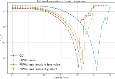
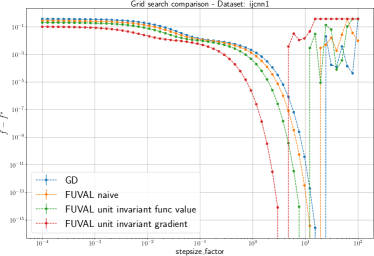
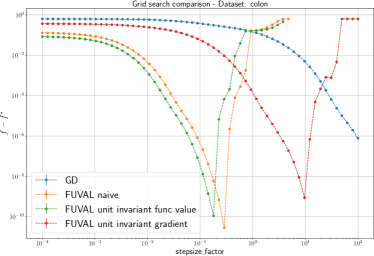
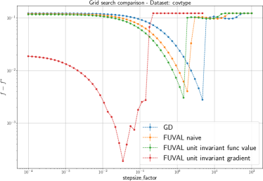
Figure 1: Comparing GD vs. full batch FUVAL in terms of sensitivity to their only tunable parameter: $c$ for FUVAL and stepsize for GD.

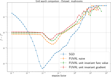
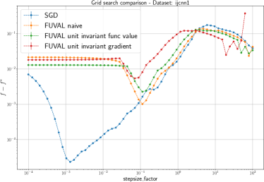
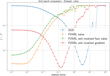
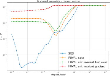
Figure 2: Comparing SGD vs. FUVAL in terms of sensitivity to their only tunable parameter: $c$ for FUVAL and stepsize for SGD.

Appendix A Auxiliary Lemmas

This following lemma is taken from Proposition 3 in [KR20].

Lemma A.1 (Smoothness inequality).

Let $f_{i}:\mathbb{R}^{d}\to\mathbb{R}$ be $L_{i}$–smooth and bounded from below, and let $L_{\max}=\displaystyle\max_{i=1,\ldots,n}L_{i}$. Then, for all $w\in\mathbb{R}^{d}$ and $i=1,\dots,n$ it holds

$$f_{i}(w)-\inf f_{i}\geq\frac{1}{2L_{i}}\left\|\nabla f_{i}(w)\right\|^{2}\enspace.$$ (49)

Consequently, if $i\sim\frac{1}{n}$ then taking expectation we have that for any $w\in\mathbb{R}^{d}$ it holds

$$\mathbb{E}\left[\left\|\nabla f_{i}(w)\right\|^{2}\right]\leq 2L_{\max}(f(w)-\inf f+\inf f-\mathbb{E}\left[\inf f_{i}\right])\enspace.$$ (50)

If all $f_{i}$ are additionally convex, and if $w^{*}\in\operatorname{argmin}f(w)$, then

$$f(w)-f(w^{*})=\mathbb{E}\left[f_{i}(w)-f_{i}(w^{*})\right]\geq\frac{1}{2L_{\max}}\mathbb{E}\left[\left\|\nabla f_{i}(w)-\nabla f_{i}(w^{*})\right\|^{2}\right]\enspace.$$ (51)

Proof.

Using Lemma 5.7 in [Bec17] for $f_{i}$ , we obtain that for all $u,w\in\mathbb{R}^{d}$ it holds

$$\inf f_{i}\leq f_{i}(u)\leq f_{i}(w)+\langle\nabla f_{i}(v),u-w\rangle+\frac{L_{i}}{2}\|u-w\|^{2}.$$

Minimizing the right-hand side over $u$, the minimum is attained at $\hat{u}=w-\frac{1}{L_{i}}\nabla f_{i}(w)$. Plugging in yields

$$\inf f_{i}\leq f_{i}(w)-\langle\nabla f_{i}(w),\frac{1}{L_{i}}\nabla f_{i}(w)\rangle+\frac{L_{i}}{2}\|\frac{1}{L_{i}}\nabla f_{i}(w)\|^{2}=f_{i}(w)-\frac{1}{2L_{i}}\|\nabla f_{i}(w)\|^{2}.$$

Using that $L_{i}\leq L_{\max}$ for all $i=1,\dots,n$, we have $\|\nabla f_{i}(w)\|^{2}\leq 2L_{\max}(f_{i}(w)-\inf f_{i})$. To prove (50), we simply add and subtract $\inf f$ then take expectation and note that $\mathbb{E}\left[f_{i}(w)\right]=f(w)$.
Finally in order to proof (51), by assumption $f_{i}$ is convex and $L_{\max}$–smooth. Applying inequality (2.1.10) of Theorem 2.1.5 in [Nes13] for $f_{i}$ and substituting $x\leftarrow w^{*}$ and $y\leftarrow w$, we obtain

$$f_{i}(w)-f_{i}(w^{*})\geq\left<\nabla f_{i}(w^{*}),w-w^{*}\right>+\frac{1}{2L_{\max}}\left\|\nabla f_{i}(w)-\nabla f_{i}(w^{*})\right\|^{2}.$$

Taking expectation and using that

$$\mathbb{E}\left[\left<\nabla f_{i}(w^{*}),w-w^{*}\right>\right]=\left<\nabla f(w^{*}),w-w^{*}\right>=0,$$

give the result (51). ∎

Lemma A.2.

Let $y,a\in\mathbb{R}^{p}$ and $c\in\mathbb{R}$. The solution to

$$y^{+}=\arg\min_{y}\Big{(}c+\langle a,y-y^{0}\rangle\Big{)}_{+}+\frac{1}{2\beta}\|y-y^{0}\|^{2}$$

is given by

$$y^{+}=y^{0}-\min\big{\{}\beta,\frac{(c)_{+}}{\|a\|^{2}}\big{\}}a.$$

Proof.

See Proposition 3 in [BZK20]. ∎

Lemma A.3 (Projection Inequality Constraint).

Let $c\in\mathbb{R}$ and $w,w^{0},a\in\mathbb{R}^{d}$ . The closed form solution to

$$w^{\prime}= \operatorname{argmin}_{w\in\mathbb{R}^{d}}\left\|w-w^{0}\right\|^{2}$$

$$\,\mbox{subject to }a^{\top}(w-w^{0})+c\leq 0\enspace,$$ (52)

is given by

$$w^{\prime} =w^{0}-\frac{(c)_{+}}{\left\|a\right\|^{2}}a,$$ (53)

where we denote $(x)_{+}=\begin{cases}x&\mbox{ if }x\geq 0\\ 0&\mbox{otherwise}\end{cases}.$

Proof.

If $c\leq 0$ then clearly $w=w^{0}$ is the solution. Otherwise, the solution is given by projecting onto the affine space $a^{\top}(w-w^{0})+c=0.$ The solution to this projection is given by the pseudoinverse, that is

$$w^{\prime}=w^{0}-ca^{\dagger}=w^{0}-\frac{c}{\left\|a\right\|^{2}}a.\qed$$

∎

Lemma A.4 (Projection Inequality Constraint with slack).

Let $\delta>0,c\in\mathbb{R}$ and $w,w^{0},a\in\mathbb{R}^{d}$ . The closed form solution to

$$w^{\prime},s^{\prime}= \operatorname{argmin}_{w\in\mathbb{R}^{d},s\in\mathbb{R}}\left\|w-w^{0}\right\|^{2}+\delta(s-s^{0})^{2}$$

$$\,\mbox{subject to }a^{\top}(w-w^{0})+c\leq s\enspace,$$ (54)

is given by

$$w^{\prime} =w^{0}-\delta\frac{(c-s^{0})_{+}}{1+\delta\left\|a\right\|^{2}}a,$$ (55)

$$s^{\prime} =s^{0}+\frac{(c-s^{0})_{+}}{1+\delta\left\|a\right\|^{2}},$$ (56)

where we denote $(x)_{+}=\begin{cases}x&\mbox{ if }x\geq 0\\ 0&\mbox{otherwise}\end{cases}.$

Proof.

The proof is given in Lemma C.2 in [Gow+22]. But for completeness we give an outline of the proof here.

The problem (A.4) is an L2 projection onto a halfspace. The solution depends if the projected vector $(w,s)=(w^{0},s^{0})$ is in the halfspace.

If $w=w^{0}$ and $s=s^{0}$ satisfies in the linear inequality constraint, that is if $c\leq s^{0}$, in which case the solution is simply $w^{\prime}=w^{0}$ and $s^{\prime}=s^{0}.$

Else, $(w^{0},s^{0})$ is out of the feasible set, that is $c>s^{0}$, then we need to project $(w^{0},s^{0})$ onto the boundary of the halfspace, which means project onto

$$\{(w,s)\in\mathbb{R}^{d}\times\mathbb{R}^{d}\,|\,a^{\top}(w-w^{0})+c=s\}\enspace.$$

In which case the solution is given in by the equality constrained version

$$w^{\prime},s^{\prime}= \operatorname{argmin}_{w\in\mathbb{R}^{d},s\in\mathbb{R}^{b}}\left\|w-w^{0}\right\|^{2}+\delta\left\|s-s^{0}\right\|^{2}$$

$$\,\mbox{subject to }a^{\top}(w-w^{0})+c=s\enspace,$$ (57)

which is

$$w^{\prime} =w^{0}-\delta\frac{c-s^{0}}{1+\delta\left\|a\right\|^{2}}a,$$ (58)

$$s^{\prime} =s^{0}+\frac{c-s^{0}}{1+\delta\left\|a\right\|^{2}}.$$ (59)

Combining both cases gives (55)–(56). ∎

Appendix B Missing Proofs

Here we give the missing proofs. All the associated statements are also repeated for ease of reference.

B.1 Proof of Lemma 3.2

See 3.2

Proof.

The proof follows by re-writing the objective function of the projection (33) as

$$s_{j}+\frac{1}{2\lambda}\left\|w-w^{t}\right\|^{2}+\frac{1}{2\delta}(s_{j}-s^{t}_{j})^{2} =\frac{1}{2\lambda}\left\|w-w^{t}\right\|^{2}+\frac{1}{2\delta}(s_{j}-s^{t}_{j}+\delta)^{2}+\mbox{constants}.$$

Thus we can re-write the projection (33) as

$$w^{t+1},s^{t+1}= \underset{w\in\mathbb{R}^{d},s_{j}\in\mathbb{R}^{n}}{\rm{argmin}}~{}\left\|w-w^{t}\right\|^{2}+\frac{\lambda}{\delta}(s_{j}-(s_{j}^{t}-\delta))^{2}+\frac{\lambda}{\delta}\sum_{i\neq j}(s_{i}-s_{i}^{t})^{2}$$

$$\mbox{ subject to }f_{j}(w^{t})+\left<\nabla f_{j}(w^{t}),w-w^{t}\right>\leq s_{j},$$ (60)

This projection is now separable in the slack variables $s_{i}$ for $i\neq j.$ Indeed, for these slack variables the solution is simply $s_{i}^{t+1}=s_{i}^{t}$ for every $i\neq j.$

Consequently we can now apply Lemma A.4 where $\delta\leftarrow\frac{\lambda}{\delta}$ and $s^{0}\leftarrow s^{t}-\delta$, which gives the solution

$$w^{t+1} =w^{t}-\lambda\frac{(f_{j}(w^{t})-s_{j}^{t}+\delta)_{+}}{\delta+\lambda\left\|\nabla f_{j}(w^{t})\right\|^{2}}\nabla f_{j}(w^{t})$$ (61)

$$s_{j}^{t+1} =s_{j}^{t}-\delta+\delta\frac{(f_{j}(w^{t})-s_{j}^{t}+\delta)_{+}}{\delta+\lambda\left\|\nabla f_{j}(w^{t})\right\|^{2}}.$$ (62)

∎

B.2 Proof of Lemma 3.3

See 3.3

Proof.

first note that if $f_{i}$ are assumed to be convex, then (37) is a convex problem, as $(\cdot)_{+}$ is nondecreasing and convex. We derive the necessary first-order optimality conditions of (37) (cf. [Bec17, Thm. 3.63]). For $(w,s)$, they are

$$u_{i} \in\partial(f_{i}(w)-s_{i})_{+},\quad i=1,\dots,n,$$ (63)

$$0 \in\frac{1}{n}\sum_{i=1}^{n}cu_{i}\partial f_{i}(w),$$ (64)

$$0 =1-cu_{i},\quad i=1,\dots,n.$$ (65)

Here, we used the fact that $(f_{i}(w)-s_{i})_{+}=\max\{f_{i}(w)-s_{i},0\}$ is the pointwise maximum of convex functions and applied [HUL01, Cor. 4.3.2]. We do a simple case distinction:

1. If $s_{i}>f_{i}(w)$, then $\partial(f_{i}(w)-s_{i})_{+}=\{0\}$. In this case, (65) cannot be fulfilled.

2. If $s_{i}<f_{i}(w)$, then $\partial(f_{i}(w)-s_{i})_{+}=\{1\}$. From (65) we have $u_{i}=1/c$ which implies $c=1$.

3. If $s_{i}=f_{i}(w)$, then $\partial(f_{i}(w)-s_{i})_{+}=[0,1]$. From (65) we have $u_{i}=1/c$ which implies $c\geq 1$.

At any solution $(w^{*},s^{*})$, the necessary first-order optimality conditions are fulfilled and hence it must hold $s_{i}^{*}\leq f_{i}(w^{*})$ for all $i\in[n]$. Plugging (65) into (64) gives $0\in\frac{1}{n}\sum_{i=1}^{n}\partial f_{i}(w^{*})$ and hence $0\in\partial f(w^{*})$. Hence, $w^{*}$ is a (global) minimum of $f$ (due to convexity). Moreover, as $s_{i}^{*}\leq f_{i}(w^{*})$ and $c\geq 1$, we have

$$g(w^{*},s^{*})=\frac{1}{n}\sum_{i=1}^{n}s_{i}^{*}+c(f_{i}(w^{*})-s_{i}^{*})_{+}=\frac{1}{n}\sum_{i=1}^{n}(1-c)s_{i}^{*}+cf_{i}(w^{*}).$$

Now, we either have $s_{i}^{*}<f_{i}(w^{*})$ in which case $c=1$ and hence

$$(1-c)s_{i}^{*}+cf_{i}(w^{*})=f_{i}(w^{*}).$$

Otherwise, $c>1$, but then $s_{i}^{*}=f_{i}(w^{*})$ from (65) and hence $(1-c)s_{i}^{*}+cf_{i}(w^{*})=f_{i}(w^{*})$. Altogether, we get $g(w^{*},s^{*})=f(w^{*})$. ∎

B.3 Proof of Lemma 3.5

See 3.5

Proof.

Introducing the variables $\hat{s}:=\sqrt{\frac{\lambda_{t}}{\delta_{t}}}s$ and hence $\hat{s}^{t}:=\sqrt{\frac{\lambda_{t}}{\delta_{t}}}s^{t}$, problem (40) is equivalent to

$$w^{t+1},\hat{s}^{t+1}=\operatorname{argmin}_{w,\hat{s}}\sqrt{\frac{\delta_{t}}{\lambda_{t}}}\hat{s}_{j_{t}} +c\Big{(}f_{j_{t}}(w^{t})+\langle\nabla f_{j_{t}}(w^{t}),w-w^{t}\rangle-\sqrt{\frac{\delta_{t}}{\lambda_{t}}}\hat{s}_{j_{t}}\Big{)}_{+}$$

$$+\frac{1}{2\lambda_{t}}\|w-w^{t}\|^{2}+\frac{1}{2\lambda_{t}}\|\hat{s}-\hat{s}^{t}\|^{2}.$$ (66)

Denote $\nu_{t}:=\sqrt{\delta_{t}/\lambda_{t}}$. Completing the squares gives

$$\nu_{t}\hat{s}_{i}+\frac{1}{2\lambda_{t}}(\hat{s}_{i}-\hat{s}_{i}^{t})^{2}=\frac{1}{2\lambda_{t}}(\hat{s}_{i}-\hat{s}_{i}^{t}+\sqrt{\lambda_{t}\delta_{t}})^{2}+\mathrm{constants}(\hat{s}_{i}),$$

and hence

$$w^{t+1},\hat{s}^{t+1}= \operatorname{argmin}_{w,\hat{s}}c\Big{(}f_{j_{t}}(w^{t})+\langle\nabla f_{j_{t}}(w^{t}),w-w^{t}\rangle-\nu_{t}\hat{s}_{j_{t}}\Big{)}_{+}+\frac{1}{2\lambda_{t}}\|w-w^{t}\|^{2}+\frac{1}{2\lambda_{t}}(\hat{s}_{j_{t}}-(\hat{s}_{j_{t}}^{t}-\sqrt{\lambda_{t}\delta_{t}}))^{2},$$

$$\text{subject to }\hat{s}_{i}=\hat{s}_{i}^{t},\quad i\neq j_{t}.$$

Applying Lemma A.2 with

$$y^{0}=\begin{bmatrix}w^{t}\\ \hat{s}_{j_{t}}^{t}-\sqrt{\lambda_{t}\delta_{t}}\end{bmatrix},~{}\beta=c\lambda_{t},~{}a=\begin{bmatrix}\nabla f_{j_{t}}(w^{t})\\ -\nu_{t}\end{bmatrix},~{}c=f_{j_{t}}(w^{t})-\nu_{t}\hat{s}_{j_{t}}^{t}+\sqrt{\lambda_{t}\delta_{t}}\nu_{t}$$

gives the update

$$\hat{\tau}_{t} :=\min\Big{\{}\lambda_{t}c,\frac{\big{(}f_{j_{t}}(w^{t})-\nu_{t}\hat{s}_{j_{t}}^{t}+\delta_{t}\big{)}_{+}}{\|\nabla f_{j_{t}}(w^{t})\|^{2}+\nu_{t}^{2}}\Big{\}},$$

$$w^{t+1} =w^{t}-\hat{\tau}_{t}\nabla f_{j_{t}}(w^{t}),$$

$$\hat{s}^{t+1}_{j} =\hat{s}_{j}^{t}-\sqrt{\lambda_{t}\delta_{t}}+\hat{\tau}_{t}\nu_{t},\quad\text{if }j=j_{t},$$

$$\hat{s}^{t+1}_{j} =\hat{s}_{j}^{t},\quad\text{if }j\neq j_{t},$$

where we used that $\sqrt{\lambda_{t}\delta_{t}}\nu_{t}=\delta_{t}$. Substituting back $s^{t}:=\nu_{t}\hat{s}^{t}$ and using $\nu_{t}=\sqrt{\delta_{t}/\lambda_{t}}$ and $\hat{\tau}_{t}=\lambda_{t}\tau_{t}$ gives the solution (42). ∎

B.4 Proof of Lemma 3.6

See 3.6

Proof.

Using again the substitution $s^{t}:=\sqrt{\frac{\delta_{t}}{\lambda_{t}}}\hat{s}^{t}=\sqrt{\frac{\delta}{\lambda}}\hat{s}^{t}$ and returning to (66) have again that

$$w^{t+1},\hat{s}^{t+1}=\operatorname{argmin}_{w,\hat{s}}\sqrt{\frac{\delta}{\lambda}}\hat{s}_{j_{t}} +c\Big{(}f_{j_{t}}(w^{t})+\langle\nabla f_{j_{t}}(w^{t}),w-w^{t}\rangle-\sqrt{\frac{\delta}{\lambda}}\hat{s}_{j_{t}}\Big{)}_{+}$$

$$+\frac{1}{2\lambda_{t}}\|w-w^{t}\|^{2}+\frac{1}{2\lambda_{t}}\|\hat{s}-\hat{s}^{t}\|^{2}.$$ (67)

Multiplying the objective by $\sqrt{\frac{\lambda}{\delta}}$ and defining $\hat{f}_{j}=\sqrt{\frac{\lambda}{\delta}}f_{j}$ and $\rho_{t}:=\sqrt{\frac{\delta}{\lambda}}\lambda_{t}=\frac{\sqrt{\lambda\delta}}{\sqrt{t+1}}$ gives

$$w^{t+1},\hat{s}^{t+1}=\operatorname{argmin}_{w,\hat{s}}\hat{s}_{j_{t}} +c\Big{(}\hat{f}_{j_{t}}(w^{t})+\langle\nabla\hat{f}_{j_{t}}(w^{t}),w-w^{t}\rangle-\hat{s}_{j_{t}}\Big{)}_{+}$$

$$+\frac{1}{2\rho_{t}}\|w-w^{t}\|^{2}+\frac{1}{2\rho_{t}}\|\hat{s}-\hat{s}^{t}\|^{2}.$$ (68)

The above is now the model-based method Algorithm 2 with step size $\rho_{t}$ applied to minimizing

$$\min_{w\in\mathbb{R}^{d},\hat{s}\in\mathbb{R}^{n}}\frac{1}{n}\sum_{i=1}^{n}\Big{(}\hat{s}_{i}+c(\hat{f}_{i}(w)-\hat{s}_{i})_{+}\Big{)}.$$ (69)

Since $f_{i}$ is $G_{i}$–Lipschitz, we have that $\hat{f}_{i}$ is $\sqrt{\frac{\lambda}{\delta}}G_{i}$–Lipschitz. Consequently by Lemma C.2 the model is

$$\hat{M}_{i}:=\big{(}1+c\sqrt{\frac{\lambda}{\delta}G_{i}^{2}+1}\big{)}$$

Lipschitz. Let $\hat{\mathsf{M}}\coloneqq\sqrt{\tfrac{1}{n}\sum_{i=1}^{n}\hat{M}_{i}^{2}}.$ Since $\rho_{t}=\frac{\sqrt{\lambda\delta}}{\sqrt{t+1}}=:\frac{\rho}{\sqrt{t+1}},$ we have by Corollary C.6 we have the following convergence

$$\mathbb{E}\Big{[}\hat{f}(\bar{w}^{T})-\hat{f}(w^{*})\Big{]}\leq\frac{\|w^{0}-w^{*}\|^{2}+\|\hat{s}^{0}-\hat{s}^{*}\|^{2}}{4\rho(\sqrt{T+2}-1)}+\frac{\hat{\mathsf{M}}^{2}\rho(1+\ln(T+1))}{2\sqrt{T+2}-2}.$$ (70)

Substituting back $s^{t}=\sqrt{\frac{\delta}{\lambda}}\hat{s}^{t}$, $f=\sqrt{\frac{\delta}{\lambda}}\hat{f}$ and $\rho=\sqrt{\delta\lambda}$ gives (43).

∎

B.5 Proof of Lemma 3.7

See 3.7

Proof.

Since both $f$ and $\phi_{t}$ are convex, their minimizers are exactly their critical points. The gradient of $\phi_{i,t}$ is given by

$$\nabla\phi_{i,t}(w,s)=\frac{(f_{i}(w)-s_{i}+\delta)_{+}}{\delta+\lambda\|\nabla f_{i}(w^{t})\|^{2}}\begin{pmatrix}\nabla f_{i}(w)\\ -e_{i}\end{pmatrix}+\begin{pmatrix}0\\ e_{i}\end{pmatrix}$$ (71)

where $e_{j}\in\mathbb{R}^{n}$ denotes the $j$-th vector of the canonical basis. Let $(w^{*},s^{*}_{t})$ be a critical point of $\phi_{t}$ (45) and thus satisfying

$$\frac{1}{n}\sum_{i=1}^{n}\frac{(f_{i}(w^{*})-(s^{*}_{t})_{i}+\delta)_{+}}{\delta+\lambda\|\nabla f_{i}(w^{t})\|^{2}}\nabla f_{i}(w^{*}) =0,$$ (72)

$$\frac{(f_{i}(w^{*})-(s^{*}_{t})_{i}+\delta)_{+}}{\delta+\lambda\|\nabla f_{i}(w^{t})\|^{2}} =1,\quad\mbox{for }j=1,\ldots,n.$$ (73)

Inserting the second row of the above into the first gives

$$\frac{1}{n}\sum_{i=1}^{n}\nabla f_{i}(w^{*})=0.$$ (74)

Consequently $w^{*}$ is a critical point of $f$.

Now let $w^{*}$ be a critical point of $f$. By choosing $s_{i,t}^{*}$ given in (46) it easy to see that (73) holds. Consequently, plugging (73) into (72) and using  (74), we conclude that $(w^{*},s^{*}_{t})$ is a critical point of $\phi_{t}$. ∎

B.6 Proof of Lemma 3.8

See 3.8

Proof.

Recall (71). Therefore,

$$\nabla_{w}\phi_{j_{t},t}(w^{t},s^{t}) =\tau_{t}\nabla f_{j_{t}}(w^{t})$$

$$\nabla_{s_{j_{t}}}\phi_{j_{t},t}(w^{t},s^{t}) =1-\tau_{t},\mbox{ and, }$$

$$\nabla_{s_{i}}\phi_{j_{t},t}(w^{t},s^{t}) =0,\quad\mbox{ for }i\neq j_{t}.$$

Plugging the above gradients into (47) gives (44). ∎

B.7 Proof of Theorem 3.9

See 3.9

Proof.

Denote $z^{t}=(w^{t},s^{t})$. Consider the estimate (97) in Lemma D.10, together with the notation $\bar{\sigma}_{t}^{*}$ in (99). Reordering the terms in (97), summing both sides for $t=0,\ldots,T-1$ and dividing by $T$ we have (after cancellations due to a telescopic sum of positive terms) that

$$\frac{2\gamma(1-\gamma)}{T}\sum\limits_{t=0}^{T-1}\mathbb{E}[\phi_{t}(z^{t})-\phi_{t}(z^{*})]\leq\frac{1}{T}\mathbb{E}[\left\|z^{0}-z^{*}\right\|^{2}_{{\bf D}}]+\frac{2\gamma^{2}}{T}\sum\limits_{t=0}^{T-1}\bar{\sigma}_{t}^{*}.$$ (75)

Consider now that $w^{*}\in{\rm{argmin}}~{}f$ and $s_{i}^{*}=f_{i}(w^{*})$. In particular, from Lemma D.10 we have that $\bar{\sigma}_{t}^{*}\leq\sigma$. Moreover, from the definition of $\phi_{t}$ in (45) is easy to see that $\phi_{t}(z^{*})\leq\inf f+\frac{\delta}{2}$. Furthermore using Lemma D.6 we have that

$$\phi_{t}(z^{t})\geq\inf f+\frac{\delta}{2}-\lambda L_{\max}\sigma+(1-\lambda L_{\max})(f(w^{t})-\inf f).$$

Using these observations in (75) we have

$$\frac{2\gamma(1-\gamma)}{T}\sum\limits_{t=0}^{T-1}\mathbb{E}[(1-\lambda L_{\max})(f(w^{t})-\inf f)-\lambda L_{\max}\sigma]\leq\frac{1}{T}\mathbb{E}[\left\|z^{0}-z^{*}\right\|_{{\bf D}}^{2}]+{2\gamma^{2}}\sigma.$$

Reordering the terms, and using Jensen inequality, we get

$${2\gamma(1-\gamma)(1-\lambda L_{\max})}\mathbb{E}[f(\bar{w}^{T})-\inf f]\leq\frac{1}{T}\mathbb{E}[\left\|z^{0}-z^{*}\right\|_{{\bf D}}^{2}]+2\gamma\sigma(\gamma+\lambda L_{\max}(1-\gamma)).$$

Use the fact that $\gamma<1$ and $2\lambda L_{\max}<1$ so that we can divide by nonzero constants, and finally obtain

$$\mathbb{E}[f(\bar{w}^{T})-\inf f]\leq\frac{1}{2\gamma(1-\gamma)(1-\lambda L_{\max})T}\mathbb{E}[\left\|z^{0}-z^{*}\right\|_{{\bf D}}^{2}]+\sigma\frac{\gamma+\lambda L_{\max}(1-\gamma)}{(1-\gamma)(1-\lambda L_{\max})}.$$

∎

Appendix C Prox-linear as a Model Based Method

Here we clarify the connection between the method (42) and the prox-linear method. To do so, we adopt much of the notation of model based methods [DD19]. We then show how to adapt the results given in [DD19] to our setting.

Define $h_{i}:\mathbb{R}^{2}\to\mathbb{R}$ and $c_{i}:\mathbb{R}^{d+n}\to\mathbb{R}^{2}$ as follows: for $z=(z_{1},z_{2})\in\mathbb{R}^{2}$, and $u=(w,s)\in\mathbb{R}^{d+n}$ let

$$h_{i}(z) :=z_{2}+c(z_{1})_{+},$$

$$c_{i}(w,s) :=\begin{bmatrix}f_{i}(w)-s_{i}\\ s_{i}\end{bmatrix}.$$

In a slight abuse of notation, we will write both $c_{i}(u)$ and $c_{i}(w,s)$ interchangeably when $u=(w,s)$. With the above, (37) is equivalent to the problem

$$\min_{(w,s)\in\mathbb{R}^{d+n}}\frac{1}{n}\sum_{i=1}^{n}h_{i}(c_{i}(w,s)).$$ (76)

Let us define the objective function of (76) as

$$g(w,s):=\frac{1}{n}\sum_{i=1}^{n}h_{i}(c_{i}(w,s)).$$

In the philosophy of mode-based stochastic proximal point [DD19], we construct the prox-linear model of the objective function: for $u=(w,s)\in\mathbb{R}^{d+n}$ and $y=(v,q)\in\mathbb{R}^{d+n}$, define

$$\begin{split}g_{u}(y;i):&=h_{i}\big{(}c_{i}(u)+\langle\nabla c_{i}(u),y-u\rangle\big{)}\\ &=q_{i}+c\big{(}f_{i}(w)+\langle\nabla f_{i}(w),v-w\rangle-q_{i}\big{)}_{+}.\end{split}$$ (77)

In iteration $t$, if $j_{t}\in[n]$ is drawn at random, the model-based update is given by

$$u^{t+1}=\arg\min_{u}h_{j_{t}}(c_{j_{t}}(u^{t})+\langle\nabla c_{j_{t}}(u^{t}),u-u^{t}\rangle)+\frac{1}{2\lambda_{t}}\|u-u^{t}\|^{2},$$

where $\lambda_{t}>0$ is the step size. Rewriting in terms of $u^{t}=(w^{t},s^{t})$ and plugging in the definition of $h_{i},c_{i}$ we have (78).

$$w^{t+1},s^{t+1}=\arg\min_{w,s}s_{j_{t}}+c\Big{(}f_{j_{t}}(w^{t})+\langle\nabla f_{j_{t}}(w^{t}),w-w^{t}\rangle-s_{j_{t}}\Big{)}_{+}+\frac{1}{2\lambda_{t}}\Big{(}\|w-w^{t}\|^{2}+\|s-s^{t}\|^{2}\Big{)}.$$ (78)

We now give a closed-form solution for the iterate update (78).

Lemma C.1.

The solution to (78) is given by

$$\tau_{t} :=\min\Big{\{}\lambda_{t}c,\frac{\big{(}f_{j_{t}}(w^{t})-s_{j_{t}}^{t}+\lambda_{t}\big{)}_{+}}{\|\nabla f_{j_{t}}(w^{t})\|^{2}+1}\Big{\}},$$

$$w^{t+1} =w^{t}-\tau_{t}\nabla f_{j_{t}}(w^{t}),$$

$$s^{t+1}_{j} =s_{j}^{t}-\lambda_{t}+\tau_{t},\quad\text{if }j=j_{t},$$

$$s^{t+1}_{j} =s_{j}^{t},\quad\text{if }j\neq j_{t}.$$

Proof.

For any $i$, we have $s_{i}+\frac{1}{2\lambda_{t}}(s_{i}-s_{i}^{t})^{2}=\frac{1}{2\lambda_{t}}(s_{i}-s_{i}^{t}+\lambda_{t})^{2}+s_{i}^{t}-\frac{\lambda_{t}}{2}$. Note that $s_{i}^{t}-\frac{\lambda_{t}}{2}$ is constant in $w,s$. Thus, problem (78) is equivalent to solving

$$w^{t+1},s^{t+1}= \arg\min_{w,s}c\Big{(}f_{j_{t}}(w^{t})+\langle\nabla f_{j_{t}}(w^{t}),w-w^{t}\rangle-s_{j_{t}}\Big{)}_{+}+\frac{1}{2\lambda_{t}}\Big{(}\|w-w^{t}\|^{2}+(s_{j_{t}}-(s^{t}_{j_{t}}-\lambda_{t}))^{2}\Big{)}$$

$$\text{subject to}\quad s_{j}=s_{j}^{t},\quad j\neq j_{t}.$$

Dividing by $c$ and applying Lemma A.2 with $y^{0}=(w^{t},s_{j_{t}}^{t}-\lambda_{t})$, $a=(\nabla f_{j_{t}}(w^{t}),-1)$, $\beta=\lambda_{t}c$ and $c=f_{j_{t}}(w^{t})-s_{j_{t}}^{t}+\lambda_{t}$, we get the claimed update. ∎

We next show properties of the model function $g_{u}(y;i)$.

Lemma C.2.

Let $P$ be the uniform probability measure on $\{1,\dots,n\}$, i.e. $P(\{i\})=\frac{1}{n}$ for all $i\in[n]$. Let further $u=(w,s)\in\mathbb{R}^{d+n}$ and $y=(v,q)\in\mathbb{R}^{d+n}$. For $i\in[n]$ recall

$$g_{u}(y;i)=h_{i}(c_{i}(u)+\langle\nabla c_{i}(u),y-u\rangle)=q_{i}+c\big{(}f_{i}(w)+\langle\nabla f_{i}(w),v-w\rangle-q_{i}\big{)}_{+}.$$

Then, it holds:

1. It is possible to generate i.i.d. realizations $j_{1},j_{2},\dots\sim P$.

2. We have $\mathbb{E}_{j\sim P}[g_{u}(u;j)]=\frac{1}{n}\sum_{i=1}^{n}g_{u}(u;i)=g(w,s)$ for all $u\in\mathbb{R}^{d+n}$. Further, if $f_{i}$ is convex for all $i\in[n]$, then

   $$\mathbb{E}_{j\sim P}[g_{u}(y;j)]=\frac{1}{n}\sum_{i=1}^{n}g_{u}(y;i)\leq g(v,q)\quad\forall u,y\in\mathbb{R}^{d+n}.$$

3. The mapping $y\mapsto g_{u}(y;i)$ is convex for all $u$ and all $i\in[n]$.

4. If $f_{i}$ is $G_{i}$-Lipschitz for all $i\in[n]$, define $M_{i}:=\big{(}1+c\sqrt{G_{i}^{2}+1}\big{)}$ and $\mathsf{M}:=\sqrt{\frac{1}{n}\sum_{i=1}^{n}M_{i}^{2}}$. Then,

   $$g_{u}(u;i)-g_{u}(y;i)\leq M_{i}\|u-y\|\quad\forall u,y\in\mathbb{R}^{d+n}.$$

Proof.

1. Evident.

2. The first statement follows immediately from the definition of $g_{u}(\cdot;i)$ and $g$. For the second statement, due to convexity of $f_{i}$ we have

   $$c_{i}(u)+\langle c_{i}(u),y-u\rangle=\begin{bmatrix}f_{i}(w)+\langle\nabla f_{i}(w),v-w\rangle-q_{i}\\ q_{i}\end{bmatrix}\overset{\text{componentwise}}{\leq}\begin{bmatrix}f_{i}(v)-q_{i}\\ q_{i}\end{bmatrix}=c_{i}(y).$$

   Since $h_{i}$ is monotone in each component, we get

   $$g_{u}(y;i)=h_{i}(c_{i}(u)+\langle c_{i}(u),y-u\rangle)\leq h_{i}(c_{i}(y)).$$

   Summing over $=1,\dots,n$ and dividing by $n$ gives the result.

3. The function $h_{i}$ is convex as $(\cdot)_{+}$ is convex. The function $y\mapsto g_{u}(y;i)$ is a composition of a convex and a linear mapping and therefore convex.

4. Denote with $e_{i}$ the $i$-t element of the standard Euclidean basis. Using $(a)_{+}-(b)_{+}\leq(a-b)_{+}$ we have

   $$g_{u}(u;i)-g_{u}(y;i) =s_{i}+c\big{(}\underbrace{f_{i}(w)-s_{i}}_{=:a}\big{)}_{+}-q_{i}-c\big{(}\underbrace{f_{i}(w)+\langle\nabla f_{i}(w),v-w\rangle-q_{i}}_{=:b}\big{)}_{+}$$

   $$\leq s_{i}-q_{i}+c\big{(}\langle\nabla f_{i}(w),w-v\rangle+q_{i}-s_{i}\big{)}_{+}$$

   $$=s_{i}-q_{i}+c\Big{(}[\nabla f_{i}(w),-e_{i}]^{T}\begin{bmatrix}w-v\\ s-q\end{bmatrix}\Big{)}_{+}$$

   $$\leq s_{i}-q_{i}+c\|[\nabla f_{i}(w),-e_{i}]\|\cdot\|y-u\|\leq\big{(}1+c\|[\nabla f_{i}(w),-e_{i}]\|\big{)}\|y-u\|.$$

   With $\|[\nabla f_{i}(w),-e_{i}]\|=\sqrt{\|\nabla f_{i}(w)\|^{2}+1}\leq\sqrt{G_{i}^{2}+1}$, we conclude

   $$g_{u}(u;i)-g_{u}(y;i)\leq\big{(}1+c\sqrt{G_{i}^{2}+1}\big{)}\|y-u\|\quad\forall x,y.$$

∎

Corollary C.3.

Let $f_{i}$ be convex and $G_{i}$-Lipschitz for all $i\in[n]$. Then, $g_{u}(y;i)$ is a stochastic one-sided model in the sense of [DD19, Assum. B].

Proof.

The statements (B1)-(B4) in Lemma C.2 coincide with (B1)-(B4) in [DD19, Assum. B] for (in the notation of [DD19]) $r=0$, and $\tau=\eta=0$, $\mathsf{L}=\mathsf{M}$. ∎

C.1 Convergence analysis

1:Inputs: step sizes $\lambda_{t}>0,$ penalty multiplier $c\geq 1$.

2:Initialize: $w^{0}\in\mathbb{R}^{d}$ and $s_{i}^{0}\in\mathbb{R}$ for $i=1,\ldots,n.$

3:for $t=0,\ldots,T$ do

4:     Sample $j_{t}$ randomly from $[n]$.

5:     Compute $\tau_{t}=\min\Big{\{}\lambda_{t}c,\frac{\big{(}f_{j_{t}}(w^{t})-s_{j_{t}}^{t}+\lambda_{t}\big{)}_{+}}{\|\nabla f_{j_{t}}(w^{t})\|^{2}+1}\Big{\}}$ and update

6:     $\displaystyle w^{t+1}\;=w^{t}-\tau_{t}\nabla f_{j_{t}}(w^{t})$

7:     $\displaystyle s^{t+1}_{i}\;=\begin{cases}s_{i}^{t}-\lambda_{t}+\tau_{t},\quad&\text{if }i=j_{t},\\ s_{i}^{t},\quad&\text{else.}\end{cases}$

8:Output: $w^{T+1},s^{T+1}$

Algorithm 2

Proposition C.4.

Let $f_{i}$ be convex and $G_{i}$-Lipschitz for all $i\in[n]$. Let $(w^{*},s^{*})\in\operatorname{argmin}_{w,s}g(w,s)$. Let the iterates $(w^{t},s^{t})$ be generated by Algorithm 2 with step sizes $\lambda_{t}>0$. Then, it holds

$$2\lambda_{t}\mathbb{E}\Big{[}g(w^{t+1},s^{t+1})-g(w^{*},s^{*})\Big{]}\leq\mathbb{E}\|(w^{t},s^{t})-(w^{*},s^{*})\|^{2}-\mathbb{E}\|(w^{t+1},s^{t+1})-(w^{*},s^{*})\|^{2}+2\mathsf{M}^{2}\lambda_{t}^{2}.$$ (79)

Define $\bar{w}^{T}:=\frac{1}{T+1}\sum_{t=0}^{T}\lambda_{t}w^{t+1}$ and $\bar{s}^{T}:=\frac{1}{T+1}\sum_{t=0}^{T}\lambda_{t}s^{t+1}$. Choosing $\lambda_{t}=\frac{\lambda}{\sqrt{t+1}}$, for some $\lambda>0$, we have

$$\mathbb{E}\Big{[}g(\bar{w}^{T},\bar{s}^{T})-g(w^{*},s^{*})\Big{]}\leq\frac{\|w^{0}-w^{*}\|^{2}+\|s^{0}-s^{*}\|^{2}}{4\lambda(\sqrt{T+2}-1)}+\frac{\mathsf{M}^{2}\lambda(1+\ln(T+1))}{2\sqrt{T+2}-2}.$$ (80)

Choosing $\lambda_{t}=\frac{\lambda}{\sqrt{T+1}}$ instead, we get

$$\mathbb{E}\Big{[}g(\bar{w}^{T},\bar{s}^{T})-g(w^{*},s^{*})\Big{]}\leq\frac{\|w^{0}-w^{*}\|^{2}+\|s^{0}-s^{*}\|^{2}}{2\lambda\sqrt{T+1}}+\frac{\mathsf{M}^{2}\lambda}{\sqrt{T+1}}=\mathcal{O}(\frac{1}{\sqrt{T+1}}),$$ (81)

Proof.

We apply the theory of [DD19] with $\varphi=g$, $x^{t}=(w^{t},s^{t})$, $\beta_{t}=\lambda_{t}^{-1}$ and $\bar{\rho}=\eta=\tau=0$. Using (4.8) of [DD19, Lem. 4.2] with $x=(w^{*},s^{*})$ and taking expectation yields (79). Now summing (79) from $t=0,\dots,T$ and dividing by $\sum_{t=0}^{T}\lambda_{t}$ yields

$$\tfrac{1}{\sum_{t=0}^{T}\lambda_{t}}\sum_{t=0}^{T}\lambda_{t}\mathbb{E}\Big{[}g(w^{t+1},s^{t+1})-g(w^{*},s^{*})\Big{]}\leq\frac{\|w^{0}-w^{*}\|^{2}+\|s^{0}-s^{*}\|^{2}}{2\sum_{t=0}^{T}\lambda_{t}}+\frac{\mathsf{M}^{2}\sum_{t=0}^{T}\lambda_{t}^{2}}{\sum_{t=0}^{T}\lambda_{t}}.$$ (82)

Using convexity of $g$ and Jensen’s inequality we can estimate the left-hand side from below by $\mathbb{E}\Big{[}g(\bar{w}^{T},\bar{s}^{T})-g(w^{*},s^{*})\Big{]}$. Using the integral bound,

$$\int_{N}^{M+1}h(x)dx\;\leq\;\sum_{n=N}^{M}h(n)\;\leq\;h(N)+\int_{N}^{M}h(x)dx,\quad\mbox{for every decreasing }h(x),\mbox{ and every }N,M\in\mathbb{N},$$

we have that

$$\sum_{t=0}^{T}\tfrac{1}{\sqrt{t+1}}\geq\int_{0}^{T+1}\tfrac{1}{\sqrt{s+1}}ds=2\sqrt{T+2}-2,$$

$$\sum_{t=0}^{T}\tfrac{1}{t+1}\leq 1+\int_{0}^{T}\tfrac{1}{s+1}ds=1+\ln(T+1).$$

Plugging in these estimates gives (80). This same expression (80) is essentially also given in (4.17) of [DD19, Thm. 4.4]. The last claim (81) follows by plugging in $\lambda_{t}=\lambda/\sqrt{T+1}$ into (82). ∎

Now try to connect the values of $f$ and $g$.

Lemma C.5.

Let $c\geq 1$ for all $i\in[n]$ and let $(w,s)\in\mathbb{R}^{d+n}$. Then, it holds $g(w,s)\geq f(w)$.

Proof.

We first show that $s_{i}+c(f_{i}(w)-s_{i})_{+}\geq f_{i}(w)$ for all $i\in[n]$ by case distinction:

1. Assume $f_{i}(w)-s_{i}\leq 0$. Then $(f_{i}(w)-s_{i})_{+}=0$ and

   $$s_{i}+c(f_{i}(w)-s_{i})_{+}=s_{i}\geq f_{i}(w),$$

   where the last inequality follows from the assumption.

2. Assume $f_{i}(w)-s_{i}>0$. Then $s_{i}+c(f_{i}(w)-s_{i})_{+}=(1-c)s_{i}+cf_{i}(w)$. Now $c\geq 1$ implies $1-c\leq 0$ and hence $(1-c)s_{i}\geq(1-c)f_{i}(w)$. Altogether,

   $$s_{i}+c(f_{i}(w)-s_{i})_{+}=(1-c)s_{i}+cf_{i}(w)\geq(1-c)f_{i}(w)+cf_{i}(w)=f_{i}(w).$$

Applying this for all $i\in[n]$, we get

$$g(w,s) =\frac{1}{n}\sum_{i=1}^{n}s_{i}+c(f_{i}(w)-s_{i})_{+}\geq\frac{1}{n}\sum_{i=1}^{n}f_{i}(w)=f(w).$$

∎

Corollary C.6.

Let the assumptions of Proposition C.4 hold. If $c\geq 1$ for all $i\in[n]$, and $\lambda_{t}=\frac{\lambda}{\sqrt{t+1}}$, then we have

$$\mathbb{E}\Big{[}f(\bar{w}^{T})-f(w^{*})\Big{]}\leq\frac{\|w^{0}-w^{*}\|^{2}+\|s^{0}-s^{*}\|^{2}}{4\lambda(\sqrt{T+2}-1)}+\frac{\mathsf{M}^{2}\lambda(1+\ln(T+1))}{2\sqrt{T+2}-2}.$$ (83)

Proof.

As $c\geq 1$ for all $i\in[n]$, we can apply Lemma C.5 to get $f(\bar{w}^{T})\leq g(\bar{w}^{T},\bar{s}^{T})$ almost surely and Lemma 3.3 to get $f(w^{*})=g(w^{*},s^{*})$. Together with (80), we conclude the proof. ∎

Appendix D Convergence Theorem through SGD Viewpoint

In this section we will make use of the following assumptions.

Assumption D.1 (Convexity).

Let $f_{i}$ be convex for all $i\in\{1,\dots,n\}$.

Assumption D.2 (Smoothness).

Let $f_{i}$ be $L_{i}$–Lipschitz smooth for all $i\in\{1,\dots,n\}$, meaning that $\nabla f_{i}$ is $L_{i}$–Lipschitz continuous. Let $L_{\max}:=\max_{i=1,\dots,n}L_{i}$. In this case, $f$ is $L$–Lipschitz smooth for some $L\leq L_{\max}$.

Assumption D.3 (Lipschitz continuity).

Let $f_{i}$ be $G_{i}$–Lipschitz continuous for all $i\in\{1,\dots,n\}$, and define $G^{2}:=\sum_{i}G_{i}^{2}$.

First we prove that each slack variable is lower bounded by the infinum of the function it is tracking.

Lemma D.4 (Lower bound on the slack variables).

Consider the iterates $(w^{t},s^{t})$ given by (44) and let

$$\hat{s}_{j_{t}}^{t+1}\;=\;s_{j_{t}}^{t}+\delta(\tau_{t}-1).$$ (84)

Let Assumption D.2 hold and let $\lambda\in(0,\tfrac{1}{2L_{\max}}]$. If $s_{i}^{0}\geq\inf f_{i}$ for every $i\in\{1,\dots,n\}$, then $s_{i}^{t}\geq\inf f_{i}$ and $\hat{s}_{i}^{t}\geq\inf f_{i}$ for every $t\in\mathbb{N}$ and $i\in\{1,\dots,n\}$

Proof.

Let $j=j_{t}$ be the index sampled at the iteration $t+1$, and let $\tau_{t}$ be the corresponding stepsize of (44). We have, for every $i\neq j$, that $s_{i}^{t+1}=s_{i}^{t}$, thus any hypothesis on $s_{i}^{t}$ carries over immediately for $s_{i}^{t+1}.$

If $\tau_{t}=0$, then $s_{j}^{t}\geq f_{j}(w^{t})+\delta$. Hence,

$$s_{j}^{t+1}=s_{j}^{t}-\gamma\delta\geq f_{j}(w^{t})+\delta(1-\gamma)\geq f_{j}(w^{t})\geq\inf f_{j},$$

regardless of the induction hypothesis.

As for $\hat{s}_{j}^{t+1}$ we have that

$$\hat{s}_{j}^{t+1}=s_{j}^{t}-\delta\geq f_{j}(w^{t})\geq\inf f_{j}.$$

Now assume that $s_{i}^{0}\geq\inf f_{i}$ and that $f_{i}$ is $L_{i}$–smooth for every $i\in\{1,\ldots,n\}.$ We have

$$s_{j}^{t+1}=s_{j}^{t}+\gamma\delta(\tau_{t}-1)=(1-\gamma)s_{j}^{t}+\gamma(s_{j}^{t}+\delta\tau_{t}-\delta).$$

Moreover, it holds

$$s_{j}^{t}+\delta\tau_{t}-\delta =s_{j}^{t}+\delta\left(\frac{f_{j}(w^{t})-s_{j}^{t}+\delta}{\delta+\lambda\|\nabla f_{j}(w^{t})\|^{2}}-1\right)$$

$$=s_{j}^{t}+\delta\frac{f_{j}(w^{t})-s_{j}^{t}-\lambda\|\nabla f_{j}(w^{t})\|^{2}}{\delta+\lambda\|\nabla f_{j}(w^{t})\|^{2}}$$

$$=\frac{s_{j}^{t}(\delta+\lambda\|\nabla f_{j}(w^{t})\|^{2})+\delta f_{j}(w^{t})-\delta s_{j}^{t}-\delta\lambda\|\nabla f_{j}(w^{t})\|^{2}}{\delta+\lambda\|\nabla f_{j}(w^{t})\|^{2}}$$

$$=\frac{\delta f_{j}(w^{t})+\lambda(s_{j}^{t}-\delta)\|\nabla f_{j}(w^{t})\|^{2}}{\delta+\lambda\|\nabla f_{j}(w^{t})\|^{2}}.$$

Since the function $f_{j}$ is $L_{j}$–smooth and $L_{\max}\geq L_{j}$ for all $j\in[n]$, we have by Lemma A.1 and with $\lambda\leq\frac{1}{2L_{\max}}$ that

$$\delta(f_{j}(w^{t})-\inf f_{j}) \geq \frac{\delta}{2L_{\max}}\|\nabla f_{j}(w^{t})\|^{2}$$

$$\geq \delta\lambda\|\nabla f_{j}(w^{t})\|^{2}$$

$$= \lambda(\delta-s_{j}^{t})\|\nabla f_{j}(w^{t})\|^{2}+\lambda s_{j}^{t}\|\nabla f_{j}(w^{t})\|^{2}$$

$$\geq \lambda(\delta-s_{j}^{t})\|\nabla f_{j}(w^{t})\|^{2}+\lambda(\inf f_{j})\|\nabla f_{j}(w^{t})\|^{2},$$

where we used the induction assumption $s_{j}^{t}\geq\inf f_{j}$ in the last step. The above can be rearranged into

$$s_{j}^{t}+\delta\tau_{t}-\delta=\frac{\delta f_{j}(w^{t})+\lambda(s_{j}^{t}-\delta)\|\nabla f_{j}(w^{t})\|^{2}}{\delta+\lambda\|\nabla f_{j}(w^{t})\|^{2}}\geq\inf f_{j}.$$

We conclude

$$s_{j}^{t+1}=(1-\gamma)s_{j}^{t}+\gamma(s_{j}^{t}+\delta\tau_{t}-\delta)\geq(1-\gamma)\inf f_{j}+\gamma\inf f_{j}=\inf f_{j}.$$

Finally, note again that for $\gamma=1$ we have $\hat{s}_{j}^{t+1}=s_{j}^{t+1}$ and the above arguments hold verbatim, and thus $\hat{s}_{j}^{t+1}\geq\inf f_{j}.$ ∎

D.1 Properties of Surrogate Function

Lemma D.5 (Lower bounds for the surrogate).

Let Assumption D.1 hold. Let $w\in\mathbb{R}^{d}$, $t\in\mathbb{N}$. For all $i\in\{1,\dots,n\}$ it holds

$$\inf\limits_{s\in\mathbb{R}^{n}}\phi_{i,t}(w,s) =f_{i}(w)+\frac{\delta}{2}-\frac{\lambda}{2}\|\nabla f_{i}(w^{t})\|^{2},$$ (85)

$$\inf\limits_{w\in\mathbb{R}^{d},s\in\mathbb{R}^{n}}\phi_{i,t}(w,s) =\inf f_{i}+\frac{\delta}{2}-\frac{\lambda}{2}\|\nabla f_{i}(w^{t})\|^{2},$$ (86)

$$\inf\limits_{s\in\mathbb{R}^{n}}\phi_{t}(w,s) =f(w)+\frac{\delta}{2}-\frac{1}{n}\sum\limits_{i=1}^{n}\frac{\lambda}{2}\|\nabla f_{i}(w^{t})\|^{2},$$ (87)

$$\inf\limits_{w\in\mathbb{R}^{d},s\in\mathbb{R}^{n}}\phi_{t}(w,s) =\inf f+\frac{\delta}{2}-\frac{1}{n}\sum\limits_{i=1}^{n}\frac{\lambda}{2}\|\nabla f_{i}(w^{t})\|^{2}.$$ (88)

Proof.

Proof of (85). Let $w\in\mathbb{R}^{d}$ be fixed. By Lemma D.9, $\phi_{i,t}(w,\cdot)$ is convex. The stationarity condition can be derived by (71) and is fulfilled for any $s^{*}_{t}\in\mathbb{R}^{n}$ such that $s_{i,t}^{*}:=(s_{t}^{*})_{i}=f_{i}(w)-\lambda\|\nabla f_{i}(w^{t})\|^{2}$. We deduce that $s^{*}_{t}$ is a minimizer of $\phi_{i,t}(w,\cdot)$, and plugging in yields

$$\inf\limits_{s\in\mathbb{R}^{n}}\phi_{i,t}(w,s) = \phi_{i,t}(w,s^{*}_{t})=s_{i,t}^{*}+\frac{1}{2}\frac{(f_{i}(w)-s_{i,t}^{*}+\delta)_{+}^{2}}{\delta+\lambda\|\nabla f_{i}(w^{t})\|^{2}}$$

$$= f_{i}(w)-\lambda\|\nabla f_{i}(w^{t})\|^{2}+\frac{1}{2}(\delta+\lambda\|\nabla f_{i}(w^{t})\|^{2})$$

$$= f_{i}(w)+\frac{\delta}{2}-\frac{\lambda}{2}\|\nabla f_{i}(w^{t})\|^{2}.$$

Proof of (86). Let $w_{i}^{*}\in{\rm{argmin}}_{w}~{}f_{i}(w)$, and define $s^{*}_{t}$ as above. From Lemma 3.7, we have that

$$\inf\limits_{w\in\mathbb{R}^{d},s\in\mathbb{R}^{n}}\phi_{i,t}(w,s)=\phi_{i,t}(w_{i}^{*},s^{*}_{t})=\inf f_{i}+\frac{\delta}{2}-\frac{\lambda}{2}\|\nabla f_{i}(w^{t})\|^{2}.$$

The proofs of (87) and (88) follow from the same arguments above.

∎

As a consequence of the previous lemma we have that

Lemma D.6.

Let Assumptions D.1 and D.2 hold. Let

$$\sigma\;:=\;\inf f-\frac{1}{n}\sum_{i=1}^{n}\inf f_{i}\;\geq\;0.$$ (89)

It holds

$$\inf\limits_{s\in\mathbb{R}^{n}}\phi_{t}(w^{t},s)\geq\inf f+\frac{\delta}{2}-\lambda L_{\max}\sigma+(1-\lambda L_{\max})(f(w^{t})-\inf f).$$ (90)

Proof.

First note that $\sigma$ in (89) is positive because

$$\inf f=\inf\frac{1}{n}\sum_{i=1}^{n}f_{i}\geq\frac{1}{n}\sum\limits_{i=1}^{n}\inf f_{i}.$$

Using smoothness, we have from Lemma A.1 and specifically (50) that

$$\mathbb{E}_{t}[\|\nabla f_{i}(w^{t})\|^{2}]=\frac{1}{n}\sum\limits_{i=1}^{n}\|\nabla f_{i}(w^{t})\|^{2}\leq 2L_{\max}(f(w^{t})-\inf f+\sigma).$$

Using the above in (87) we have that

$$\inf\limits_{s\in\mathbb{R}^{n}}\phi_{t}(w^{t},s) \geq f(w^{t})+\frac{\delta}{2}-\frac{\lambda}{2}2L_{\max}\left(f(w^{t})-\inf f+\sigma\right)$$

$$= f(w^{t})+\frac{\delta}{2}-\lambda L_{\max}(f(w^{t})-\inf f)-\lambda L_{\max}\sigma$$

$$= \inf f+\frac{\delta}{2}-\lambda L_{\max}\sigma+(1-\lambda L_{\max})(f(w^{t})-\inf f).$$

∎

Lemma D.7 (From the surrogate to $f$).

Let Assumption D.1 hold and let $t\in\mathbb{N}$, let $w^{*}\in{\rm{argmin}}~{}f$. Let $s_{i}^{*}=f_{i}(w^{*})$ and $z^{*}=(w^{*},s^{*})$ and $z^{t}=(w^{t},s^{t})$.

1. If Assumption D.3 holds, then

   $$f(w^{t})-\inf f\leq\phi_{t}(z^{t})-\phi_{t}(z^{*})+\frac{\lambda G^{2}}{2n}.$$

2. If Assumption D.2 holds, and defining $\nu:=\inf f-\mathbb{E}\left[\inf f_{i}\right]$, then

   $$(1-\lambda L_{\max})(f(w^{t})-f(w^{*}))\leq\phi_{t}(z^{t})-\phi_{t}(z^{*})+\lambda L_{\max}\nu.$$

Proof.

Item 1: Lipschitz continuity of $f_{i}$ implies that $\|\nabla f_{i}(w)\|\leq G_{i}$ for all $w\in\mathbb{R}^{d}$. Using Lemma D.5, and the fact that $\lambda G^{2}\leq\delta$, we have

$$\phi_{t}(z^{t})\geq f(w^{t})+\frac{\delta}{2}-\frac{1}{n}\sum_{i=1}^{n}\frac{\lambda}{2}\|\nabla f_{i}(w^{t})\|^{2}\geq f(w^{t})+\frac{\delta}{2}-\frac{\lambda}{2n}\sum_{i=1}^{n}G_{i}^{2}$$ (91)

Moreover, we can compute from the definition of $\phi_{t}$ and $z^{*}$ that

$$\phi_{t}(z^{*})=\frac{1}{n}\sum_{i=1}^{n}\left(\frac{1}{2}\frac{\delta^{2}}{\delta+\lambda\|\nabla f_{i}(w^{t})\|^{2}}+f_{i}(w^{*})\right)\leq\frac{\delta}{2}+f(w^{*})=\frac{\delta}{2}+\inf f.$$ (92)

Combining the above two equations, we finally obtain that

$$\phi_{t}(z^{t})-\phi_{t}(z^{*})+\frac{\lambda G^{2}}{2n}\geq f(w^{t})-\inf f.$$

Item 2: From the smoothness and Lemma A.1, we have $\|\nabla f_{i}(w^{t})\|^{2}\leq 2L_{\max}(f_{i}(w^{t})-\inf f_{i})$. Thus we can use Lemma D.5 as before to write

$$\phi_{t}(z^{t})\geq f(w^{t})+\frac{\delta}{2}-\frac{1}{n}\sum_{i=1}^{n}\frac{\lambda}{2}\|\nabla f_{i}(w^{t})\|^{2}\geq(1-\lambda L_{\max})f(w^{t})+\frac{\delta}{2}+\lambda L_{\max}\mathbb{E}\left[\inf f_{i}\right].$$ (93)

Using again (92), namely

$$\phi_{t}(z^{*})\leq\frac{\delta}{2}+f(w^{*})=\frac{\delta}{2}+(1-\lambda L_{\max})\inf f+\lambda L_{\max}\inf f.$$

we get

$$\phi_{t}(z^{t})-\phi_{t}(z^{*})\geq(1-\lambda L_{\max})(f(w^{t})-f(w^{*}))+\lambda L_{\max}(\mathbb{E}\left[\inf f_{i}\right]-\inf f).$$

∎

The next lemma shows that $\phi_{i,t}$ satisfies a property which is typically verified by convex functions with $1$–smooth gradients. This loosely justifies why it is legitimate to take a stepsize lower or equal to $1$ in Lemma 3.8.

Lemma D.8 (Gradient bound).

For every $t\in\mathbb{N}$,

$$\frac{1}{2}\|\nabla\phi_{{j_{t}},t}(w^{t},s^{t})\|_{{\bf D}^{-1}}^{2}=\phi_{{j_{t}},t}(w^{t},s^{t})-\hat{s}^{t+1}_{j_{t}}-\frac{\delta}{2},$$ (94)

where

$$\hat{s}_{j_{t}}^{t+1}=s_{j_{t}}^{t}+\delta(\tau_{t}-1)$$ (95)

and ${\bf D}$ is defined in (41).

Proof.

Let $i:={j_{t}}$. Using the expression of $\nabla\phi_{i,t}(w^{t},s^{t})$ in (71), together with the definition of $\phi_{i,t}$ (45), we can compute the following:

$$\|\nabla\phi_{i,t}(w^{t},s^{t})\|_{{\bf D}^{-1}}^{2} = \lambda\frac{(f_{i}(w^{t})-s^{t}_{i}+\delta)_{+}^{2}}{(\delta+\lambda\|\nabla f_{i}(w^{t})\|^{2})^{2}}\|\nabla f_{i}(w^{t})\|^{2}+\delta\left(\frac{(f_{i}(w^{t})-s^{t}_{i}+\delta)_{+}}{\delta+\lambda\|\nabla f_{i}(w^{t})\|^{2}}-1\right)^{2}$$

$$= \frac{(f_{i}(w^{t})-s^{t}_{i}+\delta)_{+}^{2}}{(\delta+\lambda\|\nabla f_{i}(w^{t})\|^{2})^{2}}\left(\lambda\|\nabla f_{i}(w^{t})\|^{2}+\delta\right)-2\delta\frac{(f_{i}(w^{t})-s^{t}_{i}+\delta)_{+}}{\delta+\lambda\|\nabla f_{i}(w^{t})\|^{2}}+\delta$$

$$= \frac{(f_{i}(w^{t})-s^{t}_{i}+\delta)_{+}^{2}}{\delta+\lambda\|\nabla f_{i}(w^{t})\|^{2}}-2\delta\frac{(f_{i}(w^{t})-s^{t}_{i}+\delta)_{+}}{\delta+\lambda\|\nabla f_{i}(w^{t})\|^{2}}+\delta$$

$$= 2\phi_{i,t}(w^{t},s^{t}_{i})-2s_{i}^{t}-2\delta\frac{(f_{i}(w^{t})-s^{t}_{i}+\delta)_{+}}{\delta+\lambda\|\nabla f_{i}(w^{t})\|^{2}}+\delta$$

$$= 2\phi_{i,t}(w^{t},s^{t}_{i})-2\left(s_{i}^{t}+\delta(\tau_{t}-\tfrac{1}{2})\right)$$

$$= 2\phi_{i,t}(w^{t},s^{t}_{i})-2\left(s_{i}^{t}+\frac{\delta}{2}+\frac{1}{\gamma}(s_{i}^{t+1}-s_{i}^{t})\right)$$

$$= 2\phi_{i,t}(w^{t},s^{t}_{i})-2(\hat{s}_{i}^{t+1}+\frac{\delta}{2}),$$

where in the last equality we used (44).

∎

Finally we show that if $f_{i}$’s are convex, then the surrogate functions $\phi_{i,t}$ are convex.

Lemma D.9 (Convexity of the surrogate).

Let Assumption D.1 hold. Then, $\phi_{i,t}$ is convex for every $t\in\mathbb{N}$ and $i\in\{1,\dots,n\}$ and it holds

$$\phi_{i,t}(z^{*})-\phi_{i,t}(z)-\langle\nabla\phi_{i,t}(z),z^{*}-z\rangle\geq 0,\quad\forall z,z^{*}\in\mathbb{R}^{d+n},$$

where $z=(w,s)$ and $z^{*}=(w^{*},s^{*})$. Consequently $\phi_{t}$ is convex and it holds

$$\phi_{t}(z^{*})-\phi_{t}(z)-\langle\nabla\phi_{t}(z),z^{*}-z\rangle\geq 0,\quad\forall z,z^{*}\in\mathbb{R}^{d+n}.$$

Proof.

Let $t\in\mathbb{N}$ and $i\in\{1,\dots,n\}$ be fixed. Since $\phi_{i,t}$ is differentiable, it is enough to show that

$$\phi_{i,t}(z^{*})-\phi_{i,t}(z)-\langle\nabla\phi_{i,t}(z),z^{*}-z\rangle\geq 0,\quad\forall z,z^{*}\in\mathbb{R}^{d+n}.$$

Let $z,z^{*}$ be fixed, and let us call $Q\in\mathbb{R}$ the quantity in the left-hand side of this inequality. From the definition of $\phi_{i,t}$, the value of its gradient (71), and with the introduction of the notation $r(z):=f_{i}(w)-s_{i}+\delta$, we can rewrite $Q$ as

$$Q =s_{i}^{*}+\frac{1}{2}\frac{r(z^{*})^{2}_{+}}{\delta+\lambda\|\nabla f_{i}(w^{t})\|^{2}}-s_{i}-\frac{1}{2}\frac{r(z)^{2}_{+}}{\delta+\lambda\|\nabla f_{i}(w^{t})\|^{2}}$$

$$\quad-\frac{r(z)_{+}}{\delta+\lambda\|\nabla f_{i}(w^{t})\|^{2}}\langle\nabla f_{i}(w),w^{*}-w\rangle-\left(1-\frac{r(z)_{+}}{\delta+\lambda\|\nabla f_{i}(w^{t})\|^{2}}\right)(s^{*}_{i}-s_{i}).$$

Reordering the terms, and cancelling the $(s^{*}-s)$ terms, we obtain

$$Q=\frac{1}{2}\frac{r(z^{*})^{2}_{+}}{\delta+\lambda\|\nabla f_{i}(w^{t})\|^{2}}+\frac{r(z)_{+}}{\delta+\lambda\|\nabla f_{i}(w^{t})\|^{2}}\left(s^{*}_{i}-s_{i}-\langle\nabla f_{i}(w),w^{*}-w\rangle-\frac{1}{2}r(z)_{+}\right).$$

Convexity of $f_{i}$ yields $-\langle\nabla f_{i}(w),w^{*}-w\rangle\geq f_{i}(w)-f_{i}(w^{*})$. Thus, as $r(z)_{+}\geq 0$, we have

$$Q\geq\frac{1}{2}\frac{r(z^{*})^{2}_{+}}{\delta+\lambda\|\nabla f_{i}(w^{t})\|^{2}}+\frac{r(z)_{+}}{\delta+\lambda\|\nabla f_{i}(w^{t})\|^{2}}\left(s^{*}_{i}-s_{i}+f_{i}(w)-f_{i}(w^{*})-\frac{1}{2}r(z)_{+}\right).$$ (96)

Now we consider two cases. First, if $f_{i}(w)-s_{i}+\delta\leq 0$, then $r(z)\leq 0$, which means that $r(z)_{+}=0$, and thus from (96) we have that $Q\geq 0$.
On the other hand, if $f_{i}(w)-s_{i}+\delta>0$, then $r(z)>0$ and $r(z)_{+}=r(z)=f_{i}(w)-s_{i}+\delta$. Therefore, we can write

$$s^{*}_{i}-s_{i}+f_{i}(w)-f_{i}(w^{*})-\frac{1}{2}r(z)_{+}=r(z)_{+}-r(z^{*})-\frac{1}{2}r(z)_{+}=\frac{1}{2}r(z)_{+}-r(z^{*})\geq\frac{1}{2}r(z)_{+}-r(z^{*})_{+},$$

where in the last inequality we used the fact that for any real number $r\in\mathbb{R}$, $r_{+}\geq r$. We can now apply this last result to (96), and conclude that

$$Q \geq\frac{1}{2}\frac{r(z^{*})^{2}_{+}}{\delta+\lambda\|\nabla f_{i}(w^{t})\|^{2}}+\frac{r(z)_{+}}{\delta+\lambda\|\nabla f_{i}(w^{t})\|^{2}}\left(-r(z^{*})_{+}+\frac{1}{2}r(z)_{+}\right)$$

$$=\frac{1}{2}\frac{1}{\delta+\lambda\|\nabla f_{i}(w^{t})\|^{2}}\left(r(z^{*})_{+}-r(z)_{+}\right)^{2}$$

$$\geq 0.$$

Summing the above over $i=1,\dots,n$ and dividing by $n$ gives the stated result on $\phi_{t}$. ∎

D.2 Lyapunov estimates

Now we develop several Lyapunov functions and their bounds.

Lemma D.10 (Estimates on the iterates).

Let Assumption D.1 hold and let $z^{*}\in\mathbb{R}^{d}\times\mathbb{R}^{n}$, and $t\in\mathbb{N}$. It follows that

$$\mathbb{E}\left[\left\|z^{t+1}-z^{*}\right\|_{{\bf D}}^{2}\right]-\mathbb{E}\left[\left\|z^{t}-z^{*}\right\|_{{\bf D}}^{2}\right] \leq\;2\gamma(1-\gamma)\mathbb{E}[\phi_{t}(z^{*})-\phi_{t}(z^{t})]+2\gamma^{2}\bar{\sigma}_{t}^{*},$$ (97)

$$\mathbb{E}\left[\left\|z^{t+1}-z^{*}\right\|_{{\bf D}}^{2}\right]-\mathbb{E}\left[\left\|z^{t}-z^{*}\right\|_{{\bf D}}^{2}\right] \leq-2\gamma\mathbb{E}\left[\phi_{t}(z^{t})-\phi_{t}(z^{*})\right]+2\gamma^{2}\bar{\sigma}_{t},$$ (98)

where

$$\bar{\sigma}_{t}^{*}\coloneqq\mathbb{E}\left[\phi_{t}(z^{*})\right]-\mathbb{E}\left[\hat{s}^{t+1}_{j_{t}}\right]-\frac{\delta}{2}\quad\text{ and }\quad\bar{\sigma}_{t}\coloneqq\mathbb{E}\left[\phi_{t}(z^{t})\right]-\mathbb{E}\left[\hat{s}^{t+1}_{j_{t}}\right]-\frac{\delta}{2}.$$ (99)

Moreover, assume now that $w^{*}\in{\rm{argmin}}~{}f$ and $s_{i}^{*}=f_{i}(w^{*})$.

1. We have

   $$\bar{\sigma}_{t}\leq\frac{\delta}{2}+\frac{1}{2n\delta}\sum_{i=1}^{n}\mathbb{E}\left[(f_{i}(w^{t})-s_{i}^{t})^{2}\right].$$

2. If Assumption D.3 holds and $\lambda G^{2}\leq\delta$, then

   $$\bar{\sigma}_{t}\leq\frac{\delta}{2}+\frac{1}{n}\|z^{t}-z^{*}\|^{2}_{{\bf D}}.$$

3. If Assumption D.2 holds and $2\lambda L_{\max}\leq 1$, then

   $$\bar{\sigma}_{t}^{*}\leq\sigma^{*}:=\inf f-\mathbb{E}[\inf f_{i}].$$

4. If Assumption D.2 holds and $2\lambda L_{\max}\leq 1$, and interpolation (20) holds, then $\bar{\sigma}_{t}^{*}\leq 0$.

Proof.

Let $z^{*}\in\mathbb{R}^{d}\times\mathbb{R}^{n}$ and $t\in\mathbb{N}$. From Theorem E.1 we have that

$$\mathbb{E}\left[\left\|z^{t+1}-z^{*}\right\|_{{\bf D}}^{2}\right]-\mathbb{E}\left[\left\|z^{t}-z^{*}\right\|_{{\bf D}}^{2}\right]\;\leq\;-2\gamma\mathbb{E}\left[\phi_{t}(z^{t})-\phi_{t}(z^{*})\right]+\gamma^{2}\mathbb{E}\left[\left\|\nabla\phi_{j_{t},t}(z^{t})\right\|_{{\bf D}^{-1}}^{2}\right].$$ (100)

Using (94) gives

$$\mathbb{E}\left[\left\|z^{t+1}-z^{*}\right\|_{{\bf D}}^{2}\right]-\mathbb{E}\left[\left\|z^{t}-z^{*}\right\|_{{\bf D}}^{2}\right] \leq-2\gamma\mathbb{E}\left[\phi_{t}(z^{t})-\phi_{t}(z^{*})\right]+2\gamma^{2}\left(\mathbb{E}\left[\phi_{t}(z^{t})\right]-\mathbb{E}\left[\hat{s}^{t+1}_{j_{t}}\right]-\frac{\delta}{2}\right)$$

$$=-2\gamma(1-\gamma)\mathbb{E}\left[\phi_{t}(z^{t})-\phi_{t}(z^{*})\right]+2\gamma^{2}\left(\mathbb{E}\left[\phi_{t}(z^{*})\right]-\mathbb{E}\left[\hat{s}^{t+1}_{j_{t}}\right]-\frac{\delta}{2}\right)$$ (101)

The above inequality proves (97) and (98).

Now we turn to the proof of items 1-4. For this proof we use the less ambiguous notation for the step size $\tau_{t}$ in (44) by explicating the dependency on the data point, that is

$$\tau_{i}^{t}:=\tau_{t}=\frac{(f_{i}(w^{t})-s_{i}^{t}+\delta)_{+}}{\delta+\lambda\|\nabla f_{i}(w^{t})\|^{2}}.$$

1. Starting with

   $${\sigma}_{t} \coloneqq{\phi_{t}(z^{t})}-{\hat{s}^{t+1}_{j_{t}}}-\frac{\delta}{2},$$ (102)

   such that $\bar{\sigma}_{t}=\mathbb{E}\left[\sigma_{t}\right]$. Now from (95) we have that

   $$\mathbb{E}_{t}\left[\hat{s}^{t+1}_{j_{t}}\right] =\mathbb{E}_{t}\left[s_{j_{t}}^{t}+\delta({\tau_{j_{t}}^{t}-1})\right]=\frac{1}{n}\sum_{i=1}^{n}{(s_{i}^{t}+\delta\tau_{i}^{t})}-\delta.$$

   We also have that

   $$\phi_{i,t}(w^{t},s_{i}^{t}) =\frac{1}{2}\frac{(f_{i}(w^{t})-s_{i}^{t}+\delta)_{+}^{2}}{\delta+\lambda\|\nabla f_{i}(w^{t})\|^{2}}+s_{i}^{t}=\frac{1}{2}(f_{i}(w^{t})-s_{i}^{t}+\delta)_{+}\tau^{t}_{i}+s_{i}^{t}.$$

   Consequently,

   $${\phi_{t}(w^{t},s^{t})} =\frac{1}{2n}\sum_{i=1}^{n}{(f_{i}(w^{t})-s_{i}^{t}+\delta)_{+}\tau^{t}_{i}}+\frac{1}{n}\sum_{i=1}^{n}{s_{i}^{t}}.$$

   Thus

   $$\mathbb{E}_{t}\left[\sigma_{t}\right] =\frac{1}{2n}\sum_{i=1}^{n}{(f_{i}(w^{t})-s_{i}+\delta)_{+}\tau_{i}^{t}}+\frac{1}{n}\sum_{i=1}^{n}{s_{i}^{t}}-\frac{1}{n}\sum_{i=1}^{n}{(s_{i}^{t}+\delta\tau_{i}^{t})}+\delta-\frac{\delta}{2}$$

   $$=\frac{1}{2n}\sum_{i=1}^{n}{((f_{i}(w^{t})-s_{i}^{t}+\delta)_{+}-2\delta)\tau^{t}_{i}}+\frac{\delta}{2}.$$

   Now we can consider the set $I_{t}=\{i\;:\;f_{i}(w^{t})-s_{i}^{t}+\delta>0\}$ and simplify the above since

   $$\mathbb{E}_{t}\left[\sigma_{t}\right] =\frac{\delta}{2}+\frac{1}{2n}\sum_{i\in I_{t}}{(f_{i}(w^{t})-s_{i}^{t}-\delta)\tau^{t}_{i}}$$

   $$=\frac{\delta}{2}+\frac{1}{2n}\sum_{i\in I_{t}}{\frac{(f_{i}(w^{t})-s_{i}^{t}-\delta)(f_{i}(w^{t})-s_{i}^{t}+\delta)}{\delta+\lambda\left\|\nabla f_{i}(w^{t})\right\|^{2}}}$$

   $$=\frac{\delta}{2}+\frac{1}{2n}\sum_{i\in I_{t}}{\frac{(f_{i}(w^{t})-s_{i}^{t})^{2}-\delta^{2}}{\delta+\lambda\left\|\nabla f_{i}(w^{t})\right\|^{2}}}.$$

   From this we directly obtain that

   $$\bar{\sigma}_{t}\leq\frac{\delta}{2}+\frac{1}{2n\delta}\sum_{i=1}^{n}\mathbb{E}\left[(f_{i}(w^{t})-s_{i}^{t})^{2}\right],$$

   which proves item 1.

2. Assume now that $f_{i}$ is $G_{i}$-Lipschitz, recall $G=\sqrt{\sum_{i=1}^{n}G_{i}^{2}}$ and suppose that $\lambda G^{2}\leq\delta$. Using the fact that $f_{i}(w^{*})=s_{i}^{*}$, adding and subtracting $s_{i}^{*}$, gives

   $$\frac{1}{2n\delta}\sum_{i=1}^{n}(f_{i}(w^{t})-s_{i}^{t})^{2} \leq \frac{1}{n\delta}\sum_{i=1}^{n}(f_{i}(w^{t})-f_{i}(w^{*}))^{2}+(s_{i}^{*}-s_{i}^{t})^{2}$$

   $$\leq \frac{1}{n\delta}\sum_{i=1}^{n}G_{i}^{2}\|w^{t}-w^{*}\|^{2}+\frac{1}{n\delta}\sum_{i=1}^{n}(s_{i}^{*}-s_{i}^{t})^{2}$$

   $$= \frac{G^{2}}{n\delta}\|w^{t}-w^{*}\|^{2}+\frac{1}{n\delta}\|s^{t}-s^{*}\|^{2}$$

   $$\leq \frac{1}{n\lambda}\|w^{t}-w^{*}\|^{2}+\frac{1}{n\delta}\|s^{t}-s^{*}\|^{2}=\frac{1}{n}\|z^{t}-z^{*}\|^{2}_{\bf D}.$$

3. Let $w^{*}\in{\rm{argmin}}~{}f$, $f_{i}(w^{*})=s_{i}^{*}$, assume that $2\lambda L_{\max}\leq 1$, and consider the noise term

   $$\bar{\sigma}_{t}^{*}:=\mathbb{E}\left[\phi_{t}(z^{*})\right]-\mathbb{E}\left[\hat{s}^{t+1}_{j_{t}}\right]-\frac{\delta}{2}.$$

   We can upper bound $\bar{\sigma}_{t}^{*}$ by observing that

   $$\phi_{i,t}(z^{*}) = s_{i}^{*}+\frac{1}{2}\frac{(f_{i}(w^{*})-s_{i}^{*}+\delta)^{2}_{+}}{\delta+\lambda\|\nabla f_{i}(w^{t})\|^{2}}$$ (103)

   $$= f_{i}(w^{*})+\frac{\delta}{2}\frac{1}{1+\tfrac{\lambda}{\delta}\|\nabla f_{i}(w^{t})\|^{2}}$$

   $$\leq f_{i}(w^{*})+\frac{\delta}{2}$$ (104)

   Taking the expectation conditioned to $t$, we obtain

   $$\phi_{t}(z^{*})\leq\inf f+\frac{\delta}{2}.$$

   Finally, using that $\mathbb{E}[\hat{s}^{t+1}_{i}]\geq\mathbb{E}[\inf f_{i}]$ (see Lemma D.4), we obtain that

   $$\bar{\sigma}_{t}^{*} \leq\inf f+\frac{\delta}{2}-\mathbb{E}[\hat{s}^{t+1}_{j_{t}}]-\frac{\delta}{2}$$

   $$=\inf f-\mathbb{E}[\hat{s}^{t+1}_{i}]$$

   $$\leq\inf f-\mathbb{E}\left[\inf f_{i}\right].$$

4. The final statement follows since under interpolation (20) we have that $f_{i}(w^{*})=\inf f_{i}.$ Consequently from the previous item we have that

   $$\bar{\sigma}_{t}^{*}\leq\inf f-\mathbb{E}\left[\inf f_{i}\right]=\inf f-\mathbb{E}\left[f_{i}(w^{*})\right]=\inf f-\inf f=0.$$

∎

Lemma D.11 (Upper bound - General).

Let Assumption D.1 hold and let $w^{*}\in{\rm{argmin}}~{}f$, and $s_{i}^{*}=f_{i}(w^{*})$. For all $T\geq 1$:

$$\frac{1}{T}\sum\limits_{t=0}^{T-1}\mathbb{E}[\phi_{t}(z^{t})-\phi_{t}(z^{*})]\leq\frac{1}{2\gamma T}\mathbb{E}[\left\|z^{0}-z^{*}\right\|^{2}_{{\bf D}}]+\frac{\gamma\delta}{2}+\frac{\gamma}{2Tn\delta}\sum\limits_{t=0}^{T-1}\sum_{i=1}^{n}\mathbb{E}\left[(f_{i}(w^{t})-s_{i}^{t})^{2}\right].$$ (105)

Proof.

Summing both sides of the inequality in (98) from $t=0$ to $T-1$ gives

$$\mathbb{E}\left[\left\|z^{T}-z^{*}\right\|_{{\bf D}}^{2}\right]-\mathbb{E}\left[\left\|z^{0}-z^{*}\right\|_{{\bf D}}^{2}\right]\leq-2\gamma\sum_{t=0}^{T-1}\mathbb{E}\left[\phi_{t}(z^{t})-\phi_{t}(z^{*})\right]+2\gamma^{2}\sum_{t=0}^{T-1}\bar{\sigma}_{t}.$$

Using telescopic cancellation and dividing by $2\gamma T$ gives

$$\frac{1}{T}\sum\limits_{t=0}^{T-1}\mathbb{E}[\phi_{t}(z^{t})-\phi_{t}(z^{*})]\leq\frac{1}{2\gamma T}\mathbb{E}[\left\|z^{0}-z^{*}\right\|^{2}_{{\bf D}}]+\frac{\gamma}{T}\sum\limits_{t=0}^{T-1}\bar{\sigma}_{t}.$$

Now using Lemma D.10.1 gives the desired bound. ∎

D.3 Additional Non-smooth Lipschitz Convergence

Here we provide some additional convergence results using the online SGD viewpoint for non-smooth Lipschitz functions.

Theorem D.12 (Upper bound - Lipschitz case).

Let Assumptions D.1 and D.3 hold. Let $w^{*}\in{\rm{argmin}}~{}f$, and $s_{i}^{*}=f_{i}(w^{*})$. If $\lambda G^{2}\leq\delta$, then for all $T\geq 1$:

$$\min\limits_{t=0,\dots,T-1}\mathbb{E}[\phi_{t}(z^{t})-\phi_{t}(z^{*})]\leq\frac{\gamma\left\|z^{0}-z^{*}\right\|^{2}_{{\bf D}}}{n(1-\theta^{T})}+\frac{\gamma\delta}{2},\quad\text{ with }\theta=\frac{n}{n+2\gamma^{2}}\in]0,1[.$$ (106)

Moreover, for $\bar{w}^{T}:=\frac{1}{\sum_{t=1}^{T}\theta^{t}}\sum\limits_{t=0}^{T-1}\theta^{t+1}w^{t}$ it holds

$$\mathbb{E}\left[f(\bar{w}^{T})-f(w^{*})\right]\leq\frac{\tfrac{\gamma}{\lambda}\left\|w^{0}-w^{*}\right\|^{2}+\tfrac{\gamma}{\delta}\left\|s^{0}-s^{*}\right\|^{2}}{n(1-\theta^{T})}+\frac{\delta}{2}(\gamma+\frac{1}{n}).$$ (107)

Proof.

Let $\theta:=\frac{n}{n+2\gamma^{2}}$, and $\alpha_{t}:=\theta^{t}$, such that $\alpha_{t}=\alpha_{t+1}(1+\frac{2\gamma^{2}}{n})$. Consider the inequality (98) and multiply it by $\alpha_{t+1}$ to obtain, after reordering the terms:

$$2\gamma\alpha_{t+1}\mathbb{E}\left[\phi_{t}(z^{t})-\phi_{t}(z^{*})\right]\leq\alpha_{t+1}\mathbb{E}\left[\left\|z^{t}-z^{*}\right\|_{{\bf D}}^{2}\right]-\alpha_{t+1}\mathbb{E}\left[\left\|z^{t+1}-z^{*}\right\|_{{\bf D}}^{2}\right]+2\gamma^{2}\alpha_{t+1}\bar{\sigma}_{t}.$$

Use Lemma D.10.2 to write

$$2\gamma\alpha_{t+1}\mathbb{E}\left[\phi_{t}(z^{t})-\phi_{t}(z^{*})\right] \leq \alpha_{t+1}(1+\frac{2\gamma^{2}}{n})\mathbb{E}\left[\left\|z^{t}-z^{*}\right\|_{{\bf D}}^{2}\right]-\alpha_{t+1}\mathbb{E}\left[\left\|z^{t+1}-z^{*}\right\|_{{\bf D}}^{2}\right]+\gamma^{2}\alpha_{t+1}{\delta}$$

$$\leq \alpha_{t}\mathbb{E}\left[\left\|z^{t}-z^{*}\right\|_{{\bf D}}^{2}\right]-\alpha_{t+1}\mathbb{E}\left[\left\|z^{t+1}-z^{*}\right\|_{{\bf D}}^{2}\right]+\gamma^{2}\alpha_{t+1}{\delta}.$$

Sum this inequality to obtain (we use the fact that $\alpha^{0}=1$):

$$2\gamma\sum\limits_{t=0}^{T-1}\alpha_{t+1}\mathbb{E}\left[\phi_{t}(z^{t})-\phi_{t}(z^{*})\right]\leq\mathbb{E}\left[\left\|z^{0}-z^{*}\right\|_{{\bf D}}^{2}\right]+\gamma^{2}{\delta}\sum\limits_{t=0}^{T-1}\alpha_{t+1}.$$

Define $A_{T}:=\sum\limits_{t=0}^{T-1}\alpha_{t+1}$. It is easy to see that $A_{T}$ is positive and that $A_{T}=\theta\frac{1-\theta^{T}}{1-\theta}$. Dividing the above inequality by $A_{T}$, we finally obtain

$$2\gamma\frac{1}{A_{T}}\sum\limits_{t=0}^{T-1}\alpha_{t+1}\mathbb{E}\left[\phi_{t}(z^{t})-\phi_{t}(z^{*})\right]\leq\frac{1}{A_{T}}\mathbb{E}\left[\left\|z^{0}-z^{*}\right\|_{{\bf D}}^{2}\right]+\gamma^{2}{\delta}.$$ (108)

To obtain (106), take the minimum among the $\mathbb{E}\left[\phi_{t}(z^{t})-\phi_{t}(z^{*})\right]$, divide by $2\gamma$, and compute

$$\frac{1}{A_{T}}=\frac{1-\theta}{\theta}\frac{1}{1-\theta^{T}}=\frac{2\gamma^{2}}{n}\frac{1}{1-\theta^{T}}.$$

To obtain (107), use (108) together with Lemma D.7.1 and $\lambda G^{2}\leq\delta$ to obtain

$$2\gamma\frac{1}{A_{T}}\sum\limits_{t=0}^{T-1}\alpha_{t+1}\mathbb{E}\left[f(w^{t})-f(w^{*})\right]-2\gamma\frac{\delta}{2n}\leq\frac{1}{A_{T}}\mathbb{E}\left[\left\|z^{0}-z^{*}\right\|_{{\bf D}}^{2}\right]+\gamma^{2}{\delta}.$$

Move now the term $2\gamma\frac{\delta}{2n}$, and apply Jensen’s inequality to get

$$\mathbb{E}\left[f(\bar{w}^{T})-f(w^{*})\right]\leq\frac{1}{A_{T}}\sum\limits_{t=0}^{T-1}\alpha_{t+1}\mathbb{E}\left[f(w^{t})-f(w^{*})\right]\quad\text{ with }\quad\bar{w}^{T}\coloneqq\frac{1}{A_{T}}\sum\limits_{t=0}^{T-1}\alpha_{t+1}w^{t}.$$

which allows to conclude. ∎

Theorem D.13 (Complexity - Lipschitz case).

In the context of Theorem D.12, if $\gamma\leq\sqrt{\frac{n\log(n)}{T}}$ then

$$\mathbb{E}\left[f(\bar{w}^{T})-f(w^{*})\right]\leq{\cal O}\left(\sqrt{\frac{n\log(n)}{T}}+\frac{1}{n}\right)\quad\text{ provided that }\quad T\geq 2\log(n).$$

In addition, if $\delta=\frac{G^{2}}{\sqrt{n}}$ then

$$\mathbb{E}\left[f(\bar{w}^{T})-f(w^{*})\right]\leq\tilde{{\cal O}}\left(\frac{1}{\sqrt{T}}\right)\quad\text{ provided that }\quad n^{3}\geq T\geq 2\log(n).$$

Proof.

For ease of reference we recall the result from Theorem D.12, that is

$$\mathbb{E}\left[f(\bar{w}^{T})-f(w^{*})\right]\leq\frac{\tfrac{\gamma}{\lambda}\left\|w^{0}-w^{*}\right\|^{2}+\tfrac{\gamma}{\delta}\left\|s^{0}-s^{*}\right\|^{2}}{n(1-\theta^{T})}+\frac{\delta}{2}(\gamma+\frac{1}{n}).$$ (109)

First we choose $T$ so that $\theta^{T}\leq\frac{1}{n}.$ That is,

$$\log(n)\leq T\log(\frac{1}{\theta}).$$

Since $\theta<1$ we have that

$$\frac{\log(n)}{\log(\frac{1}{\theta})}\leq T.$$ (110)

Now using

$$\log(\tfrac{1}{\theta})\geq 1-\theta$$

we have that (110) holds if

$$\frac{\log(n)}{1-\theta}=\frac{\log(n)(n+2\gamma^{2})}{2\gamma^{2}}=\log(n)\left(\frac{n}{2\gamma^{2}}+1\right)\leq T.$$ (111)

In particular, if $\gamma\leq\sqrt{\frac{n\log(n)}{T}}$ then (111) holds if

$$T\geq 2\log(n).$$

With this constraint on $\gamma$ we have by (109) that

$$\mathbb{E}\left[f(\bar{w}^{T})-f(w^{*})\right] \leq\sqrt{\frac{n\log(n)}{T}}\frac{\tfrac{1}{\lambda}\left\|w^{0}-w^{*}\right\|^{2}+\tfrac{1}{\delta}\left\|s^{0}-s^{*}\right\|^{2}}{n-1}+\frac{\delta}{2}\left(\sqrt{\frac{n\log(n)}{T}}+\frac{1}{n}\right)$$

$$\leq\frac{1}{2}\sqrt{\frac{\log(n)}{n}\frac{1}{T}}\left(\tfrac{1}{\lambda}\left\|w^{0}-w^{*}\right\|^{2}+\tfrac{1}{\delta}\left\|s^{0}-s^{*}\right\|^{2}\right)+\frac{\delta}{2}\left(\sqrt{\frac{n\log(n)}{T}}+\frac{1}{n}\right).$$

This so far gives a complexity of ${\cal O}\left(\sqrt{\frac{n\log(n)}{T}}+\frac{1}{n}\right).$ If $\delta=\frac{G^{2}}{\sqrt{n}}$ then we have from the above that

$$\mathbb{E}\left[f(\bar{w}^{T})-f(w^{*})\right] \leq\frac{1}{2}\sqrt{\frac{\log(n)}{T}}\left(\tfrac{1}{\lambda}\left\|w^{0}-w^{*}\right\|^{2}+\frac{1}{G^{2}}\left\|s^{0}-s^{*}\right\|^{2}\right)+\frac{G^{2}}{2}\left(\sqrt{\frac{\log(n)}{T}}+\frac{1}{n^{\tfrac{3}{2}}}\right).$$

Thus if $T\leq n^{3}$ then the resulting complexity if ${\cal O}\left(\sqrt{\frac{\log(n)}{T}}\right)=\tilde{{\cal O}}\left(\frac{1}{\sqrt{T}}\right).$

∎

Appendix E SGD Convergence with Matrix Stepsize

Theorem E.1.

Consider the problem of minimizing a sequence of functions given by

$$\min_{z\in\mathbb{R}^{d}}\phi_{t}(z)=\frac{1}{n}\sum_{i=1}^{n}\phi_{i,t}(z).$$ (112)

Let ${\bf D}\in\mathbb{R}^{p\times p}$ be a symmetric positive definite matrix. Consider the online SGD method given by

$$z^{t+1} = z^{t}-\gamma{\bf D}^{-1}\nabla\phi_{i_{t},t}(z^{t}),$$ (113)

where $i_{t}\in\{1,\ldots,n\}$ is sampled i.i.d. If $\phi_{t}(z)$ is convex around a given $z^{*}$, that is

$$\phi_{t}(z^{*})-\phi_{t}(z)\geq\langle\nabla\phi_{t}(z),z^{*}-z\rangle,\quad\forall z\in\mathbb{R}^{p}.$$ (114)

then

$$\mathbb{E}\left[\left\|z^{t+1}-z^{*}\right\|_{{\bf D}}^{2}\right]-\mathbb{E}\left[\left\|z^{t}-z^{*}\right\|_{{\bf D}}^{2}\right]\;\leq\;-2\gamma\mathbb{E}\left[\phi_{t}(z^{t})-\phi_{t}(z^{*})\right]+\gamma^{2}\mathbb{E}\left[\left\|\nabla\phi_{i_{t},t}(z^{t})\right\|_{{\bf D}^{-1}}^{2}\right].$$ (115)

Proof.

The iterates (113) are equivalent to applying online SGD with the functions $h_{i,t}(y)\coloneqq\phi_{i,t}({\bf D}^{-1/2}y)$ which is

$$y^{t+1}=y^{t}-\gamma\nabla h_{i,t}(y^{t}),$$ (116)

and then setting $z^{t}={\bf D}^{-1/2}y^{t}.$ We now proceed with a standard SGD proof. Expanding the squares we have that

$$\left\|y^{t+1}-y^{*}\right\|^{2} = \left\|y^{t}-y^{*}\right\|^{2}-2\gamma\left<\nabla h_{i_{t},t}(y^{k}),y^{t}-y^{*}\right>+\gamma^{2}\left\|\nabla h_{i_{t},t}(y^{t})\right\|^{2}.$$ (117)

Let $h_{t}(y)\coloneqq\frac{1}{n}\sum_{i=1}^{n}h_{i,t}(z).$ Now note that since $\phi_{t}$ is convex around $z^{*}$ we have that $h_{t}$ is convex around $y^{*}={\bf D}^{1/2}z^{*}.$ Indeed, this follows from (114) together with

$$\langle\nabla h_{t}(y),y^{*}-y\rangle=\langle{\bf D}^{-1/2}\nabla\phi_{t}(z),{\bf D}^{1/2}(z^{*}-z)\rangle=\langle\nabla\phi_{t}(z),z^{*}-z\rangle.$$

Consequently we have that

$$h_{t}(y^{*})-h_{t}(y)\geq\langle\nabla h_{t}(y),y^{*}-y\rangle,\quad\forall y\in\mathbb{R}^{p}.$$ (118)

With this, and taking expectation conditioned on $y^{t}$ in (117) we have that

$$\mathbb{E}_{t}\left[\left\|y^{t+1}-y^{*}\right\|^{2}\right] = \left\|y^{t}-y^{*}\right\|^{2}-2\gamma\left<\nabla h_{t}(y^{k}),y^{t}-y^{*}\right>+\gamma^{2}\mathbb{E}_{t}\left[\left\|\nabla h_{i_{t},t}(y^{t})\right\|^{2}\right]$$ (119)

$$\leq \left\|y^{t}-y^{*}\right\|^{2}-2\gamma(h_{t}(y)-h_{t}(y^{*}))+\gamma^{2}\mathbb{E}_{t}\left[\left\|\nabla h_{i_{t},t}(y^{t})\right\|^{2}\right].$$

Taking expectation again and re-arranging gives

$$\mathbb{E}\left[\left\|y^{t+1}-y^{*}\right\|^{2}\right]-\mathbb{E}\left[\left\|y^{t}-y^{*}\right\|^{2}\right]\;\leq\;-2\gamma\mathbb{E}\left[h_{t}(y)-h_{t}(y^{*})\right]+\gamma^{2}\mathbb{E}\left[\left\|\nabla h_{i_{t},t}(y^{t})\right\|^{2}\right].$$ (120)

Changing the variables $y^{t}={\bf D}^{1/2}z^{t},$ and $y^{*}={\bf D}^{1/2}z^{*},$ gives the result (115). ∎

References

- [AD19] Hilal Asi and John C. Duchi “The importance of better models in stochastic optimization” In Proceedings of the National Academy of Sciences, 2019
- [Bec17] Amir Beck “First-order methods in optimization” 25, MOS-SIAM Series on Optimization Society for IndustrialApplied Mathematics (SIAM), Philadelphia, 2017, pp. xii+475 DOI: 10.1137/1.9781611974997.ch1
- [Boy+11] Stephen P. Boyd et al. “Distributed Optimization and Statistical Learning via the Alternating Direction Method of Multipliers.” In Foundations and Trends in Machine Learning 3.1, 2011, pp. 1–122
- [BZK20] Leonard Berrada, Andrew Zisserman and M. Pawan Kumar “Training Neural Networks for and by Interpolation” In Proceedings of the 37th International Conference on Machine Learning 119, Proceedings of Machine Learning Research, 2020, pp. 799–809
- [CCD21] Karan N. Chadha, Gary Cheng and John C. Duchi “Accelerated, Optimal, and Parallel: Some Results on Model-Based Stochastic Optimization” In CoRR abs/2101.02696, 2021
- [CL11] Chih-Chung Chang and Chih-Jen Lin “LIBSVM: a library for support vector machines” In ACM Transactions on Intelligent Systems and Technology (TIST) 2.3 Acm, 2011, pp. 27
- [DD19] Damek Davis and Dmitriy Drusvyatskiy “Stochastic model-based minimization of weakly convex functions” In SIAM Journal on Optimization 29.1, 2019, pp. 207–239 DOI: 10.1137/18M1178244
- [DHS11] John Duchi, Elad Hazan and Yoram Singer “Adaptive Subgradient Methods for Online Learning and Stochastic Optimization” In J. Mach. Learn. Res. 12 JMLR.org, 2011, pp. 2121–2159
- [DLHN17] Jesús A. De Loera, Jamie Haddock and Deanna Needell “A Sampling Kaczmarz–Motzkin Algorithm for Linear Feasibility” In SIAM Journal on Scientific Computing 39.5, 2017, pp. S66–S87
- [DP19] D. Drusvyatskiy and C. Paquette “Efficiency of minimizing compositions of convex functions and smooth maps” In Mathematical Programming 178.1-2, Ser. A, 2019, pp. 503–558 DOI: 10.1007/s10107-018-1311-3
- [GDR21] Robert M. Gower, Aaron Defazio and Mike Rabbat “Stochastic Polyak Stepsize with a Moving Target”, 2021 arXiv:2106.11851
- [GG23] Guillaume Garrigos and Robert M. Gower “Handbook of Convergence Theorems for (Stochastic) Gradient Methods” arXiv, 2023
- [Gow+22] Robert M. Gower, Mathieu Blondel, Nidham Gazagnadou and Fabian Pedregosa “Cutting Some Slack for SGD with Adaptive Polyak Stepsizes” In arXiv:2202.12328, 2022
- [GSL20] Robert M. Gower, Othmane Sebbouh and Nicolas Loizou “SGD for Structured Nonconvex Functions: Learning Rates, Minibatching and Interpolation” In arXiv:2006.10311, 2020
- [HK19] Elad Hazan and Sham Kakade “Revisiting the Polyak step size” arXiv, 2019
- [HUL01] Jean-Baptiste Hiriart-Urruty and Claude Lemaréchal “Fundamentals of convex analysis” Abridged version of ıt Convex analysis and minimization algorithms. I [Springer, Berlin, 1993; MR1261420 (95m:90001)] and ıt II [ibid.; MR1295240 (95m:90002)], Grundlehren Text Editions Springer-Verlag, Berlin, 2001, pp. x+259 DOI: 10.1007/978-3-642-56468-0
- [KB15] Diederik P. Kingma and Jimmy Ba “Adam: A Method for Stochastic Optimization” In 3rd International Conference on Learning Representations, ICLR 2015, 2015
- [KR20] Ahmed Khaled and Peter Richtarik “Better Theory for SGD in the Nonconvex World” In arXiv:2002.03329, 2020
- [Loi+20] Nicolas Loizou, Sharan Vaswani, Issam Laradji and Simon Lacoste-Julien “Stochastic polyak step-size for SGD: An adaptive learning rate for fast convergence” In arXiv:2002.10542, 2020
- [MG23] Si Yi Meng and Robert M. Gower “A Model-Based Method for Minimizing CVaR and Beyond” In International Conference on Machine Learning, 2023 arXiv:2305.17498 [math.OC]
- [MM20] Yura Malitsky and Konstantin Mishchenko “Adaptive Gradient Descent without Descent” In Proceedings of the 37th International Conference on Machine Learning 119, Proceedings of Machine Learning Research PMLR, 2020, pp. 6702–6712
- [Nes13] Y. Nesterov “Introductory Lectures on Convex Optimization: A Basic Course” Springer Science & Business Media, 2013
- [NW06] Jorge Nocedal and Stephen J. Wright “Numerical optimization”, Springer Series in Operations Research and Financial Engineering Springer, New York, 2006, pp. xxii+664
- [Ora19] Francesco Orabona “A Modern Introduction to Online Learning”, 2019 URL: http://arxiv.org/abs/1912.13213
- [Par+22] Alasdair Paren, Leonard Berrada, Rudra P. K. Poudel and M. Pawan Kumar “A Stochastic Bundle Method for Interpolating Networks” arXiv, 2022
- [Pol87] B.T. Polyak “Introduction to Optimization. Translations series in mathematics and engineering” In Optimization Software, 1987
- [Vas+19] Sharan Vaswani et al. “Painless Stochastic Gradient: Interpolation, Line-Search, and Convergence Rates” In arXiv preprint arXiv:1905.09997, 2019
- [VBS18] Sharan Vaswani, Francis Bach and Mark Schmidt “Fast and faster convergence of SGD for over-parameterized models and an accelerated perceptron” In arXiv preprint arXiv:1810.07288, 2018