HUGE: Huge Unsupervised Graph Embeddings with TPUs

Abstract.

Graphs are a representation of structured data that captures the relationships between sets of objects. With the ubiquity of available network data, there is increasing industrial and academic need to quickly analyze graphs with billions of nodes and trillions of edges. A common first step for network understanding is Graph Embedding, the process of creating a continuous representation of nodes in a graph. A continuous representation is often more amenable, especially at scale, for solving downstream machine learning tasks such as classification, link prediction, and clustering. A high-performance graph embedding architecture leveraging Tensor Processing Units (TPUs) with configurable amounts of high-bandwidth memory is presented that simplifies the graph embedding problem and can scale to graphs with billions of nodes and trillions of edges. We verify the embedding space quality on real and synthetic large-scale datasets.

1. Introduction

Graph data naturally arises in many domains, including social, biological, and computer networks and the structure of the Web, and user-content interactions including purchase and content networks. Graph can greatly vary in size – in industrial applications, they often times grow to billions of nodes and trillions of edges in size. Making intelligent automated decisions with such large scale graphical data sets is extremely compute and storage intensive, making these tasks hard or impossible to solve using commodity hardware.

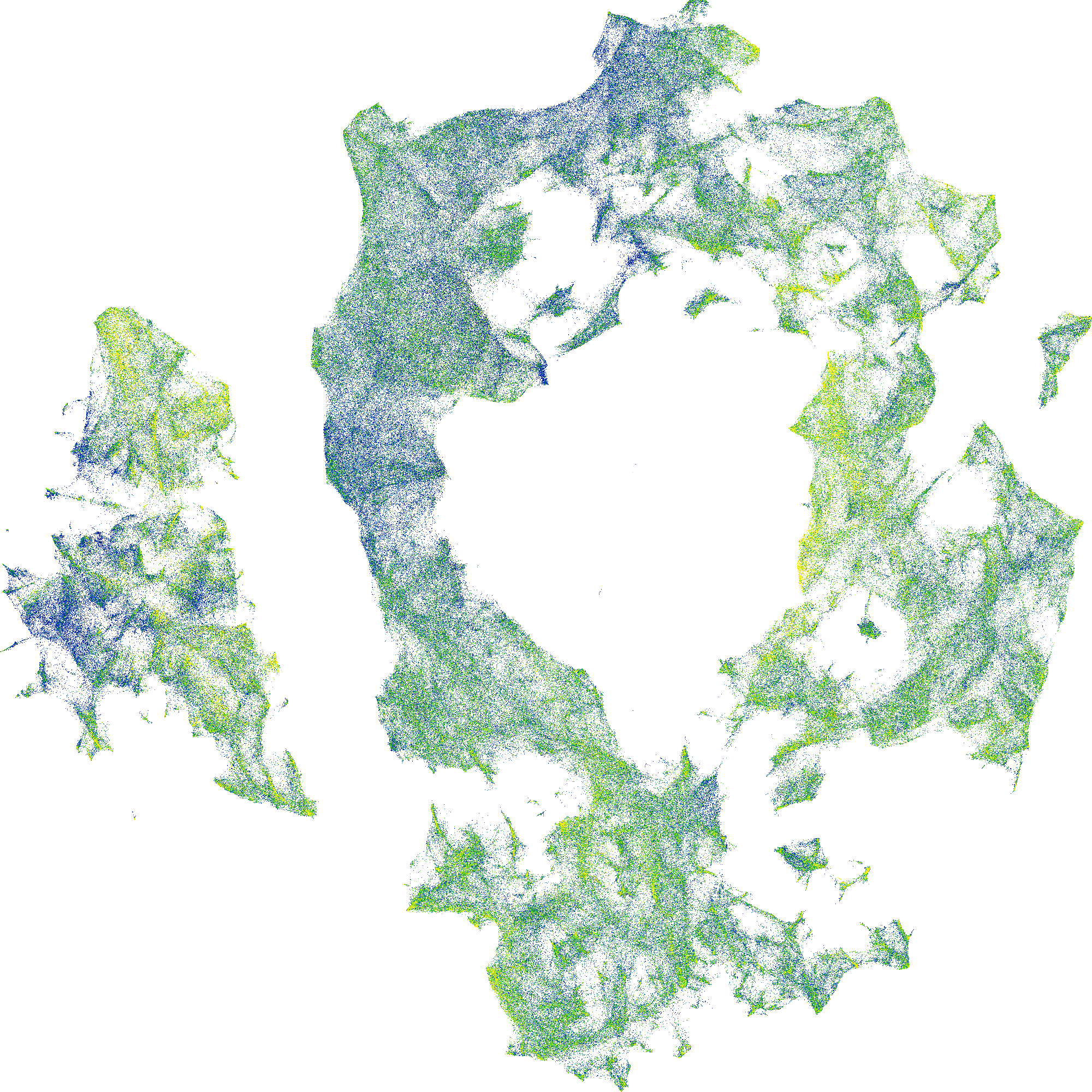
Figure 1. HUGE can learn representations on extremely large graphs (billions of nodes) at Google. (Shown here: t-SNE projection of HUGE-TPU’s Papers100M embeddings)

Graph embeddings are a common first step in graph understanding pipelines where every node in the graph is embedded(Chen et al., 2018a) into a common low-dimensional space. These embeddings are then used for graph learning tasks such as node classification, graph clustering, and link prediction (Chen et al., 2018a; Chami et al., 2022) that can be solved with standard machine learning algorithms applied in the graph embedding space without having to develop specific algorithms to directly exploit the graph structure. For example, approximate nearest neighbor search systems (Guo et al., 2020) can serve product recommendations using embeddings of user-item graphs.

Numerous methods, which we briefly review in Section 2.1, have been proposed in the literature. One of the most popular methods, DeepWalk (Perozzi et al., 2014), proposes to embed nodes via a shallow neural network trained to discriminate samples generated from random walks from random negatives. Unfortunately, the process is memory-bound, as it requires random accesses for both random walk generation and updating the embedding table. At first glance, it does not scale beyond graphs larger than a couple of millions of nodes even in the distributed setting.

Or does it? Distributed data processing workflows (such as Flume (Chambers et al., 2010) or Apache Beam) can be used to execute sampling strategies even for graphs that are too large to represent in memory on a single machine. At the same time, specialized hardware such as Tensor Processing Units (TPUs), a custom ASIC introduced in Jouppi et al. (2017), have large amounts of high-bandwidth memory that enables high-throughput gradient updates. In this work, we present a simple, TPU-based architecture for graph embedding that exploits the computational advantages of TPUs to embed billion-scale graphs. This architecture eliminates the need to develop complex algorithms to partition or synchronize the embedding table across multiple machines.

Table 1. An overview of different approaches to scaling graph embeddings up. In this work, we demonstrate a system that works without any of the yet mentioned techniques scaled to largest graphs. Scalability is given as an approximate graph size that can be processed by best-performing algorithm&system combination in a day.

Method Family	Speedup Technique	Reference Methods	Scalability
neural	—	DeepWalk, LINE, VERSE	10M
neural	graph coarsening	HARP, MILE	10M
neural	partitioning	BigGraph, EDGES, DeLNE	1000M
factorization	—	NetMF, GraRep	10k
factorization	matrix sparsification	NetSMF, NetMFSC, STRAP, NRP	100M
factorization	implicit solvers	HOPE, AROPE	100M
factorization	spectral propagation	ProNE, LightNE	1000M
factorization	matrix sketching	FastRP, RandNE, NodeSketch, InstantEmbedding	1000M

More specifically, we propose a two-phase architecture. First random walks are generated and summarized via a distributed data processing pipeline. After sampling, graph embedding is posed as a machine learning problem in the style of DeepWalk (Perozzi et al., 2014). We propose an unsupervised method for measuring embedding space quality, comparing the embedding space result to the structure of the original graph and show that the proposed system is competitive in speed and quality compared to modern CPU-based systems while achieving HUGE scale.

Graph Embeddings at Google. Graph-based machine learning is increasingly popular at Google (Perozzi et al. (2020)). There are dozens of distinct model applications using different forms of implicit and explicit graph embedding techniques in many popular Google products. Over time, these models have evolved from single-machine in-memory algorithms (similar to those dominating in academic literature) to more scalable approaches based on distributed compute platforms. In this work we detail a relatively new and very promising extension of classic graph embedding methods that we have developed in response to the need for differentiable graph embedding methods which can operate with data at extreme scale.

2. Background

In this section, we first briefly review the related work in Section 2.1. We review DeepWalk (Perozzi et al., 2014), which we use as a base for our high-performance embedding systems, in Section 2.2. We then proceed with describing two architectures for scaling Deepwalk graph embedding using commodity (HUGE-CPU) and TPU (HUGE-TPU) hardware that allow us to scale to huge graphs in Section 2.3.

2.1. Related Work

We now proceed to review the two basic approaches to embedding large graphs. Over the past years, tremendous amount of work introduced various embedding methods as well as a myriad of techniques and hardware architectures to scale them up. We summarize the related work in terms of the embedding approach, speedup techniques, and its expected scalability in Table 1.

2.1.1. Graph Embedding Approaches

We categorize embedding methods as either neural network-based or matrix factorization-based. Regardless of the approach, each method employs, sometimes implicitly, a similarity function that relates each node to other nodes in the graph. The best-performing methods depart from just using the adjacency information in the graph to some notion of random walk-based similarity, for example, personalized PageRank (PPR) (Brin and Page, 1998). A key insight for accelerating the computation of these similarities is that they are highly localized in the graph (Andersen et al., 2006), meaning 2–3 propagation steps are enough to approximate them.

Neural embedding methods view node embeddings as parameters of a shallow neural network. Neural methods optimize these parameters with stochastic gradient descent for either adjacency (Tang et al., 2015), random walk (Perozzi et al., 2014), or personalized PageRank (Tsitsulin et al., 2018) similarity functions. This optimization is done via sampling, and the updates to the embedding table are usually very sparse. Thus, random memory access typically bounds the performance of these methods.

An alternative to gradient-based methods is to directly factorize the similarity matrix. There are deep connections between neural and matrix factorization approaches (Qiu et al., 2018; Tsitsulin et al., 2021)—essentially, for many node similarities the optimal solutions for neural and factorization-based embeddings coincide. The main challenge to matrix-based methods is maintaining sparsity of intermediate representations. For large graphs, one can not afford to increase the density of the adjacency matrix nor keep too many intermediate projections.

2.1.2. Scaling Graph Embedding Systems

There are several directions for speeding up embedding algorithms—some are tailored to particular methods while some are more general. We now briefly review the most general speedup techniques. Graph coarsening (Chen et al., 2018b; Liang et al., 2021) iteratively contracts the graph, learns the embeddings for the most compressed level, and deterministically propagates the embeddings across the contraction hierarchy. Graph partitioning methods (Lerer et al., 2019; Imran et al., 2020) distribute the computation across machines while attempting to minimize communication across machines.

Early approaches to matrix factorization (Qiu et al., 2019; Yin and Wei, 2019; Yang et al., 2020b) attempt to sparsify the random walk or PPR matrices. Unfortunately, higher-order similarity matrices are still too dense for these embeddings methods to scale to very large graphs. Leveraging specialized sparse numerical linear algebra techniques (Saad, 2003) proved to be a more fruitful approach. Implicit solvers (Ou et al., 2016; Zhang et al., 2018b) can factorize the matrix without explicitly materializing it in memory. These methods are constrained to perform linear decomposition, which is not able to successfully account for structure of graphs.

Two families of techniques that produce most scalable embedding methods are spectral propagation and matrix sketching (Woodruff et al., 2014). Spectral propagation methods (Zhang et al., 2019; Qiu et al., 2021) first compute some truncated eigendecomposition of the adjacency or the Laplacian matrix of a graph and then use these eigenvectors to simulate the diffusion of information. Matrix sketching approaches approximate the similarity matrix, either iteratively (Zhang et al., 2018a; Chen et al., 2019; Yang et al., 2019) or in a single pass (Postăvaru et al., 2020). The latter option is more scalable.

2.1.3. Hardware-based Embedding Acceleration

Compared to algorithmic advances, hardware-based acceleration has arguably received less attention. Zhu et al. (2019) proposes a hybrid system that uses CPU for sampling and GPU for training the embeddings. Since the most RAM a single GPU can offer is in the order of 100 gigabytes, one can only train embeddings of 100 million node graphs on such systems. Wei et al. (2020); Yang et al. (2020a) address this problem with partitioning to include more GPUs. This approach requires tens of GPUs for a billion-node graph, which is prohibitive compared to scalable CPU-based systems, which can embed a billion-node graph on a single high-memory machine in hours.

Efficient computation of higher-order similarity is one aspect where hardware acceleration is currently lacking. Yang et al. (2021); Wang et al. (2020) propose efficient systems for random walk generation for general hardware architectures. However, in an absence of a suitable embedding method, these systems are not useful for graph embedding.

2.2. DeepWalk

Before describing our TPU embedding system, it is necessary to review DeepWalk (Perozzi et al., 2014), which is the basic method for neural graph embedding. DeepWalk adapts word2vec (Mikolov et al., 2013), a widely successful model for embedding words, to graph data. DeepWalk generates a “corpus” of short random walks; the objective of DeepWalk is to maximize the posterior probability of observing a neighboring vertex in a random walk within some specific window size. To maximize this probability efficiently, it uses hierarchical softmax (Morin and Bengio, 2005), which constructs a Huffman tree of nodes based on their frequency of appearance, or a more computationally efficient approximation, negative sampling (Gutmann and Hyvärinen, 2010). For each node that was observed within the window size from some node, DeepWalk picks $k\ll n$ uniformly at random as contrastive negative examples.

There are several computational problems with DeepWalk’s architecture, which are to be solved if we are to scale DeepWalk to graphs with billions of nodes:

• Random walk generation for large graphs is computationally prohibitive due to random memory accesses on each random walk step.

• Random walk corpus grows in size rapidly, growing much larger in size than the original sparse graph.

• Negative sampling-based optimization is also computationally prohibitive due to random memory accesses. If batched, each gradient update is bound to update a significant part of the embedding table.

To overcome the difficulties with random walk sampling, we present a distributed random walk algorithm in section 3.2 that is routinely used at Google to scale random walk simulations to web-scale graphs.

2.3. Tensor Processing Units

We proceed with briefly reviewing TPU architecture highlighting the aspects critical for our graph embedding system. A detailed review can be found in (Jouppi et al., 2017, 2021, 2023). TPUs are dedicated co-processors optimized for matrix and vector operations computed at half precision. TPUs are organized in pods, which can connect a total of 4096 of TPU chips with 32 GiB memory each, which together makes up to 128 TiB of distributed memory available for use. TPUs chips inside a pod are connected with dedicated high-speed, low-latency interconnects organized in a 3D torus topology.

2.4. Common ML Distribution Strategies

Various methods for distributing Machine Learning workloads have been discussed in the literature (Alqahtani and Demirbas, 2019) and most Machine Learning (ML) frameworks provide consistent APIs implementing multiple distribution schemes through a consistent interface. This section highlights some common distribution paradigms focusing on the techniques used to scale DeepWalk using commodity hardware (which we refer to as HUGE-CPU) and TPUs (HUGE-TPU).

TensorFlow provides the tf.distribute.Strategy abstractions to enable users to separate model creation from the training runtime environment with minimal code changes. Two common strategies are the Parameter-Server (PS) strategy and Multi-Worker Mirrored Strategy.

2.4.1. Parameter-Server Strategy

In the context of graph embedding, using a PS strategy is useful for representing a large embedding table. The PS strategy defines two compute pools of potentially heterogeneous hardware that the user can access. One pool contains machines labeled ”parameter servers” and the other pool’s machines are named ”workers”. A model’s trainable variables are sharded across the machines in the parameter-server pool which serve requests, potentially over a network, both for the values of these variables and to update them. For graph embedding, machines in the worker pool asynchronously receive batches of examples, fetch the necessary embedding rows from parameter servers over a network, compute gradients and push updates back to parameter server machines.

2.4.2. Multi-Worker Mirrored Strategy

The Multi-Worker Mirrored Strategy replicates all variables in the model on each device in a user defined pool of worker machines. A (potentially) large batch of input examples is divided among the multiple workers and proceed to compute gradients using their smaller per-replica batches. At the completion of a single step, gradients across the replicas are aggregated and all variable copies are updated synchronously. While this can accelerate computationally heavy workloads, compared to the parameter server architecture, this design has limited use in the context of Graph Embedding. Replicating embedding tables across multiple machines introduces unwanted redundancy and memory consumption.

2.4.3. TPUStrategy and Accelerated TPU Embedding Tables

Training a model (or graph embedding) in TensorFlow using TPU hardware, the TPUStrategy is very similar to the MultiWorkerMirroredStrategy. A user defines a desired TPU topology, a slice of a POD that can be thought of as a subset of interconnected processing units. Under the TPUStrategy, trainable variables are copied to all TPU replicas and large batches of examples are divided into smaller per-replica batches and distributed to available replicas and gradients are aggregated before a syncronous update. Normally, this distribution paradigm would limit the scalability of models that define large embedding tables. However, TPUs are capable of sharding embedding layers over all devices in an allocated topology and leverage high bandwidth interconnections between replicas to support accelerated sparse look-ups and gradient updates. Accelerated embedding tables are exposed in TensorFlow using the tf.tpu.experimental.embedding.TPUEmbedding (TPUEmbedding) layer and are the primary mechanism for scaling DeepWalk training on TPUs.

3. Method

We scale the DeepWalk algorithm to embed extremely large-scale graphs using two methods. The first, called HUGE-CPU, uses only commodity hardware whereas the second, HUGE-TPU, leverages modern TPUs for increased bandwidth and performance gains. Figure 2 visualizes the parameter-server architecture of HUGE-CPU. The details of parameter-server architecture are covered in section 3.3.1. Figure 3 illustrates the TPU system design behind HUGE-TPU and is detailed in section 3.3.2.

3.1. Preprocessing

One key observation is that most positional graph embedding systems cannot generate useful embeddings for nodes with less than two edges. Specifically, nodes with no edges are generally not well defined by embedding algorithms, and similarly, positional embeddings of nodes with only one edge are totally determined by the embedding of their single neighbor. Therefore, we typically prune the input graph, eliminating nodes with degree less than two. In our experiments, we only prune once though the pruning operation itself may introduce nodes that fall below the degree threshold.

3.2. Sampling

After preprocessing the graph, we run random walk sampling to generate co-occurrence tuples that will be used as the input to the graph embedding system.

A high-level overview of the distributed random walk sampling is provided in Algorithm 1. The input to the sampling component is the preprocessed graph and the output are TensorFlow Examples containing co-occurrence tuples extracted from the random walks. The implementation of the distributed random walk sampling algorithm is implemented using the distributed programming platform FlumeC++ (Chambers et al., 2010).

In the initialization phase, the distributed sampler takes as input the $\mathcal{N}$ nodes of the graph and replicates them $\gamma$ times each to create the seeds of $\gamma|\mathcal{N}|$ walks it will generate (Line 1). Next, the random sampling process proceeds in an iterative fashion, performing $k$ joins which successively grow the length of each random walk (Lines 2-4). Each join combines the walk with the node at its end point. After joining the end of the walk with its corresponding node from the graph $G$, sampling of the next node occurs (Line 4). We note that many kinds of sampling can be used here to select the next node at this step – including uniform sampling, random walks with backtracking, and other forms of weighted sampling. For the results in this paper, we consider the case of using uniform sampling. A final GroupBy operation is used to collapse the random walks down to co-occurrence counts between pairs of nodes as a function of visitation distance (Line 7).

The output of the sampling pre-processing step is a sharded series of files encoding a triple: (source_id, destination_id, co_counts). source_id is the node ID of a starting point in the random walk, the destination_id is a node ID that was arrived at during the $\gamma$ random walks and co_counts is a histogram of length walk_length containing the number of times the source_id encountered
destination_id (indexed by the random walk distance of the co-occurrence).

The DeepWalk model defines a graph reconstruction loss that has a “positive” and “negative” component. The “positive” examples are random walk paths that exist in the original graph. “Negative” examples are paths that do not exist in the original graph. If desired, the sampling step can be used to generate different varieties of negative samples (through an additional distributed sampling algorithm focusing on edges which do not exist). However, in practice, we frequently prefer to perform approximate random negative sampling “on-the-fly” while training.

Algorithm 1 Distributed Random Walk Sampling

0.  A graph $G=(V,E)$, a set of nodes to sample from $\mathcal{N}$, $\gamma$, the number of walks from each node, and $k$ the number of random walks to sample per node.

0.  $\mathcal{C}$, the co-occurrence counts between pairs of nodes in $G$ observed in the walk.

0.   // Initialize $k$ walks with each seed

1.  $walks\leftarrow\mathcal{N}.\text{repeat}(\gamma)$

2.  for step = $1...k$ do

2.      // Join each walk with the node at its end

3.     $(walks,V)\leftarrow$ $walks$.Join($G$)

3.      // Extend walk/node pair with new node

4.     $walks\leftarrow(walks,V)$.Sample()

5.  end for

5.   // Group walks from the same seeds together

6.  $node\_walks\leftarrow walks$.GroupByKey()

6.   // Aggregate co-occurrences for each node’s walks

7.  return  $\mathcal{C}\leftarrow node\_walks$.CombineValues()

3.3. Distributed training

3.3.1. HUGE-CPU

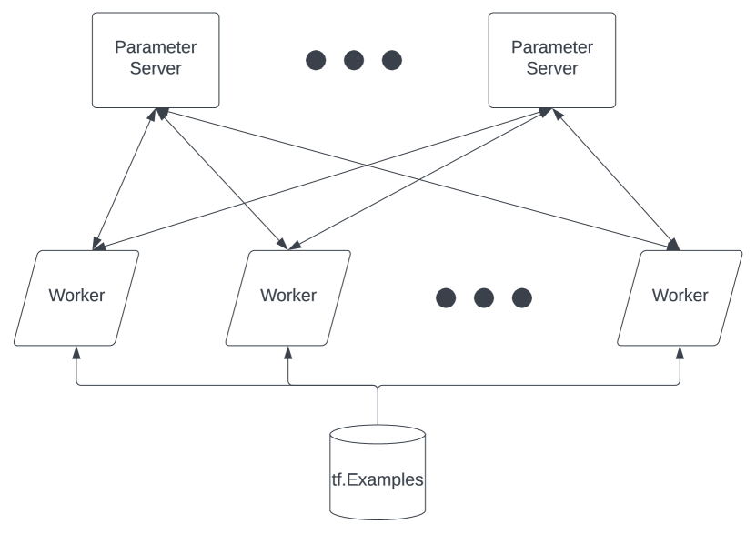
Figure 2. System diagram for the Parameter-Server (CPU) based DeepWalk model (HUGE-CPU). Two pools of machines are defined, parameter-servers and workers. Workers asynchronously fetch batches of training examples from disk and collect relevant embedding activations from parameters servers that serve requests for the sharded embedding table. Gradients are computed and updated asynchronously.

Figure 2 outlines the system design for the HUGE-CPU baseline system architecture. This system leverages distributed training with commodity hardware. Two pools of machines are defined as described in 2.4.1, a cluster of parameter-servers and a pool of workers. During initialization, trainable variables such as the large embedding table are sharded across the machines in the parameter-server pool. Workers distribute and consume batches of training examples from the output of the graph sampling pre-processing step, asynchronously fetch embedding activations from parameter servers, compute a forward pass and gradients and asynchronously push gradient updates to the relevant activations back to the parameter servers. There is no locking or imposed order of activation look-ups or updates. This enables maximum throughput of the system but comes at the cost of potentially conflicting gradient updates.

3.3.2. HUGE-TPU

Figure 3 visualizes the system design of distributed training of the DeepWalk embedding model using TPUs after the sampling procedure is complete. The replication strategy used for TPUs in conjunction with their high FLOPS per second requires generating extremely large batches of training examples for every step. The bottleneck in this system is rarely the embedding lookup or model tuning but the input pipeline to generate the large batch size required at every step.

File shards of the sampling data are distributed over the workers in a cluster dedicated to generating input data. The workers independently deserialize the co-occurrence input data and augment the source_id and destination_id pairs with negative samples, replicating source_id and randomly sampling additional destination_id node IDs uniformly from the embedding vocabulary.

The input cluster then streams the resulting training Tensors to the TPU system which de-duplicates and gathers the relevant embedding activations for the batch and distributes the computational work of computing the forward pass and gradient to the TPU replicas which are then aggregated and used to update the embedding table.

Figure 3. System diagram for accelerated HUGE unsupervised graph embedding. A large embedding table is efficiently sharded over the TPU HBM using TensorFlow TPUEmbedding layer. A cluster of machines that read, parse and randomly sample the input data is leveraged to avoid an input bottleneck. This diagram is illustrative and does not represent the true connectivity of the TPU topology.

4. Experiments

4.1. Experimental Details

Table 2. Parameters used for all HUGE-TPU and HUGE-CPU experiments. LWSGD is Stochastic Gradient Descent with a Linear Warmpup and decay learning rate schedule. The schedule is parameterized by four numbers, the number of warmup steps, the final value after warmup, the number of decay steps and the final value after the decay phase at which point the learning rate is held constant.

Parameter	HUGE-TPU	HUGE-CPU
num_walks_per_node	128	128
walk_length	3	3
Per-Replica Batch Size	4096	1024
num_neg_per_pos	31	3
Global Batch Size	$2^{24}$	$2^{19}$
LWSGD	(5K, 0.01, 100K, 0.001)	N/A
SGD	N/A	0.001

4.1.1. Datasets

For testing the scalability of our methods, we resort to random graphs. We resort to the standard (degree-free) Stochastic Block Model (Nowicki and Snijders, 2001), which is a generative graph model that divides $n$ vertices into $k$ classes, and then places edges between two vertices $v_{i}$ and $v_{j}$ with probability $p_{ij}$ determined from the class assignments. Specifically, each vertex $v_{i}$ is given a class $y_{i}\in\{1,\ldots,k\}$, and an edge $\{v_{i},v_{j}\}$ is added to the edge set $E$ with probability $P_{y_{i}y_{j}}$, where $P$ is a symmetric $k\times k$ matrix containing the between/within-community edge probabilities. Assortative clustering structure in a graph can be induced using the SBM by setting the on-diagonal probabilities of $P$ higher than the off-diagonal probabilities. For benchmarking, we set $P_{y_{i}y_{j}}=q$ iff $i=j$ and to $p$ otherwise.

Complementing our analysis on synthetic benchmark datasets, we also study the performance of the methods on two large real-world graphs: Friendster (Yang and Leskovec, 2012) and OGBN-Papers100m (Hu et al., 2020). We report the dataset statistics in Table 3.

4.1.2. Baselines

First we compare HUGE-CPU and HUGE-TPU with other state-of-the-art scalable graph embedding algorithms: InstantEmbedding (Postăvaru et al., 2020), PyTorch-BigGraph (Lerer et al., 2019) and LightNE (Qiu et al., 2021) on an end-to-end node classification task using the OGBN-Papers100m dataset. We further explore the embedding space quality of each algorithm using both the OGBN-Papers100m and Friendster datasets. Finally we compare embedding space quality metrics as a function of training time to explore the speedups of HUGE-TPU compared to HUGE-CPU using a randomly generated graphs with 100M (SBM-100M) and 1B nodes SBM-1000M.

Table 3. Datasets we use for our experimental studies. We report the total number of nodes and edges in all graphs.

Name	$\lvert{}V\rvert$	$\lvert{}E\rvert$
Friendster	65.6M	3612M
OGB-Papers100M	111M	1616M
SBM-10M	10M	100M
SBM-100M	100M	1000M
SBM-1000M	1000M	10000M

4.2. Parameters for HUGE methods

Table 2 shows the parameters used by the HUGE-CPU and HUGE-TPU methods. The random walk sampling procedure describe in 3.2 was executed sampling $\gamma=128$ walks per node with a walk length of $k=3$. The set of samples were shared for all experiments involving HUGE-CPU and HUGE-TPU to minimize the affect of random sampling on the results. num_neg_per_pos is the number of random negative destinations sampled for every ”positive” example drawn from the sampling pre-processing step. The global batch size for HUGE-TPU may be computed as $\texttt{per\_replica\_batch\_size}*(1+\texttt{num\_neg\_per\_pos})$. A step is not well defined for the HUGE-CPU algorithm since workers asynchronously pull variables and push updates. Due to the increased computational power and high bandwidth interconnections between replicas, HUGE-TPU achieves a much higher throughput and global per-step batch size. Training with extremely large batch sizes can be challenging. We have found that a Stochastic Gradient Descent (SGD) optimizer with a linear warmup and ramp down gives good results. HUGE-CPU was also trained with a SGD optimizer but uses a fixed learning rate.

4.3. Evaluation Metrics

For all other graphs besides OGBN-Papers100m, there are no ground-truth labels for node classification. This problem is not unique to publicly available large graphs—in our practical experience, oftentimes there is need to evaluate and compare different embedding models in an unsupervised fashion. We propose simple unsupervised metrics to compare the embedding quality of different embeddings of a graph. For the analysis, we $L_{2}$-normalize all embeddings.

We also report four self-directed metrics for evaluation we use in our production system to monitor the embedding quality. First, edge signal-to-noise ratio (edge SNR) defined as:

$$\mathrm{SNR}=\frac{\mathbb{E}_{u,v\not\in{}E}\left[d(u,v)\right]}{\mathbb{E}_{u,v\in{}E}\left[d(u,v)\right]},$$

where we approximate the numerator term by taking a random sub-sample of all non-edges. In our experiments, we also show the entire distribution of edge- and non-edge distances. The intuition behind these metrics is that the distance between nodes that are connected in the original graph (a “true” edge) should be “closer” than nodes that are not adjacent in the input graph. Last, we compute the sampled version of the edge recall (Tsitsulin et al., 2018). We sample 100 nodes, pick $k$ closest nodes in the embedding space forming a set $S$. Then, sampled recall is:

$$\mathrm{recall}@k(u)=\frac{|{}N(u)\cap{}S|}{k}.$$

Despite small sample size, the recall is stable and, coupled with the edge SNR, it is a useful indicator of the reconstruction performance of different graph embedding methods.

Figure 4. Unsupervised embedding analysis results for OGBN-Papers100m. We see that HUGE-TPU has superior edge SNR compared to all baselines.

Figure 5. Embedding analysis results for Friendster. HUGE-TPU achieves the best edge SNR due to better distance distributions.

Figure 6. Embedding analysis results for SBM-100M. This figure compares training HUGE-CPU for 3, 12 and 36 billion training examples compared to the results of HUGE-TPU and InstantEmbedding.

Figure 7. Embedding analysis results for SBM-1000M to explore the embedding space quality as a function of training time for HUGE-CPU compared to HUGE-TPU and InstantEmbedding.

4.4. Downstream Embedding Quality

Being the fastest embedding system is not enough – we also want embedding vectors to be as useful as possible. Every percentage point of quality on downstream tasks directly translates to missed monetary opportunities. Therefore, in our experience, when working on scalable versions of algorithms, it is critical to maintain high embedding quality.

Table 4. Embedding quality as measured by downstream task accuracy, relative speed, and hardware used for four different embedding methods. Speed normalized to the runtime of HUGE-CPU.

Method	Quality	Speedup	Hardware
PyTorch-BigGraph	43.64	23.0	16x A100 GPUs
LightNE	27.90	40.8	160 vCPUs
InstantEmbedding	53.15	3.5	64 vCPUs
HUGE-CPU	56.03	1	5120 vCPUs
HUGE-TPU	56.13	9.9	4x4x4 v4 TPUs

To that end, we provide one of the first studies of embedding scalability and performance across different hardware architectures. We compare with the fastest single-machine CPU embedding available (Qiu et al., 2021) and industrial-grade GPU embedding system (Lerer et al., 2019). Note that these systems have a much more restrictive limit for a maximum number of nodes that they can process. PyTorch-BigGraph can not process graphs with more than $1.4\times{}10^{9}$ nodes on the current hardware, assuming a system with the latest-generation GPUs and highest available memory. LightNE does not have such restriction, but it keeps both the graph and the embedding table in memory. Because of that, scalability into multi-billion node embedding territory is still an open question for that system.

Table 4 presents the embedding quality results on the OGB-Papers100M dataset. For measuring the embedding quality, we follow the Open Graph Benchmark evaluation protocol (Hu et al., 2020) with a simple logistic regression model. We skip tuning the model parameters on the validation set, and report the accuracy of predictions on the test set. We also report the relative speedup over the CPU DeepWalk embedding implementation. HUGE-TPU is the only one that maintains the end-to-end classification quality provided by DeepWalk and improves runtime efficiency relative HUGE-CPU by an order of magnitude.

4.5. Self-directed Embedding Space Evaluation

To better understand the differences in downstream model performance, we present our self-directed metric for datasets with no ground-truth labels. We analyze the embedding space quality with the proposed metrics comparing HUGE-CPU, HUGE-TPU, InstantEmbedding, PyTorch-BigGraph and LightNE. To that end, we report the results on 2 real and 2 synthetic datasets, presented in Figures 4-5 and 6-7, respectively.

Interestingly, the results are fairly consistent across all datasets considered. We see that HUGE-TPU provides superior separation between the distributions of edges and non-edges, achieving a very high edge signal to noise ratio. We also see that the sampled edge recall metric on is generally much harder to optimize for on very large graphs, and that HUGE-TPU meets or exceeds the performance of its comparable baseline HUGE-CPU.

4.6. Visualization

In order to better understand our embeddings, we frequently resort to visualizations. Figure 8 shows a plot of the entire embedding space of OGBN-Papers100M dataset for HUGE-TPU and LightNE, projected via t-SNE (Van der Maaten and Hinton, 2008). Compared to HUGE-TPU, the LightNE embedding demonstrated surprisingly poor global clustering structure, which explains its subpar downstream task performance we covered in Section 4.4.

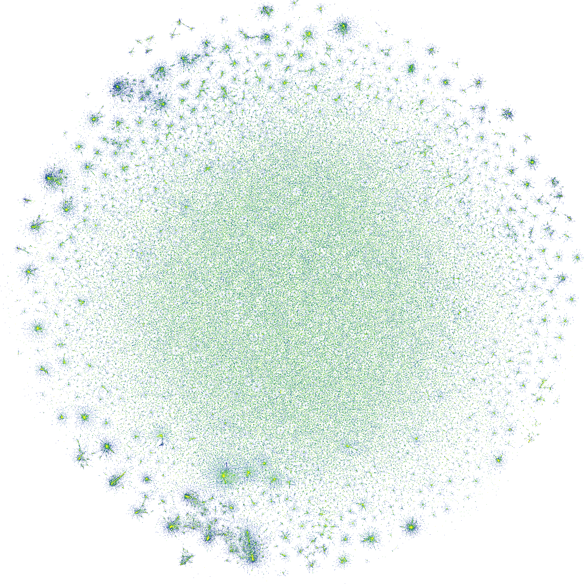
Figure 8. Visualization of the entire embedding space of (left) HUGE-TPU and (right) LightNE embeddings of the Papers100M dataset, projected via t-SNE with the same parameters. Colors indicate point density. We can observe much better clustered structure in HUGE-TPU embeddings which directly translates to significantly better downstream prediction quality.

4.7. Discussion

Table 5. The average examples per seconds processed by HUGE-CPU and HUGE-TPU for all reported experiments. HUGE-CPU used 128 Parameter Servers and 128 Workers with 20 cores each. HUGE-TPU was configured with a v4 in a 64 chip configuration. We report the total number of examples processed per second relative to HUGE-CPU

Method	Relative Examples Per Second
HUGE-CPU	1
HUGE-TPU	173x

While both HUGE-CPU and HUGE-TPU can horizontally scale according to the user configuration, we use the same topologies throughout all experiments. HUGE-CPU uses 128 Parameter Server machines and 128 Workers with 20 cores each and 2GiB of RAM. HUGE-TPU uses a v4 TPU with 64 replicas. The total training examples processed by HUGE-TPU relative to HUGE-CPU for this configuration is shown in table 5. Since the throughput of HUGE-CPU and HUGE-TPU is fixed for a given topology and batch size, the throughput is constant thought all experiments.

As shown in table 4, HUGE-TPU achieves the highest accuracy in the end-to-end node classification task using the OGBN-Papers100m dataset though HUGE-CPU not far behind. However, while HUGE-CPU is able to scale horizontally to handle extremely large embedding spaces, in-memory and hardware accelerated achieve orders of magnitude speedups compared to HUGE-CPU.

When analyzing the embedding space quality metrics however, in terms of HUGE-TPU consistently achieves superior performance. The distribution of distances between adjacent nodes for HUGE-TPU is typically much smaller than the other methods as is reflected by an SNR that is consitently orders of magnitude larger than other methods. The consistently high SNR is probably due to the extremely high throughput compared with HUGE-CPU.

To further explore the affect of throughput on the system, we ran HUGE-CPU for multiple fixed number of training steps: 3B, 12B and 36B, while fixing the TPU training time on the SBM-100M and SBM-1000M datasets. In relative terms, HUGE-CPU-3B took approximately half the time of HUGE-TPU, HUGE-CPU-12B was trained for 2x the time of HUGE-TPU and HUGE-CPU-36B was trained for 6x the allowed time of HUGE-TPU. We also compare these results with InstantEmbedding to contrast the Deepwalk style embeddings with a matrix factorization graph embedding method. Predictably, the results show that the HUGE-CPU will ”converge” or at least approach, over time, the performance of InstantEmbedding in terms of edge/non-edge distributions and recall. However, HUGE-TPU consistently outperforms both InstantEmbedding and HUGE-CPU in terms of SNR and edge and non-edge distance distributions even when HUGE-CPU is allowed to train for more than 6x more time than HUGE-TPU.

To summarize, we comprehensively demonstrate the quality and performance of HUGE-TPU over HUGE-CPU as well as state-of-the-art industrial-grade systems for graph embeddings. First, we showed that on a largest-scale labelled embedding data, HUGE-TPU achieves state-of-the-art performance while being order of magnitude faster than comparable CPU-based system. We then proceed with unsupervised embedding evaluations we use in deployed production systems at Google. We show how HUGE-TPU is competitive in embedding quality over both real and synthetic tasks, only improving its performance compared to the baselines as the size of the graphs increases.

5. Conclusion

In this work we have examined the problem of scalable graph embedding from a new angle: TPU systems with large amounts of shared low-latency high-throughput memory. We build a system (HUGE) that does not suffer from key performance issues of the previous work, and greatly simplifies the system design. HUGE is deployed at Google, in a variety of different graph embedding applications. Our experiments demonstrate the merits of using accelerators for graph embedding. They show that the HUGE-TPU embedding is competitive in speed with other scalable approaches while delivering embeddings which are more performant. In fact, the embeddings learned with HUGE-TPU are of the same quality as running the full embedding algorithm (with no compromises for its speed).

Appendix A Experiment setup

The following setups were used for the experiments with PyTorch-BigGraph and LightNE.

PyTorch-BigGraph.

• Google Cloud machine: a2-megagpu-16g, 96 vCPUs, 1.33 TB memory. 16x NVIDIA A100 40GB.

• Image: Debian 10 based Deep Learning VM for PyTorch CPU/GPU with CUDA 11.3 M98

• BigGraph version as of September 2022 (git@2e94f8a).

• Configuration Friendster:

  ⬇

  dimension=128, comparator="cos", num_epochs=2, batch_size=100000, num_batch_negs=1000, num_uniform_negs=1000, eval_fraction=0.01, num_gpus=16

• Configuration Papers100m:

  ⬇

  dimension=128, comparator="cos", num_epochs=3, batch_size=100000, num_batch_negs=1000, num_uniform_negs=1000, eval_fraction=0.01, num_gpus=16

LightNE

• Google Cloud machine: m1-ultramem-160, 160 vCPUs, 3.84 TB memory.

• Image: Debian 11, v20220920

• LightNE version: version as of September 2022 (git@c43afc4)

• Configuration:

  ⬇

  -walksperedge 10000 -walklen 3 -step_coeff 1,1,1 -rounds 1 -s -m -ne_method netsmf -rank 256 -dim 128 -order 10 -sample_ratio 17 -mem_ratio 0.5 -negative 1 --sparse_project 0 -sample 1 -upper 0 -analyze 1

References

- (1)
- Alqahtani and Demirbas (2019) Salem Alqahtani and Murat Demirbas. 2019. Performance Analysis and Comparison of Distributed Machine Learning Systems. https://doi.org/10.48550/ARXIV.1909.02061
- Andersen et al. (2006) Reid Andersen, Fan Chung, and Kevin Lang. 2006. Local graph partitioning using pagerank vectors. In FOCS. IEEE, 475–486.
- Brin and Page (1998) Sergey Brin and Lawrence Page. 1998. The anatomy of a large-scale hypertextual web search engine. Computer networks and ISDN systems 30, 1-7 (1998), 107–117.
- Chambers et al. (2010) Craig Chambers, Ashish Raniwala, Frances Perry, Stephen Adams, Robert Henry, Robert Bradshaw, and Nathan. 2010. FlumeJava: Easy, Efficient Data-Parallel Pipelines. In ACM SIGPLAN Conference on Programming Language Design and Implementation (PLDI).
- Chami et al. (2022) Ines Chami, Sami Abu-El-Haija, Bryan Perozzi, Christopher Ré, and Kevin Murphy. 2022. Machine learning on graphs: A model and comprehensive taxonomy. JMLR (2022).
- Chen et al. (2018a) Haochen Chen, Bryan Perozzi, Rami Al-Rfou, and Steven Skiena. 2018a. A tutorial on network embeddings. arXiv preprint arXiv:1808.02590 (2018).
- Chen et al. (2018b) Haochen Chen, Bryan Perozzi, Yifan Hu, and Steven Skiena. 2018b. HARP: Hierarchical representation learning for networks. In AAAI.
- Chen et al. (2019) Haochen Chen, Syed Fahad Sultan, Yingtao Tian, Muhao Chen, and Steven Skiena. 2019. Fast and accurate network embeddings via very sparse random projection. In CIKM. 399–408.
- Guo et al. (2020) Ruiqi Guo, Philip Sun, Erik Lindgren, Quan Geng, David Simcha, Felix Chern, and Sanjiv Kumar. 2020. Accelerating Large-Scale Inference with Anisotropic Vector Quantization. In ICML.
- Gutmann and Hyvärinen (2010) Michael Gutmann and Aapo Hyvärinen. 2010. Noise-contrastive estimation: A new estimation principle for unnormalized statistical models. In AISTATS. JMLR Workshop and Conference Proceedings, 297–304.
- Hu et al. (2020) Weihua Hu, Matthias Fey, Marinka Zitnik, Yuxiao Dong, Hongyu Ren, Bowen Liu, Michele Catasta, and Jure Leskovec. 2020. Open graph benchmark: Datasets for machine learning on graphs. NeurIPS (2020).
- Imran et al. (2020) Mubashir Imran, Hongzhi Yin, Tong Chen, Yingxia Shao, Xiangliang Zhang, and Xiaofang Zhou. 2020. Decentralized embedding framework for large-scale networks. In International Conference on Database Systems for Advanced Applications. Springer, 425–441.
- Jouppi et al. (2021) Norman P. Jouppi, Doe Hyun Yoon, Matthew Ashcraft, Mark Gottscho, Thomas B. Jablin, George Kurian, James Laudon, Sheng Li, Peter Ma, Xiaoyu Ma, Thomas Norrie, Nishant Patil, Sushma Prasad, Cliff Young, Zongwei Zhou, and David Patterson. 2021. Ten Lessons From Three Generations Shaped Google’s TPUv4i : Industrial Product. In 2021 ACM/IEEE 48th Annual International Symposium on Computer Architecture (ISCA). 1–14. https://doi.org/10.1109/ISCA52012.2021.00010
- Jouppi et al. (2023) Norman P. Jouppi, George Kurian, Sheng Li, Peter Ma, Rahul Nagarajan, Lifeng Nai, Nishant Patil, Suvinay Subramanian, Andy Swing, Brian Towles, Cliff Young, Xiang Zhou, Zongwei Zhou, and David Patterson. 2023. TPU v4: An Optically Reconfigurable Supercomputer for Machine Learning with Hardware Support for Embeddings. arXiv:2304.01433 [cs.AR]
- Jouppi et al. (2017) Norman P. Jouppi, Cliff Young, Nishant Patil, David Patterson, Gaurav Agrawal, Raminder Bajwa, Sarah Bates, Suresh Bhatia, Nan Boden, Al Borchers, Rick Boyle, Pierre luc Cantin, Clifford Chao, Chris Clark, Jeremy Coriell, Mike Daley, Matt Dau, Jeffrey Dean, Ben Gelb, Tara Vazir Ghaemmaghami, Rajendra Gottipati, William Gulland, Robert Hagmann, C. Richard Ho, Doug Hogberg, John Hu, Robert Hundt, Dan Hurt, Julian Ibarz, Aaron Jaffey, Alek Jaworski, Alexander Kaplan, Harshit Khaitan, Andy Koch, Naveen Kumar, Steve Lacy, James Laudon, James Law, Diemthu Le, Chris Leary, Zhuyuan Liu, Kyle Lucke, Alan Lundin, Gordon MacKean, Adriana Maggiore, Maire Mahony, Kieran Miller, Rahul Nagarajan, Ravi Narayanaswami, Ray Ni, Kathy Nix, Thomas Norrie, Mark Omernick, Narayana Penukonda, Andy Phelps, and Jonathan Ross. 2017. In-Datacenter Performance Analysis of a Tensor Processing Unit. https://arxiv.org/abs/1704.04760
- Lerer et al. (2019) Adam Lerer, Ledell Wu, Jiajun Shen, Timothee Lacroix, Luca Wehrstedt, Abhijit Bose, and Alex Peysakhovich. 2019. PyTorch-BigGraph: A Large-scale Graph Embedding System. In SysML.
- Liang et al. (2021) Jiongqian Liang, Saket Gurukar, and Srinivasan Parthasarathy. 2021. MILE: A multi-level framework for scalable graph embedding. In AAAI. 361–372.
- Mikolov et al. (2013) Tomas Mikolov, Ilya Sutskever, Kai Chen, Greg S Corrado, and Jeff Dean. 2013. Distributed representations of words and phrases and their compositionality. NIPS (2013).
- Morin and Bengio (2005) Frederic Morin and Yoshua Bengio. 2005. Hierarchical probabilistic neural network language model. In AISTATS. PMLR, 246–252.
- Nowicki and Snijders (2001) Krzysztof Nowicki and Tom A B Snijders. 2001. Estimation and prediction for stochastic blockstructures. Journal of the American statistical association (2001).
- Ou et al. (2016) Mingdong Ou, Peng Cui, Jian Pei, Ziwei Zhang, and Wenwu Zhu. 2016. Asymmetric transitivity preserving graph embedding. In KDD. 1105–1114.
- Perozzi et al. (2014) Bryan Perozzi, Rami Al-Rfou, and Steven Skiena. 2014. DeepWalk: Online learning of social representations. In KDD. 701–710.
- Perozzi et al. (2020) Bryan Perozzi, Jakub Łącki, and Vahab Mirrokni. 2020. Graph Mining and Learning at Google. NeurIPS Workshop (2020). https://gm-neurips-2020.github.io/
- Postăvaru et al. (2020) Ştefan Postăvaru, Anton Tsitsulin, Filipe Miguel Gonçalves de Almeida, Yingtao Tian, Silvio Lattanzi, and Bryan Perozzi. 2020. InstantEmbedding: Efficient local node representations. arXiv preprint arXiv:2010.06992 (2020).
- Qiu et al. (2021) Jiezhong Qiu, Laxman Dhulipala, Jie Tang, Richard Peng, and Chi Wang. 2021. LightNE: A lightweight graph processing system for network embedding. In SIGMOD. 2281–2289.
- Qiu et al. (2019) Jiezhong Qiu, Yuxiao Dong, Hao Ma, Jian Li, Chi Wang, Kuansan Wang, and Jie Tang. 2019. NetSMF: Large-scale network embedding as sparse matrix factorization. In The World Wide Web Conference. 1509–1520.
- Qiu et al. (2018) Jiezhong Qiu, Yuxiao Dong, Hao Ma, Jian Li, Kuansan Wang, and Jie Tang. 2018. Network embedding as matrix factorization: Unifying DeepWalk, LINE, PTE, and node2vec. In WSDM. 459–467.
- Saad (2003) Yousef Saad. 2003. Iterative methods for sparse linear systems. SIAM.
- Tang et al. (2015) Jian Tang, Meng Qu, Mingzhe Wang, Ming Zhang, Jun Yan, and Qiaozhu Mei. 2015. LINE: Large-scale information network embedding. In WWW. 1067–1077.
- Tsitsulin et al. (2018) Anton Tsitsulin, Davide Mottin, Panagiotis Karras, and Emmanuel Müller. 2018. VERSE: Versatile graph embeddings from similarity measures. In WWW. 539–548.
- Tsitsulin et al. (2021) Anton Tsitsulin, Marina Munkhoeva, Davide Mottin, Panagiotis Karras, Ivan Oseledets, and Emmanuel Müller. 2021. FREDE: anytime graph embeddings. VLDB (2021), 1102–1110.
- Van der Maaten and Hinton (2008) Laurens Van der Maaten and Geoffrey Hinton. 2008. Visualizing data using t-SNE. Journal of machine learning research 9, 11 (2008).
- Wang et al. (2020) Rui Wang, Yongkun Li, Hong Xie, Yinlong Xu, and John CS Lui. 2020. GraphWalker: An I/O-Efficient and Resource-Friendly Graph Analytic System for Fast and Scalable Random Walks. In USENIX. 559–571.
- Wei et al. (2020) Wanjing Wei, Yangzihao Wang, Pin Gao, Shijie Sun, and Donghai Yu. 2020. A distributed multi-GPU system for large-scale node embedding at Tencent. arXiv preprint arXiv:2005.13789 (2020).
- Woodruff et al. (2014) David P Woodruff et al. 2014. Sketching as a tool for numerical linear algebra. Foundations and Trends® in Theoretical Computer Science 10, 1–2 (2014), 1–157.
- Yang et al. (2020a) Dongxu Yang, Junhong Liu, and Junjie Lai. 2020a. EDGES: An efficient distributed graph embedding system on GPU clusters. IEEE Transactions on Parallel and Distributed Systems 32, 7 (2020), 1892–1902.
- Yang et al. (2019) Dingqi Yang, Paolo Rosso, Bin Li, and Philippe Cudre-Mauroux. 2019. NodeSketch: Highly-efficient graph embeddings via recursive sketching. In KDD. 1162–1172.
- Yang and Leskovec (2012) Jaewon Yang and Jure Leskovec. 2012. Defining and evaluating network communities based on ground-truth. In Proceedings of the ACM SIGKDD Workshop on Mining Data Semantics. 1–8.
- Yang et al. (2021) Ke Yang, Xiaosong Ma, Saravanan Thirumuruganathan, Kang Chen, and Yongwei Wu. 2021. Random Walks on Huge Graphs at Cache Efficiency. In Proceedings of the ACM SIGOPS 28th Symposium on Operating Systems Principles. 311–326.
- Yang et al. (2020b) Renchi Yang, Jieming Shi, Xiaokui Xiao, Yin Yang, and Sourav S Bhowmick. 2020b. Homogeneous network embedding for massive graphs via reweighted personalized pagerank. VLDB (2020).
- Yin and Wei (2019) Yuan Yin and Zhewei Wei. 2019. Scalable graph embeddings via sparse transpose proximities. In KDD. 1429–1437.
- Zhang et al. (2019) Jie Zhang, Yuxiao Dong, Yan Wang, Jie Tang, and Ming Ding. 2019. ProNE: Fast and Scalable Network Representation Learning.. In IJCAI. 4278–4284.
- Zhang et al. (2018a) Ziwei Zhang, Peng Cui, Haoyang Li, Xiao Wang, and Wenwu Zhu. 2018a. Billion-scale network embedding with iterative random projection. In ICDM. IEEE.
- Zhang et al. (2018b) Ziwei Zhang, Peng Cui, Xiao Wang, Jian Pei, Xuanrong Yao, and Wenwu Zhu. 2018b. Arbitrary-order proximity preserved network embedding. In KDD.
- Zhu et al. (2019) Zhaocheng Zhu, Shizhen Xu, Jian Tang, and Meng Qu. 2019. GraphVite: A high-performance cpu-gpu hybrid system for node embedding. In The World Wide Web Conference. 2494–2504.