SuperInpaint: Learning Detail-Enhanced Attentional Implicit Representation for Super-resolutional Image Inpainting

Abstract

In this work, we introduce a challenging image restoration task, referred to as SuperInpaint, which aims to reconstruct missing regions in low-resolution images and generate completed images with arbitrarily higher resolutions. We have found that this task cannot be effectively addressed by stacking state-of-the-art super-resolution and image inpainting methods as they amplify each other’s flaws, leading to noticeable artifacts. To overcome these limitations, we propose the detail-enhanced attentional implicit representation (DEAR) that can achieve SuperInpaint with a single model, resulting in high-quality completed images with arbitrary resolutions. Specifically, we use a deep convolutional network to extract the latent embedding of an input image and then enhance the high-frequency components of the latent embedding via an adaptive high-pass filter. This leads to detail-enhanced semantic embedding. We further feed the semantic embedding into an unmask-attentional module that suppresses embeddings from ineffective masked pixels. Additionally, we extract a pixel-wise importance map that indicates which pixels should be used for image reconstruction. Given the coordinates of a pixel we want to reconstruct, we first collect its neighboring pixels in the input image and extract their detail-enhanced semantic embeddings, unmask-attentional semantic embeddings, importance values, and spatial distances to the desired pixel. Then, we feed all the above terms into an implicit representation and generate the color of the specified pixel. To evaluate our method, we extend three existing datasets for this new task and build 18 meaningful baselines using SOTA inpainting and super-resolution methods. Extensive experimental results demonstrate that our method outperforms all existing methods by a significant margin on four widely used metrics.

1 Introduction

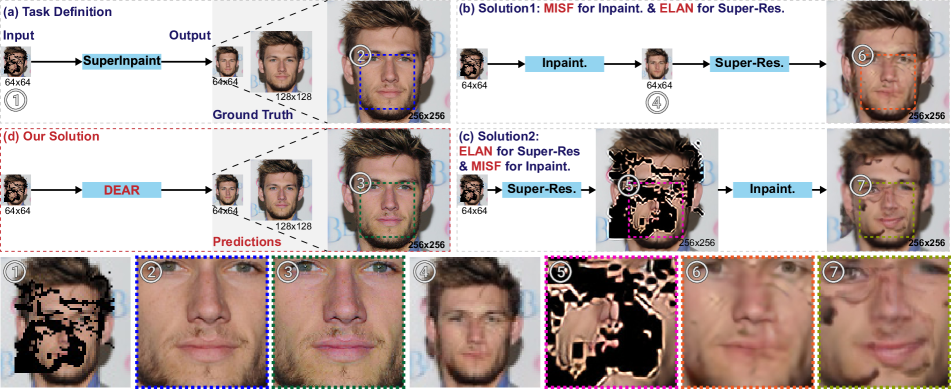
Figure 1: Visualization of SuperInpaint task (i.e.,(a)), two baseline solutions (i.e., (b) & (c)), and our solution (i.e., (d) DEAR). For the two naive solutions, we use the state-of-the-art image inpainting method (i.e., MISF [17]) and image super-resolution method (i.e., ELAN [47]). We enlarge seven regions or images at the last row for better visualization.

Image inpainting methods [30, 10, 21, 8, 22, 25] have been widely used in recent years and achieved promising results, but they still face practical limitations. Many damaged images are often old and low in resolution. To obtain the best possible view, people often need to complete missing pixels while upscaling these images to higher resolutions. The naive choice is to combine the current inpainting and super-resolution (SR) methods directly. However, the performance of such a solution will drop significantly since these two tasks are not directly relevant to each other. Current SR methods add new pixels based on their nearby features, which can have a negative impact on the entire image when the mask area (i.e., large missing regions) is involved (See Fig. 1 (c)). Additionally, if the inpainting method generates some flaws, even if they are invisible to the human eye, the SR model can further worsen the results (See Fig. 1 (b)).

To overcome these limitations, we focus on a challenging task called SuperInpaint that aims to reconstruct missing regions in the input image and generate high-fidelity and completed images with arbitrarily higher resolutions (See Fig. 1 (a)). SuperInpaint has great potential in image inpainting, super-resolution, and old photo restoration areas but cannot be properly addressed by stacking state-of-the-art inpainting and super-resolution methods (See solutions in Fig. 1 (b) and (c)). In this paper, we propose to realize SuperInpaint via the implicit image representation [5]. However, SuperInpaint has some specific challenges that cannot be properly addressed by the previous work [5, 15]: First, the arbitrary high-resolution generation requires that the details in the input image should be involved and enhanced in the representation. Second, the effects of the masked pixels on the semantic embedding should be considered. Third, ineffective masked pixels (i.e., unrecoverable masked pixels) should be excluded during the reconstruction process.

To address these challenges, we propose the detail-enhanced attentional implicit representation (DEAR) with three key modules, i.e., the detail-enhanced semantic embedding (DSE) extraction, unmask-attentional semantic embedding (USE) extraction, and importance map extraction. We first extract the latent embedding of an input image and then use DSE to enhance its high-frequency components. After that, the embedding is further passed to USE to suppress the information from ineffective masked pixels. Moreover, we extract a pixel-wise importance map to indicate which pixels should be used for image reconstruction. During the testing process, given the coordinates of a pixel we want to reconstruct, we first obtain the pixel’s neighboring pixels within the input image and extract the DSE, USE, and importance values of all neighboring pixels as well as their spatial distances to the desired pixel. Then, we feed all the above extractions to the implicit representation (i.e., multi-layer perceptrons (MLPs)) and get the reconstruction result. As shown in Fig. 1 (d), the proposed method can generate high-fidelity images at different resolutions with rich details. Overall, the main contributions are as follows:

• We identify a challenging task, i.e., SuperInpaint that is to reconstruct missing regions in a low-resolution image and generate high-fidelity and completed images with arbitrarily higher resolutions.

• We build 18 baseline methods based on SOTA inpainting and SR methods for this new task and study their effectiveness and limitations.

• We propose a novel approach for this task, which is denoted as detail-enhanced attentional implicit representation (DEAR) with novel designed modules.

• We construct new corrupted image datasets in different resolutions based on previous datasets CelebAHQ [23], Places365 [51], and FFHQ [13] by adding masks on the low-resolution counterparts. We conduct extensive experiments on these datasets, which demonstrates the advantages of our method over all existing methods.

2 Related Work

Image Inpainting. Image inpainting [45, 41, 34, 43, 31, 11, 33, 52, 19, 29] aims to restore damaged images by filling in the missing regions according to the non-missing portions. Several existing approaches [30, 28, 18] leverage prior information to get realistic results, e.g., [28, 30] use edge information and smoothed images to guide the restoration respectively. [18] performs semantic segmentation and image completion simultaneously to ensure the clear object boundaries. In contrast, [21] employs a novel partial convolution technique that only uses valid pixels to infer the missing pixels. [10] uses an element-wise convolution block to reconstruct missing regions around the mask boundary and a generative network to handle other missing regions. [17] improves upon [10] by performing element-wise filtering at both the feature and image levels, where the feature-level filtering focuses on large missing regions and image-level filtering handles local details. However, traditional image inpainting methods cannot change the image resolution, thus they cannot be deployed on  SuperInpaint task directly.

Image Super-resolution. The goal of SR task [50, 9, 42, 7, 44, 38, 14, 26, 40] is to increase the image resolution. Non-learning based methods like Bilinear interpolation add new pixels according to nearby pixels. Thanks to the development of neural network, early regression-based methods such as RCAN [48], RRDB [35], and EDSR [20] can restore the image by learning from the high-level feature and global information. Then GAN-based methods [3] are proposed based on its generation capacity. However, those model can only upscale images in certain ratios. To overcome this limitation, Liif [5] builds a reflection between pixel feature and RGB colour using implicit neural representation, which reconstructs image in arbitrary resolutions. However, traditional SR models are incapable to deal with the corrupted input in our setting.

Implicit Neural Representation. Implicit neural representations can parameterize a continuous differentiable signal with a neural network, which have been widely used in 2D and 3D tasks [37, 24, 16, 36, 39, 49, 2]. Nerf [27] uses implicit neural field to generate the novel view from differen perspectives. IM-NET [6] uses implicit neural function to store the value of point cloud points for 3D shape representation. LTE [15] modifies LIIF by adding more high-frequency information in Fourier space, solving the drawback that a standalone MLP is biased toward learning low-frequency knowledge. And NERV [4] uses an MLP to store video frames, which is suitable for video compression. Similar as previous works, we choose a implicit neural representation to build the relationship between pixel information and RGB color.

3 SuperInpaint and Motivation

3.1 Problem Formulation

Given a masked low-resolution image $\mathbf{I}^{\text{LR}}\in\mathds{R}^{H\times W\times 3}$ where some regions are missing (See Fig. 1), the task SuperInpaint aims to reconstruct the missing pixels in $\mathbf{I}^{\text{LR}}$ and generate arbitrary higher resolution images denoted as $\mathbf{I}^{\text{HR}}\in\mathds{R}^{sH\times sW\times 3}$, the variable $s>1.0$ denotes the magnification fraction. The missing regions are indicated by a binary mask tensor $\mathbf{M}\in\mathds{R}^{H\times W}$.

Intuitively, this task could be naively addressed by stacking two existing tasks, e.g., super-resolution (SR) and image inpainting. Specifically, we can first use a SR method to handle $\mathbf{I}^{\text{LR}}$ and get a high-resolution image with missing regions. Then, we can further conduct the image inpainting on the high-resolution image to complete the missing pixels. Similarly, we can also change the execution order and perform image inpainting and super-resolution sequentially. To show the challenges of SuperInpaint and limitations of the above naive solutions, we select a SOTA image inpainting method (i.e., MISF [17]) and a SOTA SR method (i.e., ELAN [47]). Those two methods can consist of two baselines for the SuperInpaint: MISF→ELAN and ELAN → MISF. We analyze their limitations in the following.

3.2 Naive Solutions and Limitations

We take the CelebAHQ dataset [23] as an example to construct a dataset for SuperInpaint. We have the training and testing datasets (i.e., $\mathcal{D}_{\text{train}}$ and $\mathcal{D}_{\text{test}}$) of CelebAHQ with a high resolution (i.e., $256\times 256$). Then, we resize them to low-resolution images (i.e., $64\times 64$) and get datasets $\mathcal{D}_{\text{train}}^{\text{LR}}$ and $\mathcal{D}_{\text{test}}^{\text{LR}}$. After that, we mask each image of $\mathcal{D}_{\text{train}}$, $\mathcal{D}_{\text{train}}$, $\mathcal{D}_{\text{train}}^{\text{LR}}$ and $\mathcal{D}_{\text{test}}^{\text{LR}}$ via mask maps from a third-part mask set [21], and get the corresponding datasets $\mathcal{C}_{\text{train}}$, $\mathcal{C}_{\text{test}}$, $\mathcal{C}_{\text{train}}^{\text{LR}}$, and $\mathcal{C}_{\text{test}}^{\text{LR}}$. We can apply two baselines, i.e., MISF→ELAN and ELAN → MISF, on the constructed dataset.

• MISF→ELAN: We first train MISF with low-resolution images $\mathcal{D}_{\text{train}}^{\text{LR}}$ and the corresponding masked images $\mathcal{C}_{\text{train}}^{\text{LR}}$. MISF is fed with a masked low-resolution image and outputs a completed low-resolution image. Then, we train ELAN with low-resolution dataset $\mathcal{D}_{\text{train}}^{\text{LR}}$ and the corresponding high-resolution dataset $\mathcal{D}_{\text{train}}$. We follow default setups in the released codes of MISF and ELAN. During the testing process, we feed an image from $\mathcal{C}_{\text{test}}^{\text{LR}}$ to MISF and ELAN sequentially and get a completed higher-resolution image.

• ELAN → MISF: Similar with MISF→ELAN, we first train ELAN with $\mathcal{D}_{\text{train}}^{\text{LR}}$ and $\mathcal{D}_{\text{train}}$. Then, we train MISF with high-resolution images $\mathcal{D}_{\text{train}}$ and the corresponding masked images $\mathcal{C}_{\text{train}}$. During the testing process, we feed an image from $\mathcal{C}_{\text{test}}^{\text{LR}}$ to ELAN and MISF sequentially and get a completed higher-resolution image.

We visualize an example of MISF→ELAN and ELAN → MISF in Fig. 1 and see that: ❶ MISF→ELAN (i.e., Fig. 1 (b)) can complete the missing pixels with x4 higher resolution. Nevertheless, there are a lot of artifacts around the filled regions of the output (See Fig. 1 (b)). This is because the super-resolution method is trained to handle normal pixels and cannot properly address the restored pixels, leading to magnified artifacts. ❷ ELAN→MISF cannot restore natural, enlarged, and completed images. As shown in Fig. 1 (c), a lot of black regions remain in the final output. The main reason lies in: First, the SOTA super-resolution method (i.e., ELAN [47]) cannot properly handle the pixels around mask boundaries since it does not see these examples during the training process, leading to distorted and enlarged mask boundaries (See Fig. 1). Second, the distorted mask boundaries are further fed to the inpainting method (i.e., MISF[17]) which also does not see such examples during training, leading to undesired artifacts.

Overall, naively stacking existing inpainting and super-resolution methods cannot address the SuperInpaint task since they cannot handle the special patterns (e.g., completed low-resolution pixels or distorted mask boundaries) of intermediate stages. We could retrain the inpainting and super-resolution models to overcome new situations. However, this leads to huge extra training costs and the retraining of one model should be adapted to another one. A novel end-to-end approach is urgently required.

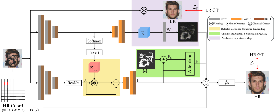
Figure 2: The overall structure of detail-enhanced attentional implicit representation (DEAR). It is mainly composed of detailed-enhanced semantic embedding extraction, unmask-attentional semantic embedding extraction, and pixel-wise importance map extraction.

4 Methodology - DEAR

4.1 Overview

Instead of the two-stage solutions in Sec. 3, we propose an end-to-end one-stage method to achieve the SuperInpaint task, i.e., detail-enhanced attentional implicit representation (DEAR), which is able to complete missing regions while restoring images in arbitrary resolution. The intuitive idea is to reconstruct a pixel’s color conditional on another pixel based on its detail-enhanced semantic embedding, unmask-attentional embedding, importance, and spatial distance between the two pixels. Specifically, given a pixel $\mathbf{p}=(x_{p},y_{p})$ in the input $\mathbf{I}^{\text{LR}}\in\mathds{R}^{H\times W\times 3}$, we want to reconstruct the color (i.e., $c_{q}$) of another pixel at the coordinate $\mathbf{q}=(x_{q},y_{q})$ that could be continuous coordinated by

$$c_{q}(\mathbf{p})=\phi_{\theta}(\mathbf{F}_{\mathbf{p}},\mathbf{E}_{\mathbf{p}},\mathbf{W}_{\mathbf{p}},\chi(\mathbf{p},\mathbf{q})),$$ (1)

where $\mathbf{F}_{\mathbf{p}}$ denotes the detail-enhanced semantic embedding of the $\mathbf{p}$th pixel, $\mathbf{E}_{\mathbf{p}}$ is the unmask-attentional embedding of the $\mathbf{p}$th pixel, $\mathbf{W}_{\mathbf{p}}$ indicates the importance of $\mathbf{p}$th pixel for reconstructing the pixel $\mathbf{q}$, and the function $\chi(\mathbf{p},\mathbf{q})$ calculates the spatial distance between the two pixels. The output $c_{q}(\mathbf{p})$ represents the color of $\mathbf{q}$th pixel conditional on the $\mathbf{p}$th pixel, and the function $\phi_{\theta}(\cdot)$ is the desired implicit representation with parameters $\theta$. Note that, once we have a trained Eq. (1), we can calculate the color of arbitrary coordinates.

Intuitively, we can regard all pixels in $\mathbf{I}^{\text{LR}}$ as the pixel $\mathbf{p}$ to reconstruct the pixel $\mathbf{q}$. Here, we select spatially neighboring pixels and get the $\mathbf{q}$’s color by

$$c_{q}=\sum_{\mathbf{p}\in\mathcal{N}_{q}}w_{p}c_{q}(\mathbf{p}),$$ (2)

where $\mathcal{N}_{q}$ denotes the set of neighboring pixels around $\mathbf{q}$, and the weight $w_{p}$ is determined by spatial distance between $\mathbf{p}$ and $\mathbf{q}$ and normalized to make sure $\sum_{\mathbf{p}\in\mathcal{N}_{q}}w_{p}=1$.

The rationales behind the above design are as follows: ❶ Previous works [15, 1] show that deep models like CNNs are usually biased towards learning low-frequency features. However, details (i.e., high-frequency parts) are critical to generate high-fidelity images. Hence, we aim to enhance the detailed information (e.g., high-frequency information) in the semantic embedding and get $\mathbf{F}_{\mathbf{p}}$ (See Sec. 4.2). ❷ The unmasked pixels in the input image are the only reliable information for image restoration. The generative embeddings of masked pixels may affect the implicit representation. As detailed in Sec. 4.3, we propose to highlight the embeddings of unmasked regions while suppressing the ones of masked pixels. ❸ If the pixel $\mathbf{p}$ is around the masked regions and can not be recovered accurately, it should not be used to reconstruct the pixel $\mathbf{q}$ in Eq. (1). Hence, we need a weight $\mathbf{W}_{\mathbf{p}}$ to indicate whether a pixel should be used or not, which is illustrated in Sec. 4.4. We will validate the effectiveness of all modules in the experimental section.

4.2 Detailed-enhanced Semantic Embedding

We propose to enhance the high-frequency parts of the semantic embedding for the implicit representation. Given an encoder $\varphi_{\beta}(\cdot)$, we extract the latent embedding of the input image $\mathbf{I}$ and get $\mathbf{Z}\in\mathds{R}^{H_{z}\times W_{z}\times C_{z}}$ by $\varphi_{\beta}(\mathbf{I})$. Then, we aim to extract the high-frequency components of the $\mathbf{Z}$. A straightforward solution is to use high-pass filters to handle each channel of the $\mathbf{Z}$ and add the filtering results back to the input, that is, we have

$$\hat{\mathbf{Z}}=\mathbf{Z}+\mathbf{K}_{\text{hp}}\circledast\mathbf{Z},$$ (3)

where $\mathbf{K}_{\text{hp}}\in\mathds{R}^{H_{z}\times W_{z}\times C_{z}K_{z}^{2}}$ contains the element-wise high-pass filters for each channel. The operation ‘$\circledast$’ denotes element-wise filtering. The key challenge is how to make the high-pass filters adapt to different inputs and spatial variations. Inspired by [17, 53], we predict high-pass filters w.r.t. different inputs

$$\mathbf{K}_{\text{hp}}=\mathbf{1}-\text{softmax}(\varphi_{\hat{\beta}}(\mathbf{I})),$$ (4)

where $\varphi_{\hat{\beta}}(\cdot)$ has a similar architecture with $\varphi_{\beta}(\cdot)$ but with independent parameters and is to predict low-pass filters. Then, we subtract the low-pass filters from the all-one tensor and get high-pass filters. Note that, we add a softmax layer to the end of $\varphi_{\hat{\beta}}(\cdot)$ to make sure the predicted kernels are low-pass, which makes the predicted kernel weights positive and the summation along channel dimension be one.

After getting the detailed-enhanced latent embedding (i.e., $\hat{\mathbf{Z}}$), we further feed it to a decoder (i.e., $\varphi^{-1}_{\beta^{-1}}(\cdot)$) to get a detailed-enhanced embedding $\mathbf{F}\in\mathds{R}^{H\times W\times C}$ with the same resolution as the input

$$\mathbf{F}=\varphi^{-1}_{\beta^{-1}}(\hat{\mathbf{Z}}),$$ (5)

where $\mathbf{F}_{\mathbf{p}}$ in Eq. (1) is the $\mathbf{p}$th element of $\mathbf{F}$.

4.3 Unmask-attentional Semantic Embedding

We aim to suppress embeddings of ineffective masked pixels. Intuitively, the embeddings of some masked pixels could be recovered by the generative encoder and decoder network (e.g., $\varphi_{\beta}(\cdot)$ and $\varphi^{-1}_{\beta^{-1}}(\cdot)$) while some masked pixels cannot. We denote the unrecoverable pixels as the ineffective masked pixels whose embeddings should be suppressed. To this end, we first obtain all unmasked embeddings via the mask $\mathbf{M}$ and $\mathbf{F}$ in Eq. (5) and have

$$\mathbf{F}_{\text{M}}=(1-\mathbf{M})\odot\mathbf{F},$$ (6)

where ‘$\odot$’ is the element-wise multiplication. Then, we use the attention operation to calculate weights to measure the ineffective embeddings

$$\mathbf{E}=\text{softmax}(\frac{\mathbf{F}_{\text{M}}\otimes\mathbf{F}^{\text{T}}}{\sqrt{\text{d}_{\text{K}}}})\otimes\mathbf{F},$$ (7)

where ‘$\otimes$’ is the matrix production, ’$\text{d}_{\text{K}}$’ is the feature channel, and ’T’ means matrix transpose. $\mathbf{E}$ reflects the effectiveness of each pixel.

4.4 Pixel-wise Importance Map

We also add a new branch to generate the importance of each pixel, i.e., $\mathbf{W}$. Specifically, we add two convolution layers (See Fig. 2) to map the latent feature $\varphi_{\hat{\beta}}(\mathbf{I})$ to pixel-wise kernels $\mathbf{K}\in\mathds{R}^{H\times W\times K^{2}}$ and use these kernels to reconstruct the pixels in the input image. For the $\mathbf{p}$th pixel in the input, we can know its $K\times K$ neighboring pixels denoted as the set $\mathcal{N}_{p}$ and reconstruct the $\mathbf{p}$th pixel by linearly combining the neighboring pixels via the predicted kernels

$$\hat{\mathbf{I}}[\mathbf{p}]=\sum_{\mathbf{q}\in\mathcal{N}_{p}}\mathbf{K}_{\mathbf{p}}[\mathbf{p}-\mathbf{q}]\cdot\mathbf{I}[\mathbf{q}],$$ (8)

where $\hat{\mathbf{I}}[\mathbf{p}]$ denotes the reconstructed pixel. Our intuitive idea is that if a pixel could be properly reconstructed via its neighboring pixels, this pixel could be used in the implicit representation and the corresponding importance score $\mathbf{W}_{\mathbf{p}}$ should be high and towards one. The predicted kernel can represent the capability of the linear reconstruction and we can generate the importance map by

$$\mathbf{W}=\text{Conv}(\mathbf{K}).$$ (9)

We also visualize the pixel-level importance map in Fig. 2. The pixels in the large masked area will be assigned lower importance scores. On the contrary, the pixels in unmasked regions and small corrupted regions are given higher importance stores, since small regions can be restored much more easily. Those results show that proposed importance map can reflect whether certain pixels should be considered during the reconstruction.

4.5 Implementation Details

Network architecture. As shown in Fig. 2, our encoder $\varphi_{\beta}(\cdot)$ contains three convolution layers and eight ResNet blocks. For convolution layers, the kernel sizes are 7, 4, and 4. The strides are set to 2. The decoder $\varphi^{-1}_{\beta^{-1}}$ is composed of two transposed convolution layers, whose kernel sizes are 4 and strides are 2. This feature extractor makes sure the generated feature F has the same resolution as the input. Our implicit neural function $\phi_{\theta}$ is parameterized by a four-layer MLP with 256 latent dimensions.

Loss functions. We choose the L1 loss during the training step. The predicted pixel color $c_{q}$ and ground truth pixel color are used to calculate the HR level reconstruction loss $\mathcal{L}_{1}$. And as illustrated in Sec. 4.4, pixel-wise kernel can be applied on corrupted input to get the reconstructed LR image, which is used to calculate the LR level reconstruction loss $\mathcal{L}_{2}$. The final object function is

$$\mathcal{L}=\mathcal{L}_{1}+0.01*\mathcal{L}_{2}.$$ (10)

Hyperparameters. When training all models, we use Adam as the optimizer ($\beta_{1}$= 0.9, $\beta_{2}$ = 0.999), the learning rate is 0.0001 and it delays by half every 100 epochs. All models are trained for 200 epochs on two NVIDIA Tesla V100 GPUs and the batch size is set to 16.

5 Experimental Results

5.1 Setups

	Metric	MISF→				BI	EDSR	LTE	ELAN	LAMA→				BI	EDSR	LTE	ELAN	LTE	DEAR
		BI	EDSR	LTE	ELAN	→MISF				BI	EDSR	LTE	ELAN	→LAMA
CelebAHQ	PSNR $\uparrow$	25.55	26.83	26.09	26.89	26.28	22.83	22.65	21.06	25.70	26.36	25.48	26.41	25.03	22.59	22.17	22.63	28.26	29.84
	SSIM$\uparrow$	0.871	0.872	0.829	0.873	0.878	0.840	0.781	0.766	0.831	0.857	0.840	0.856	0.818	0.829	0.758	0.814	0.855	0.968
	L1 $\downarrow$	0.037	0.053	0.041	0.031	0.057	0.081	0.070	0.086	0.034	0.030	0.042	0.031	0.090	0.184	0.423	0.106	0.025	0.022
	LPIPS $\downarrow$	0.331	0.143	0.070	0.141	0.413	0.704	0.070	0.273	0.214	0.175	0.204	0.175	0.325	0.414	0.518	0.328	0.236	0.053
Places365	PSNR $\uparrow$	20.81	21.49	21.29	22.08	19.47	17.97	19.04	18.47	21.56	21.55	21.93	22.43	18.82	17.88	18.27	18.36	23.87	25.61
	SSIM$\uparrow$	0.626	0.645	0.704	0.635	0.546	0.630	0.587	0.600	0.682	0.702	0.622	0.758	0.569	0.527	0.587	0.581	0.722	0.824
	L1 $\downarrow$	0.068	0.090	0.065	0.094	0.074	0.070	0.064	0.313	0.059	0.056	0.054	0.049	0.093	0.178	0.273	0.091	0.041	0.040
	LPIPS $\downarrow$	0.307	0.205	0.250	0.311	0.609	0.487	0.370	0.545	0.341	0.347	0.475	0.287	0.430	0.522	0.514	0.380	0.354	0.170
FFHQ	PSNR $\uparrow$	24.48	25.13	24.95	25.26	22.10	19.60	19.29	20.28	24.19	24.86	23.16	24.84	22.30	20.32	20.35	20.84	27.93	28.97
	SSIM$\uparrow$	0.842	0.861	0.777	0.866	0.821	0.749	0.712	0.786	0.821	0.847	0.828	0.844	0.824	0.709	0.751	0.752	0.851	0.879
	L1 $\downarrow$	0.037	0.034	0.047	0.033	0.108	0.252	0.250	0.320	0.037	0.033	0.044	0.034	0.088	0.195	0.416	0.100	0.026	0.023
	LPIPS $\downarrow$	0.200	0.168	0.359	0.164	0.462	0.573	0.569	0.448	0.232	0.191	0.323	0.196	0.334	0.429	0.542	0.303	0.246	0.160

Table 1: Results from DEAR and proposed baselines on CelebAHQ [12], Places365 [51], and FFHQ datasets [13]. The baselines are generated using previous inpainting models (MISF [17] and LAMA [32]), and SR models (Bilinear Interpolation(BI), EDSR [20], LTE [15], and ELAN [47]).

Method	Upscale Ratio
	$\times$1.5	$\times$2	$\times$3.5	$\times$4	$\times$5.5	$\times$6	$\times$7.5	$\times$8
MISF→BI	29.53/0.970	27.46/0.935	26.11/0.905	25.55/0.871	25.56/0.811	24.65/0.799	24.34/0.805	23.94/0.758
MISF→EDSR	–	27.30/0.921	–	26.83/0.872	–	25.39/0.817	–	25.43/0.799
MISF→LTE	27.41/0.892	26.40/0.848	26.11/0.805	26.09/0.829	25.71/0.768	25.38/0.766	24.58/0.760	24.35/0.758
MISF→ELAN	–	26.71/0.909	–	26.89/0.873	–	25.77/0.825	–	24.79/0.785
BI→MISF	27.04/0.949	27.02/0.937	26.42/0.892	26.28/0.878	25.90/0.844	25.64/0.832	24.83/0.805	24.32/0.794
EDSR→MISF	–	24.62/0.910	–	22.83/0.840	–	22.97/0.805	–	22.47/0.773
LTE→MISF	22.92/0.866	22.90/0.849	22.85/0.800	22.65/0.781	21.78/0.725	21.65/0.714	21.43/0.692	21.34/0.686
ELAN→MISF	–	24.23/0.897	–	21.06/0.766	–	20.54/0.717	–	19.93/0.680
LTE	26.05/0.865	29.08/0.906	28.19/0.854	28.82/0.872	28.21/0.824	28.37/0.817	27.76/0.804	27.70/0.799
DEAR	33.11/0.986	31.32/0.977	30.07/0.971	29.84/0.968	29.13/0.932	29.13/0.924	28.93/0.887	28.19/0.859

Table 2: Results from the DEAR and baselines on CelebAHQ [12] dataset under different upscale ratios. We use PSNR/SSIM to evaluate the performance.

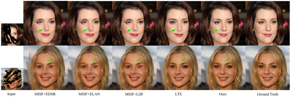
Figure 3: Qualitative results on CelebAHQ [12] dataset.

Datasets. Since SuperInpaint is the new proposed task, no previous dataset can be used directly in our setting. We modify three widely used datasets CelebAHQ [12], Places365 [51], and FFHQ [13]. CelebAHQ is a large-scale face image dataset that contains 30,000 high-resolution face images selected from the CelebA dataset [23]. Places365 is a huge scene dataset that contains 1.8 million images from 365 scene categories. FFHQ is composed of 70,000 high-quality human images which are variable in terms of age, ethnicity, and background. To get the corrupted LR image, we down-sample the HR image and add the mask from the irregular mask dataset [21].

Baselines. We combine the inpainting models (MISF [17] and LAMA [32]) and SR models (Bilinear Interpolation(BI), EDSR [20], LTE [15], and ELAN [47]) to generate baselines as discussed in Sec. 3.2. The inpainting models are trained for LR and HR images separately to fit different input sizes. We also test the performance of LTE on SuperInpaint task directly.

Evaluation metrics. We choose four widely used image quality metrics PSNR (peak signal-to-noise ratio), SSIM (structural similarity index), L1, and LPIPS [46] (perceptual similarity) to evaluate the performance of all networks. PSNR, SSIM, and L1 reflect the quality of the generated image. LPIPS measures the perceptual distance between the restored image and ground truth.

5.2 Quantitative Results

We show the results from DEAR and baselines on CelebAHQ, Places365, and FFHQ datasets in Table 1. Proposed method earns the best PSNR, SSIM, L1, and LPIPS scores compared with all baselines. On CelebAHQ dataset, compared with MISF→LTE, our model DEAR gets 3.75 higher PSNR and improves the SSIM by 13.9%. Compared with LTE, DEAR can improve the PSNR by 1.58 and increase the SSIM by 11.3%. On Places365 dataset, compared with LAMA→LTE, DEAR boosts the PSNR by 3.68. DEAR brings 10.2% SSIM improvement in contrast to LTE. On FFHQ dataset, our model lowers the L1 by 0.003 and LPIPS by 0.086 in contrast to LTE. Those results show that the model combination cannot address the SuperInpaint challenge. DEAR combines the merits from inpainting and SR tasks and earns promising results, since it preserves more high-frequency information and reconstructs the corrupted area with the help of the unmasked area information and importance map.

In Table 2, we show the reconstruction ability of DEAR and baselines under different upscale ratios. DEAR and LTE [15] are trained on $\times$4 setting. ELAN [47] and EDSR [20] need to be trained separately on each setting. On $\times$2 setting, DEAR improves PSNR by 4.02 and SSIM by 5.6% when compared with MISF→EDSR. On $\times$8 setting, our model brings 0.49 PSNR improvement in contrast to LTE. We can see that DEAR earns the best performance under all ratios with the help of implicit neural function and effective model components, while proposed baselines suffer from poor performance and upscale ratio restriction.

5.3 Qualitative Results

To further justify the ability of DEAR, we show qualitative results from our model and baselines. The qualitative results on CelebAHQ dataset are shown in Figure 3, and the results from Places365 dataset are shown in Figure 4. Those baselines are unable to generate reliable results because SR models will amplify the flaws in reconstructed LR image. LTE cannot restore the corrupted area correctly, since it doesn’t learn enough information from unmasked regions. Compared with those methods, our method generates more high-fidelity outputs. As illustrated in the second row of Figure 3, DEAR preserves more texture information in the hair area. As shown in the first row of Figure 4, DEAR generates more details in the stone part.

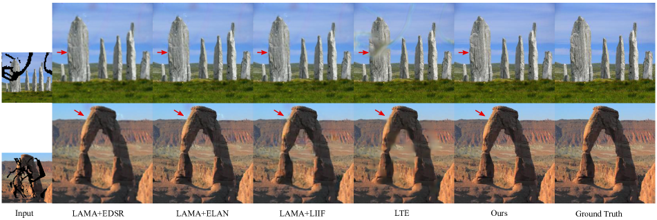
Figure 4: Qualitative results on Places365 [51] dataset.

5.4 Ablation Study

SR capability of DEAR.

DEAR can be used on the traditional SR task directly, where the input is the clean low-resolution image. To justify the SR ability of DEAR, we compare its results with LIIF [5] and LTE [15] under several upscale ratios. All models are trained under $\times$4 setting. As shown in Table 3, compared with LIIF, DEAR boosts the PSNR by 0.48 on $\times$2 setting and highlights SSIM to 82.6% on $\times$8 setting. DEAR can optimize the PSNR by 1.9 on $\times$2 setting in contrast to LTE. Proposed network uses high-pass filters to preserve more high-frequency information which plays a key role in image reconstruction.

Method	Upscale Ratio
	$\times$2	$\times$4	$\times$6	$\times$8
LIIF	34.32/0.963	30.98/0.882	30.13/0.838	29.83/0.819
LTE	32.90/0.955	31.77/ 0.897	30.93/0.841	30.15/0.821
DEAR	34.80/0.976	31.39/0.890	30.48/0.846	30.17/0.826

Table 3: Study on SR ability of DEAR on FFHQ [13] dataset. We use PSNR/SSIM to evaluate the performance.

Inpainting capability of DEAR.

DEAR can also be used on inpainting task directly, where the input and output have the same resolution. The results are shown in Table 4. On the CelebAHQ dataset, compared with MISF, DEAR raises the PSNR by 0.21. On the Places365 dataset, our model can increase the PSNR by 0.59 in contrast to MISF. Those results show that DEAR also has good inpainting ability even compared with SOTA inpainting models. The unmask-attentional semantic embedding and pixel-wise importance map guarantee that our method has a high generalization capability.

Method	CelebAHQ				Places365
	PSNR$\uparrow$	SSIM$\uparrow$	L1 $\downarrow$	LPIPS$\downarrow$	PSNR$\uparrow$	SSIM$\uparrow$	L1 $\downarrow$	LPIPS$\downarrow$
LAMA	33.36	0.990	0.011	0.012	28.26	0.962	0.025	0.047
MISF	34.28	0.991	0.012	0.011	30.09	0.969	0.022	0.041
DEAR	34.49	0.974	0.010	0.017	30.68	0.950	0.021	0.039

Table 4: Study on inpainting ability of DEAR.

Model components.

To show that all model components aid the performance improvement, we do ablation experiments by adding each DEAR part iteratively. As shown in Table 5, on CelebAHQ dataset, adding detailed-enhanced semantic embedding (DSE) can improve the PSNR by 0.95 and improve SSIM by 2.2%. Those results show the necessity of high-frequency information. Adding unmask-attentional semantic embedding (USE) can bring 0.77 PSNR improvement and lower the L1 by 0.007. The pixel-wise importance map (PIM) can help the model highlight the SSIM by 1.5% meanwhile lowering LPIPS by 0.034.

We also show the output from each model variant in Figure 5. We can see that the base model gets a poor result, leaving many blurred parts. The high frequency feature helps the model recover more detail information. The models with USE and PIM can reconstruct more realistic images.

Variant	CelebAHQ				Places365
	PSNR$\uparrow$	SSIM$\uparrow$	L1 $\downarrow$	LPIPS$\downarrow$	PSNR$\uparrow$	SSIM$\uparrow$	L1 $\downarrow$	LPIPS$\downarrow$
Base	27.21	0.916	0.035	0.121	23.93	0.755	0.046	0.239
+DSE	28.16	0.948	0.030	0.094	24.66	0.786	0.042	0.224
+USE	28.93	0.953	0.023	0.087	25.01	0.793	0.043	0.213
+PIM	29.84	0.968	0.022	0.053	25.61	0.824	0.040	0.170

Table 5: Ablation study on DEAR components by adding detailed-enhanced semantic embedding (DSE), unmask-attentional semantic embedding (USE), and pixel-wise importance map (PIM).

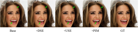
Figure 5: Outputs from DEAR variants after adding detailed-enhanced semantic embedding (DSE), unmask-attentional semantic embedding (USE), and pixel-wise importance map (PIM).

5.5 Difference to Existing Implicit Representations

In this part, we analyze the performance of LIIF [5] , LTE [15] and DEAR on SuperInpaint task. All three models can be used to restore the images in arbitrary higher resolutions. The quantitative results are shown in Table 6, and qualitative results are shown in Figure 6. LIIF uses implicit neural representation to reconstruct arbitrary resolution images firstly, but it ignores some high-frequency information due to MLP characteristics. To overcome this drawback, LTE adds high-frequency embeddings in Fourier domain. DEAR uses a high-pass filter to enhance the high-frequency feature. As shown in Table 2 and Table 3, LTE faces significant performance drop in the low-upscale ratios, while DEAR maintains high performance under all ratios. LIIF and LTE are unable to learn sufficient information from the unmasked region, leaving many blurred areas. We further propose unmask-attentional semantic embedding to suppress the undesired pixel features. We generate pixel-wise importance map to tell the model whether certain pixels should be considered or not. Those components help DEAR generate high-fidelity image in arbitrary resolutions.

Method	CelebAHQ				Places365
	PSNR$\uparrow$	SSIM$\uparrow$	L1 $\downarrow$	LPIPS$\downarrow$	PSNR$\uparrow$	SSIM$\uparrow$	L1 $\downarrow$	LPIPS$\downarrow$
LIIF	27.91	0.841	0.029	0.252	23.38	0.716	0.047	0.356
LTE	28.26	0.855	0.025	0.236	23.87	0.722	0.041	0.354
DEAR	29.84	0.968	0.022	0.053	25.61	0.824	0.040	0.170

Table 6: Comparisons among LIIF [5], LTE [15], and DEAR on SuperInpaint task.

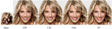
Figure 6: Outputs from LIIF [5], LTE [15], and DEAR on SuperInpaint task.

6 Conclusions

In this paper, we identified a challenging image restoration task named SuperInpaint. Given a low-resolution image with large missing regions, SuperInpaint is to fill in the missing pixels while generating high-fidelity images with arbitrarily higher resolutions. We proposed the detail-enhanced attentional implicit representation (DEAR) to achieve this task with three new designs including detail-enhanced semantic embedding extraction, unmask-attentional semantic embedding extraction, and pixel-wise importance map extraction. We also built 18 baseline methods based on state-of-the-art inpainting and super-resolution methods and constructed three new datasets for SuperInpaint based on existing public datasets. The extensive results demonstrate that DEAR outperforms all baselines significantly.

References

- [1] Salma Abdel Magid, Yulun Zhang, Donglai Wei, Won-Dong Jang, Zudi Lin, Yun Fu, and Hanspeter Pfister. Dynamic high-pass filtering and multi-spectral attention for image super-resolution. In ICCV, pages 4288–4297, 2021.
- [2] Yukang Cao, Guanying Chen, Kai Han, Wenqi Yang, and Kwan-Yee K Wong. Jiff: Jointly-aligned implicit face function for high quality single view clothed human reconstruction. In CVPR, pages 2729–2739, 2022.
- [3] Kelvin CK Chan, Xintao Wang, Xiangyu Xu, Jinwei Gu, and Chen Change Loy. Glean: Generative latent bank for large-factor image super-resolution. In CVPR, pages 14245–14254, 2021.
- [4] Hao Chen, Bo He, Hanyu Wang, Yixuan Ren, Ser Nam Lim, and Abhinav Shrivastava. Nerv: Neural representations for videos. In M. Ranzato, A. Beygelzimer, Y. Dauphin, P.S. Liang, and J. Wortman Vaughan, editors, NIPS, volume 34, pages 21557–21568. Curran Associates, Inc., 2021.
- [5] Yinbo Chen, Sifei Liu, and Xiaolong Wang. Learning continuous image representation with local implicit image function. In CVPR, pages 8628–8638, 2021.
- [6] Zhiqin Chen and Hao Zhang. Learning implicit fields for generative shape modeling. In CVPR, pages 5939–5948, 2019.
- [7] Riccardo de Lutio, Alexander Becker, Stefano D’Aronco, Stefania Russo, Jan D Wegner, and Konrad Schindler. Learning graph regularisation for guided super-resolution. In CVPR, pages 1979–1988, 2022.
- [8] Qiaole Dong, Chenjie Cao, and Yanwei Fu. Incremental transformer structure enhanced image inpainting with masking positional encoding. In CVPR, pages 11358–11368, June 2022.
- [9] Baisong Guo, Xiaoyun Zhang, Haoning Wu, Yu Wang, Ya Zhang, and Yan-Feng Wang. Lar-sr: A local autoregressive model for image super-resolution. In CVPR, pages 1909–1918, 2022.
- [10] Qing Guo, Xiaoguang Li, Felix Juefei-Xu, Hongkai Yu, Yang Liu, and Song Wang. Jpgnet: Joint predictive filtering and generative network for image inpainting. In ACM Multimedia, pages 386–394, 2021.
- [11] Xiefan Guo, Hongyu Yang, and Di Huang. Image inpainting via conditional texture and structure dual generation. In ICCV, pages 14134–14143, 2021.
- [12] Tero Karras, Timo Aila, Samuli Laine, and Jaakko Lehtinen. Progressive growing of gans for improved quality, stability, and variation. ICLR, 2018.
- [13] Tero Karras, Samuli Laine, and Timo Aila. A style-based generator architecture for generative adversarial networks. In CVPR, pages 4401–4410, 2019.
- [14] Xiangtao Kong, Xina Liu, Jinjin Gu, Yu Qiao, and Chao Dong. Reflash dropout in image super-resolution. In CVPR, pages 6002–6012, 2022.
- [15] Jaewon Lee and Kyong Hwan Jin. Local texture estimator for implicit representation function. In CVPR, pages 1929–1938, June 2022.
- [16] Tianyang Li, Xin Wen, Yu-Shen Liu, Hua Su, and Zhizhong Han. Learning deep implicit functions for 3d shapes with dynamic code clouds. In CVPR, pages 12840–12850, 2022.
- [17] Xiaoguang Li, Qing Guo, Di Lin, Ping Li, Wei Feng, and Song Wang. Misf: Multi-level interactive siamese filtering for high-fidelity image inpainting. In CVPR, pages 1869–1878, 2022.
- [18] Liang Liao, Jing Xiao, Zheng Wang, Chia-Wen Lin, and Shin’ichi Satoh. Uncertainty-aware semantic guidance and estimation for image inpainting. IEEE Journal of Selected Topics in Signal Processing, 15(2):310–323, 2020.
- [19] Liang Liao, Jing Xiao, Zheng Wang, Chia-Wen Lin, and Shin’ichi Satoh. Image inpainting guided by coherence priors of semantics and textures. In CVPR, pages 6539–6548, 2021.
- [20] Bee Lim, Sanghyun Son, Heewon Kim, Seungjun Nah, and Kyoung Mu Lee. Enhanced deep residual networks for single image super-resolution. In CVPR workshops, pages 136–144, 2017.
- [21] Guilin Liu, Fitsum A Reda, Kevin J Shih, Ting-Chun Wang, Andrew Tao, and Bryan Catanzaro. Image inpainting for irregular holes using partial convolutions. In Proceedings of the European conference on computer vision (ECCV), pages 85–100, 2018.
- [22] Qiankun Liu, Zhentao Tan, Dongdong Chen, Qi Chu, Xiyang Dai, Yinpeng Chen, Mengchen Liu, Lu Yuan, and Nenghai Yu. Reduce information loss in transformers for pluralistic image inpainting. In CVPR, pages 11347–11357, June 2022.
- [23] Ziwei Liu, Ping Luo, Xiaogang Wang, and Xiaoou Tang. Deep learning face attributes in the wild. In ICCV, December 2015.
- [24] Zhengzhe Liu, Yi Wang, Xiaojuan Qi, and Chi-Wing Fu. Towards implicit text-guided 3d shape generation. In CVPR, pages 17896–17906, 2022.
- [25] Andreas Lugmayr, Martin Danelljan, Andres Romero, Fisher Yu, Radu Timofte, and Luc Van Gool. Repaint: Inpainting using denoising diffusion probabilistic models. In CVPR, pages 11461–11471, June 2022.
- [26] Zhengxiong Luo, Yan Huang, Shang Li, Liang Wang, and Tieniu Tan. Learning the degradation distribution for blind image super-resolution. In CVPR, pages 6063–6072, 2022.
- [27] Ben Mildenhall, Pratul P Srinivasan, Matthew Tancik, Jonathan T Barron, Ravi Ramamoorthi, and Ren Ng. Nerf: Representing scenes as neural radiance fields for view synthesis. Communications of the ACM, 65(1):99–106, 2021.
- [28] Kamyar Nazeri, Eric Ng, Tony Joseph, Faisal Z Qureshi, and Mehran Ebrahimi. Edgeconnect: Generative image inpainting with adversarial edge learning. arXiv preprint arXiv:1901.00212, 2019.
- [29] Jialun Peng, Dong Liu, Songcen Xu, and Houqiang Li. Generating diverse structure for image inpainting with hierarchical vq-vae. In CVPR, pages 10775–10784, 2021.
- [30] Yurui Ren, Xiaoming Yu, Ruonan Zhang, Thomas H. Li, Shan Liu, and Ge Li. Structureflow: Image inpainting via structure-aware appearance flow. In ICCV, 2019.
- [31] Maitreya Suin, Kuldeep Purohit, and AN Rajagopalan. Distillation-guided image inpainting. In ICCV, pages 2481–2490, 2021.
- [32] Roman Suvorov, Elizaveta Logacheva, Anton Mashikhin, Anastasia Remizova, Arsenii Ashukha, Aleksei Silvestrov, Naejin Kong, Harshith Goka, Kiwoong Park, and Victor Lempitsky. Resolution-robust large mask inpainting with fourier convolutions. WACV, 2022.
- [33] Tengfei Wang, Hao Ouyang, and Qifeng Chen. Image inpainting with external-internal learning and monochromic bottleneck. In CVPR, pages 5120–5129, 2021.
- [34] Wentao Wang, Jianfu Zhang, Li Niu, Haoyu Ling, Xue Yang, and Liqing Zhang. Parallel multi-resolution fusion network for image inpainting. In ICCV, pages 14559–14568, 2021.
- [35] Xintao Wang, Ke Yu, Shixiang Wu, Jinjin Gu, Yihao Liu, Chao Dong, Yu Qiao, and Chen Change Loy. Esrgan: Enhanced super-resolution generative adversarial networks. In ECCV workshops, pages 0–0, 2018.
- [36] Keyu Wu, Yifan Ye, Lingchen Yang, Hongbo Fu, Kun Zhou, and Youyi Zheng. Neuralhdhair: Automatic high-fidelity hair modeling from a single image using implicit neural representations. In CVPR, pages 1526–1535, 2022.
- [37] Yuliang Xiu, Jinlong Yang, Dimitrios Tzionas, and Michael J Black. Icon: Implicit clothed humans obtained from normals. In CVPR, pages 13286–13296. IEEE, 2022.
- [38] Xiaoqian Xu, Pengxu Wei, Weikai Chen, Yang Liu, Mingzhi Mao, Liang Lin, and Guanbin Li. Dual adversarial adaptation for cross-device real-world image super-resolution. In CVPR, pages 5667–5676, 2022.
- [39] Jianglong Ye, Yuntao Chen, Naiyan Wang, and Xiaolong Wang. Gifs: Neural implicit function for general shape representation. In CVPR, pages 12829–12839, 2022.
- [40] Youngho Yoon, Inchul Chung, Lin Wang, and Kuk-Jin Yoon. Spheresr: 360deg image super-resolution with arbitrary projection via continuous spherical image representation. In CVPR, pages 5677–5686, 2022.
- [41] Bingyao Yu, Wanhua Li, Xiu Li, Jiwen Lu, and Jie Zhou. Frequency-aware spatiotemporal transformers for video inpainting detection. In ICCV, pages 8188–8197, 2021.
- [42] Jiyang Yu, Jingen Liu, Liefeng Bo, and Tao Mei. Memory-augmented non-local attention for video super-resolution. In CVPR, pages 17834–17843, 2022.
- [43] Yingchen Yu, Fangneng Zhan, Shijian Lu, Jianxiong Pan, Feiying Ma, Xuansong Xie, and Chunyan Miao. Wavefill: A wavelet-based generation network for image inpainting. In ICCV, pages 14114–14123, 2021.
- [44] Zongsheng Yue, Qian Zhao, Jianwen Xie, Lei Zhang, Deyu Meng, and Kwan-Yee K Wong. Blind image super-resolution with elaborate degradation modeling on noise and kernel. In CVPR, pages 2128–2138, 2022.
- [45] Yu Zeng, Zhe Lin, Huchuan Lu, and Vishal M Patel. Cr-fill: Generative image inpainting with auxiliary contextual reconstruction. In ICCV, pages 14164–14173, 2021.
- [46] Richard Zhang, Phillip Isola, Alexei A Efros, Eli Shechtman, and Oliver Wang. The unreasonable effectiveness of deep features as a perceptual metric. In CVPR, 2018.
- [47] Xindong Zhang, Hui Zeng, Shi Guo, and Lei Zhang. Efficient long-range attention network for image super-resolution. In ECCV, 2022.
- [48] Yulun Zhang, Kunpeng Li, Kai Li, Lichen Wang, Bineng Zhong, and Yun Fu. Image super-resolution using very deep residual channel attention networks. In ECCV, pages 286–301, 2018.
- [49] Wenbo Zhao, Xianming Liu, Zhiwei Zhong, Junjun Jiang, Wei Gao, Ge Li, and Xiangyang Ji. Self-supervised arbitrary-scale point clouds upsampling via implicit neural representation. In CVPR, pages 1999–2007, 2022.
- [50] Zixiang Zhao, Jiangshe Zhang, Shuang Xu, Zudi Lin, and Hanspeter Pfister. Discrete cosine transform network for guided depth map super-resolution. In CVPR, pages 5697–5707, 2022.
- [51] Bolei Zhou, Agata Lapedriza, Aditya Khosla, Aude Oliva, and Antonio Torralba. Places: A 10 million image database for scene recognition. TPAMI, 2017.
- [52] Yuqian Zhou, Connelly Barnes, Eli Shechtman, and Sohrab Amirghodsi. Transfill: Reference-guided image inpainting by merging multiple color and spatial transformations. In CVPR, pages 2266–2276, 2021.
- [53] Xueyan Zou, Fanyi Xiao, Zhiding Yu, and Yong Jae Lee. Delving deeper into anti-aliasing in convnets. In BMVC, 2020.