American options in time-dependent one-factor models:
Semi-analytic pricing, numerical methods and ML support

Abstract: Semi-analytical pricing of American options in a time-dependent Ornstein-Uhlenbeck model was presented in [Carr and Itkin,, 2021]. It was shown that to obtain these prices one needs to solve (numerically) a nonlinear Volterra integral equation of the second kind to find the exercise boundary (which is a function of the time only). Once this is done, the option prices follow. It was also shown that computationally this method is as efficient as the forward finite difference solver while providing better accuracy and stability. Later this approach called "the Generalized Integral transform" method has been significantly extended to various time-dependent one factor, [Itkin et al.,, 2021], and stochastic volatility [Carr et al.,, 2022, Itkin and Muravey, 2022b, ] models as applied to pricing barrier options. However, for American options, despite possible, this was not explicitly reported anywhere. In this paper our goal is to fill this gap and also discuss which numerical method could be efficient to solve the corresponding Volterra equations, also including machine learning.

Introduction

An American option is a derivative contract (option) that can be exercised at any time during its life, i.e. prior to and including its maturity date, see, e.g., [Detemple,, 2006, Hull,, 1997] and references therein among others. This flexibility brings some advantage to the option holder as compared with holding the corresponding European option which can only be exercised at maturity. Nowadays, most stocks and exchange-traded funds have American-style options (while European-style options. are traded for, e.g., equity indices).

Another example of an early exercise feature involved into the contract terms are real options. By definition, real options differ from their financial counterparts since they involve physical assets as the underlying, rather than financial security for normal options, and are not exchangeable as securities. It is important that real options do not refer to a derivative financial instrument, such as call and put options contracts, which give the holder the right to buy or sell an underlying asset, respectively. Instead, real options are opportunities that a business may or may not take advantage of or realize.

Pricing of American (or Bermudan) options is more sophisticated as compared with the European ones since it requires solution of a linear complementary problem that normally can be done only numerically. Various efficient numerical methods have been proposed for doing that, see [AitSahlia and Carr,, 1997, Ikonen and Toivanen,, 2007, Fasshauer et al.,, 2004, Kohler,, 2010, Nedaiasl et al., 2019a, , Itkin,, 2017] among many others. For real options some valuation models also use terminology from derivatives markets wherein the strike price corresponds to non-recoverable costs involved with the project. Similarly, the expiration date of an options contract could be substituted with the timeframe within which the business decision should be made. Real options must also consider the risk involved, and it too could be assigned a value similar to volatility. Accordingly, most of the classical applications of real options analysis involve vanilla American options as the case of the option to postpone a project, or to abandon it, see [Brigatti et al.,, 2015] and references therein among the others. Pricing of real options usually requires some flavor of the Monte Carlo method.

As mentioned in [Carr and Itkin,, 2021], there exists another approach constructed based on the Generalized Integral Transform (GIT) method which utilizes a notion of the exercise boundary. By definition, the boundary $S_{B}(t)$ is defined in such a way, that, e.g., for the American Call option $P_{A}(S,t)$ at $S\leq S_{B}(t)$ it is always optimal to exercise the option, therefore $P_{A}(S,t)=K-S$. For the complementary domain $S>S_{B}(t)$ the earlier exercise is not optimal, and in this domain $P_{A}(S,t)$ solves the corresponding Kolmogorov equation. This domain is called the continuation (holding) region. However, $S_{B}(t)$ is not known in advance, and instead we only know the price of the American option at the boundary. For instance, for the American Put we have $P_{A}(S_{B}(t),t)=K-S_{B}(t)$, and for the American Call - $C_{A}(S_{B}(t),t)=S_{B}(t)-K$. A typical shape of the exercise boundary for the Call option is presented in Fig. 1.

Therefore, instead of calculating American option prices directly, one can find an explicit location of the option exercise boundary. This approach was advocated, e.g., in [Andersen et al.,, 2016] for the Black-Scholes model with constant coefficients. It was shown that $S_{B}(t)$ solves an integral (Volterra) equation which can be solved numerically. The proposed numerical scheme can be implemented straightforward, and it converges at a speed several orders of magnitude faster than the other (previously mentioned) approaches.

As shown in [Carr and Itkin,, 2021], finding the exercise boundary is almost equivalent to pricing a barrier option under the same model where the boundary is time dependent. Let us denote $S_{t}$ the relative underlying price at the time $t>0$, , and $h(t)$ the time dependent barrier price, say for the Up-and-Out barrier option. The important difference between pricing American and barrier options is as follows

• For the barrier option pricing problem the moving boundary (the time-dependent barrier) is known. But the Option Delta $\frac{\partial P}{\partial S}$ at the boundary $S=h(t)$ is not, and should be found by solving the Volterra integral equation, in more detail see [Itkin et al.,, 2021].

• For the American option pricing problem the moving boundary is not known. However, the option Delta $\frac{\partial P_{A}}{\partial S}$ ($\frac{\partial P_{A}}{\partial S}$) at the boundary $S=h(t)$ is known (it follows from the exercise conditions $\frac{\partial C_{A}}{\partial S}|_{S=S_{B}(t)}=1$ and $\frac{\partial P_{A}}{\partial S}|_{S=S_{B}(t)}=-1$. Also the boundary condition for the American Call and Put at the exercise boundary (the moving boundary) differs from that for the Up-and-Out barrier option, namely: it is $C_{A}(S_{B}(t),t))=S_{B}(t)-K$ for the Call, and $P_{A}(S_{B}(t),t))=K-S_{B}(t)$ for the Put.

• In accordance to the above items the Volterra integral equation of the second kind remains the same for both problems. However, for the barrier options it is linear in the unknown option Delta at the boundary, while for the American options is non-linear for the unknown exercise (moving) boundary.

Because of the similarity of these two problems, it turns out that the American option problem can be solved if a) the solution for the continuation region (for the European option) is known, and b) the exercise boundary is found by using the approach proposed in [Carr and Itkin,, 2021, Itkin et al.,, 2021]. However, due to the reported differences numerical methods for solving the corresponding Volterra equations could vary.

Note, that efficient pricing of American options remains to be an important problem for decades. For instance, nowadays, the modern research has a significant focus on real options where the American feature is an embedded part of the option. By definition, a real option is an economically valuable right to make or else abandon some choice that is available to the managers of a company, often concerning business projects or investment opportunities. It is referred to as “real” because it typically references projects involving a tangible asset (such as machinery, land, and buildings, as well as inventory), instead of a financial instrument, see [Hayes,, 2021, Damodaran,, 2008] among others.

As shown in [Itkin et al.,, 2021] for various barrier options our approach is an important alternative to the existing methods providing various additional advantages. For instance, in [Itkin et al.,, 2022] the authors emphasize that, traditional finite-difference (FD) methods provide only the values of the unknown function on the grid nodes in space, and at intermediate points they can be found only by interpolation. In contrast, the GIT method derives an analytic representation of the solution at any $x$. Second, the Greeks, i.e., derivatives of the solution, can be expressed semi-analytically by differentiating the solution with respect to $x$ or any necessary parameter of the model and then performing numerical integration. For the FD method, the Greeks can be found only numerically. Moreover, to compute, e.g. the option Vega, a new run of the FD method is required, while for the GIT method all Greeks can be calculated in one sweep.

Theoretically, same should be true for American options as well. However, yet these results were not presented explicitly in the literature. Therefore, in this paper we fulfill this gap for several time-dependent one-factor models by first, presenting the corresponding integral Volterra equation for $S_{B}(t)$ and discussing it in detail, and second, discussing various numerical method that could be efficient for solving this class of integral equations.

Same approach could potentially be applied to stochastic volatility models as this was done in [Itkin and Muravey, 2022b, , Carr et al.,, 2022]. We intend to present these results elsewhere.

The rest of the paper is organized as follows. In Section 1 we consider examples of one-factor time-dependent models where the pricing PDE can be reduced to the heat equation, in particular, a time-dependent Ornstein-Uhlenbeck (OU) model (Section 1.1), a time-dependent Hull-While model (Section 1.2), and a time-dependent Verhulst model, (Section 1.3). For each model we derive nonlinear integral Volterra equations w.r.t. the unknown exercise boundary $S_{B}(t)$. Then, in Section 2 we provide some general comments to the proposed approach and also present an example how the obtained integral equations could be solved by using a simple numerical algorithm. In Section 3 a similar scheme is developed for models where the pricing PDE can be reduced to the Bessel equation. In particular, we consider the CEV model (Section 3.1) and the CIR model (Section 3.2), Again, a nonlinear integral Volterra equation w.r.t. the unknown exercise boundary $S_{B}(t)$ is derived for each model (Section 3.3). Section 4 describes various numerical methods that can be used to solve these integral equations, also including those using Machine Learning (ML) methods. The final Section concludes.

1 One-factor models that can be reduced to the heat equation

In this section we consider two typical examples of one-factor time-dependent models such that the American option pricing can be reduced to solving the heat equation at the time-dependent spatial domain. We chose pricing of the American Call option written on a stock which follows the time-dependent OU model, and pricing of the American Put option written on a zero-coupon bond where the underlying interest rate follows the time-dependent Hull-White model.

1.1 The time-dependent Ornstein-Uhlenbeck model

Pricing American options in the time-dependent OU model by using the GIT method was first presented in [Carr and Itkin,, 2021]. The authors derived a nonlinear Fredholm equation of the first kind with respect to the unknown exercise boundary function $y(t)$ which be solved numerically. Then an analytic representation of the American option price is obtained. Below we shortly describe the model and the approach in use (since this would be helpful for the remaining Sections), and also instead of the Fredholm equation derive an analogues nonlinear Volterra equation of the second kind which is more stable when solved numerically.

To remind, in the time-dependent OU model the underlying spot price $S_{t}$ follows the stochastic differential equation (SDE), [Andersen and Piterbarg,, 2010, Thomson,, 2016]

$$dS_{t}=[r(t)-q(t)]S_{t}dt+\sigma(t)dW_{t},$$ (1)

where $r(t)$ is the deterministic short interest rate, $q(t)$ is the continuous dividend yield, $\sigma(t)$ is the volatility and $W_{t}$ is the Brownian motion process. This model is also known in the financial literature as the Bachelier model. One can think about $S_{t}$, e.g., as the stock price or the price of some commodity asset. While in the Bachelier model the underlying value could become negative which is not desirable for the stock price, this is fine for commodities under the modern market conditions when the oil prices have been several times observed to be negative, see e.g., [CME Clearing,, 2020]. For the sake of certainty, below we will reference $S_{t}$ as the stock price.

In Eq. 1 we don’t specify the explicit form of $r(t),q(t),\sigma(t)$ but assume that they are known as a differentiable functions of time $t\in[0,\infty)$. The case of discrete dividends is discussed in [Carr and Itkin,, 2021].

Let’s consider an American option (Call) written on the underlying process $S_{t}$ in Eq. 1 with the strike price $K$ which can be exercised at any time $0<t\leq T$, $T$ the time to maturity. It is known, that there exists a function $S_{B}(t)$ - the optimal (exercise) boundary, which splits the whole domain $\Omega:S\in[0,\infty)\times t\in[0,T]$ into two regions (see an example in Fig. 1): the continuation (holding) region where it is not optimal to exercise the option, and the exercise region with the opposite optimality

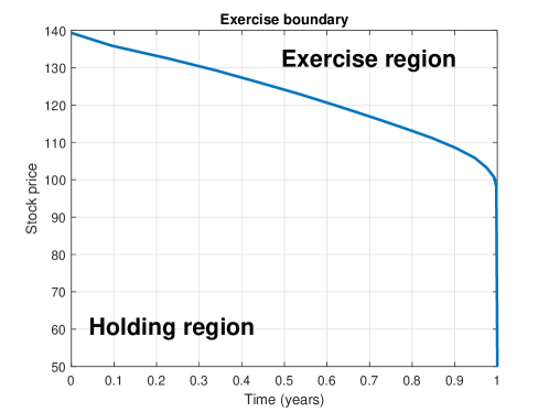
Figure 1: Typical exercise boundary for the American Call option under the Black-Scholes model with $K=50,r=0.2,q=0.1,\sigma=0.5,T=1$.

By a standard argument, [Cont and Voltchkova,, 2005, Klebaner,, 2005] the Call option price $C(S,t)$ in the continuation area solves a parabolic partial differential equation (PDE)

$$\frac{\partial C}{\partial t}+\frac{\displaystyle 1}{\displaystyle 2}\sigma^{2}(t)\frac{\partial^{2}C}{\partial S^{2}}+[r(t)-q(t)]S\frac{\partial C}{\partial S}=r(t)C.$$ (2)

subject to the terminal condition at the option maturity $t=T$

$$C(T,S)=(S-K)^{+},$$ (3)

and the boundary conditions

$$C(t,0)=0,\qquad\Delta(t,S_{B}(t))=1,\qquad\Delta(t,S)=\frac{\partial C(t,S)}{\partial S}.$$ (4)

Note, that for the arithmetic Brownian Motion process the domain of definition is $S\in(-\infty,\infty)$, however here we move the boundary condition from minus infinity to zero, see [Itkin and Muravey,, 2020] about rigorous boundary conditions for this problem. This is because in practice we can control the left boundary to make the probability of $S$ dropping below 0 to be low.

Further let us assume that the exercise boundary is somehow known. Then $C(S,t)$ can be found by solving Eq. 2 subject to the terminal condition in Eq. 3 and the boundary conditions

$$C(t,0)=0,\qquad C(t,S_{B}(t))=S_{B}(t)-K.$$ (5)

In other words, the American option price $C(S,t)$ in this region concises with the price of a double barrier option with the same maturity $T$, strike $K$, the constant lower barrier $L=0$ with no rebate at hit, and the time-dependent upper barrier $H=S_{B}(t)$. When the upper barrier is reached, the option is terminated, and the option holder gets a rebate at hit in the amount $S_{B}(t)-K$.

Obviously, in the exercise region the undiscounted Call option value is $C(t,S)=(S-K)^{+}\mathds{1}_{S\geq S_{B}(t)}$, where $\mathds{1}_{x}$ is the indicator function.

Below across this entire paper and for all presented models we assume that the pricing problem for the corresponding barrier option can be solved semi-analytically as this is shown in [Itkin et al.,, 2021, Itkin and Muravey, 2022b, , Carr et al.,, 2022]. Accordingly, our main focus here will be on i) deriving an integral equation for the exercise boundary $S_{B}(t)$ for each model considered in the paper, and ii) developing efficient methods (semi-analytical or numerical) for solving these integral equations.

Another comment should be made about using the GIT technique for solving the problems in this paper. Since all the problems have a vanishing terminal condition, a method of Heat potentials (HP) can also be used for doing so, [Itkin et al.,, 2021]. However, the HP method would be more expensive in this case as compared with the GIT. That is, because in the HP method we first express the solution via the heat potential density $\Omega(\tau)$ and obtain an integral Volterra equation which $\Omega$ solves. Then, another integral expression of the gradient of the solution at the moving boundary is obtained, in more detail [Itkin et al.,, 2021], Chapter 8. Thus, instead of a single Volterra equation as for the GIT, here we need to solve a system of two Volterra equations, hence this method is less efficient.

1.1.1 Nonlinear integral Volterra equation for $S_{B}(t)$

In [Carr and Itkin,, 2021] the PDE in Eq. 2 by a series of transformations has been reduced to the heat equation

$$\frac{\partial u}{\partial\tau}=\frac{\partial^{2}u}{\partial x^{2}},\qquad(\tau,x)\in\mathbb{R}_{+}\times[0,y(\tau)],\qquad y(\tau)=S_{B}(t(\tau))g(t(\tau)),\\$$ (6)

which should be solved subject to the terminal condition

$$u(0,x)=\left(xg(T)-K\right)^{+}e^{-f(T,x)},$$ (7)

and the boundary conditions

$$u(\tau,0) =0,\qquad u(\tau,y(\tau))=y(\tau)-K.$$ (8)

Here, first a change of independent variables was made

$$x =Sg(t),\qquad g(t)=e^{\int_{T}^{t}w(s)ds},\qquad\tau(t)=\frac{1}{2}\int_{t}^{T}\sigma^{2}(s)e^{2\int_{0}^{s}w(m)\,dm}\,ds,$$ (9)

(so, $y(\tau)=S_{B}(t(\tau))g(t(\tau))$), where the function $w(t)$ solves the Riccati equation

$$w^{\prime}(t)=2(r(t)-q(t))\frac{\sigma^{\prime}(t)}{\sigma(t)}-\left[(r(t)-q(t))^{2}+r^{\prime}(t)-q^{\prime}(t)\right]+w(t)^{2}+2w(t)\frac{\sigma^{\prime}(t)}{\sigma(t)},$$ (10)

followed by a change of the dependent variable

$$u(\tau,x) =C(S,t(\tau))e^{-f(t(\tau),x)},$$ (11)

$$f(t,x) =\frac{1}{2}\log\left(\frac{g(t)}{g(T)}\right)+\frac{1}{2}\int_{T}^{t}[3r(s)-q(s)]ds-\frac{g^{\prime}(t)+g(t)(r(t)-q(t))}{2g(t)^{3}\sigma(t)^{2}}x^{2}.$$

The Riccati equation in Eq. 10 cannot be solved analytically for arbitrary functions $r(t),q(t),\sigma(t)$, but can be efficiently solved numerically. Also, in some cases it can be solved in closed form, see [Carr and Itkin,, 2021].

Since the holding region is defined as $(\tau,x)\in[0,\tau(0)]\times[0,y(\tau)]$ (this is the area under the exercise boundary curve in Fig. 1) and $g(0)=1,\ y(0)=K$ , the terminal condition in Eq. 7 becomes homogeneous, i.e.

$$u(0,x)=0.$$ (13)

Thus, the Eq. 6 is a PDE with the homogeneous initial condition and the boundary condition at $x=0$ and an inhomogeneous boundary condition at $x=y(\tau)$. It turns out that this problem has been already solved in [Itkin and Muravey, 2022a, ] where pricing problem of double barrier options was investigated in detail. In terms of that paper, our problem in Eq. 6 can be treated as a pricing problem for the double barrier option with the lower barrier $y_{B}(\tau)=0$ and the upper barrier $z_{B}(\tau)=y(\tau)$ and also rebates paid at hit. The boundary conditions (rebates) at these barriers accordingly are

$$f^{-}(\tau)\equiv u(\tau,y_{B}(\tau))=0,\qquad f^{+}(\tau)\equiv u(\tau,z_{B}(\tau))=y(\tau)-K.$$ (14)

It is worth mentioning that this problem by a change ov variables $U(\tau,x)=u(\tau,x)-\frac{x}{y(\tau)}f^{+}(\tau)$ can be transformed to a similar problem, but with all terminal and boundary conditions to be homogeneous

$$\frac{\partial U}{\partial\tau} =\frac{\partial^{2}U}{\partial x^{2}}+\lambda(\tau,x),\qquad\lambda(\tau,x)=-x\frac{\partial}{\partial\tau}\left(\frac{f^{+}(\tau)}{y(\tau)}\right),$$ (15)

$$U(0,x) =U(\tau,0)=U(\tau,y(\tau))=0.$$

Then the Duhamel’s principle can be applied to solve this problem if the solution of the same problem but with no source term is known.

The solution of [Itkin and Muravey, 2022a, ] applied to our problem in Eq. 6 reads

$$u(\tau,x) =\int_{0}^{\tau}\Psi(s,y(s))B_{0}(x,\tau\,|\,y(s),s)+\int_{0}^{\tau}\int_{0}^{y(s)}\lambda(s,\xi)B_{0}(x,\tau\,|\,\xi,s)d\xi ds+\frac{x}{y(\tau)}f^{+}(\tau),$$

$$\Psi(\tau,y(\tau)) =-\frac{y(\tau)-K}{y(\tau)}+\frac{\partial u(\tau,x)}{\partial x}\Bigg{|}_{x=y(\tau)},$$ (16)

$$B_{0}(x,\tau\,|\,\xi,s) =\sum_{n=-\infty}^{\infty}\Upsilon_{n}(x,\tau\,|\,\xi,s),\qquad\Upsilon_{n}(x,\tau\,|\,\xi,s)=\frac{1}{2\sqrt{\pi(\tau-s)}}\left[e^{-\frac{(2ny(\tau)+x-\xi)^{2}}{4(\tau-s)}}-e^{-\frac{(2ny(\tau)+x+\xi)^{2}}{4(\tau-s)}}\right].$$

In what follows we will also need the following function

$$B_{1}(x,\tau\,|\,\xi,s) =\sum_{n=-\infty}^{\infty}\Lambda_{n}(x,\tau\,|\,\xi,s),$$ (17)

$$\Lambda_{n}(x,\tau\,|\,\xi,s) =\frac{\partial}{\partial\xi}\Upsilon_{n}(x,\tau\,|\,\xi,s)=\frac{x-\xi+2ny(\tau)}{4\sqrt{\pi(\tau-s)^{3}}}e^{-\frac{(2ny(\tau)+x-\xi)^{2}}{4(\tau-s)}}+\frac{x+\xi+2ny(\tau)}{4\sqrt{\pi(\tau-s)^{3}}}e^{-\frac{(2ny(\tau)+x+\xi)^{2}}{4(\tau-s)}}.$$

Note that the Fourier series in these expressions usually converge rapidly when $n$ grows. Similarly, taking the derivative of this series on $x$ provides a convenient way of calculating the corresponding derivative $\frac{\partial u(\tau,x)}{\partial x}$, [Olver et al.,, 2020].

An alternative representation can be obtained in terms of the Jacobi theta functions of the third kind $\theta_{3}(z,\omega)$, [Mumford et al.,, 1983]

$$B_{0}(x,\tau\,|\,\xi,s) =\frac{1}{2y(\tau)}\left[\theta_{3}(\phi_{-}(x,\xi,\tau),\omega_{2}(s,\tau))-\theta_{3}(\phi_{+}(x,\xi,\tau),\omega_{2}(s,\tau))\right],$$ (18)

$$B_{1}(x,\tau\,|\,\xi,s) =-\frac{\pi}{4y(\tau)^{2}}\left[\theta^{\prime}_{3}(\phi_{-}(x,\xi,\tau),\omega_{2}(s,\tau))+\theta^{\prime}_{3}(\phi_{+}(x,\xi,\tau),\omega_{2}(s,\tau))\right].$$

Here

$$\theta_{3}(z,\omega) =1+2\sum_{n=1}^{\infty}\omega^{n^{2}}\cos(2nz),\quad\omega_{1}(s,\tau)=e^{-\left(\frac{\pi\sqrt{s}}{y(\tau)}\right)^{2}},\quad\omega_{2}(s,\tau)=e^{\left(\frac{\pi\sqrt{s-\tau}}{y(\tau)}\right)^{2}},$$ (19)

$$\phi_{-}(x,z,\tau) =\frac{\pi(x-z)}{2y(\tau)},\quad\phi_{+}(x,z,\tau)=\frac{\pi(x+z)}{2y(\tau)}.$$

A well-behaved theta function must have parameter $|\omega|<1$, [Mumford et al.,, 1983]. This condition holds for any $\tau>0$. Also, $\theta^{\prime}_{3}(x,\omega)$ is the first derivative of the Jacobi Theta function on $x$ (e.g., EllipticThetaPrime in Wolfram Mathematica).

The formulas Section 1.1.1 and Eq. 18 are complementary. Since the exponents in Eq. 18 are proportional to the difference $\tau-s$, the Fourier series Eq. 18 converge fast if $\tau-s$ is large. Contrary, the exponents in Section 1.1.1 are inversely proportional to $\tau-s$. Therefore, the series Section 1.1.1 converge fast if $\tau-s$ is small. As mentioned in [Itkin and Muravey, 2022a, ], this situation is well investigated for the heat equation with constant coefficients. There exist two representation of the solution: one - obtained by using the method of images, and the other one - by the Fourier series. Despite both solutions are equal as the infinite series, their convergence properties are different, [Lipton,, 2001].

It is easy to see that by definition, $\Psi(\tau,y(\tau))$ is the Call option Delta (shifted by $1-K/y(\tau)$ ) at the exercise boundary but expressed in new dependent and independent variables. Since in the original variables it is given by Eq. 4, it can be explicitly expressed in the new variables as well to obtain

$$u(\tau,y(\tau)) =\left[\frac{y(\tau)}{g(\tau)}-K\right]e^{-f(t(\tau),y(\tau))},$$ (20)

$$\Psi(\tau,y(\tau)) =-\frac{y(\tau)-K}{y(\tau)}+\frac{e^{-f(t(\tau),y(\tau))}}{g(\tau)}\left[1+y(\tau)\left(y(\tau)-Kg(\tau)\right)a(t(\tau))\right],$$

$$a(t(\tau)) =\frac{g^{\prime}(t)+g(t)(r(t)-q(t))}{g^{3}(t)\sigma(t)^{2}}.$$

Thus, Section 1.1.1, Eq. 18 provides a semi-analytic expression of the American Call option price if the exercise boundary $y(\tau)$ is known.

If $y(\tau)$ is not known, it can be found by solving a Volterra integral equation. At the first glance, it can be obtained by setting $x=y(\tau)$ in Section 1.1.1 and substitute the values of $u(\tau,y(\tau)),\Psi(\tau,y(\tau))$ from Eq. 20 into it. However, it can be verified that in this case $B_{0}(y(\tau),\tau\,|\,y(s),s)=B_{1}(y(\tau),\tau\,|\,y(s),s)=0$, i.e., Section 1.1.1 reduces to the correct boundary condition Eq. 14 at the moving boundary. Therefore, the right way of finding $y(\tau)$ is similar to how the Volterra equation for the unknown function $\Psi(\tau)$ is derived when using the GIT method. Both parts of Section 1.1.1 can be first, differentiated by $x$, and then $x=y(\tau)$ should be substituted into the result. This yields, [Itkin and Muravey, 2022a, ]

$$\Psi(\tau,y(\tau)) =-\int_{0}^{\tau}\Psi(s,y(s))\left[\frac{y(\tau)-y(s)}{2\sqrt{\pi(\tau-s)^{3}}}e^{-\frac{(y(\tau)-y(s))^{2}}{4(\tau-s)}}-\upsilon^{+}_{0}(\tau\,|\,s,y(s))\right]ds$$

$$+\int_{0}^{\tau}\int_{0}^{y(s)}\lambda(s,\xi)B_{1}(y(\tau),\tau\,|\,\xi,s)d\xi ds+\frac{1}{y(\tau)}f^{+}(\tau),$$ (21)

where

$$\upsilon^{+}_{0}(\tau\,|\,s,\xi) =\sum_{\begin{subarray}{c}n=-\infty\\ n\neq 0\end{subarray}}^{\infty}\frac{\xi-(2n+1)y(\tau)}{2\sqrt{\pi(\tau-s)^{3}}}e^{-\frac{(-\xi+(2n+1)y(\tau))^{2}}{4(\tau-s)}}.$$ (22)

An alternative representation can be obtained in terms of the Jacobi theta function $\theta_{3}(z,\omega)$

$$\upsilon^{+}_{0}(\tau\,|\,s,\xi) =\frac{\pi}{2y(\tau)^{2}}\theta^{\prime}_{3}\left(\phi_{-}(y(\tau),\xi,\tau),\omega_{2}(s,\tau)\right)+\frac{y(\tau)-\xi}{2\sqrt{\pi(\tau-s)^{3}}}e^{-\frac{(\xi-y(\tau))^{2}}{4(\tau-s)}}.$$ (23)

It can be checked that $f^{+}(0)=0$. Substituting these formulae into Section 1.1.1 and taking into account $f^{+}(\tau)=y(\tau)-K$ we arrive at the following replacement for Section 1.1.1

$$\Psi(\tau,y(\tau)) =-\int_{0}^{\tau}\Psi(s,y(s))\left[\frac{y(\tau)-y(s)}{2\sqrt{\pi(\tau-s)^{3}}}e^{-\frac{(y(\tau)-y(s))^{2}}{4(\tau-s)}}-\upsilon^{+}_{0}(\tau\,|\,s,y(s))\right]ds$$ (24)

$$+\int_{0}^{\tau}\int_{0}^{y(s)}\lambda(s,\xi)B_{1}(y(\tau),\tau\,|\,\xi,s)d\xi ds+\frac{1}{y(\tau)}f^{+}(\tau),$$

which by substituting the definitions from Eq. 23 takes a form

$$\Psi(\tau,y(\tau)) =\frac{1}{y(\tau)}f^{+}(\tau)+\frac{\pi}{2y(\tau)^{2}}\int_{0}^{\tau}\Psi(s,y(s))\theta^{\prime}_{3}\left(\phi_{-}(y(\tau),y(s),\tau),\omega_{2}(s,\tau)\right)ds$$ (25)

$$+\int_{0}^{\tau}\int_{0}^{y(s)}\lambda(s,\xi)B_{1}(y(\tau),\tau\,|\,\xi,s)d\xi ds.$$

Since $\lambda(\tau,x)$ in Eq. 15 is a linear function of $x$, the inner integral in the last term can be further simplified to yield

$$\int_{0}^{y(s)} \lambda(s,\xi)B_{1}(y(\tau),\tau\,|\,\xi,s)d\xi=-\frac{\partial}{\partial\tau}\left(\frac{f^{+}(\tau)}{y(\tau)}\right)\Bigg{\{}$$ (26)

$$\frac{1}{2y(\tau)}\left[\theta_{3}\left(\phi_{-}(y(\tau),y(s),\tau),\omega_{2}(s,\tau)\right)+\theta_{3}\left(\phi_{+}(y(\tau),y(s),\tau),\omega_{2}(s,\tau)\right)\right]$$

$$+\frac{1}{2}\sum_{n=-\infty}^{\infty}\left[\operatorname{Erf}\left(\frac{(2n+1)y(\tau)+y(s)}{2\sqrt{\tau-s}}\right)-\operatorname{Erf}\left(\frac{(2n+1)y(\tau)-y(s)}{2\sqrt{\tau-s}}\right)\right]\Bigg{\}}.$$ (27)

The Eq. 25 is nonlinear in $y(\tau)$ in contrast to a similar equation but w.r.t. $\Psi(\tau,y(\tau))$ which occurs when pricing barrier options, [Itkin et al.,, 2021]. Moreover, this is not a standard nonlinear Volterra integral equation, neither of the first nor of the second kind which by definition could be written in the form, [Polyanin and Manzhirov,, 2008]

$$\xi(\tau) =\int_{0}^{\tau}K(\tau,s,y(s))ds,$$ (28)

$$y(\tau) =\xi(\tau)+\int_{0}^{\tau}{\cal K}(\tau,s,y(\tau),y(s))ds,$$

respectively, where $\xi(\tau)$ is some arbitrary function of $\tau$. In contrast, the integral Volterra equations Eq. 24 can be represented in a general form

$$\xi(\tau,y(\tau))=\int_{0}^{\tau}K(\tau,s,y(s))ds.$$ (29)

Below in this paper we discuss how to solve Eq. 24 by using various methods also including those from machine learning (ML).

A short remark should be made that the dependencies like $a(t(\tau))$ can be computed by using some finite grid in $t\in[0,T]$ and then creating a map $t\to\tau\in[0,\tau(0)]$ according to the definition of $\tau(t)$ in Eq. 9. Since all these dependencies are analytic, this procedure doesn’t bring any computational problem. Also, as $\tau=0$ corresponds to $t=T$, it follows from Eq. 19 that $y(0)=S_{B}(T)g(T)=Kg(T)$ for the American Call option, while for the American Put this is $y(0)=g(T)\min(K,Kr(T)/q(T))$, [Kim,, 1990]

1.2 The time-dependent Hull-White model

This model was investigated in [Itkin and Muravey,, 2020] with a goal to construct semi-analytic prices of barrier options, in more detail see also [Itkin et al.,, 2021]. Therefore, in what follows we will borrow some results obtained in that paper. Historically, the model was introduced in [Hull and White,, 1990] to describe dynamics of the short interest rate $r_{t}$ as following the OU process with time-dependent coefficients

$$dr_{t}=\kappa(t)[\theta(t)-r_{t}]dt+\sigma(t)dW_{t},\qquad r_{t=0}=r.$$ (30)

Here $\kappa(t)>0$ is the constant speed of mean-reversion, $\theta(t)$ is the mean-reversion level. To address calibration to real market rate curves the model could be updated by using a deterministic shift $s(t)$, so $r(t)=s(t)+\bar{r}(t)$ where $\bar{(}t)$ solves Eq. 30. This, however, can be easily done within our framework, as this is described in [Itkin et al.,, 2021]. In the commodities world this model is known as one-factor Schwartz’s model, [Schwartz,, 1997], for the logarithm of the spot price $S$.

Since $r_{t}$ itself is not tradable, we consider a zero-coupon bond (ZCB) with the maturity $Q$ and the price $F(r,t,Q)$ as the underlying instrument and look at pricing of American options written on $F(r,t,Q)$, in particular, the American Put. A typical shape of the exercise boundary for the Put option is presented in Fig. 2.

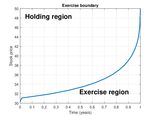
Figure 2: Typical exercise boundary for the American Put option under the Black-Scholes model with $K=50,r=0.2,q=0.1,\sigma=0.5,T=1$.

Using the same argument as in Section 1.1, let’s assume that the exercise boundary $F_{B}(t)$ is known. Then, in the continuation (holding) region the pricing problem for the American Put $P(t,r)$ is equivalent to pricing Down-and-Out barrier option at the domain $\Omega:r\in[F(r_{B}(t),t),\infty)\times t\in[0,T]$, with $T\leq Q$. It is known that in this region $F(r,t,Q)$ under a risk-neutral measure solves a linear parabolic partial differential equation (PDE), [Privault,, 2012, Itkin and Muravey,, 2020]

$$\frac{\partial F}{\partial t}+\frac{\displaystyle 1}{\displaystyle 2}\sigma^{2}(t)\frac{\partial^{2}F}{\partial r^{2}}+\kappa(t)[\theta(t)-r]\frac{\partial F}{\partial r}=rF.$$ (31)

subject to the terminal

$$F(r,Q,Q)=1,$$ (32)

and boundary conditions

$$F(0,t,Q)=g(t),\qquad F(r,t,Q)\Big{|}_{r\to\infty}=0,$$ (33)

where $g(t)$ is some function of the time $t$, see, e.g., [Zhang and Yang,, 2017] and references therein among others. However, since the Hull-White model belongs to the class of affine models, [Andersen and Piterbarg,, 2010], the solution of Eq. 31 can be represented in the form

$$F(r,t,Q) =A(t,Q)e^{B(t,Q)r},$$ (34)

$$B(t,Q) =e^{\int_{0}^{t}\kappa(x)\,dx}\int_{Q}^{t}e^{-\int_{0}^{x}\kappa(q)\,dq}\,dx,$$

$$A(t,Q) =\exp\left[-\frac{1}{2}\int_{Q}^{t}B(x,Q)\left(2\theta(x)\kappa(x)+B(x,Q)\sigma^{2}(x)\right)dx\right].$$

It can be seen that $B(t,Q)<0$ if $t<Q$. Therefore, $F(r,t,Q)\to 0$ when $r\to\infty$.

In turn, the American Put price $P(t,r)$ in the continuation region solves the PDE

$$\frac{\partial P}{\partial t}+\frac{\displaystyle 1}{\displaystyle 2}\sigma^{2}(t)\frac{\partial^{2}P}{\partial r^{2}}+\kappa(t)[\theta(t)-r]\frac{\partial P}{\partial r}=rP,\qquad(\tau,x)\in\mathbb{R}_{+}\times[y(\tau),\infty),$$ (35)

subject to the terminal condition

$$P(T,r)=\left(K-F(r,T,Q)\right)^{+},$$ (36)

the boundary condition at the moving boundary

$$P(t,r_{B}(t))=K-F(r_{B}(t),t,Q)=K-A(t,Q)e^{B(t,Q)r_{B}(t)},$$ (37)

and the other boundary condition at the second boundary at $r\to\infty$. Since based on Eq. 34 in this limit the ZCB price tends to zero, this yields

$$P(t,r)\Big{|}_{r\to\infty}=K.$$ (38)

1.2.1 Reduction to the heat equation

By changing the dependent variable

$$P(t,r)\to p(t,r)+K-F(r_{B}(t),t,Q),$$ (39)

we obtain a similar problem but with a homogeneous boundary conditions at the moving boundary, inhomogeneous boundary condition at infinity and a source term, namely:

$$\frac{\partial p}{\partial t} +\frac{\displaystyle 1}{\displaystyle 2}\sigma^{2}(t)\frac{\partial^{2}p}{\partial r^{2}}+\kappa(t)[\theta(t)-r]\frac{\partial p}{\partial r}=rp+\bar{\lambda}(t,r),$$ (40)

$$\bar{\lambda}(t,r) =r\left[K-F(r_{B}(t),t,Q)\right]+\partial_{t}F(r_{B}(t),t,Q).$$

This PDE has to be solved subject to the terminal condition

$$p(T,r)=\left(K-F(r,T,Q)\right)^{+}-K+F(r_{B}(T),T,Q)=0,$$ (41)

which is due to the fact that in the continuation region for the American Put option $\left(K-A(T,Q)e^{B(T,Q)r}\right)^{+}=0$, see Fig. 2, and also $A(T,Q)e^{B(T,Q)r_{B}(T)}=K$. Also, the boundary condition at the moving boundary becomes homogeneous

$$p(t,r_{B}(t))=0,$$ (42)

and the other boundary condition at infinity - inhomogeneous

$$p(t,r)\Big{|}_{r\to\infty}=F(r_{B}(t),t,Q).$$ (43)

This problem (with no source term $\lambda(t)$) has been already considered in [Itkin and Muravey,, 2020]. By transformations

$$p(t,r)=\exp[\alpha(t)r+\beta(t)]u(\tau,x),\qquad\tau=\phi(t),\qquad x=r\psi(t)+\xi(t),$$ (44)

it can be reduced to the heat equation with a source term

$$\frac{\partial u}{\partial\tau} =\frac{\partial^{2}u}{\partial x^{2}}+\tilde{\lambda}(\tau,x),$$ (45)

$$\tilde{\lambda}(\tau,x) =\frac{2\bar{\lambda}(t(\tau),r)}{\sigma^{2}(t)\psi^{2}(t)}\exp\left[-\beta(t)-\frac{\alpha(t)}{\psi(t)}(x-\xi(t))\right],\quad t=t(\tau),\quad\ r=\frac{x-\xi(t)}{\psi(t)},$$

that should be solved subject to the initial and boundary conditions

$$u(0,x) =0,\qquad u(\tau,y(\tau))=0,$$ (46)

$$u(\tau,x)\Big{|}_{x\to\infty} =A(t,Q)\exp[\frac{B(t,Q)-\alpha(t)}{\psi(t)}(y(\tau)-\xi(t))-\beta(t)]\equiv-g(\tau),\quad t=t(\tau).$$

Here $y(\tau)$ is the exercise boundary expressed in new variables $(\tau,x)$, i.e. $y(\tau)=\xi(t(\tau))+\psi(t)r_{B}(t(\tau))$.

The remaining notation in Eq. 45 reads

$$\psi(t) =\exp\left(\int_{0}^{t}\kappa(q)dq\right), \quad\phi(t) =\frac{1}{2}\int_{t}^{T}\sigma^{2}(q)\psi^{2}(q)dq,$$ (47)

$$\alpha(t) =\psi(t)\int_{0}^{t}\frac{1}{\psi(q)}dq, \quad\beta(t) =-\frac{1}{2}\int_{0}^{t}\alpha(q)\left[2\kappa(q)\theta(q)+\sigma^{2}(q)\alpha(q)\right]dq,$$

$$\xi(t) =-\int_{0}^{t}\left[\kappa(q)\theta(q)+\sigma^{2}(q)\alpha(q)\right]\psi(q)dq, \quad\tau(t) =\frac{1}{2}\int_{t}^{T}\sigma^{2}(q)\psi^{2}(q)dq.$$

Here $t(\tau)$ is the inverse map $t\rightarrow\tau$ which is found explicitly by solving the second equation in Eq. 47 with respect to $t$.

1.2.2 Nonlinear integral Volterra equation for $y(\tau)$

In this section we present a GIT based approach to derive a Volterra integral equation for the exercise boundary $y(\tau)$. For doing so, we start with a problem closely related to Eq. 45 but with different boundary conditions. By slightly changing the notation: $u(\tau,x)\mapsto U(\tau,x)$, we get

$$\frac{\partial U}{\partial\tau} =\frac{\partial^{2}U}{\partial x^{2}}+\lambda(\tau,x)\in\mathbb{R}_{+}\times(y(\tau),+\infty),$$ (48)

$$U(0,x) =f(x),\qquad U(\tau,y(\tau))=g(\tau),\quad U(\tau,x)\Big{|}_{x\to+\infty}=0.$$

Here the functions $g(\tau)$, $f(x),\lambda(\tau,x)$ and $y(\tau)$ are defined to guarantee the existence and uniqueness of the problem Eq. 48. By the change of variables

$$V(\tau,x)=U(\tau,x)-g(\tau)$$

we obtain the problem with absorbing boundary conditions (compare with Eq. 45)

$$\frac{\partial^{2}V}{\partial x^{2}} =\frac{\partial V}{\partial\tau}+g^{\prime}(\tau)-\lambda(\tau,x),\quad(\tau,x)\in\mathbb{R}_{+}\times(y(\tau),+\infty),$$ (49)

$$V(\tau,y(\tau)) =0,\quad V(\tau,x)\Big{|}_{x\to+\infty}=-g(\tau),$$

$$V(0,x) =f(x)-g(0),$$

By using the idea of GIT, let us consider a pair of integral transforms $\bar{v}_{\pm}$

$$\bar{v}_{\pm}(\tau,\omega)=\int_{y(\tau)}^{+\infty}e^{\pm\mathrm{i}\mkern 1.0mu\omega x}V(\tau,x)dx$$ (50)

and apply them to Eq. 49. We have

$$\int_{y(\tau)}^{+\infty}e^{\pm\mathrm{i}\mkern 1.0mu\omega x}\frac{\partial^{2}V(\tau,x)}{\partial x^{2}}dx =-\frac{\partial V(\tau,x)}{\partial x}\Big{|}_{x=y(\tau)}e^{\pm\mathrm{i}\mkern 1.0mu\omega y(\tau)}\mp\mathrm{i}\mkern 1.0mu\omega\int_{y(\tau)}^{+\infty}e^{\pm\mathrm{i}\mkern 1.0mu\omega x}\frac{\partial V(\tau,x)}{\partial x}dx=-\Psi(\tau,y(\tau))e^{\pm\mathrm{i}\mkern 1.0mu\omega y(\tau)}-\omega^{2}\bar{v}_{\pm},$$

$$\int_{y(\tau)}^{+\infty}e^{\pm\mathrm{i}\mkern 1.0mu\omega x}\frac{\partial V(\tau,x)}{\partial\tau}dx =\frac{d}{d\tau}\left[\int_{y(\tau)}^{+\infty}e^{\pm\mathrm{i}\mkern 1.0mu\omega x}V(\tau,x)dx\right]+e^{\pm\mathrm{i}\mkern 1.0mu\omega x}V(\tau,y(\tau))y^{\prime}(\tau)=\frac{d\bar{v}_{\pm}}{d\tau}.$$

Here the function $\Psi(\tau,y(\tau))$ is the gradient of the solution at the moving boundary $y(\tau)$

$$\Psi(\tau,y(\tau))=\frac{\partial V(\tau,x)}{\partial x}\Big{|}_{x=y(\tau)}.$$ (51)

Collecting all the terms together we obtain the ordinary differential equation (ODE) for $\bar{v}_{\pm}$

$$\frac{d\bar{v}_{\pm}(\tau,\omega)}{d\tau}+\omega^{2}\bar{v}_{\pm} =-\Psi(\tau,y(\tau))e^{\pm\mathrm{i}\mkern 1.0mu\omega y(\tau)}-g^{\prime}(\tau)\int_{y(\tau)}^{+\infty}e^{\pm\mathrm{i}\mkern 1.0mu\omega x}dx+\int_{y(\tau)}^{+\infty}e^{\pm\mathrm{i}\mkern 1.0mu\omega x}\lambda(\tau,x)dx$$ (52)

$$\bar{v}(0,\omega) =\int_{y(0)}^{+\infty}e^{\pm\mathrm{i}\mkern 1.0mu\omega x}(f(x)-g(0))dx.$$

Here $y(0)$ is the value of the exercise boundary at maturity, which for an American Put option is, [Karatzas and Shreve,, 1998]

$$y(0^{+})=\begin{cases}K,&r(0)\geq q(0),\\ \frac{r(0)}{q(0)}K,&r(0)<q(0).\end{cases}$$ (53)

Solving Eq. 52 by using a standard technique yields the explicit formula for $\bar{v}(\tau,\omega)$

$$\bar{v}_{\pm}(\tau,\omega) =e^{-\omega^{2}\tau}\int_{y(0)}^{+\infty}e^{\pm\mathrm{i}\mkern 1.0mu\omega x}(f(x)-g(0))dx$$ (54)

$$-\int_{0}^{\tau}e^{-\omega^{2}(\tau-s)}\left[\Psi(s,y(s))e^{\pm\mathrm{i}\mkern 1.0mu\omega y(s)}+g^{\prime}(s)\int_{y(s)}^{+\infty}e^{\pm\mathrm{i}\mkern 1.0mu\omega x}dx-\int_{y(s)}^{+\infty}\lambda(s,x)dx\right]ds.$$

To the best of our knowledge, each transform $\bar{v}_{+}$ and $\bar{v}_{-}$ is not explicitly invertible, however their linear combination is. Indeed,

$$\bar{v}(\tau,\omega)=\frac{\bar{v}_{+}e^{-\mathrm{i}\mkern 1.0mu\omega y(\tau)}-\bar{v}_{-}e^{+\mathrm{i}\mkern 1.0mu\omega y(\tau)}}{2\mathrm{i}\mkern 1.0mu}=\frac{1}{\mathrm{i}\mkern 1.0mu}\int_{y(\tau)}^{+\infty}V(\tau,x)\sinh\left[\mathrm{i}\mkern 1.0mu\omega(x-y(\tau))\right]dx$$

$$=\int_{y(\tau)}^{+\infty}V(\tau,x)\sin\left(\omega(x-y(\tau))\right)dx=\int_{0}^{+\infty}V(\tau,x+y(\tau))\sin\left(\omega x\right)dx$$

which is a sine transform with a well-known inversion formula. On the other hand, the function $\bar{v}(\tau,\omega)$ can be represented as following

$$\bar{v}(\tau,\omega) =e^{-\omega^{2}\tau}\int_{y(0)}^{+\infty}\sin\left[\omega(x-y(\tau))\right](f(x)-g(0))dx$$

$$-\int_{0}^{\tau}e^{-\omega^{2}(\tau-s)}\left[\Psi(s,y(s))\sin\left[\omega(y(s)-y(\tau))\right]+\int_{y(s)}^{+\infty}\left(g^{\prime}(s)-\lambda(s,x)\right)\sin\left[\omega(x-y(\tau))\right]dx\right]ds.$$

Integrating by parts and replacing $x$ by $\xi$ yields

$$\bar{v}(\tau,\omega) =e^{-\omega^{2}\tau}\int_{y(0)}^{+\infty}\sin\left[\omega(\xi-y(\tau))\right](f(\xi)-g(0))d\xi-\int_{0}^{\tau}e^{-\omega^{2}(\tau-s)}\Psi(s,y(s))\sin\left[\omega(y(s)-y(\tau))\right]ds$$

$$-g(\tau)\int_{y(\tau)}^{+\infty}\sin\left[\omega(\xi-y(\tau))\right]d\xi+g(0)e^{-\omega^{2}\tau}\int_{y(0)}^{+\infty}\sin\left[\omega(\xi-y(\tau))\right]d\xi$$

$$+\int_{0}^{\tau}g(s)\frac{d}{ds}\left[e^{-\omega^{2}(\tau-s)}\int_{y(s)}^{+\infty}\sin\left(\omega(\xi-y(\tau))\right)d\xi ds\right]$$

$$+\int_{0}^{\tau}e^{-\omega^{2}(\tau-s)}\int_{y(s)}^{+\infty}\lambda(s,x)\sin\left(\omega(\xi-y(\tau))\right)d\xi ds$$

$$=e^{-\omega^{2}\tau}\int_{y(0)}^{+\infty}\sin\left[\omega(\xi-y(\tau))\right]f(\xi)d\xi-\int_{0}^{\tau}e^{-\omega^{2}(\tau-s)}\Psi(s,y(s))\sin\left[\omega(y(s)-y(\tau))\right]ds$$

$$-g(\tau)\int_{y(\tau)}^{+\infty}\sin\left[\omega(x-y(\tau))\right]dx+\int_{0}^{\tau}g(s)\frac{d}{ds}\left[e^{-\omega^{2}(\tau-s)}\int_{y(0)}^{+\infty}\sin\left(\omega(\xi-y(\tau))\right)d\xi ds\right]$$

$$+\int_{0}^{\tau}e^{-\omega^{2}(\tau-s)}\int_{y(s)}^{+\infty}\lambda(s,\xi)\sin\left(\omega(\xi-y(\tau))\right)d\xi ds$$

Using the inversion formula for the sine transform

$$V(\tau,x)=\frac{2}{\pi}\int_{0}^{+\infty}\bar{v}(\tau,\omega)\sin\left[\omega(x-y(\tau))\right]d\omega.$$ (55)

we obtain

$$V(\tau,x) =\frac{2}{\pi}\int_{0}^{+\infty}\sin\left(\omega(x-y(\tau))\right)e^{-\omega^{2}\tau}\int_{y(0)}^{+\infty}\sin\left[\omega(\xi-y(\tau))\right]f(\xi)d\xi d\omega$$ (56)

$$-\frac{2}{\pi}\int_{0}^{+\infty}\sin\left(\omega(x-y(\tau))\right)\int_{0}^{\tau}e^{-\omega^{2}(\tau-s)}\Psi(s,y(s))\sin\left[\omega(y(s)-y(\tau))\right]dsd\omega$$

$$-\frac{2}{\pi}\int_{0}^{+\infty}\sin\left(\omega(x-y(\tau))\right)g(\tau)\int_{y(\tau)}^{+\infty}\sin\left[\omega(\xi-y(\tau))\right]d\xi d\omega$$

$$+\frac{2}{\pi}\int_{0}^{+\infty}\sin\left(\omega(x-y(\tau))\right)\int_{0}^{\tau}g(s)\frac{d}{ds}\left[e^{-\omega^{2}(\tau-s)}\int_{y(0)}^{+\infty}\sin\left(\omega(\xi-y(\tau))\right)d\xi ds\right]d\omega$$

$$+\frac{2}{\pi}\int_{0}^{+\infty}\sin\left(\omega(x-y(\tau))\right)\int_{0}^{\tau}\lambda(s,\xi)e^{-\omega^{2}(\tau-s)}\int_{y(0)}^{+\infty}\sin\left(\omega(\xi-y(\tau))\right)d\xi dsd\omega.$$

By changing the order of integration and applying well-known identities, [Gradshtein and Ryzhik,, 2007]

$$\int_{0}^{+\infty}e^{-\beta^{2}x}\sin(ax)\sin(bx)dx=\frac{1}{4}\sqrt{\frac{\pi}{\beta}}\left(e^{-\frac{(a-b)^{2}}{4\beta}}-e^{-\frac{(a+b)^{2}}{4\beta}}\right)$$

$$\frac{2}{\pi}\int_{0}^{+\infty}\sin\left(\omega(x-y(\tau))\right)\int_{y(\tau)}^{+\infty}\sin\left[\omega(\xi-y(\tau))\right]d\xi d\omega\equiv 1.$$

we arrive at the following formula

$$V(\tau,x)= -g(\tau)+\frac{1}{2\sqrt{\pi\tau}}\int_{y(0)}^{+\infty}f(\xi)\left[e^{-\frac{(\xi-x)^{2}}{4\tau}}-e^{-\frac{(\xi+x-2y(\tau))^{2}}{4\tau}}\right]d\xi$$

$$-\int_{0}^{\tau}\frac{\Psi(s,y(s))}{2\sqrt{\pi(\tau-s)}}\left[e^{-\frac{(x-y(s))^{2}}{4(\tau-s)}}-e^{-\frac{(x-2y(\tau)+y(s))^{2}}{4(\tau-s)}}\right]ds$$

$$+\int_{0}^{\tau}g(s)\left[\frac{d}{ds}\left(\frac{1}{2\sqrt{\pi(\tau-s)}}\int_{y(s)}^{+\infty}\left[e^{-\frac{(x-\xi)^{2}}{4(\tau-s)}}-e^{-\frac{(x-2y(\tau)+\xi))^{2}}{4(\tau-s)}}\right]d\xi\right)\right]ds$$

$$+\int_{0}^{\tau}\int_{y(s)}^{\infty}\frac{\lambda(s,\xi)}{2\sqrt{\pi(\tau-s)}}\left[e^{-\frac{(\xi-y(s))^{2}}{4(\tau-s)}}-e^{-\frac{(\xi-2y(\tau)+y(s))^{2}}{4(\tau-s)}}\right]d\xi ds$$

Substituting back $U=V+g(\tau)$ and doing some algebra yields

$$U(\tau,x) =\frac{1}{2\sqrt{\pi\tau}}\int_{y(0)}^{+\infty}f(\xi)\left[e^{-\frac{(\xi-x)^{2}}{4\tau}}-e^{-\frac{(\xi+x-2y(\tau))^{2}}{4\tau}}\right]d\xi$$

$$-\int_{0}^{\tau}\frac{\Psi(s,y(s))}{2\sqrt{\pi(\tau-s)}}\left[e^{-\frac{(x-y(s))^{2}}{4(\tau-s)}}-e^{-\frac{(x-2y(\tau)+y(s))^{2}}{4(\tau-s)}}\right]ds$$

$$+\int_{0}^{\tau}g(s)\left[\frac{d}{ds}\left(\frac{1}{2\sqrt{\pi(\tau-s)}}\int_{y(s)}^{+\infty}\left[e^{-\frac{(x-\xi)^{2}}{4(\tau-s)}}-e^{-\frac{(x-2y(\tau)+\xi))^{2}}{4(\tau-s)}}\right]d\xi\right)\right]ds$$

$$+\int_{0}^{\tau}\int_{y(s)}^{\infty}\frac{\lambda(s,\xi)}{2\sqrt{\pi(\tau-s)}}\left[e^{-\frac{(\xi-y(s))^{2}}{4(\tau-s)}}-e^{-\frac{(\xi-2y(\tau)+y(s))^{2}}{4(\tau-s)}}\right]d\xi ds$$

Again, integrating by parts in the last integral, we finally obtain

$$U(\tau,x) =\frac{1}{2\sqrt{\pi\tau}}\int_{y(0)}^{+\infty}f(\xi)\left[e^{-\frac{(\xi-x)^{2}}{4\tau}}-e^{-\frac{(\xi+x-2y(\tau))^{2}}{4\tau}}\right]d\xi$$ (57)

$$-\int_{0}^{\tau}\frac{\Psi(s,y(s))+y^{\prime}(s)g(s)}{2\sqrt{\pi(\tau-s)}}\left[e^{-\frac{(x-y(s))^{2}}{4(\tau-s)}}-e^{-\frac{(x-2y(\tau)+y(s))^{2}}{4(\tau-s)}}\right]ds$$

$$+\int_{0}^{\tau}\frac{g(s)}{4\sqrt{\pi(\tau-s)^{3}}}\left[(x-y(s))e^{-\frac{(x-y(s))^{2}}{4(\tau-s)}}+(y(s)+x-2y(\tau))e^{-\frac{(x+y(s)-2y(\tau))^{2}}{4(\tau-s)}}\right]ds$$

$$+\int_{0}^{\tau}\int_{y(s)}^{\infty}\frac{\lambda(s,\xi)}{2\sqrt{\pi(\tau-s)}}\left[e^{-\frac{(\xi-x)^{2}}{4(\tau-s)}}-e^{-\frac{(\xi-2y(\tau)+x)^{2}}{4(\tau-s)}}\right]d\xi ds.$$

Thus, Eq. 57 gives a closed form solution of the problem Eq. 48. It is worth noting that the last term in Eq. 45 can be considered as an application of the Duhamel’s principle to the problem Eq. 45. However, we didn’t find in the literature any reference to using the Duhamel’s formula for problems with moving boundaries.

To apply this result to our problem of pricing the American Put option in Eq. 45, we need to set

$$u(\tau,x) =V(\tau,x)=U(\tau,x)-g(\tau),\qquad f(x)=g(0),\qquad\lambda(\tau,x)=\tilde{\lambda}(\tau,x)-g^{\prime}(\tau),$$ (58)

where $g(\tau)$ is defined in Eq. 46. Accordingly, $f^{\prime}(x)=0$ and the first term in Eq. 57 vanishes. Also, we have from Eq. 40, Eq. 45, Eq. 46

$$\lambda(\tau,x) =\frac{2re^{-r\alpha(t)-\beta(t)}}{\sigma(t)^{2}\psi(t)^{2}}\Bigg{\{}K-F(r_{B}(t),t,Q)+e^{B(t,Q)r_{B}(t)}\left[f_{1}(\tau,y(\tau))e^{\alpha(t)(x-y(t))/\psi(t)}+f_{2}(\tau,y(\tau))\right]\Bigg{\}},$$

$$r =\frac{x-\xi(t)}{\psi(t)},\quad t=t(\tau),\quad r_{B}(t)=\frac{y(\tau)-\xi(t(\tau))}{\psi(t(\tau))}.$$

where expressions for $f_{1}(\tau,y(\tau)),f_{2}(\tau,y(\tau))$ are simple but bulky, so we are omitting them here. Therefore, the last integral in Eq. 57 simplifies since, e.g.,

$$\int_{y(s)}^{\infty}\frac{1}{2\sqrt{\pi(\tau-s)}}e^{-\frac{(\xi-x)^{2}}{4(\tau-s)}}d\xi =\frac{1}{2}\left[1+\operatorname{Erf}\left(\frac{x-y(s)}{2\sqrt{\tau-s}}\right)\right],$$

etc., (i.e., all the integrals of a product of $\lambda(s,\xi)$ and the Gaussian kernel are expressed in closed form via $\operatorname{Erf},\operatorname{Erfc},\operatorname{Erfi}$ functions).

Similarly to Eq. 24, the exercise boundary $y(\tau)$ solves a nonlinear Volterra integral equation, that can be obtained from Eq. 57 by differentiating both parts on $x$ and setting $x=y(\tau)$. This equation also connects the gradient at the moving boundary $\Psi(\tau,,y(\tau))$ and the exercise boundary $y(\tau)$. However, due to existing singularities in the integrals in Eq. 57 this procedure requires a special approach which is described in Appendix B. It is shown there that the corresponding (regularized) Volterra integral equation reads

$$\Psi(\tau,y(\tau)) =\int_{y(0)}^{\infty}f^{\prime}(\xi)\frac{e^{-\frac{(\xi-y(\tau))^{2}}{4\tau}}}{\sqrt{\pi\tau}}d\xi+\int_{0}^{\tau}\Psi(s,y(s))\frac{(y(\tau)-y(s))e^{-\frac{(y(\tau)-y(s))^{2}}{4(\tau-s)}}}{2\sqrt{\pi(\tau-s)^{3}}}ds-\int_{0}^{\tau}g^{\prime}(s)\frac{e^{-\frac{(y(\tau)-y(s))^{2}}{4(\tau-s)}}}{\sqrt{\pi(\tau-s)}}ds$$

$$+\int_{0}^{\tau}\int_{y(s)}^{\infty}\lambda(s,\xi)\frac{\xi-y(\tau)}{2\sqrt{\pi(\tau-s)^{3}}}e^{-\frac{(\xi-y(\tau))^{2}}{4(\tau-s)}}d\xi ds.$$ (59)

It can be checked that this equation does not contain singularities anymore. Since for the American option the function $\Psi(\tau,y(\tau))$ is known, Section 1.2.2 is another form of the non-linear Volterra equation to be solved in order to compute the exercise boundary $y(\tau)$ for the American Put option in the time-dependent Hull-White model.

Again, as applied to pricing of the American Put option in Eq. 45, based on Eq. 58 we have the first integral in Section 1.2.2 vanishing, and the last integral on $\xi$ can be taken in closed form, while for $\Psi(\tau,y(\tau)$ we have from Eq. 37, Eq. 44, Eq. 46

$$\Psi(\tau,y(\tau) =\frac{\partial V(\tau,x)}{\partial x}\Big{|}_{x=y(\tau)}=\frac{\partial u(\tau,x)}{\partial x}\Big{|}_{x=y(\tau)}=-A(t,Q)B(t,Q)e^{[B(t,Q)-\alpha(t)]r_{B}(\tau)-\beta(t)}=B(\tau,Q)g(\tau),$$

$$t =t(\tau),\quad r_{B}(t)=\frac{y(\tau)-\xi(\tau)}{\psi(\tau)}.$$ (60)

To conclude, given a) some time-dependent model for the underlying (e.g., the stock price), b) the corresponding pricing PDE for the American option written on this underlying which is valid in the continuation region, c) this PDE by a series of transformations can be reduced to the heat equation with moving boundaries, it follows that the exercise boundary solves an integral non-linear Volterra equation that can be derived by using the method described in this section.

1.3 The time-dependent Verhulst model

A slightly more sophisticated example of the proposed technique is pricing American options under the time-dependent Verhulst model. As applied to finance it was proposed in [Itkin et al.,, 2020] based on the observation that some popular short-term interest models have to be revisited and modified to better reflect market conditions during COVID-19 period. The model is a modification of the popular Black-Karasinski (BK) model, which is widely used by practitioners for modeling interest rates, credit, and commodities. This modification gives rise to the stochastic Verhulst model, which is well-known in the population dynamics and epidemiology as a logistic model.

The main idea behind the model is that since the BK model doesn’t support fat tails at the lower end, besides not being analytically tractable, we introduce its modified version of the form

$$dz_{t} =\kappa(t)[\bar{\theta}(t)-e^{z_{t}}]dt+\sigma(t)dW_{t},$$ (61)

$$r_{t} =s(t)+Re^{z_{t}},\qquad R=r_{0}-s(0),\qquad(t,z_{t})\in[0,T]\times(-\infty,\infty).$$

In other words, we modify the dynamics of the stochastic variable $z_{t}$ in Eq. 61 in the mean-reversion term by replacing $z_{t}$ with $e^{z_{t}}$.

In Eq. 61 $R$ is some constant with the same dimensionality as $r_{t}$, e.g., it can be $R=r(0)-s(0)$, T is the maturity. This model is similar to the Hull-White model, but preserves positivity of $r_{t}$ by exponentiating the OU random variable $z_{t}$. Because of that, usually practitioners add a deterministic function (shift) $s(t)$ to the definition of $r_{t}$ to address possible negative rates and be more flexible when calibrating the term-structure of the interest rates.

It can be seen, that at small $t$ $|z_{t}|\ll 1$, and so choosing $\bar{\theta}(t)=1+\theta(t)$ replicates the BK model in the linear approximation on $z_{t}$. Similarly, the choice $\bar{\theta}(t)=e^{\theta(t)}$ replicates the BK model at $z_{t}$ close the mean-reversion level $\theta(t)$. Thus, the Verhulst model acquires the properties of the BK model while is a bit more tractable, again in more detail see [Itkin et al.,, 2020, 2021].

By a change of variables Eq. 61 transforms to the stochastic Verhulst or stochastic logistic model, which are well-known in the population dynamics and epidemiology; see, e.g., [Verhulst,, 1838, Bacaer,, 2011, Giet et al.,, 2015] and references therein. In the past, several authors attempted to use this model in finance; see, e.g., [Chen,, 2010, Londono and Sandoval,, 2015, Halperin and Feldshteyn,, 2018]. In our case, the stochastic Verhulst equation has the form

$$d{\bar{r}}_{t} =k(t){\bar{r}}_{t}[{\tilde{\theta}}(t)-{\bar{r}}_{t}]dt+\sigma(t){\bar{r}}_{t}dW_{t},\qquad{\bar{r}}_{t}=\frac{r_{t}-s(t)}{r_{0}-s(0)}=e^{z_{t}}.$$ (62)

Accordingly, by Itô’s lemma and the Feynman–Kac formula any contingent claim written on the $r_{t}$ as the underlying (for instance, the price $F({\bar{r}},t,Q)$ of a ZCB with maturity $T$) solves the following PDE

$$0 =\frac{\partial F}{\partial t}+\frac{\displaystyle 1}{\displaystyle 2}\sigma^{2}(t){\bar{r}}^{2}\frac{\partial^{2}F}{\partial{\bar{r}}^{2}}+\kappa(t){\bar{r}}[{\tilde{\theta}}(t)-{\bar{r}}]\frac{\partial F}{\partial{\bar{r}}}-(s(t)+R{\bar{r}})F,$$ (63)

which should be solved subject to the terminal and boundary conditions

$$F({\bar{r}},Q,Q)=1,\qquad F({\bar{r}},t,Q)\Big{|}_{{\bar{r}}\to\infty}=0.$$ (64)

In general, $F({\bar{r}},t,Q)$ can be found e.g., by solving an integral Volterra equation derived in [Itkin et al.,, 2020]. However, in some cases a closed form expression can also be found. For instance, when $\kappa(t)=\kappa=const$, it was obtained in [Itkin et al.,, 2020] and reads

$$F(\tau,Q,w) e^{C_{a}(C_{a}-1)\tau-\int_{T}^{t(\tau)}s(k)dk}=1+e^{w/2}w^{-C_{\alpha}}\left[{\cal I}(\tau,w)+\frac{1}{\pi^{2}\Gamma(R/\kappa)}{\cal J}(\tau,w)\right],$$ (65)

$${\cal J}(\tau,w) =\int_{0}^{\infty}\omega\left[e^{-(\omega^{2}+1/4)\tau}-1\right]\sinh\left(2\pi\omega\right)\Gamma_{C_{\gamma}}^{-}(\omega)\Gamma_{C_{\gamma}}^{+}(\omega)\Gamma_{1-C_{\alpha}}^{-}(\omega)\Gamma_{1-C_{\alpha}}^{+}(\omega)W_{C_{\gamma},\mathrm{i}\mkern 1.0mu\omega}\left(w\right)\,d\omega,$$

$${\cal I}(\tau,w) =\sum_{k=0}^{K}\frac{e^{\left(\mu_{k}^{2}-\frac{1}{4}\right)\tau}}{k!}\frac{2\mu_{k}}{\Gamma\left(\frac{3}{2}-C_{\alpha}+\mu_{k}\right)}\frac{\Gamma_{C_{\gamma}}^{+}\left(\mathrm{i}\mkern 1.0mu\mu_{k}\right)\Gamma_{C_{\gamma}}^{-}\left(\mathrm{i}\mkern 1.0mu\mu_{k}\right)}{\Gamma(C_{\alpha}-C_{\gamma})}W_{C_{\gamma},\mu_{k}}\left(w\right).$$

Here $Q=Q(\tau)$, $W_{\kappa,\mu}(w),\,\Gamma(x)$ are the Whittaker and Gamma functions, [Abramowitz and Stegun,, 1964], $C_{\alpha}=const$ - a new parameter of the model that can be found by calibration of all the model parameters to market data , and the following change of variables has been made

$$w =\frac{2\kappa\phi(t)}{\sigma^{2}(0)}{\bar{r}},\quad\tau=\frac{1}{2}\int_{t}^{Q}\sigma^{2}(k)\,dk,\quad\phi(t)=e^{\int_{0}^{t}\left[C_{\alpha}\sigma^{2}(k)-\kappa{\tilde{\theta}}(k)\right]dk},\quad C_{\gamma}=\frac{\gamma(t)}{\kappa},\quad\mu_{k}=\frac{1}{2}-k-C_{\alpha}.$$ (66)

Also, in Eq. 65 $K$ denotes the number of poles of the Gamma function which depends on the value of $C_{\alpha}$ : if $C_{\alpha}\geq 1/2$, the integrand function has no poles, if $C_{\alpha}<1/2$ the number of the poles is $K=1+\left\lfloor\frac{1}{2}-C_{\alpha}\right\rfloor$, where $\lfloor x\rfloor$ is the floor of $x$.

1.3.1 Nonlinear integral Volterra equation for $y(\tau)$

Similar to Section 1.2, we consider an American option written on a zero-coupon bond $F({\bar{r}},t,Q)$. In the continuation (holding) region the pricing problem for the American Put $P(t,r)$ reads

$$\frac{\partial P}{\partial t} +\frac{\displaystyle 1}{\displaystyle 2}\sigma^{2}(t){\bar{r}}^{2}\frac{\partial^{2}P}{\partial{\bar{r}}^{2}}+\kappa(t){\bar{r}}[{\tilde{\theta}}(t)-{\bar{r}}]\frac{\partial P}{\partial{\bar{r}}}=(s(t)+R{\bar{r}})P,$$ (67)

$$P(T,{\bar{r}}) =\left(K-F({\bar{r}},T,Q)\right)^{+}=0,\qquad P(t,{\bar{r}}_{B}(t))=K-F({\bar{r}}_{B}(t),t,Q),\qquad P(t,{\bar{r}})\Big{|}_{{\bar{r}}\to\infty}=K.$$

Similar to the change of the dependent variable in Eq. 39 we do

$$P(t,r)\to p(t,r)+K-F({\bar{r}}_{B}(t),t,Q),$$ (68)

to obtain from Eq. 67

$$\frac{\partial p}{\partial t} +\frac{\displaystyle 1}{\displaystyle 2}\sigma^{2}(t){\bar{r}}^{2}\frac{\partial^{2}p}{\partial{\bar{r}}^{2}}+\kappa(t){\bar{r}}[{\tilde{\theta}}(t)-{\bar{r}}]\frac{\partial p}{\partial{\bar{r}}}=[s(t)+R{\bar{r}}]p+\bar{\lambda}(t,{\bar{r}}),$$ (69)

$$\bar{\lambda}(t,{\bar{r}}) =[s(t)+R{\bar{r}}]\left[K-F({\bar{r}}_{B}(t),t,Q)\right]+\partial_{t}F({\bar{r}}_{B}(t),t,Q),$$

$$p(T,{\bar{r}}) =0,\qquad p(t,{\bar{r}}_{B}(t))=0,\qquad p(t,{\bar{r}})\Big{|}_{{\bar{r}}\to\infty}=F({\bar{r}}_{B}(t),t,Q).$$

Using another transformation proposed in [Itkin et al.,, 2020]

$$p(t,{\bar{r}}) =e^{\frac{\kappa(t)}{\sigma^{2}(t)}{\bar{r}}+\int_{T}^{t}s(k)dk}u(\tau,y),\quad x=\log{\bar{r}}+\int_{0}^{t}\left[\frac{\sigma^{2}(k)}{2}-\kappa(k){\tilde{\theta}}(k)\right]dk,\quad\tau=\frac{1}{2}\int_{t}^{T}\sigma^{2}(k)dk,$$ (70)

this problem can be reduced to a simpler form

$$\frac{\partial u}{\partial\tau} =\frac{\partial^{2}u}{\partial x^{2}}+\left[\alpha(\tau)e^{x}+\beta(\tau)e^{2x}\right]u+\lambda(\tau,x),$$ (71)

$$\alpha(\tau) =\frac{2\gamma(t(\tau))}{\sigma^{2}(t(\tau))}e^{-\int_{0}^{t}\left[\frac{\sigma^{2}(k)}{2}-\kappa(k){\tilde{\theta}}(k)\right]dk},\qquad\beta(\tau)=-\frac{\kappa^{2}(t(\tau))}{\sigma^{4}(t(\tau))}e^{-\int_{0}^{t}\left[\sigma^{2}(k)-2\kappa(k){\tilde{\theta}}(k)\right]dk},$$

$$\gamma(t) =-R+\frac{\kappa^{2}(t){\tilde{\theta}}(t)}{\sigma^{2}(t)}+\frac{d}{dt}\left(\frac{\kappa(t)}{\sigma^{2}(t)}\right),\qquad\lambda(\tau,x)=\frac{2}{\sigma^{2}(t(\tau))}\bar{\lambda}(t(\tau),{\bar{r}}(x)),$$

$$u(0,{\bar{r}}) =0,\qquad u(\tau,y(\tau))=0,\qquad u(\tau,x)\Big{|}_{x\to\infty}=e^{-\frac{\kappa(t)}{\sigma^{2}(t)}{\bar{r}}(x)+\int_{0}^{\tau}s(k)dk}F(y(\tau),\tau,Q(\tau)).$$

Let us compare two problems in Eq. 71 and Eq. 49. They differ only by the existence of an extra source term $\left[\alpha(\tau)e^{x}+\beta(\tau)e^{2x}\right]u$ in the RHS of Eq. 49. However, it is known that the Duhamel’s principle still can be applied in this case as this is discussed in [Itkin et al.,, 2020]. Therefore, we can use the solution of Eq. 71 in Eq. 57 which will now have an extra term in the RHS

$$U(\tau,x) =\frac{1}{2\sqrt{\pi\tau}}\int_{y(0)}^{+\infty}f(\xi)\left[e^{-\frac{(\xi-x)^{2}}{4\tau}}-e^{-\frac{(\xi+x-2y(\tau))^{2}}{4\tau}}\right]d\xi$$ (72)

$$-\int_{0}^{\tau}\frac{\Psi(s,y(s))+y^{\prime}(s)g(s)}{2\sqrt{\pi(\tau-s)}}\left[e^{-\frac{(x-y(s))^{2}}{4(\tau-s)}}-e^{-\frac{(x-2y(\tau)+y(s))^{2}}{4(\tau-s)}}\right]ds$$

$$+\int_{0}^{\tau}\frac{g(s)}{4\sqrt{\pi(\tau-s)^{3}}}\left[(x-y(s))e^{-\frac{(x-y(s))^{2}}{4(\tau-s)}}+(y(s)+x-2y(\tau))e^{-\frac{(x+y(s)-2y(\tau))^{2}}{4(\tau-s)}}\right]ds$$

$$+\int_{0}^{\tau}\int_{y(s)}^{\infty}\frac{1}{2\sqrt{\pi(\tau-s)}}\left[e^{-\frac{(\xi-x)^{2}}{4(\tau-s)}}-e^{-\frac{(\xi-2y(\tau)+x)^{2}}{4(\tau-s)}}\right]\left\{\lambda(s,\xi)+\left[\alpha(s)e^{\xi}+\beta(s)e^{2\xi}\right]U(s,\xi)\right\}d\xi ds.$$

Therefore, in this case Eq. 72 is not a closed form solution anymore, but rather an integral equation for $U(\tau,x)$.

In a similar way a non-linear integral Volterra equation for the exercise boundary can be obtained from Section 1.2.2, which now also contains an extra term

$$\Psi(\tau,y(\tau)) =\int_{y(0)}^{\infty}f^{\prime}(\xi)\frac{e^{-\frac{(\xi-y(\tau))^{2}}{4\tau}}}{\sqrt{\pi\tau}}d\xi+\int_{0}^{\tau}\Psi(s,y(s))\frac{(y(\tau)-y(s))e^{-\frac{(y(\tau)-y(s))^{2}}{4(\tau-s)}}}{2\sqrt{\pi(\tau-s)^{3}}}ds-\int_{0}^{\tau}g^{\prime}(s)\frac{e^{-\frac{(y(\tau)-y(s))^{2}}{4(\tau-s)}}}{\sqrt{\pi(\tau-s)}}ds$$

$$+\int_{0}^{\tau}\int_{y(s)}^{\infty}\left\{\lambda(s,\xi)+\left[\alpha(s)e^{\xi}+\beta(s)e^{2\xi}\right]U(s,\xi)\right\}\frac{\xi-y(\tau)}{2\sqrt{\pi(\tau-s)^{3}}}e^{-\frac{(\xi-y(\tau))^{2}}{4(\tau-s)}}d\xi ds.$$ (73)

Since the gradient of the solution $\Psi(\tau,y(\tau))$ is known in closed form, the equations Eq. 72 and Section 1.3.1 form a system of two non-linear equations. By solving it, the American Put price in the continuation region and the exercise boundary can be found. Numerical solution can be constructed along the lines discussed below in Sections 2, 4, see also [Itkin et al.,, 2020]. However, since Eq. 72 is a two-dimensional equation, this method is less efficient compared to the other models considered in this paper.

2 Some intermediate comments

Two examples presented in Sections 1.1, 1.2 reveal some general steps necessary to apply the GIT approach originally developed for pricing barrier options in the time-dependent models, to pricing American options for the same models. Due to generality of these steps, in this section we concentrate reader’s attention at them also focusing on some important details.

The first comment is about a map between the barrier and American options. It was seen in Section 1.1 that pricing American Call options due to the corresponding boundary conditions can be transformed to pricing an Up-And-Out barrier option in the continuation region defined at the domain $\Omega:S\in[0,S_{B}(t)]\times t\in[0,T]$, see Fig. 1. In other words, the spatial domain for this problem has a moving (time-dependent) upper boundary. As the GIT method has been developed for solving this kind of problems in a semi-analytical manner, due to the above-mentioned similarity it can be naturally applied for pricing American options as well.

For the American Put option doing in a similar manner as in Section 1.2 one can reduce a pricing problem for the American option to that one for the Down-And-Out barrier option defined at the domain $\Omega:S\in[S_{B}(t),\infty]\times t\in[0,T]$, see Fig. 2. Again, the GIT method can be utilized to construct a semi-analytic solution of this problem as this was shown in [Itkin et al.,, 2021] and various papers of the authors referenced therein.

The second point to be emphasized has been already discussed in Introduction and is about the boundary condition at the exercise boundary $S_{B}(t)$. For barrier options this is usually either zero (so the contract is terminated at hit of the barrier), or some constant rebate paid either at hit or at option’s maturity. In contrast, for the American option the payoff at the exercise boundary is known and is either $C_{A}(S_{B}(t),t))=S_{B}(t)-K$ for the Call, and $P_{A}(S_{B}(t),t))=K-S_{B}(t)$ for the Put. Accordingly, the option Delta is also known and is either 1 for the Call, or -1 for the Put.

As has been demonstrated in Section 1.2, by a simple change of variables this problem can be reduced to that with homogeneous boundary conditions (to exactly mimic the settings considered in most of the problems in [Itkin et al.,, 2021]). The cost for doing so is that the pricing PDE now becomes inhomogeneous and acquires a source term, see Eq. 45. However, given the solution of the homogeneous PDE, the full solution of the corresponding inhomogeneous PDE can be found either directly by using the GIT method, or by using a generalized Duhamel’s principle, like this was done in Section 1.2.2.

It should be emphasized that, despite so far we described our method only for the time-dependent OU and Hull-White models, any other model where the pricing PDE can be reduced to the heat equation with a source term can be treated in the same way. For instance, pricing Amercian Call and Put options in the time-dependent Black-Scholes model can be done by first, reducing the pricing PDE in the continuation region to the form of Eq. 48, and then using the solution of this equation obtained in Eq. 57. All these models can be reversely obtained from the heat equation by using Lie group analysis, see [Olver,, 1993, Gazizov and Ibragimov,, 1998] among others.

The third point also has been already briefly discussed in Section 1.1.1 and is about a Volterra integral equation which the unknown exercise boundary $S_{B}(t)$ solves. In contrast to the barrier options where a similar Volterra equation is derived for the option Delta at the moving boundary and is linear in Delta, here Volterra equations for $S_{B}(t)$ are non-linear and also of a special form given in Eq. 29. To make it transparent we can slightly re-write Eq. 29 in a form

$$\xi(\tau,y(\tau))-\xi(\tau,y(0))=\int_{0}^{\tau}K(\tau,s,y(s))ds-\xi(\tau,y(0)),$$ (74)

and assuming the function $\xi(\tau,x)$ has all derivatives in $x$ to be finite, obtain from Tailor series in $x=y(\tau)$

$$\int_{0}^{\tau}K(\tau,s,y(s))ds-\xi(\tau,y(0))=\xi^{\prime}_{x}(\tau,x)\Big{|}_{x=y(0)}(y(\tau)-y(0))+\text{extra terms},$$ (75)

where, e.g., for the time-dependent OU model considered in Section 1.1: $y(0)=Kg(T)$. With no extra terms in the RHS, Eq. 75 has a standard form of the non-linear Volterra equation of the second kind, but extra terms add more complexity to this equation.

It is worth noticing that Eq. 29 can also be re-written in the standard form

$$y(\tau)=\xi_{1}(\tau)+\int_{0}^{\tau}K_{1}(\tau,s,y(s),y^{\prime}(s))ds,$$ (76)

with $K_{1}$ being the new kernel which, however, now also depends on $y^{\prime}(s)$. In our opinion, from numerical point of view this form is less preferable since computation of $y^{\prime}(s)$ in the kernel decreases an accuracy of any corresponding method.

The last portion of comments in this Section is devoted to traditional methods of solving non-linear integral equations. For instance, a straightforward approach of solving Eq. 25 written in the form of Eq. 29 could be as follows. Let us represent the unknown function $y(s)$ on a discrete grid in time $\Omega:s\in[0,\tau]$ with $M+1$ nodes equally distributed at $[0,\tau]$ with the step $\delta=\tau/M)$. Thus, instead of a continuous variable $y(s)$ we obtain a discrete vector $y_{i},\ i=0,\ldots,M$, such that $y_{0}=y(0)=Kg(T),\ y_{M}=y(\tau)$. The integral kernel in the RHS of Eq. 25 can be approximated on this grid by using some quadratures, e.g., the trapezoidal rule (to provide the final solution with the accuracy $O(\delta^{2})$). Then, for each value $\tau=j\delta,j\in[0,\ldots,M]$ at the grid $\Omega$ the Eq. 29 we obtain

$$0=\delta\sum_{i=0}^{j}K(j\delta,i\delta,y_{i})\left(1-\frac{1}{2}\mathbf{1}_{i=0}\mathbf{1}_{i=j}\right)-\xi(j\delta,y_{j}),$$ (77)

where $\mathbf{1}_{x}$ is the indicator function. This is a system on nonlinear algebraic equations w.r.t. the vector of unknown values $y_{1},\ldots,y_{j}$. Since $y_{0}$ is already known, it can be solved sequentially, first for $j=1$, then for $j=2$ as the value of $y_{1}$ is already known from the previous step, etc. For solving non-linear algebraic equations various standard method are available, see [Rheinboldt,, 1998, Benton,, 2018] among others. Various programming languages (Python, Matlab, etc.) contain standard packages for solving nonlinear systems of equations.

To achieve a better accuracy, high order quadratures can be used for the kernel’s approximation, e.g., the Simpson rule which allows finding the solution with the accuracy $O(\delta^{4})$. In this case again Eq. 76 can be solved sequentially, but only starting from $j>2$. For $j=1,2$ the equations in Eq. 76 have to be solved together as a system of two nonlinear equations.

To illustrate this approach, we use an example from [Carr and Itkin,, 2021] where without any loss of generality parameters of the time-dependent OU model are chosen in the following way

$$r(t)=r_{0}e^{-r_{k}t},\qquad q(t)=q_{0},\qquad\sigma(t)=\sigma_{0}e^{-\sigma_{k}t}.$$ (78)

Here $r_{0},q_{0},\sigma_{0},r_{k},\sigma_{k}$ are constants. With this model Eq. 10 can be solved analytically to yield

$$w(t)=q_{0}-r_{0}e^{-r_{k}t}-r_{k}e^{-2\frac{r_{0}}{r_{k}}e^{-r_{k}t}}/E_{1+2(q_{0}-\sigma_{k})/r_{k}}\left(-2\frac{r_{0}}{r_{k}}e^{-r_{k}t}\right),$$ (79)

where $E_{n}(z)$ is the exponential integral function $E_{n}(z)=\int_{1}^{\infty}e^{-zt}/t^{n}dt$, [Abramowitz and Stegun,, 1964].

We choose parameters of the model as they are presented in Table 1.

$r_{0},1/yr$	$q_{0},1/yr$	$\sigma_{0},USD/\sqrt{yr}$	$r_{k},1/yr$	$\sigma_{k},1/yr$	$T,yr$
0.02	0.03	2 $K$	0.01	5	1

Table 1: Parameters of the test.

Let us recall, that here $\sigma(t)$ is the normal volatility. Therefore, we choose its typical value by multiplying the log-normal volatility by the strike level $K$. Also, for the values of parameters given in Tab. 1, the last term practically vanishes, so in what follows we neglect it. Accordingly, from Eq. 9, Eq. 11 we find

$$g(t) =\exp\left[q_{0}(t-T)+\frac{r_{0}}{r_{k}}\left(e^{-r_{k}t}-e^{-r_{k}T}\right)\right],\quad f(x,t)=\frac{r_{0}}{r_{k}}\left(e^{-r_{k}T}-e^{-r_{k}t}\right).$$ (80)

We run the test for a set of strikes $K\in[50,55,60,65,70,75,80]$. In Fig. 3a the exercise boundaries for the American Call option computed by solving Eq. 25 using the trapezoid quadratures are presented as a function of the time $t$. For the initial guess the already computed value $y(t_{i-1})$ can be chosen, and the method typically converges within 3-4 iterations. The total elapsed time to compute $S_{B}(t)$ on a temporal grid: $t_{i}=i\Delta t,\ i\in[0,M],\ \Delta t=T/M$ for all strikes with $M=20$ is 0.33 sec in Matlab (fsolve) using two Intel Quad-Core i7-4790 CPUs, each 3.80 Ghz. Despite our Matlab code can be naturally vectorized, we didn’t do it since in this example we used a simple method which can be approved in many different ways, i.e., see below in this paper. Also, it is worth mentioning that Matlab neither contain an embedded code for the Jacobi theta function (but it can be found in a third-party file exchange), nor for the derivatives of the theta function. Therefore, we refined translation of the original Pascal procedure made in the AMath library, see [Batista,, 2019, Fenton and Gardiner-Garden,, 1984] and references therein, and equipped it with computation of the function derivatives. However, these functions are available in other languages, e.g., as a part of the python package mpmath, [Johansson,, 2007] or in Wolfram Mathematica.

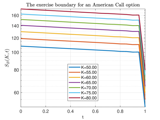
(a)

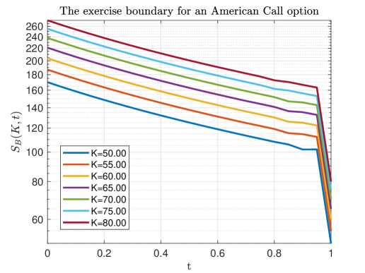
(b)

Figure 3: A semi-log plot of the exercise boundary $S_{B}(t)$ of the American Call option computed in the numerical example for various strikes $K\in[50:80]$; (a) parameters of the test are given in Table 1; (b) parameters of the test are given in Fig. 1.

Fig. 3b shows the results of the same test where parameters of the test are same as in Fig. 1 (so, $r_{K}=\sigma_{k}=0$. It can be seen that the exercise boundary is close to that presented in Fig. 1. The difference can be attributed to a difference in models (the OU vs the Black-Scholes model) because in this test the OU normal volatility $\sigma_{OU}$ is constant, and in the Black-Scholes model it is $\sigma_{BS}S$, i.e. a function of $S$, despite $\sigma_{OU}=\sigma_{BS}S$. Also, the elapsed time in the test at Fig. 1 is 0.05 sec per one strike, i.e. this is 0.35 sec for 7 strikes as in the test in this Section. Thus, the elapsed time in both tests is very close, despite here we used our semi-analytical method, and for the test in Fig. 1 - the trinomial tree. Note, that for the trinomial tree the number of discrete stock values was equal to the number of discrete time values which is 400, otherwise the accuracy of calculations is insufficient.

3 One-factor models that can be reduced to the Bessel equation

In this section we consider two typical examples of one-factor time-dependent models such that the American option pricing can be reduced to solving the Bessel equation at the time-dependent spatial domain. Again, we chose pricing of the American Call option written on a stock which follows the time-dependent CEV model, and pricing of the American Put option written on a zero-coupon bond where the underlying interest rate follows the time-dependent CIR model.

The pricing problem for barrier options where the underlying follows the CIR or CEV model was considered in [Carr et al.,, 2020]. The authors describe two approaches to solve it: a) generalization of the method of heat potentials for the heat equation to the Bessel process, (so we call it the method of Bessel potentials), and b) the GIT method also extended to the Bessel process. In all cases, a semi-analytic solution was obtained meaning that first, one needs to solve a linear Volterra integral equation of the second kind, and then the option price is represented as a one-dimensional integral. It was shown that computationally these methods are more efficient than both the backward and forward finite difference methods while providing better accuracy and stability. In more detail, see also [Itkin et al.,, 2021]. Here we use same methodology but for pricing American rather than barrier options.

3.1 The CEV model

The time-dependent constant elasticity of variance (CEV) model is a one-dimensional diffusion process that solves a stochastic differential equation (SDE)

$$dS_{t}=\mu(t)S_{t}dt+\sigma(t)S_{t}^{\beta+1}dW_{t},\qquad S_{t=0}=S_{0}.$$ (81)

Here $\mu(t)$ is the drift (under risk-neutral measure $\mu(t)=r(t)-q(t)$ where $r(t)$ is the deterministic short interest rate, and $q(t)$ is the continuous dividend), and $\beta$ is the elasticity parameter such that $\beta<1,\ \beta\neq\{0,-1\}$. The model with constant coefficients was first introduced in [Cox,, 1975] as an alternative to the geometric Brownian motion for modeling asset prices. We assume that all parameters of the model are known either as a continuous functions of time $t\in[0,\infty)$, or as a discrete set of $N$ values for some moments $t_{i},\ i=1,\ldots,N$.

For the standard CEV process with constant parameters the change of variable $z_{t}=1/(\sigma|\beta|)S_{t}^{-\beta}$ transforms the SDE Eq. 81 without drift ($\mu=0$) to the standard Bessel process of order $1/2\beta$, [Revuz and Yor,, 1999, Davydov and Linetsky,, 2001]). As shown in [Carr et al.,, 2020], a similar connection to the Bessel process can be established for the time-dependent version of the model in Eq. 81. The authors consider an Up-and-Out barrier Call option written on the underlying process $S_{t}$. By the same standard argument, [Cont and Voltchkova,, 2005, Klebaner,, 2005] its price $C(t,S)$ solves a parabolic PDE

$$\frac{\partial C}{\partial t}+\frac{\displaystyle 1}{\displaystyle 2}\sigma^{2}(t)S^{2\beta+2}\frac{\partial^{2}C}{\partial S^{2}}+[r(t)-q(t)]S\frac{\partial C}{\partial S}=r(t)C.,\qquad(t,S)\in[0,T]\times[0,S_{B}(t)].$$ (82)

By analogy already established in Section 1.1, the price $C(t,S)$ of the American Call option written on the same underlying, in the continuation region solves the same PDE Eq. 82. This equation should be solved subject to the terminal condition Eq. 3 and boundary conditions in Eq. 4. Again, we first solve this pricing problem semi-analytically assuming that the exercise boundary $S_{B}(t)$ is known, and then derive a nonlinear integral Volterra equation for $S_{B}(t)$ that needs to be solved numerically.

As it was already emphasize, $S_{B}(t)$ in the pricing problem for the American Call option corresponds to the upper barrier $H(t)$ for the Up-and-Out option, while the boundary conditions at the moving boundary differ, namely: for the American Call option we have $C(t,S_{B}(t))=S_{B}(t)-K$, while for the Up-and-Out barrier option this is $C(t,H(t))=0$ (if no rebate at hid is paid).

As shown in [Carr et al.,, 2020], by a set of transformations the problem Eq. 82, Eq. 3, Eq. 4 can be transformed to the Bessel PDE

Proposition 1 (Proposition 1.1 of [Carr et al.,, 2020]).

The PDE in Eq. 82 can be transformed to

$$\frac{\partial u}{\partial\tau}=\frac{1}{2}\frac{\partial^{2}u}{\partial z^{2}}+\frac{b}{z}\frac{\partial u}{\partial z},$$ (83)

where $b$ is some constant, $u=u(\tau,z)$ is the new dependent variable, and $(\tau,z)$ are the new independent variables. The Eq. 83 is the PDE associated with the one-dimensional Bessel process, [Revuz and Yor,, 1999]

$$dX_{t}=dW_{t}+\frac{b}{X_{t}}dt.$$ (84)

Here the transformation is done in two steps. The first change of variables reads

$$S=\left(-x\beta\right)^{-1/\beta},\qquad C(t,S)\to u(t,x)e^{\int_{T}^{t}r(k)dk},\qquad\phi=\int_{t}^{T}\sigma^{2}(k)dk,$$ (85)

and then the other change of variables is

$$z =xF(\phi),\quad\tau=\int_{0}^{\phi(t)}F^{2}(k)dk,\quad F(\phi)=e^{\int_{0}^{\phi}f(k)dk},\quad f(t)=\beta\frac{r(t)-q(t)}{\sigma^{2}(t)},\quad b=\frac{\beta+1}{2\beta}.$$ (86)

The PDE in Eq. 83 should be solved in the domain $(\tau,z)\in[0,\tau(0)]\times[0,y(\tau)]$ subject to the terminal condition (compare with Eq. 13)

$$u(0,z)=0,$$ (87)

and the boundary conditions

$$u(\tau,0)=0,\qquad u(\tau,y(\tau))=\left[y(\tau)^{-1/\beta}\left(\frac{\beta}{F(\phi(\tau))}\right)^{-1/\beta}-K\right]e^{-\int_{0}^{t(\tau)}r(k)dk}.$$ (88)

Another important value is the option Delta at the moving boundary $\Psi(\tau,z(\tau))=\frac{\partial u(\tau,z)}{\partial z}|_{z=z(\tau)}$ which can be found explicitly by using Proposition 1

$$\Psi(\tau,y(\tau))=\frac{1}{\beta}\left(\frac{F(\phi(\tau))}{\beta}\right)^{1/\beta}e^{-\int_{0}^{t(\tau)}r(k)dk}[-y(\tau)]^{-1-1/\beta}.$$ (89)

As mentioned in [Carr et al.,, 2020], the above formulae are valid at $-1<\beta<0$. However, if $0<\beta<1$, the left boundary goes to $-\infty$. Therefore, in this case it is convenient to redefine $x\to\bar{x}=-x$. This also redefines $z\to\bar{z}=-z$. Then the domain of definition for $\bar{z}$ becomes $\bar{z}\in[\bar{y}(\tau),\infty),\ \bar{y}(\tau)=-y(\tau)$. One can also observe that by changing the sign of the strike $\bar{K}=-K$ we obtain a pricing problem for the American Put option. The initial condition for this problem remains the same as in Eq. 87, the boundary condition at the moving boundary - same as in Eq. 88, but with the change $K\to\bar{K},\ y(\tau)\to\bar{y}(\tau)$. And, as usual, a vanishing boundary condition for the Put option at $z\to\infty$ is natural to be set as well. Also, in case $0<\beta<1$ the PDE in Eq. 83 keeps the same form in the $\bar{z}$.

3.2 The CIR model

As applied to pricing barrier options the time-dependent Cox–Ingersoll–Ross (CIR) model was considered in [Carr et al.,, 2020], so below we extract the main facts about this model from that paper. The original (time-independent) CIR model has been invented in [Cox et al.,, 1985] for modeling interest rates. In our time-dependent settings the CIR instantaneous interest rate $r_{t}$ follows the stochastic differential equation (SDE)

$$dr_{t}=\kappa(t)[\theta(t)-r_{t}]dt+\sigma(t)\sqrt{r_{t}}dW_{t},\qquad r_{t=0}=r.$$ (90)

Here $\kappa(t)>0$ is the speed of mean-reversion, $\theta(t)$ is the mean-reversion level. This model eliminates negative interest rates if the Feller condition $2\kappa(t)\theta(t)/\sigma^{2}(t)>1$ is satisfied, while still preserves tractability, see e.g., [Andersen and Piterbarg,, 2010] and references therein.

Since the CIR model belongs to the class of exponentially affine models, the price of the ZCB $F(r,t,Q)$ for this model is known in closed form. It is known, that $F(r,t,Q)$ under a risk-neutral measure solves a linear parabolic partial differential equation (PDE), [Privault,, 2012]

$$\frac{\partial F}{\partial t}+\frac{\displaystyle 1}{\displaystyle 2}\sigma^{2}(t)r\frac{\partial^{2}F}{\partial r^{2}}+\kappa(t)[\theta(t)-r]\frac{\partial F}{\partial r}=rF,$$ (91)

which should be solved subject to the terminal condition

$$F(r,Q,Q)=1,$$ (92)

and the boundary condition

$$F(r,t,Q)\Big{|}_{r\to\infty}=0.$$ (93)

The second boundary condition is necessary in case the Feller condition is violated, so the interest rate $r_{t}$ can hit zero. Otherwise, the PDE in Eq. 91 itself at $r=0$ serves as the second boundary condition.

The ZCB price can be obtained from Eq. 91 assuming that the solution is of the form

$$F(r,t,Q)=A(t,Q)e^{B(t,Q)r},$$ (94)

where $A(t,Q),B(t,Q)$ solve the system

$$\frac{\partial B(t,Q)}{\partial t} =1+\kappa(t)B(t,Q)-\frac{1}{2}\sigma^{2}(t)B^{2}(t,Q),\quad B(Q,Q)=0,$$ (95)

$$\frac{\partial A(t,Q)}{\partial t} =-A(t,Q)B(t,Q)\theta(t)\kappa(t),\quad A(Q,Q)=1.$$

The first equation in Eq. 95 is the Riccati equation. It this general form it cannot be solved analytically for arbitrary functions $\kappa(t),\sigma(t)$, but can be efficiently solved numerically. Also, in some cases it can be solved approximately (asymptotically), see e.g., an example in [Carr and Itkin,, 2021]. Once the solution is obtained, the second equation in Eq. 95 can be solve analytically to yield

$$A(t,Q)=e^{-\int_{Q}^{t}B(m)\theta(m)\kappa(m)\,dm}.$$ (96)

When coefficients $\kappa(t),\theta(t),\sigma(t)$ are constants, it is known that the solution $B(t,Q)$ can be obtained in closed form and reads, [Andersen and Piterbarg,, 2010]

$$B(t,Q)=-\frac{2[\exp((Q-t)h)-1]}{2h+(\theta+h)[\exp((Q-t)h)-1]},\qquad h=\sqrt{\theta^{2}+2\sigma^{2}}.$$ (97)

Thus, $B(t,Q)<0$ if $t<Q$. Therefore, $F(r,t,Q)\to 0$ when $r\to\infty$. In other words, the solution in Eq. 94 satisfies the boundary condition at $r\to\infty$. In case when all the parameters of the model are deterministic functions of time, and $B(t,Q)$ solves the first equation in Eq. 95, this also remains to be true, [Carr et al.,, 2020].

Our focus here is on pricing an American Put option written on a ZCB. Similar to Section 1.2 and [Carr et al.,, 2020] we observe that under a risk-neutral measure the option price $C(t,r)$ in the continuation region solves the same PDE as in Eq. 91, [Andersen and Piterbarg,, 2010].

$$\frac{\partial C}{\partial t}+\frac{\displaystyle 1}{\displaystyle 2}\sigma^{2}(t)r\frac{\partial^{2}C}{\partial r^{2}}+\kappa(t)[\theta(t)-r]\frac{\partial C}{\partial r}=rC,\quad(t,r)\in[0,T]\times[r(t),\infty),$$ (98)

where $r_{B}(t)$ is the exercise boundary. The terminal condition at the option maturity $T\leq Q$ for this PDE reads

$$C(T,r)=\left(K-F(r,T,S)\right)^{+}=0,$$ (99)

and the boundary conditions are same as in Eq. 37, Eq. 38.

3.2.1 Reduction to the Bessel equation

The PDE in Eq. 98 can also be transformed to that for the Bessel process in Eq. 84.

Proposition 2 (Proposition 2.1 of [Carr et al.,, 2020]).

The Eq. 98 can be transformed to

$$\frac{\partial u}{\partial\tau}=\frac{1}{2}\frac{\partial^{2}u}{\partial z^{2}}+\frac{b}{z}\frac{\partial u}{\partial z},$$ (100)

where $b=m-1/2$ is some constant, $u=u(\tau,z)$ is the new dependent variable, and $(\tau,z)$ are the new independent variables, if

$$\frac{\kappa(t)\theta(t)}{\sigma^{2}(t)}=\frac{m}{2},$$ (101)

where $m\in[0,\infty)$ is some constant. The Eq. 100 is the PDE associated with the one-dimensional Bessel process in Eq. 84.

Here the following transformations were used

$$C(t,r) =u(\tau,z)e^{a(t)r+\int_{T}^{t}a(s)\kappa(s)\theta(s)ds},\qquad z=g(t)\sqrt{r},\qquad t=t(\tau)$$ (102)

$$g(t) =\exp\left[\frac{1}{2}\int_{0}^{t}\left(\kappa(s)-a(s)\sigma^{2}(s)\right)\,ds\right],\qquad\tau(t)=\frac{1}{4}\int_{t}^{T}g^{2}(s)\sigma^{2}(s)\,ds,$$

where $a(t)$ solves the Riccati equation

$$\frac{da(t)}{dt}=-\frac{\sigma^{2}(t)a^{2}(t)}{2}+\kappa(t)a(t)+1.$$ (103)

The function $t(\tau)$ is the inverse map defined by the last equality in Eq. 102. It can be computed for any $t\in[0,T]$ by substituting it into the definition of $\tau$, then finding the corresponding value of $\tau(t)$, and inverting.

As follows from Proposition 2, for the time-dependent CIR model the transformation from Eq. 98 ro Eq. 100 cannot be done unconditionally. However, from practitioners’ points of view the condition Eq. 101 seems not to be too restrictive, Indeed, the model parameters already contain the independent mean-reversion rate $\kappa(t)$ and volatility $\sigma(t)$. Since $m$ is an arbitrary constant, it could be calibrated to the market data together with $\kappa(t)$ and $\sigma(t)$. Therefore, in this form the model should be capable for calibration to the term-structure of interest rates, again in more detail see [Carr et al.,, 2020].

In new variables the terminal and boundary conditions for Eq. 100 read

$$u(0,z) =0,\qquad u(\tau,z)\Big{|}_{z\to\infty}=0,\qquad u(\tau,y(\tau))=K-A(t,Q)e^{B(t,Q)g^{-2}(t)y^{2}(\tau)},\qquad t=t(\tau).$$ (104)

3.3 Nonlinear integral Volterra equation for $y(\tau)$

Let us, for example, consider the CEV model with $-1<\beta<0$, so by the Proposition 1 the pricing PDE in the continuation region can be transformed to the Bessel PDE Eq. 83 with a homogeneous terminal condition Eq. 87 and the boundary conditions Eq. 88. Let us compare this problem with a similar one for the time-dependent OU model which was solved in Section 1.1.1. It can be observed that both problems look similar, namely: they both have a homogeneous terminal condition and the boundary condition at $x=0$, and the other boundary condition at the moving boundary $y(\tau):u(\tau,y(\tau))=f^{+}(\tau)$, where $f^{+}(\tau)$ is some continuous function of $\tau$. Thus, those two problems differ only by the PDE itself: in for the OU model this is a heat equation Eq. 6 while for the CEV model this is a Bessel equation Eq. 83.

Based on our result obtained in [Carr and Itkin,, 2021] and replicated in Section 1.1.1, the solution of Eq. 6 with the corresponding terminal and boundary conditions can be represented via the following ansatz

$$u(\tau,x) =\int_{0}^{\tau}\Psi(s,y(s))B_{0}(x,\tau\,|\,y(s),s)+\int_{0}^{\tau}\int_{0}^{y(s)}\lambda(s,\xi)B_{0}(x,\tau\,|\,\xi,s)d\xi ds+\frac{x}{y(\tau)}f^{+}(\tau),$$ (105)

$$B_{0}(x,\tau\,|\,\xi,s) =\frac{1}{2y(\tau)}\left[\theta_{3}(\phi_{-}(x,\xi,\tau),\omega_{2}(s,\tau))-\theta_{3}(\phi_{+}(x,\xi,\tau),\omega_{2}(s,\tau))\right].$$

Here $\theta_{3}(\phi_{-}(x,\xi,\tau),\omega_{2}(s,\tau))$ and $\theta_{3}(\phi_{+}(x,\xi,\tau),\omega_{2}(s,\tau))$ are two periodic solutions of the heat equation in "conjugate" variables , [Mumford et al.,, 1983]

$$\frac{\partial}{\partial s}\theta_{3}(\phi_{\pm}(x,\xi,\tau),\omega_{2}(s,\tau))=-\frac{1}{4}\frac{\partial^{2}}{\partial\xi^{2}}\theta_{3}(\phi_{\pm}(x,\xi,\tau),\omega_{2}(s,\tau)).$$ (106)

The difference of two Green’s functions in the definition of $B_{0}(x,\tau\,|\,y(s),s)$ is necessary to obey the boundary conditions (like in the method of images, [Tikhonov and Samarskii,, 1963].

Constructing the solution in such a way and explaining this construction in such a form is useful because it allows a natural generalization of this approach. In particular, as applied to the problem in Eq. 82 with the terminal and boundary conditions in Eq. 87, Eq. 88, by analogy one can claim that the solution of this problem is also given by Eq. 105, where now a periodic solution of the heat equation has to be replaced with a periodic solution of the Bessel equation.

Fortunately, such a periodic solution has been already constructed in [Carr et al.,, 2020, Itkin and Muravey, 2022b, ]. In that paper we introduced a new function which we call the Bessel Theta function

$$\Theta_{\nu}(\theta,x_{1},x_{2})=\frac{2}{y(\tau)}(x_{1}x_{2})^{|\nu|}\sum_{n=1}^{\infty}e^{-\mu_{n}^{2}\theta^{2}}\frac{{J_{-\nu}}(\mu_{n}x_{1}){J_{-\nu}}(\mu_{n}x_{2})}{J_{|\nu|+1}^{2}(\mu_{n})}.$$ (107)

Here $J_{\nu}(x)$ is the Bessel function of the first kind, $\nu=1/(2\beta)<0$, since $\beta<0$, $\mu_{n}$ is an ordered sequence of positive zeros of the Bessel function ${J_{|\nu|}}(\mu)$:

$$J_{|\nu|}(\mu_{n})=J_{|\nu|}(\mu_{m})=0,\quad\mu_{n}>\mu_{m}>0,\quad n>m.$$

The function $\Theta_{\nu}(\theta,x_{1},x_{2})$ is an analog of the Jacobi theta function (which is a periodic spatial solution of the heat equation) in case of the Bessel equation.

It can be seen that at $\beta=-1,\nu=-1/2$ and $|\nu|=1/2$, our CEV problem becomes a time-dependent OU problem considered in Section 1.1.1. Therefore, taking into account that at $\nu=-1/2$, we have, [Abramowitz and Stegun,, 1964]

$$J_{-\nu}(x) =\sqrt{\frac{2}{\pi x}}\sin(x),\qquad\mu_{n}=n\pi,\ n=0,1,...$$

$$\Theta_{\nu} \left(\frac{\sqrt{\tau-s}}{y(\tau)},\frac{y(s)}{y(\tau)},\frac{x}{y(\tau)}\right)=\frac{2}{y(\tau)}\sqrt{\frac{y(s)}{y(\tau)}\frac{x}{y(\tau)}}\sum_{n=1}^{\infty}e^{-\frac{\mu_{n}^{2}(\tau-s)}{y^{2}(\tau)}}\frac{{J_{-\nu}}(\mu_{n}y(s)/y(\tau)){J_{-\nu}}(\mu_{n}x/y(\tau))}{J_{|\nu|+1}^{2}(\mu_{n})}$$

$$=\frac{2}{y(\tau)}\sum_{n=1}^{\infty}e^{-\frac{\mu_{n}^{2}(\tau-s)}{y^{2}(\tau)}}\frac{\pi^{2}n\sqrt{\frac{ny(s)}{y(\tau)}}\sqrt{\frac{nx}{y(\tau)}}\sin\left(\frac{\pi ny(s)}{y(\tau)}\right)\sin\left(\frac{\pi nx}{y(\tau)}\right)}{[\sin(\pi n)-\pi n\cos(\pi n)]^{2}\sqrt{\frac{xy(s)}{y(\tau)^{2}}}}$$

$$=\frac{1}{y(\tau)}\left[\sum_{n=1}^{\infty}\omega_{2}(s,\tau)^{n^{2}}\cos\left(\frac{\pi n(x-y(s))}{y(\tau)}\right)-\sum_{n=1}^{\infty}\omega_{2}(s,\tau)^{n^{2}}\cos\left(\frac{\pi n(y(s)+x)}{y(\tau)}\right)\right]$$

$$=\frac{1}{2y(\tau)}\left[\theta_{3}(\phi_{-}(x,\xi,\tau),\omega_{2}(s,\tau))-\theta_{3}(\phi_{+}(x,\xi,\tau),\omega_{2}(s,\tau))\right]=B_{0}(x,\tau\,|\,\xi,s).$$

Therefore, in this limit we restore the correct solution of Eq. 6 given in Section 1.1.1.

The sum in the definition number of $\Theta_{\nu}(...)$ usually quickly converges due to the exponential term. For instance, in Fig. 4 a difference between $\Theta_{\nu}\left(\frac{\sqrt{\tau-s}}{y(\tau)},\frac{y(s)}{y(\tau)},\frac{x}{y(\tau)}\right)$ and $B_{0}(x,\tau\,|\,\xi,s)$ is presented by using a test function $y(s)=5-\left(\frac{1}{2}+s\right)^{2}$, and the values $s=0.5,\tau=1$, and the sum is over $n\in[-M,M],\,M=10$.

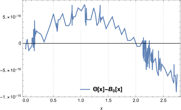
Figure 4: Convergence of $Theta_{\nu}(x)$ with $\nu=-0.5,\ s=0.5,\ \tau=1$, the sum is over $n\in[-M,M],\ M=10$, and $B_{0}(x,\tau\,|\,y[s],s)$ is computed in Wolfram Mathematica by using function EllipticTheta(3,z,q)|.

In Fig. 5 we also present a 3D plot of $\Theta_{\nu}\left(\frac{\sqrt{\tau-s}}{y(\tau)},\frac{y(s)}{y(\tau)},\frac{x}{y(\tau)}\right)$ as a function of $(x,s)$ obtained in the same experiment for 3 values of $\nu=1/(2\beta)$: $\beta=-1,-1/2,-0.1$.

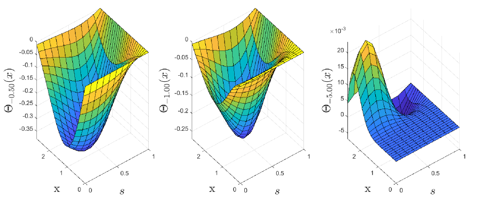
Figure 5: 3D plot of $\Theta_{\nu}\left(\frac{\sqrt{\tau-s}}{y(\tau)},\frac{y(s)}{y(\tau)},\frac{x}{y(\tau)}\right)$ as a function of $(x,s)$ obtained in the same experiment for three values of $\nu=1/(2\beta)$: $\beta=-1,-1/2,-0.1$.

Thus, using this analogy, we can represent the solution of Eq. 83 as

$$u(\tau,x) =\frac{x}{y(\tau)}f^{+}(\tau)+\int_{0}^{\tau}\Psi(s,y(s))\Theta_{\nu}\left(\frac{\sqrt{\tau-s}}{y(\tau)},\frac{y(s)}{y(\tau)},\frac{x}{y(\tau)}\right)ds$$ (108)

$$+\int_{0}^{\tau}\int_{0}^{y(s)}\lambda(s,\xi)\Theta_{\nu}\left(\frac{\sqrt{\tau-s}}{y(\tau)},\frac{\xi}{y(\tau)},\frac{x}{y(\tau)}\right)d\xi ds.$$

Here the function $f^{+}((s)$ is given by Eq. 88 and reads

$$f^{+}((s)=\left[y(s)^{-1/\beta}\left(\frac{\beta}{F(\phi(s))}\right)^{-1/\beta}-K\right]e^{-\int_{0}^{t(s)}r(k)dk}.$$ (109)

The gradient $\Psi(s,y(s))$ is also known explicitly and is given in Eq. 89.

Accordingly, the nonlinear integral Volterra equation for the exercise boundary $y(\tau)$ has the same form as Eq. 24, where now we need to replace the theta function $\theta_{3}\left(\phi_{-}(y(\tau),y(s),\tau),\omega_{2}(s,\tau)\right)$ and its derivatives with

$$\frac{1}{y(\tau)}\theta_{3}\left(\phi_{-}(y(\tau),y(s),\tau),\omega_{2}(s,\tau)\right) \mapsto\Theta_{-\nu}\left(\frac{\sqrt{\tau-s}}{y(\tau)},\frac{y(s)}{y(\tau)},1\right)+\Theta_{\nu}\left(\frac{\sqrt{\tau-s}}{y(\tau)},\frac{y(s)}{y(\tau)},1\right)+1,$$

$$\frac{\pi}{2y(\tau)^{2}}\theta^{\prime}_{3}\left(\phi_{-}(y(\tau),y(s),\tau),\omega_{2}(s,\tau)\right) \mapsto\frac{\partial}{\partial z}\Bigg{\{}\Theta_{-\nu}\left(\frac{\sqrt{\tau-s}}{y(\tau)},\frac{y(s)}{y(\tau)},z\right)+\Theta_{\nu}\left(\frac{\sqrt{\tau-s}}{y(\tau)},\frac{y(s)}{y(\tau)},z\right)\Bigg{\}}\Bigg{|}_{z=1}.$$

$$B_{1}(y(\tau),\tau\,|\,\xi,s) \mapsto\frac{1}{y(\tau)}\frac{\partial}{\partial z}\Theta_{\nu}\left(\frac{\sqrt{\tau-s}}{y(\tau)},\frac{\xi}{y(\tau)},z\right)\Bigg{|}_{z=1}$$ (110)

$$=2\xi^{|\nu|}y^{|\nu|-2}(\tau)\sum_{n=1}^{\infty}e^{-\frac{\mu^{2}_{n}(\tau-s)}{y(\tau)^{2}}}\frac{J_{-\nu}\left(\frac{\mu_{n}\xi}{y(\tau)}\right)}{J_{|\nu|+1}(\mu_{n})^{2}}\Big{[}(|\nu|+\nu)J_{-\nu}(\mu_{n})+\mu_{n}J_{-\nu-1}(\mu_{n})\Big{]},$$

This yields

$$\Psi(\tau,y(\tau)) =\frac{1}{y(\tau)}f^{+}(\tau)+\int_{0}^{\tau}\Psi(s,y(s))B_{1}(y(\tau),\tau\,|\,y(s),s)ds+\int_{0}^{\tau}\int_{0}^{y(s)}\lambda(s,\xi)B_{1}(y(\tau),\tau\,|\,\xi,s)d\xi ds.$$ (112)

Since by Eq. 15

$$\lambda(\tau,x)=-x\frac{\partial}{\partial\tau}\left(\frac{f^{+}(\tau)}{y(\tau)}\right),$$

and from Eq. 88

$$f^{+}(\tau)=\left[y(\tau)^{-1/\beta}\left(\frac{\beta}{F(\phi(\tau))}\right)^{-1/\beta}-K\right]e^{-\int_{0}^{t(\tau)}r(k)dk}$$

the inner integral in the last line of Eq. 112 can be further simplified, since

$$\int_{0}^{y(s)} \xi^{|\nu|+1}J_{-\nu}\left(\frac{\mu_{n}\xi}{y(\tau)}\right)\,d\xi=$$

$$-\frac{2^{\nu}y^{|\nu|+2}(s)}{[-|\nu|+\nu-2]\Gamma(1-\nu)}\left(\frac{\mu_{n}^{2}y(s)^{2}}{y(\tau)^{2}}\right)^{-\nu/2}\,_{1}F_{2}\left(-\frac{\nu}{2}+\frac{|\nu|}{2}+1;1-\nu,-\frac{\nu}{2}+\frac{|\nu|}{2}+2;-\frac{\mu_{n}^{2}y(s)^{2}}{4y(\tau)^{2}}\right),$$

where ${}_{1}F_{2}\left(a_{1};b_{1},b_{2};,z\right)$ is the generalized hypergeometric function, [Abramowitz and Stegun,, 1964].

This fully solves the problem under consideration. For the other interval $x\in[y(\tau),\infty)$ the solution can be constructed in the same way, and we leave it for the reader. Also, a method of solving a linear Volterra equation for the CEV and CIR models as well as computation of $\Theta_{\pm\nu}$ function are discussed in detail in [Carr et al.,, 2020]. Same approach can be used here for solving the corresponding nonlinear Volterra equation, also see the advanced discussion in the next Section.

4 Solving nonlinear Volterra equations by various methods including ML

In this Section we discuss various methods to solve non-linear non-standard integral Volterra equations of the type Eq. 28. Traditional method for solving non-linear equations of this type could be conventionally split into three groups, see e.g., a recent paper [Nedaiasl et al., 2019b, ] and references therein.

If the expression under the integral (the non-linear integral kernel) doesn’t have singularities, then direct quadratures can be used to approximate the integral term. The term $y^{\prime}(s)$ under the integral can be approximated by using finite differences of the necessary order of approximation. Thus obtained non-linear algebraic equation for $y(s)$ can be solved numerically using any standard method (e.g., the Newton-Raphson method) sequentially starting from $s=0$ and the $s=1,\ldots,M$. For doing so, one can build a discrete grid in time $\Omega:s\in[0,\tau]$ with $M+1$ nodes equally distributed at $[0,\tau]$ with the step $\delta=\tau/M)$. Then, instead of a continuous variable $y(s)$ we obtain a discrete vector $y_{i},\ i=0,\ldots,M$, such that $y_{0}=y(0)=K,\ y_{M}=y(\tau)$. Alternatively, a system of non-linear algebraic equations for the entire vector $y(0),\ldots,y(M)$ can be solved given some good initial guess.

Another possible form of this method can be constructed based on the observation that all the Volterra equations we need to solve, e.g., Eq. 25, are linear in $\Psi(\tau,y(\tau)$. Since the connection between $\Psi(\tau,y(\tau)$ and $y(\tau)$ is analytic (see, e.g, Eq. 20 or Section 1.2.2), the algorithm, e.g., for Eq. 25 could be as follows. Given the initial guess for $y(s),\ s=0,\ldots,M$, one can compute the kernels $\theta^{\prime}_{3}\left(\phi_{-}(y(\tau),y(s),\tau),\omega_{2}(s,\tau)\right)$ and the second integral in the RHS. of Eq. 25. This gives rise to a linear integral Volterra equation of the second kind for $\Psi(\tau,y(\tau)$. Once the solution is found on the grid (by using any standard method), new values of $y_{i},\ i=0,\ldots,M$ can be found by solving Eq. 20 w.r.t. to $y_{i}$. Then the iterations can be continued until necessary convergence is achieved.

In case the integral kernel contains some week (integrated) singularities, like in Section 1.2.2 which contains week singularities $(\tau-s)^{-1/2}$, a barycentric interpolation method can be used to resolve this, so the integral can we well approximated on the grid with no singularities in the final solution, in more detail see [Nedaiasl et al., 2019b, ].

Another class of methods that can be used for solving non-linear integral equation of the type Eq. 28 are interpolation or collocation-based methods. The idea of these methods is to approximate the continuous solution onto a finite-dimensional subspace. This can be done by using various polynomial or polynomial-spectral collocation procedures, e.g. see [Andersen et al.,, 2016] among others. Note that the approach of [Driscoll et al.,, 2014] implemented in the chebfun package in Matlab, where piecewise polynomial interpolants and Chebyshev polynomials are used for functional representation of objects, also belongs to this class. The package aims to combine the feel of symbolic computing systems like Maple and Mathematica with the speed of floating-point numerics, and also includes an API for solving nonlinear Volterra equations with high precision.

In [Carr et al.,, 2022] a three-dimensional integral Volterra (linear) equation was solved by approximating the kernel with the Radial Basis Functions (RBF) as this was proposed in [Assari et al.,, 2019, Zhang et al.,, 2014, Itkin and Muravey, 2022b, ] (see also references therein). In doing so, we proposed a new set of RBFs which allow computation of one integral (out of three) in closed form. It is proved that these new RBF can be used for interpolation and the corresponding analysis is provided in the paper. We then compare performance of our method with that of a modern FD approach and find that the former outperforms the later.

A recent paper [Lu et al.,, 2023] exploits the same idea but wrapped out into a ML framework. In more detail, the authors construct a new neural network (NN) method to solve linear Volterra and Fredholm integral equations based on the sine-cosine basis functions and extreme learning machine (ELM) algorithm. The NN consists of an input layer, a hidden layer, and an output layer, in which the hidden layer is eliminated by utilizing the sine-cosine basis functions. Furthermore, the problem of finding network parameters is converted into solving a set of linear equations.

Looking at this method, it is clear that the choice of the basis is not limited to just sine and cosine functions. The best choice of the basis should be that one which allows computation of the integral in the Volterra equation in closed form. For linear equations and simple kernels this can be done relatively easy. However, for nonlinear equations this could be either impossible at all (hence, instead the integral has to be computed numerically). or can be extremely bulky. Again, out trick of switching from non-linear equation for $y(\tau)$ to a linear one for $\Psi(\tau,y(\tau)$ given the current values of $y_{i}$ can help here, so this method can now be undoubtedly used, but it still requires iterations to converge. Once the expansion of $\Psi(\tau,y(\tau)$ into series of basis functions is found (all coefficients are computed), the value of $y(\tau)$ can also be easily computed by inverting (either analytically or numerically) the map $\Psi(\tau,y(\tau)\mapsto y(\tau)$.

The main advantages of interpolation-based methods lies in the fact that once interpolation coefficients are found, the approximate solution $y(s)$ can be obtained at any point $s\in[0,\tau(0)]$, in contrast to the direct quadratures method where the solution is known only in the grid points. A possible cost one has to pay for this is the speed of the method. But as usual for the ANN methods, the problem can be trained offline, so using the already trained ANN the solution can be obtained very fast.

For time-dependent models calibration of the model (training the ANN) could be a complex problem. Indeed, following [Itkin,, 2020] consider a financial model $\mathcal{M}$ with parameters of the model $p_{1},\ldots,p_{n},\ p_{i}\in\mathbb{R},n\in\mathbb{Z},n\geq 1$ which provides prices of some financial instruments given the input data $\theta_{1},\ldots,\theta_{l},\ l\in\mathbb{Z},l\geq 1$. For example, the OU model described in Section 1 has three time-dependent parameters $r(t),q(t),\sigma(t)$, and three input parameters $S,K,T$. The ANN approach for option pricing basically assumes that the ANN can be used as a universal approximator $\mathbb{R}^{n+l}\to\mathbb{R}$, i.e. given a vector of the input data $\bm{\theta}$ and a vector of the values of the model parameters $\bm{p}$ it provides a unique option price, e.g., the Call option price $C(\bm{\theta},\bm{p})$. Since parameters of the model are time-dependent, these time dependencies have to be described either analytically (hence, then constant parameters of this dependencies become new (additional) parameters of the entire model), or by another ANN trained accordingly to the market data. Once this is done, the whole model can be trained either to the available market data (thus, the model calibration is embedded into this step), or to the "reference" solutions of the corresponding integral Volterra equation. The "reference" solution, which is an output of the training samples, can then be obtained by using the other (e.g., direct) methods. The trained ANN then can be used for pricing American options for both in-sample and out-of-sample data.

Perhaps, this approach is too expensive to apply it to simple one-dimensional problems when the number of Volterra equations to be solved is small. However, with the increase of dimensionality, e.g. for stochastic volatility models or for basket options, it could be optimal. However, then speed-wise it should be compared with a similar ML approach applied directly to solving a corresponding PDE in the continuation region.

5 Conclusions

In this paper we demonstrate how the GIT technique could be extended from semi-analytic pricing of barrier options, [Itkin et al.,, 2021] to that for American options. Using as example some one-factor time-dependent models for the underlying, we describe in detail how the corresponding non-linear integral Volterra equation for the exercise boundary can be derived for both Call and Put options. To the best of our knowledge, before this result was known only for the Black-Scholes model with constant coefficients. We also provide some examples how thus obtained non-linear Volterra equations can be solved numerically.

To underline, in the paper we obtain semi-analytic representations of American options prices for the time-dependent models where the pricing PDE can be reduced either to the Heat or Bessel equation with a general source term and moving boundaries. The corresponding solutions in the continuation region are obtained analytically by using the GIT technique, however, the final result can be also treated as an application of the Duhamel’s principle to the corresponding problem. We believe this is also an interesting contribution, since we didn’t find in the literature any reference to using the Duhamel’s formula for problems with moving boundaries.

Moreover, we provide a roadmap how other similar PDEs can be solved in the same manner. The idea, e.g., for the domain $x\in[0,y(\tau)]$, is that when pricing American options the terminal and boundary conditions are the same for any model and read $u(0,x)=u(\tau,0)=0,\ u(\tau,y(\tau))=f^{+}(\tau)$, but the PDE themselves could differ. However, once a periodic solution of this PDE with fully homogeneous conditions (i.e., with $u(\tau,y(\tau))=0$ as well) is known, it can be plugged into the general ansatz of the solution given in Eq. 105 to provide the solution of the original problem. Same is true for the nonlinear integral Volterra equation solved by $y(\tau)$, which can be obtained in the same way, for instance, from Eq. 25.

Since the GIT approach can also be applied to pricing options under various stochastic volatility models, [Itkin and Muravey, 2022b, , Carr et al.,, 2022], by analogy it is expected that the same method can be used for American options as well. Currently, this is our work in progress.

Disclaimer

This paper represents the opinions of the authors. It is not meant to represent the position or opinions of the ADIA and NYU or their Members, nor the official position of any staff members. Any errors are our own.

Appendix A Duhamel’s principle for the domain $x\in[0,y(\tau)]$

Here we want to solve Eq. 15 and show, that the Duhamel’s principle can be applied to problems with moving boundaries. For doing so, we use a general idea of the GIT method: first, construct a certain integral transform and solve thus obtained an odinary differential equation (ODE) for the image $\bar{u}$, and second, construct an inverse transform that finally solves the problem.

Let us consider a pair of integral transforms $\bar{u}_{\pm}$

$$\bar{u}_{\pm}(\tau,\omega)=\int_{0}^{y(\tau)}e^{\pm\mathrm{i}\mkern 1.0mu\omega x}U(\tau,x)dx$$ (A.1)

and apply them to Eq. 15. We have

$$\int^{y(\tau)}_{0}e^{\pm\mathrm{i}\mkern 1.0mu\omega x}\frac{\partial^{2}U(\tau,x)}{\partial x^{2}}dx =\frac{\partial U(\tau,x)}{\partial x}\Big{|}_{x=y(\tau)}e^{\pm\mathrm{i}\mkern 1.0mu\omega y(\tau)}-\frac{\partial U(\tau,x)}{\partial x}\Big{|}_{x=0}\mp\mathrm{i}\mkern 1.0mu\omega\int^{y(\tau)}_{0}e^{\pm\mathrm{i}\mkern 1.0mu\omega x}\frac{\partial V(\tau,x)}{\partial x}dx$$

$$=\Psi(\tau,y(\tau))e^{\pm\mathrm{i}\mkern 1.0mu\omega y(\tau)}-\Phi(\tau,y(\tau))-\omega^{2}\bar{v}_{\pm},$$

$$\int_{0}^{y(\tau)}e^{\pm\mathrm{i}\mkern 1.0mu\omega x}\frac{\partial U(\tau,x)}{\partial\tau}dx =\frac{d}{d\tau}\left[\int_{0}^{y(\tau)}e^{\pm\mathrm{i}\mkern 1.0mu\omega x}U(\tau,x)dx\right]-e^{\pm\mathrm{i}\mkern 1.0mu\omega x}U(\tau,y(\tau))y^{\prime}(\tau)=\frac{d\bar{u}_{\pm}}{d\tau}.$$

Here the functions $\Psi(\tau,y(\tau))$ and $\Phi(\tau,y(\tau))$ are gradients of the solution at the boundaries $x=y(\tau)$ and $x=0$, respectively.

$$\Psi(\tau,y(\tau))=\frac{\partial U(\tau,x)}{\partial x}\Big{|}_{x=y(\tau)},\quad\Phi(\tau,y(\tau))=\frac{\partial U(\tau,x)}{\partial x}\Big{|}_{x=0}.$$ (A.2)

Collecting all the terms together, we obtain the ODE for $\bar{u}_{\pm}$

$$\frac{d\bar{u}_{\pm}(\tau,\omega)}{d\tau}+\omega^{2}\bar{u}_{\pm} =\Psi(\tau,y(\tau))e^{\pm\mathrm{i}\mkern 1.0mu\omega y(\tau)}-\Phi(\tau,y(\tau))+\int^{y(\tau)}_{0}e^{\pm\mathrm{i}\mkern 1.0mu\omega x}\lambda(\tau,x)dx,$$ (A.3)

$$\bar{u}(0,\omega) =0.$$

Solving Eq. A.3 by using a standard technique yields the explicit formula for $\bar{u}_{\pm}(\tau,\omega)$

$$\bar{u}_{\pm}(\tau,\omega)=\int_{0}^{\tau}e^{-\omega^{2}(\tau-s)}\left[\Psi(s,y(s))e^{\pm\mathrm{i}\mkern 1.0mu\omega y(s)}-\Phi(s,y(s))+\int^{y(s)}_{0}e^{\pm\mathrm{i}\mkern 1.0mu\omega x}\lambda(s,x)dx\right]ds.$$

To the best of our knowledge, each transform $\bar{u}_{+}$ and $\bar{u}_{-}$ is not explicitly invertible, however their linear combination is. Indeed,

$$\bar{u}(\tau,\omega)=\frac{\bar{u}_{+}-\bar{u}_{-}}{2\mathrm{i}\mkern 1.0mu}=\frac{1}{\mathrm{i}\mkern 1.0mu}\int^{y(\tau)}_{0}U(\tau,x)\sinh\left(\mathrm{i}\mkern 1.0mu\omega x\right)dx=\int^{y(\tau)}_{0}U(\tau,x)\sin\left(\omega x\right)dx,$$

which is a sine transform with a well-known inversion formula. On the other hand, the function $\bar{u}(\tau,\omega)$ can be represented as follows

$$\bar{u}(\tau,\omega) =\int_{0}^{\tau}e^{-\omega^{2}(\tau-s)}\left[\Psi(s,y(s))\sin\left(\omega y(s)\right)+\int_{y(s)}^{+\infty}\lambda(s,x)\sin\left(\omega x\right)dx\right]ds.$$

Using the inversion formula for the sine transform

$$U(\tau,x)=\frac{2}{y(\tau)}\sum_{n=1}^{+\infty}\bar{u}(\tau,\pi n/y(\tau))\sin\left(\frac{\pi nx}{y(\tau)}\right)d\omega.$$ (A.4)

we finally obtain

$$U(\tau,x)=\frac{2}{y(\tau)}\sum_{n=1}^{\infty}\sin\left(\frac{\pi nx}{y(\tau)}\right)\int_{0}^{\tau}e^{-\omega^{2}(\tau-s)}\left[\Psi(s,y(s))\sin\left(\frac{\pi ny(s)}{y(\tau)}\right)+\int_{0}^{y(s)}\lambda(s,\xi)\sin\left(\frac{\pi n\xi}{y(\tau)}\right)d\xi\right]ds.$$ (A.5)

Appendix B Regularization of Eq. 57

A straightforward differentiation of Eq. 57 on $x$ yields

$$\frac{\partial U(\tau,x)}{\partial x}\Big{|}_{x=y(\tau)+0} =\frac{1}{2\sqrt{\pi\tau}}\int_{y(0)}^{\infty}f(\xi)\left[-\frac{y(\tau)-\xi}{2\tau}e^{-\frac{(y(\tau)-\xi)^{2}}{4\tau}}+\frac{\xi-y(\tau)}{2\tau}e^{-\frac{(y(\tau)-\xi)^{2}}{4\tau}}\right]$$

$$+\int_{0}^{\tau}\frac{\Psi(s,y(s))-y^{\prime}(s)g(s)}{2\sqrt{\pi(\tau-s)^{3}}}(y(\tau)-y(s))e^{-\frac{(y(\tau)-y(s))^{2}}{4(\tau-s)}}ds$$

$$-\frac{g(\tau)}{\sqrt{\pi}}+\int_{0}^{\tau}\frac{g(s)e^{-\frac{(y(\tau)-y(s))^{2}}{4(\tau-s)}}-g(\tau)}{2\sqrt{\pi(\tau-s)^{3}}}ds-\int_{0}^{\tau}\frac{g(s)(y(\tau)-y(s))}{4\sqrt{\pi(\tau-s)^{5}}}e^{-\frac{(y(\tau)-y(s))^{2}}{4(\tau-s)}}ds$$

$$+\int_{0}^{\tau}\int_{y(s)}^{\infty}\frac{\lambda(s,\xi)}{4\sqrt{\pi(\tau-s)^{3}}}\left[-(y(\tau)-\xi)e^{-\frac{(\xi-y(\tau))^{2}}{4(\tau-s)}}+(\xi-y(\tau))e^{-\frac{(\xi-y(\tau))^{2}}{4(\tau-s)}}\right]d\xi ds.$$

This expression can be further simplified by using the identity

$$\frac{e^{-\frac{(y(\tau)-y(s))^{2}}{4(\tau-s)}}}{2\sqrt{(\tau-s)^{3}}}\left(1+y^{\prime}(s)(y(\tau)-y(s))-\frac{(y(\tau)-y(s))^{2}}{2(\tau-s)}\right)ds=d\left(\frac{e^{-\frac{(y(\tau)-y(s))^{2}}{4(\tau-s)}}-1}{\sqrt{\tau-s}}\right)+\frac{ds}{2\sqrt{(\tau-s)^{3}}}.$$

Indeed,

$$\Psi(\tau,y(\tau)) =\int_{y(0)}^{\infty}f(\xi)\frac{\xi-y(\tau)}{2\sqrt{\pi\tau^{3}}}e^{-\frac{(\xi-y(\tau))^{2}}{4\tau}}d\xi+\int_{0}^{\tau}\frac{\Psi(s,y(s))(y(\tau)-y(s))}{2\sqrt{\pi(\tau-s)^{3}}}e^{-\frac{(y(\tau)-y(s))^{2}}{4(\tau-s)}}ds$$ (B.1)

$$-\frac{g(\tau)}{\sqrt{\pi\tau}}+\int_{0}^{\tau}\frac{g(s)-g(\tau)}{2\sqrt{\pi(\tau-s)^{3}}}ds+\int_{0}^{\tau}\frac{g(s)}{\sqrt{\pi}}d\left(\frac{e^{-\frac{(y(\tau)-y(s))^{2}}{4(\tau-s)}}-1}{\sqrt{\tau-s}}\right)$$

$$+\int_{0}^{\tau}\int_{y(s)}^{\infty}\lambda(s,\xi)\frac{\xi-y(\tau)}{2\sqrt{\pi(\tau-s)^{3}}}e^{-\frac{(\xi-y(\tau))^{2}}{4(\tau-s)}}d\xi ds.$$

Integrating by parts in each integral in Eq. B.1

$$\int_{0}^{\tau}\frac{g(s)-g(\tau)}{2\sqrt{\pi(\tau-s)^{3}}}ds =\lim_{s\to\tau}\frac{g(s)-g(\tau)}{\sqrt{\pi(\tau-s)}}-\frac{g(0)-g(\tau)}{\sqrt{\pi\tau}}-\int_{0}^{\tau}\frac{g^{\prime}(s)ds}{\sqrt{\pi(\tau-s)}}$$

$$\int_{0}^{\tau}\frac{g(s)}{\sqrt{\pi}}d\left(\frac{e^{-\frac{(y(\tau)-y(s))^{2}}{4(\tau-s)}}-1}{\sqrt{\tau-s}}\right) =\lim_{s\to\tau}\frac{g(s)}{\sqrt{\pi}}\left(\frac{e^{-\frac{(y(\tau)-y(s))^{2}}{4(\tau-s)}}-1}{\sqrt{\tau-s}}\right)-\frac{g(0)}{\sqrt{\pi}}\left(\frac{e^{-\frac{(y(\tau)-y(0))^{2}}{4\tau}}-1}{\sqrt{\tau}}\right)$$

$$-\int_{0}^{\tau}\frac{g^{\prime}(s)}{\sqrt{\pi}}\left(\frac{e^{-\frac{(y(\tau)-y(s))^{2}}{4(\tau-s)}}-1}{\sqrt{\tau-s}}\right)ds$$

$$\int_{y(0)}^{\infty}f(\xi)\frac{\xi-y(\tau)}{2\sqrt{\pi\tau^{3}}}e^{-\frac{(\xi-y(\tau))^{2}}{2\tau}}d\xi =-\int_{y(0)}^{\infty}\frac{f(\xi)}{\sqrt{\pi\tau}}d\left(e^{-\frac{(\xi-y(\tau))^{2}}{4\tau}}\right)$$

$$=\frac{f(y(0))}{\sqrt{\pi\tau}}e^{-\frac{(y(0)-y(\tau))^{2}}{4\tau}}+\int_{y(0)}^{\infty}\frac{f^{\prime}(\xi)}{\sqrt{\pi\tau}}e^{-\frac{(\xi-y(\tau))^{2}}{4\tau}}d\xi,$$

having in mind that $f(y(0))=g(0)$ and combining all these terms together yields

$$\Psi(\tau,y(\tau)) =\int_{y(0)}^{\infty}f^{\prime}(\xi)\frac{e^{-\frac{(\xi-y(\tau))^{2}}{4\tau}}}{\sqrt{\pi\tau}}d\xi+\int_{0}^{\tau}\Psi(s,y(s))\frac{(y(\tau)-y(s))e^{-\frac{(y(\tau)-y(s))^{2}}{4(\tau-s)}}}{2\sqrt{\pi(\tau-s)^{3}}}ds-\int_{0}^{\tau}g^{\prime}(s)\frac{e^{-\frac{(y(\tau)-y(s))^{2}}{4(\tau-s)}}}{\sqrt{\pi(\tau-s)}}ds$$

$$+\int_{0}^{\tau}\int_{y(s)}^{\infty}\lambda(s,\xi)\frac{\xi-y(\tau)}{2\sqrt{\pi(\tau-s)^{3}}}e^{-\frac{(\xi-y(\tau))^{2}}{4(\tau-s)}}d\xi ds.$$ (B.2)

References

- Abramowitz and Stegun, [1964] Abramowitz, M. and Stegun, I. (1964). Handbook of Mathematical Functions. Dover Publications, Inc.
- AitSahlia and Carr, [1997] AitSahlia, F. and Carr, P. (1997). American options: A comparison of numerical methods. In L.C.G. Rogers and Talay, D., editors, Numerical Methods in Finance, volume 42, pages 67–87. Cambridge University Press.
- Andersen et al., [2016] Andersen, L., Lake, M., and Offengenden, D. (2016). High-performance American option pricing. Journal of Computational Finance, 20(1):39–87.
- Andersen and Piterbarg, [2010] Andersen, L. and Piterbarg, V. (2010). Interest Rate Modeling. Number v. 2 in Interest Rate Modeling. Atlantic Financial Press.
- Assari et al., [2019] Assari, P., Asadi-Mehregan, F., and Dehghan, M. (2019). On the numerical solution of Fredholm integral equations utilizing the local radial basis function method. International Journal of Computer Mathematics, 96(7):1416–1443.
- Bacaer, [2011] Bacaer, N. (2011). A short history of mathematical population dynamics, chapter 6, pages 35–39. Springer-Verlag, London.
- Batista, [2019] Batista, M. (2019). Elfun18 – a collection of MATLAB functions for the computation of elliptic integrals and jacobian elliptic functions of real arguments. 10(July):100245.
- Benton, [2018] Benton, D. (2018). Nonlinear Equations: Numerical Methods for Solving. Amazon Digital Services LLC - KDP Print US.
- Brigatti et al., [2015] Brigatti, E., Macías, F., Souza, M., and Zubelli, J. (2015). A Hedged Monte Carlo Approach to Real Option Pricing, pages 275–299. Springer New York.
- Carr and Itkin, [2021] Carr, P. and Itkin, A. (2021). Semi-closed form solutions for barrier and American options written on a time-dependent Ornstein-Uhlenbeck process. Journal of Derivatives, 29(1):9–26.
- Carr et al., [2020] Carr, P., Itkin, A., and Muravey, D. (2020). Semi-closed form prices of barrier options in the time-dependent CEV and CIR models. Journal of Derivatives, 28(1):26–50.
- Carr et al., [2022] Carr, P., Itkin, A., and Muravey, D. (2022). Semi-analytical pricing of barrier options in the time-dependent Heston model. 30(2):141–171.
- Chen, [2010] Chen, S. (2010). Decisions modeling the dynamics of commodity prices for investement decisions under uncertainty. PhD thesis, University of Waterloo, Ontario, Canada.
- Chen and Xinfu, [2007] Chen, X. and Xinfu, J. (2007). A mathematical analysis of the optimal exercise boundary for american put options. SIAM Journal on Mathematical Analysis, 38(5):1613–1641.
- CME Clearing, [2020] CME Clearing (2020). Switch to bachelier options pricing model. Technical report, CME Group. Available at https://www.cmegroup.com/content/dam/cmegroup/notices/clearing/2020/04/Chadv20-171.pdf.
- Cont and Voltchkova, [2005] Cont, R. and Voltchkova, E. (2005). Integro-differential equations for option prices in exponential Lévy models. Finance and Stocxhastics, 9(3):299–325.
- Cox, [1975] Cox, J. (1975). Notes on option pricing i. constant elasticity of variance diffusions. Technical report, Stanford University working paper.
- Cox et al., [1985] Cox, J., Ingersoll, J., and Ross, S. (1985). A theory of the term structure of interest rates. Econometrica, 53(2):385–408.
- Damodaran, [2008] Damodaran, A. (2008). The promise and peril of real options.
- Davydov and Linetsky, [2001] Davydov, D. and Linetsky, V. (2001). Pricing and hedging path-dependent options under the CEV process. Management Science, 47(7):949–965.
- Detemple, [2006] Detemple, J. (2006). American-Style Derivatives: Valuation and Computation. Financial Mathematics Series. Chapman & Hall/CRC, Boca Raton, London, New York.
- Driscoll et al., [2014] Driscoll, T., Hale, N., and Trefethen, L. (2014). Chebfun guide. Pafnuty Publications.
- Fasshauer et al., [2004] Fasshauer, G., Khaliq, A., and Voss, D. (2004). Using meshfree approximation for multi-asset American option problems. J. Chinese Inst. Engrs., 27(4):563–571.
- Fenton and Gardiner-Garden, [1984] Fenton, J. and Gardiner-Garden, R. (1984). Rapidly-convergent methods for evaluating elliptic integrals and theta elliptic functions. B24:47–58.
- Gazizov and Ibragimov, [1998] Gazizov, R. and Ibragimov, N. (1998). Lie symmetry analysis of differential equations in finance. 17:387–407.
- Giet et al., [2015] Giet, J., Vallois, P., and Wantz-Mezieres, S. (2015). The logistic sde. Theory of Stochastic Processes, 20(36):28–62.
- Gradshtein and Ryzhik, [2007] Gradshtein, I. and Ryzhik, I. (2007). Table of Integrals, Series, and Products. Elsevier.
- Halperin and Feldshteyn, [2018] Halperin, I. and Feldshteyn, I. (2018). Market self-learning of signals, impact and optimal trading:invisible hand inference with free energy. SSRN:3174498.
- Hayes, [2021] Hayes, A. (2021). Real option: Definition, valuation methods, example.
- Hull and White, [1990] Hull, J. and White, A. (1990). Pricing interest-rate-derivative securities. Review Of Financial Studies, 3:573–592.
- Hull, [1997] Hull, J. C. (1997). Options, Futures, and Other Derivatives. Prentice Hall, 3rd edition.
- Ikonen and Toivanen, [2007] Ikonen, S. and Toivanen, J. (2007). Componentwise splitting methods for pricing American options under stochastic volatility. Int. J. Theor. Appl. Finance, 10:331–361.
- Itkin, [2017] Itkin, A. (2017). Pricing derivatives under Lévy models. Number 12 in Pseudo-Differential Operators. Birkhauser, Basel, 1 edition.
- Itkin, [2020] Itkin, A. (2020). Deep learning calibration of option pricing models: some pitfalls and solutions. Risk.
- Itkin et al., [2020] Itkin, A., Lipton, A., and Muravey, D. (2020). From the Black-Karasinski to the Verhulst model to accommodate the unconventional Fed’s policy.
- Itkin et al., [2021] Itkin, A., Lipton, A., and Muravey, D. (2021). Generalized Integral Transforms in Mathematical Finance. WSPC, Singapore.
- Itkin et al., [2022] Itkin, A., Lipton, A., and Muravey, D. (2022). Multilayer heat equations: application to finance. 1(1):99–135.
- Itkin and Muravey, [2020] Itkin, A. and Muravey, D. (2020). Semi-closed form prices of barrier options in the Hull-White model. Risk, dec.
- [39] Itkin, A. and Muravey, D. (2022a). Semi-analytic pricing of double barrier options with time-dependent barriers and rebates at hit. Frontiers of Mathematical Finance, 1(1):53–79.
- [40] Itkin, A. and Muravey, D. (2022b). Semi-analytical pricing of barrier options in the time-dependent -SABR model: Uncorrelated case. 30(1):166.
- Johansson, [2007] Johansson, F. (2007). Mpmath library.
- Karatzas and Shreve, [1998] Karatzas, I. and Shreve, S. (1998). A Brownian Model of Financial Markets, pages 1–35. Springer New York, New York, NY.
- Kim, [1990] Kim, I. (1990). The analytic valuation of american options. Review Of Financial Studies, 3:547–572.
- Klebaner, [2005] Klebaner, F. (2005). Introduction to stochastic calculus with applications. Imperial College Press, London, UK.
- Kohler, [2010] Kohler, M. (2010). A Review on Regression-based Monte Carlo Methods for Pricing American Options, pages 37–58. Physica-Verlag HD, Heidelberg.
- Kwok, [2022] Kwok, F. (2022). American option.
- Lipton, [2001] Lipton, A. (2001). Mathematical Methods For Foreign Exchange: A Financial Engineer’s Approach. World Scientific.
- Londono and Sandoval, [2015] Londono, J. and Sandoval, J. (2015). A new logistic-type model for pricing european options. SpringerPlus, (4):762.
- Lu et al., [2023] Lu, Y., Zhang, S., Weng, F., and Sun, H. (2023). Approximate solutions to severalclasses of Volterra and Fredholm integral equations using the neural network algorithm based on the sine-cosine basis function and extreme learning machine. Front. Comput. Neurosci., 17:1120516.
- Mumford et al., [1983] Mumford, D., Nori, C. M. M., Previato, E., and Stillman, M. (1983). Tata Lectures on Theta. Progress in Mathematics. Birkhäuser Boston.
- [51] Nedaiasl, K., Bastani, A., and Rafiee, A. (2019a). A product integration method for the approximation of the early exercise boundary in the American option pricing problem. Mathematical methods in the applied science.
- [52] Nedaiasl, K., Bastani, A., and Rafiee, A. (2019b). A product integration method for the approximation of the early exercise boundary in the American option pricing problem. 42:2825–2841.
- Olver et al., [2020] Olver, F. W. J., Olde Daalhuis, A. B., Lozier, D. W., Schneider, B. I., Boisvert, R. F., Clark, C. W., Miller, B. R., Saunders, B. V., Cohl, H. S., and McClain, M. A. (2020). NIST Digital Library of Mathematical Functions. Release 1.0.28 of 2020-09-15.
- Olver, [1993] Olver, P. (1993). Applications of Lie Groups to Differential Equations, volume 107 of Graduate Texts in Mathematics. Springer, New York, 2nd edition.
- Polyanin and Manzhirov, [2008] Polyanin, P. and Manzhirov, A. (2008). Handbook of Integral Equations: Second Edition. Handbooks of mathematical equations. CRC Press.
- Privault, [2012] Privault, N. (2012). An Elementary Introduction to Stochastic Interest Rate Modeling. Advanced series on statistical science & applied probability. World Scientific.
- Revuz and Yor, [1999] Revuz, D. and Yor, M. (1999). Continuous Martingales and Brownian Motion. Springer, Berlin, Germany, 3rd edition.
- Rheinboldt, [1998] Rheinboldt, W. (1998). Methods for Solving Systems of Nonlinear Equations. Society for Industrial and Applied Mathematics, Philadelphia, PA, USA.
- Schwartz, [1997] Schwartz, E. (1997). The stochastic behavior of commodity prices: Implications for valuation and hedging. Journal of Finance,, 52(3):923–973.
- Thomson, [2016] Thomson, I. (2016). Option pricing model: Comparing louis bachelier with black-scholes merton. SSRN 2782719.
- Tikhonov and Samarskii, [1963] Tikhonov, A. and Samarskii, A. (1963). Equations of mathematical physics. Pergamon Press, Oxford.
- Verhulst, [1838] Verhulst, P. (1838). Notice sur la loi que la population suit dans son accroisseement. Correspondance mathematique et physique, 10:113–121.
- Zhang et al., [2014] Zhang, H., Chen, Y., and Nie, X. (2014). Solving the linear integral equations based on radial basis function interpolation. Journal of Applied Mathematics, 2014.
- Zhang and Yang, [2017] Zhang, K. and Yang, X. (2017). Pricing European options on zero-coupon bonds with a fitted finite volume method. International Journal of Numerical Analysis and Modeling, 14(3):405–418.