Good Lattice Training: Physics-Informed Neural Networks Accelerated by Number Theory

Abstract

Physics-informed neural networks (PINNs) offer a novel and efficient approach to solving partial differential equations (PDEs). Their success lies in the physics-informed loss, which trains a neural network to satisfy a given PDE at specific points and to approximate the solution. However, the solutions to PDEs are inherently infinite-dimensional, and the distance between the output and the solution is defined by an integral over the domain. Therefore, the physics-informed loss only provides a finite approximation, and selecting appropriate collocation points becomes crucial to suppress the discretization errors, although this aspect has often been overlooked. In this paper, we propose a new technique called good lattice training (GLT) for PINNs, inspired by number theoretic methods for numerical analysis. GLT offers a set of collocation points that are effective even with a small number of points and for multi-dimensional spaces. Our experiments demonstrate that GLT requires 2–20 times fewer collocation points (resulting in lower computational cost) than uniformly random sampling or Latin hypercube sampling, while achieving competitive performance.

1 Introduction

Many real-world phenomena can be modeled as partial differential equations (PDEs), and solving PDEs has been a central topic in the field of computational science. The applications include, but are not limited to, weather forecasting, vehicle design [14], economic analysis [2], and computer vision [23]. A PDE is defined as $\mathcal{N}[u]=0$, where $\mathcal{N}$ is a (possibly nonlinear) differential operator, $u:\Omega\rightarrow\mathbb{R}$ is an unknown function, and $\Omega\subset\mathbb{R}^{s}$ is the domain. For most PDEs that appear in physical simulations, the well-posedness (i.e., the uniqueness of the solution $u$ and the continuous dependence on the initial and the boundary conditions) has been well studied, and this is typically guaranteed under certain conditions. Various computational methods, such as finite difference, finite volume, and spectral methods, have been explored for solving PDEs [9, 29, 39]. However, the development of computer architecture has become slower, leading to a growing need for computationally efficient alternatives. A promising approach is physics-informed neural networks (PINNs) [33], which train a neural network so that its output $\tilde{u}$ satisfies the PDE $\mathcal{N}[\tilde{u}]=0$. Specifically, given a PDE, PINNs train a neural network to minimize the squared error $\|\mathcal{N}[\tilde{u}](\bm{x}_{i})\|^{2}$ at a finite set of collocation points $\bm{x}_{i}$ so that the output $\tilde{u}$ satisfies the equation $\mathcal{N}[\tilde{u}](\bm{x_{i}})=0$. This objective, known as the physics-informed loss (or PINNs loss), constitutes the core idea of PINNs [42, 43].

However, the solutions $u$ to PDEs are inherently infinite-dimensional, and the distance involving the output $\tilde{u}$ or the solution $u$ must be defined by an integral over the domain $\Omega$. In this regard, the physics-informed loss is a finite approximation to the squared 2-norm $|\mathcal{N}[\tilde{u}]|^{2}_{2}=\int_{\Omega}\|\mathcal{N}[\tilde{u}](\bm{x}_{i})\|^{2}\mathrm{d}\bm{x}$ on the function space $L^{2}(\Omega)$ for $\mathcal{N}[u]\in L^{2}(\Omega)$, and hence the discretization errors should affect the training efficiency. A smaller number $N$ of collocation points leads to a less accurate approximation and inferior performance, while a larger number $N$ increases the computational cost [3, 37]. Despite the importance of selecting appropriate collocation points, insufficient emphasis has been placed on this aspect. Raissi et al., [33], Zeng et al., [48], and many other studies employed Latin hypercube sampling (LHS) to determine the collocation points. Alternative approaches include uniformly random sampling [15, 21] and uniformly spaced sampling [44, 45]. These methods are exemplified in Fig. 1.

In the field of numerical analysis, the relationship between integral approximation and collocation points has been extensively investigated. Inspired by number theoretic methods for numerical analysis, we propose good lattice training (GLT) for PINNs and their variants. The GLT provides an optimal set of collocation points, as shown in Fig. 1, when the activation functions of the neural networks are smooth enough. Our experiments demonstrate that the proposed GLT requires far fewer collocation points than comparison methods while achieving similar errors, significantly reducing computational cost. The contribution and significance of the proposed GLT are threefold.

uniformly random	uniformly spaced	LHS	proposed GLT

Figure 1: Examples of 144 sampled collocation points.

Computationally Efficient: The proposed GLT offers an optimal set of collocation points to compute a loss function that can be regarded as a finite approximation to an integral over domain, such as the physics-informed loss, if the activation functions of the neural networks are smooth enough. It requires significantly fewer collocation points to achieve accuracy comparable to other methods, or can achieve lower errors with the same computational budget.

Applicable to PINNs Variants: As the proposed GLT involves changing only the collocation points, it can be applied to various versions of PINNs without modifying the learning algorithm or objective function. In this study, we investigate a specific variant, the competitive PINN (CPINN) [48], and demonstrate that CPINNs using the proposed GLT achieve superior convergence speed with significantly fewer collocation points than CPINNs using LHS.

Theoretically Solid: Number theory provides a theoretical basis for the efficacy of the proposed GLT. This guarantees the general applicability of GLT and enables users to assess its suitability for a given problem setting prior to implementation.

2 Related Work

Neural Networks for Data-Driven Physics

Neural networks have emerged as a powerful tool for processing information from data and have achieved significant success in various fields such as image recognition and natural language processing in recent years [12, 41]. They are also employed for black-box system identification, that is, to learn the differential equations that govern the dynamics of a target system and predict its future behavior [4, 5, 46]. By integrating knowledge from analytical mechanics, neural networks can learn the dynamics that adheres to physical laws, such as the conservation of energy, and even uncover these laws from data [8, 10, 28].

Physics-Informed Neural Networks

Neural networks have also gained attention as computational tools for solving differential equations, particularly PDEs [6, 22]. Recently, Raissi et al., [33] introduced an elegant refinement to this approach and named it PINNs. The key concept behind PINNs is the physics-informed loss, also known as PINNs loss [42, 43]. This loss function evaluates the extent to which the output $\tilde{u}$ of the neural network satisfies a given PDE $\mathcal{N}[u]=0$ and its associated initial and boundary conditions $\mathcal{B}[u]=0$. The physics-informed loss can also be integrated into other models like DeepONet [25, 43]. These advancements have been made possible by recent developments in automatic differentiation algorithms, which allow us to automatically compute the partial derivatives of neural networks’ outputs [31].

PINNs have already been applied to various PDEs [3, 15, 27], and considerable efforts have been dedicated to improving learning algorithms and objective functions [11, 13, 26, 32, 37, 48]. In these studies, the loss functions based on PDE rather than data, including the original physics-informed loss, are defined by evaluating errors at a finite set of collocation points. As shown in [3, 37], there is a trade-off between the number of collocation points (and hence computational cost) and the accuracy of the solution. Thus, selecting collocation points that efficiently cover the entire domain is essential for achieving better results, although this aspect has often been overlooked. An exceptional instance is found in Mao et al., [27], in which more collocation points were sampled around regions where the solution is discontinuous, efficiently capturing the discontinuity. However, such an approach is not always feasible.

3 Method

Preliminary

For simplicity, we consider the cases where the target PDE is defined on an $s$-dimensional unit cube $[0,1]^{s}$. Otherwise, the equations should be transformed to such a domain by an appropriate coordinate transformation. Methods for reducing computations on complex regions to those on rectangular regions have been studied in the research field of grid generation for domain decomposition methods. See [18, 40] for example.

PINNs employ the PDE that describes the target physical phenomena as loss functions. Specifically, first, the appropriate collocation points $\{\bm{x}_{j}\mid j=1,\ldots,N\}$ are fixed, and then the sum of the residuals of the PDE at these points

$$\frac{1}{N}\sum_{j=1}^{N}\|\mathcal{N}[\tilde{u}](\bm{x}_{j})\|^{2}$$ (1)

is minimized. $\tilde{u}$ is an approximate solution of the equation represented by a neural network. This type of loss function is referred to as a physics-informed loss. Although the sum of such residuals over collocation points is practically minimized, for $\tilde{u}$ to be the exact solution, this physics-informed loss should be 0 for all $\bm{x}$, not just at collocation points. Therefore, the loss function defined by the following integral must be minimized:

$$\int_{[0,1]^{s}}\|\mathcal{N}[\tilde{u}](\bm{x})\|^{2}\mathrm{d}\bm{x}.$$ (2)

In other words, the practical minimization of (1) essentially minimizes the approximation of (2) with the expectation that (2) will be small enough and hence $\tilde{u}$ becomes an accurate approximation to the exact solution.

One of the typical methods often used in practice is to set $\bm{x}_{j}$’s to be uniformly distributed random numbers. PINNs typically target PDEs in multi-dimensional domains, and the loss function is often integrated over a certain multi-dimensional domain. In such multi-dimensional integration, the effect of the curse of dimensionality cannot be ignored. The method of sampling collocation points from the uniform distributions can be interpreted as the Monte Carlo approximation of the value of the integral (2). As is well known, the Monte Carlo method is not affected by the curse of dimensionality and can approximate the integral within an error of $O(1/\sqrt{N})$ [38]. Therefore, such a choice of collocation points is reasonable for computing the physics-informed loss in multi-dimensional domains. However, if feasible, a method less affected by the curse of dimensionality and more efficient than the Monte Carlo method is desired. In this paper, we propose such a method, which is inspired by number theoretic numerical analysis.

Good Lattice Training: Number Theoretic Method for Computing Physics-Informed Loss

In this section, we propose the good lattice training (GLT), in which a number theoretic method is used to accelerate the training of PINNs. The proposed method is inspired by the number theoretic numerical analysis [30, 38, 47], and hence in the following, we use some tools from this theory. First, we define a lattice for computing the loss function.

Definition 1 ([30, 38, 47]).

A lattice $L$ in $\mathbb{R}^{s}$ is defined as a finite set of points in $\mathbb{R}^{s}$ that is closed under addition and subtraction.

Given a lattice $L$, the set of collocation points is defined as $L^{*}=\{\bm{x}_{1},\ldots,\bm{x}_{N}\}\coloneq L\cap[0,1]^{s}$. In this paper, we consider an appropriate lattice for computing the physics-informed loss. Considering that the loss function to be minimized is (2), it is natural to determine the lattice $L$ (and hence the set of collocation points $\bm{x}_{j}$’s) so that the difference $|(\ref{eq:closs})-(\ref{eq:dloss})|$ of the two loss functions is minimized.

Suppose that $\varepsilon(\bm{x})\coloneq\|\mathcal{N}[\tilde{u}](\bm{x})\|^{2}$ is smooth enough and admits the Fourier series expansion:

$$\varepsilon(\bm{x})\coloneq\|\mathcal{N}[\tilde{u}](\bm{x})\|^{2}=\sum_{\bm{h}}\hat{\varepsilon}(\bm{h})\exp(2\pi\mathrm{i}\bm{h}\cdot\bm{x}),$$

where $\mathrm{i}$ denotes the imaginary unit and $\bm{h}=(h_{1},h_{2},\ldots,h_{s})\in\mathbb{Z}^{s}$. Substitution of this Fourier series into $|(\ref{eq:closs})-(\ref{eq:dloss})|$ yields

$$\left|\int_{[0,1]^{s}}\|\mathcal{N}[\tilde{u}](\bm{x})\|^{2}\mathrm{d}\bm{x}-\frac{1}{N}\sum_{j=1}^{N}\sum_{\bm{h}\in\mathbb{Z}^{s}}\hat{\varepsilon}(\bm{h})\exp(2\pi\mathrm{i}\bm{h}\cdot\bm{x}_{j})\right|\hskip 85.35826pt$$ (3)

$$\hskip 142.26378pt=\left|\frac{1}{N}\sum_{j=1}^{N}\sum_{\bm{h}\in\mathbb{Z}^{s},\bm{h}\neq 0}\hat{\varepsilon}(\bm{h})\exp(2\pi\mathrm{i}\bm{h}\cdot\bm{x}_{j})\right|,$$

where the equality follows from the fact that the Fourier mode of $\bm{h}=0$ is equal to the integral $\int_{[0,1]^{s}}\|\mathcal{N}[\tilde{u}](\bm{x}_{j})\|^{2}\mathrm{d}\bm{x}$. Before optimizing (3), the dual lattice of lattice $L$ and an insightful lemma are introduced as follows.

Definition 2 ([30, 38, 47]).

A dual lattice $L^{\top}$ of a lattice $L$ is defined as $L^{\top}\coloneq\{\bm{h}\in\mathbb{R}^{s}\mid\bm{h}\cdot\bm{x}\in\mathbb{Z},\ {}^{\forall}\bm{x}\in L\}$.

Lemma 1 ([30, 38, 47]).

For $\bm{h}\in\mathbb{Z}^{s}$, it holds that

$$\frac{1}{N}\sum_{j=1}^{N}\exp(2\pi\mathrm{i}\bm{h}\cdot\bm{x}_{j})=\begin{cases}1&(\bm{h}\in L^{\top})\\ 0&(\mathrm{otherwise}.)\end{cases}$$

Based on this lemma, we restrict the lattice point $L$ to the form $\{\bm{x}\mid\bm{x}=\bm{s}+\frac{j}{N}\bm{z}\mbox{ for }\bm{s}\in\mathbb{Z}^{s},j\in\mathbb{Z}\}$ with a fixed integer vector $\bm{z}$; the set $L^{*}$ of collocation points is $L\cap[0,1]^{s}=\{\mbox{decimal part of\ }\frac{j}{N}\bm{z}\mid j=0,\ldots,N-1\}$. Then, instead of searching $\bm{x}_{j}$’s, a vector $\bm{z}$ is searched. This form has the following advantages. By restricting to this form, $\bm{x}_{j}$’s can be obtained automatically from a given $\bm{z}$, and hence the optimal collocation points $\bm{x}_{j}$’s do not need to be stored as a table of numbers, making a significant advantage in implementation. Another advantage is theoretical; the optimization problem of the collocation points can be reformulated in a number theoretic way. In fact, for $L$ as shown above, it is confirmed that $L^{\top}=\{\bm{h}\mid\bm{h}\cdot\bm{z}\equiv 0\pmod{N}\}$. If $\bm{h}\cdot\bm{z}\equiv 0\pmod{N}$ then there exists an $m\in\mathbb{Z}$ such that $\bm{h}\cdot\bm{z}=mN$ and hence $\frac{j}{N}\bm{h}\cdot\bm{z}=mj\in\mathbb{Z}$. Conversely, if $\bm{h}\cdot\bm{z}\not\equiv 0\pmod{N}$, clearly $\frac{1}{N}\bm{h}\cdot\bm{z}\notin\mathbb{Z}$.

Therefore, from the above lemma, (3) is bounded from above by

$$\sum_{\bm{h}\in\mathbb{Z}^{s},\bm{h}\neq 0,\bm{h}\cdot\bm{z}\equiv 0\pmod{N}}|\hat{\varepsilon}(\bm{h})|,$$ (4)

and hence the collocation points $\bm{x}_{j}$’s should be determined so that (4) becomes small. This problem is a number theoretic problem in the sense that it is a minimization problem of finding an integer vector $\bm{h}$ subject to the condition $\bm{h}\cdot\bm{z}\equiv 0\pmod{N}$. This problem has been considered in the field of number theoretic numerical analysis. In particular, optimal solutions have been investigated for integrands in the Korobov spaces, which are spaces of functions that satisfy a certain smoothness condition.

Definition 3 ([30, 38, 47]).

The function space that is defined as $E_{\alpha}=\{f:[0,1]^{s}\to\mathbb{R}\mid{}^{\exists}c,|\hat{f}(\bm{h})|\leq c/(\bar{h}_{1}\bar{h}_{2}\cdots\bar{h}_{s})^{\alpha}\}$ is called the Korobov space, where $\hat{f}(\bm{h})$ is the Fourier coefficients of $f$ and $\bar{k}=\max(1,|k|)$ for $k\in\mathbb{R}$.

It is known that if $\alpha$ is an integer, for a function $f$ to be in $E_{\alpha}$, it is sufficient that $f$ has continuous partial derivatives $\partial^{q_{1}+q_{2}+\cdots+q_{s}}f/\partial_{1}^{q_{1}}\cdot\partial_{2}^{q_{2}}\cdots\partial_{s}^{q_{s}},0\leq q_{k}\leq\alpha\ (k=1,\ldots,s)$. For example, if a function $f(x,y):\mathbb{R}^{2}\to\mathbb{R}$ has continuous $f_{x},f_{y},f_{xy}$, then $f\in E_{1}$.

The main result of this paper is the following.

Theorem 1.

Suppose that the activation function of $\tilde{u}$ and hence $\tilde{u}$ itself are sufficiently smooth so that there exists an $\alpha>0$ such that $\|\mathcal{N}[\tilde{u}]\|^{2}\in E_{\alpha}$. Then, for given integers $N\geq 2$ and $s\geq 2$, there exists an integer vector $\bm{z}\in\mathbb{Z}^{s}$ such that $L^{*}=\{\mbox{decimal part of\ }\frac{j}{N}\bm{z}\mid j=0,\ldots,N-1\}$ is a “good lattice” in the sense that

$$\int_{[0,1]^{s}}\|\mathcal{N}[\tilde{u}](\bm{x})\|^{2}\mathrm{d}\bm{x}\leq\frac{1}{N}\sum_{\bm{x}_{j}\in L^{*}}\|\mathcal{N}[\tilde{u}](\bm{x}_{j})\|^{2}+O\left(\frac{(\log N)^{\alpha s}}{N^{\alpha}}\right).$$ (5)

For a proof of this theorem, see Appendix A. In this paper, we call the learning method that minimizes

$$\frac{1}{N}\sum_{\bm{x}_{j}\in L^{*}}\|\mathcal{N}[\tilde{u}](\bm{x}_{j})\|^{2}$$

for a lattice $L$ that satisfies (5) the good lattice training (GLT).

The proposed GLT, of which the order of the convergence is $O(\frac{(\log N)^{\alpha s}}{N^{\alpha}})$, can converge much faster to the integrated loss (2) than the uniformly random sampling (i.e., the Monte Carlo method, of which the order of the convergence is $O(1/\sqrt{N})$) if the activation function of $\tilde{u}$ and hence the neural network $\tilde{u}$ itself are sufficiently smooth so that $\mathcal{N}[\tilde{u}]\in E_{\alpha}$ for a large $\alpha$. Furthermore, the error increases only in proportion to $(\log N)^{\alpha s}$ as the dimension increases. Therefore, the proposed GLT remains effective for high-dimensional problems, almost unaffected by the curse of dimensionality. This makes PINNs available for higher dimensional problems.

Although the above theorem shows the existence of a good lattice, we can obtain a good lattice in the following way in practice. When $s=2$, we can use the Fibonacci sequence $1,1,2,3,5,8,13,\ldots$, which is defined by $F_{1}=F_{2}=1,\ F_{k}=F_{k-1}+F_{k-2}\ (k\geq 3)$. It is known that by setting $N=F_{k}$ and $\bm{z}=(1,F_{k-1})$ [30, 38], we obtain a good lattice. For example, when $N=13$, $\bm{z}=(1,8)$ gives a good lattice $L=\{(0,0),(\frac{1}{13},\frac{8}{13}),(\frac{2}{13},\frac{3}{13}),(\frac{3}{13},\frac{11}{13}),\ldots\}$.

When $s=2$ and $N$ is not a Fibonacci number, or when $s>2$, there is no known method to generate a good lattice using a sequence of numbers. However, it is possible to numerically find the optimal $\bm{z}$ for a given $N$ with a computational cost of $O(N^{2})$. The procedure is as follows: First, if $\|\mathcal{N}[\tilde{u}]\|^{2}$ belongs to Koborov space, then (4) can be estimated as

$$\sum_{\bm{h}\in\mathbb{Z}^{s},\bm{h}\neq 0,\bm{h}\cdot\bm{z}\equiv 0\pmod{N}}\frac{c}{(\bar{h}_{1}\bar{h}_{2}\cdots\bar{h}_{s})^{\alpha}}.$$ (6)

In particular, essentially this upper bound is achieved when $\|\mathcal{N}[\tilde{u}]\|^{2}$ becomes the following function:

$$\|\mathcal{N}[\tilde{u}]\|^{2}=\prod_{k=1}^{s}F_{\alpha}(x_{k}),\quad F_{\alpha}(x_{k})=1+\sum_{h\in\mathbb{Z},h\neq 0}\frac{\exp(2\pi\mathrm{i}hx_{k})}{|h|^{\alpha}},$$

Actually, when $\alpha$ is even, this function is known to be explicitly written by using the Bernoulli polynomials $B_{\alpha}(x)$ [38]:

$$F_{\alpha}(x_{k})=1-(-1)^{\frac{\alpha}{2}}\frac{(2\pi)^{\alpha}B_{\alpha}}{\alpha!}.$$

Since this is a polynomial function, the integral can be found exactly; hence it is possible to find a loss function for this function for each lattice $L$. Therefore, to find an optimal $\bm{z}$, the loss function with respect to the above function should be minimized. The computational cost for computing the loss function for each $L$ is $O(N)$.

Even considering that each component of $\bm{z}$ is in $\{0,\ldots,N-1\}$, searching for the optimal $\bm{z}\in\mathbb{Z}^{s}$ would require the computational cost $O(N^{s})$; however, if $N$ is a prime number or the product of two prime numbers, the existence of a $\bm{z}$ of the form $\bm{z}=(1,l,l^{2}\pmod{N},\ldots,l^{s-1}\pmod{N})$ that gives a good lattice is known [19, 20, 38]. Since $l\in\{0,1,\ldots,N-1\}$, there are only $N$ candidates for $l$, and hence the computational cost for finding the optimal $\bm{z}$ is only $O(N^{2})$ for each $N$. Furthermore, as this optimization process can be fully parallelized, the computational time is quite short practically. The values of $\bm{z}$ have been explored in the field of number theoretic numerical analysis, and typical values are available as numerical tables in, e.g., [7, 16].

Limitations

Not limited to the proposed GLT, but many methods to determine collocation points are not directly applicable to non-rectangular or non-flat domain $\Omega$ [36]. To achieve the best performance, it is recommended to deform the domain $\Omega$ to fit a flat rectangle. For such a technique, see, e.g., [18, 40]. In addition, because the proposed GLT is based on the Fourier series expansion, it is basically assumed that the loss function is periodic. This problem can be addressed by variable transformations [38]. For example, if an $s$-dimensional integral $\int_{[0,1]^{s}}f(\bm{x})\mathrm{d}\bm{x}$ is to be computed, the integrand $f$ can be transformed to a periodic one by using a smooth increasing function $\phi:[0,1]\to[0,1]$ with $\phi^{\prime}(0)=\phi^{\prime}(1)=0$:

$$\int_{[0,1]^{s}}\!\!\!g(x_{1},x_{2},\ldots,x_{s})\mathrm{d}\bm{x},\ g(x_{1},x_{2},\ldots,x_{s})\!=\!f(\phi(x_{1}),\phi(x_{2}),\ldots,\phi(x_{s}))\phi^{\prime}(x_{1})\phi^{\prime}(x_{2})\cdots\phi^{\prime}(x_{s}).$$

However, as demonstrated in the following section, the proposed GLT works effectively in practice even for non-periodic loss functions without the above transformation.

For the GLT to be effective, the neural network should be smooth, and as is well-known, this condition is satisfied if the activation function is smooth enough. However, if the true solution $u$ is not a smooth function, the smoothness of the neural network $\tilde{u}$ is expected to decrease as $\tilde{u}$ approaches $u$. Actually, in such cases, although the differentiability of the activation function guarantees that $u\in E_{\alpha}$, the Fourier coefficients may increase. Therefore, the convergence in the final stage of training may be slowed down if the true solution is not smooth.

Practical Implementation

As the GLT is based on the Fourier series, the lattice can be shifted periodically. Therefore, the physics-informed loss based on the proposed GLT is as follows.

$$\frac{1}{N}\sum_{j=0}^{N-1}\left\|\mathcal{N}[\tilde{u}]\left(\left\{\frac{z_{1}}{N}j+r_{1}\right\},\left\{\frac{z_{2}}{N}j+r_{2}\right\},\ldots,\left\{\frac{z_{s}}{N}j+r_{s}\right\}\right)\right\|^{2},\ r_{1},\ldots,r_{s}\sim U([0,1]),$$ (7)

where $\{\cdot\}$ gives the decimal part of the input, and $U([0,1])$ is the uniform distribution over the interval $[0,1]$. One can take the integer vector $\bm{z}=(z_{1},z_{2},\ldots,z_{s})$ from numerical tables or find them using the above procedure. In the above proof, the integrand is not limited to the original physics-informed loss $\|\mathcal{N}[\tilde{u}](\bm{x})\|^{2}$; the proposed GLT can be applied to a variant of PINNs whose loss function can be regarded as a finite approximation to an integral over the domain, e.g., [48]. Our preliminary experiments confirmed that, if using the stochastic gradient descent (SGD) algorithms, resampling the random numbers $r_{\bullet}$’s at each training iteration prevents the neural network from overfitting and improves training efficiency.

4 Experiments and Results

4.1 Physics-Informed Neural Networks

Experimental Settings

We modified the code from the official repository of Raissi et al., [33], the original paper of PINNs. We obtained the datasets of the nonlinear Schrödinger (NLS) equation, Korteweg–De Vries (KdV) equation, and Allen-Cahn (AC) equation from the repository. The Schrödinger equation governs wave functions in quantum mechanics, while the KdV equation models shallow water waves, and the AC equation characterizes phase separation in co-polymer melts. These datasets provide numerical solutions to initial value problems with periodic boundary conditions. Although they contain numerical errors, we treated them as the true solutions $u$. These equations are nonlinear versions of hyperbolic or parabolic PDEs. Additionally, as a nonlinear version of an elliptic PDE, we created a dataset for $s$-dimensional Poisson’s equation, which produces analytically solvable solutions of $2^{s}$ modes with the Dirichlet boundary condition. We examined the cases where $s\in\{2,4\}$. See Appendix B for further information.

Unless otherwise stated, we followed the repository’s experimental settings for the NLS equation. The physics-informed loss was defined as $\mathcal{L}(\tilde{u})=\frac{1}{N}\sum_{i=1}^{N}\|\mathcal{N}[\tilde{u}](\bm{x}_{i})\|^{2}$ given $N$ collocation points $\bm{x}_{1},\bm{x}_{2},\dots,\bm{x}_{N}$. This can be regarded as a finite approximation to the squared 2-norm $|\mathcal{N}[\tilde{u}]|_{2}^{2}=\int_{\Omega}\|\mathcal{N}[\tilde{u}](\bm{x})\|^{2}\mathrm{d}\bm{x}$. We used additional losses to learn the initial and boundary conditions for the NLS equation, while we used the technique in [22] to ensure the conditions for other equations. The state of the NLS equation is complex; we simply treated it as a 2D real vector for training and used its absolute value for evaluation and visualization. Following Raissi et al., [33], we evaluated the performance using the relative error, which is the normalized squared error $\mathcal{L}(\tilde{u},u;\bm{x}_{i})=(\sum_{i=1}^{N_{e}}\|\tilde{u}(\bm{x}_{i})-u(\bm{x}_{i})\|^{2})^{1/2}/(\sum_{i=1}^{N_{e}}\|u(\bm{x}_{i})\|^{2})^{{}^{1/2}}$ at predefined $N_{e}$ collocation points $\bm{x}_{i}$. This is also a finite approximation to $|\tilde{u}-u|_{2}/|u|_{2}$. For Poisson’s equation with $s=2$, we followed the original learning strategy using the L-BFGS-B method preceded by the Adam optimizer [17] to ensure precise convergence. For other datasets, we trained PINNs using the Adam optimizer with cosine decay of a single cycle to zero [24] for 200,000 iterations and sampling a different set of collocation points at each iteration; we found that this strategy improves the final performance. See Appendix B for details.

We determined the collocation points using four different methods: uniformly random sampling, uniformly spaced sampling, LHS, and the proposed GLT. For the GLT, we took the number $N$ of collocation points and the corresponding integer vector $\bm{z}$ from numerical tables in [7, 16]. We also applied random shifts in (7). To maintain consistency, we used the same value of $N$ for both uniformly random sampling and LHS. For uniformly spaced sampling, we selected the square number $N$ (or the biquadratic number when $s=4$) that was closest to a number used in the GLT. Subsequently, we created a unit cube of $N^{1/s}$ points on each side. Additionally, we introduced random shifts to the collocation points, with $r_{\bullet}\sim U([0,1/N^{1/s}])$, ensuring that the collocation points were uniformly distributed. Then, we transformed the unit cube $[0,1]^{s}$ to the original domain $\Omega$.

We conducted five trials for each number $N$ and each method. All experiments were conducted using Python v3.7.16 and tensorflow v1.15.5 [1] on servers with Intel Xeon Platinum 8368.

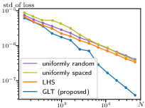
Figure 2: The number $N$ of collocation points and the standard deviation of the physics-informed loss.

Results: Accuracy of Physics-Informed Loss

First, we evaluate the accuracy of the physics-informed loss (1) in approximating the integrated loss (2). Regardless of the method, as the number $N$ of collocation points increases, the physics-informed loss (1) approaches the integrated loss (2). With fewer collocation points, the physics-informed loss varies significantly depending on the selection of collocation points, resulting in a larger standard deviation. We trained the PINNs on the NLS equation using LHS with $N=610$ collocation points. Then, we evaluated the physics-informed loss of the obtained PINNs for different methods and different numbers of collocation points. For each combination of method and number, we performed 1,000 trials and summarized their standard deviation of the physics-informed loss in Fig. 2.

Except for the GLT, the other methods exhibit a similar trend, showing a linear reduction in standard deviation on the log-log plot. This trend aligns with the theoretical result that the convergence rate of Monte Carlo methods is $O(1/\sqrt{N})$. On the other hand, the GLT demonstrates an accelerated reduction as the number $N$ increases. This result implies that by using the GLT, the physics-informed loss (1) approximates the integrated loss (2) more accurately with the same number $N$ of collocation points, leading to faster training and improved accuracy.

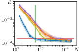
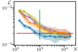
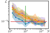
NLS	KdV	AC
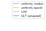
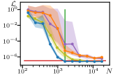
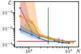
	Poisson with $s=2$	Poisson with $s=4$

Figure 3: The number $N$ of collocation points and the relative error $\mathcal{L}$.

Table 1: Trade-Off between Number $N$ of Collocation Points and Relative Error $\mathcal{L}$.

		NLS	KdV	AC	Poisson
					$s=2$	$s=4$
	$\bullet$ uniformly random	6,765	10,946	4,181	$>$17,711	1,019
# of points $N^{\dagger}$	$\bullet$ uniformly spaced	1,600	6,724	11,025	6,724	1,296
	$\bullet$ LHS	4,181	17,711	10,000	$>$17,711	562
	$\bullet$ GLT (proposed)	610	987	987	1,597	307
	$\bullet$ uniformly random	7.60	3.32	1.82	4.141	28.7
relative error $\mathcal{L}^{\ddagger}$	$\bullet$ uniformly spaced	4.88	3.25	1.79	1.859	29.2
	$\bullet$ LHS	6.45	2.94	1.43	6.174	24.3
	$\bullet$ GLT (proposed)	1.55	1.90	0.74	0.027	16.4
$\dagger$ # of points $N$ at competitive relative error $\mathcal{L}$ (under horizontal red line in Fig. 3).
$\ddagger$ relative error $\mathcal{L}$ at competitive # of points $N$ (on vertical green line in Fig. 3).
Shown in the scale of $10^{-5}$ for Poisson’s equation and $10^{-3}$ for others.

NLS ($\times 10^{2}$)	KdV ($\times 10^{2}$)

AC ($\times 10^{2}$)

Poisson with $s=2$ ($\times 10^{5}$)	Poisson with $s=4$ ($\times 10^{3}$)

Figure 4: Example results at competitive number $N$ of collocation points (on vertical green line in Fig. 3). The leftmost panel shows the true solution. The remaining panels show the residuals of PINNs’ results using uniformly random sampling, uniformly spaced sampling, LHS, and GLT, from left to right. The residuals are multiplied by the factors in parentheses.

Results: Performance of PINNs

Figure 3 shows the average relative error $\mathcal{L}$ with solid lines and the maximum and minimum errors with shaded areas. These results demonstrate that as $N$ increases, the relative error $\mathcal{L}$ decreases and eventually reaches saturation. This is because of numerical errors in the datasets, discretization errors in relative error $\mathcal{L}$, and the network capacity.

We report the minimum numbers $N$ of collocation points with which the relative error $\mathcal{L}$ was saturated in Table 1. Specifically, we consider a relative error $\mathcal{L}$ below 130 % of the minimum observed one as saturated; the thresholds are denoted by horizontal red lines in Fig. 3. The proposed GLT demonstrated equivalent performance with significantly fewer collocation points. This suggests that the proposed GLT can achieve comparable performance with significantly less computational cost. Next, we equalized the number $N$ of collocation points (and therefore, the computational cost). In the bottom rows of Table 1, we report the relative error $\mathcal{L}$ for collocation points with which the relative error $\mathcal{L}$ of one of the comparison methods saturated, as denoted by vertical green lines in Fig. 3. A smaller loss $\mathcal{L}$ indicates that the method performed better than others with the same computational cost. The proposed GLT yielded nearly half or less of the relative error $\mathcal{L}$ for the NLS, KdV, and AC equations, and the difference is significant for Poisson’s equation with $s=2$. We show the true solutions and the residuals of example results with such $N$ in Fig. 4. We also investigated longer training with smaller mini-batch sizes in Appendix C.

4.2 Competitive Physics-Informed Neural Networks

Experimental Settings

Competitive PINNs (CPINNs) are an improved version of PINNs that additionally uses a neural network $D:\Omega\rightarrow\mathbb{R}$ called a discriminator [48]. Its objective function is $\frac{1}{N}\sum_{i=1}^{N}D(\bm{x}_{i})\mathcal{N}[\tilde{u}](\bm{x}_{i})$; the discriminator $D$ is trained to maximize it, whereas the neural network $\tilde{u}$ is trained to minimize it. This setting is regarded as a zero-sum game, and its Nash equilibrium offers the solution to a given PDE. Moreover, this setting enables to use the (adaptive) competitive gradient descent (CGD) algorithm [34, 35], accelerating the convergence. The objective function is also regarded as a finite approximation to the integral $\int_{\Omega}D(\bm{x})\mathcal{N}[\tilde{u}](\bm{x})\mathrm{d}\bm{x}$; therefore, the proposed GLT can be applied to CPINNs.

We modified the code accompanying the manuscript and investigated the NLS and Burgers’ equations. The NLS equation is identical to the one above. See Appendix B for details about Burgers’ equation. The number $N$ of collocation points was 20,000 by default and varied. All experiments were conducted using Python v3.9.16 and Pytorch v1.13.1 [31] on servers with Intel Xeon Platinum 8368 and NVIDIA A100.

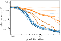
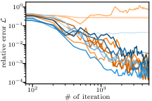
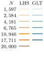
NLS	Burgers

Figure 5: The number of iterations and the relative error $\mathcal{L}$.

Results

We summarized the results in Fig. 5. For the NLS equation, when the collocation points were determined by LHS, the relative error $\mathcal{L}$ of CPINNs decreased slowly even with $N=20,000$, and there was almost no improvement for $N\leq 2,584$. On the other hand, when the proposed GLT was used, the error decreased rapidly even with $N=2,584$. In the case of the Burgers’ equation, CPINNs using GLT made some progress in learning with $N=2,584$ collocation points, while CPINNs using LHS required $N=6,765$ collocation points. These results indicate that the proposed GLT exhibits competitive or superior convergence speed with 2.5 to 8 times fewer collocation points. The original paper demonstrated that CPINNs have a faster convergence rate than vanilla PINNs, but the GLT can further accelerate it.

5 Conclusion

This paper highlighted that the physics-informed loss, commonly used in PINNs and their variants, is a finite approximation to the integrated loss. From this perspective, it proposed good lattice training (GLT) to determine collocation points. This method enables a more accurate approximation of the integrated loss with a smaller number of collocation points. Experimental results using PINNs and CPINNs demonstrated that the GLT can achieve competitive or superior performance with much fewer collocation points. These results imply a significant reduction in computational cost and contribute to the large-scale computation of PINNs.

We focused on the physics-informed loss in the domain. If the domain is $s\geq 3$-dimensional, the initial and boundary conditions are of $s\geq 2$ dimensions, and their loss functions are also subject to the proposed GLT. As shown in Figs. 3 and 5, the current problem setting reaches performance saturation with around $N=1,000$ collocation points. However, Figure 2 demonstrates that the GLT significantly enhances the approximation accuracy even when using further more collocation points. This implies that the GLT is particularly effective in addressing larger-scale problem settings, which will be explored further in future research.

Appendix

Appendix A Theoretical Background

In this section, as a theoretical background, we will provide a proof of Theorem 1, explain why the Fibonacci sequence gives a good lattice, and show how to transform a non-periodic function into a periodic one.

A.1 Proof of Theorem 1

While Theorem 1 in the main body focuses on the original physics-informed loss, in this section, we start with a general form. We aim at the objective function expressed as the form

$$\frac{1}{N}\sum_{j=1}^{N}\mathcal{P}[\tilde{u}](\bm{x}_{j}),$$ (8)

where $\mathcal{P}$ is an operator that maps a function of $\bm{x}$ to another function of $\bm{x}$. The original physics-informed loss $\frac{1}{N}\sum_{j=1}^{N}\|\mathcal{N}[\tilde{u}](\bm{x}_{j})\|^{2}$ is an example of this form, where its operator is $\mathcal{P}:\tilde{u}\mapsto\|\mathcal{N}[\tilde{u}]\|^{2}$. This form also includes the loss function $\frac{1}{N}\sum_{j=1}^{N}\|\tilde{u}(\bm{x}_{j})-g(\bm{x}_{j})\|^{2}$ for learning the Dirichlet boundary condition $u(\bm{x})=g(\bm{x})$ at $\bm{x}\in\partial\Omega$, the objective function $\frac{1}{N}\sum_{j=1}^{N}D(\bm{x}_{j})\mathcal{N}[\tilde{u}](\bm{x}_{j})$ for CPINNs [48], and those for other variants [37]. The objective function (8) can be regarded as a finite approximation to

$$\int_{[0,1]^{s}}\mathcal{P}[\tilde{u}](\bm{x})\mathrm{d}\bm{x}.$$ (9)

The main result is the following theorem.

Theorem 2.

Suppose that the activation function of $\tilde{u}$ and hence $\tilde{u}$ itself are sufficiently smooth so that there exists an $\alpha>0$ such that $\mathcal{P}[\tilde{u}]\in E_{\alpha}$. Then, for given integers $N\geq 2$ and $s\geq 2$, there exists an integer vector $\bm{z}\in\mathbb{Z}^{s}$ such that $L=\{\mbox{decimal part of\ }\frac{j}{N}\bm{z}\mid j=0,\ldots,N-1\}$ and

$$\left|\int_{[0,1]^{s}}\mathcal{P}[\tilde{u}](\bm{x})\mathrm{d}\bm{x}-\frac{1}{N}\sum_{\bm{x}_{j}\in L^{*}}\mathcal{P}[\tilde{u}](\bm{x}_{j})\right|=O\left(\frac{(\log N)^{\alpha s}}{N^{\alpha}}\right).$$

Intuitively, if $\mathcal{P}[\tilde{u}]$ satisfies certain conditions, we can find a set $L^{*}$ of collocation points with which the objective function (8) approximates the integral (9) only within an error of $O(\frac{(\log N)^{\alpha s}}{N^{\alpha}})$. This rate is much better than that of the Monte Carlo method, which is of $O(1/\sqrt{N})$ [38].

To prove Theorem 2, we introduce a theorem in the field of number theoretic numerical analysis, in which the function

$$P_{\alpha}(\bm{z},N)=\sum_{\bm{h}\in\mathbb{Z}^{s},\bm{h}\neq 0,\bm{h}\cdot\bm{z}\equiv 0\pmod{N}}\frac{1}{(\bar{h}_{1}\bar{h}_{2}\cdots\bar{h}_{s})^{\alpha}}$$

is bounded:

Theorem 3 ([38]).

For integers $N\geq 2$ and $s\geq 2$, there exists a $\bm{z}\in\mathbb{Z}^{s}$ such that

$$P_{\alpha}(\bm{z},N)\leq\frac{(2\log N)^{\alpha s}}{N^{\alpha}}+O\left(\frac{(\log N)^{\alpha s-1}}{N^{\alpha}}\right).$$

Recall that $\bar{k}=\max(1,|k|)$ for $k\in\mathbb{R}$. Suppose $\mathcal{P}[\tilde{u}]$ is sufficiently smooth and can be expanded into Fourier series using Fourier coefficients $\hat{\mathcal{P}}[\tilde{u}]$. Then, $|(\ref{eq:clossgen})-(\ref{eq:dlossgen})|$ yields

$$\left|\int_{[0,1]^{s}}\mathcal{P}[\tilde{u}](\bm{x})\mathrm{d}\bm{x}-\frac{1}{N}\sum_{j=1}^{N}\mathcal{P}[\tilde{u}](\bm{x}_{j})\right|=\left|\frac{1}{N}\sum_{j=1}^{N}\sum_{\bm{h}\in\mathbb{Z}^{s},\bm{h}\neq 0}\hat{\mathcal{P}}[\tilde{u}](\bm{h})\exp(2\pi\mathrm{i}\bm{h}\cdot\bm{x}_{j})\right|.$$

We restrict collocation points $\bm{x}_{j}$ to the form $L=\{\mbox{decimal part of\ }\frac{j}{N}\bm{z}\mid j=0,\ldots,N-1\}$ with a fixed integer vector $\bm{z}$. Following Lemma 1, we get

$$\left|\int_{[0,1]^{s}}\mathcal{P}[\tilde{u}](\bm{x})\mathrm{d}\bm{x}-\frac{1}{N}\sum_{\bm{x}_{j}\in L^{*}}\mathcal{P}[\tilde{u}](\bm{x}_{j})\right| \leq\sum_{\bm{h}\in\mathbb{Z}^{s},\bm{h}\neq 0,\bm{h}\cdot\bm{z}\equiv 0\pmod{N}}\left|\hat{\mathcal{P}}[\tilde{u}](\bm{h})\right|.$$

Because of Definition 3, if $\mathcal{P}[\tilde{u}]\in E_{\alpha}$ for some $\alpha$, there exists $c>0$ such that

$$\left|\int_{[0,1]^{s}}\mathcal{P}[\tilde{u}]\mathrm{d}\bm{x}-\frac{1}{N}\sum_{\bm{x}_{j}\in L^{*}}\mathcal{P}[\tilde{u}](\bm{x}_{j})\right|\leq\sum_{\bm{h}\in\mathbb{Z}^{s},\bm{h}\neq 0,\bm{h}\cdot\bm{z}\equiv 0\pmod{N}}\frac{c}{(\bar{h}_{1}\bar{h}_{2}\cdots\bar{h}_{s})^{\alpha}}=cP_{\alpha}(\bm{z},N).$$

Because of Theorem 3, for integers $N\geq 2$ and $s\geq 2$, there exists a $\bm{z}\in\mathbb{Z}^{s}$ such that

$$\left|\int_{[0,1]^{s}}\mathcal{P}[\tilde{u}]\mathrm{d}\bm{x}-\frac{1}{N}\sum_{\bm{x}_{j}\in L^{*}}\mathcal{P}[\tilde{u}](\bm{x}_{j})\right|\leq\frac{c(2\log N)^{\alpha s}}{N^{\alpha}}+O\left(\frac{(\log N)^{\alpha s-1}}{N^{\alpha}}\right).$$ (10)

Then, we can obtain Theorem 2.

The assumption that $\mathcal{P}[\tilde{u}]$ can be expanded using Fourier coefficients and is in the Korobov space $E_{\alpha}$ suggests that $\mathcal{P}[\tilde{u}]$ is periodic. In general, $\mathcal{P}[\tilde{u}]$ is not periodic; see Appendix A.3 for such cases.

Since $\mathcal{P}[\tilde{u}](\bm{x})=\|\mathcal{N}[\tilde{u}](\bm{x})\|^{2}$ for the original physics-informed loss is non-negative, from Theorem 2, we can say Theorem 1:

$$\int_{[0,1]^{s}}\|\mathcal{N}[\tilde{u}](\bm{x})\|^{2}\mathrm{d}\bm{x}\leq\frac{1}{N}\sum_{\bm{x_{j}}\in L^{*}}\|\mathcal{N}[\tilde{u}](\bm{x}_{j})\|^{2}+O\left(\frac{(\log N)^{\alpha s}}{N^{\alpha}}\right).$$

This implies that the minimization of the physics-informed loss (1) minimizes the integral (2) only with a small gap.

A.2 Lattice Defined by Fibonacci Sequence and Diophantine Approximation

It is known that for $s=2$, $\bm{z}\in\mathbb{Z}^{2}$ in Theorem 2 can be constructed by using the Fibonacci sequence [30, 38]. Specifically,

$$F_{1}=F_{2}=1,\quad F_{k}=F_{k-1}+F_{k-2}\ (k\geq 3),$$

$\bm{z}=(1,F_{k-1})^{\top}$ with $N=F_{k}$ satisfies the inequality in (10). It is known that $\bm{h}\cdot\bm{z}\equiv 0\pmod{N}$ gives a small $\bar{h}_{1}\bar{h}_{2}$, making $P_{\alpha}(\bm{z},N)$ large. Hence, it is preferable to choose $\bm{z}$ so that $\bm{z}$ maximizes a minimized $\bar{h}_{1}\bar{h}_{2}$:

$$\max_{\bm{z}\in\mathbb{Z}^{2}}\quad\min_{\bm{h}\in\mathbb{Z}^{2},\bm{h}\neq 0,\bm{h}\cdot\bm{z}\equiv 0\pmod{N}}\bar{h}_{1}\bar{h}_{2}.$$

Because $\{F_{k}\}$ is the Fibonacci sequence, it holds that for $\bm{h}=(F_{k-2},1)^{\top}$

$$\bm{h}\cdot\bm{z}=\begin{pmatrix}F_{k-2}\\ 1\end{pmatrix}\cdot\begin{pmatrix}1\\ F_{k-1}\end{pmatrix}=F_{k-2}+F_{k-1}=F_{k}=N\equiv 0\pmod{N}.$$

This $\bm{h}$ gives $\bar{h}_{1}\bar{h}_{2}=F_{k-2}$. It is known that this achieves a small enough $\bar{h}_{1}\bar{h}_{2}$. Since $F_{k}$ is written as

$$F_{k}=\frac{1}{\sqrt{5}}\left(\left(\frac{1+\sqrt{5}}{2}\right)^{k}-\left(\frac{1-\sqrt{5}}{2}\right)^{k}\right),$$

$F_{k}/F_{k-2}\to((1+\sqrt{5})/2)^{2}$ as $k\to\infty$. Hence, if $N=F_{k}$, then $\bar{h}_{1}\bar{h}_{2}=F_{k-2}\to N/((1+\sqrt{5})/2)^{2}$ as $k\to\infty$. Hence, roughly, $1/(\bar{h}_{1}\bar{h}_{2})^{\alpha}$ in $P_{\alpha}(\bm{z},N)$ becomes $O(1/N^{\alpha})$. See [30, 38] for more strict proof.

The following explains why the Fibonacci sequence is better from a more number-theoretic point of view. For an integer $N\geq 2$, let $\bm{z}=(1,z_{2})\in\mathbb{Z}^{2}$ with $\gcd(z_{2},N)=1$. Let the continued fraction expansion of the rational number $z_{2}/N$ be

$$\frac{z_{2}}{N}=a_{0}+1/(a_{1}+1/(a_{2}+\cdots)),$$

where $a_{0}=\lfloor\frac{z_{2}}{N}\rfloor$ and $a_{i}\in\mathbb{N}$ for $1\leq i\leq k$. Let $r_{i}$ be the rational number obtained by truncating this expansion up to $a_{i}$. It can be confirmed that $r_{i}$ can be written as $r_{i}=p_{i}/q_{i}$ using $q_{i},p_{i}\in\mathbb{Z}$, obtained as follows.

$$p_{0}=a_{0},p_{1}=a_{0}a_{1}+1,p_{i}=a_{i}p_{i-1}+p_{i-2},$$

$$q_{0}=1,q_{1}=a_{1},q_{i}=a_{i}q_{i-1}+q_{i-2}.$$

It is also confirmed that this gives the reduced form: $\gcd(p_{i},q_{i})=1$ [30].

Such a continued fraction expansion is used in the Diophantine approximation. The Diophantine approximation is one of the problems in number theory, which includes the problem of approximating irrational numbers by rational numbers. The approximations are classified into “good” approximation and “best” approximation according to the degree of the approximation, and it is known that the above continued fraction expansion gives a “good” approximation. This is why the lattice $L$ is called a “good” lattice. The accuracy of the approximation has also been studied, and it is known that in the above case, the following holds [30]:

$$\frac{1}{q_{i}(q_{i}+q_{i+1})}\leq\left|\frac{z_{2}}{N}-\frac{p_{i}}{q_{i}}\right|\leq\frac{1}{q_{i}q_{i+1}},$$

from which it follows [30] that

$$\frac{N}{\max_{1\leq i\leq k}a_{i}+2}\leq\min_{\bm{h}\in\mathbb{Z}^{2},\bm{h}\neq 0,\bm{h}\cdot\bm{z}\equiv 0\pmod{N}}\bar{h}_{1}\bar{h}_{2}\leq\frac{N}{\max_{1\leq i\leq k}a_{i}}.$$

Hence, to maximize $\min_{\bm{h}}\bar{h}_{1}\bar{h}_{2}$, it is preferable to use the pair of $z_{2}$ and $N$ such that $\max_{1\leq i\leq k}a_{i}$ is as small as possible. To this end, $a_{i}$’s should be determined by $a_{0}=0$ and $a_{i}=1$ for all $i\geq 1$. Substituting these $a_{i}$’s into the formulas for $q_{i}$ and $p_{i}$ results in

$$p_{0}=0,p_{1}=1,p_{2}=1,p_{3}=2,\ldots$$

$$q_{0}=1,q_{1}=1,q_{2}=2,q_{3}=3,\ldots$$

which means $p_{i}=F_{i-1},q_{i}=F_{i}$ where $F_{i}$’s are the Fibonacci sequence. Hence, the pair of $z_{2}=F_{k-1}$ and $N=F_{k}$ gives a “good” lattice for computing objective functions.

A.3 Periodization of Integrand

The method in this paper relies on the Fourier series expansion and hence assumes that the integrand can be periodically extended. In order to extend a given function periodically, it is convenient if the function always vanishes on the boundary. To this end, variable transformations are useful [30, 38].

For example, suppose that a function $f:[0,1]\to\mathbb{R}$ does not satisfy $f(0)=f(1)$ and the integral on an interval $[0,1]$

$$\int_{0}^{1}f(x)\mathrm{d}x$$

must be evaluated as an objective function. Let $y:[0,1]\to[0,1]$ be a monotonically increasing smooth map. Then the change of variables

$$x=y(z)\quad z\in[0,1]$$

transforms the integral into

$$\int_{0}^{1}f(x)\mathrm{d}x=\int_{0}^{1}f(y(z))\frac{\mathrm{d}y}{\mathrm{d}z}(z)\mathrm{d}z.$$

Hence, if the derivative $\mathrm{d}y/\mathrm{d}z$ vanishes at $z=0$ and $z=1$, the integrand becomes periodic. Functions that satisfy these conditions can be easily constructed using polynomials. For example, it is sufficient that this derivative is proportional to $z(1-z)$. Since $z(1-z)\geq 0$ on the interval $[0,1]$, integration of $z(1-z)$ defines a monotonically increasing smooth function, and hence this can be used to define the function $y(z)$. Smoother transformations can be designed in a similar way by using higher-order polynomials with the constraints such as $\mathrm{d}y/\mathrm{d}z=\mathrm{d}^{2}y/\mathrm{d}z^{2}=0$ at $z=0$ and $z=1$ [38].

Appendix B Datasets and Experimental Settings

In the main body, we denote the set of coordinates by $\bm{x}$. In this section, we denote each coordinate separately: the space by $x$ or $y$ and the time by $t$. We obtained the datasets of the nonlinear Schrödinger (NLS) equation, Korteweg–De Vries (KdV) equation, and Allen-Cahn (AC) equation from the official repository1 of Raissi et al., [33]. These are 2D PDEs, involving 1D space $x$ and 1D time $t$. The solutions were obtained numerically using spectral Fourier discretization and a fourth-order explicit Runge–Kutta method. In addition, we created datasets of Poisson’s equation.

Nonlinear Schrödinger Equation

A 1D NLS equation is expressed as

$$\mathrm{i}u_{t}+\gamma u_{xx}+|u|^{p-1}u=0,$$ (11)

where the coordinate is $\bm{x}=(x,t)$, the state $u$ is complex, and $\mathrm{i}$ denotes the imaginary unit. This equation is a governing equation of the wave function in quantum mechanics. The linear version, which does not have the third term, is hyperbolic. We simply treated a complex state $u$ as a 2D real vector $(w,v)$ for $u=w+\mathrm{i}v$ for training We used $\gamma=0.5$ and $p=3$, which resulted in the following equations:

$$w_{t}+0.5v_{xx}+(w^{2}+v^{2})v=0,$$ (12)

$$v_{t}-0.5w_{xx}-(w^{2}+v^{2})w=0.$$

We used the domain $\Omega=[-5,5]\times[0,\pi/2]\ni(x,t)$ and the periodic boundary condition. The initial condition was $u(x,0)=u_{0}(x)=\mathrm{sech}(x)$. For evaluation, the numerical solution $u$ at $N_{e}=256\times 201$ uniformly spaced points was provided, at which we calculated the relative error $\mathcal{L}$ of the absolute value $h=\sqrt{u^{2}+v^{2}}$. To learn the initial condition, $N_{0}=50$ collocation points $x_{1},x_{w},\dots,x_{N_{0}}$ were randomly sampled, with which the mean squared error of the state was calculated; namely $\frac{1}{N_{0}}\sum_{j=1}^{N_{0}}|\tilde{u}(x_{j},0)-u_{0}(x_{j})|^{2}_{2}$. Also for the boundary condition, $N_{b}=50$ collocation points $t_{1},t_{2},\dots,t_{N_{b}}$ were randomly sampled, with which the mean squared errors of the state and the derivative were calculated; namely $\frac{1}{N_{b}}\sum_{j=1}^{N_{b}}|\tilde{u}(-5,t_{j})-\tilde{u}(5,t_{j})|^{2}_{2}$ and $\frac{1}{N_{b}}\sum_{j=1}^{N_{b}}|\tilde{u}_{x}(-5,t_{j})-\tilde{u}_{x}(5,t_{j})|^{2}_{2}$. Then, the neural network was trained to minimize the sum of these three errors and the physics-informed loss.

Korteweg–De Vries (KdV) Equation

A 1D KdV equation is a hyperbolic PDE expressed as

$$\textstyle u_{t}+\lambda_{1}uu_{x}+\lambda_{2}u_{xxx}=0,$$ (13)

for the coordinate $\bm{x}=(x,t)$. The KdV equation is a model of shallow water waves. We used $\lambda_{1}=1$ and $\lambda_{2}=0.0025$, the domain $\Omega=[-1,1]\times[0,1]\ni(x,t)$, and the periodic boundary condition. The initial condition was $u(x,0)=u_{0}(x)=\cos(\pi x)$. For evaluation, the numerical solution $u$ at $N_{e}=512\times 201$ uniformly spaced points were provided. To guarantee the periodic boundary condition, we normalized the space $x$ as $\hat{x}=\frac{x+1}{2}\in[0,1]$ and mapped it into the unit circle as $(x_{1},x_{2})=(\cos(2\pi\hat{x}),\sin(2\pi\hat{x}))$; hence, the input to the neural network is $(x_{1},x_{2},t)$. Also, we mixed the initial condition $u_{0}(x)$ and the output $\tilde{u}(x,t)$ of the neural network as $\exp(-t)u_{0}(x)+(1-\exp(-t))\tilde{u}(x,t)$, thereby guaranteeing the initial condition. Hence, the physics-informed loss is only the objective function. This technique was introduced by Lagaris et al., [22]; it improved the final performance and, most importantly, evaluated the effect of the number $N$ of collocation points independently from the initial and boundary conditions.

Allen–Cahn Equation

A 1D AC equation is a parabolic PDE expressed as

$$\textstyle u_{t}-pu^{3}-ru-qu_{xx}=0,$$ (14)

for the coordinate $\bm{x}=(x,t)$. The AC equation describes the phase separation of co-polymer melts. We used $p=0.0001$, $r=-5$, $q=5$, the domain $\Omega=[-1,1]\times[0,1]\ni(x,t)$, and the periodic boundary condition. The initial condition was $u(x,0)=u_{0}(x)=x^{2}\cos(\pi x)$. For evaluation, the numerical solution $u$ at $N_{e}=512\times 201$ uniformly spaced points was provided. We guaranteed the initial and boundary conditions in the same manner as for the KdV equation.

Poisson’s Equation

2D Poisson’s equation is expressed as

$$\Delta u+f=0,$$ (15)

where $\Delta$ is Laplacian and $f$ is a function of coordinates, state, and its first-order derivatives. It is elliptic if the term $f$ is linear. The case of $s=2$ dimensions with the coordinate $\bm{x}=(x,y)$ is expressed as

$$u_{xx}+u_{yy}+f(x,y,u_{x},u_{y})=0.$$ (16)

For the coordinate $\bm{x}=(x^{(1)},\dots,x^{(s)})$ in general, we used the domain $\Omega=[0,1]^{s}$, the Dirichlet boundary condition $u(\bm{x})=0$ at $\partial\Omega$, and $f(\bm{x})=\prod_{i=1}^{s}\sin(k\pi x^{(i)})$. Then, we obtained the analytic solution as $u(\bm{x})=\prod_{i=1}^{s}\sin(k\pi x^{(i)})/(-sk^{2}\pi^{2})$; there are $k^{s}$ peaks or valleys. To ensure the boundary condition, we multiplied the output $\tilde{u}$ of the neural network by $\prod_{i=1}^{s}x^{(i)}(x^{(i)}-1)$. For evaluation, we obtained the analytic solution $u$ at uniformly spaced points of $N_{e}=999^{2}$ for $s=2$ and $N_{e}=49^{4}$ for $s=4$.

Table A1: Best Results when Varying Numbers of Collocation Points and Iterations

		NLS	KdV	AC
	$\bullet$ uniformly random	4.07	2.69	0.900
relative error $\mathcal{L}^{\ddagger}$	$\bullet$ uniformly spaced	2.23	3.06	0.478
	$\bullet$ LHS	3.32	2.24	0.628
	$\bullet$ GLT (proposed)	1.26	1.48	0.434

$\ddagger$ Shown in the scale of $10^{-3}$.

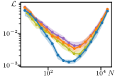
NLS	KdV	AC

Figure A1: The number $N$ of collocation points vs the relative error $\mathcal{L}$.

Burgers’ Equation

1D Burgers’ equation is expressed as

$$u_{t}+uu_{x}-\nu u_{xx}=0$$

for the coordinate $\bm{x}=(x,t)$. Burgers’ equation is a convection-diffusion equation describing a nonlinear wave. We used $\nu=(0.01/\pi)$, the domain $\Omega=[-1,1]\times[0,1]\ni(x,t)$, the Dirichlet boundary condition $u(-1,t)=t(1,t)=0$, and the initial condition $u(x,0)=u_{0}(x)=-\sin(\pi x)$. For evaluation, the numerical solution $u$ at $N_{e}=256\times 100$ uniformly spaced points was provided. From these points, we used $N_{0}=256$ and $N_{b}=100$ collocation points for learning the initial condition and boundary condition, respectively. The loss functions for these conditions were identical to those for the NLS equation.

Appendix C Additional Experiments and Results

When neural networks are trained using the SGD methods, such as Adam optimizer, and a different set of collocation points is sampled at every iteration, its number $N$ can be regarded as the mini-batch size. Neural networks might be undertrained with a small number $N$ and potentially work much better after a longer training period. To confirm this assumption, we equalized the product of the number $N$ of collocation points and the number of training iterations. Specifically, we set the number of training iterations to $200000\times 1000/N$, indicating that the training period becomes longer for $N<1000$ and shorter for $N>1000$ compared to Table 1 and Fig. 3.

We summarized the results in Table A1 and depicted them in Fig. A1. The proposed GLT outperformed comparison methods across all datasets and for a wide range of collocation points. In each iteration, PINNs are trained locally using a given set of collocation points, which may lead to forgetting training outcomes outside those regions, resulting in poor overall performance. Therefore, also in this case, it is crucial to select collocation points that cover the entire domain efficiently, and once again, the proposed GLT outperforms alternative methods.

References

- Abadi et al., [2016] Abadi, M., Agarwal, A., Barham, P., Brevdo, E., Chen, Z., Citro, C., Corrado, G. S., Davis, A., Dean, J., Devin, M., Ghemawat, S., Goodfellow, I., Harp, A., Irving, G., Isard, M., Jozefowicz, R., Jia, Y., Kaiser, L., Kudlur, M., Levenberg, J., Mané, D., Schuster, M., Monga, R., Moore, S., Murray, D., Olah, C., Shlens, J., Steiner, B., Sutskever, I., Talwar, K., Tucker, P., Vanhoucke, V., Vasudevan, V., Viégas, F., Vinyals, O., Warden, P., Wattenberg, M., Wicke, M., Yu, Y., and Zheng, X. (2016). TensorFlow: Large-scale machine learning on heterogeneous systems. USENIX Symposium on Operating Systems Design and Implementation (OSDI).
- Achdou et al., [2014] Achdou, Y., Buera, F. J., Lasry, J.-M., Lions, P.-L., and Moll, B. (2014). Partial differential equation models in macroeconomics. Philosophical Transactions of the Royal Society A: Mathematical, Physical and Engineering Sciences, 372(2028):20130397.
- Bihlo and Popovych, [2022] Bihlo, A. and Popovych, R. O. (2022). Physics-informed neural networks for the shallow-water equations on the sphere. Journal of Computational Physics, 456:111024.
- Chen et al., [2018] Chen, R. T. Q., Rubanova, Y., Bettencourt, J., and Duvenaud, D. (2018). Neural Ordinary Differential Equations. In Advances in Neural Information Processing Systems (NeurIPS), pages 1–19.
- Chen et al., [1990] Chen, S., Billings, S. A., and Grant, P. M. (1990). Non-linear system identification using neural networks. International Journal of Control, 51(6):1191–1214.
- Dissanayake and Phan-Thien, [1994] Dissanayake, M. W. M. G. and Phan-Thien, N. (1994). Neural-network-based approximations for solving partial differential equations. Communications in Numerical Methods in Engineering, 10(3):195–201.
- Fang and Wang, [1994] Fang, K.-t. and Wang, Y. (1994). Number-Theoretic Methods in Statistics. Series Title Monographs on Statistics and Applied Probability. Springer New York, NY.
- Finzi et al., [2020] Finzi, M., Stanton, S., Izmailov, P., and Wilson, A. G. (2020). Generalizing Convolutional Neural Networks for Equivariance to Lie Groups on Arbitrary Continuous Data. In International Conference on Machine Learning (ICML), pages 3146–3157.
- Furihata and Matsuo, [2010] Furihata, D. and Matsuo, T. (2010). Discrete Variational Derivative Method: A Structure-Preserving Numerical Method for Partial Differential Equations. Chapman and Hall/CRC.
- Greydanus et al., [2019] Greydanus, S., Dzamba, M., and Yosinski, J. (2019). Hamiltonian Neural Networks. In Advances in Neural Information Processing Systems (NeurIPS), pages 1–16.
- Hao et al., [2023] Hao, Z., Ying, C., Su, H., Zhu, J., Song, J., and Cheng, Z. (2023). Bi-level Physics-Informed Neural Networks for PDE Constrained Optimization using Broyden’s Hypergradients. In International Conference on Learning Representations (ICLR).
- He et al., [2016] He, K., Zhang, X., Ren, S., and Sun, J. (2016). Deep Residual Learning for Image Recognition. In IEEE Conference on Computer Vision and Pattern Recognition (CVPR), pages 1–9.
- Heldmann et al., [2023] Heldmann, F., Berkhahn, S., Ehrhardt, M., and Klamroth, K. (2023). PINN training using biobjective optimization: The trade-off between data loss and residual loss. Journal of Computational Physics, page 112211.
- Hirsch, [2006] Hirsch, C. (2006). Numerical Computation of Internal and External Flows. Butterworth-Heinemann Limited.
- Jin et al., [2021] Jin, X., Cai, S., Li, H., and Karniadakis, G. E. (2021). NSFnets (Navier-Stokes flow nets): Physics-informed neural networks for the incompressible Navier-Stokes equations. Journal of Computational Physics, 426:109951.
- Keng and Yuan, [1981] Keng, H. L. and Yuan, W. (1981). Applications of Number Theory to Numerical Analysis. Springer, Berlin, Heidelberg.
- Kingma and Ba, [2015] Kingma, D. P. and Ba, J. (2015). Adam: A Method for Stochastic Optimization. In International Conference on Learning Representations (ICLR), pages 1–15.
- Knupp and Steinberg, [2020] Knupp, P. and Steinberg, S. (2020). Fundamentals of Grid Generation. CRC Press.
- Korobov, [1959] Korobov, N. M. (1959). The approximate computation of multiple integrals. In Dokl. Akad. Nauk SSSR, volume 124, pages 1207–1210. cir.nii.ac.jp.
- Korobov, [1960] Korobov, N. M. (1960). Properties and calculation of optimal coefficients. In Dokl. Akad. Nauk SSSR, volume 132, pages 1009–1012. mathnet.ru.
- Krishnapriyan et al., [2022] Krishnapriyan, A., Gholami, A., Zhe, S., Kirby, R., and Mahoney, M. W. (2022). Characterizing possible failure modes in physics-informed neural networks. In Advances in Neural Information Processing Systems (NeurIPS), pages 1–13.
- Lagaris et al., [1998] Lagaris, I. E., Likas, A., and Fotiadis, D. I. (1998). Artificial neural networks for solving ordinary and partial differential equations. IEEE Transactions on Neural Networks, 9(5):987–1000.
- Logan, [2015] Logan, J. D. (2015). Applied Partial Differential Equations. Undergraduate Texts in Mathematics. Springer Cham, Cham.
- Loshchilov and Hutter, [2017] Loshchilov, I. and Hutter, F. (2017). SGDR: Stochastic gradient descent with warm restarts. In International Conference on Learning Representations (ICLR), pages 1–16.
- Lu et al., [2019] Lu, L., Jin, P., and Karniadakis, G. E. (2019). DeepONet: Learning nonlinear operators for identifying differential equations based on the universal approximation theorem of operators. arXiv, 3(3):218–229.
- Lu et al., [2022] Lu, Y., Blanchet, J., and Ying, L. (2022). Sobolev Acceleration and Statistical Optimality for Learning Elliptic Equations via Gradient Descent. In Advances in Neural Information Processing Systems (NeurIPS).
- Mao et al., [2020] Mao, Z., Jagtap, A. D., and Karniadakis, G. E. (2020). Physics-informed neural networks for high-speed flows. Computer Methods in Applied Mechanics and Engineering, 360:112789.
- Matsubara and Yaguchi, [2023] Matsubara, T. and Yaguchi, T. (2023). FINDE: Neural Differential Equations for Finding and Preserving Invariant Quantities. In International Conference on Learning Representations (ICLR).
- Morton and Mayers, [2005] Morton, K. W. and Mayers, D. F. (2005). Numerical Solution of Partial Differential Equations: An Introduction. Cambridge University Press, Cambridge, second edition.
- Niederreiter, [1992] Niederreiter, H. (1992). Random Number Generation and Quasi-Monte Carlo Methods. CBMS-NSF Regional Conference Series in Applied Mathematics. Society for Industrial and Applied Mathematics.
- Paszke et al., [2017] Paszke, A., Chanan, G., Lin, Z., Gross, S., Yang, E., Antiga, L., and Devito, Z. (2017). Automatic differentiation in PyTorch. In NeurIPS2017 Workshop on Autodiff, pages 1–4.
- Pokkunuru et al., [2023] Pokkunuru, A., Rooshenas, P., Strauss, T., Abhishek, A., and Khan, T. (2023). Improved Training of Physics-Informed Neural Networks Using Energy-Based Priors: A Study on Electrical Impedance Tomography. In International Conference on Learning Representations (ICLR).
- Raissi et al., [2019] Raissi, M., Perdikaris, P., and Karniadakis, G. E. (2019). Physics-informed neural networks: A deep learning framework for solving forward and inverse problems involving nonlinear partial differential equations. Journal of Computational Physics, 378:686–707.
- Schaefer and Anandkumar, [2019] Schaefer, F. and Anandkumar, A. (2019). Competitive Gradient Descent. In Advances in Neural Information Processing Systems (NeurIPS), pages 1–11.
- Schaefer et al., [2020] Schaefer, F., Zheng, H., and Anandkumar, A. (2020). Implicit competitive regularization in GANs. In International Conference on Machine Learning (ICML), pages 8533–8544. PMLR.
- Shankar et al., [2018] Shankar, V., Kirby, R. M., and Fogelson, A. L. (2018). Robust Node Generation for Mesh-free Discretizations on Irregular Domains and Surfaces. SIAM Journal on Scientific Computing, 40(4):A2584–A2608.
- Sharma and Shankar, [2022] Sharma, R. and Shankar, V. (2022). Accelerated Training of Physics-Informed Neural Networks (PINNs) using Meshless Discretizations. In Advances in Neural Information Processing Systems.
- Sloan and Joe, [1994] Sloan, I. H. and Joe, S. (1994). Lattice Methods for Multiple Integration. Clarendon Press.
- Thomas, [1995] Thomas, J. W. (1995). Numerical Partial Differential Equations: Finite Difference Methods, volume 22 of Texts in Applied Mathematics. Springer, New York, NY.
- Thompson et al., [1985] Thompson, J. F., Warsi, Z. U. A., and Mastin, C. W. (1985). Numerical grid generation: foundations and applications. Elsevier North-Holland, Inc., USA.
- Vaswani et al., [2017] Vaswani, A., Shazeer, N., Parmar, N., Uszkoreit, J., Jones, L., Gomez, A. N., Kaiser, Ł., and Polosukhin, I. (2017). Attention is all you need. In Advances in Neural Information Processing Systems (NeurIPS).
- [42] Wang, C., Li, S., He, D., and Wang, L. (2022a). Is $L2̂$ Physics Informed Loss Always Suitable for Training Physics Informed Neural Network? In Advances in Neural Information Processing Systems (NeurIPS).
- Wang and Perdikaris, [2023] Wang, S. and Perdikaris, P. (2023). Long-time integration of parametric evolution equations with physics-informed DeepONets. Journal of Computational Physics, 475:111855.
- Wang et al., [2021] Wang, S., Teng, Y., and Perdikaris, P. (2021). Understanding and Mitigating Gradient Flow Pathologies in Physics-Informed Neural Networks. SIAM Journal on Scientific Computing, 43(5):A3055–A3081.
- [45] Wang, S., Yu, X., and Perdikaris, P. (2022b). When and why PINNs fail to train: A neural tangent kernel perspective. Journal of Computational Physics, 449:110768.
- Wang and Lin, [1998] Wang, Y. J. and Lin, C. T. (1998). Runge-Kutta neural network for identification of dynamical systems in high accuracy. IEEE Transactions on Neural Networks, 9(2):294–307.
- Zaremba, [2014] Zaremba, S. K. (2014). Applications of Number Theory to Numerical Analysis. Academic Press.
- Zeng et al., [2023] Zeng, Q., Kothari, Y., Bryngelson, S. H., and Schaefer, F. T. (2023). Competitive Physics Informed Networks. In International Conference on Learning Representations (ICLR), pages 1–12.