Predicting Coupled Electron and Phonon Transport Using Steepest-Entropy-Ascent Quantum Thermodynamics

Abstract

The current state of the art for determining thermoelectric properties is limited to the investigation of electrons or phonons without including the inherent electron-phonon coupling that is in all materials. This gives rise to limitations in accurately calculating base material properties that are in good agreement with experimental data. Steepest-entropy-ascent quantum thermodynamics is a general non-equilibrium quantum thermodynamic ensemble framework that provides a general equation of motion for non-equilibrium system state evolution. This framework utilizes the electron and phonon density of states as input to compute material properties, while taking into account the electron-phonon coupling. It is able to span across multiple spatial and temporal scales in a single analysis. Any system’s thermoelectric properties can, therefore, be attained provided the accurately determined density of states is available.

Keywords

quantum thermodynamics; steepest entropy ascent; computational physics; thermoelectric materials

Program Summary

Manuscript Title: Predicting Coupled Electron and Phonon Transport Using Steepest-Entropy-Ascent Quatnum Thermodynamics

Authors: Jarod Worden, Michael von Spakovsky, Celine Hin

Program Title: SEAQT

Journal Reference:

Catalogue Identifier:

Licensing Provisions: Contact Michael von Spakovsky (vonspako@vt.edu) or Celine Hin (celhin@vt.edu); the code is under copyright and will require a free license for the academic and national lab communities and a commercial license for industry.

Programming Language: MATLAB and Python

Computer: The program needs a MATLAB version $\geq$ MATLAB 2020b and a python version $\geq 3.6$

Operating System: Unix/Linux

RAM: The amount of RAM follows similar specifications as MATLAB, with 3695 MB used for the systems being analyzed in this paper.

Run Time: 5 minutes for the system parameters discussed in the paper.

Github URL: Contact Michael von Spakovsky (vonspako@vt.edu) or Celine Hin (celhin@vt.edu)

1 Introduction

Non-equilibrium phenomena are notoriously difficult to model particularly when a material system is complex (e.g., involves internal structures such as point and line defects, interfaces, etc.) and the phenomena coupled. Yet these systems are typically the ones of greatest interest. Many methods for describing these phenomena at levels ranging from the microscopic to the mesoscopic to the continuum level have been developed and include non-equilibrium molecular dynamics (NEMD), Monte Carlo (MC) methods, continuum models, etc. All of these methods, however, are limited in their spatial and temporal applicability due to computational overheads (see Fig. 1) and are characterized by a number of other limitations [1, 2, 3, 4, 5, 6, 7]. For example, a limitation of NEMD is that to determine intensive properties such as temperature and pressure, it must assume local equilibrium conditions since it is unable to predict non-quasiequilibrium processes producing non-local equilibrium states [8]. The non-equilibrium Green’s function method is a rigorous and general framework for modeling non-equilibrium processes but requires a large number of approximations of the momentum, charge, and energy conservation laws from a many-body standpoint that can fail badly even with plausible approximations [7]. Kinetic MC uses transition rates to model stochastic trajectories that propagate in a system from state to state but requires high accuracy for the pre-defined, possibly incomplete list, of possible kinetic processes, leading to incorrect or limited results [9]. The Boltzmann transport equations predict the evolution of individual energy levels through scattering processes based on Newton’s laws or quantum mechanics but are limited based on the local equilibrium requirement [10]. Continuum models with non-equilibrium effects follow a two-step process of first approximating the non-equilibrium system, using a fine mesh of local systems, each of which is assumed to be in equilibrium, and then addressing the non-equilibrium effects of system dynamics via the inclusion of a set of phenomenological coefficients (diffusivity, conductivities, etc.). Both steps represent incomplete and inadequate descriptions where the mesh is limited in its ability to describe each actual local state and the coefficients are often based on uncoupled behavior. Other limitations come from linearizations that constrain system behavior that, in fact, is nonlinear in character. A further limitation is that all of these models must evaluate a material’s characteristics at equilibrium even though it is the characteristics at non-equilibrium which are of interest [11].

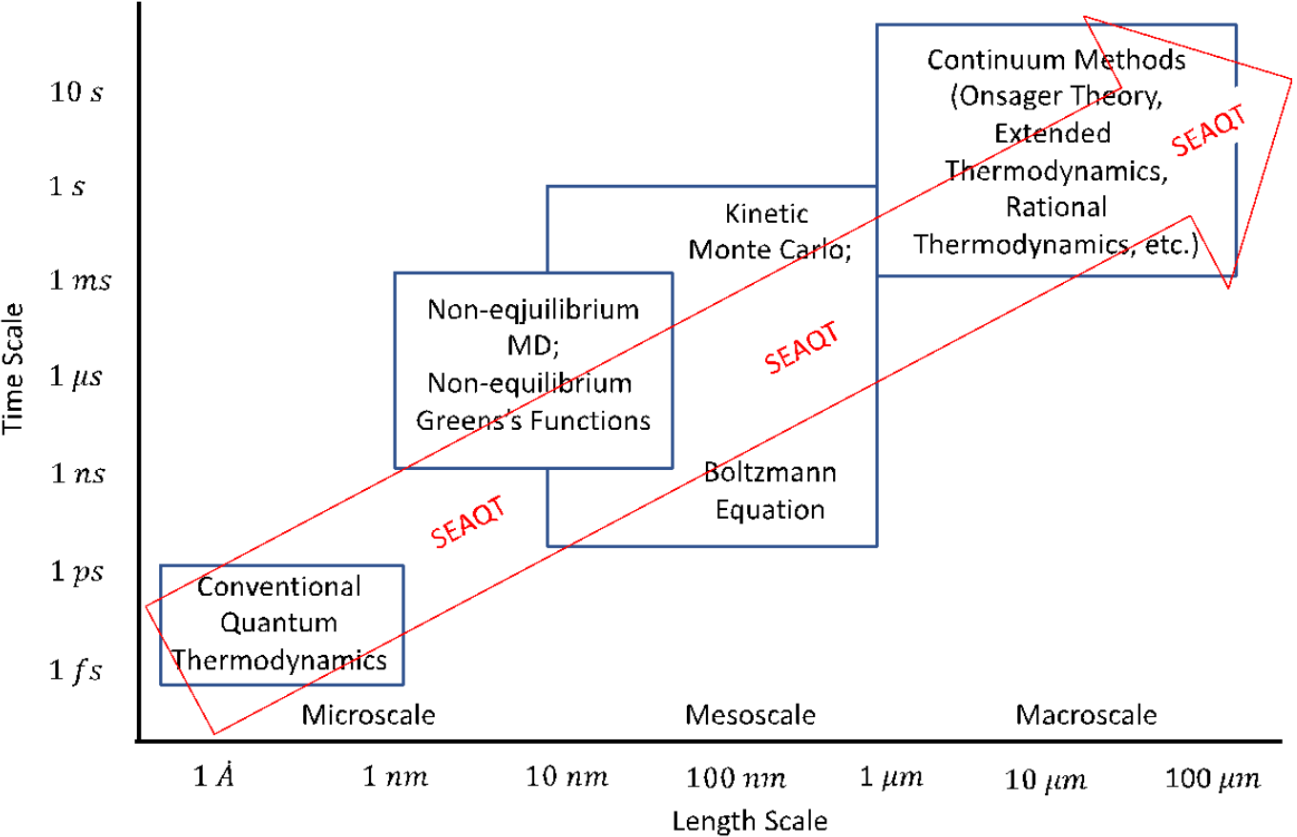
Figure 1: Plot showing the length and time scale applicability of the various methods.

In order to go beyond the limitations of these methods, a general non-equilibrium quantum thermodynamic ensemble-based framework called steepest-entropy-ascent quantum thermodynamics (SEAQT) can be used. It provides a general thermodynamically rigorous equation of motion for non-equilibrium system state evolution. This method is able to predict the non-equilibrium evolution in system state based on the principle of steepest entropy ascent (SEA) consistent with the second law of thermodynamics and satisfying all relevant conservation laws and postulates of quantum mechanics [12, 13, 14, 15]. Utilizing the hypoequilibrium concept and the density of state method developed by Li and von Spakovsky [15, 16, 17, 18, 19], the SEAQT framework can be applied from a practical standpoint at all temporal and spatial scales as illustrated in Fig. 1. The SEAQT equation of motion can be used to investigate the evolution of local non-equilibrium states from an entropy generation standpoint. Use of the hypoequilibrium concept extends the thermodynamic equilibrium description of intensive properties (e.g., temperature, pressure, and chemical potential), the Gibbs relation, etc. to the non-equilibrium realm and with the SEA principle generalizes the Onsager relations to the entire non-equilibrium realm based on thermodynamic principles only. The SEAQT equation of motion i) is applicable throughout the non-equilibrium realm, ii) is able to easily model coupled phenomena, iii) can model complex material structures involving defects and interfaces, iv) is able to cross multiple spatial and temporal scales in a single analysis, v) is applicable to quantum and classical systems, and vi) has a significantly reduced computational burden when compared to conventional approaches. The framework can, thus, be used to effectively predict the transport properties of thermoelectric materials such as the electrical conductivity, thermal conductivity, Seebeck coefficient, $ZT$ factor, etc. in time and with temperature.

The SEAQT equation of motion along with the electron and phonon density of states (DOS) of a number of different materials are utilized here to determine the values in time of critical material thermoelectric properties. These values are then compared with experimental and computational benchmark data. Many methods have been developed for interpolating the electron DOS to obtain electron transport properties. The current benchmark for such calculations is the BoltzTraP code that utilizes smooth Fourier interpolation of the band energies, while maintaining group symmetries [20]. Other electron transport calculation methods include Boltzwann [21] and LanTraP [22], which use a maximally-localized Wannier function basis and the Landauer formalism of transport theory, respectively. A primary limitation of these methods is the exclusion of the coupling aspect of the electron-phonon interactions that are present in all materials, but are especially important in metals and heavily doped materials. Other limitations include the inability of calculating the total thermal conductivity, the assumption of a constant relaxation time, and the inability to analyze polycrystalline materials and materials with defects. Many codes such as LAMMPS [23] and phonopy [24] are useful in determining strictly phonon transport properties but suffer similar limitations such as the lack of electron-phonon coupling so that only the lattice thermal conductivity and not the total thermal conductivity is calculated. All the calculations come with a large computational burden.

2 SEAQT Framework

2.1 SEAQT equation of motion

The development present here is based on that given in [11, 14, 15, 16, 18]. The equation of motion of the SEAQT framework moves through thermodynamic state space (e.g., Hilbert space) where there are m single particle energy eigenlevels that can be occupied by particles. A system eigenstate is denoted by |$n^{a}n^{b}\ldots n^{m}$⟩ where $n^{k}$ is the occupation number and $\epsilon^{k}$ the energy of the k^th single-particle energy eigenlevel. For fermions, $n^{k}$ has a value of 0 or 1, and for bosons, a value between 0 and $\infty$. A system thermodynamic state is selected from the Hilbert space spanned by the system eigenstates and can be represented by a w-dimensional vector {$p_{n^{k}}^{k}$} where $p_{n^{k}}^{k}$ represents the probability that $n^{k}$ particles are observed at the emphk^th single-particle energy eigenlevel. The system thermodynamic state can alternatively be denoted by $\gamma$, which is the square root of the probability vector given by

$$\gamma=\textrm{vect}(\gamma_{n^{k}}^{k})=\textrm{vect}(\sqrt{p_{n^{k}}^{k}}),k=a,\ldots{},m$$ (1)

$\gamma$-space is then defined as a manifold $\mathscr{L}$ whose elements are all of the w vectors of the real finite numbers X = vect($x_{l}$) and Y = vect($y_{l}$) with an inner product expressed as

$$(X|Y)=\sum_{l=1}^{w}x_{l}y_{l}$$ (2)

The time evolution of the thermodynamic state $\gamma(t)$ follows the equation of motion, which in $w$-vector form is written as

$$|d\gamma/dt)=|\Pi_{\gamma})$$ (3)

|$\Pi_{\gamma}$) is an element of the manifold $\mathscr{L}$ used to describe the local production densities associated with the balance equations for the entropy and the conserved quantities and is derived from the SEA principle subject to a set of conservation laws denoted by {$\tilde{C}(\gamma)$}. In this particular development, these include the conservation of energy, $\tilde{H}(\gamma)=\sum_{k}\sum_{n}n^{k}\epsilon_{k}p_{n^{k}}^{k}$, and of particle number, $\tilde{N}(\gamma)=\sum_{k}\sum_{n}n^{k}p_{n^{k}}^{k}$, as well as $m\$probability normalization conditions ${\tilde{I}}_{k}(\gamma)$. Using Eq. (2), the time evolution of these conserved system properties {$\tilde{C}(\gamma)$} = {$\tilde{H}$,$\tilde{N}$,${\tilde{I}}_{a}$,…,${\tilde{I}}_{m}$} and the system entropy $\tilde{S}(\gamma)$ must satisfy to the following set of equations:

$$\Pi_{C_{i}}\equiv dC_{i}/dt=(\Psi_{i}|\Pi_{\gamma})=0,\;\;\textrm{with }|\Psi_{i})\equiv|\delta{\tilde{C}}_{i}(\gamma)/\delta\gamma)$$ (4)

$$\Pi_{S}\equiv dS/dt=(\Phi|\Pi_{\gamma})\geq 0,\;\;\textrm{with }|\Phi)\equiv|\delta\tilde{S}(\gamma)/\delta\gamma)$$ (5)

where $|\Psi_{i})$ and $|\Phi)$ are functional derivatives of the system properties defined by Eqs. (A1) to (A4) of $Appendix\;A$ of Li, von Spakovaky, and Hin [11].

The time evolution of system state is a trajectory in thermodynamic state space that obeys the SEA principle. This corresponds to a variational problem that finds the instantaneous “direction” of |$\Pi_{\gamma}$) at each instant of time that maximizes the rate of entropy production $\Pi_{S}$ consistent with the conservation constraints $\Pi_{C_{i}}=0$. This requires the state space to have a metric field with which to determine the norm of $\Pi_{\gamma}$ and the distance traveled during the evolution of state. The differential of this distance is then expressed as

$$dl=\sqrt{(\Pi_{\gamma}|\hat{G}(\gamma)|\Pi_{\gamma})}dt$$ (6)

Here, $\hat{G}(\gamma)$ is a real, symmetric, positive-definite operator on the manifold, which defines the thermodynamic state space [11, 14]. It is chosen here to be the identity operator, which corresponds to the Fisher-Rao metric. The SEA variational problem then consists of maximizing $\Pi_{S}$ subject to the conservation constraints $\Pi_{C_{i}}=0$ and the additional constraint ($dl$/$dt$)² $=\varepsilon$, which ensures that the norm of $\Pi_{\gamma}$ remains constant. Here, $\varepsilon$ is a small constant. To find the solution, the method of Lagrange multipliers is used such that

$$\Upsilon=\Pi_{S}-\sum_{i}\beta_{i}\Pi_{C_{i}}-\frac{\tau}{2}(\Pi_{\gamma}|\hat{G}(\gamma)|\Pi_{(\gamma)})$$ (7)

where $\beta_{i}$ and $\tau$/2 are the Lagrange multipliers. The variational derivative of $\Upsilon$ with respect to |$\Pi_{\gamma}$) is now set equal to zero so that

$$\frac{\delta\Upsilon}{\delta\Pi_{\gamma}}=|\Phi)-\sum_{i}\beta_{i}|\Psi_{i})-\tau\hat{G}|\Pi_{\gamma})=0\$$ (8)

Solving this last equation for $|\Pi_{(\gamma)})$ yields the SEA equation of motion, i.e.,

$$|\Pi_{\gamma})=\hat{L}|\Phi)-\hat{L}\sum_{i}\beta_{i}|\Psi_{i})$$ (9)

In this last expression, $\hat{L}\equiv{\hat{G}}^{-1}$/$\tau\$ is assumed to be a diagonal operator. The diagonal terms of $\hat{L}\ \{\tau_{n^{k}}^{k},\,k=1,\ldots,m;\,n^{k}=0,1$ for fermions and $0,1,\ldots,\infty$ for bosons$\}$ are associated with the relaxation parameters of the system single–particle eigenlevels such that

$$\hat{L}=\textrm{diag}\Bigl{\{}\frac{1}{\tau_{n^{k}}^{k}}\Bigl{\}}$$ (10)

The values of the Lagrange multipliers are determined by substituting Eq. (9) into Eqs. (4) and (5) yielding

$$\sum_{j=1}^{m+2}(\Psi_{i}|\hat{L}|\Psi_{j})\beta_{j}=(\Psi_{i}|\hat{L}|\Phi)$$ (11)

where the $\beta_{j}$ are proportional to the measurements of non-equilibrium system intensive properties such as the temperature, pressure, and chemical potential [18].

Now, substituting the functional derivatives of the system properties as defined in $Appendix\;A$ of Li, von Spakovaky, and Hin [11], the equations of motion for the $\gamma^{k}$ and the $p_{n}^{k}$, of the single-particle eigenlevel probability distributions are expressed as

$$\frac{d\gamma_{n^{k}}^{k}}{dt}=\frac{1}{\tau_{n^{k}}^{k}}(-\gamma_{n^{k}}^{k}ln(p_{n^{k}}^{k})-n^{k}\epsilon^{k}\gamma_{n^{k}}^{k}\beta_{E}-n^{k}\gamma_{n^{k}}^{k}\beta_{N}-\gamma_{n^{k}}^{k}\beta_{l}^{k})$$ (12)

$$\frac{dp_{n^{k}}^{k}}{dt}=\frac{1}{\tau_{n^{k}}^{k}}(-p_{n^{k}}^{k}ln(p_{n^{k}}^{k})-n^{k}\epsilon^{k}p_{n^{k}}^{k}\beta_{E}-n^{k}p_{n^{k}}^{k}\beta_{N}-p_{n^{k}}^{k}\beta_{l}^{k})$$ (13)

where $\beta_{E}$, $\beta_{N}$, and $\beta_{l}^{k}$ are the Lagrange multipliers corresponding, respectively, to the generators of the motion $\hat{H}$, $\hat{N}$, and ${\hat{I}}_{k}$.

2.2 Hypoequilibrium concept

In [15, 16, 18], Li and von Spakovsky introduce the hypoequilibrium concept to simplify the presentation of the equation of motion and facilitate physically interpreting the state evolution. Without significant loss in generality, the assumption is made that the particles in the same single-particle energy ($\epsilon$) eigenlevel initially are in mutual stable equilibrium relative to the temperature $T^{\epsilon}$ and the chemical potential $\mu^{\epsilon}$. As a result, the initial probability distribution $p_{n^{\epsilon}}^{\epsilon}$ of the occupation states is Maxwellian, i.e.,

$$p_{n^{\epsilon}}^{\epsilon}=e^{-\beta_{l}^{\epsilon}-\beta_{N}^{\epsilon}-\beta_{E}^{\epsilon}n^{\epsilon}\epsilon}$$ (14)

where $\beta_{E}^{\epsilon}\equiv\,\frac{1}{k_{B}T^{\epsilon}}$, $\beta_{N}^{\epsilon}\equiv\,\frac{\mu^{\epsilon}}{k_{B}T^{\epsilon}}$, $k_{B}$ is Boltzmann’s constant, and $\beta_{l}^{\epsilon}\,\equiv\,\ln\,\Xi^{\epsilon}$ with the single-particle level partition function, $\Xi^{\epsilon}$, expressed as

$$\Xi^{\epsilon}(\beta_{E}^{\epsilon},\beta_{N}^{\epsilon})=\sum_{n^{\epsilon}}^{\infty}e^{-\beta_{N}^{\epsilon}n^{k}}e^{-\beta_{E}^{\epsilon}n^{\epsilon}\epsilon}$$ (15)

Such an initial state is an $m^{th}$-order hypoequilibirum state where $m$ is the total number of eigenlevels. It is a representation of the initial non-equilibrium state. An additional assumption made is that the different occupation states of the same single-particle eigenlevel have the same relaxation parameter so that

$$\tau_{n^{\epsilon}}^{\epsilon}=\tau^{e}\textrm{ for all }n^{\epsilon}\textrm{with the same }\epsilon$$ (16)

This makes each relaxation parameter a property of a particular single-particle eigenlevel. As is proven in [15], with these two assumptions, the equation of motion, Eq. (13), maintains the state of the system in a hypoequilibrium state throughout the entire time evolution. As a result, the evolution of state can be found from the motion of the state of a single-particle eigenlevel such that

$$y^{\epsilon}=\beta_{N}^{\epsilon}+\beta_{E}^{\epsilon}\epsilon$$ (17)

The equation of motion for $y^{\epsilon}$ is then found by substituting Eq. (14) into (13) resulting in

$$\frac{dy^{\epsilon}}{dt}=-\frac{1}{\tau^{\epsilon}}(y^{e}-\beta_{E}\epsilon-\beta_{N})$$ (18)

Now, multiplying Eq. (13) by the extensive value of the particle number, $\langle N\rangle_{\epsilon}$, and integrating over $n^{\epsilon}$ and doing likewise with the extensive values for the energy, $\langle e\rangle_{\epsilon}$, and the entropy, $\langle s\rangle_{\epsilon}$, the following equations result that capture the contributions to these properties from a single-particle energy eigenlevel, i.e.,

$$\frac{d{\langle N\rangle}_{\epsilon}}{dt}=\frac{1}{\tau^{\epsilon}}A_{NN}^{\epsilon}(y^{\epsilon}-\beta_{E}\epsilon-\beta_{N})$$ (19)

$$\frac{d{\langle e\rangle}_{\epsilon}}{dt}=\epsilon\frac{d{\langle N\rangle}_{\epsilon}}{dt}$$ (20)

$$\frac{d{\langle s\rangle}_{\epsilon}}{dt}=y^{\epsilon}\frac{d{\langle N\rangle}_{\epsilon}}{dt}$$ (21)

where $A_{NN}^{\epsilon}$, which is the particle number fluctuation of the single-particle energy eigenlevel, given by

$$A_{NN}^{\epsilon}={\langle N^{2}\rangle}^{\epsilon}-({\langle N\rangle}^{\epsilon})^{2}=\frac{\partial^{2}}{\partial\beta_{N}^{\epsilon}}\textrm{ln}\Xi^{\epsilon}=-\frac{\partial{\langle N\rangle}^{\epsilon}}{\partial\beta_{N}^{\epsilon}}=\frac{1}{e^{y}\pm 1}\,\mp\,\frac{1}{(e^{y}\pm 1)^{2}}$$ (22)

Here, fermions are represented with the plus sign and bosons with the negative.

2.3 Electron transport equation

For the transport of electrons between two locations (systems) $A$ and $B$, the single-particle energy eigenlevels involved are those of $A$, $\{\epsilon^{A,k}\}$, and $B$, $\{\epsilon^{B,l}\}$. Integrating Eq. (19) over the eigenlevels at location A results in

$$\frac{d{\langle N\rangle}^{A}}{dt}=\int\frac{V}{\tau^{A,\epsilon}}A_{NN}^{A,\epsilon}(\beta_{E}^{A,\epsilon}\epsilon+\beta_{N}^{A,\epsilon}-\beta_{E}\epsilon-\beta_{N})D^{A}(\epsilon)d\epsilon$$ (23)

In this last expression, $V$ is the volume of system $A$ and $D^{A}(\epsilon)$ the DOS per unit volume of $A\$. In the near-equilibrium region, both systems $A\$ and $B\$ are approximately in stable equilibrium and as a result, $\beta_{N}^{A,\epsilon}=\beta_{N}^{A}$ and $\beta_{E}^{A,\epsilon}=\beta_{E}^{A}$, so that Eq. (23) can be rewritten as

$$\frac{d{\langle N\rangle}^{A}}{dt}=(\beta_{N}^{A}-\beta_{N})\int\frac{V}{\tau^{A,\epsilon}}A_{NN}^{A,\epsilon}D^{A}(\epsilon)d\epsilon\,+(\beta_{E}^{A}-\beta_{E})\int\frac{V\epsilon}{\tau^{A,\epsilon}}A_{NN}^{A,\epsilon}D^{A}(\epsilon)d\epsilon$$ (24)

A similar development holds for $\frac{d{\langle N\rangle}^{B}}{dt}$.

This near-equilibrium assumption allows use of the zeroth-order approximation of the terms inside the integrals, leaving only the first-order approximation of $d{\langle N\rangle}^{A}$/$dt\$. Thus, it is assumed that $A\$and $B\$have the same energy eigenstructure and DOS so that

$$\tau^{A,\epsilon}=\tau^{B,\epsilon}=\tau^{\epsilon}$$ (25)

and

$$D^{A}(\epsilon)=D^{B}(\epsilon)=D(\epsilon)$$ (26)

and that the fluctuations of systems $A\$and $B\$are approximately equal to their mutual equilibrium value at $\left(\beta_{N},\beta_{E}\right)$, i.e.,

$$A_{NN}^{A,\epsilon}=A_{NN}^{B,\epsilon}=A_{NN}^{\epsilon}\left(\beta_{N},\beta_{E}\right)$$ (27)

Now, using these last three conditions and particle conservation, the flow from $B\$to $A\$is given by

$$\frac{d{\langle N\rangle}^{A}}{dt}-\frac{d{\langle N\rangle}^{B}}{dt}=2\frac{d{\langle N\rangle}^{A}}{dt}=(\beta_{N}^{A}-\beta_{N}^{B})\int\frac{V}{\tau^{\epsilon}}A_{NN}^{\epsilon}D(\epsilon)d\epsilon+(\beta_{E}^{A}-\beta_{E}^{B})\int\frac{V\epsilon}{\tau^{\epsilon}}A_{NN}^{\epsilon}D(\epsilon)d\epsilon$$ (28)

Furthermore, defining $\delta[\beta_{E}(\epsilon+\mu)]\equiv(\beta_{N}^{A}+\epsilon\beta_{E}^{A})-(\beta_{N}^{B}+\epsilon\beta_{E}^{B})$ where $\mu\equiv\beta_{N}/\beta_{E}$, the total particle flux to $A\$, $J_{N}$, can be written as

$$J_{N}\equiv\frac{2}{A_{c}}\frac{d{\langle N\rangle}^{A}}{dt}=\frac{1}{A_{c}}\int\delta[\beta_{E}(\epsilon+\mu)]\frac{V}{\tau^{\epsilon}}A_{NN}^{\epsilon}D(\epsilon)d\epsilon$$ (29)

where $A_{c}$ is the interface cross-sectional area between systems $A$ and $B$. Introducing the following variational relation for every energy eigenlevel

$$\delta[\beta_{E}(\epsilon+\mu)]=\left((\epsilon+\mu)\frac{d\beta_{E}}{dx}+\beta_{E}\frac{d\mu}{dx}\right)\delta x$$ (30)

where $\delta x\$is the distance between locations $A\$and $B$, the total flux can be reformulated as

$$J_{N}=\frac{\delta x}{A_{c}}\int\frac{V}{\tau^{\epsilon}}\left((\epsilon+\mu)\frac{d\beta_{E}}{dx}+\beta_{E}\frac{d\mu}{dx}\right)A_{NN}^{\epsilon}D(\epsilon)d\epsilon$$ (31)

If initially the system is in a hypoequilibrium state, the fluctuation $A_{NN}^{\epsilon}$ can be related to the Fermi distribution $f$ by

$$A_{NN}^{\epsilon}=\beta_{E}^{-1}\frac{\partial f}{\partial\epsilon},\;\;\textrm{ with }f=\frac{1}{e^{\beta_{E}\epsilon+\beta_{N}}+1}$$ (32)

and as a result, the particle flux becomes

$$J_{N} =-\frac{V\delta x}{A_{c}}\left(\frac{dE_{f}^{0}}{dx}+e\mathcal{E}\right)\int\frac{1}{\tau^{\epsilon}}\frac{\partial f}{\partial\epsilon}D(\epsilon)d\epsilon$$

$$\;\;\;\;\>+\frac{V\delta x}{A_{c}}\beta_{E}^{-1}\frac{d\beta_{E}}{dx}\int\frac{1}{\tau^{\epsilon}}\left(\epsilon-E_{f}\right)\frac{\partial f}{\partial\epsilon}D(\epsilon)d\epsilon$$ (33)

where $E_{f}=E_{f}^{0}+e\Phi=-\mu=-\beta_{N}/\beta_{E}$, $e$ is the electric charge, $\Phi$ the electric field potential, $E_{f}^{0}$ the fermi level without an external field, $-d\mu=dE_{f}^{0}+ed\Phi$ the differential chemical potential, and $d\Phi/dx=\mathcal{E}$ the external field.

As shown in Li, von Spakovsky, and Hin [11], Eq. (33), which results from the SEAQT equation of motion, recovers the Boltzmann transport equation (BTE) [25] in the low-field region even though the former operates in state space, while the latter does so in phase space. As a result, the SEAQT and BTE relaxation parameters $\tau^{\epsilon}$ and $\tau^{\prime}$, respectively, can be related via the following relation:

$$\tau^{\epsilon}=\frac{\left(\delta x/v_{x}\right)^{2}}{\tau^{\prime}(\epsilon)}=\frac{3m(\delta x)^{2}}{2\epsilon\tau^{\prime}(\epsilon)}$$ (34)

Here, m is the particle mass and $v_{x}$ a group or particle velocity.

2.4 Phonon transport equation

The derivation of the SEAQT equation for phonon transport is similar to that for electron transport except that there is no particle number conservation. Thus, the conservation laws only involve the energy and the probabilities such that $\{\tilde{C}(\gamma)\}=\{\tilde{H},\tilde{I}_{a},\ldots,\tilde{I}_{m}\}$. As was the case for the electrons, the hypoequilibirum concept is used for the initial states so that the time evolution of the energy at location (system) $A\$is given by

$$\frac{d{\langle E\rangle}^{A}}{dt}=\int\frac{V}{\tau^{A,\epsilon}}\epsilon^{2}A_{NN}^{A,\epsilon}\left(\beta_{E}^{A,\epsilon}-\beta_{E}\right)D^{A}(\epsilon)d\epsilon$$ (35)

Again, as before, in the near-equilibrium region, $\beta_{N}^{A,\epsilon}=\beta_{N}^{A}$ and $\beta_{E}^{A,\epsilon}=\beta_{E}^{A}$ and Eqs. (25) to (27) hold so that the energy flow from $B\$to $A\$is written as

$$\frac{d{\langle E\rangle}^{A}}{dt}-\frac{d{\langle E\rangle}^{B}}{dt}=\frac{V}{A_{c}}\left(\beta_{E}^{A}-\beta_{E}^{B}\right)\int\frac{\epsilon^{2}}{\tau^{\epsilon}}A_{NN}^{\epsilon}D(\epsilon)d\epsilon=\frac{V\delta x}{A_{c}}\frac{d\beta_{E}}{dx}\int\frac{\epsilon^{2}}{\tau^{\epsilon}}A_{NN}^{e}D(\epsilon)d\epsilon$$ (36)

The fluctuation $A_{NN}^{\epsilon}$ in this case is based on the boson distribution so that

$$A_{NN}^{\epsilon}=-\frac{k_{B}T^{2}}{\epsilon}\frac{\partial f}{\partial T},\;\;\textrm{ with }f=\frac{1}{e^{\beta_{E}\epsilon}-1}$$ (37)

and the energy flux is expressed as

$$J_{E} =\frac{V\delta x}{A_{c}}\frac{d\beta_{E}}{dx}\int\frac{\epsilon^{2}}{\tau^{\epsilon}}\left(-\frac{k_{B}T^{2}}{\epsilon}\frac{\partial f}{\partial T}\right)D(\epsilon)d\epsilon$$

$$=\frac{V\delta x}{A_{c}}\frac{dT}{dx}\int\frac{\epsilon}{\tau^{\epsilon}}\frac{\partial f}{\partial T}D(\epsilon)d\epsilon$$

$$=\frac{dT}{dx}\int\frac{(\delta x)^{2}}{\tau^{\epsilon}}\hbar\omega\frac{\partial f}{\partial T}D(\omega)d\omega$$ (38)

where it is noted that for convenience the argument of the integral has been converted from the energy to the frequency ($\omega$) domain. The relaxation parameter is again chosen based on Eq. (34).

2.5 Electron-Phonon Coupling

As indicated above and shown in [11], the BTE in the low-field limit can be recovered from the SEAQT framework via Eq. (33). In a similar fashion, the two-temperature model (TTM) of electron-phonon coupling given, for example, in [25] can be derived from the SEAQT framework as a special case as shown in [11]. Although that development is not presented here, the result is given by the following two equations of motion for $\beta_{E}^{e}$ and $\beta_{E}^{p}$, which are inversely proportional to the electron and phonon temperatures, respectively:

$$\frac{d\beta_{E}^{e}}{dt}=\frac{{\langle\delta x\rangle}^{2}}{\tau^{e}}\frac{d^{2}\beta_{E}^{e}}{dx^{2}}-\frac{(1-\chi)}{\tau^{e}}\left(\beta_{E}^{e}-\beta_{E}^{p}\right)$$ (39)

$$\frac{d\beta_{E}^{p}}{dt}=\frac{(\delta x)^{2}}{\tau^{p}}\frac{d^{2}\beta_{E}^{p}}{dx^{2}}-\frac{\chi}{\tau^{p}}\left(\beta_{E}^{p}-\beta_{E}^{e}\right)$$ (40)

Here $\tau^{e}$ and $\tau^{p}$ are constant relaxation parameters for the electrons and phonons, respectively, and $\chi$ (see [11]) is a function of the energy, entropy, and particle fluctuations in the local electron and phonon systems that make up a network of such systems as shown in Fig. 2. The first term on the right of the equals in each expression is the heat diffusion, while the second accounts for the phonon-electron coupling.

Clearly, these equations, as was the case with the BTE, are limited to the near-equilibrium region. To cover the entire non-equilbrium region even that far from equilibrium, one must return to the equations of motion, Eqs. (19) and (20)), from which the TTM and BTE are derived. It is, in fact, these more general equations, which are used with the network of local systems seen in Fig. 2 to determine the electrical and thermal transport properties of the semi-conductor materials modeled here. However, before discussing this, we define in the next sections our transport properties and briefly describe the methods used to obtain our energy landscapes.

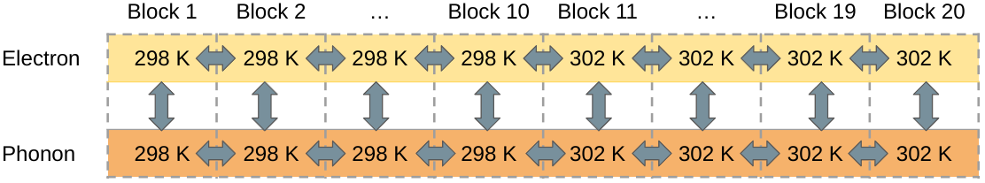
Figure 2: Network of local systems that show how the local electron and phonon systems interact within the SEAQT framework; the arrows indicate electron-electron, phonon-phonon, and electron-phonon interactions.

2.6 Transport properties

The electrical conductivity is defined based on Eq. (33) as

$$\sigma=\int\frac{\partial f}{\partial\epsilon}e^{2}\,v_{x}^{2}\tau^{\prime}(\epsilon)D(\epsilon)\,d\epsilon$$ (41)

where the BTE relaxation parameter, $\tau^{\prime}$, is related to the SEAQT relaxation parameter, $\tau^{\epsilon}$, via Eq. (34), $\delta x^{2}=V\delta x/A_{c}$, and the Fermi distribution is that for fermions given in Eq. (32).

The thermal conductivity $\kappa$ is expressed as

$$\kappa=\frac{1}{3}\int\tau^{\prime}v_{x}^{2}C_{\omega}d\omega$$ (42)

where the specific heat per unit frequency $C_{\omega}$ is given by

$$C_{\omega}=\hbar\omega D(\omega)\frac{\partial f}{\partial T}$$ (43)

and $\hbar$ is Planck’s modified constant. To determine the electron contribution to $\kappa$, the Fermi distribution for fermions (Eq. (32)) is used, while for the phonon contribution, the distribution for bosons (Eq. (37)) is employed. Note the the emperature $T$ is either the electron or the phonon temperature.

As to the Seebeck coefficient, it is given by

$$S=\frac{1}{eT}\frac{\int(\epsilon-\mu)(\partial f/\partial\epsilon)e^{2}\,v_{x}^{2}\tau^{\prime}(\epsilon)D(\epsilon)d\epsilon}{\sigma}$$ (44)

where $\mu$ is the chemical potential and $T$ the average of the electron and phonon temperatures.

Finally, the figure of merit, $ZT$, which is used to define the performance of semiconductors for thermoelectric applications, is given by

$$ZT=\frac{S^{2}\sigma T}{\kappa}$$ (45)

2.7 Energy landscape

Accurate energy landscapes for the electrons and phonons are needed as inputs to the SEAQT framework to produce accurate predictions of the transport and non-equilibrium intensive properties. The most common method for determining the electron energy landscape, i.e., the electron DOS, is density functional theory (DFT). This is the method used here directly using VASP and the Local Density Approximation (LDA) pseudo-potential for cell relaxation and static band structure calculations. Some of the electron DOS’s utilized are found from the literature.

To determine the phonon energy landscape, i.e., the phonon DOS, DFT can also be used, or it can be found from experiments. In addition, accurate calculations of the phonon relaxation parameter and phonon velocity are needed. Another method used for determining the phonon DOS of some of our materials is one based on elastic constants. This method utilizes the continuum elastic wave equation, i.e.,

$$\rho\frac{\partial^{2}R}{\partial t^{2}}=\nabla\cdot\boldsymbol{\sigma}$$ (46)

to obtain particle displacements that can then be used to find the phonon energy landscape. In this last equation, $\rho$ is the density of the material, $R$ the particle displacement, and $\boldsymbol{\sigma}$ the stress tensor. By knowing the elastic constants that go into forming the stress tensor, the degeneracy for a given frequency can be calculated using

$$g_{n}(\omega)=\frac{1}{t}\left[\frac{k_{n}(\omega)}{2\pi v_{n}(\omega)}\right]$$ (47)

In the last expression, $t\$is the thickness of the material, $k_{n}(\omega)$ the x-component of the wave vector for a given angular frequency, and $v_{n}(\omega)$ the group velocity given a specific angular frequency.

3 Results

In the following sections, results found utilizing the SEAQT framework are presented for the electrical and thermal conductivities, the Seebeck coefficient, and the figure of merit for a number of semiconductor materials including Si, doped Si, and Bi₂Te₃. Results for Ge are presented in the supplementary materials. For all the materials considered, the material systems analyzed utilize the network of local non-equilibrium systems shown in Fig. 2. Each simulation employs 20 blocks, each with a length of 1$\times 10^{-7}$ meters, the same crystal structure, and the same orientation. Each block consists of a local electron non-equilibrium system and a local phonon non-equilibrium system. Note that the crystal structures between block need not be the same such as when there are defects in certain blocks but not in others.

To find the total rate of change of the energy and mass in a given local system, the energy and mass flows with neighboring local systems at every instant of time must be determined. Thus, for instance, Electron-2 has three neighbors: Electron-1, Electron-3, and Phonon-2. To calculate the mass and energy flows from, for example, Electron-1 to Electron-2, the SEAQT equations of motion, Eqs. (19) and (20), are applied to a composite system of Electron-1 and Electron-2 subject to a specific set of constraints. The composite of Electron-1 and Electron-2 results in a ($m+m^{\prime}$)^th-order hypo-equilibrium description where $m$ is the number of eigenlevels in Electron-1 and $m^{\prime}$ the number in Electron-2. The mass and energy flows then result from the relaxation of the non-equilibrium composite system. Electron-electron transport is solved subject to the {$\tilde{C}(\gamma)$} = {$\tilde{H}$,$\tilde{N}$,${\tilde{I}}_{a}$,…,${\tilde{I}}_{m}$} constraints, phonon-phonon transport to the $\{\tilde{C}(\gamma)\}=\{\tilde{H},\tilde{I}_{a},\ldots,\tilde{I}_{m}\}$ constraints, and phonon-electron transport to the {$\tilde{C}(\gamma)$} = {$\tilde{H}$,$\tilde{N_{e}}$,${\tilde{I}}_{a}$,…,${\tilde{I}}_{m}$} constraints. In the latter case, the electron particle number is conserved, while the phonon particle number is not. All of this is repeated for the other pairings with Electron-3 and Phonon-2. This results is the total rate of change of the energy and mass of Electron-2. Using this procedure, the energy and mass flows in all of the local systems are determined and the whole network’s relaxation predicted.

Now, in order for the SEAQT code to run properly, a small induced temperature difference needs to be present for the equation of motion to run. Therefore, the temperature of the first 10 blocks is initially set to 298 K and that of the second 10 blocks to 302 K.

3.1 Bi₂Te₃

Bi₂Te₃ is used here as a case study to compare the SEAQT results to those produced by the BoltzTraP code. Due to the spin-orbit coupling between the Bi and Te atoms, Bi₂Te₃ takes on additional computational complexity relative to its electron DOS when compared to simpler semiconductor systems. VASP is used to determine this DOS, which is given in Fig. 4. In contrast, the phonon DOS seen in Fig. 4 is taken from first-principle DFT calculations found in [26]. In addition, as indicated above, the phonon relaxation parameter, $\tau^{\epsilon}$, is important in scaling the thermal conductivity of the material. This is especially true for an anisotropic material such as Bi₂Te₃ for which the thermal conductivity changes depending on the $xx$- or $zz$-directions (i.e., the transverse and longitudinal directions) [27]. This anisotropy affects the group velocities for the phonons. These are taken from reference [28] and shown in Table 1. The calculated phonon relaxation parameters, $\tau^{\epsilon}$, also appear in Table 1 and are based on the phonon velocities and a constant phonon relaxation parameter, $\tau^{\prime}$, of 2.2$\times 10^{-11}$ s taken from reference [29]. Per Eq. (34), these $\tau^{\epsilon}$ do not vary with the eigenenergies since $\tau^{\prime}$ does not in this case. As to the electron $\tau^{\epsilon}$, these are affected by the anisotropic change of the effective mass as well as by the eigenenergies (see Eq. (34)). These masses are

Table 1: Phonon velocities and calculated phonon relaxation parameters, $\tau^{\epsilon}$, for the $xx$- and $zz$-directions of the Bi₂Te₃ cell.

Direction	Phonon Velocity (m/s)	Phonon Relaxation Parameter, $\tau^{\epsilon}$ (s)
xx	1800	1.4$\times 10^{-10}$
zz	2600	6.7$\times 10^{-11}$

Table 2: Bi₂Te₃ electron effective masses for different directions.

Direction	Effective mass Conduction Band	Effective mass Valance Band
	(free electron mass)	(free electron mass)
xx	46.9	32.5
zz	9.5	9.02

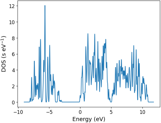
Figure 3: Electron DOS of Bi₂Te₃.

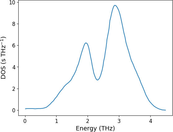
Figure 4: Phonon DOS of Bi₂Te₃ [26]

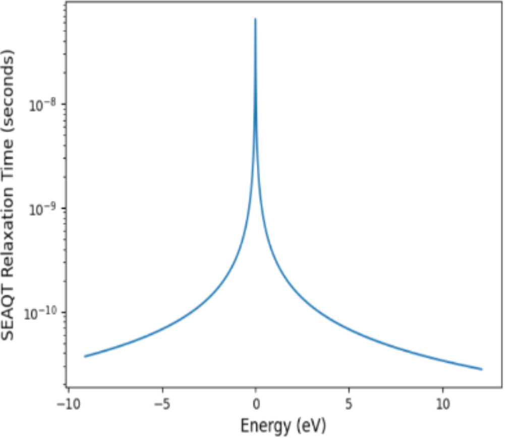
Figure 5: Calculated electron relaxation paramater, $\tau^{\epsilon}$ for Bi₂Te₃ in the xx-direction as a function of the eigenenergies.

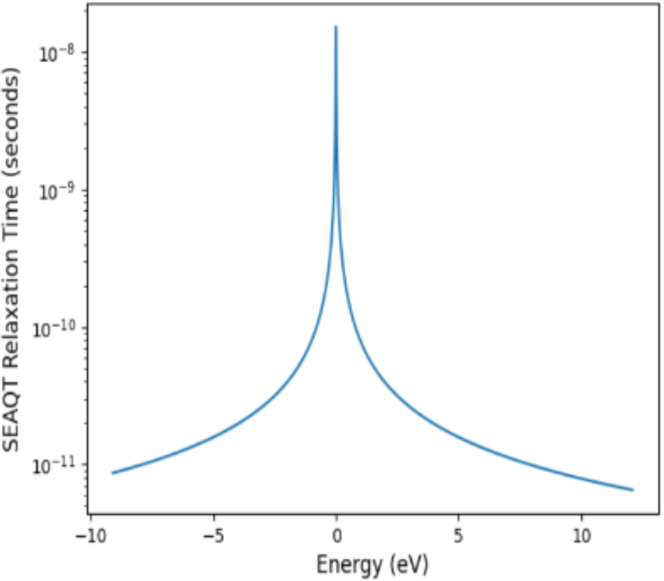
Figure 6: Calculated electron relaxation paramater, $\tau^{\epsilon}$ for Bi₂Te₃ in the zz-direction as a function of the eigenenergies.

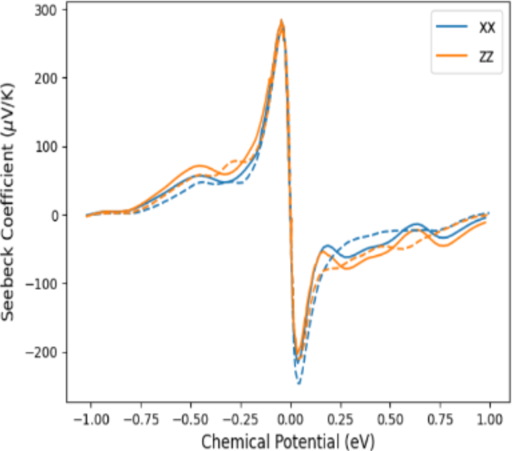
Figure 7: SEAQT Seebeck coefficient of Bi₂Te₃ in the $xx$ and $zz$ directions as a function of chemical potential; the dotted curves are the BoltzTrap predictions while the solid curves are those of the SEAQT framework.

given in Table 2 and are taken from [30]. Averaging the effective masses in each direction, the electron $\tau^{\epsilon}$ in the xx and zz directions as a function of the eigenenergy are reported in Figs. 6 and 6, repsectively.

Fig. 7 shows the SEAQT and Boltztrap Seebeck coefficients for the $xx$ or $zz$ directions, respectuvely. As can be seen, the Boltztrap and SEAQT predictions are in general agreement with each other. To determine the overall thermoelectric properties of the Bi₂Te₃, Matthiessen’s rule [31] is used to find an overall relaxation parameter, $\tau^{\epsilon}$, using the $xx$- and $zz$-direction relaxation parameters reported in Figs. 6 and 6. Fig. 8 shows that the SEAQT predictions, when compared to a number of different experimental studies [32, 33, 34, 35], capture the correct trends for the electrical and thermal conductivities, the Seebeck coefficient, and the figure of merit, i.e., the so-called $ZT$ factor. The values of these properties are also in general agreement with the experimental values although as can be seen there is quite a bit of spread between the various experimental values. For example, the SEAQT thermal conductivity (top right figure of Fig. 8) is shown to be somewhat higher compared to the experimental data. However, this discrepancy is due to the fact that the predicted values are based on a pure crystal structure without defects, while the experimental samples fabricated using a spark-plasma sintering method are not. The impacts of this fabrication method are explained in Section 4: Discussion. On the other hand, the comparison seen in Fig. 9 of SEAQT results for the phonon thermal conductivity (i.e., when the electron contribution is not considered) with both experimental [36, 37] and molecular dynamic [38] results shows quite good agreement. Note, however, that as is evident in Fig. 8, not including the electron contribution significantly under predicts the total thermal conductivity for a narrow-bandgap material such as Bi₂Te₃. Thus, being able to account for both the electron as well as the phonon contributions simultaneously is important.

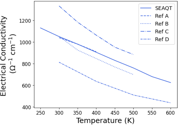
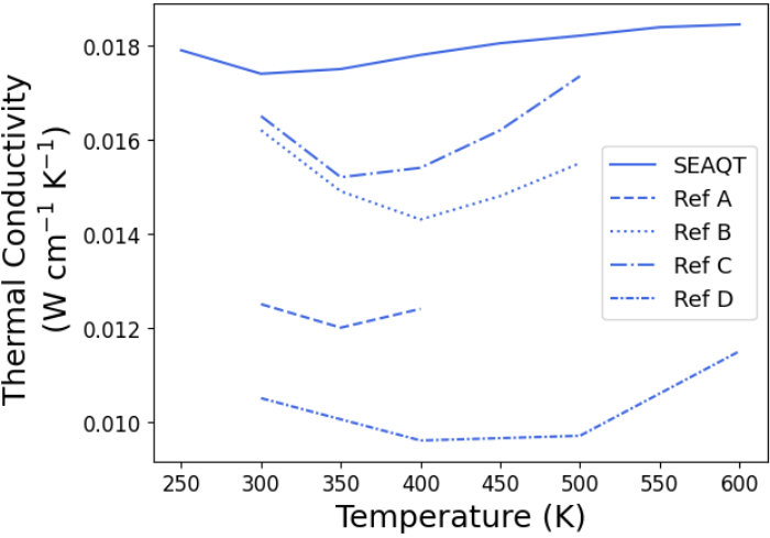
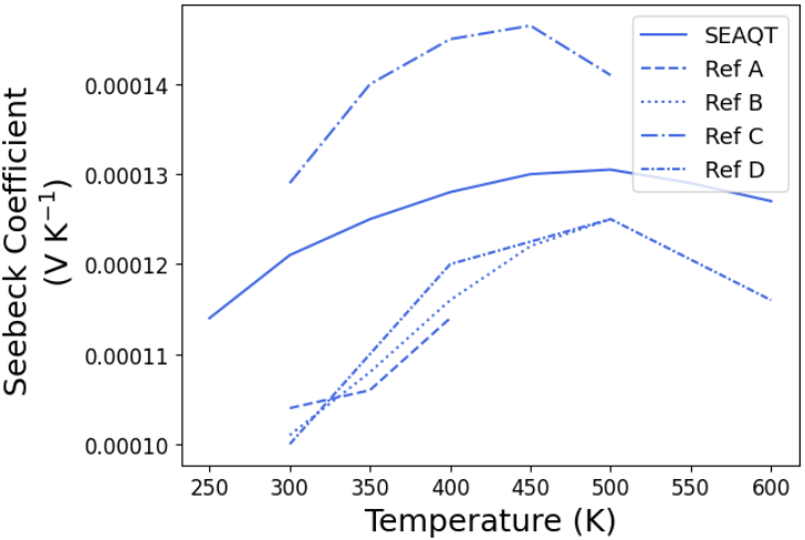
Figure 8: (top left) Comparison of the SEAQT results for the electrical conductivity, (top right) thermal conductivity, (bottom left) Seebeck coefficient, (bottom right) and the $ZT$ factor of Bi₂Te₃ with experimental data; Ref A is [32], Ref B is [33], Ref C is [34], Ref D is [35].

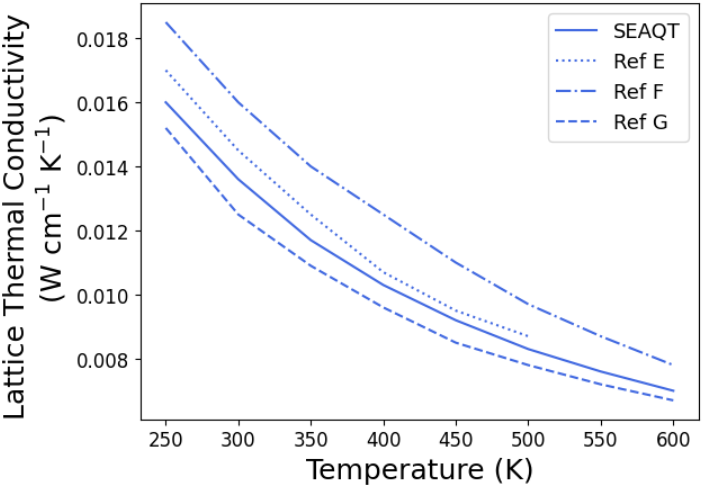
Figure 9: SEAQT Bi₂Te₃ phonon thermal conductivity results compared with experimental and molecular dynamic results; Ref E is [38], Ref F is [36], Ref G is [37].

3.2 Si and Ge

Both Si and Ge are semiconductor materials that have been highly studied both experimentally and computationally [39, 40, 41]. SEAQT results for Ge and comparisons with data found in the literature are given in the $Supplementary\;Materials$. The electron DOS for Si and for Ge is calculated using VASP’s DFT calculations [42, 43, 44]. For both materials, the Local Density Approximation (LDA) pseudopotential is used along with the hybrid HSE03 functional to correct for the inherent band gap problem in modeling these two semiconductors. Although not shown here, the electron DOS obtained with VASP given in Fig. 10 is comparable to computations found in the literature [45].

As to the Si phonon DOS shown on the right in Fig. 10, it is determined using the method of elastic constants and the elastic wave equation (Eq. (46)) briefly discussed in Section 2.7. Due to the material being isotropic, the direction does not impact the relaxation parameter of electrons, which is shown as a function of the eigenenergies in Fig. 11. These values are applicable for the doped Si as well since doping has a negligible effect on $\tau^{\epsilon}$. The direction also does not impact the phonons where we consider the [1,0,0] direction and take the group velocity and relaxation parameter from [46]. The values used are 6791 m/s and 3.8 ns, respectively [47, 48]. Fig. 12 shows that the SEAQT predictions, when compared to a number of different experimental studies [39, 40, 41], capture the values and trends for the electrical and thermal conductivities, the Seebeck coefficient, and the figure of merit, $ZT$, very well. BoltzTraP predictions for the electrical conductivity and the Seebeck coefficient are also shown and compare much less favorably with the experimental data. Two BoltzTraP curves are shown for the electrical conductivity: one (upper curve) based on the constant relaxation parameter of 10^-14 s typically used by BoltzTraP and the other (lower curve) on 10^-15 s, which is a value sometimes used by BoltzTraP. The Seebeck coefficient shows only one BoltzTraP curve because there is no substantial difference between the curves at the different relaxation parameter values.

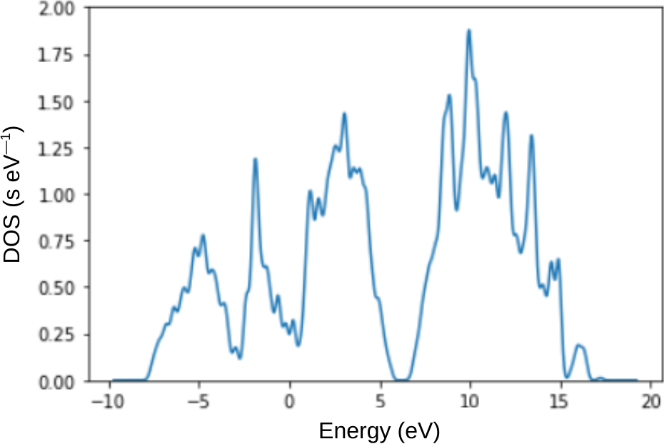
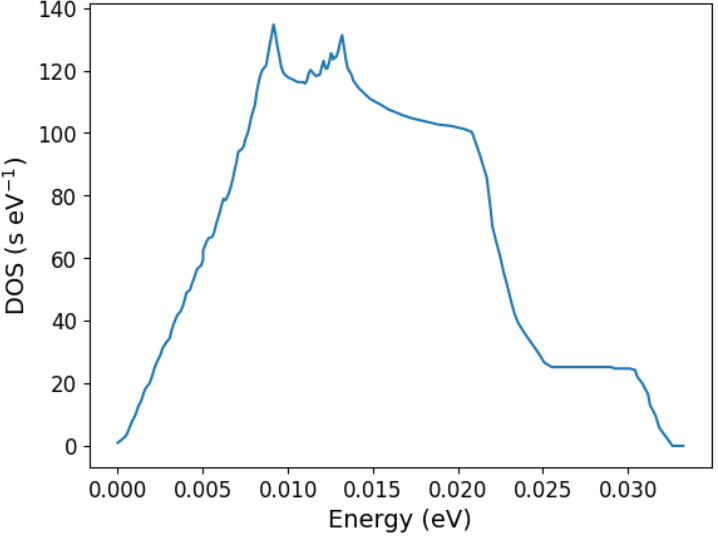
Figure 10: (left) Electron DOS and (right) phonon DOS for Si.

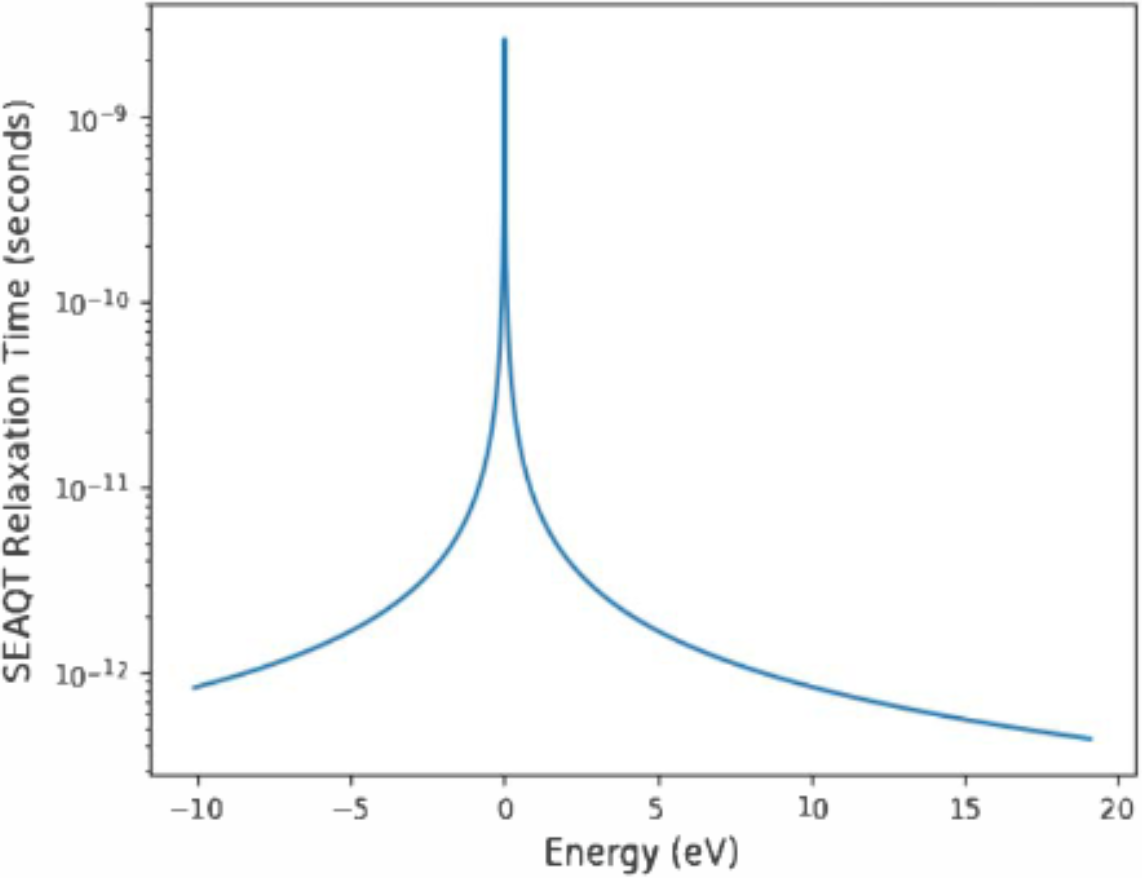
Figure 11: Calculated electron relaxation parameter, $\tau^{\epsilon}$, for Si and doped Si as a function of the eigenenergies.

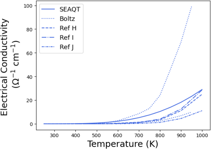
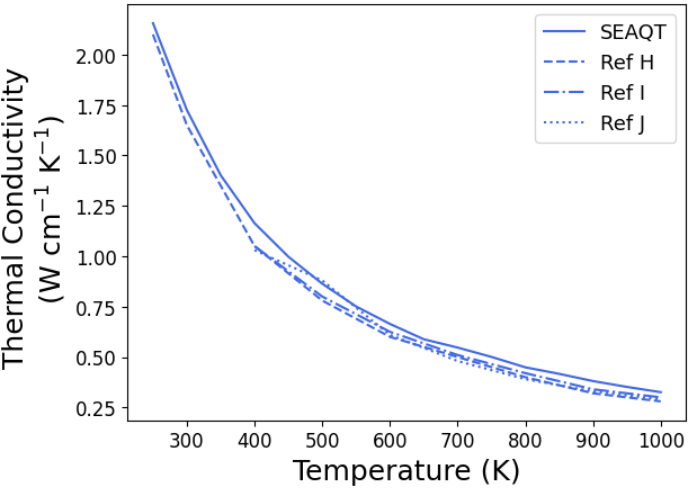
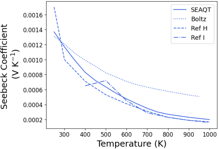
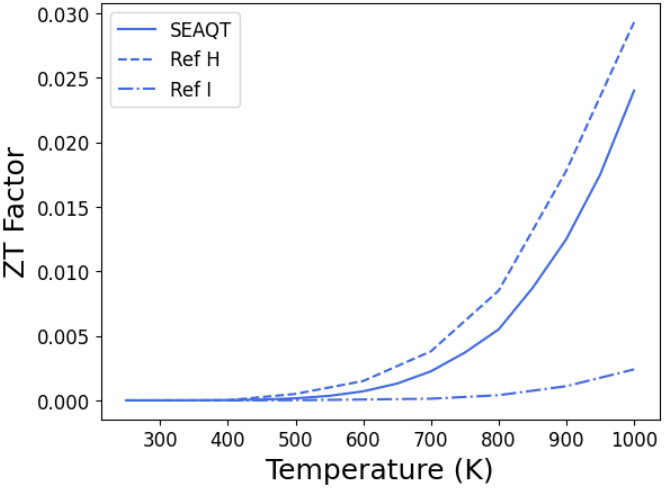
Figure 12: (top left) Comparison of the SEAQT results for the electrical conductivity, (top right) thermal conductivity, (bottom left) Seebeck coefficient, and (bottom right) $ZT$ factor of Si with BoltzTraP and experimental data; Ref H is [39], Ref I is [40], Ref J is [41].

3.3 Doped Si

Consistent with BoltzTrap, it is assumed here that the doping levels of Si do not substantially impact the electron DOS but can be taken into account by adjusting the Fermi level depending on the level of doping present [49]. This change in Fermi level is important to modeling the change in transport properties of the doped Si with the SEAQT framework. The change in Fermi level is taken from the BoltzTraP code that determines this change on the basis of the additional charge carriers of the doping material [50]. The doping levels are chosen based on the experimental n and p-type doping levels to which our predicted results are to be compared [51]. The concentration of dopants studied here also does not substantially adjust the phonon DOS. The primary change in phonon transport properties comes from the change in the phonon relaxation due to the additional scattering by impurities, free electrons/holes, and bound electrons/holes. The calculated phonon relaxation parameters are given in Table 3 [52]. As can be seen in Fig. 13, the predicted SEAQT values for the electrical conductivity and Seebeck coefficient are in good agreement with the experimental results, while the BoltzTrap results are not. The SEAQT predictions for the thermal conductivity, which include contributions from both the electrons and phonons, are given in the middle figure on the left in Fig. 13. SEAQT results for the n-doping with Phosphorus and the p-doping with Boron follow the experimental values quite well with the largest deviation occurring for the case of the smallest n-doping (light blue curves). Furthermore, since Si is a conventional and not a narrow-bandgap semiconductor, the contribution to the thermal conductivity from the electrons is much smaller than was the case for Bi₂Te₃. This can be seen in Fig. 14 where the thermal conductivity due to the electrons only is small compared to the total thermal conductivity of Fig. 13 and increases as expected with increased doping as does the electrical conductivity.

Table 3: Doped Si Relaxation Parameters.

Doping and Concentration	Relaxation Parameter (ns)
p-type 2$\times 10^{16}$	3.618
p-type 1$\times 10^{20}$	1.761
n-type 2$\times 10^{17}$	3.472
n-type 1$\times 10^{18}$	2.312
n-type 2$\times 10^{19}$	2.002
n-type 1$\times 10^{20}$	1.498

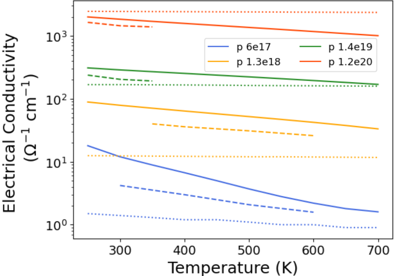
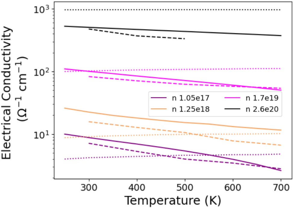
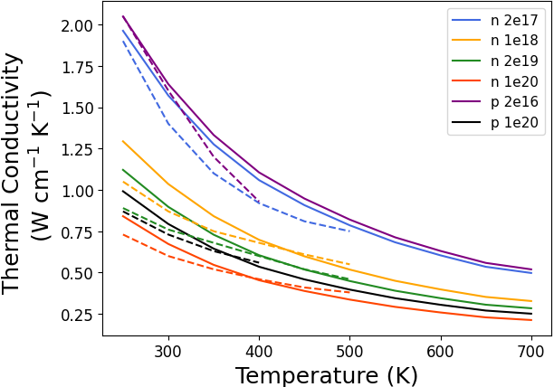
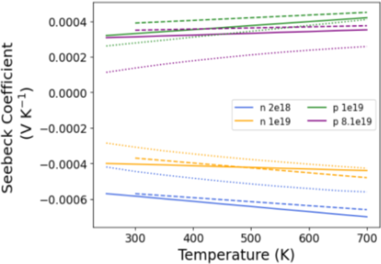
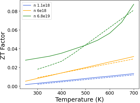
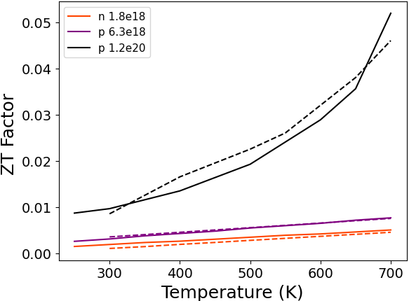
Figure 13: (top left and right) Comparisons of the SEAQT results (solid curves) for the electrical conductivity [51], (middle left) thermal conductivity [52], (middle right) Seebeck coefficient [53], and (bottom left and right) $ZT$ factor [54] of doped Si with experimental data (dashed curves). BoltzTraP predictions (dotted curves) are given as well using the BoltzTraP value for the relaxation parameter of $10^{-14}$ s.

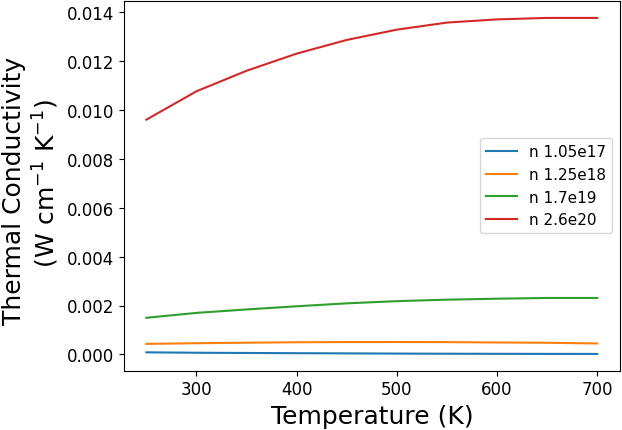
Figure 14: Electron thermal conductivity of doped Si.

4 Discussion

The electrical conductivity and Seebeck coefficient are dependent on the mobility of electrons and electron holes, which are controlled by the Fermi level in semiconductors. At 0 K, electrons remain in the valance band and do not move toward the conduction band. With increasing temperature, the Fermi level increases, resulting in some electrons moving into the conduction band and leaving behind holes in the valance band. This contributes to electrical conductivity. As for the Seebeck coefficient, the induced voltage caused by a temperature gradient is due to the fact that electrons are electrical and thermal carriers. With an induced temperature gradient, electrons move from a high temperature regions to a low temperature ones, resulting in an electric current [55]. The magnitude and sign of the Seebeck coefficient are related to an asymmetry of the electron distribution around the Fermi level. Thus, changes in the Fermi level with temperature not only adjust the electron and hole concentration but as well the Seebeck coefficient magnitude (via concentration increases/decreases and electron/hole mobility) and sign (via excess electrons for n-type materials and excess holes for p-type materials) [56, 57].

It is important to show the validity and reliability of the SEAQT model by comparing its predicted results to those of standard methods. In the case of this paper, SEAQT results are compared to those of BoltzTraP based on VASP generated electron DOS. Predicted results are also compared to experimental data. For Bi₂Te₃, SEAQT results are compared to experimental data in Fig. 8. The electrical conductivity, Seebeck coefficient, and $ZT$ factor are in good agreement with the provided references where the SEAQT data is generally the average of the experimental values. The spread in the experimental values are likely due to the fabrication method that is explained below. This is also the case for the thermal conductivity where the SEAQT values are higher compared to the spread in the experimental values. However, the SEAQT lattice thermal conductivity, which only considers the phonon contribution, compares well with the experimental results shown in Fig. 9. This suggest that there is a significant electron contribution to the total thermal conductivity (Fig. 8), which is consistent with the fact that Bi₂Te₃ is a narrow-bandgap semiconductor.

For Si, both SEAQT and BoltzTraP results are compared to experimental data as shown in Fig. 12. For the electrical conductivity, BoltzTraP results show two curves as an upper and lower limit on possible constant electron relaxation parameters given here to be either 10^-14 or 10^-15 s. The increasing trends and magnitudes of the experimental data are similar to those predicted by the SEAQT framework and in between those predicted by BoltzTraP. The SEAQT predicted Seebeck coefficient is in very close agreement with the experimental data, while the BoltzTraP predictions deviate from the experimental particularly at higher temperatures. As to the SEAQT predictions of the thermal conductivity, they are in very close agreement with the experimental data as are the SEAQT $ZT$ factor results.

Both SEAQT result and BoltzTraP results with a constant relaxation parameter of 10^-14 s are compared to experimental data for doped Si in Fig. 13. The SEAQT results for the electrical conductivity compare very well with the experimental data showing similar magnitudes and a decreasing trend of electrical conductivity with increasing temperature. In contrast, the BoltzTraP results for electrical conductivity do not compare well to the experimental data where, depending on the doping level, the results do not have the correct magnitudes nor do they display a decrease in the electrical conductivity with increasing temperature. The Seebeck coefficient shows similar issues where the SEAQT results are closer to the experimental data than those of BoltzTraP. However, both the SEAQT and BoltzTraP results show the correct n-type and p-type negativity and positivity, respectively. As to the thermal conductivity, the SEAQT results decrease with increasing doping concentrations due to the adjusted relaxation parameters from the scattering mechanisms of the impurity atoms. There are slight discrepancies between the SEAQT results and experimental data where the SEAQT values are greater. This could potentially be due to the adjustment of the relaxation parameter or the DOS not including other defects that could be present in the experimental samples such as dislocations that would impact the thermal conductivity. Even with these slight discrepancies, the SEAQT $ZT$ factor matches very well with the experimental data for all the given doping levels.

An obvious limitation of the BoltzTraP method results from the use of a constant relaxation parameter model that leads to an overestimation or an underestimation of the electrical conductivity. The largest disparities occur for doped Si (Fig. 13). At lower doping levels, such as n-doped 1.05$\times 10^{17}$ 1/cm³, the BoltzTraP electrical conductivity is close to the experimental value, but does not have the correct trend of decreasing electrical conductivity with increasing temperature. At higher doping levels, such as n-doped 2.6$\times 10^{20}$ 1/cm³, the BoltzTraP value is approximately higher or lower by a factor of 5 from the experimental and SEAQT values. This over or under estimation of the electrical conductivity by BoltzTraP could be due to the exclusion of the electron-phonon coupling that influences electron mobility. Generally, electron-phonon scattering results in lower electron mobility, directly reducing the electrical conductivity [58]. When analyzing the Seebeck coefficient, SEAQT analysis of doped Si (Fig. 13) reproduces the experimental values much more accurately than BoltzTraP. This is due in part to the constant relaxation parameter approximation employed by BoltzTraP that is generally only appropriate when the relaxation parameter is not energy dependent [59]. However, when it is, the measured Seebeck coefficient can deviate significantly from a model such as that employed by BoltzTraP. This issue is addressed in the SEAQT framework, which accounts for this energy dependency as well as the electron-phonon coupling.

As to the thermal conductivity for the doped Si, it consists of a phonon contribution, $\kappa_{l}$ and an electron contribution, $\kappa_{e}$. The latter is proportional to the electrical conductivity, $\sigma$, via the Lorentz number such that

$$\frac{\kappa_{e}}{\sigma}=LT$$ (48)

where $T\$is the temperature and $L\$ the Lorentz number that ranges approximately from $2.4\,\times\,10^{-8}$ $W\Omega K^{2}$ for degenerate semiconductors to $1.5\times 10^{-8}$ $W\Omega K^{2}$ for non-degenerate semiconductors [60, 61]. The total thermal conductivity is given by

$$\kappa_{tot}=\kappa_{l}+\kappa_{e}$$ (49)

As can be seen from both of these equations, at lower electrical conductivities, the electron contribution to the thermal conductivity remains low but increases with increasing doping levels that correspond to increasing electrical conductivity. Fig. 13 shows that although an increase in the doping results in an increase in the electrical conductivity, the increase is not enough to substantially impact the total thermal conductivity of the doped Si significantly. As mentioned early, this was not the case for Bi₂Te₃, which did see a substantial electron contribution.

A unique characteristic of the SEAQT framework when compared to other computational models is its ability to simultaneously determine all the thermoelectric properties of a material and, thus, its figure of merit. The SEAQT frameowrk is, therefore, able to produce results in closer agreement with experimental data than, for example, the current state-of-the-art BoltzTraP code. Furthermore, for materials with inherent defects that cause additional scattering of electrons and phonons [62, 63], the SEAQT framework via a network of local non-equilibrium systems is able to computationally account for the effects of these defects on the thermoelectric properties of the materials. This is an important feature because one-dimensional (vacancies, interstitial atoms, substitutional atoms, line dislocations), two-dimensional (stacking faults, grain boundaries, twin boundaries), and three-dimensional (precipitates, intermetallic phases, pores, cracks) defects increase the scattering mechanisms with increasing defect dimension and concentration [62, 63]. Vacancy clusters are known to impact electrical conductivity due to dangling bonds, floating bonds, and high strain atoms that generate a localized state where electrons are confined to a certain region, causing the material to behave like a metal and increasing lower frequency phonons, while decreasing phonon velocities [64]. Dislocations interfere with the symmetry of a perfect crystal, changing the band gap energy and affecting the electrical conductivity due to the dislocation acting either as an acceptor or donor [65]. In addition, the thermal conductivity decreases with dislocation density and with the magnitude of change of single dislocations being dependent on the orientation in the lattice [66]. These defects could potentially explain the higher SEAQT thermal conductivity of Bi₂Te₃ shown in Fig. 8 where the experimental samples would have higher inherent defects, such as line dislocations and grain boundaries, that reduce thermal conductivity in the experimental samples. Separating the SEAQT Bi₂Te₃ thermal conductivity into its lattice and electron contributions as is done in Eq. (8), the lattice conductivity matches well with the experimental and molecular dynamics simulations shown in the Fig. 9 that result from very pure samples and idealized simulation conditions. The fact that the experimental thermal conductivity values of some of the samples in Fig. 8 are much lower at low temperatures than the experimental phonon thermal conductivity data in Fig. 9 can be attributed to the reduction of the phonon contribution due to the phonon scattering on grain boundaries and dislocations of the samples of Fig. 8 [32]. These defects are inherent to the type of fabrication process. The Bi₂Te₃ samples of Fig. 8 were fabricated using the spark plasma sintering (SPS) method [32, 33, 34, 35]. Making defect-free materials produced from SPS is extremely difficult due to the many separate mechanisms that need to be controlled to adjust the microstructure. These include temperature inhomogeneities due to complex current distribution, non-uniform stress distributions, die material, applied electric field, applied pressure, and heating rates [67]. It is incredibly difficult to adjust these specific mechanisms for fabricating pure, bulk materials as understanding what mechanisms control which microstructures is still being researched with the main theories being plasma generation, electroplastic effect, and joule heating [67, 68]. As a result, SPS leads to materials with inherent defects that change the thermoelectric properties compared to single-crystal materials. This issue primarily arises with small grain sizes that are inherent with the SPS method due to the micropowder that is sintered, leading to much lower thermal conductivities compared to single-crystal samples [68]. The SEAQT framework can be appropriately adjusted to account for these defects by changing the input parameters appropriately. In this case, the DOS of the materials can be obtained through experimental methods or the use of computational methods such as DFT with imputed defects to obtain an adjusted electron/phonon DOS as well as adjusted relaxation parameters and group velocities.

5 Conclusions

Utilization of the SEAQT framework is shown to accurately reproduce the experimental results of semiconductor materials. SEAQT takes into account electron and phonon energy landscapes to determine material transport properties that cannot be determined by current computational/physical methods. This framework inherently satisfies the laws of quantum mechanics and thermodynamics, utilizing an equation of motion to determine unique non-equilibrium thermodynamic paths through Hilbert space and is able to cross several spatial and temporal scales in a single analysis.

The SEAQT framework has been used here to determine the transport properties of Bi₂Te₃, Si, and doped Si (as well as Ge in the $Supplementary\>Materials$) with good accuracy. It provides results similar to the current computational and physical standards, while taking into account the coupling of electron and phonon phenomena to provide more accurate results. The robustness of the SEAQT framework is such that it can be applied to a multitude of systems and will be used to analyze the effect of defect structures and the thermoelectric breakdown of materials in future work.

6 Declaration of Competing Interests

The authors declare no competing interest.

Supplementary Information is available for this paper.

CRediT Author Statement: Jarod Worden: software, validation, formal analysis, investigation, data curation, writing - original draft, writing - review and editing, visualization Micheal von Spakovsky: conceptualization, methodology, resources, writing - review and editing, supervision, project administration, funding acquisition Celine Hin: writing - review and editing, supervision, project administration

References

- [1] C. Cercignani and A.. Berman “Theory and Application of the Boltzmann Equation” Number: 3 Code: Journal of Applied Mechanics In Journal of Applied Mechanics 43.3, 1976, pp. 521–521 DOI: 10.1115/1.3423913
- [2] M… Newman and G.. Barkema “Monte Carlo methods in statistical physics” Oxford : New York: Clarendon Press ; Oxford University Press, 1999
- [3] D.. Rapaport, Robin L. Blumberg, Susan R. McKay and Wolfgang Christian “The Art of Molecular Dynamics Simulation” Number: 5 Code: Computers in Physics In Computers in Physics 10.5, 1996, pp. 456 DOI: 10.1063/1.4822471
- [4] Wm.G. Hoover “Nonequilibrium molecular dynamics” Number: 1-2 Code: Nuclear Physics A In Nuclear Physics A 545.1-2, 1992, pp. 523–536 DOI: 10.1016/0375-9474(92)90490-B
- [5] David Jou and Georgy Lebon “Extended Irreversible Thermodynamics” Code: Extended Irreversible Thermodynamics Publication Title: Extended Irreversible Thermodynamics Reporter: Extended Irreversible Thermodynamics Dordrecht: Springer Netherlands, 2010 DOI: 10.1007/978-90-481-3074-0
- [6] S.. Groot and P. Mazur “Non-equilibrium thermodynamics” Code: Non-equilibrium thermodynamics Publication Title: Non-equilibrium thermodynamics Reporter: Non-equilibrium thermodynamics New York: Dover Publications, 1984
- [7] P. Vogl and T. Kubis “The non-equilibrium Green’s function method: an introduction” Number: 3-4 In Journal of Computational Electronics 9.3-4, 2010, pp. 237–242 DOI: 10.1007/s10825-010-0313-z
- [8] Naoaki Kondo, Takahiro Yamamoto and Kazuyuki Watanabe “Molecular-dynamics simulations of thermal transport in carbon nanotubes with structural defects” Number: 0 In e-Journal of Surface Science and Nanotechnology 4.0, 2006, pp. 239–243 DOI: 10.1380/ejssnt.2006.239
- [9] Mie Andersen, Chiara Panosetti and Karsten Reuter “A Practical Guide to Surface Kinetic Monte Carlo Simulations” In Frontiers in Chemistry 7, 2019, pp. 202 DOI: 10.3389/fchem.2019.00202
- [10] G. Chen “Thermal conductivity and ballistic-phonon transport in the cross-plane direction of superlattices” Number: 23 In Physical Review B 57.23, 1998, pp. 14958–14973 DOI: 10.1103/PhysRevB.57.14958
- [11] Guanchen Li, Michael R. Spakovsky and Celine Hin “Steepest entropy ascent quantum thermodynamic model of electron and phonon transport” Number: 2 In Physical Review B 97.2, 2018, pp. 024308 DOI: 10.1103/PhysRevB.97.024308
- [12] G.. Beretta, E.. Gyftopoulos, J.. Park and G.. Hatsopoulos “Quantum thermodynamics. A new equation of motion for a single constituent of matter” Number: 2 Code: Il Nuovo Cimento B Series 11 In Il Nuovo Cimento B Series 11 82.2, 1984, pp. 169–191 DOI: 10.1007/BF02732871
- [13] Gian Paolo Beretta “Nonlinear quantum evolution equations to model irreversible adiabatic relaxation with maximal entropy production and other nonunitary processes” Number: 1-2 Code: Reports on Mathematical Physics In Reports on Mathematical Physics 64.1-2, 2009, pp. 139–168 DOI: 10.1016/S0034-4877(09)90024-6
- [14] Gian Paolo Beretta “Steepest entropy ascent model for far-nonequilibrium thermodynamics: Unified implementation of the maximum entropy production principle” Number: 4 In Physical Review E 90.4, 2014, pp. 042113 DOI: 10.1103/PhysRevE.90.042113
- [15] Guanchen Li and Michael R. Spakovsky “Steepest-entropy-ascent quantum thermodynamic modeling of the relaxation process of isolated chemically reactive systems using density of states and the concept of hypoequilibrium state” Number: 1 Code: Physical Review E In Physical Review E 93.1, 2016, pp. 012137 DOI: 10.1103/PhysRevE.93.012137
- [16] Guanchen Li and Michael R. Spakovsky “Generalized thermodynamic relations for a system experiencing heat and mass diffusion in the far-from-equilibrium realm based on steepest entropy ascent” Number: 3 In Physical Review E 94.3, 2016, pp. 032117 DOI: 10.1103/PhysRevE.94.032117
- [17] Guanchen Li and Michael R. Spakovsky “Modeling the nonequilibrium effects in a nonquasi-equilibrium thermodynamic cycle based on steepest entropy ascent and an isothermal-isobaric ensemble” Code: Energy In Energy 115, 2016, pp. 498–512 DOI: 10.1016/j.energy.2016.09.010
- [18] Guanchen Li and Michael R. Spakovsky “Steepest-entropy-ascent model of mesoscopic quantum systems far from equilibrium along with generalized thermodynamic definitions of measurement and reservoir” Number: 4 Code: Physical Review E In Physical Review E 98.4, 2018, pp. 042113 DOI: 10.1103/PhysRevE.98.042113
- [19] Guanchen Li, Omar Al-Abbasi and Michael R Spakovsky “Atomistic-level non-equilibrium model for chemically reactive systems based on steepest-entropy-ascent quantum thermodynamics” Code: Journal of Physics: Conference Series In Journal of Physics: Conference Series 538, 2014, pp. 012013 DOI: 10.1088/1742-6596/538/1/012013
- [20] Georg K.H. Madsen and David J. Singh “BoltzTraP. A code for calculating band-structure dependent quantities” Number: 1 Code: Computer Physics Communications In Computer Physics Communications 175.1, 2006, pp. 67–71 DOI: 10.1016/j.cpc.2006.03.007
- [21] Giovanni Pizzi, Dmitri Volja, Boris Kozinsky, Marco Fornari and Nicola Marzari “BoltzWann: A code for the evaluation of thermoelectric and electronic transport properties with a maximally-localized Wannier functions basis” Number: 1 Code: Computer Physics Communications In Computer Physics Communications 185.1, 2014, pp. 422–429 DOI: 10.1016/j.cpc.2013.09.015
- [22] Xufeng Wang, Evan Witkoske, Jesse Maassen and Mark Lundstrom “LanTraP: A code for calculating thermoelectric transport properties with the Landauer formalism” Issue: arXiv:1806.08888 arXiv:1806.08888 [cond-mat, physics:physics] arXiv, 2020 URL: http://arxiv.org/abs/1806.08888
- [23] Aidan P. Thompson, H. Aktulga, Richard Berger, Dan S. Bolintineanu, W. Brown, Paul S. Crozier, Pieter J. In ’T Veld, Axel Kohlmeyer, Stan G. Moore, Trung Dac Nguyen, Ray Shan, Mark J. Stevens, Julien Tranchida, Christian Trott and Steven J. Plimpton “LAMMPS - a flexible simulation tool for particle-based materials modeling at the atomic, meso, and continuum scales” In Computer Physics Communications 271, 2022, pp. 108171 DOI: 10.1016/j.cpc.2021.108171
- [24] Atsushi Togo, Laurent Chaput, Terumasa Tadano and Isao Tanaka “Implementation strategies in phonopy and phono3py” Issue: arXiv:2301.05784 arXiv:2301.05784 [cond-mat] arXiv, 2023 URL: http://arxiv.org/abs/2301.05784
- [25] Yan Wang, Xiulin Ruan and Ajit K. Roy “Two-temperature nonequilibrium molecular dynamics simulation of thermal transport across metal-nonmetal interfaces” Number: 20 In Physical Review B 85.20, 2012, pp. 205311 DOI: 10.1103/PhysRevB.85.205311
- [26] Shen Li and Clas Persson “Thermal Properties and Phonon Dispersion of Bi2Te3 and CsBi4Te6 from First-Principles Calculations” In Journal of Applied Mathematics and Physics 03.12, 2015, pp. 1563–1570 DOI: 10.4236/jamp.2015.312180
- [27] Olle Hellman and David A. Broido “Phonon thermal transport in Bi 2 Te 3 from first principles” Number: 13 In Physical Review B 90.13, 2014, pp. 134309 DOI: 10.1103/PhysRevB.90.134309
- [28] Jamal Alnofiay “Brillouin Light Scattering Studies of Topological Insulators Bi2Se3 , Sb2Te3 , and Bi2Te3”, 2014
- [29] Tianli Feng and Xiulin Ruan “Prediction of Spectral Phonon Mean Free Path and Thermal Conductivity with Applications to Thermoelectrics and Thermal Management: A Review” In Journal of Nanomaterials 2014, 2014, pp. 1–25 DOI: 10.1155/2014/206370
- [30] P. Larson, S.. Mahanti and M.. Kanatzidis “Electronic structure and transport of Bi 2 Te 3 and BaBiTe 3” Number: 12 In Physical Review B 61.12, 2000, pp. 8162–8171 DOI: 10.1103/PhysRevB.61.8162
- [31] Gang Chen “Nanoscale energy transport and conversion: a parallel treatment of electrons, molecules, phonons, and photons”, MIT-Pappalardo series in mechanical engineering Oxford ; New York: Oxford University Press, 2005
- [32] Zhen-Hua Ge, Yi-Hong Ji, Yang Qiu, Xiaoyu Chong, Jing Feng and Jiaqing He “Enhanced thermoelectric properties of bismuth telluride bulk achieved by telluride-spilling during the spark plasma sintering process” In Scripta Materialia 143, 2018, pp. 90–93 DOI: 10.1016/j.scriptamat.2017.09.020
- [33] D. Li, X.. Qin, Y.. Dou, X.. Li, R.. Sun, Q.. Wang, L.. Li, H.. Xin, N. Wang, N.. Wang, C.. Song, Y.. Liu and J. Zhang “Thermoelectric properties of hydrothermally synthesized Bi2Te3-xSex nanocrystals” Number: 2 In Scripta Materialia 67.2, 2012, pp. 161–164 DOI: 10.1016/j.scriptamat.2012.04.005
- [34] O.. Ivanov, M.. Yapryntsev, A.. Vasil’ev, M.. Zhezhu and V.. Khovailo “Metal-Ceramic Composite Bi2Te3–Gd: Thermoelectric Properties” Number: 5 In Glass and Ceramics 79.5, 2022, pp. 180–184 DOI: 10.1007/s10717-022-00480-7
- [35] Maxim Yaprintsev, Roman Lyubushkin, Oxana Soklakova and Oleg Ivanov “Effects of Lu and Tm Doping on Thermoelectric Properties of Bi2Te3 Compound” Number: 2 In Journal of Electronic Materials 47.2, 2018, pp. 1362–1370 DOI: 10.1007/s11664-017-5940-8
- [36] C.. Satterthwaite and R.. Ure “Electrical and Thermal Properties of Bi 2 Te 3” Number: 5 In Physical Review 108.5, 1957, pp. 1164–1170 DOI: 10.1103/PhysRev.108.1164
- [37] H J Goldsmid “The Thermal Conductivity of Bismuth Telluride” Number: 2 In Proceedings of the Physical Society. Section B 69.2, 1956, pp. 203–209 DOI: 10.1088/0370-1301/69/2/310
- [38] Bo Qiu and Xiulin Ruan “Molecular dynamics simulations of lattice thermal conductivity of bismuth telluride using two-body interatomic potentials” Number: 16 In Physical Review B 80.16, 2009, pp. 165203 DOI: 10.1103/PhysRevB.80.165203
- [39] Lois D’abbadie “Enhancement of the figure of merit of silicon germanium thin films for thermoelectric applications”, 2013 DOI: 10.26190/UNSWORKS/16828
- [40] W. Fulkerson, J.. Moore, R.. Williams, R.. Graves and D.. McElroy “Thermal Conductivity, Electrical Resistivity, and Seebeck Coefficient of Silicon from 100 to 1300°K” Number: 3 In Physical Review 167.3, 1968, pp. 765–782 DOI: 10.1103/PhysRev.167.765
- [41] H.. Shanks, P.. Maycock, P.. Sidles and G.. Danielson “Thermal Conductivity of Silicon from 300 to 1400°K” Number: 5 In Physical Review 130.5, 1963, pp. 1743–1748 DOI: 10.1103/PhysRev.130.1743
- [42] G. Kresse and J. Hafner “Ab initio molecular dynamics for liquid metals” Number: 1 In Physical Review B 47.1, 1993, pp. 558–561 DOI: 10.1103/PhysRevB.47.558
- [43] G. Kresse and J. Furthmüller “Efficiency of ab-initio total energy calculations for metals and semiconductors using a plane-wave basis set” Number: 1 In Computational Materials Science 6.1, 1996, pp. 15–50 DOI: 10.1016/0927-0256(96)00008-0
- [44] G. Kresse and J. Furthmüller “Efficient iterative schemes for ab initio total-energy calculations using a plane-wave basis set” Number: 16 In Physical Review B 54.16, 1996, pp. 11169–11186 DOI: 10.1103/PhysRevB.54.11169
- [45] “Density of States calculation • Quantum Espresso Tutorial.” URL: https://pranabdas.github.io/espresso/hands-on/dos/
- [46] Asegun S. Henry and Gang Chen “Spectral Phonon Transport Properties of Silicon Based on Molecular Dynamics Simulations and Lattice Dynamics” Number: 2 In Journal of Computational and Theoretical Nanoscience 5.2, 2008, pp. 141–152 DOI: 10.1166/jctn.2008.2454
- [47] David Lacroix, I. Traore, Sébastien Fumeron and G. Jeandel “Phonon transport in silicon, influence of the dispersion properties choice on the description of the anharmonic resistive mechanisms” In Physics of Condensed Matter 67, 2009, pp. 15–25 DOI: 10.1140/epjb/e2008-00464-6
- [48] A. Ward and D.. Broido “Intrinsic phonon relaxation times from first-principles studies of the thermal conductivities of Si and Ge” Number: 8 Publisher: American Physical Society In Physical Review B 81.8, 2010, pp. 085205 DOI: 10.1103/PhysRevB.81.085205
- [49] W Walukiewicz “Intrinsic limitations to the doping of wide-gap semiconductors” In Physica B: Condensed Matter 302-303, 2001, pp. 123–134 DOI: 10.1016/S0921-4526(01)00417-3
- [50] Georg K.H. Madsen, Jesús Carrete and Matthieu J. Verstraete “BoltzTraP2, a program for interpolating band structures and calculating semi-classical transport coefficients” In Computer Physics Communications 231, 2018, pp. 140–145 DOI: 10.1016/j.cpc.2018.05.010
- [51] G.. Pearson and J. Bardeen “Electrical Properties of Pure Silicon and Silicon Alloys Containing Boron and Phosphorus” Number: 5 In Physical Review 75.5, 1949, pp. 865–883 DOI: 10.1103/PhysRev.75.865
- [52] M. Asheghi, K. Kurabayashi, R. Kasnavi and K.. Goodson “Thermal conduction in doped single-crystal silicon films” Number: 8 In Journal of Applied Physics 91.8, 2002, pp. 5079–5088 DOI: 10.1063/1.1458057
- [53] A. Stranz, J. Kähler, A. Waag and E. Peiner “Thermoelectric Properties of High-Doped Silicon from Room Temperature to 900 K” Number: 7 Num Pages: 2381-2387 Place: Warrendale, Netherlands Publisher: Springer Nature B.V. In Journal of Electronic Materials 42.7, 2013, pp. 2381–2387 DOI: 10.1007/s11664-013-2508-0
- [54] Yuji Ohishi, Jun Xie, Yoshinobu Miyazaki, Yusufu Aikebaier, Hiroaki Muta, Ken Kurosaki, Shinsuke Yamanaka, Noriyuki Uchida and Tetsuya Tada “Thermoelectric properties of heavily boron- and phosphorus-doped silicon” Number: 7 Publisher: IOP Publishing In Japanese Journal of Applied Physics 54.7, 2015, pp. 071301 DOI: 10.7567/JJAP.54.071301
- [55] P.. Le Comber “Electrical conduction in amorphous semiconductors” Publisher: Temporary Publisher In Science Progress (1933- ) 66.261, 1979, pp. 105–118 URL: https://www.jstor.org/stable/43420483
- [56] Jun Jiang, Ya Li Li, Gao Jie Xu, Ping Cui and Li Dong Chen “Thermoelectric Properties of n-type (BiSe) (BiTe) Crystals Prepared by Zone Melting” In Key Engineering Materials 368-372, 2008, pp. 547–549 DOI: 10.4028/www.scientific.net/KEM.368-372.547
- [57] G.. Mahan, L. Lindsay and D.. Broido “The Seebeck coefficient and phonon drag in silicon” In Journal of Applied Physics 116.24, 2014, pp. 245102 DOI: 10.1063/1.4904925
- [58] F. Vaurette, R. Leturcq, J.. Nys, D. Deresmes, B. Grandidier and D. Stiévenard “Evidence of electron-phonon interaction on transport in n- and p-type silicon nanowires” Number: 24 In Applied Physics Letters 92.24, 2008, pp. 242109 DOI: 10.1063/1.2949072
- [59] Natalya S. Fedorova, Andrea Cepellotti and Boris Kozinsky “Anomalous Thermoelectric Transport Phenomena from First‐Principles Computations of Interband Electron–Phonon Scattering” Number: 36 In Advanced Functional Materials 32.36, 2022, pp. 2111354 DOI: 10.1002/adfm.202111354
- [60] Mischa Thesberg, Hans Kosina and Neophytos Neophytou “On the Lorenz number of multiband materials” Number: 12 In Physical Review B 95.12, 2017, pp. 125206 DOI: 10.1103/PhysRevB.95.125206
- [61] Hyun-Sik Kim, Zachary M. Gibbs, Yinglu Tang, Heng Wang and G. Snyder “Characterization of Lorenz number with Seebeck coefficient measurement” Number: 4 In APL Materials 3.4, 2015, pp. 041506 DOI: 10.1063/1.4908244
- [62] Chenxi Zhao, Zhou Li, Tianjiao Fan, Chong Xiao and Yi Xie “Defects Engineering with Multiple Dimensions in Thermoelectric Materials” In Research 2020, 2020, pp. 2020/9652749 DOI: 10.34133/2020/9652749
- [63] Maryna I. Bodnarchuk, Elena V. Shevchenko and Dmitri V. Talapin “Structural Defects in Periodic and Quasicrystalline Binary Nanocrystal Superlattices” Number: 51 In Journal of the American Chemical Society 133.51, 2011, pp. 20837–20849 DOI: 10.1021/ja207154v
- [64] Pei-Hsing Huang and Chi-Ming Lu “Effects of Vacancy Cluster Defects on Electrical and Thermodynamic Properties of Silicon Crystals” In The Scientific World Journal 2014, 2014, pp. 1–8 DOI: 10.1155/2014/863404
- [65] Martin Kittler and Manfred Reiche “Structure and Properties of Dislocations in Silicon” In Crystalline Silicon - Properties and Uses InTech, 2011 DOI: 10.5772/22902
- [66] Yajuan Cheng, Masahiro Nomura, Sebastian Volz and Shiyun Xiong “Phonon–dislocation interaction and its impact on thermal conductivity” Number: 4 In Journal of Applied Physics 130.4, 2021, pp. 040902 DOI: 10.1063/5.0054078
- [67] Umberto Anselmi-Tamburini “Spark Plasma Sintering” In Encyclopedia of Materials: Technical Ceramics and Glasses Oxford: Elsevier, 2021, pp. 294–310 DOI: 10.1016/B978-0-12-803581-8.11730-8
- [68] M. Suárez, A. Fernández, J.. Menéndez, R. Torrecillas, H.. Kessel, J. Hennicke, R. Kirchner, T. Kessel, M. Suárez, A. Fernández, J.. Menéndez, R. Torrecillas, H.. Kessel, J. Hennicke, R. Kirchner and T. Kessel “Challenges and Opportunities for Spark Plasma Sintering: A Key Technology for a New Generation of Materials” In Sintering Applications IntechOpen, 2013 DOI: 10.5772/53706