Resonance-dominant optomechanical entanglement in open quantum systems

Abstract

Motivated by entanglement protection, our work utilizes a resonance effect to enhance optomechanical entanglement in the coherent-state representation. We propose a filtering model to filter out the significant detuning components between a thermal-mechanical mode and its surrounding heat baths in the weak coupling limit. We reveal that protecting continuous-variable entanglement involves the elimination of degrees of freedom associated with significant detuning components, thereby resisting decoherence. We construct a nonlinear Langevin equation of the filtering model and numerically show that the filtering model doubles the robustness of the stationary maximum optomechanical entanglement to the thermal fluctuation noise and mechanical damping. Furthermore, we generalize these results to an optical cavity array with one oscillating end-mirror to investigate the long-distance optimal optomechanical entanglement transfer. Our study breaks new ground for applying the resonance effect to protect quantum systems from decoherence and advancing the possibilities of large-scale quantum information processing and quantum network construction.

I Introduction

Entanglement is an essential feature of quantum systems and one of the most striking phenomena of quantum theory ref-1 , allowing for inseparable quantum correlations shared by distant parties ref-2 . Entanglement is crucial in quantum information processing and network building ref-3 ; ref-4 ; ref-5 . Studying entanglement properties from the perspectives of discrete and continuous variables is significant for further understanding the quantum-classical correspondence ref-6 ; ref-7 . So far, the bipartite entanglement for a microscopic system of discrete variables with a few degrees of freedom has been studied in detail ref-8 . A primary example of this is a two-qubit system. To quantify entanglement, concurrence ref-9 , negativity ref-10 , or the von Neumann entropy ref-11 are frequently used in previous studies.

Nevertheless, exploring bipartite entanglement in a macroscopic system of continuous variables with a large number of degrees of freedom has remained elusive ref-12 ; ref-13 ; ref-14 ; ref-15 . Unfortunately, entanglement is fragile due to decoherence from inevitable dissipative couplings between an entangled system and its surrounding environment. Therefore, generating, measuring, and protecting entanglement in open quantum systems have raised widespread interest in various branches of physics and have been expected to be demonstrated to date ref-16 .

Cavity optomechanical systems are based on couplings due to radiation pressure between electromagnetic and mechanical degrees of freedom ref-17 . They provide a desirable mesoscopic platform for studying continuous-variable entanglement between optical cavity fields and macroscopic mechanical oscillators with vast degrees of freedom in open quantum systems ref-18 ; ref-19 . Thanks to the rapid-developing field of microfabrication, quantum effects are becoming more significant as the size of devices is shrinking ref-20 ; ref-21 . Remarkable progress has been made in generating entanglement by manipulating macroscopic nanomechanical oscillators with high precision ref-22 ; ref-23 . Some landmark contributions have been achieved for an optomechanical entanglement measure ref-24 ; ref-25 , such as using logarithmic negativity to calculate an upper bound of distillable optomechanical entanglement ref-26 .

Protecting the maximum optomechanical entanglement in open quantum systems has recently become a research focus. Many schemes have been proposed, such as protecting entanglement via synthetic magnetism in loop-coupled cavity optomechanical systems from thermal noise and dark mode ref-27 , realizing phase-controlled asymmetric entanglement in cavity optomechanical systems of whispering-gallery-mode ref-28 , achieving and preserving the optimal quality of nonreciprocal optomechanical entanglement via the Sagnac effect in a spinning cavity optomechanical systems evanescently coupled with a tapered fiber ref-29 ; ref-30 , and via general dark-mode control to accomplish thermal-noise-resistant entanglement ref-31 .

However, the auxiliary protection of optomechanical entanglement in these schemes all work in hybrid cavity optomechanical systems, which inevitably brings about trilateral and even multilateral entanglement problems ref-32 , such as photon-phonon-atom entanglement ref-33 . In this sense, it is essential to develop methods of protecting the intrinsic bilateral optomechanical entanglement in hybrid cavity optomechanical systems from potential interference caused by additional types of degrees of freedom ref-34 . With this motivation, we aim to protect a prototypical optomechanical entanglement in cavity optomechanical systems.

Currently, intriguing schemes have been proposed to achieve the frequency resonance of the system by using laser driving, thereby protecting bilateral mechanical entanglement in doubly resonant cavity optomechanical systems ref-35 ; ref-36 and photon-atom entanglement in the Rabi model ref-37 . Inspired by this, we propose to utilize the high-frequency resonance effect in a Fabry-Pérot cavity to protect the maximal value of optomechanical entanglement. In the weak coupling limit, a clear-cut physical mechanism is employed to reduce Brownian noise and dissipation, which involves filtering out components with significant mismatched coupling frequencies between a mechanical mode and its thermal reservoir by leveraging the high-frequency resonance effect. The present theoretical conjecture can be materialized in an experiment by laser-driving the optical cavity field to resonate with a high-frequency and high-quality-factor mechanical resonator coupled to a Markovian structured environment. We can observe resonance-dominant optomechanical entanglement using a homodyne detection scheme ref-38 ; ref-39 or a cavity-assisted measurement scheme ref-40 ; ref-41 .

To attain our goal, we start by constructing the Hamiltonian of the cavity optomechanical system under the coherent-state representation. We then derive its associated nonlinear Langevin equations, which are consistent with the results in Ref. ref-24 but originate from the coherent-state representation. We finally propose a theory of resonance-dominant optomechanical entanglement in continuous-variable systems. When the mechanical mode and surrounding heat baths satisfy the conditions of weak coupling and high-frequency resonance, we point out that the filtering model protects the stationary maximum optomechanical entanglement. In particular, we quantitatively observe that a resonance effect doubles the robustness of the mechanical damping and thermal fluctuation noise from the environment and reveals its physical reason. This result first unveils a hitherto overlooked aspect of applying a resonance effect to entanglement protection. We further extend these results to an array of optical cavities with one oscillating end-mirror and investigate the remote optomechanical entanglement, which helps achieve optimal optomechanical entanglement transmission for quantum information processing.

The remainder of this paper is organized as follows. In Sec. II, we construct the Hamiltonian of the physical system and reproduce the results of nonlinear Langevin equations in Ref. ref-24 in the coherent-state representation. In Sec. III, we propose a theory of resonance-dominant optomechanical entanglement in continuous-variable systems and show the results for the maximum optomechanical entanglement protection. In addition, we present a potential experimental implementation of this scheme. In Sec. IV, we extend these findings to an array of optical cavities with one oscillating end-mirror, investigating the remote optimal optomechanical entanglement transmission for application purposes. Finally, in Sec. V, we summarize our findings and discuss the outlook for future research.

II Reformulating Dynamics in Coherent State Representation

II.1 Construction of Hamiltonian

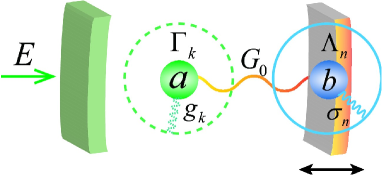
Figure 1: A cavity optomechanical system driven by a monochromatic laser. The optical and mechanical modes are coupled via radiation pressure while independently coupled to their respective reservoirs.

We first construct an open-quantum-system description of a cavity optomechanical system in the coherent-state representation as shown in Fig. 1. The Fabry-Pérot cavity, known as the simplest optical resonator structure, is additionally driven by a monochromatic laser, described by the radiation-pressure interaction between an optical cavity field and a vibrating end mirror, which applies to a wide variety of optomechanical devices, including microwave resonators ref-43 , optomechanical crystals ref-44 , and setups with the membrane inside a cavity ref-45 .

Meanwhile, we assume that a cavity optomechanical system is coupled to two reservoirs. The optical mode is coupled to a reservoir characterized by zero-temperature electromagnetic modes, while the mechanical mode is coupled to another reservoir consisting of harmonic oscillators at thermal equilibrium ref-46 . In the Heisenberg picture, the system and environment evolve in time under the influence of the total Hamiltonian that reads

$${H_{\rm{T}}}={H_{\rm{S}}}+{H_{\rm{B}}},$$ (1)

where

$${H_{\rm{S}}}\!\! = \!\!+\hbar{\Delta_{0}}{a^{\dagger}}a+\hbar{\omega_{\rm{m}}}{b^{\dagger}}b-\hbar\frac{{{G_{0}}}}{{\sqrt{2}}}{a^{\dagger}}a\left({{b^{\dagger}}+b}\right)$$ (2)

$$+i\hbar\left({E{a^{\dagger}}-{E^{*}}a}\right),$$

$${H_{\rm{E}}}\!\! = \!\!+\hbar\sum\limits_{k}{{\omega_{k}}\Gamma_{k}^{\dagger}}{\Gamma_{k}}+\hbar\sum\limits_{k}{{g_{k}}\left({\Gamma_{k}^{\dagger}a+{a^{\dagger}}{\Gamma_{k}}}\right)}$$

$$+\hbar\sum\limits_{n}{{\omega_{n}}\Lambda_{n}^{\dagger}}{\Lambda_{n}}-i\hbar\sum\limits_{n}{\frac{{{\sigma_{n}}}}{2}\left({\Lambda_{n}^{\dagger}-{\Lambda_{n}}}\right)}\left({{b^{\dagger}}+b}\right),$$

with ${a^{\dagger}}$ $\left(a\right)$ denoting ${b^{\dagger}}$ $\left(b\right)$ are the creation (annihilation) operators of the optical mode and the mechanical mode, respectively. Laser detuning from the cavity resonance is ${\Delta_{0}}={\omega_{\rm{c}}}-{\omega_{L}}$, where ${\omega_{\rm{c}}}$ is the cavity characteristic frequency and ${\omega_{L}}$ the is driving laser frequency. The characteristic frequency and effective mass of the mechanical oscillator are ${\omega_{\rm{m}}}$ and $m$, respectively. The optomechanical coupling coefficient is ${G_{0}}=\left({{{{\omega_{\rm{c}}}}\mathord{/{\vphantom{{{\omega_{\rm{c}}}}L}}\kern-1.2pt}L}}\right)\sqrt{{\hbar\mathord{/{\vphantom{\hbar{m{\omega_{\rm{m}}}}}}\kern-1.2pt}{m{\omega_{\rm{m}}}}}}$, with $L$ being the cavity length. The complex amplitude of the driving laser is $E$. In addition, $\Gamma_{k}^{\dagger}$ $\left({{\Gamma_{k}}}\right)$ and $\Lambda_{n}^{\dagger}$ $\left({{\Lambda_{n}}}\right)$ for ${k}\in\left\{{1,2,3\cdot\cdot\cdot,+\infty}\right\}$ and ${n}\in\left\{{1,2,3\cdot\cdot\cdot,+\infty}\right\}$ are, respectively, the creation (annihilation) operators of the reservoirs for the optical mode and the mechanical mode. The harmonic-oscillator reservoirs have closely spaced frequencies corresponding to photons and phonons, denoted by ${\omega_{k}}$ and ${{\omega_{n}}}$, respectively. The real numbers ${g_{k}}$ and ${\sigma_{n}}$ represent the coupling strengths between the subsystem and the $n$th reservoir mode, respectively. Details of the derivations of the total Hamiltonian (1) are attached in Appendix A ref-47 .

II.2 Nonlinear Langevin equations

A reasonable description of the dynamics in an open quantum system should include photon losses in the optical cavity field and the Brownian noise acting on the vibrating end mirror. By substituting Eq. (1) into the Heisenberg equation and taking into account the dissipation and noise terms, we obtain a set of closed integrodifferential equations (see Appendix B for the derivation ref-47 ) for the operators of the optical mode and mechanical mode as follows:

$$\dot{q} = {\omega_{\rm{m}}}p,$$ (4)

$$\dot{p} = -{\omega_{\rm{m}}}q-{\gamma_{\rm{m}}}p+{G_{0}}{a^{\dagger}}a+\xi,$$ (5)

$$\dot{a} = -\left({\kappa+i{\Delta_{0}}}\right)a+i{G_{0}}aq+E+\sqrt{2\kappa}{a_{{\rm{in}}}},$$ (6)

where $q={{\left({{b^{\dagger}}+b}\right)}\mathord{/{\vphantom{{\left({{b^{\dagger}}+b}\right)}{\sqrt{2}}}}\kern-1.2pt}{\sqrt{2}}}$ and $p={{i\left({{b^{\dagger}}-b}\right)}\mathord{/{\vphantom{{i\left({{b^{\dagger}}-b}\right)}{\sqrt{2}}}}\kern-1.2pt}{\sqrt{2}}}$ are the dimensionless position and momentum operators of the vibrating end mirror. We assume that the decay rate of the optical cavity is $\kappa$ and set the mechanical damping rate as ${\gamma_{\rm{m}}}={\omega_{\rm{m}}}\gamma$. The dissipative terms $\kappa$ and $\gamma$ are proportional to the square of the coupling strength between the subsystem and the reservoir ${g_{k}}$ and ${\sigma_{n}}$, respectively. The optical Langevin force ${a_{{\rm{in}}}}$ represents the field incident to the cavity and is assumed to be in the vacuum state. Its specific expression and the correlation function ref-48 are

$${a_{{\rm{in}}}}\left(t\right)\! = \!\frac{{-i}}{{\sqrt{2\pi}}}\sum\limits_{k}{{g_{k}}}\Gamma\left({{t_{0}}}\right){e^{-i{\omega_{k}}\left({t-{t_{0}}}\right)}},$$

$$\langle{{a_{{\rm{in}}}}\left(t\right)a_{{\rm{in}}}^{\dagger}\left({t^{\prime}}\right)}\rangle\! = \!\delta\left({t-t^{\prime}}\right),$$ (7)

where ${t_{0}}$ represents the initial time. This correlation function is true for optical fields at room temperature or microwaves at a cryostat.

In contrast, the Brownian noise operator is given by

$$\xi\left(t\right)\!=\!\sum\limits_{n}\!{\frac{{i{\sigma_{n}}}}{{\sqrt{2}}}}\!\left[{\Lambda_{n}^{\dagger}\left({{t_{0}}}\right){e^{i{\omega_{n}}\left({t-{t_{0}}}\right)}}\!-\!{\Lambda_{n}}\left({{t_{0}}}\right){e^{-i{\omega_{n}}\left({t-{t_{0}}}\right)}}}\right],$$ (8)

The mechanical damping force $\xi$ is non-Markovian in general ref-49 , but it can be treated as Markovian if the following two conditions are met: the thermal bath occupation number satisfies ${{\bar{n}}}\gg{\rm{1}}$; the mechanical quality factor satisfies $Q={{{\omega_{\rm{m}}}}\mathord{\left/{\vphantom{{{\omega_{\rm{m}}}}{{\gamma_{\rm{m}}}={1\mathord{\left/{\vphantom{1\gamma}}\right.\kern-1.2pt}\gamma}}}}\right.\kern-1.2pt}{{\gamma_{\rm{m}}}={1\mathord{\left/{\vphantom{1\gamma}}\right.\kern-1.2pt}\gamma}}}\gg 1$. These conditions are well satisfied in the majority of contemporary experimental setups, which validates the use of the standard Markovian delta-correlation ref-50 ; ref-51 :

$${{\left\langle{\xi\left(t\right)\xi\left({t^{\prime}}\right)+\xi\left({t^{\prime}}\right)\xi\left(t\right)}\right\rangle}\mathord{/{\vphantom{{\left\langle{\xi\left(t\right)\xi\left({t^{\prime}}\right)+\xi\left(t\right)\xi\left({t^{\prime}}\right)}\right\rangle}2}}\kern-1.2pt}2}\approx{\gamma_{\rm{m}}}\left({2{\bar{n}}+1}\right)\delta\left({t-t^{\prime}}\right),$$ (9)

where ${{\bar{n}}}={\left[{\exp\left({{{\hbar{\omega_{\rm{m}}}}\mathord{\left/{\vphantom{{\hbar{\omega_{\rm{m}}}}{{k_{\rm{B}}}T}}}\right.\kern-1.2pt}{{k_{\rm{B}}}T}}}\right)-1}\right]^{-1}}$ is the mean thermal excitation number with the Boltzmann constant ${k_{\rm{B}}}$ and the end-mirror temperature $T$.

So far, we have constructed the total Hamiltonian of the optomechanical system under the coherent-state representation and completely reproduced the results of the nonlinear Langevin equations in Ref. ref-24 , which provides solid support for the filtering model dominated by the resonance effect discussed later. We stress that deriving the Langevin equation from the total Hamiltonian provides a clear picture in explicitly revealing the specific form of the interaction between the system and the environment and the physical origin of each term in nonlinear Langevin equations, in comparison to the implicit treatment of such interactions in the Lindblad master equation.

III Resonance-dominant optomechanical entanglement

III.1 Filtering Model

In the preceding section, the Hamiltonian (1) describes an original interaction between an optomechanical system and its surrounding environment. This section proposes a resonant filtering model in the weak coupling limit between the system and the heat bath. It uses a high-frequency resonance between the mechanical mode and its thermal reservoirs to filter out non-resonant degrees of freedom and achieve quantum coherence protection.

To discuss the frequency relation between the mechanical mode and its thermal reservoirs, we introduce the frequency transformation $\tilde{b}\left(t\right)=b\left(t\right)\exp\left({i{\omega_{\rm{m}}}t}\right)$ and ${\tilde{\Lambda}_{n}}\left(t\right)={\Lambda_{n}}\left(t\right)\exp\left({i{\omega_{n}}t}\right)$ for ${b}\left(t\right)$ and ${\Lambda_{{n}}}\left(t\right)$ ref-46 in the interaction picture. After that, the Hamiltonian (1) reads

$${H_{\rm{T}}}=\!\!\!\!\! +\hbar{\Delta_{0}}{a^{\dagger}}a+\hbar{\omega_{\rm{m}}}{b^{\dagger}}b+i\hbar\left({E{a^{\dagger}}-{E^{*}}a}\right)$$

$$-\hbar\frac{{{G_{0}}}}{{\sqrt{2}}}{a^{\dagger}}a\left({{{\tilde{b}}^{\dagger}}{e^{i{\omega_{\rm{m}}}t}}+\tilde{b}{e^{-i{\omega_{\rm{m}}}t}}}\right)+\hbar\sum\limits_{k}{{\omega_{k}}\Gamma_{k}^{\dagger}}{\Gamma_{k}}$$

$$+\hbar\sum\limits_{k}{{g_{k}}\left({\Gamma_{k}^{\dagger}a+{a^{\dagger}}{\Gamma_{k}}}\right)}+\hbar\sum\limits_{n}{{\omega_{n}}\Lambda_{n}^{\dagger}}{\Lambda_{n}}$$

$$-i\hbar\sum\limits_{n}{\frac{{{\sigma_{n}}}}{2}\left[{\tilde{\Lambda}_{n}^{\dagger}\tilde{b}{e^{i\left({{\omega_{n}}-{\omega_{\rm{m}}}}\right)t}}-{{\tilde{b}}^{\dagger}}{{\tilde{\Lambda}}_{n}}{e^{-i\left({{\omega_{n}}-{\omega_{\rm{m}}}}\right)t}}}\right]}$$

$$-i\hbar\sum\limits_{n}{\frac{{{\sigma_{n}}}}{2}}\left[{\tilde{\Lambda}_{n}^{\dagger}{{\tilde{b}}^{\dagger}}{e^{i\left({{\omega_{n}}+{\omega_{\rm{m}}}}\right)t}}-\tilde{b}{{\tilde{\Lambda}}_{n}}{e^{-i\left({{\omega_{n}}+{\omega_{\rm{m}}}}\right)t}}}\right].$$

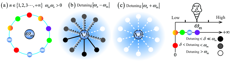
Figure 2: Schematic diagram of the filtering model. $\left({\rm{a}}\right)$ The coupling between a high-frequency mechanical oscillator and co-directional thermal reservoirs. The frequency of the thermal reservoirs sequentially transits from zero to positive infinity in rainbow color order. In $\left({\rm{b}}\right)$, the terms of $\tilde{\Lambda}_{{n}}^{\dagger}\tilde{b}$ and ${{\tilde{b}}^{\dagger}}{{\tilde{\Lambda}}_{{n}}}$ show the high-frequency resonance effect, while in $\left({\rm{c}}\right)$, the terms of $\tilde{\Lambda}_{{n}}^{\dagger}{{\tilde{b}}^{\dagger}}$ and $\tilde{b}{{\tilde{\Lambda}}_{{n}}}$ exhibit large detuning effects. The black, gray, and white colors correspond to the high-frequency resonance, moderately detuned, and highly detuned modes of the heat bath compared to the frequency of the single-mode mechanical oscillator ${\omega_{\rm{m}}}$. The parameters $\delta$ and ${\omega_{\rm{m}}}$ can be modulated by coherent laser driving ref-53 ; ref-54 .

As aforementioned, our physical model describes a Markovian process in the weak coupling limit $\gamma\ll 1$, which corresponds to Eq. (III.1) satisfying the weak-coupling limit ${\sigma_{{n}}}\ll 1$ for ${{n}}\in\left\{{1,2,3\cdot\cdot\cdot,+\infty}\right\}$ ref-52 . See Fig. 2 for a schematic diagram, according to the rotating-wave approximation, we eliminate the fast-oscillating terms from Eq. (III.1), and then recovering $b\left(t\right)=\tilde{b}\left(t\right){e^{-i{\omega_{\rm{m}}}t}}$ and ${\Lambda_{{n}}}\left(t\right)={{\tilde{\Lambda}}_{{n}}}\left(t\right){e^{-i{\omega_{{n}}}t}}$, we classify the filtering model reduced from Eq. (III.1) as follows.

The high-frequency resonance region is defined by ${\omega_{\rm{m}}}{\omega_{{n}}}>0$ and ${\omega_{{n}}}\in\left({0,+\infty}\right)$. We here propose to filter out the strongly non-resonant contributions ${\tilde{\Lambda}_{{n}}^{\dagger}{{\tilde{b}}^{\dagger}}}$ and ${\tilde{b}{{\tilde{\Lambda}}_{{n}}}}$ mechanically; see Sec. III-D for possible experimental realizations. Keeping only the resonant terms ${\tilde{\Lambda}_{{n}}^{\dagger}\tilde{b}}$ and ${{{\tilde{b}}^{\dagger}}{{\tilde{\Lambda}}_{{n}}}}$, the filtering model is

$${H_{\rm{F}}}=\!\!\!\!\! +\hbar{\Delta_{0}}{a^{\dagger}}a+\hbar{\omega_{\rm{m}}}{b^{\dagger}}b+i\hbar\left({E{a^{\dagger}}-{E^{*}}a}\right)$$ (11)

$$-\hbar\frac{{{G_{0}}}}{{\sqrt{2}}}{a^{\dagger}}a\left({b+{b^{\dagger}}}\right)+\hbar\sum\limits_{k}{{\omega_{k}}\Gamma_{k}^{\dagger}}{\Gamma_{k}}$$

$$+\hbar\sum\limits_{k}{{g_{k}}\left({\Gamma_{k}^{\dagger}a+{a^{\dagger}}{\Gamma_{k}}}\right)}+\hbar\sum\limits_{n}{{\omega_{n}}\Lambda_{n}^{\dagger}}{\Lambda_{n}}$$

$$-i\hbar\sum\limits_{n}{\frac{{{\sigma_{n}}}}{2}\left[{\Lambda_{n}^{\dagger}b-{b^{\dagger}}{\Lambda_{n}}}\right]}.$$

The resonance terms ${\tilde{\Lambda}_{{n}}^{\dagger}\tilde{b}}$ and ${{{\tilde{b}}^{\dagger}}{{\tilde{\Lambda}}_{{n}}}}$ in this region describe the exchange of quanta between the mechanical mode and its $n$th thermal reservoir mode ref-18 . In contrast, the high-frequency inverse-resonance region is defined by ${\omega_{\rm{m}}}{\omega_{n}}<0$ and ${\omega_{{n}}}\in\left({0,-\infty}\right)$. Keeping only the terms of ${\tilde{\Lambda}_{{n}}^{\dagger}{{\tilde{b}}^{\dagger}}}$ and ${\tilde{b}{{\tilde{\Lambda}}_{{n}}}}$, the inverse-filtering model reads

$$H_{\rm{F}}^{\rm{I}}=\!\!\!\!\! +\hbar{\Delta_{0}}{a^{\dagger}}a+\hbar{\omega_{\rm{m}}}{b^{\dagger}}b+i\hbar\left({E{a^{\dagger}}-{E^{*}}a}\right)$$ (12)

$$-\hbar\frac{{{G_{0}}}}{{\sqrt{2}}}{a^{\dagger}}a\left({b+{b^{\dagger}}}\right)+\hbar\sum\limits_{k}{{\omega_{k}}\Gamma_{k}^{\dagger}}{\Gamma_{k}}$$

$$+\hbar\sum\limits_{k}{{g_{k}}\left({\Gamma_{k}^{\dagger}a+{a^{\dagger}}{\Gamma_{k}}}\right)}+\hbar\sum\limits_{n}{{\omega_{n}}\Lambda_{n}^{\dagger}}{\Lambda_{n}}$$

$$-i\hbar\sum\limits_{n}{\frac{{{\sigma_{n}}}}{2}\left[{\Lambda_{n}^{\dagger}{b^{\dagger}}-b{\Lambda_{n}}}\right]}.$$

The inverse-resonance terms ${\tilde{\Lambda}_{{n}}^{\dagger}{{\tilde{b}}^{\dagger}}}$ and ${\tilde{b}{{\tilde{\Lambda}}_{{n}}}}$ in this region represent a two-mode squeezing interaction between the mechanical mode and its $n$th thermal reservoir mode, and the parametric amplification relies on the two-mode squeezing interaction ref-55 .

III.2 The Lyapunov equation for the steady-state correlation matrix

In order to comprehend the impact of resonance effects between a mechanical mode and its thermal reservoirs on the strength of an optomechanical system, it is crucial to gain insight into the structure of optomechanical correlation in open quantum systems. For this purpose, we use the Lyapunov equation to compute the steady-state correlation matrix between subsystems and obtain the optomechanical entanglement strength ref-56 . Without loss of generality, we take the high-frequency resonance regime as an example of deriving the Lyapunov equation in terms of the steady-state correlation matrix.

By deriving the Heisenberg equation of motion of the resonant Hamiltonian ${H_{\rm{F}}}$ (11), we obtain nonlinear Langevin equations that govern the dynamical behavior of the optomechanical system in the high-frequency resonance regime. The nonlinear Langevin equations are written as (see Appendix C for details)

$$\dot{q} = {\omega_{\rm{m}}}p+\frac{\gamma}{4}\dot{p}+\frac{1}{2}\xi^{\prime},$$ (13)

$$\dot{p} = -{\omega_{\rm{m}}}q-\frac{\gamma}{4}\dot{q}+{G_{0}}{a^{\dagger}}a+\frac{1}{2}\xi,$$ (14)

$$\dot{a} = -\left({\kappa+i{\Delta_{0}}}\right)a+i{G_{0}}aq+E+\sqrt{2\kappa}{a_{{\rm{in}}}},$$ (15)

where the Brownian noise operator reads

$$\xi^{\prime}\!\left(t\right)\!=\!\!\sum\limits_{n}\!{\frac{{{\sigma_{n}}}}{{\sqrt{2}}}}\!\!\left[{\Lambda_{n}^{\dagger}\left({{t_{0}}}\right){e^{i{\omega_{n}}\left({t-{t_{0}}}\right)}}\!\!+\!{\Lambda_{n}}\left({{t_{0}}}\right){e^{-i{\omega_{n}}\left({t-{t_{0}}}\right)}}}\right]\!\!.$$ (16)

In the weak-coupling limit $\gamma\ll 1$, by substituting Eqs. (13) and (14) into each other and neglecting small terms in Eqs. (13)-(14), we obtain the reduced equations

$$\dot{q} = {\omega_{\rm{m}}}p-\frac{{{\gamma_{\rm{m}}}}}{4}q+\frac{1}{2}\xi^{\prime}$$ (17)

$$\dot{p} = -{\omega_{\rm{m}}}q-\frac{{{\gamma_{\rm{m}}}}}{4}p+{G_{0}}{a^{\dagger}}a+\frac{1}{2}\xi.$$ (18)

In the weak-coupling limit $\gamma\ll 1$, the Brownian noise operator $\xi^{\prime}\left(t\right)$ has the same delta-correlated form as $\xi\left(t\right)$.

The nonlinear Langevin equations (15), (17) and (18) are inherently nonlinear as they contain a product of the photon operator and dimensionless position operator of the mechanical phonon, $aq$, as well as a quadratic term in photon operators, ${a^{\dagger}}a$. Using the standard mean-field method ref-57 to solve Eqs. (15), (17) and (18), we start by splitting each Heisenberg operator into the classical mean values and quantum fluctuation operators, i.e., $a={\alpha_{\rm{s}}}+\delta a$ as in ${a^{\dagger}}=\alpha_{\rm{s}}^{*}+\delta{a^{\dagger}}$, $q={q_{\rm{s}}}+\delta q$, and $p={p_{\rm{s}}}+\delta p$, thereby linearizing these equations. Adopting the above approach and inserting these expressions into nonlinear Langevin equations (15), (17) and (18), we find the solution of the mean values for the classical steady state given by ${p_{\rm{s}}}={{\gamma{q_{\rm{s}}}}\mathord{/{\vphantom{{\gamma{q_{\rm{s}}}}4}}\kern-1.2pt}4}\approx 0$, ${q_{\rm{s}}}={{{G_{0}}\alpha_{\rm{s}}^{*}{\alpha_{\rm{s}}}}\mathord{/{\vphantom{{{G_{0}}\alpha_{\rm{s}}^{*}{\alpha_{\rm{s}}}}{{\omega_{\rm{m}}}}}}\kern-1.2pt}{{\omega_{\rm{m}}}}}$, and ${\alpha_{\rm{s}}}={E\mathord{/{\vphantom{E{\left({\kappa+i\Delta}\right)}}}\kern-1.2pt}{\left({\kappa+i\Delta}\right)}}$, where we set normalization of the detuning frequency of the optical field as $\Delta={\Delta_{0}}-{{G_{0}^{2}\alpha_{\rm{s}}^{*}{\alpha_{\rm{s}}}}\mathord{/{\vphantom{{iG_{0}^{2}\alpha_{\rm{s}}^{*}{\alpha_{\rm{s}}}}{{\omega_{\rm{m}}}}}}\kern-1.2pt}{{\omega_{\rm{m}}}}}{\rm{}}$. The parameter regime for generating optomechanical entanglement is the one with a large amplitude of the driving laser $E$, i.e., ${\alpha_{\rm{s}}}\gg\delta a$ and $\alpha_{\rm{s}}^{*}\gg\delta{a^{\dagger}}$. By dropping the contribution of terms of second orders in quantum fluctuations $\delta a\delta q$ and $\delta{a^{\dagger}}\delta a$, we obtain the linearized Langevin equations

$$\delta\dot{q}\! = \!{\omega_{\rm{m}}}\delta p-\frac{{{\gamma_{\rm{m}}}}}{4}\delta q+\frac{1}{2}\xi^{\prime},$$ (19)

$$\delta\dot{p}\! = \!-{\omega_{\rm{m}}}\delta q-\frac{{{\gamma_{\rm{m}}}}}{4}\delta p+{G_{0}}\left({\alpha_{\rm{s}}^{*}\delta a+{\alpha_{\rm{s}}}\delta{a^{\dagger}}}\right)+\frac{1}{2}\xi,$$ (20)

$$\delta\dot{a}\! = \!-\left({\kappa+i\Delta}\right)\delta a+i{G_{0}}{\alpha_{\rm{s}}}\delta q+\sqrt{2\kappa}{a_{{\rm{in}}}}.$$ (21)

By assuming the driving laser amplitude $E=\left|E\right|\exp\left({i\varphi}\right)$, where $\left|E\right|$ is related to the input laser power $P$ by $\left|E\right|=\sqrt{{{2P\kappa}\mathord{\left/{\vphantom{{2P\kappa}{\hbar{\omega_{L}}}}}\right.\kern-1.2pt}{\hbar{\omega_{L}}}}}$ and $\varphi$ denotes the phase of the laser field coupling to the optical cavity field, we choose $\varphi$ to satisfy $\tan\left(\varphi\right)={\Delta\mathord{/{\vphantom{\Delta\kappa}}\kern-1.2pt}\kappa}$ so that ${{\alpha_{\rm{s}}}}$ may be real.

The quadratures play an essential role in studying entanglement because they are used to quantify the correlations between different modes. We define the cavity field quadratures $\delta X={{\left({\delta a+\delta{a^{\dagger}}}\right)}\mathord{/{\vphantom{{\left({\delta a+\delta{a^{\dagger}}}\right)}{\sqrt{2}}}}\kern-1.2pt}{\sqrt{2}}}$ and $\delta Y=i{{\left({\delta{a^{\dagger}}-\delta a}\right)}\mathord{/{\vphantom{{\left({\delta{a^{\dagger}}-\delta a}\right)}{\sqrt{2}}}}\kern-1.2pt}{\sqrt{2}}}$ as two observables that describe the quantum state of a cavity field mode, which can be measured using homodyne detection techniques. Accordingly, we define the orthogonal input noise operators ${X_{{\rm{in}}}}={{({\delta a_{{\rm{in}}}^{\dagger}+\delta{a_{{\rm{in}}}}})}\mathord{/{\vphantom{{\left({\delta a_{{\rm{in}}}^{\dagger}+\delta{a_{{\rm{in}}}}}\right)}{\sqrt{2}}}}\kern-1.2pt}{\sqrt{2}}}$ and ${Y_{{\rm{in}}}}=i{{({\delta a_{{\rm{in}}}^{\dagger}-\delta{a_{{\rm{in}}}}})}\mathord{/{\vphantom{{\left({\delta a_{{\rm{in}}}^{\dagger}-\delta{a_{{\rm{in}}}}}\right)}{\sqrt{2}}}}\kern-1.2pt}{\sqrt{2}}}$, and thereby rewrite Eqs. (19)-(21) as

$$\delta\dot{q} = {\omega_{\rm{m}}}\delta p-\frac{{{\gamma_{\rm{m}}}}}{4}\delta q+\frac{1}{2}\xi^{\prime},$$ (22)

$$\delta\dot{p} = -{\omega_{\rm{m}}}\delta q-\frac{{{\gamma_{\rm{m}}}}}{4}\delta p+G\delta X+\frac{1}{2}\xi,$$ (23)

$$\delta\dot{X} = -{\kappa}\delta X+\Delta\delta Y+\sqrt{2{\kappa}}{X_{{\rm{in}}}},$$ (24)

$$\delta\dot{Y} = -{\kappa}\delta Y-\Delta\delta X+G\delta q+\sqrt{2{\kappa}}Y_{{\rm{in}}},$$ (25)

where the effective optomechanical coupling is given by $G=\sqrt{2}{\alpha_{\rm{s}}}{G_{0}}$.

For convenience, we concisely express a linearized Langevin Eqs. (22)-(25) for orthogonal operators in a matrix form,

$$\dot{\mu}\left(t\right)={{A}}\mu\left(t\right)+n\left(t\right),$$ (26)

where the component of each matrix is as follows: the transposes of the column vector of continuous variables fluctuation operators are written as ${\mu^{T}}\left(t\right)=\left[{\delta q\left(t\right),\delta p\left(t\right),\delta X\left(t\right),\delta Y\left(t\right)}\right]$; the transposes of the column vector of noise operators are denoted by ${n^{T}}\left(t\right)=\left[{0.5\xi^{\prime}\left(t\right),0.5\xi\left(t\right),\sqrt{2\kappa}{X_{{\rm{in}}}}\left(t\right),\sqrt{2\kappa}{Y_{{\rm{in}}}}\left(t\right)}\right]$; the coefficient matrix ${{A}}$ in terms of system parameters takes the form

$${{A}}=\left({\begin{array}[]{*{20}{c}}{-0.25{\gamma_{\rm{m}}}}&{{\omega_{\rm{m}}}}&0&0\\ {-{\omega_{\rm{m}}}}&{-0.25{\gamma_{\rm{m}}}}&G&0\\ 0&0&{-\kappa}&\Delta\\ G&0&{-\Delta}&{-\kappa}\end{array}}\right).$$ (31)

The solution of Eq. (26) can be expressed as

$$\mu\left(t\right)={{M}}\left(t\right)\mu\left({t_{0}}\right)+\int_{t_{0}}^{t}{{{M}}\left(\tau\right)}n\left({t-\tau}\right)d\tau,$$ (32)

where ${M}$ is the matrix exponential ${{M}}\left(t\right)=\exp\left({{\rm{A}}t}\right)$ and we assume the initial time as ${t_{0}}=0$. The system is stable if and only if the real parts of all the eigenvalues of the matrix ${{A}}$ are negative. The eigenvalue equation det$\left|{{{A}}-\lambda{{\rm{I}}_{4}}}\right|=[{{{\left({0.25{\gamma_{\rm{m}}}+\lambda}\right)}^{2}}+\omega_{\rm{m}}^{2}}][{{{\left({\kappa+\lambda}\right)}^{2}}+{\Delta^{2}}}]-{\omega_{\rm{m}}}{G^{2}}\Delta=0$, where ${{{\rm{I}}_{4}}}$ denotes the four-dimensional identity matrix, can be reduced to the fourth-order equation ${C_{0}}{\lambda^{4}}+{C_{1}}{\lambda^{3}}+{C_{2}}{\lambda^{2}}+{C_{3}}\lambda+{C_{4}}{\rm{=}}0$. The stability conditions can be derived by applying the Routh-Hurwitz criterion ref-58 as follows: ​​​${C_{0}}>\!\!0,\ {C_{1}}>0,\ {C_{1}}{C_{2}}-{C_{0}}{C_{3}}>0,\ \left({{C_{1}}{C_{2}}-{C_{0}}{C_{3}}}\right){C_{3}}-C_{1}^{2}{C_{4}}>0,\ {C_{4}}>0$, yielding the following two nontrivial conditions: $\left({\omega_{\rm{m}}^{2}+{{\gamma_{\rm{m}}^{2}}\mathord{\left/{\vphantom{{\gamma_{\rm{m}}^{2}}{16}}}\right.\kern-1.2pt}{16}}}\right)\left({{\Delta^{2}}+{\kappa^{2}}}\right)-{\omega_{\rm{m}}}{G^{2}}\Delta>0$ and

$$+{\gamma_{\rm{m}}}\kappa\left\{{{\Delta^{4}}+{\Delta^{2}}\left({\frac{{\gamma_{\rm{m}}^{2}}}{8}+{\gamma_{\rm{m}}}\kappa+2{\kappa^{2}}-2\omega_{\rm{m}}^{2}}\right)+\frac{1}{{256}}{{\left[{16\omega_{\rm{m}}^{2}+{{\left({{\gamma_{\rm{m}}}+4\kappa}\right)}^{2}}}\right]}^{2}}}\right\}+{\omega_{\rm{m}}}{G^{2}}\Delta{\left({\frac{{{\gamma_{\rm{m}}}}}{2}+2\kappa}\right)^{2}}>0.$$ (33)

The following numerical simulation shows that realistic experimental parameter configurations always meet these stability conditions. When the system is stable, it reaches a unique steady state in the long-time limit $t\to+\infty$ independently of the initial condition.

We set the initial to a Gaussian state, and the linear dynamics preserve the noise operators ${\xi^{\prime}}$, $\xi$, and ${a_{{\rm{in}}}}$. Thus, the correlation properties of the system can be completely characterized by its two first moments, of which we are interested in the second one, namely the covariance matrix with elements defined as

$${{{V}}_{{{ij}}}}\! = \!\frac{1}{2}\left\langle{{\mu_{{i}}}\left({+\infty}\right){\mu_{{j}}}\left({+\infty}\right)+{\mu_{{j}}}\left({+\infty}\right){\mu_{{i}}}\left({+\infty}\right)}\right\rangle$$

$$= \sum\limits_{{{k}},{{l}}}{\int_{{t_{0}}}^{+\infty}\!{d\tau\int_{{t_{0}}}^{+\infty}\!{d\tau^{\prime}{{{M}}_{{{ik}}}}\left(\tau\right)}}}{{{M}}_{{{jl}}}}\left({\tau^{\prime}}\right){\Phi_{{{kl}}}}\left({\tau-\tau^{\prime}}\right),$$

where ${\Phi_{{{kl}}}}\left({\tau-\tau^{\prime}}\right)={{\left\langle{{n_{{k}}}\left(\tau\right){n_{{l}}}\left({\tau^{\prime}}\right)+{n_{{l}}}\left({\tau^{\prime}}\right){n_{{k}}}\left(\tau\right)}\right\rangle}\mathord{\left/{\vphantom{{\left\langle{{n_{{k}}}\left(\tau\right){n_{{l}}}\left({\tau^{\prime}}\right)+{n_{{l}}}\left({\tau^{\prime}}\right){n_{{k}}}\left(\tau\right)}\right\rangle}2}}\right.\kern-1.2pt}2}$ is the matrix of the stationary noise correlation functions. Because the matrix elements are independent of $n\left(t\right)$, we obtain ${\Phi_{{{kl}}}}\left({\tau-\tau^{\prime}}\right)={{{D}}_{{{kl}}}}\delta\left({\tau-\tau^{\prime}}\right)$, where ${{D}}={\rm{Diag}}\left[{{{{\gamma_{\rm{m}}}\left({2{{\bar{n}}}+1}\right)}\mathord{\left/{\vphantom{{{\gamma_{\rm{m}}}\left({2{{\bar{n}}}+1}\right)}4}}\right.\kern-1.2pt}4},{{{\gamma_{\rm{m}}}\left({2{{\bar{n}}}+1}\right)}\mathord{\left/{\vphantom{{{\gamma_{\rm{m}}}\left({2{{\bar{n}}}+1}\right)}4}}\right.\kern-1.2pt}4},\kappa,\kappa}\right]$ is a diagonal matrix. According to Eq. (III.2) and the form of ${\Phi_{{{kl}}}}\left({\tau-\tau^{\prime}}\right)$, we find that the expression of the matrix ${{V}}$ is equivalent to

$${{V}}=\int_{{t_{0}}}^{+\infty}{{{M}}\left(\tau\right){{DM}}{{\left(\tau\right)}^{T}}d\tau}.$$ (35)

Hence, we obtain

$$AV = \int_{t_{0}}^{\infty}AM(\tau)DM(\tau)^{T}d\tau$$

$$= \int_{t_{0}}^{\infty}\frac{d}{d\tau}M(\tau)DM(\tau)^{T}d\tau,$$

$$VA^{T} = \int_{t_{0}}^{\infty}M(\tau)D(AM(\tau))^{T}d\tau$$

$$= \int_{t_{0}}^{\infty}M(\tau)D\frac{d}{d\tau}M(\tau)^{T}d\tau.$$

The combination of Eqs. (III.2) and (III.2) becomes

$$AV+V{A^{T}}= \!\!\!\!+\int_{{t_{0}}}^{\infty}{\frac{d}{{d\tau}}}[M(\tau)DM{(\tau)^{T}}]d\tau$$ (38)

$$\!\!\!\!-\int_{{t_{0}}}^{\infty}M(\tau)\frac{d}{{d\tau}}DM{(\tau)^{T}}d\tau$$

$$= \!\!\!\![M\left(\tau\right)DM{{\left(\tau\right)}^{T}}]|_{{t_{0}}}^{+\infty}=-D$$

where we use the assumptions that the stability conditions are satisfied. The solution ${{M}}\left({+\infty}\right)$ converges to zero in the long-time limit. Equation (38) is a linear Lyapunov equation with respect to ${V}$, which can be solved straightforwardly. See Appendix D for a detailed derivation of a Lyapunov equation (38).

We can derive a Lyapunov equation satisfied by the high-frequency inverse-resonance Hamiltonian $H_{{\rm{F}}}^{{\rm{I}}}$ in Eq. (12) similarly to the form of the high-frequency resonance Hamiltonian $H_{{\rm{F}}}$ in Eq. (11). Moreover, we show that the analysis and results concerning optomechanical entanglement in the high-frequency inverse-resonance regime are equivalent to those in the high-frequency resonance regime. Therefore, we do not elaborate on it further here.

III.3 Optomechanical entanglement

Cavity optomechanical systems naturally exhibit complex entanglement structures and always involve mixed states and continuous variable entanglement, which are affected by dissipation and noise. In this sense, the logarithmic negativity is a powerful tool that can provide valuable insights into the nature of optomechanical entanglement ref-59 , which can be experimentally measured using homodyne detection. Thus, we use the logarithmic negativity ${E_{\rm{N}}}$ to measure optomechanical entanglement between the optical cavity field and the mechanical oscillator. It provides an obvious easy way to compute an upper bound for the distillable optomechanical entanglement ref-60 .

As mentioned in the continuous variable scenario, the bipartite optomechanical entanglement can be quantified as ref-56

$${E_{\rm{N}}}=\max\left[{0,-\ln\left({2{\Xi}}\right)}\right],$$ (39)

where

$$\Xi=\frac{1}{{\sqrt{2}}}{\left\{{\Sigma\left({{V}}\right)-\sqrt{{{\left[{\Sigma\left({{V}}\right)}\right]}^{2}}-4\det\left({{V}}\right)}}\right\}^{\frac{1}{2}}}$$ (40)

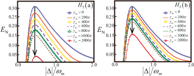
Figure 3: Plot of the logarithmic negativity ${E_{\rm{N}}}$ as a function of the normalized detuning frequency of the optical field $\left|\Delta\right|$ (in units of ${{\omega_{\rm{m}}}}$) for seven values of the mechanical damping rate: ${\gamma_{\rm{m}}}=0$ (blue circular line), ${\gamma_{\rm{m}}}=200\pi{\rm{Hz}}$ (orange solid line), ${\gamma_{\rm{m}}}=400\pi{\rm{Hz}}$ (yellow square line), ${\gamma_{\rm{m}}}=600\pi{\rm{Hz}}$ (purple dashed line), ${\gamma_{\rm{m}}}=800\pi{\rm{Hz}}$ (green triangle line), ${\gamma_{\rm{m}}}=1000\pi{\rm{Hz}}$ (brown dotted line), and ${\gamma_{\rm{m}}}=2000\pi{\rm{Hz}}$ (red cross line), where $\left({\rm{a}}\right)$ and $\left({\rm{b}}\right)$ correspond to the original model ${H_{\rm{T}}}$ in Eq. (III.1) and the filtering model ${H_{{\rm{F}}}}$ in Eq. (11), respectively. The length of the black downward-pointing arrows indicates how sensitive optomechanical entanglement is to ${\gamma_{\rm{m}}}$. The other parameters for $\left({\rm{a}}\right)$ and $\left({\rm{b}}\right)$ are chosen as follows: the optical cavity of length $L=1{\rm{mm}}$ and the drives laser with wavelength $\lambda=810{\rm{nm}}$ and power $P=50{\rm{mW}}$. The decay rate of the optical cavity is chosen to be $\kappa=8.8\pi\times{10^{6}}{\rm{Hz}}$, the optical finesse $F=\pi c/L\kappa\approx 3.4\times{10^{4}}$ with $c=3\times{10^{8}}{\rm{m}}/{\rm{s}}$, and the driving laser frequency is resonant with the characteristic frequency of the cavity field, ${\omega_{L}}={\omega_{\rm{c}}}=2\pi c/\lambda$. The mechanical oscillator has the characteristic frequency ${\omega_{\rm{m}}}=20\pi{\rm{MHz}}$, the effective mass $m=50{\rm{ng}}$, and its temperature is $T=400{\rm{mK}}$ ref-24 .

is the lowest symplectic eigenvalue of the partial transpose of the $4\times 4$ steady-state correlation matrix ref-61 . For simplicity, we denote the $4\times 4$ steady-state correlation matrix as in $2\times 2$ block matrix form, which is given by ${{V}}=\left[{\left({\Theta,\beta}\right),\left({{\beta^{T}},\eta}\right)}\right]$, and $\Sigma\left({{V}}\right)=\det\left(\Theta\right)+\det\left(\eta\right)-2\det\left(\beta\right)$. We note that a Gaussian state is entangled if and only if $\Xi<{1\mathord{\left/{\vphantom{12}}\right.\kern-1.2pt}2}$. It is equivalent to Simon’s entanglement criteria for all bipartite Gaussian states ref-62 , which can be written as $4\det\left({{V}}\right)<\Sigma{\left({{V}}\right)}-{1\mathord{\left/{\vphantom{14}}\right.\kern-1.2pt}4}$.

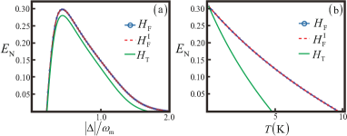
Figure 4: Comparing the optomechanical entanglement properties under different mechanisms, the high-frequency resonance of the filtering model $H_{{\rm{F}}}$ in Eq. (11) (blue circular line), the high-frequency inverse-resonance of the filtering model $H_{{\rm{F}}}^{{\rm{I}}}$ in Eq. (12) (red dashed line), and the original model ${H_{\rm{T}}}$ in Eq. (III.1) (green solid line). $\left({\rm{a}}\right)$ Plot of the logarithmic negativity ${E_{\rm{N}}}$ as a function of the normalized detuning frequency of the optical field $\left|\Delta\right|$ (in units of ${{\omega_{\rm{m}}}}$). We set ${\gamma_{\rm{m}}}=200\pi{\rm{Hz}}$ and $T=400{\rm{mK}}$. $\left({\rm{b}}\right)$ Plot of the logarithmic negativity ${E_{\rm{N}}}$ versus the mirror temperature $T$. We set ${\gamma_{\rm{m}}}=200\pi{\rm{Hz}}$ and $\Delta=0.5{\omega_{\rm{m}}}=10\pi{\rm{MHz}}$. Both in $\left({\rm{a}}\right)$ and $\left({\rm{b}}\right)$, the other parameter values are the same as in Fig. 3.

We numerically calculated the negativity for cavity optomechanical systems as shown in Figs. 3 and 4. In our numerical simulation, we utilize the parameter values identical to those outlined in Ref. ref-24 , which agree with the current optomechanical experiments configurations ref-63 ; ref-64 ; ref-65 ; ref-66 and satisfy the stability conditions (33). To begin with, we set the initial closed-optomechanical system in a maximum optomechanical entangled state. For simplicity, we assume that the driving laser frequency ${\omega_{L}}$ is resonant with the characteristic frequency ${\omega_{\rm{c}}}$ of the cavity field, that is, the laser detuning from the cavity resonance satisfies ${\Delta_{0}}=0$.

In Fig. 3, we compare the sensitivity of the optomechanical entanglement ${E_{\rm{N}}}$ to the mechanical damping rate ${\gamma_{\rm{m}}}$ for the two optomechanical systems, ${H_{\rm{T}}}$ in Eq. (III.1) and $H_{\rm{F}}$ in Eq. (11). We show a significant enhancement of the robustness of optomechanical entanglement for $H_{{\rm{F}}}$ against ${\gamma_{\rm{m}}}$. Specifically, we observe that the length of the black downward-pointing arrow in Fig. 3$\left({\rm{b}}\right)$ is approximately half of that in Fig. 3$\left({\rm{a}}\right)$, which implies that the optomechanical entanglement of the filtering model ${H_{\rm{F}}}$ (11) is almost twice as robust to ${\gamma_{\rm{m}}}$ as the original model ${H_{\rm{T}}}$ (III.1). Additionally, it is worth noting that the presence of optomechanical entanglement is only within a limited range of $\left|\Delta\right|$ around $\left|\Delta\right|\approx{\omega_{\rm{m}}}$, which means that the frequency resonance between the normalization of the detuning frequency of the optical field $\left|\Delta\right|$ and the frequency of the mechanical oscillator ${\omega_{\rm{m}}}$ plays a dominant role in the generation of optomechanical entanglement.

We further examine the impact of the resonance effect between the mechanical mode and its thermal reservoir on the properties of optomechanical entanglement. For this purpose, we set ${\gamma_{\rm{m}}}=200\pi{\rm{Hz}}$ according to the actual laboratory conditions.

Figure 4$\left({\rm{a}}\right)$ shows the logarithmic negativity ${E_{\rm{N}}}$ versus the normalized detuning frequency of the optical field $\left|\Delta\right|$ (in units of ${{\omega_{\rm{m}}}}$) for cases models, the high-frequency resonance of the filtering model $H_{{\rm{F}}}$ in Eq. (11), the high-frequency inverse-resonance of the filtering model $H_{{\rm{F}}}^{{\rm{I}}}$ in Eq. (12), and the original system ${H_{\rm{T}}}$ in Eq. (III.1). It shows that the maximum optomechanical entanglements for $H_{{\rm{F}}}$ and $H_{{\rm{F}}}^{{\rm{I}}}$ are equal to each other while that for ${H_{\rm{T}}}$ is less than it. The results indicate that the resonance effect can safeguard the maximum optomechanical entanglement by filtering out the contributions from a largely detuned part of the degree of freedom, ultimately reducing both the Brownian noise $\xi$ $\left({\xi^{\prime}}\right)$ and the mechanical dissipation ${\gamma_{\rm{m}}}$.

The robustness of such an entanglement ${E_{\rm{N}}}$ with respect to the environmental temperature $T$ of the mirror is shown in Fig. 4$\left({\rm{b}}\right)$. We find that the optomechanical entanglement of the filtering model ${H_{\rm{F}}}$ in Eq. (11) remains even at temperatures around 10K and is twice the magnitude of the persistent temperature in the original model ${H_{\rm{T}}}$ in Eq. (III.1). In addition, we observe that the high-frequency resonance and the high-frequency inverse-resonance regimes have completely equivalent effects on optomechanical entanglement.

In summary, we have discussed the impact of the high-frequency resonance effect between the mechanical oscillator and its thermal reservoir on optomechanical entanglement. We have found that the resonance effect doubles the robustness of optomechanical entanglement to the mechanical dissipation and the mirror temperature. We have achieved the maximum protection of optomechanical entanglement by constructing a filtering model using resonance effects. We have observed numerically that both the high-frequency resonance and the high-frequency inverse-resonance regimes have equivalent effects on optomechanical entanglement.

III.4 Experimental Implementation

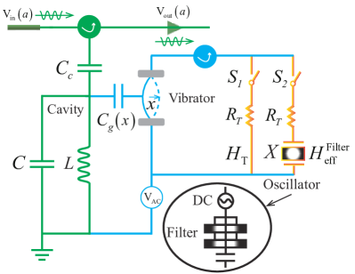
Figure 5: A circuit consisting of a resistor, inductor, and capacitor can be used to build an oscillatory filtering model for high-frequency resonance. This experimental setup comprises an on-chip optical cavity (green) coupled with a high-quality-factor nano-mechanical resonator. By turning on switch 1 and turning off switch 2, the thermistor (orange) will provide a thermal environment that couples with the resonator, corresponding to the original model ${H_{\rm{T}}}$ in Eq. (III.1). Conversely, the thermistor and the oscillator (black) will generate a high-frequency oscillation thermal environment that couples with the resonator, corresponding to the filtering model $H_{{\rm{F}}}$ in Eq. (11) Direct current, abbreviated as DC, is used for signal frequency readout.

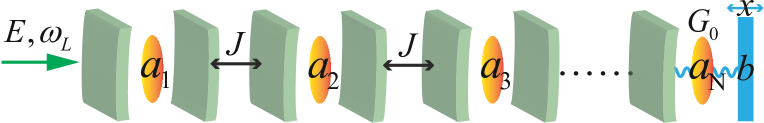
Figure 6: The schematic diagram depicts a one-dimensional array of optical cavities coupled via linear hopping between each cavity, with an oscillating end-mirror.

We propose materializing the present theoretical filtering model in a resistor-inductor-capacitor circuit ref-67 ; ref-68 ; ref-69 or superconducting quantum interference device experiments ref-70 . As shown in Fig. 5, we build an oscillatory circuit consisting of a capacitor $C$, an inductor $L$, a thermistor ${R_{T}}$, and an oscillator $X$. We set the normalized detuning frequency of the optical field of the LC circuit to satisfy $\left|\Delta\right|={1\mathord{/{\vphantom{1{({2\pi\sqrt{LC}})}}}\kern-1.2pt}{({2\pi\sqrt{LC}})}}=20\pi{\rm{MHz}}$. First, the mechanical resonator (blue) and the optical cavity (green) are connected via an inductor. Second, an extensive AC voltage bias ${{\rm{V}}_{{\rm{AC}}}}$ is applied in order to excite the mechanical resonator, represented as a movable capacitance ${C_{g}}\left(x\right)$. Here, to obtain the maximum optomechanical entanglement, the frequency of the applied voltage should be close to $\left|\Delta\right|$, namely $\left|\Delta\right|\approx{\omega_{\rm{m}}}$. Next, as the LC circuit oscillates, a current is induced in the thermistor, generating a temperature change due to the Joule heating effect. Therefore, by turning on switch 1 and turning off switch 2 simultaneously, the mechanical resonator will be coupled to a full-frequency thermal reservoir, corresponding to the original model ${H_{\rm{T}}}$ in Eq. (III.1). In contrast, the largely detuned part of the degree of freedom can be filtered by applying the oscillator $X$ if we turn off switch 1 while turning on switch 2. The oscillator X is an electronic circuit component capable of generating a specific frequency signal and can be utilized as a filter to filter out unwanted frequency components selectively. Specifically, when the input signal matches the resonant frequency of the oscillator, it amplifies the input signal and outputs a near-resonant signal, thereby achieving high-frequency oscillatory wave filtering. Thus, the resistor-inductor-capacitor oscillatory circuit can be described by the filtering model $H_{{\rm{F}}}$ in Eq. (11).

In addition, we need to choose a mechanical resonator with a giant mechanical quality factor to ensure that significant quantum effects are achievable, that is, $Q={{{\omega_{\rm{m}}}}\mathord{\left/{\vphantom{{{\omega_{\rm{m}}}}{{\gamma_{\rm{m}}}={1\mathord{/{\vphantom{1\gamma}}\kern-1.2pt}\gamma}}}}\right.\kern-1.2pt}{{\gamma_{\rm{m}}}={1\mathord{/{\vphantom{1\gamma}}\kern-1.2pt}\gamma}}}\gg 1$ corresponding to the weak-coupling limit $\gamma\ll 1$. The remaining parameter values for the simulation of the circuit experiment are the same as in Fig. 4$\left({\rm{a}}\right)$. Furthermore, we note that with optical interferometry techniques ref-71 ; ref-72 , we can observe the resonance response of a mechanical resonator to its thermal environment. The homodyne detection techniques ref-73 ; ref-74 can be used to measure an optomechanical entanglement.

It is important to note that experimental studies on open-system dynamics with linear optical setups often use approximated simulations of quantum channels, such as amplitude decay or phase-damping channels ref-75 ; ref-76 ; ref-77 ; ref-78 These simulations rely on the rotating-wave approximation for system-bath interactions and the weak coupling approximation. Recently, we noted that a study aims to test the difference between rotating-wave approximation and non-rotating-wave approximation channels by studying the varying dynamics of quantum temporal steering was demonstrated experimentally ref-79 ; ref-80 .

IV Generalized Extension and Application

We are now extending the theory of resonance-dominant entanglement to a multi-mode optomechanical system. Specifically, we discuss an optical-cavity array with one oscillating end mirror and investigate optimal optomechanical entanglement transmission.

As schematically shown in Fig. 6, the system comprises an oscillating end mirror coupled to an array of optical cavities. The adjacent optical cavities are linearly coupled with an interaction strength of $J$ ref-81 . A laser field drives the left end of the optical cavity, while the right end is connected to a vibrating end mirror.

If we consider this system satisfying the resonance regime, the total Hamiltonian of this open quantum system can be written as

$$H=\!\!\!\!\! +\hbar{\Delta_{0}}a_{1}^{\dagger}{a_{1}}+\sum\limits_{j=2}^{N}{{\omega_{{{\rm{c}}_{j}}}}}a_{j}^{\dagger}{a_{j}}+\hbar{\omega_{\rm{m}}}{b^{\dagger}}b$$

$$+i\hbar\left({Ea_{1}^{\dagger}-{E^{*}}{a_{1}}}\right)+\hbar\sum\limits_{j=1}^{N-1}{J\left({a_{j}^{\dagger}{a_{j+1}}+a_{j+1}^{\dagger}{a_{j}}}\right)}$$

$$-\hbar\frac{{{G_{0}}}}{{\sqrt{2}}}a_{N}^{\dagger}{a_{N}}\left({{b^{\dagger}}+b}\right)+\hbar\sum\limits_{j=1}^{N}{\sum\limits_{k}{{\omega_{jk}}\Gamma_{jk}^{\dagger}}}{\Gamma_{jk}}$$

$$+\hbar\sum\limits_{j=1}^{N}{\sum\limits_{k}{{g_{jk}}\left({\Gamma_{jk}^{\dagger}{a_{j}}+a_{j}^{\dagger}{\Gamma_{jk}}}\right)}}$$

$$+\hbar\sum\limits_{n}{{\omega_{n}}\Lambda_{n}^{\dagger}}{\Lambda_{n}}-i\hbar\sum\limits_{n}{\frac{{{\sigma_{n}}}}{2}}\left({\Lambda_{n}^{\dagger}b-{b^{\dagger}}{\Lambda_{n}}}\right),$$

where ${a_{{j}}^{\dagger}}$ (${{a_{{j}}}}$) and ${\Gamma_{{{jk}}}^{\dagger}}$ (${{\Gamma_{{{jk}}}}}$) are the corresponding creation (annihilation) operators for the ${{j}}$th optical cavity mode and its thermal reservoir modes with frequencies ${{\omega_{{{\rm{c}}_{{j}}}}}}$ and ${{\omega_{{{jk}}}}}$, respectively, and the coupling strength between them is ${{g_{{{jk}}}}}$.

Similarly, nonlinear Langevin equations for the operators of the mechanical and optical modes are given as follows:

$$\dot{q}\! = \!{\omega_{\rm{m}}}p-\frac{{{\gamma_{\rm{m}}}}}{4}q+\frac{1}{2}\xi^{\prime},$$

$$\dot{p}\! = \!-{\omega_{\rm{m}}}q-\frac{{{\gamma_{\rm{m}}}}}{4}p+{G_{0}}a_{\rm{N}}^{\dagger}{a_{\rm{N}}}+\frac{1}{2}\xi,$$

$${{\dot{a}}_{1}}\! = \!-\left({\kappa+i{\Delta_{0}}}\right){a_{1}}-iJ{a_{2}}+E+\sqrt{2\kappa}a_{1}^{{\rm{in}}},\cdots,$$ (42)

$${{\dot{a}}_{{j}}}\! = \!-\left({\kappa+i{\omega_{{{\rm{c}}_{{j}}}}}}\right){a_{{j}}}-iJ\left({{a_{{{j}}-1}}+{a_{{{j+}}1}}}\right)+\sqrt{2\kappa}a_{{j}}^{{\rm{in}}},\cdots,$$

$${{\dot{a}}_{{N}}}\! = \!-\left({\kappa+i{\omega_{{{\rm{c}}_{{N}}}}}}\right){a_{{N}}}-iJ{a_{{{N-1}}}}+i{G_{0}}q{a_{{N}}}+\sqrt{2\kappa}a_{{N}}^{{\rm{in}}},$$

where we assume that all optical-cavity fields share the same coupling strength: ${g_{{{jk}}}}={g_{{k}}}$, i.e., ${\kappa_{{j}}}=\kappa$. As the simplest case, we consider ${{N}}=2$ to study the optomechanical entanglement properties of this system. Similarly, we use the logarithmic negativity to measure the entanglement between two arbitrary bosonic modes in the system. Now, we focus on the numerical evaluation of the bipartite entanglement $E_{\rm{N}}^{{\rm{mc}}\cdot{\rm{1}}}$ to show the optimal remote optomechanical entanglement transfer.

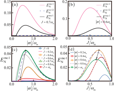
Figure 7: The optimal remote optomechanical entanglement transmission. $\left({\rm{a}}\right)$ The negativity entanglements $E_{\rm{N}}^{{\rm{mc}}\cdot{\rm{1}}}$ (pink dotted line), $E_{\rm{N}}^{{\rm{mc}}\cdot{\rm{2}}}$ (black solid line), and $E_{\rm{N}}^{{\rm{cc}}\cdot{\rm{12}}}$ (blue dashed line) as a function of the normalized detuning $\left|\varpi\right|$ (in units of ${{\omega_{\rm{m}}}}$) with the other parameters set to ${\Delta_{0}}=0$ and $J=0.7{\omega_{\rm{m}}}$. $\left({\rm{b}}\right)$ The negativity entanglements $E_{\rm{N}}^{{\rm{mc}}\cdot{\rm{1}}}$, $E_{\rm{N}}^{{\rm{mc}}\cdot{\rm{2}}}$, and $E_{\rm{N}}^{{\rm{cc}}\cdot{\rm{12}}}$ versus the linear hopping strength $J$ (in units of ${{\omega_{\rm{m}}}}$) with the other parameters set to ${\Delta_{0}}=0$ and $\left|\varpi\right|=0.6{\omega_{\rm{m}}}$. $\left({\rm{c}}\right)$ The negativity entanglements $E_{\rm{N}}^{{\rm{mc}}\cdot{\rm{1}}}$ as a function of $\left|\varpi\right|$ (in units of ${{\omega_{\rm{m}}}}$) for different values of the linear hopping rate: $J=0$ (blue circular line), $J=0.2{\omega_{\rm{m}}}$ (pink solid line), $J=0.4{\omega_{\rm{m}}}$ (orange square line), $J=0.6{\omega_{\rm{m}}}$ (purple dashed line), $J=0.7{\omega_{\rm{m}}}$ (green triangle line), $J=0.8{\omega_{\rm{m}}}$ (brown dotted line), and $J={\omega_{\rm{m}}}$ (red cross line). $\left({\rm{d}}\right)$ The negativity entanglements $E_{\rm{N}}^{{\rm{mc}}\cdot{\rm{1}}}$ as a function of $J$ (in units of ${{\omega_{\rm{m}}}}$) for different values of the normalized detuning: $\left|\varpi\right|=0.2{\omega_{\rm{m}}}$ (blue solid line), $\left|\varpi\right|=0.4{\omega_{\rm{m}}}$ (red square line), $\left|\varpi\right|=0.6{\omega_{\rm{m}}}$ (orange circular line), $\left|\varpi\right|=0.8{\omega_{\rm{m}}}$ (purple dashed line), and $\left|\varpi\right|={\omega_{\rm{m}}}$ (green cross line). The remaining parameter values for $\left({\rm{a}}\right)$-$\left({\rm{d}}\right)$ are set to be the same as in Fig. 4.

In the two-cavity case, we let $E_{\rm{N}}^{{\rm{mc}}\cdot{\rm{1}}}$, $E_{\rm{N}}^{{\rm{mc}}\cdot{\rm{2}}}$, and $E_{\rm{N}}^{{\rm{cc}}\cdot{\rm{12}}}$ denote the logarithmic negativity between the mirror and the cavity 1, the mirror and the cavity 2, and the cavity 1 and the cavity 2, respectively. In Fig. 7$\left({\rm{a}}\right)$, we plot $E_{\rm{N}}^{{\rm{mc}}\cdot{\rm{1}}}$, $E_{\rm{N}}^{{\rm{mc}}\cdot{\rm{2}}}$, and $E_{\rm{N}}^{{\rm{cc}}\cdot{\rm{12}}}$ as functions of the normalized detuning $\left|\varpi\right|$ (in units of ${{\omega_{\rm{m}}}}$) with the other parameters set to ${\Delta_{0}}=0$, $J=0.7{\omega_{\rm{m}}}$, and $T=400{\rm{mK}}$. The normalized detuning $\varpi={\omega_{{{\rm{c}}_{2}}}}-{G_{0}}{Q_{\rm{s}}}$ depends on the steady-state mean values ${Q_{\rm{s}}}={G_{0}}\alpha_{2{\rm{s}}}^{*}{\alpha_{2{\rm{s}}}}/{\omega_{\rm{m}}}$, and ${\alpha_{2{\rm{s}}}}=-iJ{\alpha_{{\rm{1s}}}}/\left({\kappa+i\varpi}\right)$ with ${\alpha_{{\rm{1s}}}}=E/\left[{\kappa+i{\Delta_{0}}+{J^{2}}/\left({\kappa+i\varpi}\right)}\right]$, which can be obtained by setting the time derivation to zero in the nonlinear Langevin equation (42) for ${{N}}=2$. Our numerical findings show that by tuning the magnitude of $\varpi$, we are able to achieve long-distance optomechanical-entanglement transfer. As $\left|\varpi\right|$ increases approximately from $0.50{\omega_{\rm{m}}}$ to $0.65{\omega_{\rm{m}}}$, the distant optomechanical entanglement $E_{\rm{N}}^{{\rm{mc}}\cdot{\rm{1}}}$ correspondingly increases at the expense of the decrease of the neighboring optomechanical entanglement $E_{\rm{N}}^{{\rm{mc}}\cdot{\rm{2}}}$, due to the adjacent cavities acting as entanglement transmitters.

In Fig. 7$\left({\rm{b}}\right)$, we plot $E_{\rm{N}}^{{\rm{mc}}\cdot{\rm{1}}}$, $E_{\rm{N}}^{{\rm{mc}}\cdot{\rm{2}}}$, and $E_{\rm{N}}^{{\rm{cc}}\cdot{\rm{12}}}$ as functions of the linear hopping strength $J$ (in units of ${{\omega_{\rm{m}}}}$) with the other parameters set to ${\Delta_{0}}=0$, $\left|\varpi\right|=0.6{\omega_{\rm{m}}}$, and $T=400{\rm{mK}}$. In a similar analysis, we can also implement distant optomechanical entanglement transfer by adjusting the strength of $J$ approximately from $0.5{\omega_{\rm{m}}}$ to $0.75{\omega_{\rm{m}}}$. In particular, when $T=400{\rm{mK}}$, we find that the optimal remote optomechanical entanglement transfer occurs around $\left|\varpi\right|=0.6$ and $J=0.7$ (in units of ${{\omega_{\rm{m}}}}$), and the maximum value of remote entanglement $E_{\rm{N}}^{{\rm{mc}}\cdot{\rm{1}}}$ is approximately evaluated at $0.045$; see Fig. 7$\left({\rm{c}}\right)$-$\left({\rm{d}}\right)$.

V Summary and Prospect

In summary, we have demonstrated that resonance effects between a mechanical mode and its thermal environment can protect optomechanical entanglement. Specifically, we have shown that resonance effects nearly double the robustness of the optomechanical entanglement against mechanical dissipation and its environmental temperature. The mechanism of optomechanical-entanglement protection involves the elimination of degrees of freedom associated with significant detuning between the mechanical mode and its thermal reservoirs, thereby counteracting the decoherence. We have revealed that this approach is particularly effective when both near-resonant and weak-coupling conditions are simultaneously satisfied between a mechanical mode and its environment. We have also proposed a feasible experimental implementation for the filtering model to observe these phenomena. Furthermore, we extended this theory to an optical cavity array with one oscillating end mirror and investigated optimal optomechanical entanglement transfer. This study represents a significant advancement in the application of resonance effects for protecting quantum systems against decoherence, thereby opening up new possibilities for large-scale quantum information processing and the construction of quantum networks.

In addition, extending the resonance-dominant entanglement theory to non-Markovian and non-Hermitian optomechanical systems is also challenging and expected to be impactful. Specifically, we ensure that studying non-Markovian effects ref-82 ; ref-83 ; ref-84 ; ref-85 , exceptional points ref-86 , parity-time symmetry ref-87 , and anti-parity time symmetry ref-88 on optomechanical entanglement is exciting. In particular, we are interested in future investigations of the optomechanical entanglement properties between resonance states ref-89 ; ref-90 in non-Hermitian systems. This work aims to develop an innovative approach for protecting continuous variable entanglement.

Appendix A Derivation of the Hamiltonian (1)

Here, we show the origin of the total Hamiltonian (1) ref-43 . The total Hamiltonian (1) of this field reservoir consists of two parts, the system (2) and the environment (II.1). Therefore, to obtain Eq. (1), we need to demonstrate the specific origins of Eqs. (2) and (II.1) separately.

To begin with, we show the origin of the system Hamiltonian (2). As usual, for an optomechanical system driven by an optical laser, the Hamiltonian of the composite system can be written as

$$H_{\rm{S}}^{0}=\hbar{\omega_{\rm{c}}}{a^{\dagger}}a+\frac{{{{p^{\prime}}^{2}}}}{{2m}}+\frac{1}{2}m{\left({{\omega_{\rm{m}}}q^{\prime}}\right)^{2}}-\hbar G{a^{\dagger}}aq^{\prime}+i\hbar\left({E{e^{-i{\omega_{0}}t}}{a^{\dagger}}-{E^{*}}{e^{i{\omega_{0}}t}}a}\right),$$ (43)

where a monochromatic field drives the optical mode with the driving frequency ${{\omega_{0}}}$, and the complex amplitude of the driving laser is denoted by $E$. The optical frequency shift per displacement is given by $G=-{{\partial{\omega_{\rm{c}}}\left(x\right)}\mathord{\left/{\vphantom{{\partial{\omega_{\rm{c}}}\left(x\right)}{\partial x}}}\right.\kern-1.2pt}{\partial x}}={{{\omega_{\rm{c}}}}\mathord{\left/{\vphantom{{{\omega_{\rm{c}}}}L}}\right.\kern-1.2pt}L}$. To make the Hamiltonian independent of time, we then move to the rotating frame of the frequency, which makes Eq. (43) as follows:

$${H^{\prime}_{\rm{S}}} = U\left(t\right)H_{\rm{S}}^{0}\left(t\right){U^{\dagger}}\left(t\right)-iU\left(t\right){{\dot{U}}^{\dagger}}\left(t\right)$$ (44)

$$= \hbar{\Delta_{0}}{a^{\dagger}}a+\frac{{{{p^{\prime}}^{2}}}}{{2{{m}}}}+\frac{1}{2}{{m}}{\left({{\omega_{\rm{m}}}q^{\prime}}\right)^{2}}-\hbar{G}{a^{\dagger}}aq^{\prime}+i\hbar\left({E{a^{\dagger}}-{E^{*}}a}\right),$$

where we used the unitary transformation of the form $U\left(t\right)=\exp\left({i{\omega_{0}}{a^{\dagger}}at}\right)$, and ${\Delta_{0}}={\omega_{\rm{c}}}-{\omega_{0}}$ is the detuning of the cavity characteristic frequency ${\omega_{\rm{c}}}$ of the optical cavity from the driving laser frequency ${\omega_{0}}$.

We can make the position and momentum operators dimensionless by defining the zero-point fluctuation amplitude of the mechanical oscillator as ${{{X}}_{{\rm{ZPF}}}}=\sqrt{{\hbar\mathord{\left/{\vphantom{\hbar{2m{\omega_{\rm{m}}}}}}\right.\kern-1.2pt}{2m{\omega_{\rm{m}}}}}}$. Then, we define the dimensionless position operator $q$ and momentum operator $p$ as follows:

$$q=\frac{{q^{\prime}}}{{\sqrt{2}{{X}_{{\rm{ZPF}}}}}}=\frac{1}{{\sqrt{2}}}\left({{b^{\dagger}}+b}\right),\quad p=\frac{{p^{\prime}}}{{\sqrt{2}{{m}}{\omega_{\rm{m}}}{{X}_{{\rm{ZPF}}}}}}=\frac{i}{{\sqrt{2}}}\left({{b^{\dagger}}-b}\right).$$ (45)

Substituting Eq. (45) into Eq. (44), we arrive at

$${H_{\rm{S}}} = \hbar{\Delta_{0}}{a^{\dagger}}a+\frac{\hbar}{2}{\omega_{\rm{m}}}\left({{p^{2}}+{q^{2}}}\right)-\hbar{G_{0}}{a^{\dagger}}aq+i\hbar\left({E{a^{\dagger}}-{E^{*}}a}\right)$$ (46)

$$= \hbar{\Delta_{0}}{a^{\dagger}}a+\hbar{\omega_{\rm{m}}}{b^{\dagger}}b-\hbar{G_{0}}{a^{\dagger}}a\frac{{\left({{b^{\dagger}}+b}\right)}}{{\sqrt{2}}}+i\hbar\left({E{a^{\dagger}}-{E^{*}}a}\right),$$

where ${G_{0}}=\sqrt{2}G{{{X}}_{{\rm{ZPF}}}}={{{\omega_{\rm{c}}}\sqrt{{\hbar\mathord{\left/{\vphantom{\hbar{m{\omega_{\rm{m}}}}}}\right.\kern-1.2pt}{m{\omega_{\rm{m}}}}}}}\mathord{/{\vphantom{{{\omega_{\rm{c}}}\sqrt{{\hbar\mathord{\left/{\vphantom{\hbar{m{\omega_{\rm{m}}}}}}\right.\kern-1.2pt}{m{\omega_{\rm{m}}}}}}}L}}\kern-1.2pt}L}$ is the vacuum optomechanical coupling strength, expressed as a frequency. It quantifies the interaction between a single phonon and a single photon. This produces Eq. (2) in the main text.

Next, we give the origin of the environment Hamiltonian (II.1) for the first time. As is well known from the Bose-Einstein statistics, a heat bath associated with a boson system can be considered as an assembly of harmonic oscillators. This type of heat bath can serve as a model for various physical systems, such as elastic solids (mechanical reservoirs) and electromagnetic fields (optical reservoirs).

Firstly, since in the optomechanical system, both the photons in the optical cavity and the phonons in the mechanical oscillator obey the Bose-Einstein statistics, the free part of the environment can be written in the simple form

$$H_{\rm{E}}^{0}=\frac{1}{2}\sum\limits_{{k}}{\left[{\frac{1}{{m_{{k}}^{\rm{c}}}}{{\left({\tilde{p}_{{k}}^{\rm{c}}}\right)}^{2}}+\Theta_{{k}}^{\rm{c}}{{\left({\tilde{q}_{{k}}^{\rm{c}}}\right)}^{2}}}\right]}+\frac{1}{2}\sum\limits_{{n}}{\left[{\frac{1}{{m_{{n}}^{\rm{m}}}}{{\left({\tilde{p}_{{n}}^{\rm{m}}}\right)}^{2}}+\Theta_{{n}}^{\rm{m}}{{\left({\tilde{q}_{{n}}^{\rm{m}}}\right)}^{2}}}\right]},$$ (47)

where ${m_{{k}}^{\rm{c}}}$ and ${m_{{n}}^{\rm{m}}}$ correspond to the effective mass of the $k$th optical reservoir and $n$th mechanical reservoir, respectively. The momentum and position operators corresponding to the $k$th optical reservoir and the $n$th mechanical reservoir are denoted by ${\tilde{p}_{{k}}^{\rm{c}}}$ ${\tilde{p}_{{n}}^{\rm{m}}}$ and ${\tilde{q}_{{k}}^{\rm{c}}}$ ${\tilde{q}_{{n}}^{\rm{m}}}$, respectively. We set $\Theta_{{k}}^{\rm{c}}=m_{{k}}^{\rm{c}}{\left({{\omega_{{k}}}}\right)^{2}}$ and $\Theta_{{n}}^{\rm{m}}=m_{{n}}^{\rm{m}}{\left({{\omega_{{n}}}}\right)^{2}}$ as the optical and mechanical potential-force constants. The harmonic-oscillator reservoirs have closely spaced frequencies corresponding to photons and phonons, denoted by ${\omega_{k}}$ and ${{\omega_{n}}}$, respectively. Through the process of removing the dimensions from the operators, we can define the dimensionless momentum operators $p_{{k}}^{\rm{c}}$ and ${{p_{{n}}^{\rm{m}}}}$ as well as position operators ${q_{{k}}^{\rm{c}}}$ and ${{q_{{n}}^{\rm{m}}}}$ as follows:

$$p_{{k}}^{\rm{c}} = \sqrt{\frac{{{\omega_{{k}}}}}{{\Theta_{{k}}^{\rm{c}}\hbar}}}\tilde{p}_{{k}}^{\rm{c}}=\sqrt{\frac{1}{{m_{{k}}^{\rm{c}}{\omega_{{k}}}\hbar}}}\tilde{p}_{{k}}^{\rm{c}},\qquad\ q_{{k}}^{\rm{c}}=\sqrt{\frac{{\Theta_{{k}}^{\rm{c}}}}{{{\omega_{{k}}}\hbar}}}\tilde{q}_{{k}}^{\rm{c}}=\sqrt{\frac{{{\omega_{{k}}}}}{\hbar}}\tilde{p}_{{k}}^{\rm{c}},$$ (48)

$$p_{{n}}^{\rm{m}} = \sqrt{\frac{{{\omega_{{n}}}}}{{\Theta_{{n}}^{\rm{m}}\hbar}}}\tilde{p}_{{n}}^{\rm{m}}=\sqrt{\frac{1}{{m_{{n}}^{\rm{m}}{\omega_{{n}}}\hbar}}}\tilde{p}_{{n}}^{\rm{m}},\quad q_{{n}}^{\rm{m}}=\sqrt{\frac{{\Theta_{{n}}^{\rm{m}}}}{{{\omega_{{n}}}\hbar}}}\tilde{q}_{{n}}^{\rm{m}}=\sqrt{\frac{{{\omega_{{n}}}}}{\hbar}}\tilde{p}_{{n}}^{\rm{m}}.$$ (49)

Substituting Eqs. (48) and (49) into Eq. (47), we have

$${H^{\prime}_{\rm{E}}}=\frac{\hbar}{2}\sum\limits_{{k}}{{\omega_{{k}}}\left[{{{\left({p_{{k}}^{\rm{c}}}\right)}^{2}}+{{\left({q_{{k}}^{\rm{c}}}\right)}^{2}}}\right]}+\frac{\hbar}{2}\sum\limits_{{n}}{{\omega_{{n}}}\left[{{{\left({p_{{n}}^{\rm{m}}}\right)}^{2}}+{{\left({q_{{n}}^{\rm{m}}}\right)}^{2}}}\right]},$$ (50)

Secondly, we consider the coupling between the system and the environment. The Hamiltonian of a system can be left arbitrary, such as an atom, as in quantum optics, or a macroscopic LC-circuit. In our case, we treat the optomechanical system as a perturbation to the baths, by writing

$${H^{\prime\prime}_{\rm{E}}} = +\frac{\hbar}{2}\sum\limits_{{k}}{{\omega_{{k}}}\left[{{{\left({p_{{k}}^{\rm{c}}}\right)}^{2}}+{{\left({q_{{k}}^{\rm{c}}+\varepsilon_{{k}}^{\rm{c}}{q_{\rm{c}}}}\right)}^{2}}}\right]}+\frac{\hbar}{2}\sum\limits_{{n}}{{\omega_{{n}}}\left[{{{\left({p_{{n}}^{\rm{m}}-\chi_{{n}}^{\rm{m}}{q_{\rm{m}}}}\right)}^{2}}+{{\left({q_{{n}}^{\rm{m}}}\right)}^{2}}}\right]}$$

$$= +\frac{\hbar}{2}\sum\limits_{{k}}{{\omega_{{k}}}\left[{{{\left({p_{{k}}^{\rm{c}}}\right)}^{2}}+{{\left({q_{{k}}^{\rm{c}}}\right)}^{2}}}\right]}+\frac{\hbar}{2}\sum\limits_{{k}}{{\omega_{{k}}}}{\left({\varepsilon_{{k}}^{\rm{c}}{q_{\rm{c}}}}\right)^{2}}+\hbar\sum\limits_{{k}}{{\omega_{{k}}}}\varepsilon_{{k}}^{\rm{c}}q_{{k}}^{\rm{c}}{q_{\rm{c}}}$$

$$+\frac{\hbar}{2}\sum\limits_{{n}}{{\omega_{{n}}}\left[{{{\left({p_{{n}}^{\rm{m}}}\right)}^{2}}+{{\left({q_{{n}}^{\rm{m}}}\right)}^{2}}}\right]}+\frac{\hbar}{2}\sum\limits_{{n}}{{\omega_{{n}}}{{\left({\chi_{{n}}^{\rm{m}}{q_{\rm{m}}}}\right)}^{2}}-}\hbar\sum\limits_{{n}}{{\omega_{{n}}}}\chi_{{n}}^{\rm{m}}p_{{n}}^{\rm{m}}{q_{\rm{m}}},$$

or

$${{\tilde{H}^{\prime\prime}}_{\rm{E}}} = +\frac{\hbar}{2}\sum\limits_{{k}}{{\omega_{{k}}}\left[{{{\left({p_{{k}}^{\rm{c}}+\varepsilon_{{k}}^{\rm{c}}{p_{\rm{c}}}}\right)}^{2}}+{{\left({q_{{k}}^{\rm{c}}}\right)}^{2}}}\right]}+\frac{\hbar}{2}\sum\limits_{\rm{n}}{{\omega_{{n}}}\left[{{{\left({p_{{n}}^{\rm{m}}-\chi_{{n}}^{\rm{m}}{q_{\rm{m}}}}\right)}^{2}}+{{\left({q_{{n}}^{\rm{m}}}\right)}^{2}}}\right]}$$

$$= +\frac{\hbar}{2}\sum\limits_{\rm{k}}{{\omega_{{k}}}\left[{{{\left({p_{{k}}^{\rm{c}}}\right)}^{2}}+{{\left({q_{{k}}^{\rm{c}}}\right)}^{2}}}\right]}+\frac{\hbar}{2}\sum\limits_{{k}}{{\omega_{{k}}}}{\left({\varepsilon_{{k}}^{\rm{c}}{p_{\rm{c}}}}\right)^{2}}+\hbar\sum\limits_{{k}}{{\omega_{{k}}}}\varepsilon_{{k}}^{\rm{c}}p_{{k}}^{\rm{c}}{p_{\rm{c}}}$$

$$+\frac{\hbar}{2}\sum\limits_{{n}}{{\omega_{{n}}}\left[{{{\left({p_{{n}}^{\rm{m}}}\right)}^{2}}+{{\left({q_{{n}}^{\rm{m}}}\right)}^{2}}}\right]}+\frac{\hbar}{2}\sum\limits_{{n}}{{\omega_{{n}}}{{\left({\chi_{{n}}^{\rm{m}}{q_{\rm{m}}}}\right)}^{2}}-}\hbar\sum\limits_{{n}}{{\omega_{{n}}}}\chi_{{n}}^{\rm{m}}p_{{n}}^{\rm{m}}{q_{\rm{m}}}.$$

The orthogonal relationship for the dimensionless position and momentum operators of the system and the environment read

$${q_{\rm{c}}} = \frac{1}{{\sqrt{2}}}\left({{a^{\dagger}}+a}\right),\ {p_{\rm{c}}}=\frac{i}{{\sqrt{2}}}\left({{a^{\dagger}}-a}\right);\quad\ q_{{k}}^{\rm{c}}=\frac{1}{{\sqrt{2}}}\left({\Gamma_{{k}}^{\dagger}+{\Gamma_{{k}}}}\right),\ p_{{k}}^{\rm{c}}=\frac{i}{{\sqrt{2}}}\left({\Gamma_{{k}}^{\dagger}-{\Gamma_{{k}}}}\right)\!;$$ (53)

$${q_{\rm{m}}} = \frac{1}{{\sqrt{2}}}\left({{b^{\dagger}}+b}\right),\ \ {p_{\rm{c}}}=\frac{i}{{\sqrt{2}}}\left({{b^{\dagger}}-b}\right);\quad q_{{n}}^{\rm{m}}=\frac{1}{{\sqrt{2}}}\left({\Lambda_{{n}}^{\dagger}+{\Lambda_{{n}}}}\right),\ p_{{n}}^{\rm{m}}=\frac{i}{{\sqrt{2}}}\left({\Lambda_{{n}}^{\dagger}-{\Lambda_{{n}}}}\right)\!.$$ (54)

By substituting Eqs. (53)-(54) into the Eqs. (A)-(A) and absorbing terms only of the system operators $0.5\hbar\sum\nolimits_{\rm{k}}{{\omega_{{k}}}{{\left({\varepsilon_{{k}}^{\rm{c}}{p_{\rm{c}}}}\right)}^{2}}}$, $0.5\hbar\sum\nolimits_{{k}}{{\omega_{{k}}}{{\left({\varepsilon_{{k}}^{\rm{c}}{q_{\rm{c}}}}\right)}^{2}}}$, and $0.5\hbar\sum\nolimits_{{n}}{{\omega_{{n}}}{{\left({\chi_{{n}}^{\rm{m}}{q_{\rm{m}}}}\right)}^{2}}}$ into the system Hamiltonian, and further neglecting these higher-order perturbations quantities containing ${\left({\varepsilon_{{k}}^{\rm{c}}}\right)^{2}}$ and ${\left({\chi_{{n}}^{\rm{m}}}\right)^{2}}$, we obtain

$${{\tilde{H}^{\prime\prime}}_{\rm{E}}}\mapsto H_{\rm{E}}^{{q_{\rm{c}}}} = +\hbar\sum\limits_{{k}}{{\omega_{{k}}}}\Gamma_{{k}}^{\dagger}{\Gamma_{{k}}}+\hbar\sum\limits_{{k}}{{g_{{k}}}}\left({\Gamma_{{k}}^{\dagger}{a^{\dagger}}+{\Gamma_{{k}}}a}\right)+\hbar\sum\limits_{{k}}{{g_{{k}}}}\left({\Gamma_{{k}}^{\dagger}a+{\Gamma_{{k}}}{a^{\dagger}}}\right)$$ (55)

$$+\hbar\sum\limits_{{n}}{{\omega_{{n}}}}\Lambda_{{n}}^{\dagger}{\Lambda_{{n}}}-i\hbar\sum\limits_{{n}}{\frac{{{\sigma_{{n}}}}}{2}}\left({\Lambda_{{n}}^{\dagger}-{\Lambda_{{n}}}}\right)\left({{b^{\dagger}}+b}\right),$$

$${{\tilde{H}^{\prime\prime}}_{\rm{E}}}\mapsto H_{\rm{E}}^{{p_{\rm{c}}}} = +\hbar\sum\limits_{{k}}{{\omega_{{k}}}}\Gamma_{{k}}^{\dagger}{\Gamma_{{k}}}-\hbar\sum\limits_{{k}}{{g_{{k}}}}\left({\Gamma_{{k}}^{\dagger}{a^{\dagger}}+{\Gamma_{{k}}}a}\right)+\hbar\sum\limits_{{k}}{{g_{{k}}}}\left({\Gamma_{{k}}^{\dagger}a+{\Gamma_{{k}}}{a^{\dagger}}}\right)$$ (56)

$$+\hbar\sum\limits_{{n}}{{\omega_{{n}}}}\Lambda_{{n}}^{\dagger}{\Lambda_{{n}}}-i\hbar\sum\limits_{{n}}{\frac{{{\sigma_{{n}}}}}{2}}\left({\Lambda_{{n}}^{\dagger}-{\Lambda_{{n}}}}\right)\left({{b^{\dagger}}+b}\right),$$

where we set ${g_{{k}}}=0.5\varepsilon_{{k}}^{\rm{c}}{\omega_{{k}}}$ and ${\sigma_{{n}}}=\chi_{{n}}^{\rm{m}}{\omega_{{n}}}$. The real numbers ${g_{{k}}}$ and ${\sigma_{{n}}}$ represent the coupling strengths between the subsystem and the $n$th reservoir mode, respectively. Finally, we apply the rotating-wave approximation and neglect the counter-rotating terms ${\Gamma_{{k}}^{\dagger}{a^{\dagger}}}$ and ${{\Gamma_{{k}}}a}$ in Eqs. (55) and (56), yielding $H_{\rm{E}}^{{q_{\rm{c}}}}\approx\tilde{H}_{\rm{E}}^{{q_{\rm{c}}}}={H_{\rm{E}}}=\tilde{H}_{\rm{E}}^{{p_{\rm{c}}}}\approx H_{\rm{E}}^{{p_{\rm{c}}}}$, where $\tilde{H}_{\rm{E}}^{{q_{\rm{c}}}}$ and $\tilde{H}_{\rm{E}}^{{q_{\rm{c}}}}$ represent the Hamiltonian after the rotating-wave approximation. This process produces Eq. (II.1) in the main text.

In conclusion, we have physically revealed that photon and phonon perturbations interact with the reservoirs differently. The coupling between photons and the bosonic reservoirs results in the potential energy of the bath depending on the deviation of ${q_{\rm{c}}}$ from all the $q_{{k}}^{\rm{c}}$, while the kinetic energy of the bath depends on the derivation of ${p_{\rm{c}}}$ with respect to all $p_{{k}}^{\rm{c}}$ as well. In other words, it is as if each coordinate $q_{{k}}^{\rm{c}}$ or $p_{{k}}^{\rm{c}}$ is harmonically bound to ${q_{\rm{c}}}$ or ${p_{\rm{c}}}$, respectively. In contrast, the coupling between phonons and the bosonic reservoirs makes the potential energy of the bath depending on the deviation of ${q_{\rm{m}}}$ from all the $p_{{n}}^{\rm{m}}$. The kinetic energy of the bath depends on the derivation of ${p_{\rm{m}}}$ with respect to all $q_{{n}}^{\rm{m}}$ as well. In other words, it is as if each coordinate $q_{{n}}^{\rm{m}}$ or $p_{{n}}^{\rm{m}}$ is harmonically bound to ${p_{\rm{m}}}$ or ${q_{\rm{m}}}$, respectively. In addition, we point out that this difference between perturbations of photons and phonons on the bosonic reservoirs also results in the fact that in the rotating-wave approximation, neglecting the rotating-wave terms ${\Gamma_{{k}}^{\dagger}{a^{\dagger}}}$ and ${{\Gamma_{{k}}}a}$ in the coupling between photons and the electromagnetic field leads to the simplification of $\sum\nolimits_{{k}}{{\omega_{{k}}}[{{{\left({p_{{k}}^{\rm{c}}+\varepsilon_{{k}}^{\rm{c}}{p_{\rm{c}}}}\right)}^{2}}+{{\left({q_{{k}}^{\rm{c}}}\right)}^{2}}}]\approx}\sum\nolimits_{{k}}{{\omega_{{k}}}[{{{\left({p_{{k}}^{\rm{c}}}\right)}^{2}}+{{\left({q_{{k}}^{\rm{c}}+\varepsilon_{{k}}^{\rm{c}}{q_{\rm{c}}}}\right)}^{2}}}]}$, while neglecting the counter-rotating terms $\Lambda_{{n}}^{\dagger}b$ and ${\Lambda_{{n}}}{b^{\dagger}}$ in the coupling between phonons and elastic solid simplifies $\sum\nolimits_{{n}}{{\omega_{{n}}}[{{{\left({p_{{n}}^{\rm{m}}-\chi_{{n}}^{\rm{m}}{q_{\rm{m}}}}\right)}^{2}}+{{\left({q_{{n}}^{\rm{m}}}\right)}^{2}}}]}\approx\sum\nolimits_{{n}}{{\omega_{{n}}}[{{{\left({p_{{n}}^{\rm{m}}}\right)}^{2}}+{{\left({q_{{n}}^{\rm{m}}-\chi_{{n}}^{\rm{m}}{p_{\rm{m}}}}\right)}^{2}}}]}$.

Appendix B Details of the derivation of Eqs. (4)-(6)

In this Appendix, we derive the nonlinear Langevin equations that the total Hamiltonian ${H_{\rm{T}}}$ in Eq. (III.1) satisfies. To begin with, let us derive the nonlinear Langevin equations satisfied by the optical cavity field. The Heisenberg equations of motion for the operator $a$ of the optical cavity field and its corresponding reservoir operators ${\Gamma_{{k}}}$ are given by

$$\dot{a} = \frac{1}{{i\hbar}}\left[{a,{H_{\rm{T}}}}\right]=-i{\Delta_{0}}a+i{G_{0}}a\frac{{\left({{b^{\dagger}}+b}\right)}}{{\sqrt{2}}}+E-i\sum\limits_{{k}}{{g_{{k}}}}{\Gamma_{{k}}},$$ (57)

$${{\dot{\Gamma}}_{{k}}} = \frac{1}{{i\hbar}}\left[{{\Gamma_{{k}}},{H_{\rm{T}}}}\right]=-i{\omega_{{k}}}{\Gamma_{{k}}}-i{g_{{k}}}a.$$ (58)

We are interested in a closed equation for $a$. Equation (58) for ${{\Gamma_{{k}}}}$ can be formally integrated to yield

$${\Gamma_{{k}}}\left(t\right)={\Gamma_{{k}}}\left({{t_{0}}}\right){e^{-i{\omega_{{k}}}\left({t-{t_{0}}}\right)}}-i{g_{{k}}}\int_{{t_{0}}}^{t}{a\left(\tau\right)}{e^{-i{\omega_{{k}}}\left({t-\tau}\right)}}d\tau.$$ (59)

Here the first term describes the free evolution of the reservoir modes, whereas the second term arises from their interaction with the optical cavity field. We eliminate ${\Gamma_{{k}}}$ by substituting Eq. (59) into Eq. (57), finding

$$\dot{a}=-i{\Delta_{0}}a+i{G_{0}}a\frac{{\left({{b^{\dagger}}+b}\right)}}{{\sqrt{2}}}+E-\sum\limits_{{k}}{{{\left({{g_{{k}}}}\right)}^{2}}}\int_{{t_{0}}}^{t}{a\left(\tau\right)}{e^{-i{\omega_{{k}}}\left({t-\tau}\right)}}d\tau+{f_{a}}\left(t\right)$$ (60)

with ${f_{a}}\left(t\right)=-i\sum\nolimits_{{k}}{{g_{{k}}}{\Gamma_{{k}}}\left({{t_{0}}}\right)\exp\left[{-i{\omega_{{k}}}\left({t-{t_{0}}}\right)}\right]}$. In Eq. (60), we can see that the evolution of the system operator depends on the fluctuations in the reservoir.

To proceed, we introduce some approximations. Following the Weisskopf-Wigner approximation ref-46 , we replace the summation over $k$ in Eq. (60) with an integral term, thereby transitioning from a discrete distribution of modes to a continuous one, $\sum\nolimits_{{k}}\mapsto{\left({{L\mathord{\left/{\vphantom{L{2\pi}}}\right.\kern-1.2pt}{2\pi}}}\right)^{3}}\int{{d^{3}}}k$, where $L$ is the length of the sides of the assumed cubic cavity with no specific boundaries, and ${\rm{\mathord{\buildrel\lower 3.0pt\hbox{$\scriptscriptstyle\rightharpoonup$}\over{k}}}}\equiv\left({{k_{x}},{k_{y}},{k_{z}}}\right)$ is the wave vector.

The density of modes between the frequencies $\omega$ and $\omega+d\omega$ can be obtained by transferring from the Cartesian coordinate to the polar coordinate as in ${\rm{\mathord{\buildrel\lower 3.0pt\hbox{$\scriptscriptstyle\rightharpoonup$}\over{k}}}}\equiv\left({{k_{x}},{k_{y}},{k_{z}}}\right)\mapsto\left[{k\sin\left(\theta\right)\cos\left(\phi\right),k\sin\left(\theta\right)\sin\left(\phi\right),k\cos\left(\theta\right)}\right]$. The corresponding volume element in the ${{\rm{\mathord{\buildrel\lower 3.0pt\hbox{$\scriptscriptstyle\rightharpoonup$}\over{k}}}}}$ space is ${d^{3}}k={k^{2}}\sin\left(\theta\right)dkd\theta d\phi=\left({{{{\omega^{2}}}\mathord{\left/{\vphantom{{{\omega^{2}}}{{c^{3}}}}}\right.\kern-1.2pt}{{c^{3}}}}}\right)\sin\left(\theta\right)d\omega d\theta d\phi$. The total number of modes ${N_{a}}$ in the range between $\omega$ and $\omega+d\omega$ is given by $d{N_{a}}={\left({{L\mathord{\left/{\vphantom{L{2\pi c}}}\right.\kern-1.2pt}{2\pi c}}}\right)^{3}}{\omega^{2}}d\omega\int_{0}^{\pi}{\sin\left(\theta\right)}d\theta\int_{0}^{2\pi}{d\phi=\left({{{{L^{3}}{\omega^{2}}}\mathord{\left/{\vphantom{{{L^{3}}{\omega^{2}}}{2{\pi^{2}}{c^{3}}}}}\right.\kern-1.2pt}{2{\pi^{2}}{c^{3}}}}}\right)}d\omega$. A mode density parameter at frequency $\omega$ is therefore given by ${D_{a}}\left(\omega\right)={{d{N_{a}}\left(\omega\right)}\mathord{\left/{\vphantom{{d{N_{a}}\left(\omega\right)}{d\omega=}}}\right.\kern-1.2pt}{d\omega=}}{{{L^{3}}{\omega^{2}}}\mathord{\left/{\vphantom{{{L^{3}}{\omega^{2}}}{2{\pi^{2}}{c^{3}}}}}\right.\kern-1.2pt}{2{\pi^{2}}{c^{3}}}}$, and ${g_{{k}}}=g\left[{{\rm{k}}\left(\omega\right)}\right]=g\left(\omega\right)$ is the coupling constant evaluated at ${\rm{k}}={\omega\mathord{\left/{\vphantom{\omega c}}\right.\kern-1.2pt}c}$. We then approximate this spectrum by a continuous spectrum. Thus, the summation in Eq. (60) can be written as

$$\dot{a}=-i{\Delta_{0}}a+i{G_{0}}a\frac{{\left({{b^{\dagger}}+b}\right)}}{{\sqrt{2}}}+E-\int_{{t_{0}}}^{t}{\int_{0}^{+\infty}{{g^{2}}\left(\omega\right)}{D_{a}}\left(\omega\right){e^{-i\omega\left({t-\tau}\right)}}a\left(\tau\right)d\omega}d\tau+{{f}_{a}}\left(t\right).$$ (61)

Considering an ideal situation, we assume for simplicity that ${\left[{g\left(\omega\right)}\right]^{2}}{D_{a}}\left(\omega\right)={\kappa\mathord{\left/{\vphantom{\kappa\pi}}\right.\kern-1.2pt}\pi}>0$ is constant, so that Eq. (61) is reduced to a simple first-order differential equation ref-47 :

$$\dot{a}=-i{\Delta_{0}}a+i{G_{0}}a\frac{{\left({{b^{\dagger}}+b}\right)}}{{\sqrt{2}}}+E-\frac{{{\kappa}}}{\pi}\int_{{t_{0}}}^{t+{0^{+}}}{\int_{0}^{+\infty}{{e^{-i\omega\left({t-\tau}\right)}}a\left(\tau\right)d\omega}}d\tau+{{f}_{a}}\left(t\right).$$ (62)

Using the relations

$$\int_{0}^{+\infty}{{e^{-i\omega\left({t-\tau}\right)}}d\omega}={\pi}\delta\left({t-\tau}\right),$$ (63)

we arrive at Eq. (6) in the main text:

$$\dot{a}=-\left({{\kappa}+i{\Delta_{0}}}\right)a+i{G_{0}}a\frac{{\left({{b^{\dagger}}+b}\right)}}{{\sqrt{2}}}+E+\sqrt{2{\kappa}}{a_{{\rm{in}}}}$$ (64)

with

$${a_{{\rm{in}}}}\left(t\right)=\frac{{{f_{a}}\left(t\right)}}{{\sqrt{2\kappa}}}=\frac{{-i}}{{\sqrt{2\pi}}}\sum\limits_{{k}}{{g_{{k}}}}\Gamma\left({{t_{0}}}\right){e^{-i{\omega_{{k}}}\left({t-{t_{0}}}\right)}},$$ (65)

where ${a_{{\rm{in}}}}\left(t\right)$ is a noise operator which depends upon the environment operators $\Gamma\left({{t_{0}}}\right)$ at the initial time, and ${{\kappa}}$ is the decay rate of the optical cavity field, which depends on the coupling strength ${{g_{{k}}}}$ of the optical cavity field and its corresponding reservoirs. We have $q={{\left({{b^{\dagger}}+b}\right)}\mathord{/{\vphantom{{\left({{b^{\dagger}}+b}\right)}{\sqrt{2}}}}\kern-1.2pt}{\sqrt{2}}}$ (quadrature definition), and thus we obtain

$$\dot{a}=-\left({{\kappa}+i{\Delta_{0}}}\right)a+i{G_{0}}aq+E+\sqrt{2{\kappa}}{a_{{\rm{in}}}}.$$ (66)

Similarly, the Heisenberg equations of motion for the mechanical operator $b$ and it is corresponding reservoir operators ${\Lambda_{{n}}}$ are given by

$$\dot{b} = \frac{1}{{i\hbar}}\left[{b,{H_{\rm{T}}}}\right]=-i{\omega_{\rm{m}}}b+i\frac{{{G_{0}}}}{{\sqrt{2}}}{a^{\dagger}}a-\frac{1}{{2}}\sum\limits_{{n}}{{\sigma_{{n}}}\left({\Lambda_{{n}}^{\dagger}-{\Lambda_{{n}}}}\right)}$$ (67)

$${{\dot{b}}^{\dagger}} = \frac{1}{{i\hbar}}\left[{{b^{\dagger}},{H_{\rm{T}}}}\right]=i{\omega_{\rm{m}}}{b^{\dagger}}-i\frac{{{G_{0}}}}{{\sqrt{2}}}{a^{\dagger}}a+\frac{1}{{2}}\sum\limits_{{n}}{{\sigma_{{n}}}\left({\Lambda_{{n}}^{\dagger}-{\Lambda_{{n}}}}\right)}$$ (68)

$${{\dot{\Lambda}}_{{n}}} = \frac{1}{{i\hbar}}\left[{{\Lambda_{{n}}},{H_{\rm{T}}}}\right]=-i{\omega_{{n}}}{\Lambda_{{n}}}-{\sigma_{{n}}}\frac{{\left({{b^{\dagger}}+b}\right)}}{{2}}$$ (69)

$$\dot{\Lambda}_{{n}}^{\dagger} = \frac{1}{{i\hbar}}\left[{\Lambda_{{n}}^{\dagger},{H_{\rm{T}}}}\right]=i{\omega_{{n}}}{\Lambda_{{n}}}-{\sigma_{{n}}}\frac{{\left({{b^{\dagger}}+b}\right)}}{{2}}.$$ (70)

Since we have the orthogonal relationship $q={{\left({{b^{\dagger}}+b}\right)}\mathord{\left/{\vphantom{{\left({{b^{\dagger}}+b}\right)}{\sqrt{2}}}}\right.\kern-1.2pt}{\sqrt{2}}}$ and $p={{i\left({{b^{\dagger}}-b}\right)}\mathord{\left/{\vphantom{{i\left({{b^{\dagger}}-b}\right)}{\sqrt{2}}}}\right.\kern-1.2pt}{\sqrt{2}}}$, where $p$ and $q$ are the dimensionless position and momentum operators of the mirror that satisfy the commutation relation $\left[{q,p}\right]=i$. The derivatives of $q$ and $p$ with respect to time read

$$\dot{q} = \frac{1}{{\sqrt{2}}}\left({{{\dot{b}}^{\dagger}}+\dot{b}}\right)={\omega_{\rm{m}}}p,$$ (71)

$$\dot{p} = \frac{i}{{\sqrt{2}}}\left({{{\dot{b}}^{\dagger}}-\dot{b}}\right)=-{\omega_{\rm{m}}}q+{G_{0}}{a^{\dagger}}a+i\sum\limits_{{n}}{{\sigma_{{n}}}\frac{{\left({\Lambda_{{n}}^{\dagger}-{\Lambda_{{n}}}}\right)}}{{\sqrt{2}}}}.$$ (72)

Equation (71) corresponds to Eq. (4) in the main text.

We now focus on a closed equation for $p$. Equations (69)-(70) for ${{\Lambda_{\rm{n}}}}$ and ${\Lambda_{\rm{n}}^{\dagger}}$ can be formally integrated to yield

$${\Lambda_{{n}}}\left(t\right) = {\Lambda_{{n}}}\left({{t_{0}}}\right){e^{-i{\omega_{{n}}}\left({t-{t_{0}}}\right)}}-\frac{1}{{2}}{\sigma_{{n}}}\int_{{t_{0}}}^{t}{\left[{{b^{\dagger}}\left(\tau\right)+b\left(\tau\right)}\right]}{e^{-i{\omega_{\rm{n}}}\left({t-\tau}\right)}}d\tau,$$ (73)

$$\Lambda_{{n}}^{\dagger}\left(t\right) = \Lambda_{{n}}^{\dagger}\left({{t_{0}}}\right){e^{i{\omega_{{n}}}\left({t-{t_{0}}}\right)}}-\frac{1}{{2}}{\sigma_{{n}}}\int_{{t_{0}}}^{t}{\left[{{b^{\dagger}}\left(\tau\right)+b\left(\tau\right)}\right]}{e^{i{\omega_{{n}}}\left({t-\tau}\right)}}d\tau.$$ (74)

We then eliminate the reservoir operators ${\Lambda_{{n}}}$ and $\Lambda_{{n}}^{\dagger}$ by substituting Eqs. (73)-(74) into Eq. (72), and obtain

$$\dot{p}=-{\omega_{\rm{m}}}q+{G_{0}}{a^{\dagger}}a+\Theta+\xi,$$ (75)

where

$$\xi\left(t\right)=\frac{i}{{\sqrt{2}}}\sum\limits_{{n}}{{\sigma_{{n}}}}\left[{\Lambda_{{n}}^{\dagger}\left({{t_{0}}}\right){e^{i{\omega_{{n}}}\left({t-{t_{0}}}\right)}}-{\Lambda_{{n}}}\left({{t_{0}}}\right){e^{-i{\omega_{{n}}}\left({t-{t_{0}}}\right)}}}\right]$$ (76)

and

$$\Theta\left(t\right)={\sum\limits_{{n}}{\left({{\sigma_{{n}}}}\right)}^{2}}\int_{{t_{0}}}^{t}{q\left(\tau\right)}\sin\left[{{\omega_{{n}}}\left({t-\tau}\right)}\right]d\tau.$$ (77)

Equation (76) is the same as Eq. (8) in the main text ref-50 ; ref-91 .

We then integrate Eq. (77) by parts and obtain

$$\Theta\left(t\right)=\sum\limits_{{n}}{\frac{{{{\left({{\sigma_{{n}}}}\right)}^{2}}}}{{{\omega_{{n}}}}}}\left\{{q\left(t\right)\cos\left[{{\omega_{{n}}}\left({t-{t_{0}}}\right)}\right]}\right\}_{{t_{0}}}^{t}-\sum\limits_{{n}}{\frac{{{{\left({{\sigma_{{n}}}}\right)}^{2}}}}{{{\omega_{{n}}}}}}\int_{{t_{0}}}^{t}{\dot{q}\left(\tau\right)}\cos\left[{{\omega_{{n}}}\left({t-\tau}\right)}\right]d\tau.$$ (78)

The integrand function $\varsigma\left(t\right)=\sum\nolimits_{{n}}{{{[{{{\left({{\sigma_{{n}}}}\right)}^{2}}\cos\left({{\omega_{{n}}}t}\right)}]}\mathord{/{\vphantom{{\left[{{{\left({{\sigma_{{n}}}}\right)}^{2}}\cos\left({{\omega_{{n}}}t}\right)}\right]}{{\omega_{{n}}}}}}\kern-1.2pt}{{\omega_{{n}}}}}}$ can be seen to have the form of memory function since it makes the equation of motion at time $t$ depend on the values of $\dot{q}\left(t\right)$ for the previous time. Within the Born-Markov approximation ref-92 , we consider that $\varsigma\left(t\right)$ is a rapidly decaying function and that the equation has a short memory. More precisely, if $\varsigma\left(t\right)$ goes to zero in a time scale that is much less than the time over which $\dot{q}\left(t\right)$ changes, then we can replace $\dot{q}\left(\tau\right)$ by $\dot{q}\left(t\right)$. For $t$ not close to the initial time ${t_{0}}$, we can drop the first term in Eq. (78). Thus, Eq. (78) reads

$$\Theta\left(t\right)\approx-\sum\limits_{{n}}{\frac{{{{\left({{\sigma_{{n}}}}\right)}^{2}}}}{{{\omega_{{n}}}}}}\int_{{t_{0}}}^{t}{\dot{q}\left(t\right)}\cos\left[{{\omega_{{n}}}\left({t-\tau}\right)}\right]d\tau.$$ (79)

Similarly to the optical cavity mode $a$, using the Weisskopf-Winger approximation, we consider the spectrum to be given by the normal modes of a large scale, $L\to+\infty$. A difference between phonons and photons is that ${g_{{k}}}=g\left[{{\rm{k}}\left(\omega\right)}\right]=g\left(\omega\right)$ is the coupling constant evaluated at $\omega\propto{{\rm{k}}^{2}}$. We then approximate this spectrum by a continuous spectrum. Thus, the summation in Eq. (79) can be written as

$$\Theta\left(t\right)\approx-\int_{0}^{+\infty}{\int_{{t_{0}}}^{t}{d\omega d\tau\frac{{{{\left[{\sigma\left(\omega\right)}\right]}^{2}}}}{\omega}\dot{q}\left(t\right)}}\cos\left[{\omega\left({t-\tau}\right)}\right]{D_{b}}\left(\omega\right).$$ (80)

Considering an ideal situation, by setting ${{{{\left[{\sigma\left(\omega\right)}\right]}^{2}}{D_{b}}\left(\omega\right)}\mathord{\left/{\vphantom{{{{\left[{\sigma\left(\omega\right)}\right]}^{2}}{D_{b}}\left(\omega\right)}\omega}}\right.\kern-1.2pt}\omega}={\gamma\mathord{\left/{\vphantom{\gamma\pi}}\right.\kern-1.2pt}\pi}$, we thereby obtain

$$\Theta\left(t\right)\approx-\frac{\gamma}{\pi}\int_{0}^{+\infty}{\int_{{t_{0}}}^{t+{0^{+}}}{d\omega d\tau\dot{q}\left(t\right)}}\cos\left[{\omega\left({t-\tau}\right)}\right].$$ (81)

Using the relations

$$\int_{0}^{+\infty}{\cos\left[{\omega\left({t-\tau}\right)}\right]d\omega}=\pi\delta\left({t-\tau}\right),$$ (82)

and by substituting Eq. (71) into $\Theta\left(t\right)\approx-\gamma\dot{q}\left(t\right)$, we arrive at Eq. (5) in the main text:

$$\dot{p}=-{\omega_{\rm{m}}}q-{\gamma_{\rm{m}}}p+{G_{0}}{a^{\dagger}}a+\xi,$$ (83)

where the mechanical damping rate is ${\gamma_{\rm{m}}}={\omega_{\rm{m}}}\gamma$, which depends on the coupling strength ${{\sigma_{{n}}}}$ and the characteristic frequency of mechanical oscillator ${\omega_{\rm{m}}}$.

Appendix C Details of the derivation of Eqs. (17)-(18)

In this appendix, we focus on deriving the nonlinear Langevin equations satisfied by the filtering model (11) under the dominance of resonance effects. Specifically, we concentrate on the mechanical mode $b$, keeping the optical cavity mode $a$ take the same form as the dynamical Eq. (6). By substituting filtering model (11) into the Heisenberg equation, we obtain

$$\dot{b} = \frac{1}{{i\hbar}}\left[{b,{H_{\rm{T}}}}\right]=-i{\omega_{\rm{m}}}b+i\frac{{{G_{0}}}}{{\sqrt{2}}}{a^{\dagger}}a+\frac{1}{2}\sum\limits_{{n}}{{\sigma_{{n}}}{\Lambda_{{n}}}},$$ (84)

$${{\dot{b}}^{\dagger}} = \frac{1}{{i\hbar}}\left[{{b^{\dagger}},{H_{\rm{T}}}}\right]=i{\omega_{\rm{m}}}{b^{\dagger}}-i\frac{{{G_{0}}}}{{\sqrt{2}}}{a^{\dagger}}a+\frac{1}{{2}}\sum\limits_{{n}}{{\sigma_{{n}}}\Lambda_{{n}}^{\dagger}},$$ (85)

$${{\dot{\Lambda}}_{{n}}} = \frac{1}{{i\hbar}}\left[{{\Lambda_{{n}}},{H_{{\rm{F}}}}}\right]=-i{\omega_{{n}}}{\Lambda_{{n}}}-\frac{{{\sigma_{{n}}}}}{2}b,$$ (86)

$$\dot{\Lambda}_{{n}}^{\dagger} = \frac{1}{{i\hbar}}\left[{\Lambda_{{n}}^{\dagger},{H_{{\rm{F}}}}}\right]=i{\omega_{{n}}}{\Lambda_{{n}}^{\dagger}}-\frac{{{\sigma_{{n}}}}}{2}{b^{\dagger}}.$$ (87)

The derivatives of $p$ and $q$ with respect to time read

$$\dot{q} = \frac{1}{{\sqrt{2}}}\left({{{\dot{b}}^{\dagger}}+\dot{b}}\right)={\omega_{\rm{m}}}p+\frac{1}{2}\sum\limits_{{n}}{{\sigma_{{n}}}{q_{{n}}}},$$ (88)

$$\dot{p} = \frac{i}{{\sqrt{2}}}\left({{{\dot{b}}^{\dagger}}-\dot{b}}\right)=-{\omega_{\rm{m}}}q+{G_{0}}{a^{\dagger}}a+\frac{1}{2}\sum\limits_{{n}}{{\sigma_{{n}}}{p_{{n}}}}.$$ (89)

We are interested in the system operators $p$ and $q$. Equations (86) and (87) for ${\Lambda_{{n}}}$ and ${\Lambda_{{n}}^{\dagger}}$ can be formally integrated to yield

$${\Lambda_{{n}}}\left(t\right) = {\Lambda_{{n}}}\left({{t_{0}}}\right){e^{-i{\omega_{{n}}}\left({t-{t_{0}}}\right)}}-\frac{{{\sigma_{{n}}}}}{2}\int_{{t_{0}}}^{t}{b\left(\tau\right)}{e^{-i{\omega_{{n}}}\left({t-\tau}\right)}}d\tau,$$ (90)

$$\Lambda_{{n}}^{\dagger}\left(t\right) = \Lambda_{{n}}^{\dagger}\left({{t_{0}}}\right){e^{i{\omega_{{n}}}\left({t-{t_{0}}}\right)}}-\frac{{{\sigma_{{n}}}}}{2}\int_{{t_{0}}}^{t}{{b^{\dagger}}\left(\tau\right)}{e^{i{\omega_{{n}}}\left({t-\tau}\right)}}d\tau.$$ (91)

The parts of Eqs. (88) and (89) that contain environmental operators ${q_{{n}}}$ and ${p_{{n}}}$ can be written as

$$\frac{1}{2}\sum\limits_{{n}}{{\sigma_{{n}}}}{q_{{n}}} = \frac{1}{2}\sum\limits_{{n}}{{\sigma_{{n}}}}\frac{{\Lambda_{{n}}^{\dagger}+{\Lambda_{{n}}}}}{{\sqrt{2}}}=\frac{1}{2}\sum\limits_{{n}}{{\sigma_{{n}}}}\frac{1}{{\sqrt{2}}}\left[{\Lambda_{{n}}^{\dagger}\left({{t_{0}}}\right){e^{i{\omega_{{n}}}\left({t-{t_{0}}}\right)}}+{\Lambda_{{n}}}\left({{t_{0}}}\right){e^{-i{\omega_{{n}}}\left({t-{t_{0}}}\right)}}}\right]$$ (92)

$$-{\sum\limits_{{n}}{\left({\frac{{{\sigma_{{n}}}}}{2}}\right)}^{2}}\frac{1}{{\sqrt{2}}}\left[{\int_{{t_{0}}}^{t}{{b^{\dagger}}\left(\tau\right)}{e^{i{\omega_{{n}}}\left({t-\tau}\right)}}d\tau+\int_{{t_{0}}}^{t}{b\left(\tau\right)}{e^{-i{\omega_{{n}}}\left({t-\tau}\right)}}d\tau}\right],$$

$$\frac{1}{2}\sum\limits_{{n}}{{\sigma_{{n}}}{p_{{n}}}} = \frac{1}{2}\sum\limits_{{n}}{{\sigma_{{n}}}}\frac{{i\left({\Lambda_{{n}}^{\dagger}-{\Lambda_{{n}}}}\right)}}{{\sqrt{2}}}=\frac{1}{2}\sum\limits_{{n}}{{\sigma_{{n}}}}\frac{i}{{\sqrt{2}}}\left[{\Lambda_{{n}}^{\dagger}\left({{t_{0}}}\right){e^{i{\omega_{{n}}}\left({t-{t_{0}}}\right)}}-{\Lambda_{{n}}}\left({{t_{0}}}\right){e^{-i{\omega_{{n}}}\left({t-{t_{0}}}\right)}}}\right]$$ (93)

$$-{\sum\limits_{{n}}{\left({\frac{{{\sigma_{{n}}}}}{2}}\right)}^{2}}\frac{i}{{\sqrt{2}}}\left[{\int_{{t_{0}}}^{t}{{b^{\dagger}}\left(\tau\right)}{e^{i{\omega_{{n}}}\left({t-\tau}\right)}}d\tau-\int_{{t_{0}}}^{t}{b\left(\tau\right)}{e^{-i{\omega_{{n}}}\left({t-\tau}\right)}}d\tau}\right].$$

For convenience, we concisely express Eqs. (92) and (93) as

$$\frac{1}{2}\sum\limits_{{n}}{{\sigma_{{n}}}}{q_{{n}}} = \frac{1}{2}\xi^{\prime}\left(t\right)-\chi^{\prime}\left(t\right),$$ (94)

$$\frac{1}{2}\sum\limits_{{n}}{{\sigma_{{n}}}{p_{{n}}}} = \frac{1}{2}\xi\left(t\right)-\chi\left(t\right),$$ (95)

where

$$\xi^{\prime}\left(t\right) = \sum\limits_{{n}}{{\sigma_{{n}}}}\frac{1}{{\sqrt{2}}}\left[{\Lambda_{{n}}^{\dagger}\left({{t_{0}}}\right){e^{i{\omega_{{n}}}\left({t-{t_{0}}}\right)}}+{\Lambda_{{n}}}\left({{t_{0}}}\right){e^{-i{\omega_{{n}}}\left({t-{t_{0}}}\right)}}}\right],$$ (96)

$$\xi\left(t\right) = \sum\limits_{{n}}{{\sigma_{{n}}}}\frac{i}{{\sqrt{2}}}\left[{\Lambda_{{n}}^{\dagger}\left({{t_{0}}}\right){e^{i{\omega_{{n}}}\left({t-{t_{0}}}\right)}}-{\Lambda_{{n}}}\left({{t_{0}}}\right){e^{-i{\omega_{{n}}}\left({t-{t_{0}}}\right)}}}\right],$$ (97)

$$\chi^{\prime}\left(t\right) = \sum\limits_{{n}}{{{\left({\frac{{{\sigma_{{n}}}}}{2}}\right)}^{2}}\int_{{t_{0}}}^{t}{\left\{{{q}\left(\tau\right)\cos\left[{{\omega_{{n}}}\left({t-\tau}\right)}\right]+{p}\left(\tau\right)\sin\left[{{\omega_{{n}}}\left({t-\tau}\right)}\right]}\right\}}d\tau},$$ (98)

$$\chi\left(t\right) = \sum\limits_{{n}}{{{\left({\frac{{{\sigma_{{n}}}}}{2}}\right)}^{2}}\int_{{t_{0}}}^{t}{\left\{{{p}\left(\tau\right)\cos\left[{{\omega_{{n}}}\left({t-\tau}\right)}\right]-{q}\left(\tau\right)\sin\left[{{\omega_{{n}}}\left({t-\tau}\right)}\right]}\right\}}d\tau}.$$ (99)

Next, we make some approximations. In a similar way to Appendix B, under the Born-Markov and Weisskopf-Wigner approximations, Eqs. (98) and (99) become

$$\chi^{\prime}\left(t\right)\!\! = \!\!\frac{1}{4}\int_{0}^{+\infty}\!\!{\int_{{t_{0}}}^{t+{0^{+}}}{\!\!\!\!d\tau d\omega\left\{{\dot{q}\left(t\right)\sin\left[{\omega\left({t-\tau}\right)}\right]-\dot{p}\left(t\right)\cos\left[{\omega\left({t-\tau}\right)}\right]}\right\}\frac{{{{\left[{\sigma\left(\omega\right)}\right]}^{2}}{D_{b}}\left(\omega\right)}}{\omega}}}\!,$$ (100)

$$\chi\left(t\right)\!\! = \!\!\frac{1}{4}\int_{0}^{+\infty}\!\!{\int_{{t_{0}}}^{t+{0^{+}}}{\!\!\!\!d\tau d\omega\left\{{\dot{p}\left(t\right)\sin\left[{\omega\left({t-\tau}\right)}\right]+\dot{q}\left(t\right)\cos\left[{\omega\left({t-\tau}\right)}\right]}\right\}\frac{{{{\left[{\sigma\left(\omega\right)}\right]}^{2}}{D_{b}}\left(\omega\right)}}{\omega}}}\!.$$ (101)

Furthermore, we set ${{{{\left[{\sigma\left(\omega\right)}\right]}^{2}}{D_{b}}(\omega)}\mathord{/{\vphantom{{{{\left[{\sigma\left(\omega\right)}\right]}^{2}}{D_{b}}\left(\omega\right)}\omega}}\kern-1.2pt}\omega}={\gamma\mathord{\left/{\vphantom{\gamma\pi}}\right.\kern-1.2pt}\pi}$. Then, by using the relation $\int_{0}^{+\infty}{\cos\left[{\omega\left({t-\tau}\right)}\right]d\omega}=\pi\delta\left({t-\tau}\right)$ and $\int_{0}^{+\infty}{\sin\left[{\omega\left({t-\tau}\right)}\right]d\omega=}0$, we find $\chi^{\prime}\left(t\right)={{-\gamma\dot{p}\left(t\right)}\mathord{\left/{\vphantom{{-\gamma\dot{p}\left(t\right)}4}}\right.\kern-1.2pt}4}$ and $\chi\left(t\right)={{\gamma\dot{q}\left(t\right)}\mathord{\left/{\vphantom{{\gamma\dot{q}\left(t\right)}4}}\right.\kern-1.2pt}4}$.

Finally, Eqs. (88) and (89) can be rewritten as

$$\dot{q} = {\omega_{\rm{m}}}p+\frac{\gamma}{4}\dot{p}+\frac{1}{2}\xi^{\prime},$$ (102)

$$\dot{p} = -{\omega_{\rm{m}}}q-\frac{\gamma}{4}\dot{q}+{G_{0}}{a^{\dagger}}a+\frac{1}{2}\xi\left(t\right).$$ (103)

Substituting ${\dot{p}}$ and ${\dot{q}}$ into Eqs. (102) and (103), respectively, we obtain after decoupling

$$\left({1+\frac{{{\gamma^{2}}}}{{16}}}\right)\dot{q} = {\omega_{\rm{m}}}p-\frac{{{\gamma_{\rm{m}}}}}{4}q+\frac{\gamma}{4}{G_{0}}{a^{\dagger}}a+\frac{\gamma}{8}\xi+\frac{1}{2}\xi^{\prime},$$ (104)

$$\left({1+\frac{{{\gamma^{2}}}}{{16}}}\right)\dot{p} = -{\omega_{\rm{m}}}q-\frac{{{\gamma_{\rm{m}}}}}{4}p+{G_{0}}{a^{\dagger}}a-\frac{\gamma}{8}\xi^{\prime}+\frac{1}{2}\xi,$$ (105)

where we set the mechanical damping rate as ${\gamma_{\rm{m}}}={\omega_{\rm{m}}}\gamma$. Under the weak coupling limit $\gamma\ll 1$, we neglect the small terms in Eqs. (104) and (105) that contain quantities of ${\gamma^{2}}$ and $\gamma$. We ultimately reproduce the same Eqs. (17) and (18) as those presented in the main text.

Appendix D Details of the derivation of the Lyapunov equation (35)

This Appendix derives the Lyapunov equation (35). We begin with the definition of the covariance matrix. According to the definition ref-93 , any matrix element of the covariance matrix can be expressed as

$${{{V}}_{{{ij}}}}\left(t\right)=\frac{1}{2}\left\langle{{\mu_{{i}}}\left(t\right){\mu_{{j}}}\left(t\right)+{\mu_{{j}}}\left(t\right){\mu_{{i}}}\left(t\right)}\right\rangle,$$ (106)

which satisfies the differential equation

$$\frac{{d{{{V}}_{{{ij}}}}\left(t\right)}}{{dt}}=\frac{1}{2}\left\langle{\frac{{d{\mu_{{i}}}\left(t\right)}}{{dt}}{\mu_{{j}}}\left(t\right)+{\mu_{{i}}}\left(t\right)\frac{{d{\mu_{{j}}}\left(t\right)}}{{dt}}+\frac{{d{\mu_{{j}}}\left(t\right)}}{{dt}}{\mu_{{i}}}\left(t\right)+{\mu_{{j}}}\left(t\right)\frac{{d{\mu_{{i}}}\left(t\right)}}{{dt}}}\right\rangle.$$ (107)

The matrix elements of the differential Eq. (107) read

$${{\dot{\mu}}_{{i}}}\left(t\right)=\sum\limits_{{o}}{{{{A}}_{{{io}}}}{\mu_{{i}}}\left(t\right)+{n_{{i}}}\left(t\right)}.$$ (108)

Substituting Eq. (108) into Eq. (107), we obtain

$$\frac{{d{{{V}}_{{{ij}}}}\left(t\right)}}{{dt}} = +\frac{1}{2}\left\langle{\left[{\sum\limits_{{o}}{{{{A}}_{{{io}}}}{\mu_{{o}}}\left(t\right)+{n_{{i}}}\left(t\right)}}\right]{\mu_{{j}}}\left(t\right)+{\mu_{{i}}}\left(t\right)\left[{\sum\limits_{{o}}{{{{A}}_{{{jo}}}}{\mu_{{o}}}\left(t\right)+{n_{{j}}}\left(t\right)}}\right]}\right\rangle$$ (109)

$$+\frac{1}{2}\left\langle{\left[{\sum\limits_{{o}}{{{{A}}_{{{jo}}}}{\mu_{{o}}}\left(t\right)+{n_{{j}}}\left(t\right)}}\right]{\mu_{{i}}}\left(t\right)+{\mu_{{j}}}\left(t\right)\left[{\sum\limits_{{o}}{{{{A}}_{{{io}}}}{\mu_{{o}}}\left(t\right)+{n_{{i}}}\left(t\right)}}\right]}\right\rangle$$

$$= \sum\limits_{{o}}{{{{A}}_{{{io}}}}\left(t\right)}{{{V}}_{{{oj}}}}\left(t\right)+\sum\limits_{{o}}{{{{A}}_{{{jo}}}}\left(t\right)}{{{V}}_{{{io}}}}\left(t\right)+{D_{{{ij}}}\left(t\right)},$$

where

$${D_{{{ij}}}}\left(t\right)=\frac{{\left\langle{{n_{{i}}}\left(t\right){\mu_{{j}}}\left(t\right)}\right\rangle+\left\langle{{\mu_{{i}}}\left(t\right){n_{{j}}}\left(t\right)}\right\rangle+\left\langle{{n_{{j}}}\left(t\right){\mu_{{i}}}\left(t\right)}\right\rangle+\left\langle{{\mu_{{j}}}\left(t\right){n_{{i}}}\left(t\right)}\right\rangle}}{2}.$$ (110)

We then calculate each term in ${D_{{\rm{ij}}}}$. For example, we have

$$\left\langle{{n_{{i}}}\left(t\right){\mu_{{j}}}\left(t\right)}\right\rangle = \left\langle{{n_{{i}}}\left(t\right)\sum\limits_{{o}}{\left[{{{M}_{{{jo}}}}\left({t,{t_{0}}}\right){\mu_{{o}}}\left({{t_{0}}}\right)+\int_{{t_{0}}}^{t}{{{M}_{{{jo}}}}\left({t,\tau}\right){n_{{o}}}\left(\tau\right)d\tau}}\right]}}\right\rangle$$ (111)

$$= \sum\limits_{{o}}{{{M}_{{{jo}}}}\left({t,{t_{0}}}\right)\left\langle{{n_{{i}}}\left(t\right){\mu_{{o}}}\left({{t_{0}}}\right)}\right\rangle}+\sum\limits_{{o}}{\int_{{t_{0}}}^{t}{{{M}_{{{jo}}}}\left({t,\tau}\right)\left\langle{{n_{{i}}}\left(t\right){n_{{j}}}\left(\tau\right)}\right\rangle d\tau}}$$

$$= \sum\limits_{{o}}{\int_{{t_{0}}}^{t}{{{M}_{{{jo}}}}\left({t,\tau}\right)\left\langle{{n_{{i}}}\left(t\right){n_{{j}}}\left(\tau\right)}\right\rangle d\tau}},$$

where ${M}\left(t\right)=\exp\left({{A}t}\right)$. Similarly, we obtain the other terms in ${D_{{{ij}}}}$, which are

$$\left\langle{{\mu_{\rm{i}}}\left(t\right){n_{\rm{j}}}\left(t\right)}\right\rangle = \sum\limits_{\rm{o}}{\int_{{t_{0}}}^{t}{{{\rm{M}}_{{\rm{io}}}}\left({t,\tau}\right)\left\langle{{n_{\rm{o}}}\left(\tau\right){n_{\rm{j}}}\left(t\right)}\right\rangle d\tau}},$$ (112)

$$\left\langle{{n_{\rm{j}}}\left(t\right){\mu_{\rm{i}}}\left(t\right)}\right\rangle = \sum\limits_{\rm{o}}{\int_{{t_{0}}}^{t}{{{\rm{M}}_{{\rm{io}}}}\left({t,\tau}\right)\left\langle{{n_{\rm{j}}}\left(t\right){n_{\rm{o}}}\left(\tau\right)}\right\rangle d\tau}},$$ (113)

$$\left\langle{{\mu_{\rm{j}}}\left(t\right){n_{\rm{i}}}\left(t\right)}\right\rangle = \sum\limits_{\rm{o}}{\int_{{t_{0}}}^{t}{{{\rm{M}}_{{\rm{jo}}}}\left({t,\tau}\right)\left\langle{{n_{\rm{o}}}\left(\tau\right){n_{\rm{i}}}\left(t\right)}\right\rangle d\tau}}.$$ (114)

Hence, ${D_{{{ij}}}}$ can be written as

$${D_{{{ij}}}}=\sum\limits_{{o}}{\int_{{t_{0}}}^{t}{{{M}_{{{jo}}}}\left({t,\tau}\right)\Phi_{{{io}}}^{\left(1\right)}\left({t,\tau}\right)d\tau}}+\sum\limits_{{o}}{\int_{{t_{0}}}^{t}{{M_{{{io}}}}\left({t,\tau}\right)\Phi_{{{oj}}}^{\left(2\right)}\left({t,\tau}\right)d\tau}},$$ (115)

where

$$\Phi_{{{io}}}^{\left(1\right)}\left({t,\tau}\right) = \frac{1}{2}\left\langle{{n_{{i}}}\left(t\right){n_{{o}}}\left(\tau\right)+{n_{{o}}}\left(\tau\right){n_{{i}}}\left(t\right)}\right\rangle,$$ (116)

$$\Phi_{{{oj}}}^{\left(2\right)}\left({t,\tau}\right) = \frac{1}{2}\left\langle{{n_{{o}}}\left(\tau\right){n_{{j}}}\left(t\right)+{n_{{j}}}\left(t\right){n_{{o}}}\left(\tau\right)}\right\rangle.$$ (117)

The transposes of the column vector of noise operators are given by ${n^{T}}\left(t\right)=\left[{0.5\xi^{\prime}\left(t\right),0.5\xi\left(t\right),\sqrt{2\kappa}{X_{{\rm{in}}}}\left(t\right),\sqrt{2\kappa}{Y_{{\rm{in}}}}\left(t\right)}\right]$, we note that the non-zero correlation functions satisfy the following relations:

$$2\left\langle{{X_{{\rm{in}}}}\left(t\right){Y_{{\rm{in}}}}\left(\tau\right)}\right\rangle = -2\left\langle{{Y_{{\rm{in}}}}\left(t\right){X_{{\rm{in}}}}\left(\tau\right)}\right\rangle=-i\delta\left({t-\tau}\right),$$ (118)

$$2\left\langle{{X_{{\rm{in}}}}\left(t\right){X_{{\rm{in}}}}\left(\tau\right)}\right\rangle = 2\left\langle{{Y_{{\rm{in}}}}\left(t\right){Y_{{\rm{in}}}}\left(\tau\right)}\right\rangle=\left({2{{{{\bar{n}}}}_{a}}+1}\right)\delta\left({t-\tau}\right),$$ (119)

$$\left\langle{\xi\left(t\right)\xi\left(\tau\right)+\xi\left(\tau\right)\xi\left(t\right)}\right\rangle = \left\langle{\xi^{\prime}\left(t\right)\xi^{\prime}\left(\tau\right)+\xi^{\prime}\left(\tau\right)\xi^{\prime}\left(t\right)}\right\rangle=2{\gamma_{\rm{m}}}\left({2{{\bar{n}}}+1}\right)\delta\left({t-\tau}\right).$$ (120)

To be concise, we set ${{{{\rm{\bar{n}}}}_{a}}}$ equal to zero. Using the relation (118)-(120), we calculate each term of $\Phi_{{{io}}}^{\left(1\right)}\left({t,\tau}\right)$ and $\Phi_{{{oj}}}^{\left(2\right)}\left({t,\tau}\right)$. The result is given by

$$\Phi_{{{io}}}^{\left(1\right)}=\left({\begin{array}[]{*{20}{c}}{\Phi_{11}^{\left(1\right)}}&{\Phi_{12}^{\left(1\right)}}&{\Phi_{13}^{\left(1\right)}}&{\Phi_{14}^{\left(1\right)}}\\ {\Phi_{21}^{\left(1\right)}}&{\Phi_{22}^{\left(1\right)}}&{\Phi_{23}^{\left(1\right)}}&{\Phi_{24}^{\left(1\right)}}\\ {\Phi_{31}^{\left(1\right)}}&{\Phi_{32}^{\left(1\right)}}&{\Phi_{33}^{\left(1\right)}}&{\Phi_{34}^{\left(1\right)}}\\ {\Phi_{41}^{\left(1\right)}}&{\Phi_{42}^{\left(1\right)}}&{\Phi_{43}^{\left(1\right)}}&{\Phi_{44}^{\left(1\right)}}\end{array}}\right)={{{D}}_{{{io}}}}\delta\left({t-\tau}\right),$$ (125)

where ${{{D}}_{{{io}}}}{\rm{=Diag}}\left[{{{{\gamma_{\rm{m}}}\left({2{{\bar{n}}}+1}\right)}\mathord{\left/{\vphantom{{{\gamma_{\rm{m}}}\left({2{{\bar{n}}}+1}\right)}4}}\right.\kern-1.2pt}4},{{{\gamma_{\rm{m}}}\left({2{{\bar{n}}}+1}\right)}\mathord{\left/{\vphantom{{{\gamma_{\rm{m}}}\left({2{{\bar{n}}}+1}\right)}4}}\right.\kern-1.2pt}4},\kappa,\kappa}\right]$.

Similarly, we obtain $\Phi_{{{oj}}}^{\left(2\right)}={{{D}}_{{{oj}}}}\delta\left({t-\tau}\right)={\rm{Diag}}\left[{{{{\gamma_{\rm{m}}}\left({2{{\bar{n}}}+1}\right)}\mathord{\left/{\vphantom{{{\gamma_{\rm{m}}}\left({2{{\bar{n}}}+1}\right)}4}}\right.\kern-1.2pt}4},{{{\gamma_{\rm{m}}}\left({2{{\bar{n}}}+1}\right)}\mathord{\left/{\vphantom{{{\gamma_{\rm{m}}}\left({2{{\bar{n}}}+1}\right)}4}}\right.\kern-1.2pt}4},\kappa,\kappa}\right]\delta\left({t-\tau}\right)$. Therefore, Eq. (115) can be rewritten as

$${{{D}}_{{{ij}}}} = \sum\limits_{{o}}{\int_{{t_{0}}}^{t}{{{M}_{{{jo}}}}\left({t,\tau}\right)\Phi_{{{io}}}^{\left(1\right)}\left({t,\tau}\right)d\tau}}+\sum\limits_{{o}}{\int_{0}^{t}{{{M}_{{{io}}}}\left({t,\tau}\right)\Phi_{{{oj}}}^{\left(2\right)}\left({t,\tau}\right)d\tau}}$$ (126)

$$= \sum\limits_{{o}}{\int_{{t_{0}}}^{t}{{{M}_{{{jo}}}}\left({t,\tau}\right){{{D}}_{{{io}}}}\delta\left({t-\tau}\right)d\tau}}+\sum\limits_{{o}}{\int_{{t_{0}}}^{t}{{{M}_{{{io}}}}\left({t,\tau}\right){{{D}}_{{{oj}}}}\delta\left({t-\tau}\right)d\tau}}$$

$$= \frac{1}{2}\sum\limits_{{o}}{{{\rm I}_{{{jo}}}}{{{D}}_{{{io}}}}+}\frac{1}{2}\sum\limits_{{o}}{{{\rm I}_{{{io}}}}{{{D}}_{{{oj}}}}}=\frac{1}{2}\sum\limits_{{o}}{{{{D}}_{{{io}}}}{\rm{I}}_{{{oj}}}^{T}+}\frac{1}{2}\sum\limits_{{o}}{{{\rm{I}}_{{{io}}}}{{{D}}_{{{oj}}}}}\equiv{{D}},$$

where ${{D={\rm{Diag}}}}\left[{{{{\gamma_{\rm{m}}}\left({2{{\bar{n}}}+1}\right)}\mathord{\left/{\vphantom{{{\gamma_{\rm{m}}}\left({2{{\bar{n}}}+1}\right)}4}}\right.\kern-1.2pt}4},{{{\gamma_{\rm{m}}}\left({2{{\bar{n}}}+1}\right)}\mathord{\left/{\vphantom{{{\gamma_{\rm{m}}}\left({2{{\bar{n}}}+1}\right)}4}}\right.\kern-1.2pt}4},\kappa,\kappa}\right]$.

Thus, Eq. (109) reads ${{\dot{V}=}}{A}{{V+V}}{{A}^{T}}+D$. When the stability conditions are satisfied, in the long-time limit, the derivative of the covariance matrix with respect to time approaches zero, ${{\dot{V}}}=0$. This produces the Lyapunov equation (35) in the main text, ${{AV}}+{{V}}{{{A}}^{T}}=-{{D}}$.

References

• (1) E. Schrödinger, Die gegenwärtige situation in der quantenmechanik, Sci. Nat., 23(48): 807-812 (1935).
• (2) J. S. Bell, On the Einstein Podolsky Rosen paradox, Physics Physique Fizika 1, 195 (1964).
• (3) D. Bouwmeester, A. Ekert, and A. Zeilinger, The Physics of Quantum Information (Springer, Berlin, 2000).
• (4) F. J. Duarte and T. Taylor, Quantum Entanglement Engineering and Applications (IOP Press, London, 2021).
• (5) A. Streltsov, G. Adesso, and M. B. Plenio, Colloquium: Quantum coherence as a resource, Rev. Mod. Phys. 89, 041003 (2017).
• (6) S. Takeda, M. Fuwa, P. van Loock, and A. Furusawa, Entanglement Swapping between Discrete and Continuous Variables, Phys. Rev. Lett. 114, 100501 (2015).
• (7) G. Masada, K. Miyata, A. Politi, T. Hashimoto, J. L. O’Brien, and A. Furusawa, Continuous-variable entanglement on a chip, Nature Photonics 9, 316-319 (2015).
• (8) D. Estève, J.-M. Raimond, and J. Dalibard, Quantum Entanglement and Information Processing (Elsevier, Amsterdam, 2003).
• (9) W. K. Wootters, Entanglement of Formation of an Arbitrary State of Two Qubits, Phys. Rev. Lett. 80, 2245 (1998).
• (10) A. Miranowicz and A. Grudka, Ordering two-qubit states with concurrence and negativity, Phys. Rev. A 70, 032326 (2004).
• (11) I. Bengtsson and K. Życzkowski, Geometry of Quantum States: An Introduction to Quantum Entanglement (Cambridge University Press, UK, 2006).
• (12) V. Vedral, Quantifying entanglement in macroscopic systems, Nature 453(7198): 1004-1007 (2008).
• (13) L.-M. Duan, G. Giedke, J. I. Cirac, and P. Zoller, Entanglement purification of Gaussian Continuous Variable Quantum States, Phys. Rev. Lett. 84, 4002 (2000).
• (14) W. P. Bowen, R. Schnabel, P. K. Lam, and T. C. Ralph, Experimental Investigation of Criteria for Continuous Variable Entanglement, Phys. Rev. Lett. 90, 043601 (2003).
• (15) S. P. Walborn, B. G. Taketani, A. Salles, F. Toscano, and R. L. de Matos Filho, Entropic Entanglement Criteria for Continuous Variables, Phys. Rev. Lett. 103, 160505 (2009).
• (16) R. Horodecki, P. Horodecki, M. Horodecki, and K. Horodecki, Quantum entanglement, Rev. Mod. Phys. 81, 865 (2009).
• (17) C. M. Caves, Quantum-Mechanical Radiation-Pressure Fluctuations in an Interferometer, Phys. Rev. Lett. 45, 75 (1980).
• (18) M. Aspelmeyer, T. J. Kippenberg, and F. Marquardt, Cavity optomechanics, Rev. Mod. Phys. 86, 1391 (2014).
• (19) A. Bachtold, J. Moser, and M. I. Dykman, Mesoscopic physics of nanomechanical systems, Rev. Mod. Phys. 94, 045005 (2022).
• (20) M. Aspelmeyer, P. Meystre, and K. Schwab, Quantum optomechanics, Phys. Today 65(7), 29 (2012).
• (21) M. Aspelmeyer, T. J. Kippenberg, and F. Marquardt, Cavity Optomechanics: Nano- and Micromechanical Resonators Interacting with Light (Springer, Germany, 2014).
• (22) S. L. Braunstein and P. van Loock, Quantum information with continuous variables, Rev. Mod. Phys. 77, 513 (2005).
• (23) M. A. Macovei and A. Pálffy, Multiphonon quantum dynamics in cavity optomechanical systems, Phys. Rev. A 105, 033503 (2022).
• (24) D. Vitali, S. Gigan, A. Ferreira, H. R. Böhm, P. Tombesi, A. Guerreiro, V. Vedral, A. Zeilinger, and M. Aspelmeyer, Optomechanical Entanglement between a Movable Mirror and a Cavity Field, Phys. Rev. Lett. 98, 030405 (2007).
• (25) K. Y. Dixon, L. Cohen, N. Bhusal, C. Wipf, J. P. Dowling, and T. Corbitt, Optomechanical entanglement at room temperature: A simulation study with realistic conditions, Phys. Rev. A 102, 063518 (2020).
• (26) M. B. Plenio, Logarithmic Negativity: A Full Entanglement Monotone That is not Convex, Phys. Rev. Lett. 95, 090503 (2005).
• (27) D.-G. Lai, J.-Q. Liao, A. Miranowicz, and F. Nori, Noise-Tolerant Optomechanical Entanglement via Synthetic Magnetism, Phys. Rev. Lett. 129, 063602 (2022).
• (28) J.-X. Liu, Y.-F. Jiao, Y. Li, X.-W. Xu, Q.-Y. He, H. Jing, Phased-controlled asymmetric optomechanical entanglement against optical backscattering, Sci. China Phys. Mech. Astron. 66, 230312 (2023).
• (29) Y.-F. Jiao, S.-D. Zhang, Y.-L. Zhang, A. Miranowicz, L.-M. Kuang, and H. Jing, Nonreciprocal Optomechanical Entanglement against Backscattering Losses, Phys. Rev. Lett. 125, 143605 (2020).
• (30) Cheng Shang, H. Z. Shen, and X. X. Yi, Nonreciprocity in a strong coupled three-mode optomechanical circulatory system, Optics Express 27, 18 (2019).
• (31) J. Huang, D.-G. Lai, and J.-Q. Liao, Thermal-noise-resistant optomechanical entanglement via general dark-mode control, Phys. Rev. A 106, 063506 (2022).
• (32) G. D. Chiara, M. Paternostro, and G. M. Palma, Entanglement detection in hybrid optomechanical systems, Phys. Rev. A 83, 052324 (2011).
• (33) L. Zhou, Y. Han, J. T. Jing, and W. P. Zhang, Entanglement of nanomechanical oscillators and two-mode fields induced by atomic coherence, Phys. Rev. A 83, 052117 (2011).
• (34) Cheng Shang, Coupling enhancement and symmetrization of single-photon optomechanics in open quantum systems, arXiv: 2302. 04897 (2023).
• (35) M. Bekele, T. Yirgashewa, and S. Tesfa, Entanglement of mechanical modes in a doubly resonant optomechanical cavity of a correlated emission laser, Phys. Rev. A 107, 012417 (2003).
• (36) M. Bekele, T. Yirgashewa, and S. Tesfa, Effects of a three-level laser on mechanical squeezing in a doubly resonant optomechanical cavity coupled to biased noise fluctuations, Phys. Rev. A 105, 053502 (2022).
• (37) Y.-Q Shi, L. Cong, and H.-P. Eckle, Entanglement resonance in the asymmetric quantum Rabi model, Phys. Rev. A 105, 062450 (2022).
• (38) R. Ghobadi, S. Kumar, B. Pepper, D. Bouwmeester, A. I. Lvovsky, and C. Simon, Optomechanical Micro-Macro Entanglement, Phys. Rev. Lett. 112, 080503 (2014).
• (39) C. Gut, K. Winkler, J. H.-Obermaier, S. G. Hofer, R. M. Nia, N. Walk, A. Steffens, J. Eisert, W. Wieczorek, J. A. Slater, M. Aspelmeyer, and K. Hammerer, Stationary optomechanical entanglement between a mechanical oscillator and its measurement apparatus, Phys. Rev. Research 2, 033244 (2020).
• (40) J. Kohler, N. Spethmann, S. Schreppler, and D. M. S.-Kurn, Cavity-Assisted Measurement and Coherent Control of Collective Atomic Spin Oscillators, Phys. Rev. Lett. 118, 063604 (2017).
• (41) H. Y. Sun, Cheng Shang, X. X. Luo, Y. H. Zhou, and H. Z. Shen, Optical-assisted Photon Blockade in a Cavity System via Parametric Interactions, Int. J. Theor. Phys 58, 3640 (2019).
• (42) C. K. Law, Interaction between a moving mirror and radiation pressure: A Hamiltonian formulation, Phys. Rev. A 51, 2537 (1995).
• (43) T. A. Palomaki, J. D. Teufel, R. W. Simmonds, and K. W. Lehnert, Entangling Mechanical Motion with Microwave Fields, Science 342, 710 (2013).
• (44) J. Chan, T. P. M. Alegre, A. H. Safavi-Naeini, J. T. Hill, A. Krause, S. Groeblacher, M. Aspelmeyer, and O. Painter, Laser cooling of a nanomechanical oscillator into its quantum ground state, Nature 478, 89 (2011).
• (45) A. A. Rakhubovsky and R. Filip, Robust entanglement with a thermal mechanical resonator, Phys. Rev. A 91, 062317 (2015).
• (46) M. O. Scully and M. S. Zubairy, Quantum Optics (Cambridge University, UK, 2011).
• (47) C. W. Gardiner and P. Zoller, Quantum noise (Springer, Berlin, 2000).
• (48) Y.-L. Liu, R. Wu, J. Zhang, S. K. Özdemir, L. Yang, F. Nori, and Y.-X. Liu, Controllable optical response by modifying the gain and loss of a mechanical resonator and cavity mode in an optomechanical system, Phys. Rev. A 95, 013843 (2017).
• (49) V. Giovannetti and D. Vitali, Phase-noise measurement in a cavity with a movable mirror undergoing quantum Brownian motion, Phys. Rev. A 63, 023812.
• (50) R. Benguria and M. Kac, Quantum Langevin Equation, Phys. Rev. Lett. 46, 1 (1981).
• (51) Zhi-Guang Lu, Cheng Shang, Ying Wu, Xin-You Lü, Analytical approach to higher-order correlation function in U (1) symmetric systems, arXiv:2305.08923 (2023).
• (52) R. Alicki, Master equations for a damped nonlinear oscillator and the validity of the Markovian approximation, Phys. Rev. A 40, 4077 (1989).
• (53) D. Antonio, D. H. Zanette, and D. López, Frequency stabilization in nonlinear micromechanical oscillators, Nat Commun 3, 806 (2012).
• (54) E. Verhagen, S. Deléglise, S. Weis, A. Schliesser, and T. J. Kippenberg, Quantum-coherent coupling of a mechanical oscillator to an optical cavity mode, Nature 482, 63-67 (2012).
• (55) A. A. Clerk, M. H. Devoret, S. M. Girvin, F. Marquardt, and R. J. Schoelkopf, Introduction to quantum noise, measurement, and amplification, Rev. Mod. Phys. 82, 1155 (2010).
• (56) G. Adesso, A. Serafini, and F. Illuminati, Extremal entanglement and mixedness in continous variable systems, Phys. Rev. A 70, 022318 (2004).
• (57) E. Knill, R. Laflamme, and G. J. Milburn, A scheme for efficient quantum computation with linear optics, Nature 409, 46 (2001).
• (58) E. X. DeJesus and C. Kaufman, Routh-Hurwitz criterion in the examination of eigenvalues of a system of nonlinear ordinary differential equations, Phys. Rev. A 35, 5288 (1987).
• (59) G. Vidal and R. P. Werner, Computable measure of entanglement, Phys. Rev. A 65, 032314 (2002).
• (60) M. B. Plenio, Logarithmic Negativity: A Full Entanglement Monotone That is not Convex, Phys. Rev. Lett. 95, 119902 (2005).
• (61) C. Weedbrook, S. Pirandola, R. G.-Patrón, N. J. Cerf, T. C. Ralph, J. H. Shapiro, and S. Lloyd, Gaussian quantum information, Rev. Mod. Phys. 84, 621 (2012).
• (62) R. Simon, Peres-Horodecki Separability Criterion for Continuous Variable Systems, Phys. Rev. Lett. 84, 2726 (2000).
• (63) S. Gigan, H. R. Böhm, M. Paternostro, F. Blaser, G. Langer, J. B. Hertzberg, K. C. Schwab, D. Bäuerle, M. Aspelmeyer, and A. Zeilinger, Self-cooling of a micromirror by radiation pressure, Nature 444, 67-70 (2006).
• (64) O. Arcizet, P.-F. Cohadon, T. Briant, M. Pinard, and A. Heidmann, Radiation-pressure cooling and optomechanical instability of a micromirror, Nature 444, 71-74 (2006).
• (65) D. Kleckner and D. Bouwmeester, Sub-kelvin optical cooling of a micromechanical resonator, Nature 444, 75-78 (2006).
• (66) D. Kleckner, W. Marshall, M. J. A. de Dood, K. N. Dinyari, B.-J. Ports, W. T. M. Irvine, and D. Bouwmeester, High Finesses Opto-Mechanical Cavity with a Movable Thirty-Micron-Size Mirror, Phys. Rev. Lett. 96, 173901 (2006).
• (67) W. Xiong, D.-Y. Jin, Y. Qiu, C.-H. Lam, and J. Q. You, Cross-Kerr effect on an optomechanical system, Phys. Rev. A 93, 023844 (2016).
• (68) T. A. Palomaki, J. D. Teufel, R. W. Simmonds, and K. W. Lehnert, Entangling Mechanical Motion with Microwave Fields, Science 10, 1126 (2013).
• (69) T. A. Palomaki, J. W. Harlow, J. D. Teufel, R. W. Simmonds, and K. W. Lehnert, Coherent state transfer between itinerant microwave fields and a mechanical oscillator, Nature 495, 210-214 (2013).
• (70) J. R. Johansson, G. Johansson, and Franco Nori, Optomechanical-like coupling between superconducting resonators, Phys. Rev. A 90, 053833 (2014).
• (71) H. X. Miao, S. Danilishin, and Y. B. Chen, Universal quantum entanglement between an oscillator and continuous fields, Phys. Rev. A 81, 052307 (2010).
• (72) S. Gröblacher, A. Trubarov, N. Prigge, G. D. Cole, M. Aspelmeyer, and J. Eisert, Observation of non-Markovian micromechanical Brownian motion, Nat Commun. 6, 7606 (2015).
• (73) G. Cariolaro and R. Corvaja, Implementation of Two-Mode Gaussian States Whose Covariance Matrix Has the Standard Form, Symmetry 14(7), 1485 (2022).
• (74) J. Laurat, G. Keller, J. A. O.-Huguenin, C. Fabre, T. Coudreau, A. Serafini, G. Adesso, and F. Illuminati, Entanglement of two-mode Gaussian states: characterization and experimental production and manipulation, J. Opt. B 7, S577 (2005).
• (75) J. S. Xu, C. F. Li, X. Y. Xu, C. H. Shi, X. B. Zou, and G. C. Guo, Experimental characterization of entanglement dynamics in noisy channels, Phys. Rev. Lett. 103, 240502 (2009).
• (76) B. H. Liu, L. Li, Y. F. Huang, C. F. Li, G. C. Guo, E. M. Laine, H. P. Breuer, and J. Piilo, Experimental control of the transition from Markovian to non-Markovian dynamics of open quantum systems, Nat. Phys. 7, 931-934 (2011).
• (77) L. Mancino, M. Sbroscia, I. Gianani, E. Roccia, and M. Barbieri, Quantum simulation of single-qubit therometry using linear optics, Phys. Rev. Lett. 118, 130502 (2017).
• (78) J. S. Xu, M. H. Yung, X. Y. Xu, S. Boixo, Z. W. Zhou, C. F. Li, A. Aspuru-Guzik, and G. C. Guo, Demon-like algorithmic quantum cooling and its realization with quantum optics, Nat. Photonics 8, 113-118 (2014).
• (79) K. Bartkiewicz, A. Černoch, K. Lemr, A. Miranowicz, and F. Nori, Experimental temporal quantum steering, Sci. Rep. 6, 38076 (2016).
• (80) Shao-Jie Xiong, Yu Zhang, Zhe Sun, Li Yu, Qiping Su, Xiao-Qiang Xu, Jin-Shuang Jin, Qingjun Xu, Jin-Ming Liu, Kefei Chen, and Chui-Ping Yang, Experimental simulation of a quantum channel without the rotating-wave approximation: testing quantum temporal steering, Optica 4, 1065-1072 (2017).
• (81) S. G. Mokarzel, A. N. Salgueiro, and M. C. Nemes, Modeling the reversible decoherence of mesoscopic superpositions in dissipative environments, Phys. Rev. A 65, 044101 (2002).
• (82) K.-L. Liu and H.-S. Goan, Non-Markovian entanglement dynamics of quantum continuous variable systems in thermal enviroments, Phys. Rev. A 76, 022312 (2007).
• (83) F. F. Fanchini, T. Werlang, C. A. Brasil, L. G. E. Arruda, and A. O. Caldeira, Non-Markovian dynamics of quantum discord, Phys. Rev. A 81, 052107 (2010).
• (84) H. Z. Shen, Cheng Shang, and X. X. Yi, Unconventional single-photon blockade in non-Markovian systems, Phys. Rev. A 98, 023856 (2018).
• (85) I. D. Vega and D. Alonso, Dynamics of non-Markovian open quantum systems, Rev. Mod. Phys. 89, 015001 (2017).
• (86) P. Djorwe, Y. Pennec, and B. D.-Rouhani, Frequency locking and controllable chaos through exceptional points in optomechanics, Phys. Rev. E 98, 032201 (2018).
• (87) C. M. Bender, Making sense of non-Hermitian Hamiltonians, Reports on Progress in Physics 70(6), 947 (2007).
• (88) X.-W. Luo, C. W. Zhang, and S. W. Du, Quantum Squeezing and Sensing with Pseudo-Anti-Parity-Time Symmetry, Phys. Rev. Lett. 128, 173602 (2022).
• (89) Gonzalo Ordonez and Naomichi Hatano, The arrow of time in open quantum systems and dynamical breaking of the resonance-anti-resonance symmetry, J. Phys. A: Math Theor. 50, 405304 (2017).
• (90) Naomichi Hatano, What is the resonant state in open quantum systems, J. Phys.: Conf. Ser. 2038, 012013 (2021).
• (91) K. Jacobs, I. Tittonen, H. M. Wiseman, S. Schiller, Quantum noise in the position measurement of a cavity mirror undergoing Brownian motion, Phys. Rev. A 60, 1 (1999).
• (92) G. M. Moy, J. J. Hope, and C. M. Savage, Born and Markov approximations for atom lasers, Phys. Rev. A 59, 667 (1999).
• (93) M. Paternostro, D. Vitali, S. Gigan, M. S. Kim, C. Brukner, J. Eisert, and M. Aspelmeyer, Creating and Probing Multipartite Macroscopic Entanglement with Light, Phys. Rev. Lett. 99, 250401 (2007).