Minimal chaotic models from the Volterra gyrostat

Abstract

Low-order models obtained through Galerkin projection of several physically important systems (e.g., Rayleigh-Bénard convection, mid-latitude quasi-geostrophic dynamics, and vorticity dynamics) appear in the form of coupled gyrostats. Forced dissipative chaos is an important phenomenon in these models, and this paper introduces and identifies “minimal chaotic models” (MCMs), in the sense of having the fewest external forcing and linear dissipation terms, for the class of models arising from an underlying gyrostat core. The identification of MCMs reveals common conditions for chaos across a wide variety of physical systems. It is shown here that a critical distinction is whether the gyrostat core (without forcing or dissipation) conserves energy, depending on whether the sum of the quadratic coefficients is zero. The paper demonstrates that, for the energy-conserving condition of the gyrostat core, the requirement of a characteristic pair of fixed points that repel the chaotic flow dictates placement of forcing and dissipation in the minimal chaotic models. In contrast if the core does not conserve energy, the forcing can be arranged in additional ways for chaos to appear in the subclasses where linear feedbacks render fewer invariants in the gyrostat core. In all cases, the linear mode must experience dissipation for chaos to arise. The Volterra gyrostat presents a clear example where the arrangement of fixed points circumscribes more complex dynamics.

¹Centre for Atmospheric and Oceanic Sciences and Divecha Centre for Climate Change, Indian Institute of Science, Bangalore 560012, India. Email: ashwins@iisc.ac.in.

²Emeritus faculty at the School of Computer Science, University of Oklahoma, Norman, OK 73012, USA. Email: varahan@ou.edu.

Declarations of interest: none

1 Introduction

1.1 Background and literature

Forced dissipative chaos appears in many climate and geophysical flows (Howard and Krishnamurti (1986); Swart (1988); Tong (2009)), with many dynamical systems combining effects of forcing as well as dissipation (Lorenz (1960); Hide (1994)). A well-known example involves the special projection of Rayleigh-Bénard convection onto $3$ modes, with one momentum and two thermal components (Lorenz (1963)). One of the earliest examples of chaos in $3$-dimensional flows, the forcing in this model comes from an external thermal gradient driving dynamics away from equilibrium, while dissipation appears in both momentum and temperature dynamics. This model simplified an earlier low-order model derived by Saltzman (Saltzman (1962)), and is derived from governing equations of convection in a fluid of uniform depth forced by an external thermal gradient. Since the model approximates incompressible flow in two dimensions, the equations describe streamfunction evolution (in a single mode), in addition to two temperature modes evolving nonlinearly (Lorenz (1963)). The route to chaos in this forced-dissipative model has been studied extensively (Sparrow (1982)) and involves a sequence of bifurcations that are initiated by destabilization of a pair of fixed points, eventually giving rise to a strange attractor.

Many other examples of nonlinear flows in climate, meteorology, and geophysics, such as wave-mean flow interactions in mid-latitudes in the context of quasi-geostrophic dynamics (Swart (1988)), vorticity dynamics (Lorenz (1960); Charney and DeVore (1979)), convection in shear flows (Howard and Krishnamurti (1986); Thiffeault and Horton (1996); Gluhovsky and Tong (1999)), as well as flows in electrically conducting fluids (Kennett (1976); Hide (1994)), have yielded low-order models admitting complex evolution. The governing equations in such systems have generally been discretized using the Galerkin projection method (Holmes et al. (2012)). A general difficulty with such model reductions has been that the resulting equations do not necessarily retain the invariants of the governing equations in the limit without any external forcing or dissipation (Gluhovsky et al. (2002); Gluhovsky (2006); Thiffeault and Horton (1996)). Several authors have considered the difficulties that can arise if the invariants are not held by truncated equations, and maintaining such invariants is important to avoid nonphysical numerical dissipation, preserve analogous energy transfers in the truncated equations, and avoid spurious divergent solutions (Thiffeault and Horton (1996)).

It has been shown that the Volterra gyrostat can naturally form the building block of Galerkin projections of the governing partial-differential equations, while maintaining energy conservation in the unforced and dissipationless limit (Oboukhov and Dolzhansky (1975); Thiffeault and Horton (1996); Gluhovsky et al. (2002)). Motivated by early studies pointing to the importance of modular approaches to constructing low order models (LOMs) from the governing equations (Oboukhov and Dolzhansky (1975)), as well as the role of systematic approaches for ensuring the maintenance of invariants within the conservative core (Thiffeault and Horton (1996); Gluhovsky and Agee (1997); Gluhovsky and Tong (1999)), more recent studies have not only expanded on the earlier approaches but also exemplified the ideas (Gluhovsky (2006); Lakshmivarahan et al. (2006); Lakshmivarahan and Wang (2008a); Tong and Gluhovsky (2008)). Many examples from these domains have been identified that can be described in terms of systems of coupled gyrostats (Gluhovsky and Agee (1997); Gluhovsky and Tong (1999); Gluhovsky et al. (2002); Gluhovsky (2006); Tong and Gluhovsky (2008)). Furthermore, where there exist quadratic invariants such as kinetic energy or the squared angular momentum, these are maintained in the resulting truncated equations as well. Owing to such properties, it is of widespread importance to study dynamics of models arising from the Volterra gyrostat. An important generalization of the Volterra gyrostat involves the inclusion of nonlinear feedback between modes (Lakshmivarahan and Wang (2008b)).The nature of dynamics in the presence of gyrostatic forces is an active area of research (Amer (2008); Amer and Abady (2017)).

The Volterra gyrostat presents a three-dimensional volume-conserving flow with a skew-symmetric structure of linear feedbacks and nonlinear interactions between modes. To form the building blocks of LOMs, it has been convenient to transform the original equations written by Volterra through a smooth change of variables (Gluhovsky and Tong (1999)). As a result, in general, the building blocks of these LOMs have two invariants, analogous to the conservation of kinetic energy and angular momentum in the physical gyrostat. Each invariant confines the dynamics to a two-dimensional surface, and their intersection gives rise to oscillatory dynamics for the gyrostat core of these models. With inclusion of forcing and dissipation (F&D), there are no longer any quadratic invariants, and thus F&D can generate higher dimensional dynamics, including chaos.

In the original gyrostat equations, the sum of the quadratic coefficients is zero, a property rooted in the kinetic energy conservation of the physical system (Gluhovsky and Tong (1999)). It is remarkable that this constraint leads to not one, but two, quadratic invariants in the gyrostat core (Seshadri and Lakshmivarahan (2023)). As a result, three-dimensional systems where this constraint holds require forcing and dissipation to be present for chaos to appear. More generally, a simple modification to the gyrostat’s quadratic coefficients (even without F&D being present) can reduce the number of quadratic invariants (Seshadri and Lakshmivarahan (2023)). In particular, it was previously shown that if the sum of quadratic coefficients is nonzero, the gyrostat does not conserve energy and then the number of invariants depends on the number of linear feedbacks (Seshadri and Lakshmivarahan (2023)). For example, if there are three distinct linear feedbacks, then there are no quadratic invariants in the gyrostat with a nonzero sum of quadratic coefficients, and such models can admit chaotic dynamics even without F&D (Seshadri and Lakshmivarahan (2023)).

While maintaining other features of the gyrostatic models such as conservation of volumes in phase space, such cores can also naturally appear in Galerkin projections. Depending on the number of quadratic and linear terms present, Gluhovsky and Tong (1999) have shown that the Volterra gyrostat can be specialized into nine different subclasses by setting various combinations of parameters to zero. Different subclasses constitute different linear and nonlinear interactions between modes and together describe the different types of gyrostat cores. The number of quadratic invariants in the gyrostat core can be expected to influence the ways in which chaos can be produced due to F&D effects.

1.2 Formulation of the problem and Minimal Chaotic Models (MCMs)

This paper considers chaos in models with forcing and dissipation added to the equations of a single Volterra gyrostat having linear feedback terms.

Especially, considering the combined effects of forcing and dissipation, we identify minimal chaotic models derived from the Volterra gyrostat. “Minimal chaotic models (MCMs)” as defined in this paper are those cases that are proper subsets, containing the necessary (but not all) the forcing and dissipation terms among the chaotic cases. If a chaotic case can admit chaos upon omitting any forcing or dissipation term, it is not an MCM. MCMs are important because they point to the necessary conditions for chaos to appear in these models. In this work, MCMs are characterized by the equations in which nonzero forcing and dissipation must appear. Since the individual equations describe the evolution of different modes in a Galerkin projection, identifying MCMs localizes where external forcing and internal dissipation must be included in the corresponding physical systems that are being discretized.

By relating the physics of the underlying system to the structure of the LOMs that can yield chaotic dynamics, MCMs can help understand and interpret the physical conditions for chaos. Moreover, when the MCMs arise from the same type of underlying model, such as the Volterra gyrostat, we show that a common account of conditions for chaos in such models appears. For example, it is shown here that MCMs from the Volterra gyrostat must necessarily involve dissipation in linearly evolving variables of the physical system. Thus, while identifying MCMs does not diminish the importance of numerical simulation for investigating chaos, searching for MCMs can anticipate common conditions and advance understanding of physical possibilities, especially where the appearance of chaos is limited to small regions of parameter space.

The search for MCMs is not only a useful mathematical artifice but can also have direct physical application. Gyrostats play important roles in mechanical control, such as satellite stabilization (Wittenburg (1977); Hughes (1986)). If the controller becomes chaotic, the controlled system will not behave well. Avoiding chaotic dynamics of the gyrostat becomes critical to its successful operation (Leipnik and Newton (1981); Amer and Abady (2017); El-Sabaa et al. (2022)). As illustrated by this application of the gyrostat, identifying MCMs can be important in classes of models for which boundaries of chaotic and non-chaotic dynamics are critical. The fact that MCMs embody necessary conditions for chaos can also give rise to design problems in a variety of domains.

1.3 Research contributions in context of previous literature

Many studies have examined chaos in forced-dissipative models that can take the form of systems of coupled gyrostats (Lorenz (1963); Brindley and Moroz (1980); Gibbon and McGuinness (1982); Howard and Krishnamurti (1986); Swart (1988); Gluhovsky and Tong (1999); Hide (1994); Reiterer et al. (1998); Huang and Moore (2023); Thiffeault and Horton (1996)). Given the focus on individual systems, such studies have usually not sought to omit individual forcing and dissipation terms to examine whether chaos persists in ever more reduced models. A different body of work has systematically searched for simple chaotic flows through numerical simulation, without regard to their application, with simplicity being defined by the number of distinct terms in the vector field (Sprott (1994, 2010, 2014)). Since such simple chaotic flows can take any form, they often involve fewer terms (Sprott (1994)) than the MCMs based on the gyrostat in the present work. Since this literature on simple chaotic flows has not been confined to any single class of models, there is no common structure underlying these models. Extensive specializations of this literature have also been made, for example to chaotic flows with specified symmetries (Sprott (2014)), possessing given geometries of fixed points (Jafari and Sprott (2013); Barati et al. (2016); Wang et al. (2020)), and no fixed points at all (Jafari et al. (2013)). However, none of these studies have established MCMs within a given class, or otherwise characterized those chaotic models containing proper subsets of all the terms. There has been no systematic investigation of MCMs for a single class of model before, involving gyrostats or any other classes of model.

Given their ubiquity in Galerkin projections (Gluhovsky and Agee (1997); Gluhovsky and Tong (1999); Gluhovsky (2006)), MCMs based on the gyrostat core present an important class of chaos. For such models based on the Volterra gyrostat, prior studies have examined chaos with F&D (Lorenz (1963); Sparrow (1982); Gibbon and McGuinness (1982); Swart (1988); Hide (1994)), as well as chaos without F&D arising from absence of any invariants due to lack of energy conservation (Seshadri and Lakshmivarahan (2023)). For chaos with F&D, there has been no systematic examination of how the conditions for placing F&D for chaos to be admitted depend on whether the gyrostat core conserves energy. This paper bridges all of these gaps, by closely considering MCMs with F&D, with and without energy conservation in the gyrostat core, showing that this condition makes an important difference and is critical to our account of MCMs from the Volterra gyrostat.

1.4 Approach and organization of the paper

Section 2 outlines the models and methods used in the paper. Section 3 identifies chaotic cases and the MCMs by simulating large ensembles. We first consider the possibility of chaos due to F&D without the energy conservation constraint, where we must distinguish different cases by merely identifying those equations where nonzero F&D must arise. Given the three components of the vector field, we obtain a possible $2^{6}=64$ cases for placement of F&D, out of which $2\times 2^{3}=16$ cases have either no forcing or no dissipation (or neither) in any of the equations. We need only consider the remaining $48$ cases for the presence of chaos, and simulate ensembles to sample the parameter space for each of these cases. Upon listing all the chaotic cases, we note that there exist cases that are proper subsets, containing some (but not all) of the forcing and dissipation terms. These proper subsets are defined as “minimal chaotic models (MCMs)”. We identify all the MCMs for the gyrostat having two nonlinear terms. There could be more than one MCM, corresponding to distinct proper subsets. The significance of these MCMs lies not only in their specific arrangements of forcing and dissipation, but also in common features across different subclasses of the gyrostat. Following this, we consider the effects of whether energy is conserved in the gyrostat’s core, which influences where forcing must be placed for chaos to appear in the equations. The MCMs are summarized in Section 3. Section 4 accounts for the MCMs, with and without energy conservation in the gyrostat core, and examines common features that are observed across subclasses. This is followed by a discussion of implications and open questions in Section 5, and lastly a summary of main results in Section 6.

2 Models and methods

Volterra’s equations for the gyrostat are (Gluhovsky and Tong (1999))

$$K_{1}^{2}\dot{y}_{1} =\left(K_{2}^{2}-K_{3}^{2}\right)y_{2}y_{3}+h_{2}y_{3}-h_{3}y_{2}$$

$$K_{2}^{2}\dot{y}_{2} =\left(K_{3}^{2}-K_{1}^{2}\right)y_{3}y_{1}+h_{3}y_{1}-h_{1}y_{3}$$

$$K_{3}^{2}\dot{y}_{3} =\left(K_{1}^{2}-K_{2}^{2}\right)y_{1}y_{2}+h_{1}y_{2}-h_{2}y_{1}$$ (1)

with $y_{i}$, $i=1,2,3$, being the angular velocity of the carrier body, $K_{i}^{2}=I_{i}$ the principal moments of inertia of the gyrostat, and $h_{i}$ the fixed angular momenta of the rotor relative to the carrier. Defining a new set of variables $x_{i}$ through $K_{i}y_{i}=x_{i}$ and introducing a new set of parameters related to those appearing above as

$$p =K_{2}^{2}-K_{3}^{2},q=K_{3}^{2}-K_{1}^{2},\textrm{and }r=K_{1}^{2}-K_{2}^{2}$$

$$a =K_{1}h_{1},b=K_{2}h_{2},\textrm{and }c=K_{3}h_{3}$$ (2)

the above system is rendered as the transformed gyrostat equations (Gluhovsky and Tong (1999); Seshadri and Lakshmivarahan (2023))

$$x_{1}^{\prime} =px_{2}x_{3}+bx_{3}-cx_{2}$$

$$x_{2}^{\prime} =qx_{3}x_{1}+cx_{1}-ax_{3}$$

$$x_{3}^{\prime} =rx_{1}x_{2}+ax_{2}-bx_{1},$$ (3)

which naturally appears in modular form in many LOMs. Here ^′ denotes $d/ds$, while $\dot{}$ is $d/dt$, where $t=K_{1}K_{2}K_{3}s$. Henceforth we shall work exclusively with the model in Eq. (3) and denote time appearing there as $t$. We shall refer to Eq. (3) as the gyrostat core. The resulting flow preserves volumes in phase space, as the trace of its Jacobian is zero. Broadly we must distinguish two types of conditions for the gyrostat core:

• With $p+q+r=0$ following Eq. (2), the gyrostat core conserves kinetic energy $E=\frac{1}{2}\sum_{i=1}^{3}K_{i}^{2}y_{i}^{2}$, as well as squared angular momentum $M=\frac{1}{2}\sum_{i=1}^{3}\left(K_{i}^{2}y_{i}+h_{i}\right)^{2}$, and the trajectories are oscillatory for all initial conditions (Seshadri and Lakshmivarahan (2023)). Skew-symmetry in the linear feedbacks plays an important role in energy conservation (Appendix 1).

• In contrast for $p+q+r\neq 0$, where the model in Eq. (3) does not have a direct analogue to the physical gyrostat, the number of invariants depends on the number of nonzero linear coefficients $\left(a,b,c\right)$, with zero, one, and two invariants for three, two, or fewer nonzero coefficients respectively. This situation appears in LOMs, such as the maximum simplification equations (Lorenz (1960); Lakshmivarahan et al. (2006)). Only with all of $a,b,c\neq 0$ in the absence of energy conservation does the gyrostat core admit chaos as a result of no invariants being present (Seshadri and Lakshmivarahan (2023)).

Despite the necessity of non-conservation of energy from $p+q+r\neq 0$ for chaos in the gyrostat core without F&D being present, such a distinction is not usually made for chaos in the presence of F&D. This is probably because counterparts of Eq. (3) with F&D are known to present chaos even when energy conservation is present and the underlying gyrostat core exhibits periodic dynamics. In this paper we will distinguish whether or not energy is conserved in the gyrostat core, and show that it affects the MCMs that are obtained.

In this paper we integrate models with F&D

$$x_{1}^{\prime} =px_{2}x_{3}+bx_{3}-cx_{2}-\epsilon_{1}x_{1}+F_{1}$$

$$x_{2}^{\prime} =qx_{3}x_{1}+cx_{1}-ax_{3}-\epsilon_{2}x_{2}+F_{2}$$

$$x_{3}^{\prime} =rx_{1}x_{2}+ax_{2}-bx_{1}-\epsilon_{3}x_{3}+F_{3}$$ (4)

with $\epsilon_{i}\geq 0$, $i=1,2,3$ and $F_{j}\in\mathbb{R}$, $j=1,2,3$ for varying model parameters $\left(p,q,r,a,b,c\right)$. First, we shall sample from the parameter space without imposing the constraint $p+q+r=0$, to identify chaotic dynamics with sparse inclusion of forcing and dissipation, with as few of $\left(\epsilon_{1},\epsilon_{2},\epsilon_{3},F_{1},F_{2},F_{3}\right)$ being nonzero as possible.

Gluhovsky and Tong (1999) have identified special cases (“subclasses”) of Eq. (3), by specializing the quadratic and linear coefficients. With the energy conservation constraint that is present throughout their analysis, there must be at least two nonzero $p,q,r$ otherwise the model is linear, so without loss of generality they assume that $p,q\neq 0$. Further restricting various combinations of linear coefficients to be zero gives nine subclasses in addition to the general case with nonzero parameters. We organize our analysis by subclasses for investigating the role of F&D in producing chaos, considering only those subclasses with two (but not three) quadratic terms (subclasses $1-4$ of Gluhovsky and Tong (1999), with $r=0$ in Eq. (4)). These subclasses restrict individual parameters as follows: subclass $1$ ($r=0,b=c=0$), subclass $2$ ($r=0,c=0$), subclass $3$ ($r=0,b=0$) , and subclass $4$ ($r=0$). These all have two quadratic terms, while subclasses $5-7$ have three quadratic terms, giving rise to higher-degree equations for the steady states. Our focus on subclasses $1-4$ gives a cubic equation for the steady states, as shown below, making them amenable to a common framework. Yet, there are differences between them, owing to the different number and arrangement of linear feedbacks, giving rise to different MCMs that are explicated through this common framework.

For each of the subclasses $1-4$ in Gluhovsky and Tong (1999), we distinguish different cases according to where forcing and dissipation arise. Thus for each subclass, we can have either $\epsilon_{i}=0$ or $\epsilon_{i}>0$ and likewise $F_{j}=0$ or $F_{j}\neq 0$, for $i=1,2,3$ and $j=1,2,3$, for a total of $4^{3}=64$ cases that differ in whether each equation has dissipation, forcing, both or neither. Eight of these cases have no dissipation in the model and eight have no forcing, leaving us with $48$ cases having nonzero forcing as well as dissipation, which are evaluated for the possibility of chaos. Additionally, each case has parameters $\left(p,q,a,b,c\right)$ as well as values of $\left(\epsilon_{i},F_{j}\right)$ that must be varied $\left(r=0\right)$. For each of these $48$ cases of each of the $4$ subclasses with two nonlinear terms, we generate a large (as much as $10$-dimensional) Latin hypercube sample to vary model parameters $\left(p,q,a,b,c\right)$, forcing and dissipation $\left(\epsilon_{i},F_{j}\right)$, and initial conditions $\left(x_{10},x_{20},x_{30}\right)$. Where dissipation appears in more than one mode, i.e. $\epsilon_{i},\epsilon_{j}>0$ for $i\neq j$ it is assigned the same value $\epsilon_{i}=\epsilon_{j}=\epsilon$ in the ensemble, and likewise with the value of the forcing terms, since our goal is to identify MCMs.

For each member of the sample, we integrate from the corresponding initial condition $\left(x_{10},x_{20},x_{30}\right)$ a $12$-dimensional system describing the state-variables in Eq. (3) as well as the evolution of the $3\times 3$ initial condition sensitivity matrix $\mathrm{D_{x_{0}}}\left(t\right)$ that allows us to evaluate the $3$ Lyapunov exponents of the model. Lyapunov exponents are computed using a standard approach, based on singular value decomposition (SVD) of the matrix $\mathrm{M}\left(t\right)$ defined as $\mathrm{M}\left(t\right)=\mathrm{D_{x_{0}}}\left(t\right)^{T}\mathrm{D_{x_{0}}}\left(t\right)$ (Pikovsky and Politi (2016)). The matrix $\mathrm{D_{x_{0}}\left(\mathit{t}\right)\in\mathbb{R}^{\mathit{3\times 3}}}$ consists of elements $\mathrm{D_{x_{0}}^{\mathit{i,j}}\left(\mathit{t}\right)=}\partial x_{i}\left(t\right)/\partial x_{j0}$ describing forward sensitivities to perturbation in the initial condition. This matrix is initialized to the $3\times 3$ identity matrix at $t=0$. We integrate in time for the state $\left(x_{1}\left(t\right),x_{2}\left(t\right),x_{3}\left(t\right)\right)$ as well as the nine elements of $\mathrm{D_{x_{0}}}\left(t\right)$, from $t=0$ to $t=5000$.

For a given case, defined by placement of forcing and dissipation, once the $3$ Lyapunov exponents are estimated from the SVD of matrix $\mathrm{M}\left(t=5000\right)$, and the largest Lyapunov exponent (LLE) is found for each of the samples, we identify the most unstable sample among those whose LLE is positive. In doing so, we consider only those samples whose evolution is bounded and for which the LLE calculation does not diverge. Many combinations of forcing and dissipation can give rise to unbounded dynamics even for these volume-contracting flows with dissipation. In case there exists a most unstable sample with bounded evolution and positive but finite LLE, that case of the subclass is examined further for the presence of chaos. Specifically, we plot the $3$-dimensional orbits, time-series of $x_{1}$, Poincar$\acute{\textrm{e}}$ sections, power spectra of $x_{1}$, and the evolution of LLE with time $\lambda\left(t\right)$. Together these multiple lines of evidence allow us to distinguish chaotic orbits from non-chaotic ones among those where LLE is estimated to be positive. The detailed results are plotted in the Supplementary Information (SI).

This procedure is repeated for each of the $48$ cases for all $4$ subclasses. A case is chaotic if it presents a sample (i.e., choice of parameters and initial conditions) with bounded evolution and concurrent lines of evidence for chaos: broadband power spectrum, Poincar$\acute{\textrm{e}}$ sections with fractal structure, and evolution of LLE to a positive value with time, in addition to highly irregular time-series of $x_{1}$. For a given subclass, after chaotic cases (among the possible $48$) have been identified, minimal chaotic cases are found by inspection. A minimal chaotic case has a proper subset of all the forcing and dissipation terms. Only those chaotic cases that require all the forcing or dissipation terms therein to be present in order for chaos to occur are termed as MCMs.

The above calculations are repeated for each of the $4$ subclasses with the energy conservation constraint in the gyrostat core being introduced, i.e. $p+q+r=0$, by setting $q=-p$, since $r=0$ in each of these subclasses.

3 Identification of minimal chaotic models (MCMs)

Chaotic cases are identified from among each of the $48$ possible arrangements of nonzero forcing and dissipation (“cases”), with each case consisting of $2000$ samples across model parameters, initial conditions, and the values of forcing and dissipation coefficients, arranged in a Latin hypercube. While such an empirical approach cannot ensure that all cases admitting chaos are identified, each minimal chaotic case appears to have been identified explicitly, as shown below. Multiple lines of evidence have been used to identify chaotic cases. As described in Section 2, we shortlist simulations having a positive value of the largest Lyapunov exponent (LLE) to probe potential cases admitting chaos, and deploy further lines of evidence to confirm the appearance of chaos: inspection of the orbits and time-series of $x_{1}$, Poincar$\acute{\textrm{e}}$ sections, whether time-series (once transients have diminished) have a broadband power spectrum, and evolution of the LLE towards positive values.

No energy conservation constraint, i.e., $p+q+r\neq 0$:

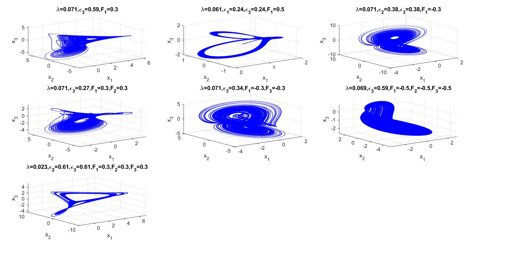
Figure 1: Orbits of chaotic cases for subclass $1$ with $p+q+r\neq 0$: having nonzero $\left(F_{1},\epsilon_{3}\right)$, $\left(F_{1},\epsilon_{1},\epsilon_{3}\right)$, $\left(F_{1},\epsilon_{2},\epsilon_{3}\right)$, $\left(F_{1},F_{2},\epsilon_{3}\right)$, $\left(F_{1},F_{3},\epsilon_{3}\right)$, $\left(F_{1},F_{2},F_{3},\epsilon_{3}\right)$ and $\left(F_{1},F_{2},F_{3},\epsilon_{2},\epsilon_{3}\right)$. Each of these has nonzero $\left(F_{1},\epsilon_{3}\right)$, the MCM for subclass $1$.

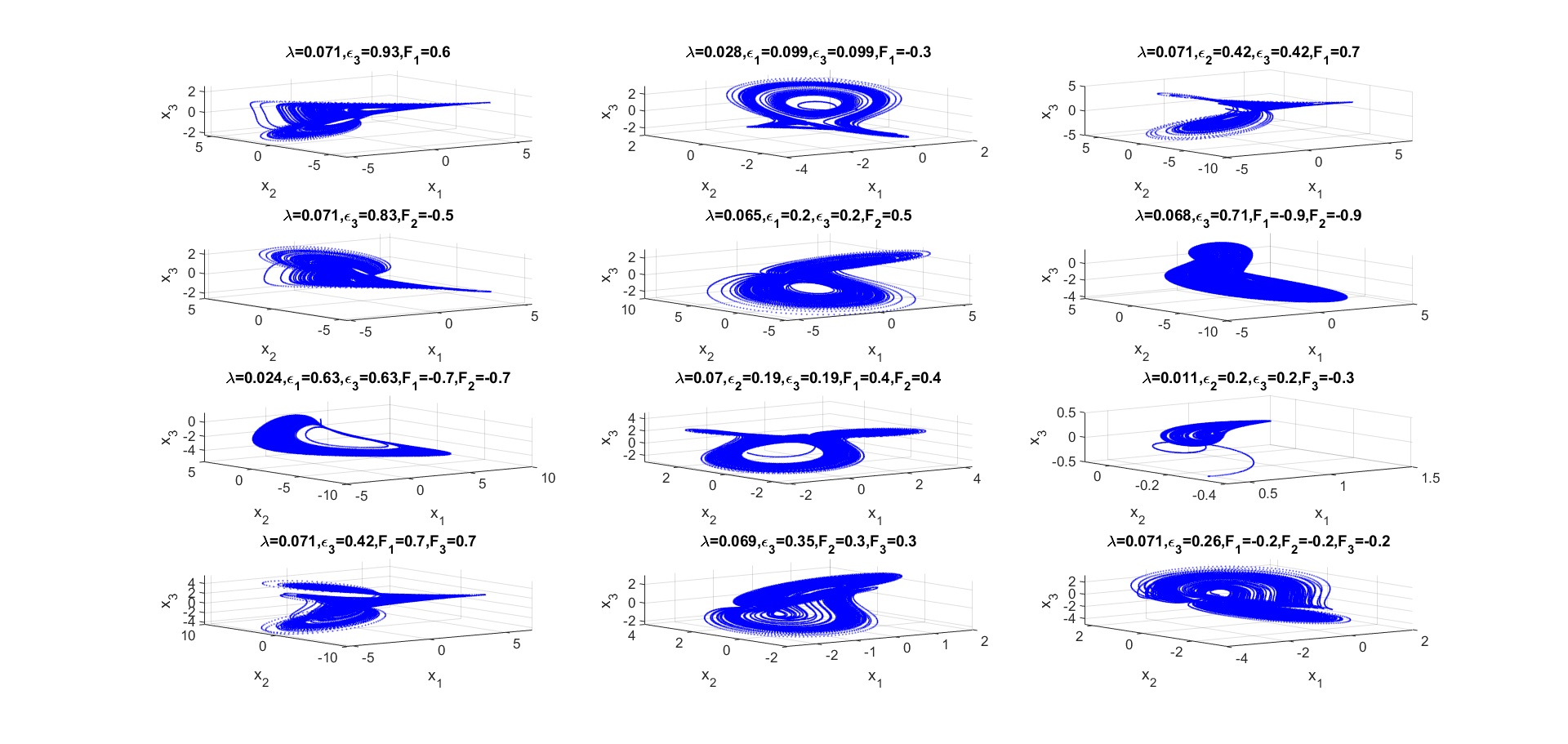
Figure 2: Orbits of chaotic cases for subclass $2$ with $p+q+r\neq 0$: having nonzero $\left(F_{1},\epsilon_{3}\right)$, $\left(F_{1},\epsilon_{1},\epsilon_{3}\right)$, $\left(F_{1},\epsilon_{2},\epsilon_{3}\right)$, $\left(F_{2},\epsilon_{3}\right)$, $\left(F_{2},\epsilon_{1},\epsilon_{3}\right)$, $\left(F_{1},F_{2},\epsilon_{3}\right)$, $\left(F_{1},F_{2},\epsilon_{1},\epsilon_{3}\right)$, $\left(F_{1},F_{2},\epsilon_{2},\epsilon_{3}\right)$, $\left(F_{3},\epsilon_{2},\epsilon_{3}\right)$, $\left(F_{1},F_{3},\epsilon_{3}\right)$, $\left(F_{2},F_{3},\epsilon_{3}\right)$ and $\left(F_{1},F_{2},F_{3},\epsilon_{3}\right)$. The simplest chaotic cases, having one forcing and one dissipation term, involve nonzero $\left(F_{1},\epsilon_{3}\right)$ and $\left(F_{2},\epsilon_{3}\right)$. Together with $\left(F_{3},\epsilon_{2},\epsilon_{3}\right)$, which is irreducible, there are $3$ MCMs for subclass $2$.

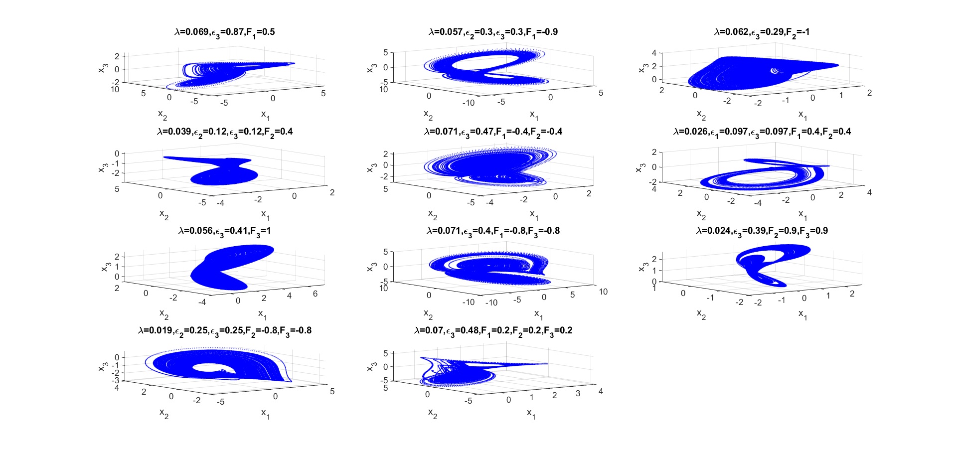
Figure 3: Orbits of chaotic cases for subclass $3$ with $p+q+r\neq 0$: having nonzero $\left(F_{1},\epsilon_{3}\right)$, $\left(F_{1},\epsilon_{2},\epsilon_{3}\right)$, $\left(F_{2},\epsilon_{3}\right)$, $\left(F_{2},\epsilon_{2},\epsilon_{3}\right)$, $\left(F_{1},F_{2},\epsilon_{3}\right)$, $\left(F_{1},F_{2},\epsilon_{1},\epsilon_{3}\right)$, $\left(F_{3},\epsilon_{3}\right)$, $\left(F_{1},F_{3},\epsilon_{3}\right)$, $\left(F_{2},F_{3},\epsilon_{3}\right)$, $\left(F_{2},F_{3},\epsilon_{2},\epsilon_{3}\right)$ and $\left(F_{1},F_{2},F_{3},\epsilon_{3}\right)$. The simplest chaotic cases, having one forcing and one dissipation term, involve nonzero $\left(F_{1},\epsilon_{3}\right)$, $\left(F_{2},\epsilon_{3}\right)$, and $\left(F_{3},\epsilon_{3}\right)$. Each of the chaotic cases can be reduced to one of these, by setting some terms to zero, and hence there are $3$ MCMs with nonzero $\left(F_{1},\epsilon_{3}\right)$, $\left(F_{2},\epsilon_{3}\right)$, and $\left(F_{3},\epsilon_{3}\right)$ for subclass $3$.

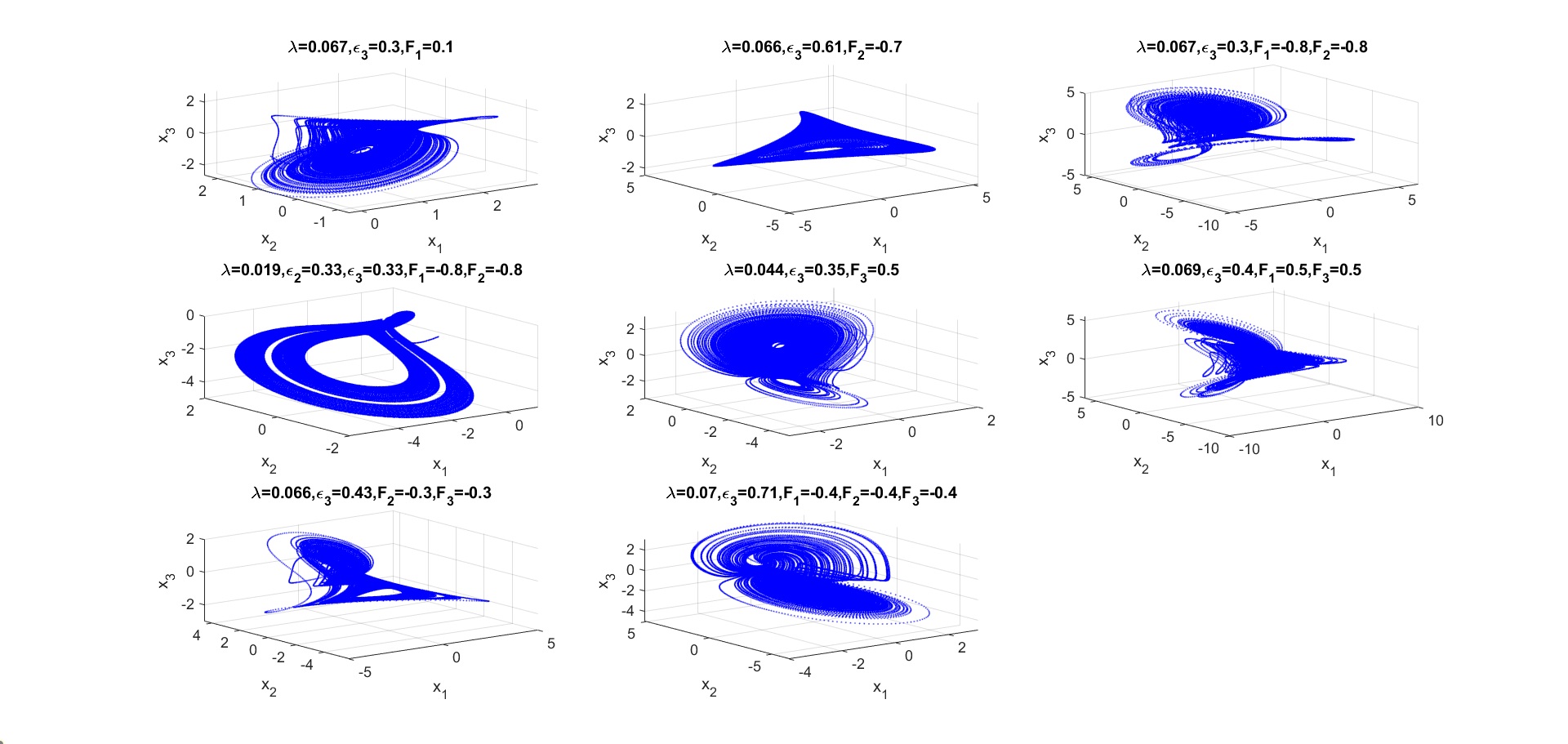
Figure 4: Orbits of chaotic cases for subclass $4$ with $p+q+r\neq 0$: having nonzero $\left(F_{1},\epsilon_{3}\right)$, $\left(F_{2},\epsilon_{3}\right)$, $\left(F_{1},F_{2},\epsilon_{3}\right)$, $\left(F_{1},F_{2},\epsilon_{2},\epsilon_{3}\right)$, $\left(F_{3},\epsilon_{3}\right)$, $\left(F_{1},F_{3},\epsilon_{3}\right)$, $\left(F_{2},F_{3},\epsilon_{3}\right)$ and $\left(F_{1},F_{2},F_{3},\epsilon_{3}\right)$. The simplest chaotic cases, having one forcing and one dissipation term, involve nonzero $\left(F_{1},\epsilon_{3}\right)$, $\left(F_{2},\epsilon_{3}\right)$, and $\left(F_{3},\epsilon_{3}\right)$. Each of the chaotic cases can be reduced to one of these, by setting some terms to zero, and hence there are $3$ MCMs with nonzero $\left(F_{1},\epsilon_{3}\right)$, $\left(F_{2},\epsilon_{3}\right)$, and $\left(F_{3},\epsilon_{3}\right)$ for subclass $4$.

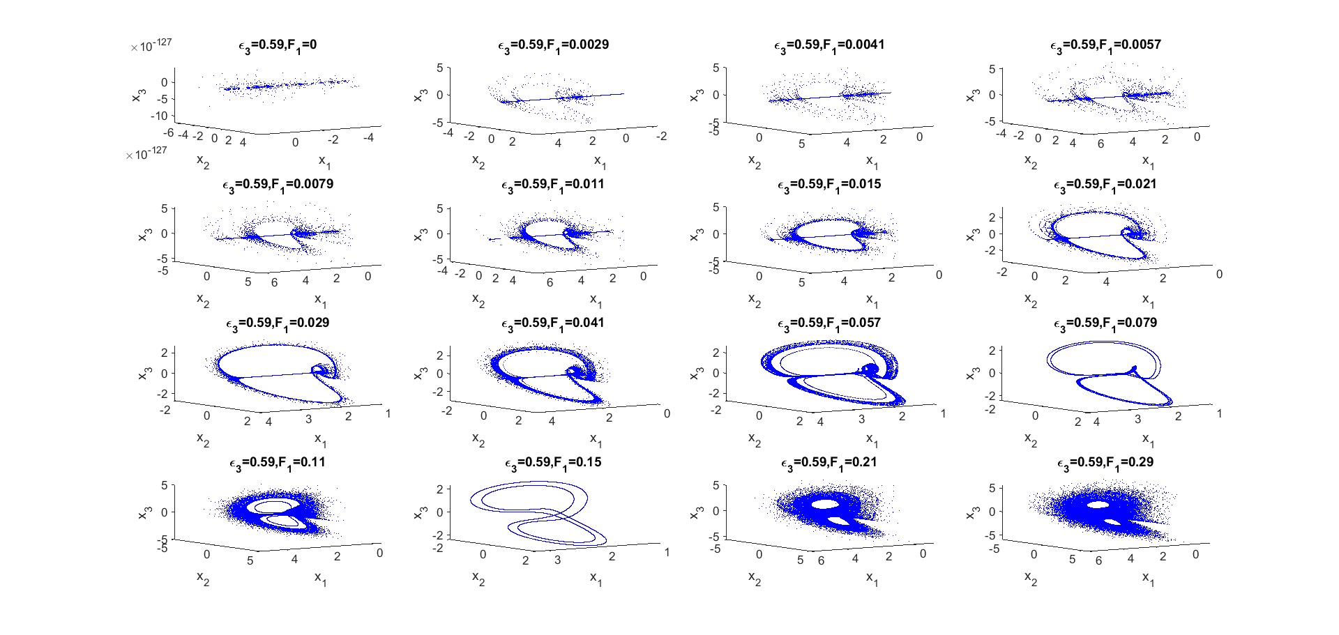
Figure 5: Orbits of the MCM $\left(F_{1},\epsilon_{3}\right)$ of subclass $1$, as the forcing is increased from $0$, for a large initial condition ensemble. The case with $F_{1}=0.021$ is considered further in Figure 8.

For subclass 1 there are many cases with positive LLE ($17$ have been found explicitly; see Supplementary Information (SI) Figures 1-5), but only some of these are chaotic by the various measures examined. The chaotic cases have nonzero $\left(F_{1},\epsilon_{3}\right)$, $\left(F_{1},\epsilon_{1},\epsilon_{3}\right)$, $\left(F_{1},\epsilon_{2},\epsilon_{3}\right)$, $\left(F_{1},F_{2},\epsilon_{3}\right)$, $\left(F_{1},F_{3},\epsilon_{3}\right)$, $\left(F_{1},F_{2},F_{3},\epsilon_{3}\right)$ and $\left(F_{1},F_{2},F_{3},\epsilon_{2},\epsilon_{3}\right)$. Despite the diversity of chaotic orbits (Figure 1), inspection identifies a unique MCM with nonzero $\left(F_{1},\epsilon_{3}\right)$, since each of these cases has nonzero $F_{1}$ and $\epsilon_{3}$. For each case the most chaotic version of the $2000$-member ensemble, having the largest positive value of LLE, has been plotted to illustrate the appearance of chaos (Figure 1).

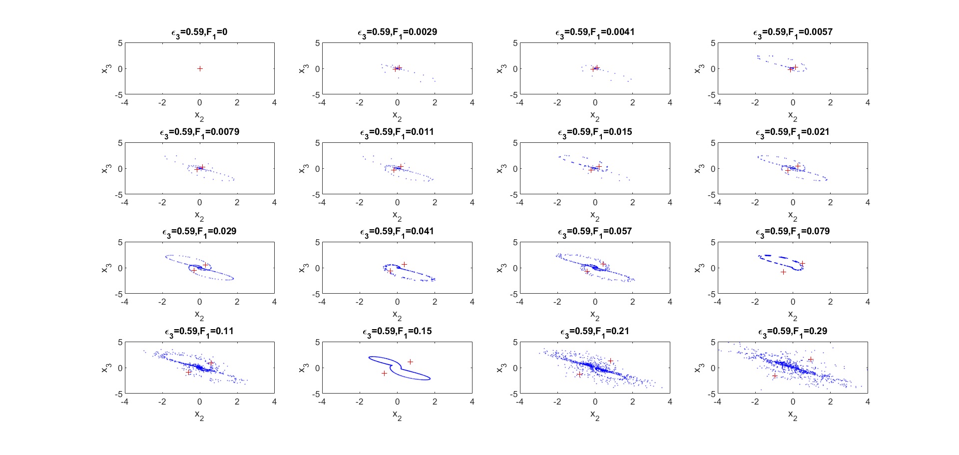
Figure 6: Orbits of MCM $\left(F_{1},\epsilon_{3}\right)$ of subclass $1$ in Figure 5 projected onto the $x_{2}-x_{3}$ plane. Red crosses indicate the fixed points.

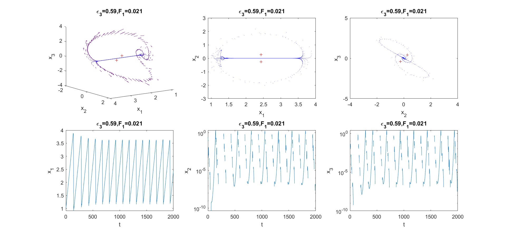
Figure 8: Orbit of MCM $\left(F_{1},\epsilon_{3}\right)$ for subclass $1$, for $F_{1}=0.021$ and the initial condition $\left(1,0.2,0.2\right)$. Arrows indicate the direction of the vector field along the orbit. Also shown are corresponding $2-$dimensional projections, and time-series. The logarithmic scale for the time-series of $x_{2}$ and $x_{3}$ illustrates breaks in the curve where the sign is negative, and the orbit never reaches the invariant set $x_{2}=0,x_{3}=0$. Thus, the orbit exhibits oscillatory behavior around points on the invariant set, which eventually becomes unstable as $x_{1}$ increases. There is no fixed point along this invariant set, and thus no homoclinic orbits. The model parameters are $a=-0.94$, $p=0.19$, and $q=-0.39$.

Similarly, for subclass $2$, of the $23$ cases with positive LLE (SI Figures 6-10), there are $12$ cases that are chaotic by all the measures in Section 2. These cases (orbits in Figure 2), have nonzero $\left(F_{1},\epsilon_{3}\right)$,$\left(F_{1},\epsilon_{1},\epsilon_{3}\right)$,$\left(F_{1},\epsilon_{2},\epsilon_{3}\right)$, $\left(F_{2},\epsilon_{3}\right)$,$\left(F_{2},\epsilon_{1},\epsilon_{3}\right)$,$\left(F_{1},F_{2},\epsilon_{3}\right)$,$\left(F_{1},F_{2},\epsilon_{1},\epsilon_{3}\right)$ ,$\left(F_{1},F_{2},\epsilon_{2},\epsilon_{3}\right),\left(F_{3},\epsilon_{2},\epsilon_{3}\right),\left(F_{1},F_{3},\epsilon_{3}\right)$,$\left(F_{2},F_{3},\epsilon_{3}\right)$ and $\left(F_{1},F_{2},F_{3},\epsilon_{3}\right)$. The MCMs as defined above include all proper subsets, and not only those that have the fewest number of terms. The simplest such MCMs, with one forcing and one dissipation term, involve nonzero $\left(F_{1},\epsilon_{3}\right)$ and $\left(F_{2},\epsilon_{3}\right)$. In addition, there is nonzero $\left(F_{3},\epsilon_{2},\epsilon_{3}\right)$, which is irreducible to the other two MCMs owing to different placement of forcing. Thus there are $3$ MCMs for subclass $2$: $\left(F_{1},\epsilon_{3}\right)$, $\left(F_{2},\epsilon_{3}\right)$, and $\left(F_{3},\epsilon_{2},\epsilon_{3}\right)$, for $p+q+r\neq 0$.

Similar analysis for subclasses $3$ and $4$ identifies $11$ and $8$ chaotic cases respectively, whose orbits are shown in Figures 3–4. For both of these subclasses, there are $3$ MCMs, with nonzero $\left(F_{1},\epsilon_{3}\right)$, $\left(F_{2},\epsilon_{3}\right)$, and $\left(F_{3},\epsilon_{3}\right)$. The corresponding time-series of $x_{1}$, Poincar$\acute{\textrm{e}}$ sections, power spectra of the stationary orbits, and evolution of LLE, are shown in SI Figures 11-14, and Figures 15-18, respectively for the two subclasses.

Table 1 below summarizes the chaotic cases and MCMs, for each of the subclasses. It lists each of the chaotic cases for subclasses 1-4, identified by the multiple lines of evidence (Section 2), and inspection of these cases identifies the MCMs. While siting of forcing can vary between subclasses, the most basic condition on dissipation is the same and all chaotic cases must involve dissipation in the third (i.e., linear) equation through nonzero $\epsilon_{3}$.

With energy conservation constraint, i.e., $p+q+r=0$:

Table 1 also lists the MCMs when the energy conservation constraint is present, based on simulations with $q=-p$, since $r=0$. This is based on a complete listing of cases with positive LLEs (SI Figures 22-24, 25-27, 28-30, and 31-33 for subclasses $1-4$ respectively), for which we have used the aforementioned criteria to identify chaotic cases and thereby establish MCMs. Table 1 below shows that generally there are fewer MCMs when energy is conserved.

For subclass $1$, there is no effect of the energy conservation constraint, with MCM $\left(F_{1},\epsilon_{3}\right)$ in either case.

In subclass $2$, only $\left(F_{1},\epsilon_{3}\right)$ and $\left(F_{2},\epsilon_{3}\right)$ are MCMs when energy is conserved.

For subclass $3$, $\left(F_{1},\epsilon_{3}\right)$ is an MCM while $\left(F_{2},\epsilon_{3}\right)$ and $\left(F_{3},\epsilon_{3}\right)$ are not.

Similarly, in subclass $4$, $\left(F_{1},\epsilon_{3}\right)$ and $\left(F_{2},\epsilon_{3}\right)$ are MCMs, while $\left(F_{3},\epsilon_{3}\right)$ is not.

If the gyrostat core conserves energy, forcing can be placed in fewer ways for the model to admit chaos. These effects of the energy conservation constraint on the MCMs are explained in the following section. When energy is conserved in the gyrostat core, the MCMs are governed by the arrangement of fixed points $\left(x_{1}^{*},x_{2}^{*},x_{3}^{*}\right)$ in the model with F&D. For each subclass, the resulting conditions for MCMs are found by inspecting the cubic equation for $x_{3}^{*}$, whose coefficients are shown in the last column of Table 1. This is because chaos for the energy conserving case requires a pair of fixed points with opposite signs of $x_{3}^{*}$.

Table 1: Chaotic cases, minimal chaotic models (MCMs), and coefficients of cubic equation describing $x_{3}^{*}$ for subclasses $1-4$.

Subclass	Chaotic cases $\left(p+q+r\neq 0\right)$	MCM $\left(p+q+r\neq 0\right)$	MCM $\left(p+q+r=0\right)$	Coefficients of cubic equation for $x_{3}^{*}$
$1$	$\left(F_{1},\epsilon_{3}\right)$, $\left(F_{1},\epsilon_{1},\epsilon_{3}\right)$, $\left(F_{1},\epsilon_{2},\epsilon_{3}\right)$,	$\left(F_{1},\epsilon_{3}\right)$	$\left(F_{1},\epsilon_{3}\right)$	$\gamma_{3}=\epsilon_{3}\frac{p}{a}$
	$\left(F_{1},F_{2},\epsilon_{3}\right)$, $\left(F_{1},F_{3},\epsilon_{3}\right)$,			$\gamma_{2}=-F_{3}\frac{p}{a}$,
	$\left(F_{1},F_{2},F_{3},\epsilon_{3}\right)$,			$\gamma_{1}=F_{1}-\epsilon_{1}\frac{a}{q}-\epsilon_{1}\epsilon_{2}\epsilon_{3}\frac{1}{aq}$,
	$\left(F_{1},F_{2},F_{3},\epsilon_{2},\epsilon_{3}\right)$.			$\gamma_{0}=\frac{F_{2}\epsilon_{1}}{q}+\frac{F_{3}\epsilon_{1}\epsilon_{2}}{aq}$.
$2$	$\left(F_{1},\epsilon_{3}\right)$, $\left(F_{1},\epsilon_{1},\epsilon_{3}\right)$, $\left(F_{1},\epsilon_{2},\epsilon_{3}\right)$,	$\left(F_{1},\epsilon_{3}\right),$$\left(F_{2},\epsilon_{3}\right)$,$\left(F_{3},\epsilon_{2},\epsilon_{3}\right)$	$\left(F_{1},\epsilon_{3}\right),$$\left(F_{2},\epsilon_{3}\right)$	$\gamma_{3}=\epsilon_{3}\frac{p}{a}$,
	$\left(F_{2},\epsilon_{3}\right)$, $\left(F_{2},\epsilon_{1},\epsilon_{3}\right)$,$\left(F_{1},F_{2},\epsilon_{3}\right)$,			$\gamma_{2}=-F_{3}\frac{p}{a}+b\left(1+\frac{p}{q}\right)$,
	$\left(F_{1},F_{2},\epsilon_{1},\epsilon_{3}\right)$,$\left(F_{1},F_{2},\epsilon_{2},\epsilon_{3}\right),\left(F_{3},\epsilon_{2},\epsilon_{3}\right),$			$\gamma_{1}=F_{1}-F_{2}b\frac{p}{aq}-\epsilon_{1}\frac{a}{q}-\epsilon_{1}\epsilon_{2}\epsilon_{3}\frac{1}{aq}-\epsilon_{2}\frac{b^{2}}{aq}$,
	$\left(F_{1},F_{3},\epsilon_{3}\right)$, $\left(F_{2},F_{3},\epsilon_{3}\right)$, $\left(F_{1},F_{2},F_{3},\epsilon_{3}\right)$.			$\gamma_{0}=\frac{F_{2}\epsilon_{1}}{q}+\frac{F_{3}\epsilon_{1}\epsilon_{2}}{aq}-F_{1}\epsilon_{2}\frac{b}{aq}$.
$3$	$\left(F_{1},\epsilon_{3}\right)$, $\left(F_{1},\epsilon_{2},\epsilon_{3}\right)$, $\left(F_{2},\epsilon_{3}\right)$,	$\left(F_{1},\epsilon_{3}\right)$, $\left(F_{2},\epsilon_{3}\right)$, $\left(F_{3},\epsilon_{3}\right)$	$\left(F_{1},\epsilon_{3}\right)$	$\gamma_{3}=\epsilon_{3}\frac{p}{a}$,
	$\left(F_{2},\epsilon_{2},\epsilon_{3}\right)$,$\left(F_{1},F_{2},\epsilon_{3}\right)$,			$\gamma_{2}=-F_{3}\frac{p}{a}+\epsilon_{3}\frac{c}{a}\left(\frac{p}{q}-1\right)$,
	$\left(F_{1},F_{2},\epsilon_{1},\epsilon_{3}\right)$,$\left(F_{3},\epsilon_{3}\right),\left(F_{1},F_{3},\epsilon_{3}\right)$,			$\gamma_{1}=F_{1}-F_{3}\frac{c}{a}\left(\frac{p}{q}-1\right)-\epsilon_{1}\frac{a}{q}-\epsilon_{1}\epsilon_{2}\epsilon_{3}\frac{1}{aq}-\epsilon_{3}\frac{c^{2}}{aq}$,
	$\left(F_{2},F_{3},\epsilon_{3}\right)$, $\left(F_{2},F_{3},\epsilon_{2},\epsilon_{3}\right)$, $\left(F_{1},F_{2},F_{3},\epsilon_{3}\right)$.			$\gamma_{0}=F_{1}\frac{c}{q}+\frac{F_{2}\epsilon_{1}}{q}+F_{3}\left(\frac{c^{2}}{aq}+\frac{\epsilon_{1}\epsilon_{2}}{aq}\right)$.
$4$	$\left(F_{1},\epsilon_{3}\right)$, $\left(F_{2},\epsilon_{3}\right)$, $\left(F_{1},F_{2},\epsilon_{3}\right)$,	$\left(F_{1},\epsilon_{3}\right)$, $\left(F_{2},\epsilon_{3}\right)$, $\left(F_{3},\epsilon_{3}\right)$	$\left(F_{1},\epsilon_{3}\right)$, $\left(F_{2},\epsilon_{3}\right)$	$\gamma_{3}=\epsilon_{3}\frac{p}{a}$
	$\left(F_{1},F_{2},\epsilon_{2},\epsilon_{3}\right)$,$\left(F_{3},\epsilon_{3}\right),\left(F_{1},F_{3},\epsilon_{3}\right)$,			$\gamma_{2}=-F_{3}\frac{p}{a}+\epsilon_{3}\frac{c}{a}\left(\frac{p}{q}-1\right)+b\left(1+\frac{px_{1}^{*}}{a}\right)$,
	$\left(F_{2},F_{3},\epsilon_{3}\right)$, $\left(F_{1},F_{2},F_{3},\epsilon_{3}\right)$.			$\gamma_{1}=F_{1}-F_{3}\frac{c}{a}\left(\frac{p}{q}-1\right)-\epsilon_{1}\frac{a}{q}-\epsilon_{1}\epsilon_{2}\epsilon_{3}\frac{1}{aq}-\epsilon_{3}\frac{c^{2}}{aq}+\frac{bc}{q}+\frac{bcx_{1}^{*}}{a}\left(\frac{p}{q}-1\right)$,
				$\gamma_{0}=F_{1}\frac{c}{q}+\frac{F_{2}\epsilon_{1}}{q}+F_{3}\left(\frac{c^{2}}{aq}+\frac{\epsilon_{1}\epsilon_{2}}{aq}\right)-\frac{bx_{1}^{*}\left(c^{2}+\epsilon_{1}\epsilon_{2}\right)}{aq}$.

4 Accounting for minimal chaotic models

4.1 Subclass 1 with $r=0,b=c=0$

This subclass of the Volterra gyrostat has evolution

$$x_{1}^{\prime} =px_{2}x_{3}$$

$$x_{2}^{\prime} =qx_{3}x_{1}-ax_{3}.$$

$$x_{3}^{\prime} =ax_{2}$$ (5)

and serves as the conservative core of many important LOMs (Gluhovsky and Tong (1999)), including that of Lorenz (1963). It has two invariants irrespective of whether $p+q=0$ (Seshadri and Lakshmivarahan (2023)), and rotational symmetry $R_{x_{1}}\left(\pi\right)$ about the axis of $x_{1}$, i.e. the equations are preserved under the transformation $\left(x_{1},x_{2},x_{3}\right)\rightarrow\left(x_{1},-x_{2},-x_{3}\right)$. All chaotic cases have nonzero $\left(F_{1},\epsilon_{3}\right)$ and the MCM

$$x_{1}^{\prime} =px_{2}x_{3}+F_{1}$$

$$x_{2}^{\prime} =qx_{3}x_{1}-ax_{3}.$$

$$x_{3}^{\prime} =ax_{2}-\epsilon_{3}x_{3}$$ (6)

maintains the symmetry $R_{x_{1}}\left(\pi\right)$. For this last system there are two distinct fixed points given by $\left(a/q,x_{2}^{*},x_{3}^{*}\right)$ and $\left(a/q,-x_{2}^{*},-x_{3}^{*}\right)$ with $x_{2}^{*2}=-\frac{\epsilon_{3}F_{1}}{ap}$ and $x_{3}^{*2}=-\frac{aF_{1}}{p\epsilon_{3}}$, which are real if $F_{1}$ has opposite sign from $ap$ $\left(\epsilon_{3}>0\right)$. The Jacobian evaluated at $\left(a/q,x_{2}^{*},x_{3}^{*}\right)$ becomes

$$\mathrm{D}_{\mathrm{f}}=\left[\begin{array}[]{ccc}0&px_{3}^{*}&px_{2}^{*}\\ qx_{3}^{*}&0&0\\ 0&a&-\epsilon_{3}\end{array}\right]$$ (7)

having characteristic polynomial

$$\lambda^{3}+\epsilon_{3}\lambda^{2}-pqx_{3}^{*2}\lambda-2\epsilon_{3}pqx_{3}^{*2}=0,$$ (8)

where we have used, from the last component of Eq. (6), $x_{2}^{*}=\left(\epsilon_{3}/a\right)x_{3}^{*}$. From the symmetry of the equations, the Jacobian evaluated at $\left(a/q,-x_{2}^{*},-x_{3}^{*}\right)$ also has the same characteristic polynomial, and thus the above fixed points make a pair with identical stability. Moreover the discriminant of the characteristic polynomial in Eq. (8) is negative

$$\Delta=pqx_{3}^{*2}\left(8\epsilon_{3}^{4}-71\epsilon_{3}^{2}pqx_{3}^{*2}+4p^{2}q^{2}x_{3}^{*4}\right)<0$$ (9)

in case $pq<0$, since $x_{3}^{*2}>0$. The MCM plotted in Figure 1 has parameters $a=-0.94$, $p=0.19$, and $q=-0.39$, so that indeed $pq<0$. Therefore there are two complex eigenvalues at each fixed point, with a Hopf bifurcation occurring when the real part crosses the imaginary axis. With product of all eigenvalues being negative there is one stable direction, but with large $F_{1}$ the real part of the complex conjugate pair becomes positive and the fixed points repel nearby trajectories.

These properties are not maintained in case a single forcing and dissipation term occur elsewhere. Table 2 lists the $8$ alternate ways in which a single forcing and a single dissipation term can be placed. None of these can admit chaos. Each of these yields a different arrangement of fixed points from the above: ranging from no fixed points to an entire line. Where a pair of fixed points exists, they do not possess the above symmetry. The MCM $\left(F_{1},\epsilon_{3}\right)$ is not alone in maintaining the symmetry of the gyrostat core, and other non-chaotic cases in Table 2, such as $\left(F_{1},\epsilon_{1}\right)$ and $\left(F_{1},\epsilon_{2}\right)$, maintain it as well. The MCM $\left(F_{1},\epsilon_{3}\right)$ has the unique attribute of maintaining symmetry of the equations while giving rise to a pair of distinct and symmetrically placed fixed points with opposite signs of $x_{3}^{*}$. Other chaotic cases listed in Table 1 do not always maintain this symmetry. As shown below, the necessary condition for appearance of chaos in this subclass is a pair of fixed points arranged on opposite sides of the $x_{1}-x_{2}$ plane. The MCM $\left(F_{1},\epsilon_{3}\right)$ also appears when energy is conserved in the gyrostat core (SI Figs. 22-24; Table 1).

Table 2: Fixed points for various other placements of one F&D term (besides the MCM) in Subclass 1.

S. No	Model	Equations	Fixed Points
$1$	$F_{1},\epsilon_{1}$	$x_{1}^{\prime}=px_{2}x_{3}+F_{1}-\epsilon_{1}x_{1}\textrm{, }x_{2}^{\prime}=qx_{3}x_{1}-ax_{3}\textrm{, }x_{3}^{\prime}=ax_{2}$	$\left(\frac{F_{1}}{\epsilon_{1}},0,0\right)$
$2$	$F_{1},\epsilon_{2}$	$x_{1}^{\prime}=px_{2}x_{3}+F_{1}\textrm{, }x_{2}^{\prime}=qx_{3}x_{1}-ax_{3}-\epsilon_{2}x_{2}\textrm{, }x_{3}^{\prime}=ax_{2}$	None
$3$	$F_{2},\epsilon_{1}$	$x_{1}^{\prime}=px_{2}x_{3}-\epsilon_{1}x_{1}\textrm{, }x_{2}^{\prime}=qx_{3}x_{1}-ax_{3}+F_{2}\textrm{, }x_{3}^{\prime}=ax_{2}$	$\left(0,0,\frac{F_{2}}{a}\right)$
$4$	$F_{2},\epsilon_{2}$	$x_{1}^{\prime}=px_{2}x_{3}\textrm{, }x_{2}^{\prime}=qx_{3}x_{1}-ax_{3}+F_{2}-\epsilon_{2}x_{2}\textrm{, }x_{3}^{\prime}=ax_{2}$	$\left(x_{1}^{*},0,-\frac{F_{2}}{qx_{1}^{*}-a}\right)$
$5$	$F_{2},\epsilon_{3}$	$x_{1}^{\prime}=px_{2}x_{3}\textrm{, }x_{2}^{\prime}=qx_{3}x_{1}-ax_{3}+F_{2}\textrm{, }x_{3}^{\prime}=ax_{2}-\epsilon_{3}x_{3}$	None
$6$	$F_{3},\epsilon_{1}$	$x_{1}^{\prime}=px_{2}x_{3}-\epsilon_{1}x_{1}\textrm{, }x_{2}^{\prime}=qx_{3}x_{1}-ax_{3}\textrm{, }x_{3}^{\prime}=ax_{2}+F_{3}$	$\left(0,-\frac{F_{3}}{a},0\right)$ and $\left(\frac{a}{q},-\frac{F_{3}}{a},-\frac{\epsilon_{1}a^{2}}{pqF_{3}}\right)$
$7$	$F_{3},\epsilon_{2}$	$x_{1}^{\prime}=px_{2}x_{3}\textrm{, }x_{2}^{\prime}=qx_{3}x_{1}-ax_{3}-\epsilon_{2}x_{2}\textrm{, }x_{3}^{\prime}=ax_{2}+F_{3}$	None
$8$	$F_{3},\epsilon_{3}$	$x_{1}^{\prime}=px_{2}x_{3}\textrm{, }x_{2}^{\prime}=qx_{3}x_{1}-ax_{3}\textrm{, }x_{3}^{\prime}=ax_{2}+F_{3}-\epsilon_{3}x_{3}$	$\left(\frac{a}{q},0,\frac{F_{3}}{\epsilon_{3}}\right)$ and $\left(x_{1}^{*},-\frac{F_{3}}{a},0\right)$

More generally, this subclass with F&D

$$x_{1}^{\prime} =px_{2}x_{3}-\epsilon_{1}x_{1}+F_{1}$$

$$x_{2}^{\prime} =qx_{3}x_{1}-ax_{3}-\epsilon_{2}x_{2}+F_{2}$$

$$x_{3}^{\prime} =ax_{2}-\epsilon_{3}x_{3}+F_{3}$$ (10)

has fixed points $\left(x_{1}^{*},x_{2}^{*},x_{3}^{*}\right)$ as follows: from the third equation, $x_{2}^{*}=-\left(F_{3}-\epsilon_{3}x_{3}^{*}\right)/a$ and from the second equation $qx_{1}^{*}x_{3}^{*}=ax_{3}^{*}+\epsilon_{2}x_{2}^{*}-F_{2}$. Together these equations must obey consistency

$$\left(qx_{1}^{*}-\frac{\epsilon_{2}\epsilon_{3}}{a}-a\right)x_{3}^{*}=-\frac{F_{3}\epsilon_{2}}{a}-F_{2}$$ (11)

so that when $x_{3}^{*}=0$ the right hand side of Eq. (11) must also vanish. A second consistency condition is furnished by the first equation

$$px_{2}^{*}x_{3}^{*}=-F_{1}+\epsilon_{1}x_{1}^{*}$$ (12)

so that zero $x_{3}^{*}$ in conjunction with nonzero $F_{1}$ also entails nonzero $\epsilon_{1}$. These consistency conditions are met by the cases illustrated in Table 1. Using these relations to eliminate $x_{1}^{*},x_{2}^{*}$ from the first equation we obtain a cubic in $x_{3}^{*}$

$$\gamma_{3}x_{3}^{*3}+\gamma_{2}x_{3}^{*2}+\gamma_{1}x_{3}^{*}+\gamma_{0} =0$$ (13)

where

$$\gamma_{3} =\epsilon_{3}\frac{p}{a},$$

$$\gamma_{2} =-F_{3}\frac{p}{a},$$

$$\gamma_{1} =F_{1}-\epsilon_{1}\frac{a}{q}-\epsilon_{1}\epsilon_{2}\epsilon_{3}\frac{1}{aq},$$

$$\gamma_{0} =\frac{F_{2}\epsilon_{1}}{q}+\frac{F_{3}\epsilon_{1}\epsilon_{2}}{aq}.$$ (14)

The number and arrangement of fixed points depends on the number of real roots of Eq. (13), subject to the two consistency conditions. Recall that the MCM has nonzero $\left(F_{1},\epsilon_{3}\right)$. The resulting expression becomes

$$\epsilon_{3}\frac{p}{a}x_{3}^{*3}+F_{1}x_{3}^{*}=0$$ (15)

yielding two roots satisfying $x_{3}^{*2}=-\frac{aF_{1}}{p\epsilon_{3}}$ as found above. This is a simple model with F&D yielding two fixed points with positive and negative $x_{3}^{*}$. In fact, the MCM $\left(F_{1},\epsilon_{3}\right)$ provides the simplest model giving a pair of fixed points, with opposite signs of $x_{3}^{*}$, which can undergo a Hopf bifurcation.

Such fixed points play an important role in the Lorenz model (Sparrow (1982)). On the route to chaos, as the forcing is increased, following the Hopf bifurcation, trajectories spiral around these unstable fixed points at an increasing distance (Kaplan and Yorke (1979)). For subclass $1$, the existence of this pair is central to the MCM.

There is an important difference with the Lorenz model, which must be pointed out: the absence of a third fixed point, a saddle, for the MCM precludes homoclinic orbits that are important in the Lorenz model’s dynamics (Sparrow (1982)). Despite this, chaos arises on account of the pair of fixed points, with positive/negative $x_{3}^{*}$, yielding opposing spirals when projected onto the $x_{1}-x_{2}$ plane.

4.2 Subclass 2 with $r=0,c=0$

Here the conservative core

$$x_{1}^{\prime} =px_{2}x_{3}+bx_{3}$$

$$x_{2}^{\prime} =qx_{3}x_{1}-ax_{3}$$

$$x_{3}^{\prime} =ax_{2}-bx_{1}$$ (16)

has a single invariant (Seshadri and Lakshmivarahan (2023)) in general with $p+q\neq 0$, and, compared to subclass $1$, $b\neq 0$ breaks the symmetry $R_{x_{1}}\left(\pi\right)$. The MCMs $\left(F_{1},\epsilon_{3}\right)$ and $\left(F_{2},\epsilon_{3}\right)$, which both appear even with $p+q+r=0$ (Table 1), are analogous, so we consider $\left(F_{1},\epsilon_{3}\right)$

$$x_{1}^{\prime} =px_{2}x_{3}+bx_{3}+F_{1}$$

$$x_{2}^{\prime} =qx_{3}x_{1}-ax_{3}$$

$$x_{3}^{\prime} =ax_{2}-bx_{1}-\epsilon_{3}x_{3}$$ (17)

whose fixed points are given by $\left(\frac{a}{q},\frac{b}{q}+\frac{\epsilon_{3}}{a}x_{3}^{*},x_{3}^{*}\right)$ where $x_{3}^{*}$ solves the quadratic equation $\epsilon_{3}pqx_{3}^{*2}+ab\left(p+q\right)x_{3}^{*}+aqF_{1}=0$. The Jacobian evaluated at the fixed point

$$\mathrm{D}_{\mathrm{f}}=\left[\begin{array}[]{ccc}0&px_{3}^{*}&px_{2}^{*}+b\\ qx_{3}^{*}&0&0\\ -b&a&-\epsilon_{3}\end{array}\right]$$ (18)

has eigenvalues solving characteristic polynomial

$$\lambda^{3}+\epsilon_{3}\lambda^{2}-\left(pqx_{3}^{*2}-b\right)\lambda-\epsilon_{3}pqx_{3}^{*2}+aqF_{1}=0,$$ (19)

which depends on $x_{3}^{*2}$. For $p+q\neq 0$ the two fixed points do not have identical stability. As with subclass $1$, for $F_{1}$ sufficiently large the complex eigenvalues have positive real part so this pair of fixed points repels the flow in the neighborhoods. The key condition for these MCMs is, again, the pair of fixed points with opposite signs of $x_{3}^{*}$.

In contrast, the other MCM $\left(F_{3},\epsilon_{2},\epsilon_{3}\right)$

$$x_{1}^{\prime} =px_{2}x_{3}+bx_{3}$$

$$x_{2}^{\prime} =qx_{3}x_{1}-ax_{3}-\epsilon_{2}x_{2}$$

$$x_{3}^{\prime} =ax_{2}-bx_{1}-\epsilon_{3}x_{3}+F_{3}$$ (20)

does not appear in the presence of energy conservation, and cannot be rooted in the aforementioned property of fixed points, which does not hold (as shown below).

Therefore, with the energy conservation constraint, let us examine the $7$ alternate placements of a single forcing and dissipation term in Table 3. Most of the alternate placements yield only a single fixed point, whereas those with two fixed points have one of them lying on the $x_{1}-x_{2}$ plane. This does not favor the pair of opposing spirals described above. Only the MCMs $\left(F_{1},\epsilon_{3}\right)$ and $\left(F_{2},\epsilon_{3}\right)$ lead to a pair of fixed points with opposite signs of $x_{3}^{*}$, and these are the ones leading to the pair of opposing spirals (see Eq. (18)). It is therefore not surprising that these are the MCMs obtained with $p+q+r=0$ (SI Figs. 25-27; Table 1). In summary, with the energy conservation constraint in the gyrostat core, the requirement of a pair of fixed points with opposite $x_{3}^{*}$ circumscribes the MCMs.

Table 3: Fixed points for various other placements of one forcing and dissipation term in Subclass 2. Here we have taken $p+q+r=0$.

S. No	Model	Equations	Fixed Points
$1$	$F_{1},\epsilon_{1}$	$x_{1}^{\prime}=px_{2}x_{3}+bx_{3}+F_{1}-\epsilon_{1}x_{1}\textrm{, }x_{2}^{\prime}=qx_{3}x_{1}-ax_{3}\textrm{, }x_{3}^{\prime}=ax_{2}-bx_{1}$	$\left(\frac{F_{1}}{\epsilon_{1}},\frac{bF_{1}}{a\epsilon_{1}},0\right)$
$2$	$F_{1},\epsilon_{2}$	$x_{1}^{\prime}=px_{2}x_{3}+bx_{3}+F_{1}\textrm{, }x_{2}^{\prime}=qx_{3}x_{1}-ax_{3}-\epsilon_{2}x_{2}\textrm{, }x_{3}^{\prime}=ax_{2}-bx_{1}$	$\left(\frac{a}{b}x_{2}^{*},x_{2}^{*}=-\frac{bx_{3}^{*}+F_{1}}{px_{3}^{*}},x_{3}^{*}=\frac{F_{1}\epsilon_{2}b}{F_{1}aq-\epsilon_{2}b}\right)$
$3$	$F_{2},\epsilon_{1}$	$x_{1}^{\prime}=px_{2}x_{3}+bx_{3}-\epsilon_{1}x_{1}\textrm{, }x_{2}^{\prime}=qx_{3}x_{1}-ax_{3}+F_{2}\textrm{, }x_{3}^{\prime}=ax_{2}-bx_{1}$	$\left(\frac{a}{b}x_{2}^{*},x_{2}^{*}=-\frac{bx_{3}^{*}}{px_{3}^{*}-\epsilon_{1}\frac{a}{b}},x_{3}^{*}=\frac{F_{2}\epsilon_{1}a}{F_{2}b-\epsilon_{1}a^{2}}\right)$
$4$	$F_{2},\epsilon_{2}$	$x_{1}^{\prime}=px_{2}x_{3}+bx_{3}\textrm{, }x_{2}^{\prime}=qx_{3}x_{1}-ax_{3}+F_{2}-\epsilon_{2}x_{2}\textrm{, }x_{3}^{\prime}=ax_{2}-bx_{1}$	$\left(\frac{a}{b}\frac{F_{2}}{\epsilon_{2}},\frac{F_{2}}{\epsilon_{2}},0\right)$
$5$	$F_{3},\epsilon_{1}$	$x_{1}^{\prime}=px_{2}x_{3}+bx_{3}-\epsilon_{1}x_{1}\textrm{, }x_{2}^{\prime}=qx_{3}x_{1}-ax_{3}\textrm{, }x_{3}^{\prime}=ax_{2}-bx_{1}+F_{3}$	$\left(0,-\frac{F_{3}}{a},0\right)$ and $\left(\frac{a}{q},-\frac{F_{3}-\frac{ba}{q}}{a},-\frac{\epsilon_{1}a^{2}}{pqF_{3}}\right)$
$6$	$F_{3},\epsilon_{2}$	$x_{1}^{\prime}=px_{2}x_{3}+bx_{3}\textrm{, }x_{2}^{\prime}=qx_{3}x_{1}-ax_{3}-\epsilon_{2}x_{2}\textrm{, }x_{3}^{\prime}=ax_{2}-bx_{1}+F_{3}$	$\left(\frac{F_{3}}{b},0,0\right)$ and $\left(\frac{-\frac{ab}{p}+F_{3}}{b},-\frac{b}{p},-\frac{\epsilon_{2}b^{2}}{pqF_{3}}\right)$
$7$	$F_{3},\epsilon_{3}$	$x_{1}^{\prime}=px_{2}x_{3}+bx_{3}\textrm{, }x_{2}^{\prime}=qx_{3}x_{1}-ax_{3}\textrm{, }x_{3}^{\prime}=ax_{2}-bx_{1}+F_{3}-\epsilon_{3}x_{3}$	$\left(x_{1}^{*},-\frac{F_{3}-bx_{1}^{*}}{a},0\right)$ and $\left(\frac{a}{q},-\frac{b}{p},\frac{F_{3}}{\epsilon_{3}}\right)$

Here the possible solutions for $x_{3}^{*}$ for general placement of forcing and dissipation follows cubic

$$\gamma_{3}x_{3}^{*3}+\gamma_{2}x_{3}^{*2}+\gamma_{1}x_{3}^{*}+\gamma_{0} =0$$ (21)

where

$$\gamma_{3} =\epsilon_{3}\frac{p}{a},$$

$$\gamma_{2} =-F_{3}\frac{p}{a}+b\left(1+\frac{p}{q}\right),$$

$$\gamma_{1} =F_{1}-F_{2}b\frac{p}{aq}-\epsilon_{1}\frac{a}{q}-\epsilon_{1}\epsilon_{2}\epsilon_{3}\frac{1}{aq}-\epsilon_{2}\frac{b^{2}}{aq},$$

$$\gamma_{0} =\frac{F_{2}\epsilon_{1}}{q}+\frac{F_{3}\epsilon_{1}\epsilon_{2}}{aq}-F_{1}\epsilon_{2}\frac{b}{aq},$$ (22)

which reduces to Eq. (14) for $b=0$.

The MCMs for the energy conserving core generally describe the simplest ways to obtain a pair of fixed points with opposite signs of $x_{3}^{*}$, and nonzero $\epsilon_{3}$ along with suitable placement of forcing supports this. Nonzero $\left(F_{1},\epsilon_{3}\right)$ and $\left(F_{2},\epsilon_{3}\right)$ both yield $\gamma_{3}x_{3}^{*3}+\gamma_{1}x_{3}^{*}=0$ for the condition $p+q=0$, giving a pair of fixed points having the aforementioned property if $\gamma_{1}\gamma_{3}<0$.

The other MCM $\left(F_{3},\epsilon_{2},\epsilon_{3}\right)$ gives $\gamma_{3}x_{3}^{*3}+\gamma_{2}x_{3}^{*2}+\gamma_{1}x_{3}^{*}=0$: it does not fall into the same pattern as the above cases, as nonzero $F_{3}$ precludes a second fixed point across the plane. It is notable that this case does not occur with $p+q+r=0$ (SI Figs. 25-27; Table 1).

If only two successive coefficients are nonzero, no matter their degree, this would give at most one non-trivial $x_{3}^{*}$. This occurs with $\left(F_{3},\epsilon_{3}\right)$, giving $\gamma_{3}x_{3}^{*3}+\gamma_{2}x_{2}^{*2}=0$. Other possibilities are also precluded, for example if the constant and quadratic coefficients have the same sign. This rules out other fixed point arrangements besides the MCMs, for an energy conserving core.

In summary, we have shown that the pair of fixed points with opposite signs of $x_{3}^{*}$ cannot be achieved with a quadratic equation for the roots, and nonzero $\gamma_{3}=\epsilon_{3}\frac{p}{a}$ is required. This accounts for the presence of dissipation in the linear equation, in all chaotic models. The cases $\left(F_{1},\epsilon_{3}\right)$ and $\left(F_{2},\epsilon_{3}\right)$ each yield pairs of fixed points with opposite signs of $x_{3}^{*}$, and the corresponding dynamics is obtained not only for $p+q=0$, but also for the core without energy conservation. In contrast, the MCM $\left(F_{3},\epsilon_{2},\epsilon_{3}\right)$, which appears only when the gyrostat core does not conserve energy, cannot be tied to increasing repulsion of orbits by such a fixed point pair, but is tied to the presence of only one quadratic invariant when $p+q\neq 0$ in subclass $2$.

4.3 Subclass 3 with $r=0,b=0$ and Subclass 4 with $r=0$

For subclass $3$ the equations

$$x_{1}^{\prime} =px_{2}x_{3}-cx_{2}-\epsilon_{1}x_{1}+F_{1}$$

$$x_{2}^{\prime} =qx_{3}x_{1}-ax_{3}+cx_{1}-\epsilon_{2}x_{2}+F_{2}$$

$$x_{3}^{\prime} =ax_{2}-\epsilon_{3}x_{3}+F_{3}$$ (23)

give fixed points $x_{2}^{*}=-\left(F_{3}-\epsilon_{3}x_{3}^{*}\right)/a$, and $x_{1}^{*}=\left(ax_{3}^{*}+\epsilon_{2}x_{2}^{*}-F_{2}\right)/\left(qx_{3}^{*}+c\right)$, resulting in a cubic equation $\gamma_{3}x_{3}^{*3}+\gamma_{2}x_{3}^{*2}+\gamma_{1}x_{3}^{*}+\gamma_{0}=0$ as before, with coefficients

$$\gamma_{3} =\epsilon_{3}\frac{p}{a},$$

$$\gamma_{2} =-F_{3}\frac{p}{a}+\epsilon_{3}\frac{c}{a}\left(\frac{p}{q}-1\right),$$

$$\gamma_{1} =F_{1}-F_{3}\frac{c}{a}\left(\frac{p}{q}-1\right)-\epsilon_{1}\frac{a}{q}-\epsilon_{1}\epsilon_{2}\epsilon_{3}\frac{1}{aq}-\epsilon_{3}\frac{c^{2}}{aq},$$

$$\gamma_{0} =F_{1}\frac{c}{q}+\frac{F_{2}\epsilon_{1}}{q}+F_{3}\left(\frac{c^{2}}{aq}+\frac{\epsilon_{1}\epsilon_{2}}{aq}\right).$$ (24)

Here too, chaos requires nonzero $\gamma_{3}=\epsilon_{3}\frac{p}{a}$. For the energy-conserving core, a pair of real solutions with positive/negative $x_{3}^{*}$ cannot be realized with a quadratic equation alone.

In the presence of forcing, the minimal chaotic case $\left(F_{1},\epsilon_{3}\right)$ gives a cubic equation with all coefficients being nonzero, with many settings of the parameters allowing the desired configuration of the fixed-point pair.

In case of $\left(F_{2},\epsilon_{3}\right)$ we obtain $\gamma_{3}x_{3}^{*3}+\gamma_{2}x_{3}^{*2}+\gamma_{1}x_{3}^{*}=0$, with $\gamma_{1},\gamma_{3}$ of same sign. Thus the necessary configuration of nontrivial fixed points is not available, indicating other processes at work. It is thus hardly surprising that this case is not a MCM in case $p+q+r=0$ (SI Figs. 28-30; Table 1). The same goes for $\left(F_{3},\epsilon_{3}\right)$, which requires nonconservation of energy in the gyrostat core to give rise to F&D chaos.

Finally we consider Subclass $4$, for which the F&D equations

$$x_{1}^{\prime} =px_{2}x_{3}+bx_{3}-cx_{2}-\epsilon_{1}x_{1}+F_{1}$$

$$x_{2}^{\prime} =qx_{3}x_{1}-ax_{3}+cx_{1}-\epsilon_{2}x_{2}+F_{2}$$

$$x_{3}^{\prime} =ax_{2}-bx_{1}-\epsilon_{3}x_{3}+F_{3}$$ (25)

have fixed points $x_{2}^{*}=-\left(F_{3}-bx_{1}^{*}-\epsilon_{3}x_{3}^{*}\right)/a$, and $x_{1}^{*}=\left(ax_{3}^{*}+\epsilon_{2}x_{2}^{*}-F_{2}\right)/\left(qx_{3}^{*}+c\right)$, resulting in cubic $\gamma_{3}x_{3}^{*3}+\gamma_{2}x_{3}^{*2}+\gamma_{1}x_{3}^{*}+\gamma_{0}=0$ having coefficients

$$\gamma_{3} =\epsilon_{3}\frac{p}{a},$$

$$\gamma_{2} =-F_{3}\frac{p}{a}+\epsilon_{3}\frac{c}{a}\left(\frac{p}{q}-1\right)+b\left(1+\frac{px_{1}^{*}}{a}\right),$$

$$\gamma_{1} =F_{1}-F_{3}\frac{c}{a}\left(\frac{p}{q}-1\right)-\epsilon_{1}\frac{a}{q}-\epsilon_{1}\epsilon_{2}\epsilon_{3}\frac{1}{aq}-\epsilon_{3}\frac{c^{2}}{aq}+\frac{bc}{q}+\frac{bcx_{1}^{*}}{a}\left(\frac{p}{q}-1\right)$$

$$\gamma_{0} =F_{1}\frac{c}{q}+\frac{F_{2}\epsilon_{1}}{q}+F_{3}\left(\frac{c^{2}}{aq}+\frac{\epsilon_{1}\epsilon_{2}}{aq}\right)-\frac{bx_{1}^{*}\left(c^{2}+\epsilon_{1}\epsilon_{2}\right)}{aq},$$ (26)

which closely parallels Subclass 3, with additional contributions from nonzero $b$. Even though this is cubic the structure is really different, since it must be solved simultaneously with the other equations for $x_{1}^{*}$ and $x_{2}^{*}$, and yet the close resemblance points to how the same MCMs are attained (Table 1), once $\epsilon_{3}$ is nonzero. There are subtle differences, however, which make not only $\left(F_{1},\epsilon_{3}\right)$, but also $\left(F_{2},\epsilon_{3}\right)$ as MCMs, in the presence of an energy conserving core (SI Figs. 31-33; Table 1). The inclusion of $\left(F_{2},\epsilon_{3}\right)$ can be expected from the similarity of the equations for $dx_{1}/dt$ and $dx_{2}/dt$.

4.4 Common features of MCMs across subclasses

Role of fixed point pair with positive/negative $x_{3}^{*}$ for the energy-conserving gyrostat core

For subclass $1$, Figures 5-6 (and SI Figs. 19-20) illustrate the orbits for the models $\left(F_{1},\epsilon_{3}\right)$, and those for $\left(F_{1},\epsilon_{2},\epsilon_{3}\right)$. The latter closely resembles the model of Lorenz (1963), for which chaos involves spiraling orbits surrounding the pair of fixed points (Sparrow (1982)). Despite the differences described below, it is clear from the calculations here that chaos only requires this pair with opposite signs of $x_{3}^{*}$. Moreover, this MCM appears even in the absence of energy conservation in the gyrostat core. The progression of the three-dimensional orbits with increasing forcing (Fig. 5) illustrates the dynamics that are relevant, with this pair of fixed points.

Similar results occur for the model with $\left(F_{1},\epsilon_{3}\right)$ in subclass 2 (SI Fig. 21), subclass 3 (Figure 7), as well as subclass $4$. Here, there is a pair of fixed points with opposite $x_{3}^{*}$ as before. Analogous plots can be made for $\left(F_{2},\epsilon_{3}\right)$ in subclasses $2$ and $4$. As can be seen from inspecting Table 1, these are the cases where the cubic equations naturally yield a pair of fixed points with opposite signs of $x_{3}^{*}$. The Jacobian of the vector fields acquires a skew-symmetric contribution from nonzero $x_{3}^{*}$ (this presupposes opposite signs of $p$ and $q)$, with opposite orientations in each hemisphere, giving spirals surrounding the fixed-point pair that alternate between the hemispheres. This occurs with energy conservation of the gyrostat core, and it is therefore not surprising that these cases also are MCMs for the opposite condition with $p+q+r\neq 0$ (Table 1). The effects of increasing the external forcing for these cases are shown in SI Figs. 34-35 (subclass $2$), SI Fig. 36 (subclass $3)$, and SI Fig. 39 (subclass $4$). Common to all these cases is the pair of unstable fixed points with positive and negative $x_{3}^{*}$.

Thus we can state our first proposition:

Proposition 1:

If the gyrostat core is energy conserving, minimal chaotic models are governed by the requirement that there are two fixed points with positive and negative $x_{3}^{*}$.

Additional MCMs in the absence of energy conservation of the gyrostat core

The additional MCMs found only for the condition of $p+q+r\neq 0$ do not fit this pattern. In particular, $\left(F_{3},\epsilon_{2},\epsilon_{3}\right)$ in subclass 2, $\left(F_{2},\epsilon_{3}\right)$ and $\left(F_{3},\epsilon_{3}\right)$ in subclass $3$ (SI Figs. 37-38), and $\left(F_{3},\epsilon_{3}\right)$ in subclass $4$ do not have a pair of fixed points with opposite $x_{3}^{*}$. In fact, where the forcing occurs on the $x_{3}$ mode, one cannot expect steady states of both signs and the resulting attractor looks quite different (SI Fig. 41). This is not limited to coincident forcing and dissipation, with a similar phenomenon occurring also with $\left(F_{2},\epsilon_{3}\right)$ of subclass $3$ (SI Fig. 37). The attractors here (e.g., SI Figs. 37-38) are very different from those of the Lorenz model, which has in its core $p+q=0$ ($r=0$ by the form of streamfunction assumed in the Galerkin projection, Hilborn (2000)). These attractors with $p+q\neq 0$ can resemble the attractors found in the gyrostat core when there are no constants of motion (Seshadri and Lakshmivarahan (2023)). Sometimes in these cases, for example $\left(F_{3},\epsilon_{2},\epsilon_{3}\right)$ of subclass 2, and $\left(F_{3},\epsilon_{3}\right)$ in subclasses $3-4$, forcing and dissipation appears in the same equation, but this is not always the case, for example $\left(F_{2},\epsilon_{3}\right)$ in subclass $3$. Despite their differences, they all depend on the lack of energy conservation in the gyrostat core, and the absence of the aforementioned pair of fixed points. It is therefore likely that chaos in these cases is tied to the loss of invariants in the gyrostat core when $p+q+r\neq 0$. With $p+q+r\neq 0$, subclasses 2 and 3 have $1$ quadratic invariant owing to the presence of two linear feedbacks (Seshadri and Lakshmivarahan (2023)), and the inclusion of forcing might play a role analogous to the third linear feedback that creates conditions for Hamiltonian chaos in the gyrostat core. Without energy conservation, subclass $4$ has no quadratic invariants in the gyrostat core and its MCM $\left(F_{1},\epsilon_{3}\right)$ can encounter very different dynamics on the route to forced and dissipative chaos as compared to the corresponding MCM of subclass $1$ (SI Fig. 39). While we have not examined the precise role, if any, for the fixed points in these MCMs, it is clear that these MCMs are tied to there being fewer quadratic invariants in the gyrostat core. Thus our second proposition is:

Proposition 2:

If the gyrostat core is not energy conserving, additional minimal chaotic models can only appear if the gyrostat core has fewer quadratic invariants as the result of the absence of energy conservation.

Broader role of invariant sets

An important difference between the MCM of subclass $1$ and the Lorenz model is the absence of the third fixed point at the origin appearing in the latter, and whose saddle structure permits stable homoclinic orbits for intermediate values of forcing. The MCM cannot have such homoclinic orbits, as it possesses only the two fixed points. The $x_{1}$ axis is invariant in this model, and the effects are seen in the long stretches of time for which orbits can remain nearby.

To take up the comparison further, consider chaotic cases from subclass $1$, without the fixed point at the origin but having an invariant set in the $x_{1}$ axis. When forcing is applied to the first equation, and dissipation to the second and third equations, as in $\left(F_{1},\epsilon_{3}\right)$ and $\left(F_{1},\epsilon_{2},\epsilon_{3}\right)$, the $x_{1}$ axis remains an invariant set. However there is no fixed point at the origin. Near this invariant set, the coordinate $x_{1}$ evolves as $\dot{x_{1}}\approx F_{1}$, growing if $F_{1}>0$. Let us consider the resulting dynamics near the invariant set by examining the transverse stability (transverse to this invariant set) of the case $\left(F_{1},\epsilon_{2},\epsilon_{3}\right)$, given by linearized equations

$$\left\{\begin{array}[]{c}\delta x_{2}^{\prime}\\ \delta x_{3}^{\prime}\end{array}\right\}=\left[\begin{array}[]{cc}-\epsilon_{2}&qx_{1}-a\\ a&-\epsilon_{3}\end{array}\right]\left\{\begin{array}[]{c}\delta x_{2}\\ \delta x_{3}\end{array}\right\}.$$ (27)

The above matrix has characteristic equation $\lambda^{2}+\left(\epsilon_{2}+\epsilon_{3}\right)\lambda+\epsilon_{2}\epsilon_{3}-a\left(qx_{1}-a\right)=0$, with eigenvalues $\lambda=-\epsilon\pm\sqrt{a\left(qx_{1}-a\right)}$, using $\epsilon_{2}=\epsilon_{3}=\epsilon$. When $a\left(qx_{1}-a\right)<0$, the eigenvalues are complex conjugate leading to a stable spiral towards the invariant set. For $0\leq a\left(qx_{1}-a\right)<\epsilon^{2}$, both eigenvalues are real and negative with local dynamics resembling a sink. In contrast for $\epsilon^{2}<a\left(qx_{1}-a\right)$ nearby trajectories are repelled from the invariant set.

Similar results are obtained for the MCM $\left(F_{1},\epsilon_{3}\right)$, with characteristic polynomial $\lambda^{2}+\epsilon_{3}\lambda-a\left(qx_{1}-a\right)=0$ and eigenvalues

$$\lambda=-\frac{\epsilon_{3}}{2}\pm\sqrt{\frac{\epsilon_{3}^{2}}{4}+a\left(qx_{1}-a\right)}.$$ (28)

Here points are repelled from the invariant set once $0<a\left(qx_{1}-a\right)$, and the transition in the neighbourhood of the invariant set remains the same. These dynamics are shown in Figure 8, for initial condition $\left(1,0.2,0.2\right)$, fixed $F_{1}=0.021$ so that $x_{1}$ increases near the invariant set, and $aq>0$ so that the invariant set eventually becomes unstable. Arrows indicate the direction of the vector field along the orbit. Near the invariant set the increase of $x_{1}$ is roughly linear in time, and as it grows the changing stability can be observed. Initially the invariant set is transverse stable, with oscillatory dynamics evident from the gaps in the time-series of $x_{2}$ and $x_{3}$ (where these are negative) when plotted on a logarithmic scale. The logarithmic plots show that $x_{2}$ and $x_{3}$ approach the invariant set but never reach it, before the set becomes unstable as $x_{1}$ grows. There is no fixed point along this invariant set and thus no homoclinic orbits.

Such dynamics has similarities with the Lorenz model

$$X^{\prime} =-\sigma X+\sigma Y$$

$$Y^{\prime} =-XZ+rX-Y$$

$$Z^{\prime} =XY-bZ$$ (29)

where $X$ is related to the amplitude of the single mode of the streamfunction and describes momentum evolution, and $Y,Z$ are related to modes of temperature evolution. The parameter $\sigma$ is related to dissipation of momentum through kinematic viscosity (Hilborn (2000)) and, following our analysis of subclass $1$, it must be nonzero for chaos in the model. Analogous to the above cases of subclass $1$ there is an invariant set given by $X=0,Y=0$, with the flow on this set contracting towards the origin (a fixed point) following $Z^{\prime}=-bZ$. The corresponding transverse stability is described by

$$\left\{\begin{array}[]{c}\delta X^{\prime}\\ \delta Y^{\prime}\end{array}\right\}=\left[\begin{array}[]{cc}-\sigma&\sigma\\ -Z+r&-1\end{array}\right]\left\{\begin{array}[]{c}\delta X\\ \delta Y\end{array}\right\}$$ (30)

with the Jacobian matrix having characteristic equation $\lambda^{2}+\left(1+\sigma\right)\lambda+\sigma\left(1-r+Z\right)=0$, with eigenvalues satisfying $2\lambda=-\left(1+\sigma\right)\pm\sqrt{\left(1+\sigma\right)^{2}-4\sigma\left(1-r+Z\right)}$. The invariant set repels nearby orbits whenever $\left(1-r+Z\right)<0$. This gives the well known condition for instability $r>1$ of the origin $Z=0$, which as a saddle participates in homoclinic orbits. Thus, despite the differences at the origin, there are important parallels between the dynamics nearby the respective invariant sets governed by the changing transverse stability along these sets. In each case, the common pair of repelling fixed points away from the origin circumscribes the possibility for chaos.

Table 4: Summary of the major symbols used.

Symbol	Definition
$y_{1},y_{2},y_{3}$	angular velocity of carrier body
$K_{1}^{2},K_{2}^{2},K_{3}^{2}$	principal moments of inertia of the gyrostat
$h_{1},h_{2},h_{3}$	angular momentum of the rotor relative to the carrier
$E$	kinetic energy: $E=\frac{1}{2}\sum_{i=1}^{3}x_{i}^{2}$
$M$	squared angular momentum: $M=\frac{1}{2}\sum_{i=1}^{3}\left(K_{i}x_{i}+h_{i}\right)^{2}$
$x_{1},x_{2},x_{3}$	state variables of the transformed gyrostat: $x_{1}=K_{1}y_{1},x_{2}=K_{2}y_{2},x_{3}=K_{3}y_{3}$
$p,q,r$	quadratic coefficients of transformed gyrostat: $p=K_{2}^{2}-K_{3}^{2},q=K_{3}^{2}-K_{1}^{2},r=K_{1}^{2}-K_{2}^{2}$
$a,b,c$	linear coefficients of transformed gyrostat: $a=K_{1}h_{1},b=K_{2}h_{2},c=K_{3}h_{3}$
$F_{i}$	value of constant forcing on the $i$th equation
$\epsilon_{i}$	coefficient of linear dissipation on the $i$th equation
$\left(x_{10},x_{20},x_{30}\right)$	initial condition
$\mathrm{D_{x_{0}}}\left(\mathit{t}\right)\in\mathbb{R}^{\mathit{3\times 3}}$	$\mathrm{D_{x_{0}}^{\mathit{i,j}}\left(\mathit{t}\right)=}\partial x_{i}\left(t\right)/\partial x_{j0}$, forward sensitivities to perturbation in the initial condition
$\mathrm{M}\left(t\right)$	$\mathrm{M}\left(t\right)=\mathrm{D_{x_{0}}}\left(t\right)^{T}\mathrm{D_{x_{0}}}\left(t\right)$, whose spectra yield Lyapunov exponents
$\left(x_{1}^{*},x_{2}^{*},x_{3}^{*}\right)$	fixed point
$\mathrm{D}_{\mathrm{f}}$	Jacobian of vector field, usually evaluated at fixed point
$\gamma_{3},\gamma_{2},\gamma_{1},\gamma_{0}$	coefficients of cubic polynomial giving $x_{3}^{*}$, i.e. $\gamma_{3}x_{3}^{*3}+\gamma_{2}x_{3}^{*2}+\gamma_{1}x_{3}^{*}+\gamma_{0}=0$
$\lambda$	eigenvalues (of full dynamics, or transverse to invariant subspace, depending on context)

5 Discussion

This paper is based on large ensemble simulations, to identify the simplest chaotic models derived from the Volterra gyrostat. This revealed that minimal chaotic models exist, involving proper subsets of the forcing and dissipation terms present across the chaotic cases that are found. For an arbitrary collection of models, the existence of a minimal chaotic model is not a given. For each of the subclasses considered here, the existence of MCMs is explicable through common conditions for chaos in these models.

Our analysis suggests that the forcing and dissipation in these MCMs together play very specific roles. Both forcing and dissipation must have specific placement in the equations in order to allow for the pair of fixed points associated with chaos appearing for the energy conserving core. Dissipation induces a stable direction in the flow, which is naturally associated with the linear mode $x_{3}$, owing to the skew-symmetric property of the nonlinear coupling between $x_{1}$ and $x_{2}$ in each of the subclasses investigated here. Instead, placing dissipation in $x_{1}$ or $x_{2}$ alone alters the arrangement of fixed points. Forcing shifts the attractor along the corresponding axis. To take the example of subclass $1$

$$x_{1}^{\prime} =px_{2}x_{3}+F_{1}$$

$$x_{2}^{\prime} =qx_{3}x_{1}-ax_{3}+F_{2}$$

$$x_{3}^{\prime} =ax_{2}-\epsilon_{3}x_{3}+F_{3},$$ (31)

nonzero $\left(F_{3},\epsilon_{3}\right)$ would make $E^{\prime}=-\epsilon_{3}x_{3}^{2}+F_{3}x_{3}$ and for chaos to be possible $F_{3}x_{3}$ must be positive most of the time. Such an attractor cannot be distributed across the $x_{1}-x_{2}$ plane, and the coincidence of forcing and dissipation precludes the fixed point pair associated with the more characteristic MCMs. In contrast, nonzero $\left(F_{1},\epsilon_{3}\right)$ makes $E^{\prime}=-\epsilon_{3}x_{3}^{2}+F_{1}x_{1}$ and fixed points on both sides of the $x_{1}-x_{2}$ plane are readily obtained, giving rise to structures resembling the Lorenz attractor. The Jacobian of the corresponding fixed-point pair also indicates how these have opposite orientations in their surrounding flows, which is crucial for the chaotic orbits that appear.

Identifying MCMs has important applications, even when the underlying model is not an MCM of the corresponding subclass. For example it can shed light on the origins of chaos in the model of Lorenz (1963). Although nonlinear momentum advection is present in the governing equations leading to this model, the assumed basis function of streamfunction renders nonlinear advection’s effects absent (Hilborn (2000)) and $X^{\prime}$ in this model (Eq. (29)) has linear terms alone. Therefore, with two nonlinear terms, and one linearly evolving mode $X$, which describes momentum evolution, it is not surprising that chaos in this model requires nonzero kinematic viscosity in order for momentum dissipation to be present. The model also includes additional dissipation terms, and it is not the MCM $\left(F_{1},\epsilon_{3}\right)$ but more the case of subclass $1$ with nonzero $\left(F_{1},\epsilon_{2},\epsilon_{3}\right)$ that resembles closely the Lorenz attractor. For the model of Lorenz (1963), the identification of the MCM for the corresponding subclass (subclass $1$) clearly establishes that dissipation in $X^{\prime}$ in Eq. (29) is essential for forced-dissipative chaos, and without the term in $-\sigma X$ there would be only the single fixed point at the origin. A further implication is that while Lorenz’s model exhibits chaos, there are further reductions of Lorenz’s model that also exhibit chaos.

Furthermore, the Lorenz model has been obtained from a wide variety of physical processes (Brindley and Moroz (1980); Gibbon and McGuinness (1982); Matson (2007)), and such inquiries can inform the understanding of irregular dynamics in a variety of systems. Since chaos in these cases does not depend on the value of $p+q+r$, irregular dynamics can be experienced regardless of whether energy is conserved. More generally, the identification of MCMs for the various subclasses can point to a broad range of physical systems whose modeling assumptions and discretization together give chaos.

One difference between the Lorenz model and subclass $1$ is that the former has a third fixed point at the origin, whereas the models of subclass $1$ have only the pair with nonzero $x_{3}^{*}$. This is because forcing in the Lorenz model appears through the term $rX$, with Rayleigh number $r$ being the bifurcation parameter, in contrast to the case $\left(F_{1},\epsilon_{2},\epsilon_{3}\right)$ of subclass $1$ having a constant forcing term, leading to only the pair of fixed points. Yet, the dynamics are quite similar, showing that only this pair of fixed points is essential to the appearance of chaos. This also suggests how linear coupling and external forcing can have similar effects in such models, which is a possible area of further study.

In contrast to the energy conserving core, if the quadratic coefficients do not sum to zero, there are additional possibilities for forcing to appear. These possibilities do not require two fixed points with opposite $x_{3}^{*}$. Moreover, such cases do not admit chaos when the energy conservation constraint is present in the gyrostat core. Thus, the appearance of chaos in these cases is closely tied to the presence of fewer invariants in the gyrostat core if $p+q+r\neq 0$.

Chaos in general need not depend on the arrangement of fixed points, and many simple chaotic models have previously been found that do not contain any fixed points (Sprott (1994); Jafari et al. (2013)). The MCMs in this study that only appear when the gyrostat core does not conserve energy, and for subclasses where this leads to fewer quadratic invariants, merit further inquiry. Of course, with forcing and dissipation both present, the model no longer has any quadratic invariants, and it remains an open question as to whether such chaotic cases arise from similar pathways as in the gyrostat core without any invariants. Much of this seems to depend on whether adding forcing has effects that parallel the linear feedbacks that limit the number of invariants.

There are other subclasses of the Volterra gyrostat, but we have not considered those with three nonlinear terms, whose fixed-point equations contain higher degrees. Further generalization of our present results to such subclasses, as well as to systems of coupled gyrostats, calls for explicit analysis of these models. Prior studies have indicated the appearance of Lorenz-like attractors in low-order models of higher dimension that discretize Rayleigh-Bénard convection with additional modes (Musielak and Musielak (2009); Reiterer et al. (1998)). Similar attractors are especially prevalent when such discretization maintains the conservation properties of these original models. Since such models must contain systems of coupled gyrostats, similar constraints on fixed points (and concomitant routes to chaos) might be present in higher dimensions. Nonlinear feedback is also an important extension of the gyrostat model (Lakshmivarahan and Wang (2008b)). Studying chaos in models involving coupled gyrostats, investigating the relationships with the number of invariants, and inquiring into the possibility of a wide range of chaotic attractors circumscribed by fixed points in these models, with and without the presence of nonlinear feedbacks, are rich directions for extension of the analysis contained in this paper.

6 Conclusions

The present paper identifies common conditions for minimal chaotic models (MCMs) across different subclasses of the Volterra gyrostat. MCMs describe the proper subsets of forcing and dissipation terms required for chaos to appear and have not been previously investigated. Our inquiry of MCMs from the Volterra gyrostat showed that when the gyrostat equations have two nonlinear terms, chaos requires dissipation of the linear mode. As for forcing, the main factor is whether the gyrostat core conserves energy. If it does, then there are fewer ways in which forcing can appear for chaos to be present. Chaos in this condition requires fixed points with opposite signs of $x_{3}^{*}$ (the linear mode) and this circumscribes where forcing can appear. The precise results for each subclass are easily found through the corresponding expression for $x_{3}^{*}$ which takes the form $\gamma_{3}x_{3}^{*2}+\gamma_{1}=0$ for subclasses $1-2$, and with all terms in the cubic equation being nonzero for subclasses $3-4$. Previous studies have pointed to the importance of investigating how the arrangement of fixed points can sometimes circumscribe more complex dynamics (Eschenazi et al. (1989); Gilmore (1998)), and the gyrostat equations present a clear example of this.

Broadly, our findings about forced-dissipative chaos in the Volterra gyrostat can be summarized as follows. When there is one linear mode (let us call it $x_{3}$), it sets the direction where points in phase space experience contraction, and dissipation must necessarily be present in $x_{3}$. If the placement of external forcing allows two fixed points with opposite signs of $x_{3}^{*}$, then attractors that resemble the Lorenz attractor can appear. This condition is necessary if the gyrostat core is energy-conserving, with these fixed points acting as repellors. With the energy conserving core, this is the only way for MCMs to appear. If the gyrostat core does not conserve energy, then there are further ways for MCMs to arise. These further arrangements are closely tied to the loss of invariants in subclasses of the gyrostat having two or more linear feedback terms. Therefore this possibility is absent from Subclass $1$, whose gyrostat core maintains two invariants even without energy conservation.

Identifying MCMs has important applications even to systems that are well understood through simulations. For example, it establishes necessary conditions for chaos in models that are not MCMs, such as the model of Lorenz (1963). Furthermore, the search for MCMs relates the physics of the governing equations giving rise to chaos to the Galerkin projected low-order models. When the MCMs arise from the same type of underlying model, as in the case of the Volterra gyrostat, a common set of conditions for chaos is possible, with applications to understanding a wide range of physical systems. Furthermore, in many applications, distinguishing chaotic and non-chaotic dynamics is critical. Here, the possibility of identifying MCMs also can bring about a rich set of design and inverse problems, motivated by having to maintain systems in their preferred regimes.

Declarations of interest

The authors have no competing interests to declare.

Appendix 1: Energy conservation of the Volterra gyrostat

The kinetic energy $E=\frac{1}{2}\sum_{i=1}^{3}x_{i}^{2}$ varies in time according to

$$E^{\prime} =\sum_{i=1}^{3}x_{i}x_{i}^{\prime}$$

$$=\left(p+q+r\right)x_{1}x_{2}x_{3}+x_{1}\left(bx_{3}-cx_{2}\right)+x_{2}\left(cx_{1}-ax_{3}\right)+x_{3}\left(ax_{2}-bx_{1}\right)$$

$$=\left(p+q+r\right)x_{1}x_{2}x_{3},$$

using Eq. (3), where the quadratic terms vanish because linear feedbacks are skew-symmetric. From the above equation it is clear that $p+q+r=0$ and skew-symmetry of the linear feedbacks are both required for energy conservation $E^{\prime}=0$.

Figure 7: Orbits of MCM $\left(F_{1},\epsilon_{3}\right)$ of subclass $3$ projected onto the $x_{2}-x_{3}$ plane, with the value of $F_{1}$ increased over a small interval, for a large initial condition ensemble. Red crosses indicate the fixed points. The presence of a saddle allows homoclinic orbits.

References

- Amer (2008) Amer, T. S. (2008), On the motion of a gyrostat similar to Lagrange’s gyroscope under the influence of a gyrostatic moment vector, Nonlinear Dynamics, 54, 249–262, doi:https://doi.org/10.1007/s11071-007-9327-x.
- Amer and Abady (2017) Amer, T. S., and I. M. Abady (2017), Solutions of Euler’s dynamic equations for the motion of a rigid body, Journal of Aerospace Engineering, 30, 1–12, doi:https://doi.org/10.1061/(ASCE)AS.1943-5525.0000736.
- Barati et al. (2016) Barati, K., S. Jafari, J. C. Sprott, and V.-T. Pham (2016), Simple chaotic flows with a curve of equilibria, International Journal of Bifurcation and Chaos, 26, 1–6, doi:https://doi.org/10.1142/S0218127416300342.
- Brindley and Moroz (1980) Brindley, J., and I. Moroz (1980), Lorenz attractor behaviour in a continuously stratified baroclinic fluid, Physics Letters A, 77, 441–444, doi:https://doi.org/10.1016/0375-9601(80)90534-4.
- Charney and DeVore (1979) Charney, J. G., and J. G. DeVore (1979), Multiple flow equilibria in the atmosphere and blocking, Journal of the Atmospheric Sciences, 36, 1205–1216, doi:10.1175/1520-0469(1979)036<1205:MFEITA>2.0.CO;2.
- El-Sabaa et al. (2022) El-Sabaa, F., T. Amer, A. Sallam, and I. Abady (2022), Modeling of the optimal deceleration for the rotatory motion of asymmetric rigid body, Mathematics and Computers in Simulation, 198, 407–425, doi:https://doi.org/10.1016/j.matcom.2022.03.002.
- Eschenazi et al. (1989) Eschenazi, E., H. G. Solari, and R. Gilmore (1989), Basins of attraction in driven dynamical systems, Physical Review A, 39, 2609–2628, doi:https://doi.org/10.1103/PhysRevA.39.2609.
- Gibbon and McGuinness (1982) Gibbon, J., and M. McGuinness (1982), The real and complex Lorenz equations in rotating fluids and lasers, Physica D: Nonlinear Phenomena, 5, 108–122, doi:https://doi.org/10.1016/0167-2789(82)90053-7.
- Gilmore (1998) Gilmore, R. (1998), Topological analysis of chaotic dynamical systems, Reviews of Modern Physics, 70, 1455–1529, doi:https://doi.org/10.1103/RevModPhys.70.1455.
- Gluhovsky (2006) Gluhovsky, A. (2006), Energy-conserving and Hamiltonian low-order models in geophysical fluid dynamics, Nonlinear Processes in Geophysics, 13, 125–133, doi:10.5194/npg-13-125-2006, 2006.
- Gluhovsky and Agee (1997) Gluhovsky, A., and E. Agee (1997), An interpretation of atmospheric low-order models, Journal of the Atmospheric Sciences, 54, 768–773, doi:10.1175/1520-0469(1997)054<0768:AIOALO>2.0.CO;2.